The GTAP-Power Data Base: Disaggregating the … of Global Economic Analysis, Volume 1 (2016), No....

Journal of Global Economic Analysis, Volume 1 (2016), No. 1, pp. 209-250.

209

The GTAP-Power Data Base:

Disaggregating the Electricity Sector in

the GTAP Data Base

BY JEFFREY C. PETERSa

Computable general equilibrium (CGE) models are ubiquitous in energy and

environmental economic research. Recent technological advancements in

electricity fuels, generation technologies, and environmental policies which target

specific generation technologies (e.g. emission regulations) have motivated detailed

CGE modeling of the electricity sector. Modeling these issues requires distinct

electricity generating technologies in a CGE database. Researchers using the

Global Trade Analysis Project (GTAP) Data Base have disaggregated the

electricity sector into generating technologies independently using largely

disparate, incomparable methodologies. This paper presents the methodology used

to create the GTAP-Power Data Base, an electricity-detailed extension of the

GTAP 9 Data Base with the following disaggregated electricity sectors:

transmission and distribution, nuclear, coal, gas, hydroelectric, wind, oil, solar,

and other. Gas, oil, and hydroelectric are further differentiated as base and peak

load. The “bottom-up” data are electricity generation and levelized input costs for

each technology and region. The levelized input costs for each technology are

estimated to be as close as possible to the original data, but consistent with the

original GTAP 9 Data Base. Major limitations in the initial version of the GTAP-

Power Data Base are the lack of regional coverage in input cost data and disparity

between available data and the total values for the electricity aggregate. All of the

GTAP 9 Data Base is included in the GTAP-Power Data Base.

JEL codes: C61, D57, D58, L94, Q40

Keywords: GTAP; GTAP-Power; Computable general equilibrium;

Disaggregation; Electric power

a Management Science & Engineering, Stanford University, 475 Via Ortega, Stanford, CA

94305 (e-mail: [email protected]).


210

1. Introduction

From 1990 to 2010 electricity output increased 81% worldwide, and

approximately 40% of the world’s total energy is consumed via the electric

power sector (IEA, 2012). Coal and gas alone fueled over 40% and 20% of total

world electricity production in 2009, respectively, and global trade of these input

fuels has increased faster relative to many other tradable commodities (IEA,

2013; Narayanan et al., 2012). As a consequence of its prominent role in global

fossil fuel combustion, the electricity sector is also responsible for approximately

33% of greenhouse gas emissions and, as such, has been the target of many

carbon mitigation policies around the world. Figure 1 shows a differential

importance of global trade of fossil fuels in the production of electricity for

several countries.

Figure 1. Source (import and domestic) of fossil fuel use in domestic electricity sectors for

several regions.

Source: GTAP 9 Data Base (Narayanan et al., 2012).

Prominent electricity-related technologies and policies such as these beg the

question of how regional electricity sectors and bilateral energy trade will evolve.

In turn, what effects might these evolving industrial and trade patterns may have

on the incidence and impacts of global energy and climate policies? Computable

general equilibrium (CGE) models are often used to provide answers to these

types of global policy assessment questions.

Many CGE and integrated assessment models treat the electricity sector as an

aggregate sector due to the lack of a consistent database with distinct electricity

generating technologies. This is perhaps best exemplified by the Global Trade

0%

20%

40%

60%

80%

100% Oil

(Imp.) Gas

(Imp.) Coal

(Imp.) Oil

(Dom.) Gas

(Dom.) Coal

(Dom.)


211

Analysis Project (GTAP) Data Base for CGE modeling which, previous to version

9, had a single sector which encompasses “production, collection and

distribution of electricity”. In models using this type of database the electricity

sector can substitute different fuels as inputs, but does not identify specific

generating technologies (e.g. GTAP-E; Burniaux and Truong, 2002). Figure 2

shows that about 32% of electricity comes from non-fuel-based technologies

which cannot be explicitly identified in an aggregate electricity sector. However,

more and more policies target specific electricity generating technologies and not

necessarily fuels or carbon emissions explicitly (e.g. production and investment

tax credits for renewables in the United States, nuclear phase-out in Japan and

Germany).

Introducing electricity-detail into CGE analysis requires: i) a general

equilibrium consistent database with disaggregated electricity generating

technologies and ii) a mechanism to address substitutability of generating

technologies. Most of the attention in these works is placed on the latter, while

little documentation is available on the former. Previous forays in this area are

documented in Table 1, below.

Figure 2. Shares of global electricity generation by technology in 2011.

Note: About 32% of electricity generation comes from non-fuel-based technologies and

would be represented as a portion of ‘capital’ in an aggregate electricity sector.

Source: IEA Energy Balances (IEA, 2010a; IEA, 201b).

The lack of documentation may be due to the employment of ad hoc methods

(e.g. Arora and Cai, 2014; Lindner et al., 2014). Another explanation could be

that researchers naively find documentation trivial due to the prevalence well-

studied matrix balancing methods (e.g. RAS). Either way, discriminating

electricity technologies from an original database requires specific data which are

41.0%

22.4%

4.6%

11.7%

15.9%

2.0%

0.3%

2.2%

32.0%

Coal Gas Oil Nuclear Hydro Wind Solar Other


212

unavailable, incomplete, uncertain, and/or inconsistent. The assumptions and

procedures used in such disaggregation exercises vary across research groups

and require a considerable amount of “educated guesswork,” much of which is

not properly (or at least not publicly) documented. The lack of a commonly

constructed database precludes any comparison of these models.

Table 1. A subset of research which disaggregates the electricity sector from the GTAP

base data.

Researcher(s) Electricity Sectors Method Example Research

Purposes

MIT – Joint

Program

coal, gas, oil, nuclear,

hydro, biomass, wind

&solar, (various advanced

technologies)

Subtract nuclear and hydro

from GTAP data using

engineering cost data, the

residual is fossil, other techs are

backstop.

Climate change and carbon

mitigation policy, future of

fuels, future of power

technology

JGCRI -

Phoenix

coal, gas, nuclear, hydro,

oil, biomass, wind, solar,

(various advanced

technologies)

Positive mathematical

programming approach using

LCOE and input cost shares

(Sue Wing, 2008)

Climate change and carbon

mitigation policy

GEM-E3 coal, gas, oil, nuclear,

hydro, biomass, solar, wind

(includes some CCS tech)

Generation cost components of

investment, O&M, and fuel

from “bottom-up” databases.

Cross-entropy method. No

substitution.

Energy and environmental

research

GTEM coal, oil, gas, nuclear,

hydro, waste, biomass,

solar, wind, renewables

(includes some CCS)

“Data on the cost structure of

electricity generation.”

Climate change and

abatement policy, trade

analysis, coal-use in Asia

OECD ENV-

Linkages

fossil-fuel, combustible

renewable & waste,

nuclear, hydro &

geothermal, solar & wind

A previous version was

“calibrated based on the

projections from the IEA’s

World Energy Outlook”

Climate change and

abatement policy

Productivity

Commission

coal, oil, gas, biogas, hydro,

nuclear, renewables

Combination of output prices

for fuels (base load/peak load)

and cost shares.

Notes: Non-exhaustive of research efforts and summarized based on available documentation.

Sources: MIT-EPPA (Paltsev et al., 2005), JCRI-Phoenix (Sue Wing, 2008), GEM-E3 (Capros et al.,

2013, GTEM (Pant, 2007), OECD ENV-Linkages (Château et al., 2010), and Productivity

Commission (Unpublished email from Patrick Jomini). Most disaggregation processes seem to be

un- or weakly documented in the public domain.

This work documents a tractable disaggregation methodology for the regional

electricity sectors in the GTAP 9 Data Base which leverages available data and

various matrix balancing techniques. Section 2 discusses the available data which

comprises electricity output by technology and region, in gigawatt-hours (GWh),

and levelized input costs for several technologies and regions, in USD per GWh.

Section 3 describes the method used to balance the input costs such that the

values implied by production and input cost data match that of the aggregate


213

GTAP 9 Data Base electricity sector. The US electricity sector is used as the

representative example in these sections. Section 4 presents some results and

discusses the deviation between the data sources (i.e. input costs and production

versus the GTAP 9 Data Base). Section 5 discusses specific ways to reduce these

deviations. The result is a transparent GTAP-Power Data Base where specific

limitations and improvements in techniques can be identified by both

researchers and GTAP community members. The database is published in hopes

of continuous improvement and greater consistency in the base data amongst

researchers modeling the electricity sector. The primary way to improve the

GTAP-Power Data Base is with contributions from GTAP users in the form of

region-specific transmission and distribution (T&D) cost shares, base and peak

load splits, and levelized input costs. This data would be incorporated in

subsequent GTAP-Power Data Base versions. Section 6 concludes.

The GTAP-Power Data Base is an extension of the GTAP 9 Data Base in that it

includes all of the data included in the GTAP 9 Data Base. This documentation

supports the accompanying data files and GAMS file ely_disagg_2011.gms

which performs the GTAP-Power Data Base disaggregation for base year 2011.

2. Data

The data used in the disaggregation for this paper are:

Q0 = { }: electricity production (in GWh) by energy source (IEA, 2010a;

IEA, 2010b, EIA, 2015),

U0 = { }: total value of inputs (in base year USD) to an aggregate

electricity sector for each source (i.e. domestic and import), and type (i.e.

basic and tax) for base years 2004, 2007, and 2011 (Narayanan et al.,

2012), and

L0 = { }: levelized (i.e. annualized cost per GWh) capital, operating and

maintenance (O&M), fuel, and effective tax costs of electricity for select

generating technologies and regions (IEA/NEA, 2010; various sources).

These data are available over an addition index, r, which covers the 140

regions in the GTAP 9 Data Base, but this index is dropped in most of the

following notation because the regional disaggregations can be performed

independently. The super-script 0 identifies these as original data sources.

The set e is the set of original technologies in the IEA database which are not

differentiated based on operational characteristics (i.e. base versus peak load).

These are: ‘Nuclear’, ‘Coal’, ‘Gas’, ‘Hydro’, ‘Oil’, ‘Wind’, ‘Solar’, and ‘Other.’ The


214

matrix, Q0, with elements refers to the total electric output, in GWh, by each

generating technology in the IEA database for each region. The EIA database was

used to help fill missed regions in IEA.

The set t consists of the disaggregated sectors, transmission and distribution

and all generating technologies. These are: transmission and distribution

(‘T&D’), seven base load technologies (‘NuclearBL’, ‘CoalBL’, ‘GasBL’,

‘HydroBL’, ‘OilBL’, ‘WindBL' and ‘OtherBL'1), and four peak load technologies

(‘GasP’, ‘OilP’, ‘HydroP’, and ‘SolarP’). The matrix, Q, with elements is the

expanded matrix with these new sectors for the GTAP-Power Data Base.

Electricity produced by the transmission and distribution sector is defined as the

total GWh produced in the region. The details of this expansion are described in

Section 4.1.

The matrix U0 with elements is an alternate representation of electricity

sector in the GTAP 9 Data Base where i is the set of all input costs to production

(see Appendix A for listing), a is the set of sources (i.e. domestic or imported),

and the set b is the type of cost (i.e. basic or tax).2 The GTAP Data Base, U0, is

used to create constraints in the GTAP-Power Data Base disaggregation.

The matrix L0 represents the levelized cost of electricity (LCOE) for each type,

c (i.e. investment, O&M, fuel, own-use, and effective tax), for each new sector, t,

and region. Table 2 provides the definition of the individual levelized costs and

how they map to the GTAP sectors.

The technologies in the IEA (Q0) and IEA/NEA (L0) do not encompass all of

the technologies that are in the GTAP-Power Data Base. The GTAP-Power Data

Base includes splits of certain generating technologies into base and peak load

technologies. The intent of the split between base and peak load is two-fold. First,

the total generation data (Q0) comes in the form of fuel inputs (e.g. GWh

generated from natural gas); however, several different technologies (e.g.

combined-cycle, combustion turbine, steam turbine) are used to turn the fuels

into electricity. These technologies have cost structures which must be

differentiated, especially if the modeler wishes to aggregate different

technologies.3 Second, connecting the data to modeling, base and peak load are

1 ‘OtherBL’ includes biofuels, waste, geothermal, and tidal technologies. 2 The national version of the GTAP 9 Data Base is created using scripts from the SplitCom

application (Horridge, 2008). SplitCom takes the full database and creates NATIONAL

and TRADE matrices. The matrix U0 is constructed from the basedata.har headers EVFA,

VDFM, VIFM, VDFA, and VIFA for PROD_COMM element ‘ely.’ 3 In the long-run specific technologies such as combined-cycle, combustion turbine, and

steam turbine gas would provide a better idea of costs, but the modeling issues of how


215

distinct types of generation. Without differentiating electricity production by

these operational considerations, a model can have a technology like solar taking

over the entire generation which is not realistic, at least in the current electricity

system (i.e. without storage for time arbitrage). This is discussed further in

Section 3.1.

Table 2. Definition of levelized costs and mapping to GTAP sectors.

LCOE Definition GTAP inputs

Investment (inv) Overnight costs including pre-construction,

construction, and contingency cost including

interest accrued during construction. Includes

decommissioning cost

‘capital’

Fuel Cost of fuel per year based on fixed capacity

factor (load factors) and heat rate for each

technology.

‘coa’, ‘oil’,

‘p_c’, ‘gas’,

‘gdt’

Own-use Electricity generated for in-plant operations ‘ely’

Operating and

maintenance (O&M)

Includes labor, inputs, and services used to

support the operations of the plant (e.g.

lubricants, administration).

All other

sectors

Effective tax (tax) Taxes on produced electricity by technology. ‘PTAX’

Notes: The annual stream of costs and total electricity produced over the lifetime is discounted at a

rate of 5%.4 The lifetime of the plant is technology-specific.

The GTAP 9 Data Base electricity sector data (U0) is derived in part from the

IEA GWh data. The IEA GWh data (Q0) is mapped to the GTAP regions. In the

event where levelized cost data (L0) are not available for either a technology or

region, averages of available cost data of all other regions for the missing

technology are used. The accuracy of this assumption may raise eyebrows at first

each of these technologies compete from an operational perspective is still unclear.

Therefore, a simple aggregate base and peak load differentiation is a nice balance

between operational considerations and data availability. 4 “The full financial cost of an investment [is] determined by the interest rates of debt and

equity weighted by their respective shares in the financing mix, generally known as the

weighted average cost of capital (WACC). The underlying algorithms of Projected Costs

of Generating Electricity calculate financing costs for one single interest rate at a time

(either 5% real, i.e. net of inflation, or 10% real), without specifying any particular split

between debt and equity finance. Any assumption will do, whether 100% debt, 100%

equity, or any proportion of the two, as long as the weighted average of their returns

amounts to either 5 or 10%” (IEA/NEA, 2010). The assumptions on WACC and discount

rate can greatly affect the levelized investment cost. A 5% discount rate seems to match

the capital costs in GTAP better.


216

glance and is certainly debatable. However, considering there are only a handful

of suppliers for the electricity generating units worldwide, this assumption may

not be as limiting as expected in terms of both capital and O&M costs. To derive

levelized costs of own-use, the value of total own-use in the electricity sector in

each region comes directly from own-use in the original GTAP Data Base,

where i = ‘ely’. The value share allocated to transmission and distribution is

identical to the share allocated to transmission and distribution for the entire

electricity sector (discussed later). The remainder is divided by the total GWh

produced in the region to derive the electricity own-use cost per GWh. Also,

estimated fuel costs, which are generally more variable by region, are derived

partly from the implicit region-specific fuel prices in the GTAP Data Base. The

IEA/NEA coverage of levelized costs and the method for filling missing values

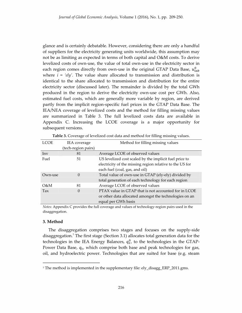
are summarized in Table 3. The full levelized costs data are available in

Appendix C. Increasing the LCOE coverage is a major opportunity for

subsequent versions.

Table 3. Coverage of levelized cost data and method for filling missing values.

LCOE IEA coverage

(tech-region pairs)

Method for filling missing values

Inv 81 Average LCOE of observed values

Fuel 51 US levelized cost scaled by the implicit fuel price to

electricity of the missing region relative to the US for

each fuel (coal, gas, and oil)

Own-use 0 Total value of own-use in GTAP (ely-ely) divided by

total generation of each technology for each region

O&M 81 Average LCOE of observed values

Tax 0 PTAX value in GTAP that is not accounted for in LCOE

or other data allocated amongst the technologies on an

equal per GWh basis

Notes: Appendix C provides the full coverage and values of technology-region pairs used in the

disaggregation.

3. Method

The disaggregation comprises two stages and focuses on the supply-side

disaggregation.5 The first stage (Section 3.1) allocates total generation data for the

technologies in the IEA Energy Balances, , to the technologies in the GTAP-

Power Data Base, , which comprise both base and peak technologies for gas,

oil, and hydroelectric power. Technologies that are suited for base (e.g. steam

5 The method is implemented in the supplementary file: ely_disagg_ERP_2011.gms.


217

turbine) and peak (e.g. combustion turbine) load provision have different cost

structures. These technological and cost differences are captured in the

disaggregation and preserved even if a modeler elects to re-aggregate the sector

into a single gas power sector. The second stage estimates new, balanced

levelized input costs that are “close” to the original data, but are consistent with

the GTAP 9 Data Base (Section 3.2). Value is allocated to the full set of GTAP

input costs based on expert assumptions and the balanced levelized input costs

found in Section 3.3. Section 3.4 discusses some basic assumptions used to create

the demand and trade dimensions of the database. The United States is used as

the example for the tables and charts in this section.

3.1 Stage 1: Base and peak load split

This particular effort is unique to many other electricity sector

disaggregations, in that the generating technologies are split into base and peak

load power. This is important for two reasons: unique cost structures of different

generating technologies and providing important insight into modeling using

the database.

First, there are many ways of converting an energy source to electricity. For

example, gas and oil can be directly combusted in a gas turbine, used to heat

water to drive a steam turbine, or some combination of these two methods (e.g.

combined cycle). Different combinations of fuels can be co-fired in the same

power plant. Moving water can be converted to electricity by damming a river,

by run-of-river, or by capturing tides. Each of these technologies have unique

cost structures due to different levels of investment and fuel efficiency. Ideally,

specific electricity generation technologies would be captured; however, these

data are not available for this version of the GTAP-Power Data Base, so base and

peak provide a coarse approximation.

Second, splitting gas, oil, and hydro into base and peak load on the supply-

side offers a first-order approximation of different technologies that are better

suited to providing base (e.g. combined cycle gas) versus peak (e.g. combustion

turbine) power. There are many ways to represent the electricity sector in CGE

modeling (e.g. Paltsev et al., 2005; Pant, 2007; Sue Wing, 2008; Château et al.,

2010; Capros et al., 2013). A modeler using this database might find it useful to

allow only technologies that are well-suited to base (or peak) to substitute. The

intent of this database is not to propose a model. Separating technologies into base

and peak in the database allow for flexibility in modeling. Of course, should the

modeler choose to pursue an alternative scheme that does not separate base and

peak power technologies, the technologies (e.g. gas base load and gas peak load)


218

could be aggregated into a single technologies (e.g. gas power)6, and the

aggregate cost structures discussed above, which includes different technologies,

would be captured. That is, the base and peak load distinction is the more

general way to disaggregate the data.

Separating the base and peak load split into a separate stage makes the

problem more tractable and allows seamless implementation of alternative data

types (e.g. detailed regional technological data) and models (e.g. Wiskich, 2014)

without compromising the matrix balancing described later in Stage 2.

The base-peak load split stage minimizes the total O&M and fuel costs of base

load production subject to GWh clearing constraints and an assumption that base

load must account for at least 85% of total GWh produced. This is a simple way

to allocate high capital, low variable cost technologies to the base load and low

capital, high variable cost technologies to peak load. A straightforward

improvement would be to minimize variable costs specifically; a portion of O&M

costs may be fixed. The following formulation is repeated for each region, r:

(1)

subject to:

(2)

(3)

(4)

(5)

where qt is the total GWh produced by each generating technology, t. Again, q0e is

total GWh produced by each energy type, e, from the IEA Energy Balance data

(the dataset does not distinguish base and peak load technologies), and l0ct is the

IEA levelized cost data for each generating technology. The set g contains all

generating technologies in the GTAP-Power Data Base (not ‘T&D’), and bl is the

subset of g with generating technologies classified as base load power. The scalar

β is the assumed proportion of base load generation in total generation. Here,

85% is assumed based on load duration curves; however, this value may change

by region. This process is shown visually in Table 4 and Table 5.

6 For example, with FlexAgg or GTAPAgg programs available on the GTAP website:

https://www.gtap.agecon.purdue.edu/.

https://www.gtap.agecon.purdue.edu/


219

Table 4. Electricity production by sectors in IEA Energy Balances for the United States,

q0e, terawatt-hours (TWh).

Nuclear Coal Gas Oil Hydro Wind Solar Other

Q0 821.4 1,872.2 1,056.6 31.4 321.7 120.9 6.2 96.3

Source: IEA Energy Balances (IEA, 2010a; IEA, 2010b).

Table 5. Generation allocated to base and peak load power for each technology based on

minimized O&M and fuel costs in the United States, qt, TWh.

Base Load (BL) Peak Load (P)

Nuclear Coal Gas Oil Hydro Wind Other Gas Oil Hydro Solar

Q 821.4 1,872.2 445.1 0 321.7 120.9 96.3 611.4 31.4 0 6.2

Source: GTAP-Power Data Base, erp.har, header: GHWR.

One important limitation in the above method is that it cannot admit more

than one technology that is both base and peak load. Alternative models which

elucidate the base and peak load split (e.g. Wiskich, 2014) could be implemented

in this stage; however, there is a trade-off between model capability, data

availability, and solution improvement.

Figure 3 shows the global shares of electricity from base and peak load

technologies. Coal, nuclear, wind, and other exclusively provide base load, and

solar exclusively provides peak load. The exclusive technologies have uniform

levelized costs; therefore, the base and peak distinction does not have any

implication on the values in the disaggregate database. Gas provides over half of

the peak load. Hydro is more likely to provide base load than peak load.

Conversely, oil is more likely to provide peak than base load.

Figure 3. Shares of global electricity generation from different technologies in base and

peak (green cut-out) load.

Source: GTAP-Power Data Base, erp.har, header: GWHR.

11.7% 41.0%

14.8%

2.0%

12.1% 1.6%

2.2%

7.6%

3.8%

3.0%

0.3%

14.7%

NuclearBL

CoalBL

GasBL

WindBL

HydroBL

OilBL

OtherBL

GasP

HydroP

OilP

SolarP


220

3.2 Stage 2a: Targeting levelized cost relationships

3.2.1 The general disaggregation problem

This section presents the matrix balancing problem and the corresponding

notation which will be used to describe the subsequent disaggregations in order

to conform to existing literature. This documentation focuses on the supply-side,

because it is the most interesting for the electricity disaggregation. The supply-

side disaggregation problem is a subset of the matrix balancing problem. The

demand and trade-side are discussed later in Section 3.4; both are based on the

resulting domestic production from the supply-side disaggregation.

The fully disaggregated supply-side matrix is constructed by disaggregating a

particular sector (e.g. electricity) into sub-sectors while the other sectors remain

unaffected. The balanced disaggregation is defined as the non-negative matrix X

with elements xit where i is an input in the same vector of inputs as those in the

full GTAP 9 Data Base, and t is a new industry within the set of new industries

(or technologies) being inserted in place of the aggregated sector. By way of

example, xit might refer to capital inputs into the solar power generation sub-

sector. In order to perform this disaggregation, we start with an initial non-

negative matrix A which is constructed from economic and/or technological

information about alternative technologies. The disaggregation problem is to

minimize the distance between the elements of X and A subject to a set of

constraints imposed by the I-O structure (Schneider and Zenios, 1990). In

particular, the sum of xit over all t (row sum) must equal the original

employment of input i in the aggregate sector defined as ui (i.e. where

).7 Most methods also impose a column sum constraint on the sum of

xit over all i for each t must equal some given value vt (i.e. where

). However, this is not required for consistency with the GTAP 9 Data

Base since the earlier row sum restriction will ensure that total value in the

disaggregate matrix will equal that of the aggregate industry. We are motivated

in this paper by the desire to avoid a potentially restrictive column sum

constraint when information on the column sum, vt, is unknown or of less

reliability than the component costs (Peters and Hertel, 2016a,b).

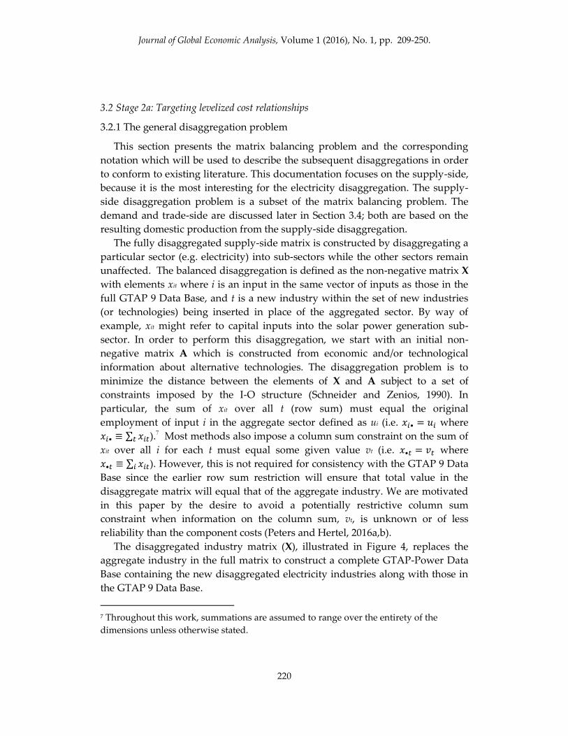
The disaggregated industry matrix (X), illustrated in Figure 4, replaces the

aggregate industry in the full matrix to construct a complete GTAP-Power Data

Base containing the new disaggregated electricity industries along with those in

the GTAP 9 Data Base.

7 Throughout this work, summations are assumed to range over the entirety of the

dimensions unless otherwise stated.


221

Technologies (t) Sum ( )

Inp

uts

(i)

Sum

( )

Figure 4. The supply-side table for the disaggregated electricity sector (X).

3.2.2. The GTAP-Power Data Base disaggregation for levelized costs

Peters and Hertel (2016b) show that an ideal disaggregation preserves both

the cost structure and “row share” (i.e. relative input cost intensity across

technologies) implied by the economic data (in this case, L0). This is especially

the case when the database will be used in a model with substitution between the

electricity generation technologies.

Other electricity disaggregations use available levelized cost data, but only

leverage one aspect of the economic relationships. Marriott (2007), Arora and Cai

(2014), and Lindner et al. (2014) focus on row shares by allocating input costs

across new technologies based largely on production (GWh) and elementary

assumptions (e.g. water transport is exclusive to coal-fired power and pipeline

transport is split between gas and oil power). In these cases, there is no specific

consideration regarding the final cost structure of the technologies. Furthermore,

these are ad hoc methods and do not present a systematic way of introducing

additional information as in constrained optimization formulations.

Sue Wing (2008) presents a positive mathematical programming approach to

incorporate cost structure and detailed engineering data (e.g. thermal efficiency,

GWh production). The formulation does quite well in introducing the detailed

technological data, but neglects specific attention to preserving input intensity

(i.e. row share) across the new technologies. Given that the input cost data exists

for the disaggregation task at hand, both relationships (i.e. cost structure and row

share) should be considered.

Outside of electricity-specific literature, maximum entropy (e.g. cross-entropy,

RAS) approaches are well-studied for matrix filling and balancing problems

considering an underdetermined and/or conflicting system (Golan et al., 1994;


222

McDougall, 1999; Robinson et al., 2001; Lenzen et al., 2009).8 However, the

disaggregation problem here is unique to the traditional cross-entropy approach

(and RAS) in two main ways: i) total column sums for each technology are

unknown and ii) the prior coefficients for the full matrix do not exist (e.g. a

previous year as suggested in Robinson et al. 2001).

The first limitation can be overcome several ways. Column sums can most

simply be derived by an allocation of value to transmission and distribution and

total levelized cost of generation (per GWh) multiplied by the total GWh of each

generating technology which is then scaled to match the total value in the

original GTAP electricity sector. This preserves relative total cost intensity across

different technologies; however, due to the inconsistent nature of the data, the

cost structures are sacrificed. Peters and Hertel (2016b) show that this is

problematic in the case of substitution between generating technologies, and

results can be greatly improved by eliminating the overly-restrictive column

constraint which is derived from disparate data sources.

Instead, the fully disaggregated matrix is partitioned to investment, fuel,

O&M, own-use, and production tax costs for transmission and distribution and

each generating technology. This provides a target matrix, A, based on the

levelized cost and electricity production data; however, it is inconsistent with the

GTAP Data Base. Targeting relationships in levelized cost data, L0, and fixing the

other data implies that the GTAP values, U0, as an aggregate measure, and the

electricity production values, Q, are the more trusted sources.9 The proposed

optimization algorithm finds an estimated levelized cost which minimizes

deviation from both the derived i) cost proportionality within a single generating

technology (i.e. cost structure) and ii) relative cost intensity between generating

technologies (i.e. row share) from the target levelized cost data. In doing so, the

algorithm targets relationships between levelized costs rather than the levelized

8 There are also minimized sum-squared error-type and other approaches; however,

GTAP is constructed using cross-entropy methods, so a cross-entropy approach is used

for the GTAP-Power Data Base. 9 It must be noted that traditional levelized cost has previously been shown to be a

flawed metric as it treats electricity as a strictly homogenous product with a value that

does not change in terms of space (e.g. availability of renewable use), time (e.g. base and

peak demand periods, seasonal variability, intermittency of some renewables), or lead-

time (Joskow, 2011; Hirth et al., 2014). Furthermore, there is uncertainty in the parameters

(e.g. discount rate, efficiency, heat rate, load factor, lifetime) used to derive the costs. In

light of this particular problem, levelized costs are still insightful despite their obvious

limitations.


223

costs themselves. Tax costs are assumed fixed and are assigned by the value

implied by the tax (L0) and production (Q) data. The residual tax value in GTAP

are allocated to the new sectors on a per GWh basis.

The objective function is designed to minimize weighted entropy distance

from both the cost structure and row share relationships (Peters and Hertel,

2016a).10 This is termed the share-preserving cross-entropy (SPCE) method.

Constraints are imposed to maintain an assumed allocation of value to

transmission and distribution and ensure consistency with the GTAP Data Base.

The target matrix A, as defined in Section 3.2.1, is given by:

(6)

where

or the total value of the GTAP electricity sector. The

balanced matrix X, as defined in Section, 3.2.1, is given by:

(7)

where lct are the balanced levelized costs after balancing with the SPCE method.

The set of linear constraints are described as:

(8)

Again, the index r is dropped for simplicity since each are performed

independently from one another. The balanced levelized costs lct are determined

from the SPCE objective and constraints as follows and repeated for each region,

r:

(9)

subject to:

(10)

10 A variant of Kuroda (1988) is a sum squared error-type matrix balancing method that is

also capable of removing the total cost constraint. We employ the SPCE because the

GTAP Data Base is also created with an entropy approach.


224

(11)

The SPCE method is written in terms of X and A to conform to literature and

for sake of simplicity, but are written in terms of lct and qt in the accompanying

GAMS code. The final matrix of L is the estimated levelized cost which

minimizes the weighted entropy distance from the economic relationships

implied by the target levelized cost data (L0). The first natural-log component of

the objective targets cost structure, and the second targets row share. The set c

consists of all the levelized costs, and subset d are the levelized costs excluding

effective tax. The objective, Equation 9, sums across only d since the effective tax

is fixed (discussed in Section 4.3.5).

The first constraint (Equation 10) sums over only the costs, i, which are

associated with the particular levelized cost, c (e.g. labor in O&M, coal in fuel; see

Table 2). The vector U0 is the GTAP national input value data for total value of

each cost in the original electricity sector (‘ely’) with dimensions for source (a)

and type (b). This ensures market clearance of the GTAP values across each

levelized costs; that is, values of the new sectors in the GTAP-Power Data Base

can be aggregated to the GTAP 9 Data Base electricity values.

The second constraint (Equation 11) ensures the assumed value allocation to

transmission and distribution where the scalar γ is the proportion of total non-

tax value allocated to the transmission and distribution sector. The γ value does

not have a great deal of literature behind it; examples of values include 4%

(Marriott, 2007), 45% (Joskow, 1997), and 65% (Sue Wing, 2008) for the United

States. The non-production operational expenses (i.e. transmission, distribution,

customer accounts, customer service, sales, and administration) for electric

utilities in the United States represent about 21% of total operational expenses

(EIA, 2013: Table 8.3).11 Therefore, a γ value of 21% is used for all regions in this

disaggregation. In reality, the value may differ regionally which can easily be

incorporated provided accurate data are available.

Additional constraints are imposed to ensure sufficient and proportional

allocation of fuels into their associated technologies (e.g. total fuel costs of coal-

based generation are greater or equal to the total coal costs to electricity in the

GTAP Data Base).

11 This does not include electricity loss in transmission and distribution. Here, we are

concerned with the costs and values.


225

3.3 Stage 2b: Targeting specific input costs for the levelized cost

Stage 2a returns estimated total column sums for each levelized cost (Table 6)

which overcomes the unknown total costs which motivated the SPCE

formulation. Therefore, RAS can be used to estimate the matrices for each

levelized cost. Basic data and assumptions are used to construct the target

matrices (the same A as defined in Section 3.2.1) for each levelized cost

separately. The notation is identical to the generic disaggregation problem in

3.2.1 and pertains to the relevant section only. That is, A is not differentiated by

any form of notation in the O&M and capital disaggregations in the following

sections. They are independent disaggregations.

Table 6. Values for the United States implied by the levelized cost and production data

for each technology subject to market clearing in the GTAP values (uc).

Base Load (BL) Peak Load (P)

c TnD Nuc. Coal Gas Wind Hydro Oil Other Gas Hydro Oil Solar uc

Inv 24.8 22.5 36.9 4.1 7.3 28.7 0.0 2.3 3.6 0.0 0.4 1.2 130.0

Fuel 0.0 0.0 37.9 22.6 0.0 0.0 0.0 3.1 42.0 0.0 6.7 0.0 117.9

Own-

use 5.5 3.9 8.9 2.1 0.6 1.5 0.0 0.5 2.9 0.0 0.1 0.0 26.0

O&M 43.7 18.8 16.5 1.7 2.0 4.3 0.0 1.9 2.8 0.0 0.7 0.1 133.1

Tax 5.2 -4.8 8.5 2.0 -0.1 0.5 0.0 0.1 2.8 0.0 0.1 0.0 14.4

Source: GTAP-Power Data Base, erp.har, headers: ZLCO and ELYT.

3.3.1 Operating and maintenance costs

There is little information regarding the specific sectoral composition of

the O&M levelized cost matrix. The GTAP 9 Data Base has 56 costs which fall

broadly under the umbrella of O&M costs including five labor classes and

various agricultural, machinery, chemical, and transportation sectors (see

Appendix A for the full mapping). While not much data exists regarding how

these sub-sectors enter either transmission and distribution or specific generating

technologies, some basic assumptions can be made regarding their shares. These

shares can be treated as probabilities that an input cost enters the new sectors.

This is similar to a technique previously employed to allocate capital between

transmission and distribution and generation (Sue Wing, 2008) and to allocate

costs to different generation types for input-output analysis (Marriott, 2007).

These basic assumptions are be formulated into two tables. The first table

allocates the assumed shares of a particular sub-sector entering transmission and

distribution versus generation as a whole, Pt (treated akin to probabilities with

costs as uncertain). The second table allocates assumed probabilities between the

various generating types conditional on the cost entering generation (Pg). Targets


226

are constructed from these probabilities. The assumptions for Pt and Pg used in

this work are presented in Appendix B.

Table 7. Probability tables for allocation between transmission and distribution (Pt) and

allocation of conditional probabilities between generation types (Pg).

Pt Pg

TnD GEN Total Nuclear … Solar Total

O&M 1 1 O&M 1 1

… 1 … 1

O&M n 1 O&M n 1

Probabilities between transmission and distribution and generation are also

based on the cost proportion allocated to transmission by the earlier transmission

and distribution share assumption, γ. The resulting probabilities are:

(12)

(13)

where PtT&D is the probability of cost classified as transmission and distribution,

and PtGEN is the probability of cost classified as generation (PtGEN = 1- PtT&D).

Likewise, there is also a probability of the input cost entering the specific

generation technologies allocated based on relative levelized O&M costs across

technologies (i.e. row share for O&M in Table 6), termed Prg.

(14)

where g is the set of generating technologies only. Alternatively, Prg could be

derived based on other assumptions (e.g. construction costs mimic levelized cost

of capital rather than O&M). Such decisions are dependent on the researcher and

problem, but the framework presented here is flexible to such convictions. Since

Pg and Pr are independent, the total probability of the O&M cost for a generating

technology conditional on entering generation is therefore the intersection of Pg

and Pr:

(15)

The resulting tax-inclusive targets, AI, for each O&M cost can be written as:

(16)


227

(17)

where aIi,t is the tax-inclusive (I) target for input costs, i, to new industries, t,

where i here refers to the subset of 56 costs in the GTAP Data Base which are

classified as O&M costs (i.e. ). Table 8 shows a visual representation of

the targeting matrix.

Table 8. Target the individual components of O&M costs.

Target O&M cost sub-matrix (AI)

Base load Peak

TnD Nuc Coal Gas Oil Hydro Wind Other Gas Oil Hydro Solar

O&M 1

…

O&M n

Total

Notes: A similar procedure is used for capital, fuel and tax sub-matrices.

The RAS method is formulated as follows:

(18)

subject to:

(19)

(20)

where xIit is the estimated tax-inclusive value of O&M costs. The first constraint

(Equation 19) pertains to the market clearance conditions, and the second

(Equation 20) pertains to the column sum estimated in Stage 2a. This procedure

is repeated for each region. The tax-inclusive estimated cost (xI) is expanded to

full GTAP dimensionality based on the source and type proportions of the

original GTAP electricity sector proportions which ensures market clearing in the

additional dimensions. The results for the United States are discussed in Section

4.3.

3.3.2 Fuel costs

There are five sectors in the GTAP Data Base which correspond to fuel costs:

coal, gas pipeline, distributed gas, oil, and petroleum and coal products (‘coa’,

‘gas’, ‘gdt’, ‘oil’, and ‘p_c’ in GTAP, respectively). These are allocated using basic

assumptions and conditionals when those assumptions break down. The original


228

GTAP coal sector is allocated to ‘CoalBL’. Both pipeline and distributed gas are

allocated to ‘GasBL’ and ‘GasP’ based on the relative levelized cost between the

technologies and in a manner where the proportion of types of gas are equal for

each technology. The equal proportions technique is also used for oil and ‘p_c’ in

‘OilBL’ and ‘OilP’; however, petroleum-derived products do not strictly enter oil

technologies (e.g. lubricants, gasoline for company vehicles). The excess ‘p_c’ is

used to meet the levelized fuel cost column sum constraints for the other sectors.

Conditionals may come into play where there are fuel inputs to electricity in

the original GTAP Data Base, but there is no directly corresponding generation

for a region (e.g. coal input to electricity in GTAP, but no coal generation in the

OECD GWh data). The source of these residuals is case and region-specific, but

may arise as a result of sectoral aggregation in GTAP, non-exclusivity of fuel use

for electricity production (e.g. gas for heat in the facility), and the balancing

algorithm necessary for the original GTAP Data Base. In these cases, targets are

created based on relative cost across the new sectors. High confidence in the

assumptions for fuel inputs to generating technologies results in a highly

constrained optimization problem.

3.3.3 Capital costs

Although levelized investment costs only have one associated GTAP sector

(i.e. ‘Capital’), the difference in type (i.e. basic and tax) costs are of particular

importance in the electricity sector. For instance, the United States has

investment tax credits which subsidizes capital investments to some renewable

technologies. This is an important consideration for modeling using the

disaggregated database. The targets for the two type matrices are as follows:

(21)

(22)

where aIit is the tax-inclusive target (superscript I), and aXit is the tax-exclusive

target (superscript X) for investment costs. The set i is a subset of all costs which

pertain to investment costs ( , which is only ‘Capital’ in this case). The

scalar k0it is the power of the tax on capital for the electricity sub-sectors.

Entropy is minimized for a tax-inclusive and tax-exclusive matrix subject to

market clearing constraints for both matrices and a total column sum for the tax-

inclusive matrix. This is a similar formulation to one found in McDougall (1999).


229

(23)

subject to:

(24)

(25)

(26)

The results, xX and (xI – xX), the basic and tax matrices, are expanded to full

GTAP dimensionality based on the source in the original GTAP electricity sector

proportions to preserve market clearing in these dimensions.

3.3.4 Own-use costs

The value of total own-use in the electricity sector in each region comes

directly from own-use in the original GTAP Data Base, where i = ely. The

total costs of own-use for the disaggregated electricity sectors is the estimated

levelized cost for own-use, lown-use,t, multiplied by the total production, qt.

The individual electricity input costs are allocated to the new electricity

sectors with the assumption that each demands identical shares of transmission

and distribution and generating technologies. This is as though they draw from

the grid and not necessarily the individual plant-type.

3.3.5 Effective production tax

The effective production tax in GTAP is labeled ‘PTAX’, which for a

generating technology can be thought of a tax on a specific type of generation,

while ‘PTAX’ for transmission and distribution can be thought of a tax on

electricity provision to the ultimate users. Tax costs are assumed fixed and are

assigned by the value implied by the levelized tax from the data (L0) and total

GWh production (Q) data. The residual tax value (that not explained by available

tax data) is additionally allocated to the new sectors on an equal per GWh basis.

3.4 Demand-side and trade disaggregation

The electricity mix of exports of electricity are assumed to be identical to the

mix of domestic production. This assumption fills the complete trade matrix.

The demand-side share allocation for each electricity sector is simply identical to

the mix implied by the sum of domestic production and the net imports.


230

Presumably, different industries and households consume electricity from

different sources depending on the sub-region and type of load. For instance, the

retail industry may consume electricity predominantly during peak hours during

the middle of the day. Households may consume more electricity during the

peak hours immediately following school or office hours. Furthermore,

households may demand renewable sources or even purchase household solar

panels. Certain industries may require electricity and make long-term

agreements for base load electricity.

Unfortunately, anything beyond pure assumption is currently unavailable for

this research. The disaggregation of the demand-side in the GTAP-Power Data

Base assumes all users demand identical shares of transmission and distribution

and each generating technologies.

Alternatively, the transmission and distribution sector could be separated

from generation where generation would be sold to transmission and

distribution, and users would purchase the transmission and distribution. This

may make some sense in terms of how the electricity sector operates (at least in

the United States); however, this type of database construction does not allow for

different generation demands by industry. The database construction described

above is general enough to allow for this; although due to data limitations,

uniform mixes across industries are assumed for this particular version.

4. Results

The final results of the supply-side disaggregation are presented in this

section. The demand-side is less interesting because of the lack of available data.

The data and assumptions explained above are available upon request. This

section focuses on the error between the estimated levelized costs and the

IEA/NEA data and how important features in the original datasets are captured

in the disaggregated data.

4.1 Ad hoc Method for Large Deviations

For some regions the deviation between the estimated and the target levelized

costs can be quite large. While deviation is expected, large deviations may

indicate broader issues in the OECD electricity production and, more likely, the

electricity sector in the GTAP Data Base. For instance, the target estimate of

capital requirements for electricity in Cambodia derived from the levelized costs

and production data is 75.9 million USD; however, the GTAP Data Base reports

only 1.8 million USD of capital is allocated to the entire electricity sector.


231

Obviously, there is some discrepancy in reporting between the top-down and

bottom-up type datasets.

To accommodate for largely disparate data, an additional bound constraint is

added to the Stage 2a formulation which bounded the estimated capital and

O&M levelized costs for each generation technology to n and (1/n) times the

target levelized cost value threshold. Fuel cost are excluded from these bounds

because these are generally directly mapped to fuel input costs in GTAP (e.g.

coal to ‘CoalBL’) and the costs are highly variable across regions which limits the

relevance of using an average of available levelized cost data as an initial

estimate. A single capital and O&M levelized cost to a generation technology

which deviates by n or (1/n) times the target estimate results in an unsuccessful

completion. The number of successful completions in total share of GWh terms

are shown in Figure 5. Beyond a certain threshold (x-axis) it may be better to

allocate each levelized cost using an ad hoc method. The threshold chosen is 10

because at this point over 95% of the global GWh produced converges using the

SPCE method.12

Figure 5. Share of total GWh which converge using the SPCE procedure with the bound

of deviation from target LCOE data.

Source: GTAP-Power Data Base, erp.har, header: OPTS.

12 With a threshold of a 10 or 1/10 times deviation from the original levelized cost value

the following 22 regions cannot be reconciled: Oman, Rest of Oceania, Brunei

Darussalam, Laos, Rest of South Asia, Argentina, Ecuador, Honduras, Estonia, Lithuania,

Belarus, Rest of Former Soviet Union, Georgia, Bahrain, United Arab Emirates, Rest of

West Asia, Guinea, Rest of West Africa, Kenya, Madagascar, Malawi, and Rest of

Southern Africa. These regions produce less than 3% of the world’s electricity and in

most cases would be aggregated into larger regions.

0%

20%

40%

60%

80%

100%

1 2 3 4 5 6 7 8 9 10 11 12 13 14 15 16 17 18 19 20

Sh

are

of

tota

l G

Wh

Multiplicative bound on deviation from target levelized cost


232

The ad hoc method is used for those regions that do not converge and follows

Marriott (2007), Lindner et al. (2014), and Arora and Cai (2014) by allocating each

costs by the production weighted levelized costs described by for each

unsuccessful region:

(27)

This does not specifically preserve the cost structure, but the data is so

disparate in these regions the any modeling of these regions individually is

suspect to begin with.

The jump in GWh converging from a bound of 9 to 10 in Figure 5 is due to

the convergence of Russia at a bound of 10. The GTAP value of capital in Russia

is much lower than the value implied by the target levelized cost of capital.

Section 6 discusses how the GTAP Data Base construction may be able to

leverage the levelized cost data to eliminate such large discrepancies moving

forward while recognizing the limitations in the target cost data as well.

4.2 Deviation from target levelized cost data

It is worth reiterating that the procedure described above implies that the

GTAP values, as an aggregate measure, and the electricity production values are

a more trustworthy source than levelized cost, as a stylized representative of

actual costs determined from a number of assumptions. This is why we fix the

GTAP, U0, and the estimated GWh production, Q, values and target the levelized

costs, L0.

Table 9 shows the percentage deviation of the estimated levelized costs from

the target levelized costs in the United States. The average deviation for non-

fixed levelized costs is 20.9%. The estimated levelized cost for ‘NuclearBL’ and

‘CoalBL’ are larger than the target levelized cost while the majority of others are

lower. It is also evident that the O&M cost in the GTAP data is much larger than

the cost implied by O&M in the levelized cost; the deviation is highest for O&M

costs and the balanced estimates are all larger than the target levelized costs. The

frequency plot in Figure 6 shows how these deviations are distributed for all

regions, and Figure 7 shows the different between OECD and non-OECD

countries.

Table 10 and Table 11 show the deviation from the cost structure and relative

cost intensity for the United States, respectively. Again, the disparity between the

target levelized costs and the GTAP data in O&M is the primary source of

deviation in cost structure. However, the relative fuel costs seem to be the

primary source of deviation in the row share. The effective tax has no deviation


233

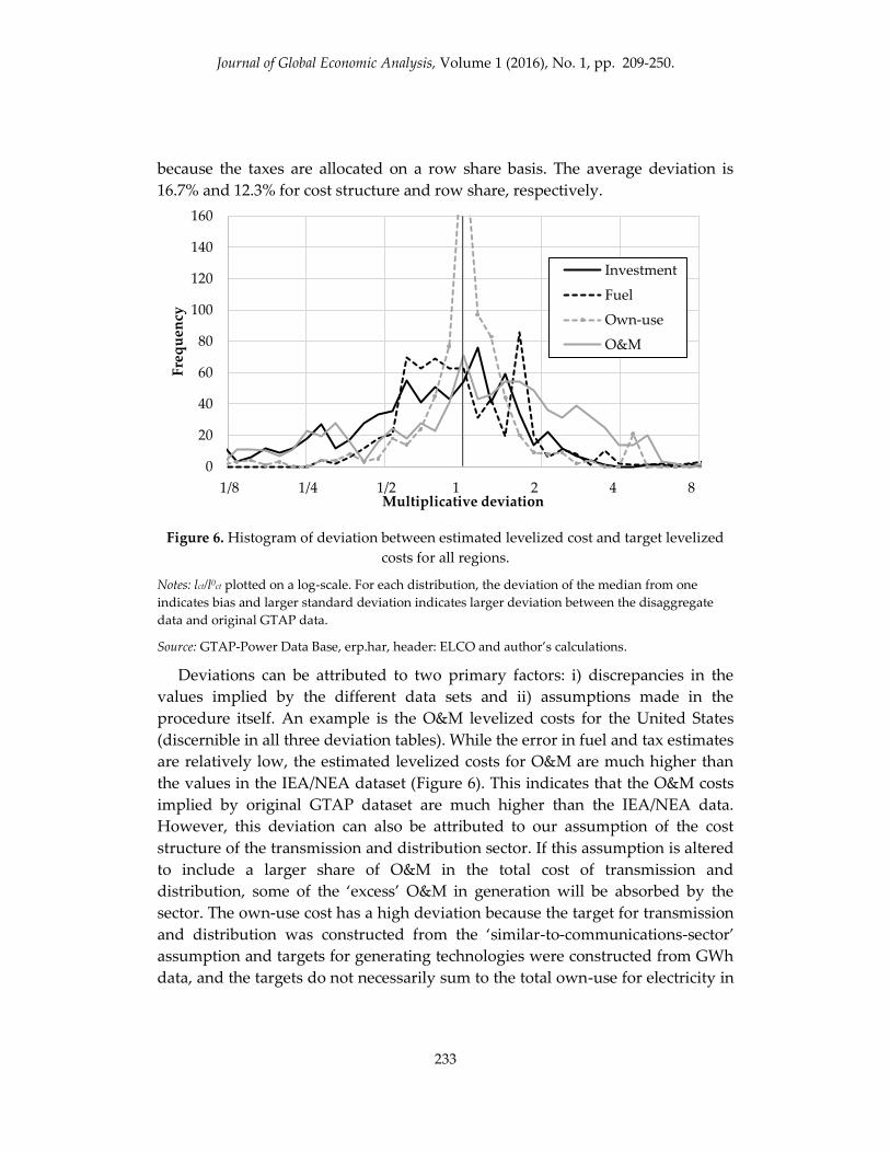
because the taxes are allocated on a row share basis. The average deviation is

16.7% and 12.3% for cost structure and row share, respectively.

Figure 6. Histogram of deviation between estimated levelized cost and target levelized

costs for all regions.

Notes: lct/l0ct plotted on a log-scale. For each distribution, the deviation of the median from one

indicates bias and larger standard deviation indicates larger deviation between the disaggregate

data and original GTAP data.

Source: GTAP-Power Data Base, erp.har, header: ELCO and author’s calculations.

Deviations can be attributed to two primary factors: i) discrepancies in the

values implied by the different data sets and ii) assumptions made in the

procedure itself. An example is the O&M levelized costs for the United States

(discernible in all three deviation tables). While the error in fuel and tax estimates

are relatively low, the estimated levelized costs for O&M are much higher than

the values in the IEA/NEA dataset (Figure 6). This indicates that the O&M costs

implied by original GTAP dataset are much higher than the IEA/NEA data.

However, this deviation can also be attributed to our assumption of the cost

structure of the transmission and distribution sector. If this assumption is altered

to include a larger share of O&M in the total cost of transmission and

distribution, some of the ‘excess’ O&M in generation will be absorbed by the

sector. The own-use cost has a high deviation because the target for transmission

and distribution was constructed from the ‘similar-to-communications-sector’

assumption and targets for generating technologies were constructed from GWh

data, and the targets do not necessarily sum to the total own-use for electricity in

0

20

40

60

80

100

120

140

160

1/8 1/4 1/2 1 2 4 8

Fre

qu

ency

Multiplicative deviation

Investment

Fuel

Own-use

O&M


234

the GTAP data. While the error values for the United States and some other

OECD countries are relatively low, the errors can be quite high for regions where

the GTAP and IEA electricity production data are questionable and where the

levelized cost is derived through averages.

Figure 6 shows that O&M costs are skewed to the right which indicates that

GTAP, in general, has more O&M cost than the levelized cost data. However, at

the left-hand extremum for both investment and O&M costs, Figure 6 shows that

for some regions and technologies there is significantly less value in the GTAP

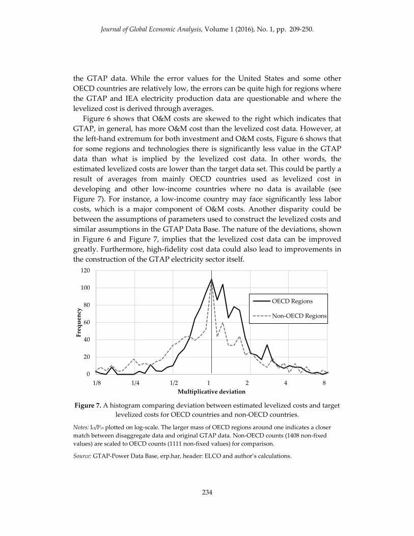
data than what is implied by the levelized cost data. In other words, the

estimated levelized costs are lower than the target data set. This could be partly a

result of averages from mainly OECD countries used as levelized cost in

developing and other low-income countries where no data is available (see

Figure 7). For instance, a low-income country may face significantly less labor

costs, which is a major component of O&M costs. Another disparity could be

between the assumptions of parameters used to construct the levelized costs and

similar assumptions in the GTAP Data Base. The nature of the deviations, shown

in Figure 6 and Figure 7, implies that the levelized cost data can be improved

greatly. Furthermore, high-fidelity cost data could also lead to improvements in

the construction of the GTAP electricity sector itself.

Figure 7. A histogram comparing deviation between estimated levelized costs and target

levelized costs for OECD countries and non-OECD countries.

Notes: lct/l0ct plotted on log-scale. The larger mass of OECD regions around one indicates a closer

match between disaggregate data and original GTAP data. Non-OECD counts (1408 non-fixed

values) are scaled to OECD counts (1111 non-fixed values) for comparison.

Source: GTAP-Power Data Base, erp.har, header: ELCO and author’s calculations.

0

20

40

60

80

100

120

1/8 1/4 1/2 1 2 4 8

Fre

qu

ency

Multiplicative deviation

OECD Regions

Non-OECD Regions


235

Table 9. Percent deviation from non-fixed target levelized cost for each generating technology for the United States.

Levelized cost T&D NuclearBL CoalBL GasBL WindBL HydroBL OtherBL GasP OilP SolarP

Investment -10.5% 5.0% 10.0% -16.9% -4.1% -7.5% -5.4% -17.2% -16.1% -9.6%

Fuel -19.2% - 63.0% -25.1% - - -14.6% -25.1% -24.2% -

Own-use -8.7% 7.0% 12.0% -15.2% -2.1% -5.6% -3.5% -15.5% -14.4% -7.7%

O&M 34.0% 57.0% 64.0% 24.0% 43.0% 38.0% 41.0% 41.0% 24.0% 35.0%

Effective tax - - - - - - - - - -

Note: The average absolute deviation for non-fixed values is 21.3%.

Source: GTAP-Power Data Base, erp.har, header: ELCO.

Table 10. Percent deviation from non-fixed target shares of levelized cost in the total cost (i.e. cost structure) of each specific

generating technology in the United States.


Investment -21.9% -19.1% -19.2% 3.0% -9.3% -5.9% -7.9% 4.0% 3.0% -3.6%

Fuel -29.5% - 20.0% -7.1% - - -16.8% -6.1% -6.6% -

Own-use -20.3% -17.5% -17.5% 5.0% -7.4% -3.9% -6.0% 6.0% 6.0% -1.7%

O&M 17.0% 21.0% 21.0% 54.0% 35.0% 40.0% 37.0% 37.0% 55.0% 44.0%

Effective tax -12.7% -23.1% -26.6% 24.0% -5.4% 2.0% -2.6% 2.6% 25.0% 7.0%


Source: GTAP-Power Data Base, erp.har, header: EL10.

Table 11. Percent deviation from non-fixed target relative cost intensity (i.e. row share) normalized by GWh for each levelized

cost and generating technology in the United States.


Investment -9.3% 7.0% 12.0% -15.7% -2.8% -6.2% -4.1% -16.1% -15.0% -8.3%

Fuel -23.0% - 55.0% -28.7% - - -18.6% -28.7% -27.8% -

Own-use -8.7% 7.0% 12.0% -15.2% -2.1% -5.6% -3.5% -15.5% -14.4% -7.7%

O&M -7.2% 9.0% 14.0% -13.7% -0.5% -4.0% -1.9% -1.9% -14.1% -6.2%

Effective tax - - - - - - - - - -


Source: GTAP-Power Data Base, erp.har, header: ELC9.


236

4.3 Main result

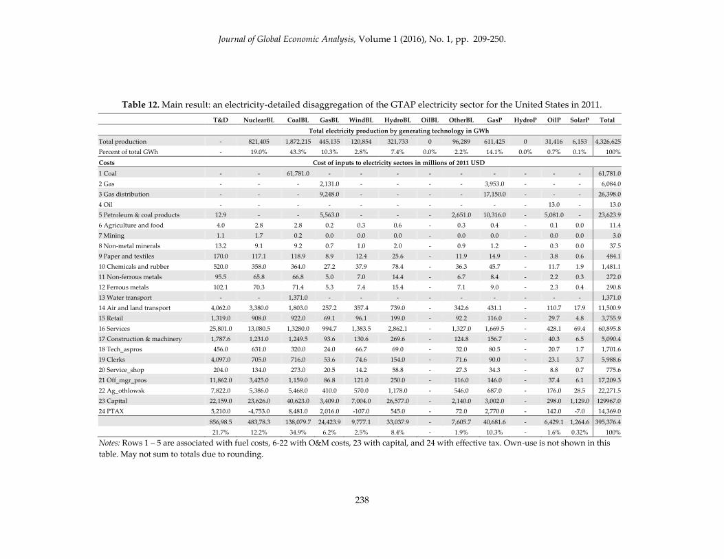
Table 12 shows the input values to the disaggregated sectors for the United

States. All of the original 62 costs were disaggregated using the method

described above, and the results are then aggregated to 21 sectors for analysis

(See Appendix A for sectoral mapping). The values are the sum of sources and

type dimensions. With the exception of a capital subsidies to solar power

(‘SolarP’) and balancing of the capital across the other users, the hidden

dimensions are allocated in identical proportions.

The fuel sectors (i.e. coal, gas, gas distribution, oil, and petroleum products)

are allocated to the corresponding generating technology. Coal enters ‘CoalBL’,

Oil enters ‘OilP’ only as there is no GWh generated from oil technology as base

load in the United States. Gas extraction and gas distribution enter in equal

proportion to ‘GasBL’ and ‘GasP’. However, the proportion of gas fuels in ‘GasP’

to gas fuels in ‘GasBL’ is greater than the proportion of GWh in ‘GasP’ to ‘GasBL’

due to a higher levelized cost of fuel for peak gas production (i.e. less efficient

production from peak-type technologies). The opposite is true when looking at

capital to the gas generating technologies because ‘GasBL’ is more capital

intensive than ‘GasP’. A portion of petroleum products also enter ‘GasBL’ and

‘GasP’ in order to reach the levelized cost target (i.e. the total gas inputs in GTAP

were insufficient). The petroleum and coal products sector in GTAP contains

many different energy fuels (e.g. coke, refinery gas, diesel), so it is difficult to

distinguish the actual composition of this sector. As discussed previously, some

of these energy fuels may very well enter alternative types of production other

than strictly oil technologies. These also enter in fixed proportion between gas

technologies. Similarly, the relative levelized cost intensities between

technologies is preserved when we look at the other levelized costs and

generating technologies as well.

Recall from Section 3.3.1 that targets for each O&M cost are based on the

balanced levelized input intensity, Pr, and expert assumptions of the probability

of a cost entering T&D versus generation, Pt, and entering a specific technology,

Pg. The probability tables, Pt and Pg, used in the disaggregation can be found in

Appendix B. Focusing on two O&M sectors which had no additional

assumptions beyond relative cost intensity between technologies, chemicals &

rubber and non-ferrous metals, we see that the relative costs are similar across

the technologies. The ratio of value of chemicals and rubber to non-ferrous

metals is approximately 10.7 for each technology.

However, general assumptions can be made about many O&M sectors. First,

water transport is allocated strictly to ‘CoalBL’ (i.e. Pt(GEN) = 1 and Pg(CoalBL) =


237

1), since coal is generally the only fuel source which is transported domestically

by waterway in the United States. Second, a 2/3 probability of Pt(T&D) was made

for various sectors in the services set under the assumption that a majority of the

sales, customer service, etc. of the utilizes fall under these sectors in transmission

and distribution. This is a simple and somewhat arbitrary value, but

demonstrates the ability to add expert intuition into the methodology. A similar

method can be adopted to redistribute skilled and unskilled labor. This may

require a balancing act between relative probabilities between types of labor

within a technology and across technologies. The complex allocations of these

two labor types in generation demonstrate how some of these assumptions may

sacrifice transparency of the final results. These results show that the skilled to

unskilled labor ratio is higher for ‘NuclearBL’ and renewable sources (i.e.

‘WindBL’ and ‘SolarP’) than fossil-fuel based generating technologies.

Table 12 shows the results for the United States. It is worth noting that the

technological structure of the power sector differs greatly between countries

(shown in Figure 8). Non-fuel-based technologies would be implicitly captures in

the original GTAP Data Base as capital inputs to electricity. These technologies

comprise a large share electricity production in many large economies (e.g.

Brazil, Korea, Russia, Germany, US). The GTAP-Power Data Base captures the

technological composition of the power sector to support CGE modeling of

technology-specific policies.

Figure 8. The structure of the electric power for several large economies.

Source: GTAP-Power Data Base, erp.har, header: GWHR.

0%

10%

20%

30%

40%

50%

60%

70%

80%

90%

100% OilP

OilBL

GasP

GasBL

CoalBL

SolarP

HydroP

OtherBL

HydroBL

WindBL

NuclearBL


238

Table 12. Main result: an electricity-detailed disaggregation of the GTAP electricity sector for the United States in 2011.

T&D NuclearBL CoalBL GasBL WindBL HydroBL OilBL OtherBL GasP HydroP OilP SolarP Total

Total electricity production by generating technology in GWh

Total production - 821,405 1,872,215 445,135 120,854 321,733 0 96,289 611,425 0 31,416 6,153 4,326,625

Percent of total GWh - 19.0% 43.3% 10.3% 2.8% 7.4% 0.0% 2.2% 14.1% 0.0% 0.7% 0.1% 100%

Costs Cost of inputs to electricity sectors in millions of 2011 USD

1 Coal - - 61,781.0 - - - - - - - - - 61,781.0

2 Gas - - - 2,131.0 - - - - 3,953.0 - - - 6,084.0

3 Gas distribution - - - 9,248.0 - - - - 17,150.0 - - - 26,398.0

4 Oil - - - - - - - - - - 13.0 - 13.0

5 Petroleum & coal products 12.9 - - 5,563.0 - - - 2,651.0 10,316.0 - 5,081.0 - 23,623.9

6 Agriculture and food 4.0 2.8 2.8 0.2 0.3 0.6 - 0.3 0.4 - 0.1 0.0 11.4

7 Mining 1.1 1.7 0.2 0.0 0.0 0.0 - 0.0 0.0 - 0.0 0.0 3.0

8 Non-metal minerals 13.2 9.1 9.2 0.7 1.0 2.0 - 0.9 1.2 - 0.3 0.0 37.5

9 Paper and textiles 170.0 117.1 118.9 8.9 12.4 25.6 - 11.9 14.9 - 3.8 0.6 484.1

10 Chemicals and rubber 520.0 358.0 364.0 27.2 37.9 78.4 - 36.3 45.7 - 11.7 1.9 1,481.1

11 Non-ferrous metals 95.5 65.8 66.8 5.0 7.0 14.4 - 6.7 8.4 - 2.2 0.3 272.0

12 Ferrous metals 102.1 70.3 71.4 5.3 7.4 15.4 - 7.1 9.0 - 2.3 0.4 290.8

13 Water transport - - 1,371.0 - - - - - - - - - 1,371.0

14 Air and land transport 4,062.0 3,380.0 1,803.0 257.2 357.4 739.0 - 342.6 431.1 - 110.7 17.9 11,500.9

15 Retail 1,319.0 908.0 922.0 69.1 96.1 199.0 - 92.2 116.0 - 29.7 4.8 3,755.9

16 Services 25,801.0 13,080.5 1,3280.0 994.7 1,383.5 2,862.1 - 1,327.0 1,669.5 - 428.1 69.4 60,895.8

17 Construction & machinery 1,787.6 1,231.0 1,249.5 93.6 130.6 269.6 - 124.8 156.7 - 40.3 6.5 5,090.4

18 Tech_aspros 456.0 631.0 320.0 24.0 66.7 69.0 - 32.0 80.5 - 20.7 1.7 1,701.6

19 Clerks 4,097.0 705.0 716.0 53.6 74.6 154.0 - 71.6 90.0 - 23.1 3.7 5,988.6

20 Service_shop 204.0 134.0 273.0 20.5 14.2 58.8 - 27.3 34.3 - 8.8 0.7 775.6

21 Off_mgr_pros 11,862.0 3,425.0 1,159.0 86.8 121.0 250.0 - 116.0 146.0 - 37.4 6.1 17,209.3

22 Ag_othlowsk 7,822.0 5,386.0 5,468.0 410.0 570.0 1,178.0 - 546.0 687.0 - 176.0 28.5 22,271.5

23 Capital 22,159.0 23,626.0 40,623.0 3,409.0 7,004.0 26,577.0 - 2,140.0 3,002.0 - 298.0 1,129.0 129967.0

24 PTAX 5,210.0 -4,753.0 8,481.0 2,016.0 -107.0 545.0 - 72.0 2,770.0 - 142.0 -7.0 14,369.0

856,98.5 483,78.3 138,079.7 24,423.9 9,777.1 33,037.9 - 7,605.7 40,681.6 - 6,429.1 1,264.6 395,376.4

21.7% 12.2% 34.9% 6.2% 2.5% 8.4% - 1.9% 10.3% - 1.6% 0.32% 100%

Notes: Rows 1 – 5 are associated with fuel costs, 6-22 with O&M costs, 23 with capital, and 24 with effective tax. Own-use is not shown in this

table. May not sum to totals due to rounding.


239

5. Looking back at the GTAP Data Base construction

There may exist some opportunity to reconcile the aggregate electricity value

implied by the disaggregated levelized cost data with those from original

aggregate GTAP electricity sector. Table 13 below shows the aggregate value of

inputs to the electricity sector in the US implied by the disaggregated data

compared to those in the GTAP Data Base with an aggregate electricity sector.

The latter is a constraint on disaggregation, so it is also identical to the aggregate

electricity sector in the GTAP-Power Data Base. This section presents ideas, as

opposed to guidelines, on how such a reconciliation might be performed in

subsequent versions.

Table 13. Deviation between total aggregate inputs to the electricity sector implied by the

disaggregate data (used as targets) and the original values in the GTAP 9 Data Base ‘ely’

sector (used as consistency constraints) for the United States.

Total aggregate inputs to electricity (millions of 2011 USD)

c Aggregate value implied by

disaggregate data (Q, L0)

GTAP ‘ely’ sector

(uc)

Deviation

Inv 131,763 129,967 1.4%

Fuel 112,309 117,899 -4.7%

Own-

use 26,002 26,002 0.0%

O&M 92,575 133,139 -30.5%

Tax 14,370 14,370 0.0%

Total 377,020 421,378 -10.5%

Source: GTAP-Power Data Base, erp.har, headers: ZLCO and ELYT.

On one hand there is the “bottom-up” data constructed from levelized costs

and production levels. Recall that due to the heterogeneous reality of electricity

markets these levelized costs can be misleading in many ways (Joskow, 2011;

Hirth et al. 2014). On the other hand the aggregate GTAP electricity sector is

constructed from targets that are derived from various sources, namely

contributed I-O tables and IEA energy data. Even in the long-run, it is unlikely

that the I-O tables contributed by the GTAP community will include all or even

some of the electricity sub-sectors described here. Many contributions may not

even include a separated electricity sector. Therefore, the new electricity sectors

described here will likely remain a disaggregation of an aggregate electricity

sector in the main GTAP Data Base construction.

Therefore, despite the known limitations, there may be opportunity to use the

levelized cost data to create targets for the aggregate electricity sector in GTAP,


240

especially where quality data may not exist to target the sector otherwise. This

would help reconcile the “bottom-up” and “top-down” perspectives of the

electricity sector.

There are at least three distinct cases in a possible aggregate electricity

reconciliation exercise. For each GTAP region: i) the levelized cost data is more

“trustworthy” than the GTAP target, ii) the GTAP target is more “trustworthy”

than the levelized cost data, or iii) they are equally “trustworthy” (or equally

“untrustworthy”). In the first two cases, it may be best to simply use the target

the researcher deems more “trustworthy.” However, there should be some

additional introspection when these deviate by such large margins.

The third case may be more interesting. Typically, the quality of the data

follows the collection efforts of the region and both the bottom-up and top-down

data are either “trustworthy” or “untrustworthy,” rather than the two cases

described before. Still differences inevitably arise, as shown for the US in Table

13. In this case, there might be two options based on the cost structure

component of the data. If the cost structure of the aggregate GTAP electricity

sector is “trustworthy,” a simple average of the two data sources for each input

cost to the aggregate electricity sector could suffice. What might be a more likely

case, is that the top-down total value in the electricity might be accurate since it

can be easily constructed form a price of electricity and total production

(demand-side), but the cost structure is created from assumption rather than

data. Here, the targets for inputs to the aggregate electricity can be constructed

by taking the total electricity sector value from the top-down data and imposing

the aggregate cost structure (GWh-weighted average levelized cost plus T&D)

implied by the bottom-up data.

These methods might help decrease the gap between the bottom-up and top-

down modeling using the GTAP-Power Data Base. This section documents ideas

gathered from this particular disaggregation exercise and not necessarily the

path GTAP will continue in the future.

6. Conclusions

This work documents a disaggregation of the GTAP electricity sector into

transmission and distribution, base load generating technologies, and peak

generating technologies for use in CGE models. The method leverages available

data and reasonable assumptions to construct the database in a replicable and

transparent manner. Application to CGE and integrated assessment models

which is built on the GTAP Data Base is straightforward.


241

The resulting electricity-detailed GTAP-Power Data Base can be used by

researchers modeling electricity, energy, and climate policies using social

accounting and CGE methods. The intent of this work is to identify strengths and

limitations in database construction for consistency and continuous

improvement in the GTAP community.

There are many limitations to this work that offer opportunity for continuous

improvement given additional data sources (namely L0, β, and γ). Some of these

are listed below:

Stage 1 of the methodology disaggregates the power sectors by fuel into

power sectors by load-type (i.e. base and peak load). The base-peak split in this

stage could be improved or, given data, these could split into distinct

technologies (e.g. steam, combined-cycle, combustion turbine). The latter case

would give much better estimates of cost structures as well as allow for more

detailed modeling. GTAP users can help by providing region-specific base and

peak load splits (β).

The assumptions on the cost structure of transmission and distribution greatly

influence the results for the generation technologies. GTAP users can help by

providing region-specific base and peak load splits (γ).

Additional coverage of levelized cost data would reduce deviation between

the original data sets (L0).

The levelized costs used in this version is for new generating capacity. In

GTAP many countries have capital values much lower than those implied by the

levelized costs and production data. This may be due to depreciated (old)

generating capacity in the country. Adjusting for this may bring estimates of

levelized capital costs more in line with the GTAP data.

Coverage of production and input taxes for specific electricity technologies is

currently limited (L0).

As discussed in Section 5, the disaggregated data could be used as an

additional data source for the GTAP ‘ely’ sector. This might help reduce the

deviations between the bottom-up and top-down models.

By making the disaggregation method transparent and publicly-available, the

intent is to continuously improve the method and foundational data via the

social accounting and CGE research community.

Acknowledgements

This work is supported by a grant provided by the MIT Joint Program on the

Science and Policy of Global Change, the OECD International Energy Agency,

European Commission’s DG JRC (Institute for Prospective Technological


242

Studies), and the US Environmental Protection Agency Climate Economics

Branch. Key actors in securing this grant include, but are not limited to, Sergey

Paltsev, Bert Saveyn, and Jean Château. The author would also like to

acknowledge the support of Dominique van der Mensbrugghe, Thomas Hertel,

and Badri Narayanan for their help in bringing the GTAP-Power Data Base to the

broader GTAP community and encouraging the future development of a GTAP-

based CGE model that will leverage the GTAP-Power Data Base. Finally, I would

like to thank the two anonymous reviewers for helpful comments and

suggestions.

References

Arora, V., and Y. Cai. 2014. “Disaggregating electricity generation technologies in

CGE models.” CAMA Working Paper 54/2014. Retrieved from http://papers.

ssrn.com/sol3/papers.cfm?abstract_id=2470852.

Burniaux, J-M., and T. Truong. 2002. “GTAP-E: An energy-environmental

version of the GTAP model.” GTAP Technical Paper. No. 16. http://docs.lib

.purdue.edu/cgi/viewcontent.cgi?article=1017&context=gtaptp.

Capros, P., Van Regemorter, D., Paroussos, L., and P. Karkatsoulis. 2013. “GEM-

E3 model documentation. ” JRC Technical Report EUR 26034 EN.

http://ftp.jrc.es/EURdoc/JRC83177.pdf.

Château, J., Dellink, R., and E. Lanzi. 2014. “An overview of the OECD ENV-

Linkages model version 3.” OECD Environment Working Paper.

doi:10.1787/19970900.

Energy Information Administration (EIA). 2013. “Electric Power Annual 2012.”

United States Energy Information Administration, United States Department

of Energy, Washington, D.C. http://www.eia.gov/electricity/annual/archive

/03482012.pdf.

Energy Information Administration (EIA). 2015. “International Energy

Statistics.” United States Energy Information Administration, United States

Department of Energy, Washington, D.C. http://www.eia.gov/cfapps

/ipdbproject/IEDIndex3.cfm?tid=2&pid=2&aid=12.

Golan, A., Judge, G., and D. Miller. 1996. Maximum Entropy Econometrics, Robust

Estimation with Limited Data. New York: Wiley.

Golan, A., Judge, G., and S. Robinson. 1994. “Recovering information from

incomplete or partial multisectoral economic data.” The Review of Economics

and Statistics, 76 (3): 541–549. doi:10.2307/2109978.

http://papers.ssrn.com/sol3/papers.cfm?abstract_id=2470852

http://papers.ssrn.com/sol3/papers.cfm?abstract_id=2470852

http://docs.lib.purdue.edu/cgi/viewcontent.cgi?article=1017&context=gtaptp

http://docs.lib.purdue.edu/cgi/viewcontent.cgi?article=1017&context=gtaptp

http://ftp.jrc.es/EURdoc/JRC83177.pdf

http://www.oecd-ilibrary.org/environment/oecd-environment-working-papers_19970900;jsessionid=49o3im6nqfi0l.x-oecd-live-03

http://www.eia.gov/electricity/annual/archive/03482012.pdf

http://www.eia.gov/electricity/annual/archive/03482012.pdf

http://www.eia.gov/cfapps/ipdbproject/IEDIndex3.cfm?tid=2&pid=2&aid=12

http://www.eia.gov/cfapps/ipdbproject/IEDIndex3.cfm?tid=2&pid=2&aid=12

http://www.jstor.org/stable/2109978?seq=1#page_scan_tab_contents


243

Hirth, L., Ueckerdt, F., and O. Edenhofer. 2014. “Why wind is not coal: On the

economics of electricity.” FEEM Working Paper No. 39.

doi:10.2139/ssrn.2428788.

Horridge, M. 2008. “SplitCom: Programs to disaggregate a GTAP sector.” Centre

of Policy Studies, Monash University, Melbourne, Australia.

http://www.monash.edu.au/policy/SplitCom.htm.

International Energy Agency (IEA). 2010a. “Energy Balances of OECD Countries

(2010 edition).” Database. International Energy Agency. Paris, France.

doi:10.1787/19962835-en.

International Energy Agency (IEA). 2010b. “Energy Balances of Non-OECD

Countries (2010 edition).” Database. International Energy Agency. Paris,

France. doi:10.1787/energy_bal_non-oecd-2010-en-fr.

International Energy Agency (IEA). 2012. “CO2 Emissions from Fuel

Combustion: Highlights (2012 Edition).” Report. International Energy

Agency. Paris, France. http://www.iea.org/media/statistics/co2highlights.pdf

International Energy Agency (IEA). 2013. “Electricity Statistics.” Database.

International Energy Agency. Paris, France.

http://www.iea.org/stats/prodresult.asp?PRODUCT=Electricity/Heat.

International Energy Agency (IEA) and Nuclear Energy Agency (NEA)

(IEA/NEA). 2010. “Projected Costs of Generating Electricity – 2010 Edition.”

Published by OECD. Paris, France. https://www.iea.org/publications

/freepublications/publication/projected_costs.pdf.

Joskow, P.L. 1997. “Restructuring, competition and regulatory reform in the U.S.

electricity sector.” The Journal of Economic Perspectives, 11 (3): 119–138.

http://www.jstor.org/stable/2138188.

Joskow, P.L. 2011. “Comparing the costs of intermittent and dispatchable

electricity generating technologies.” The American Economic Review, 101 (3):

238–241. http://www.jstor.org/stable/29783746.

Lenzen, M. 2011. “Aggregation versus disaggregation in input–output analysis of

the environment.” Economic Systems Research, 23 (1): 73–89.

doi:10.1080/09535314.2010.548793.

Lenzen, M., Gallego, B., and R. Wood. 2009. “Matrix balancing under conflicting

information.” Economic Systems Research, 21 (1): 23–44.

doi:10.1080/09535310802688661.

Lindner, S., Legault, J., and D. Guan. 2014. “Disaggregating the electricity sector

of China’s input–output table for improved environmental life-cycle

assessment.” Economic Systems Research, 25 (3): 300–320.

doi:10.1080/09535314.2012.746646.

http://dx.doi.org/10.2139/ssrn.2428788

http://www.monash.edu.au/policy/SplitCom.htm

http://www.oecd-ilibrary.org/energy/energy-balances-of-oecd-countries_19962835-en;jsessionid=r48bxtk6wo94.x-oecd-live-02

http://www.oecd-ilibrary.org/energy/energy-balances-of-non-oecd-countries-2010_energy_bal_non-oecd-2010-en-fr

http://www.iea.org/media/statistics/co2highlights.pdf

http://www.iea.org/stats/prodresult.asp?PRODUCT=Electricity/Heat

https://www.iea.org/publications/freepublications/publication/projected_costs.pdf

https://www.iea.org/publications/freepublications/publication/projected_costs.pdf

http://www.jstor.org/stable/2138188

http://www.jstor.org/stable/29783746

http://www.tandfonline.com/doi/abs/10.1080/09535314.2010.548793

http://www.tandfonline.com/doi/abs/10.1080/09535310802688661



244

Marriott, J. 2007. “An electricity-focused economic input–output model: Life-

cycle assessment and policy implications of future electricity generation

scenarios.” Dissertation. Carnegie Mellon University. http://wpweb2

.tepper.cmu.edu/ceic/theses/Joe_Marriott_PhD_Thesis_2007.pdf.

McDougall, R.A. 1999. “Entropy theory and RAS are friends.” GTAP Working

Paper No. 06. https://www.gtap.agecon.purdue.edu/resources/res_display.asp

?RecordID=300.

Narayanan, B.G., Aguiar, A. and R. McDougall. 2012. “Global Trade, Assistance,

and Production: The GTAP 8 Data Base.” Center for Global Trade Analysis,

Purdue University. https://www.gtap.agecon.purdue.edu/databases/v8/

v8_doco.asp.

Paltsev, S., Reilly, J.M., Jacoby, H.D., Eckaus, R.S., McFarland, J., Sarofim, M.,

Asadoorian, M., and M. Babiker. 2005. “The MIT emissions prediction and

policy analysis (EPPA) model: Version 4.” MIT JPSPGC Report 125.

http://hdl.handle.net/1721.1/29790.

Pant, H. 2007. “Global Trade and Environment Model.” Department of

Agriculture: Australian Bureau of Agricultural and Resource Economics and

Sciences. Canberra, Australia.

Peters, J.C., and T.W. Hertel. 2016a. “Matrix balancing with unknown total costs:

Preserving economic relationships in the electric power sector.” Economic

Systems Research, 28 (1): 1–20. doi:10.1080/09535314.2015.1124068.

Peters, J.C., and T.W. Hertel. 2016b. “The database-modeling nexus in integrated

assessment modeling of electric power generation.” Energy Economics, 56: 107–

116. doi:10.1016/j.eneco.2016.03.004.

Robinson, S., Cattaneo, A., and M. El-Said. 2001. “Updating and estimating a

social accounting matrix using cross entropy methods.” Economic Systems

Research, 13 (1): 47–64. doi:10.1080/09535310120026247.

Sue Wing, I. 2006. “The synthesis of bottom-up and top-down approaches to

climate policy modeling: Electric power technologies and the cost of limiting

US CO2 emissions.” Energy Policy, 34: 3847–3869. doi:10.1016

/j.enpol.2005.08.027.

Sue Wing, I. 2008. “The synthesis of bottom-up and top-down approaches to

climate policy modeling: Electric power technology detail in a social

accounting framework.” Energy Economics, 30: 547–573. doi:10.1016

/j.eneco.2006.06.004.

Wiskich, A. 2014. “Implementing a load duration curve of electricity demand in a

general equilibrium model.” Energy Economics, 45: 373–380. doi:10.1016

/j.eneco.2014.07.021.

http://wpweb2.tepper.cmu.edu/ceic/theses/Joe_Marriott_PhD_Thesis_2007.pdf

http://wpweb2.tepper.cmu.edu/ceic/theses/Joe_Marriott_PhD_Thesis_2007.pdf

https://www.gtap.agecon.purdue.edu/resources/res_display.asp?RecordID=300

https://www.gtap.agecon.purdue.edu/resources/res_display.asp?RecordID=300

https://www.gtap.agecon.purdue.edu/databases/v8/v8_doco.asp

https://www.gtap.agecon.purdue.edu/databases/v8/v8_doco.asp

http://hdl.handle.net/1721.1/29790


http://dx.doi.org/10.1016/j.eneco.2016.03.004

http://www.tandfonline.com/doi/abs/10.1080/09535310120026247

http://dx.doi.org/10.1016/j.enpol.2005.08.027

http://dx.doi.org/10.1016/j.enpol.2005.08.027






245

Appendix A. GTAP sectoral mapping

Table A.1. GTAP sectoral mapping

LCOE Aggregate sector for analysis Original GTAP 9 sectors

1 Fuel Coal coa

2 Fuel Gas gas

3 Fuel Gas distribution gdt

4 Fuel Oil oil

5 Fuel Petroleum & coal products p_c

6 O&M Agriculture and food pdr, wht, gro, v_f , osd, c_b, pfb, ocr,

ctl, oap, rmk, wol, frs, fsh, cmt, omt,

vol, mil, pcr, sgr, ofd, b_t

7 O&M Mining omn

8 O&M Non-metal minerals nmm

9 O&M Paper and textile products ppp, lum, lea, wap, tex

10 O&M Chemical and rubber

products

crp

11 O&M Non-ferrous metals nfm

12 O&M Ferrous and fabricated

metals

i_s, fmp

13 O&M Water transport wtp

14 O&M Air and land transport otp, atp

15 O&M Retail trd

16 O&M Services obs, ofi, osg, cmn, isr, ros, dwe, cns,

wtr

17 O&M Machinery ome, mvh, otn, ele, omf


246

Appendix B. O&M cost share assumptions

The share tables, Pt and Pg, are for all the original GTAP costs which are

mapped to the analysis costs in Table 12 as shown in Appendix A. The two tables

below only show additional assumptions made beyond equal probabilities

between alternatives (i.e. 0.5/0.5 in Pt and 1/11 for all generation tech in Pg).

Table B.1. Probability of cost occurring in transmission and distribution versus

generation, Pt

GTAP 9 sector T&D GEN

Water transport (wtp) 0 1

Communications (cmn) 0.67 0.33

Other financial intermediation (ofi) 0.67 0.33

Other business services (obs) 0.67 0.33

Dwellings (dwe) 0.67 0.33

Technically skilled professionals (Tech_aspros) 0.4 0.6

Clerks 0.8 0.2

Service and shop floor workers (Service_shop) 0.4 0.6

Office and managerial professionals (Off_mgr_pros) 0.8 0.2

Agriculture and other low-skilled workers (Ag_othlowsk) 0.5 0.5

REST 0.5 0.5

Table B.2. Probability of cost occurring in different generation technologies, Pg. Rows

may not sum to one due to rounding.

GTAP 9 sector Nuclear CoalBL GasBL WindBL HydroBL OilBL OtherBL GasP HydroP OilP SolarP

omn14 0.500 0.050 0.050 0.050 0.050 0.050 0.050 0.050 0.050 0.050 0.050

otp15 0.095 0.048 0.095 0.095 0.095 0.095 0.095 0.095 0.095 0.095 0.095

wtp - 1.000 - - - - - - - - -

tech_aspros 0.125 0.063 0.063 0.125 0.063 0.063 0.063 0.125 0.125 0.125 0.063

clerks 0.091 0.091 0.091 0.091 0.091 0.091 0.091 0.091 0.091 0.091 0.091

service_shop 0.053 0.105 0.105 0.053 0.105 0.105 0.105 0.105 0.105 0.105 0.053

off_mgr_pros 0.231 0.077 0.077 0.077 0.077 0.077 0.077 0.077 0.077 0.077 0.077

ag_othlowsk 0.091 0.091 0.091 0.091 0.091 0.091 0.091 0.091 0.091 0.091 0.091

Others 0.091 0.091 0.091 0.091 0.091 0.091 0.091 0.091 0.091 0.091 0.091

Water transport is allocated exclusively to coal transportation, which means

Pt(T&D) = 0. Additional weight is allocated to transmission and distribution for

communications, financial intermediation, business services, and dwellings

14 Other Mining: mining of metal ores, uranium, gems. other mining and quarrying 15 Other Transport: road, rail ; pipelines, auxiliary transport activities; travel agencies


247

because of additional customer interaction with final electricity users (e.g. billing,

customer service).

The GTAP sector ‘omn’ contains uranium, but not exclusively uranium, so we

assume that NuclearBL is ten times more likely to have ‘omn’ costs. Water

transport is exclusive to CoalBL. Corollary to this, air and land transport is

assumed half as likely to be a cost for coal. Coal may still arrive via rail and

truck. Furthermore, other non-fuel transportation costs may arise here. The

weighting scheme for the five labor classes attempts to elicit reasonable labor

splits within and between technologies. These assumptions result in interesting

proportions within a technology which can then be refined by the researcher.


248

Appendix C. Levelized costs of electricity

Table C.1. Levelized cost of electricity used in GTAP-Power Data Base.

Nuclear Coal GasBL Wind HydroBL OilBL Other GasP HydroP OilP Solar

Austria

75.2

48.6

inv

7.4

44.4

o&m

3.9

4.3

fuel

63.9

efftax

Belgium 61.1 58.5 78.5 139.0

inv 44.5 21.2 10.8 105.4

o&m 7.2 8.6 5.7 33.5

fuel 9.3 28.8 62.1

efftax

Brazil 65.3 64.0 83.9

23.9

77.7

inv 38.1 10.7 20.7

21.6

32.4

o&m 15.5 37.9 5.4

2.3

26.3

fuel 11.6 15.4 57.8

19.1

efftax

Canada

118.3

257.8

inv

88.3

243.4

o&m

30.0

14.5

fuel

efftax

Switz. 68.0

83.7 162.9

111.5

inv 41.1

15.3 132.4

51.8

o&m 17.6

7.8 30.5

59.7

fuel 9.3

60.6

efftax

China 32.0 29.9 36.1 71.8 19.1

153.3

inv 14.9 5.2 5.1 50.0 14.6

133.7

o&m 7.8 1.6 2.9 21.9 4.6

19.5

fuel 9.3 23.1 28.1

efftax

Czech 69.7 60.0 81.7 145.9 231.6

198.6

156.1

392.9

inv 45.7 32.5 16.3 123.9 225.2

179.6

149.1

362.9

o&m 14.7 9.2 3.7 21.9 6.4

19.0

7.0

30.0

fuel 9.3 18.3 61.7

efftax

Germany 50.0 50.7 75.2 121.9

102.9

304.6

inv 31.8 17.6 9.9 80.4

5.0

251.8

o&m 8.8 13.4 6.7 41.4

5.4

52.8

fuel 9.3 19.7 58.6

92.5

efftax

France 56.4

100.4

74.2

265.3

inv 31.1

73.9

30.4

184.4

o&m 16.0

26.5

41.2

81.0

fuel 9.3

2.7

efftax

Hungary 81.7

inv 43.1

o&m 29.8

fuel 8.8

efftax


249

Nuclear Coal GasBL Wind HydroBL OilBL Other GasP HydroP OilP Solar

Italy

75.6 145.5

388.9

inv

7.0 102.7

335.0

o&m

4.7 42.8

53.9

fuel

63.9

efftax

Japan 49.7 64.2 94.1

152.9

inv 23.9 22.5 16.0

116.8

o&m 16.5 10.1 5.6

36.1

fuel 9.3 31.6 72.6

efftax

Korea 31.0 47.4 79.9

inv 13.4 8.2 5.8

o&m 9.7 8.1 4.5

fuel 7.9 31.2 69.7

efftax

Mexico

51.0 72.0

87.8

87.8

inv

17.8 9.5

17.6

17.6

o&m

6.5 4.5

19.9

19.9

fuel

26.7 58.0

50.4

50.4

efftax

Neth. 62.8 51.0 70.1 107.1

145.2

469.9

inv 39.7 18.3 9.3 92.9

68.7

434.8

o&m 13.7 4.0 1.3 14.2

4.5

35.2

fuel 9.3 28.8 59.6

71.9

efftax

Russia 43.5 50.6 57.7 63.4

83.8

inv 22.8 18.4 11.1 48.0

11.0

o&m 16.7 10.6 7.6 15.4

8.9

fuel 4.0 21.6 39.1

63.9

efftax

Slovakia 62.6 92.7

inv 33.9 23.7

o&m 19.4 8.9

fuel 9.3 60.2

efftax

Sweden

69.9

168.8

inv

54.7

92.9

o&m

15.2

75.9

fuel

efftax

US 48.7 47.3 61.8 69.5 -2.8

38.7 76.7 -5.5

207.8

inv 26.5 19.1 8.9 58.6

22.8 5.8

196.7

o&m 12.9 8.6 3.6 16.1

19.6 4.5

16.6

fuel 9.3 19.6 49.3

66.5

efftax -10

-5.3 -2.8

-3.7

-5.5

-5.5

S. Africa

32.2

393.2

393.2

inv

19.7

4.4

4.4

o&m

4.9

24.3

24.3

fuel

7.6

364.6

364.6

efftax


250

APPENDIX D. Flow chart for constructing the GTAP-Power Data Base

Figure D.1. Flow chart from input data to the input files and folders to the .bat file which outputs the GTAP-Power Data Base. File

names with “yyyy” designate the corresponding base year for the disaggregation. Several GEMPACK commands were adapted

from SplitCom.

The GTAP-Power Data Base: Disaggregating the … of Global Economic Analysis, Volume 1 (2016), No....

Documents

Transcript of The GTAP-Power Data Base: Disaggregating the … of Global Economic Analysis, Volume 1 (2016), No....