
Greek Tragedy Everything you wanted to know about Greek tragedy but were afraid to ask.
Upload
trinhkhanhCategory
view
230download
0
The Greek Tragedy: How the Euro Failed to Promote
Greek Bilateral Trade Paul Matsiras∗◊
Advisor: Professor Maurice Obstfeld 5/6/2013
In this paper, I recreate and extend Micco, Stein, and Ordonez (2003) and find that changing the inclusions of free trade agreements and continuing the data until 2011 leads to dramatic changes in estimates of the euro effect. Moreover, this euro effect is country-specific, with that of Greece being the most statistically significantly negative. After developing a good model to predict this euro effect, I focus on Greece and discover that decreasing competitiveness of Greek exports has been the leading catalyst to their worsening bilateral trade conditions.
∗ Email: [email protected] ◊ I would like to thank Professor Obstfeld for his endless support during my analysis and writing process – without him, there would be no paper. I would also like to thank James Church for his help with data accumulation and Harrison Dekker for counseling my Stata coding.

Matsiras 1
Table of Contents
I. Introduction II. Literature Review
a. Rose (2000) b. Micco, Stein, and Ordonez (2003)
III. Methodology and Data a. Methodology b. Data
IV. Calculating the Euro Effect Empirically a. First Impressions b. Euro Effect Over Time c. Country Specific Effects d. Greek Intra-Eurozone and Inter-Eurozone Bilateral Trade Over Time
V. The Greek Tragedy: Lack of Competitiveness a. Export-Specific Issues
i. Type and Quality ii. Price and Cost Competitiveness
b. Country-Specific Issues i. Macroeconomic Environment in Greece
ii. Greek Labor Force iii. Changing Regional Partnership
VI. Conclusion VII. References VIII. Appendix
a. Data b. Countries in Samples c. Free Trade Agreements d. Regression Tables

Matsiras 2
I. Introduction
At the end of the 1990’s, a group of 11 European countries set out on arguably the biggest
macroeconomic experiment: adopting a single common currency called the euro. Eurozone
membership expanded considerably since then, rising to a current group of 17 countries in 2011,
and could possibly reach 19 members by 2015.1 Having been implemented for almost 15 years,
we now have enough data to see how much using the euro has affected bilateral trade in these
economies.
Rose (2000) was the first to consider how a currency union impacts trade. Because its
originality and timing were so close to the implementation of the euro, his research opened the
floodgates of massive inspection on how the euro had the potential of increasing bilateral trade
within the Eurozone (usually referred to as the “Rose effect” or the “euro effect”). Although Rose
first estimated an increase in trade of around 200% between common currency users, these
estimates were quickly grounded (after an uproar from essentially every economist) to
somewhere in the range of 5-10%.2 However, these estimates were for the Eurozone as a whole,
not for a specific country; testing the Rose effect by country, economists found somewhat
unanimously that the estimated Greek euro effect is negative for both intra and inter-Eurozone
trade: a result that contradicts common intuition that a country should only (greatly) benefit.
Consequently, the focus of this paper is to find out why Greek bilateral trade has suffered
much more than bilateral trade in the rest of the Eurozone. In order to do so, I format the paper
in the following way: Section II provides a literature review. In Section III, I discuss my data and
theory of methodology. Section IV builds off of the previous section by testing and improving the
regressions used, and shows how intra-Eurozone and inter-Eurozone bilateral trade change over
time. At the end of that section, I test how the euro effect changes in Greece over time and how
the Greek euro effect is different from that of the rest of the Eurozone. Then in Section V I, I
1 With Latvia and Lithuania scheduled to join (http://www.15min.lt/en/article/politics/lithuanian-government-endorses-euro-introduction-plan-526-310363) 2 Baldwin (2006) said it best: “If I had to provide ‘the’ number, I would – after plenty of provisos about the Rose effect not being a magic wand – say the number is between 5% and 10% to date.”
Matsiras 3
explain how the lack of competitiveness of Greek exports is the main source of their bilateral
trade problems. And finally, Section VII provides a summary and conclusion.
II. Literature Review
a. Rose (2000)
It is beyond a reasonable doubt that I, along with other researchers who study currency
unions, was inspired by Andy Rose’s 2000 paper, “One Money, One Market: Estimating the
Effect of Common Currencies on Trade.” In this innovative paper, Rose makes a subtle, yet
influential, adjustment to the customary formula that predicts bilateral trade: the standard
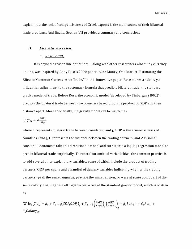
gravity model of trade. Before Rose, the economic model (developed by Tinbergen (1962))
predicts the bilateral trade between two countries based off of the product of GDP and their
distance apart. More specifically, the gravity model can be written as
(1)𝑇𝑖𝑗 = 𝐴 𝐺𝐷𝑃𝑖𝑗𝐷𝑖𝑗
,
where T represents bilateral trade between countries i and j, GDP is the economic mass of
countries i and j, D represents the distance between the trading partners, and A is some
constant. Economists take this “traditional” model and turn it into a log-log regression model to
predict bilateral trade empirically. To control for omitted variable bias, the common practice is
to add several other explanatory variables, some of which include the product of trading
partners’ GDP per capita and a handful of dummy variables indicating whether the trading
partners speak the same language, practice the same religion, or were at some point part of the
same colony. Putting these all together we arrive at the standard gravity model, which is written
as
(2) log�𝑇𝑖𝑗𝑡� = 𝛽0 + 𝛽1 log�𝐺𝐷𝑃𝑖𝐺𝐷𝑃𝑗�𝑡 + 𝛽2 log��𝐺𝐷𝑃𝑃𝑜𝑝
�𝑖�𝐺𝐷𝑃𝑃𝑜𝑝
�𝑗�𝑡
+ 𝛽3𝐿𝑎𝑛𝑔𝑖𝑗 + 𝛽4𝑅𝑒𝑙𝑖𝑗 +
𝛽5𝐶𝑜𝑙𝑜𝑛𝑦𝑖𝑗.

Matsiras 4
While the common method to estimate these βs is with a time series approach3, Rose instead
does a cross-section. However, regardless of the method, Rose was revolutionary simply because
he added ONE additional dummy variable to regression (2), which he called CU, taking a value
of 1 if both countries share the same currency. To that effect, he finds in his cross sectional data
regression that being in a currency union should increase trade between common currency
partners by around 3 times. This paper, though, was focused on general currency unions over a
period of 30 years – not to how the Rose effect specifically affected countries adopting the euro.
b. Micco, Stein, and Ordonez (2003)
Rose’s research consequently led to a large group of papers in the next decade which
focused specifically on how the euro will affect trade for Eurozone countries.4 One of these
papers, specifically Micco, Stein, and Ordonez (2003), quickly became the second most
influential paper for my research. Contrary to Rose’s cross sectional dataset, the three authors
employ panel trade data from the IMF’s Direction of Trade Statistics (DOTS) between the years
1992 to 2002. Rather than pursue a cross-sectional dataset to estimate the euro effect, the
authors use a country-pair fixed effects version of the standard gravity model. Using this
technique considerably condenses the information needed since the distance between two
trading countries, the language used, etc., do not change over time and will get absorbed in the
country fixed effect). Regression (2), consequently, can be transformed into a fixed effects model
with the inclusion of α as appears in regression (3).5
(3) log�𝑇𝑖𝑗� = 𝛽0 + 𝛽1 log�𝐺𝐷𝑃𝑖𝐺𝐷𝑃𝑗� + 𝛽2 log��𝐺𝐷𝑃𝑃𝑜𝑝
�𝑖�𝐺𝐷𝑃𝑃𝑜𝑝
�𝑗�+ 𝛼𝑖𝑗.
3 Like the panel estimation I will do later. 4 The greater majority of these papers are summarized very nicely in Baldwin (2006), of which I am very thankful. 5 Regardless of which of the two models used, both for the most part garner the same estimates of the coefficients of interest.
Matsiras 5
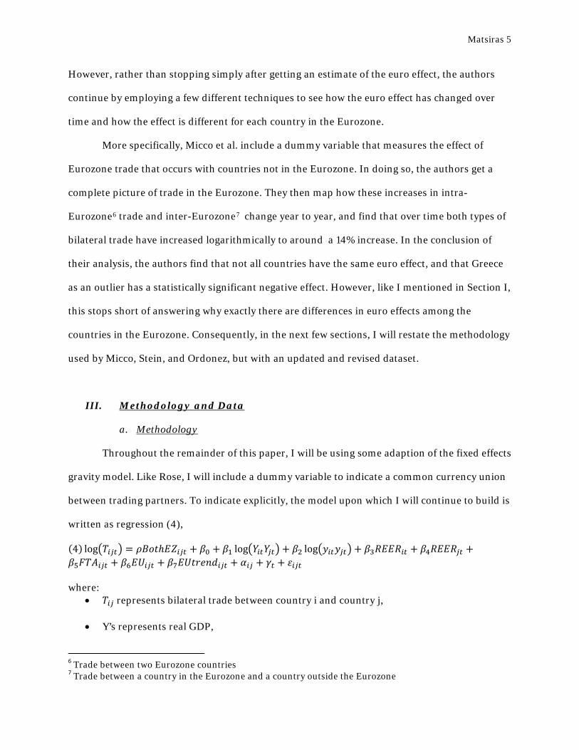
However, rather than stopping simply after getting an estimate of the euro effect, the authors
continue by employing a few different techniques to see how the euro effect has changed over
time and how the effect is different for each country in the Eurozone.
More specifically, Micco et al. include a dummy variable that measures the effect of
Eurozone trade that occurs with countries not in the Eurozone. In doing so, the authors get a
complete picture of trade in the Eurozone. They then map how these increases in intra-
Eurozone6 trade and inter-Eurozone7 change year to year, and find that over time both types of
bilateral trade have increased logarithmically to around a 14% increase. In the conclusion of
their analysis, the authors find that not all countries have the same euro effect, and that Greece
as an outlier has a statistically significant negative effect. However, like I mentioned in Section I,
this stops short of answering why exactly there are differences in euro effects among the
countries in the Eurozone. Consequently, in the next few sections, I will restate the methodology
used by Micco, Stein, and Ordonez, but with an updated and revised dataset.
III. Methodology and Data
a. Methodology
Throughout the remainder of this paper, I will be using some adaption of the fixed effects
gravity model. Like Rose, I will include a dummy variable to indicate a common currency union
between trading partners. To indicate explicitly, the model upon which I will continue to build is
written as regression (4),
(4) log�𝑇𝑖𝑗𝑡� = 𝜌𝐵𝑜𝑡ℎ𝐸𝑍𝑖𝑗𝑡 + 𝛽0 + 𝛽1 log�𝑌𝑖𝑡𝑌𝑗𝑡� + 𝛽2 log�𝑦𝑖𝑡𝑦𝑗𝑡� + 𝛽3𝑅𝐸𝐸𝑅𝑖𝑡 + 𝛽4𝑅𝐸𝐸𝑅𝑗𝑡 +𝛽5𝐹𝑇𝐴𝑖𝑗𝑡 + 𝛽6𝐸𝑈𝑖𝑗𝑡 + 𝛽7𝐸𝑈𝑡𝑟𝑒𝑛𝑑𝑖𝑗𝑡 + 𝛼𝑖𝑗 + 𝛾𝑡 + 𝜀𝑖𝑗𝑡 where:
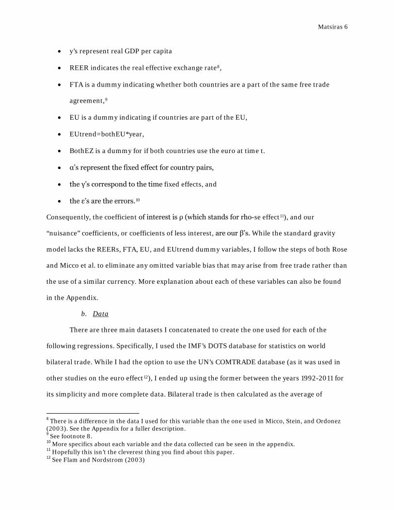
• 𝑇𝑖𝑗 represents bilateral trade between country i and country j,
• Y’s represents real GDP,
6 Trade between two Eurozone countries 7 Trade between a country in the Eurozone and a country outside the Eurozone
Matsiras 6
• y’s represent real GDP per capita
• REER indicates the real effective exchange rate8,
• FTA is a dummy indicating whether both countries are a part of the same free trade
agreement,9
• EU is a dummy indicating if countries are part of the EU,
• EUtrend=bothEU*year,
• BothEZ is a dummy for if both countries use the euro at time t.
• α’s represent the fixed effect for country pairs,
• the γ’s correspond to the time fixed effects, and
• the ε’s are the errors.10
Consequently, the coefficient of interest is ρ (which stands for rho-se effect11), and our
“nuisance” coefficients, or coefficients of less interest, are our β’s. While the standard gravity
model lacks the REERs, FTA, EU, and EUtrend dummy variables, I follow the steps of both Rose
and Micco et al. to eliminate any omitted variable bias that may arise from free trade rather than
the use of a similar currency. More explanation about each of these variables can also be found
in the Appendix.
b. Data
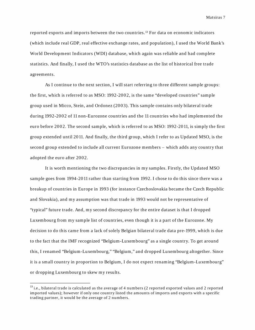
There are three main datasets I concatenated to create the one used for each of the
following regressions. Specifically, I used the IMF’s DOTS database for statistics on world
bilateral trade. While I had the option to use the UN’s COMTRADE database (as it was used in
other studies on the euro effect12), I ended up using the former between the years 1992-2011 for
its simplicity and more complete data. Bilateral trade is then calculated as the average of
8 There is a difference in the data I used for this variable than the one used in Micco, Stein, and Ordonez (2003). See the Appendix for a fuller description. 9 See footnote 8. 10 More specifics about each variable and the data collected can be seen in the appendix. 11 Hopefully this isn’t the cleverest thing you find about this paper. 12 See Flam and Nordstrom (2003)
Matsiras 7
reported exports and imports between the two countries.13 For data on economic indicators
(which include real GDP, real effective exchange rates, and population), I used the World Bank’s
World Development Indicators (WDI) database, which again was reliable and had complete
statistics. And finally, I used the WTO’s statistics database as the list of historical free trade
agreements.
As I continue to the next section, I will start referring to three different sample groups:
the first, which is referred to as MSO: 1992-2002, is the same “developed countries” sample
group used in Micco, Stein, and Ordonez (2003). This sample contains only bilateral trade
during 1992-2002 of 11 non-Eurozone countries and the 11 countries who had implemented the
euro before 2002. The second sample, which is referred to as MSO: 1992-2011, is simply the first
group extended until 2011. And finally, the third group, which I refer to as Updated MSO, is the
second group extended to include all current Eurozone members – which adds any country that
adopted the euro after 2002.
It is worth mentioning the two discrepancies in my samples. Firstly, the Updated MSO
sample goes from 1994-2011 rather than starting from 1992. I chose to do this since there was a
breakup of countries in Europe in 1993 (for instance Czechoslovakia became the Czech Republic
and Slovakia), and my assumption was that trade in 1993 would not be representative of
“typical” future trade. And, my second discrepancy for the entire dataset is that I dropped
Luxembourg from my sample list of countries, even though it is a part of the Eurozone. My
decision to do this came from a lack of solely Belgian bilateral trade data pre-1999, which is due
to the fact that the IMF recognized “Belgium-Luxembourg” as a single country. To get around
this, I renamed “Belgium-Luxembourg,” “Belgium,” and dropped Luxembourg altogether. Since
it is a small country in proportion to Belgium, I do not expect renaming “Belgium-Luxembourg”
or dropping Luxembourg to skew my results.
13 i.e., bilateral trade is calculated as the average of 4 numbers (2 reported exported values and 2 reported imported values); however if only one country listed the amounts of imports and exports with a specific trading partner, it would be the average of 2 numbers.

Matsiras 8
But in summary, the benefit from having these three groups will be to (a) see how the
Micco, Stein, and Ordonez paper would have looked both with my dataset and then extended
until 2011, and (b) see how the newest members to the Eurozone influence the overall euro
effect. More specific information regarding the data, the complete list of countries used in each
sample, and list of free trade agreements can be read in the Appendix.
IV. Calculating the Euro Effect Empirically
a. First Impressions
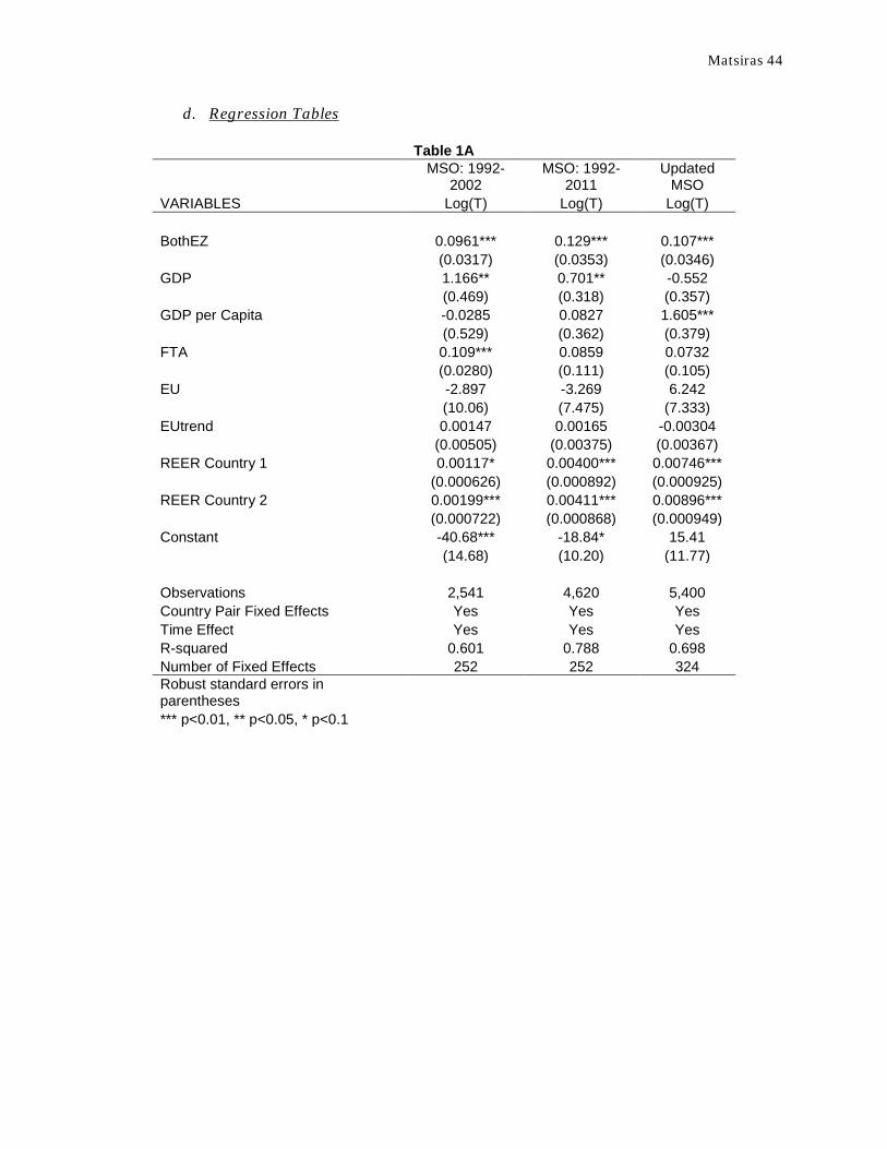
A good place to start is by running the simplest version of the fixed effect gravity model
with a currency union dummy variable like regression (4). Table 1A displays (as well as the
majority of the following tables) three different columns of regression results, with each column
referring to one of the sample groups explained in the previous section.
Table 1A
MSO: 1992-
2002 MSO: 1992-
2011 Updated
MSO VARIABLES Log(T) Log(T) Log(T) BothEZ 0.0961*** 0.129*** 0.107***
(0.0317) (0.0353) (0.0346)
GDP 1.166** 0.701** -0.552
(0.469) (0.318) (0.357)
GDP per Capita -0.0285 0.0827 1.605***
(0.529) (0.362) (0.379)
FTA 0.109*** 0.0859 0.0732
(0.0280) (0.111) (0.105)
EU -2.897 -3.269 6.242
(10.06) (7.475) (7.333)
EUtrend 0.00147 0.00165 -0.00304
(0.00505) (0.00375) (0.00367)
REER Country 1 0.00117* 0.00400*** 0.00746***
(0.000626) (0.000892) (0.000925)
REER Country 2 0.00199*** 0.00411*** 0.00896***
(0.000722) (0.000868) (0.000949)
Constant -40.68*** -18.84* 15.41
(14.68) (10.20) (11.77)
Observations 2,541 4,620 5,400 Country Pair Fixed Effects Yes Yes Yes Time Effect Yes Yes Yes
Matsiras 9
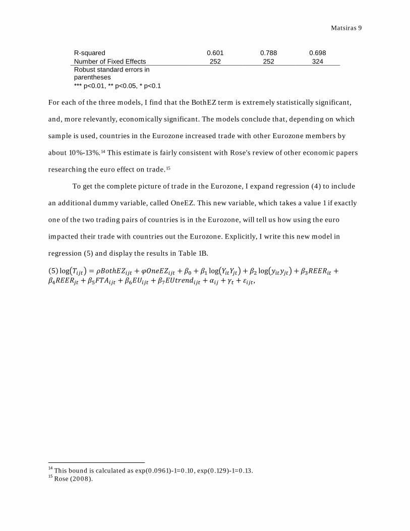
R-squared 0.601 0.788 0.698 Number of Fixed Effects 252 252 324 Robust standard errors in parentheses
*** p<0.01, ** p<0.05, * p<0.1
For each of the three models, I find that the BothEZ term is extremely statistically significant,
and, more relevantly, economically significant. The models conclude that, depending on which
sample is used, countries in the Eurozone increased trade with other Eurozone members by
about 10%-13%.14 This estimate is fairly consistent with Rose's review of other economic papers
researching the euro effect on trade.15
To get the complete picture of trade in the Eurozone, I expand regression (4) to include
an additional dummy variable, called OneEZ. This new variable, which takes a value 1 if exactly
one of the two trading pairs of countries is in the Eurozone, will tell us how using the euro
impacted their trade with countries out the Eurozone. Explicitly, I write this new model in
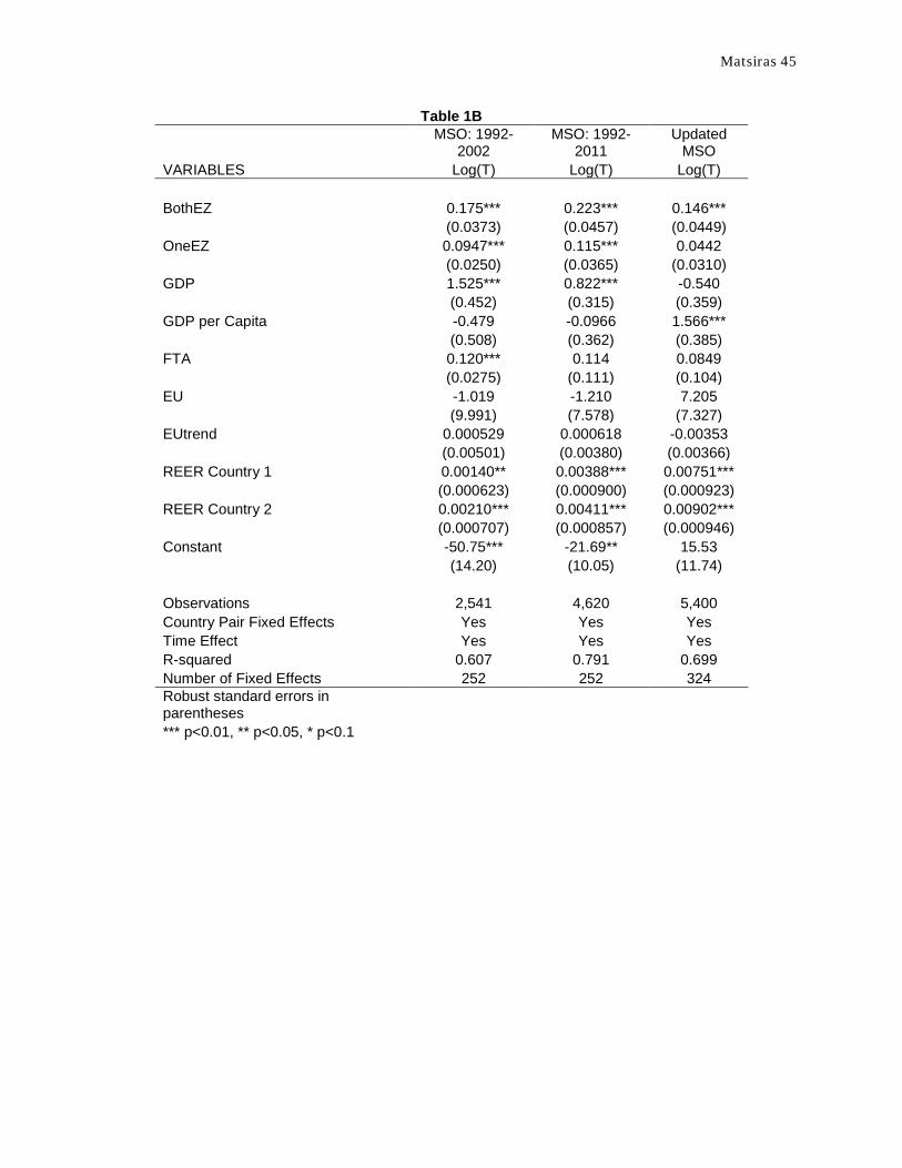
regression (5) and display the results in Table 1B.
(5) log�𝑇𝑖𝑗𝑡� = 𝜌𝐵𝑜𝑡ℎ𝐸𝑍𝑖𝑗𝑡 + 𝜑𝑂𝑛𝑒𝐸𝑍𝑖𝑗𝑡 + 𝛽0 + 𝛽1 log�𝑌𝑖𝑡𝑌𝑗𝑡�+ 𝛽2 log�𝑦𝑖𝑡𝑦𝑗𝑡� + 𝛽3𝑅𝐸𝐸𝑅𝑖𝑡 +𝛽4𝑅𝐸𝐸𝑅𝑗𝑡 + 𝛽5𝐹𝑇𝐴𝑖𝑗𝑡 + 𝛽6𝐸𝑈𝑖𝑗𝑡 + 𝛽7𝐸𝑈𝑡𝑟𝑒𝑛𝑑𝑖𝑗𝑡 + 𝛼𝑖𝑗 + 𝛾𝑡 + 𝜀𝑖𝑗𝑡,
14 This bound is calculated as exp(0.0961)-1=0.10, exp(0.129)-1=0.13. 15 Rose (2008).

Matsiras 10
Table 1B
MSO: 1992-
2002 MSO: 1992-
2011 Updated
MSO VARIABLES Log(T) Log(T) Log(T) BothEZ 0.175*** 0.223*** 0.146***
(0.0373) (0.0457) (0.0449)
OneEZ 0.0947*** 0.115*** 0.0442
(0.0250) (0.0365) (0.0310)
GDP 1.525*** 0.822*** -0.540
(0.452) (0.315) (0.359)
GDP per Capita -0.479 -0.0966 1.566***
(0.508) (0.362) (0.385)
FTA 0.120*** 0.114 0.0849
(0.0275) (0.111) (0.104)
EU -1.019 -1.210 7.205
(9.991) (7.578) (7.327)
EUtrend 0.000529 0.000618 -0.00353
(0.00501) (0.00380) (0.00366)
REER Country 1 0.00140** 0.00388*** 0.00751***
(0.000623) (0.000900) (0.000923)
REER Country 2 0.00210*** 0.00411*** 0.00902***
(0.000707) (0.000857) (0.000946)
Constant -50.75*** -21.69** 15.53
(14.20) (10.05) (11.74)
Observations 2,541 4,620 5,400 Country Pair Fixed Effects Yes Yes Yes Time Effect Yes Yes Yes R-squared 0.607 0.791 0.699 Number of Fixed Effects 252 252 324 Robust standard errors in parentheses
*** p<0.01, ** p<0.05, * p<0.1
One noticeable consequence of adding the OneEZ variable is how the coefficient of BothEZ has
dramatically increased for each of the different samples. For instance in the third sample group,
we have increased our estimate for changes in intra-Eurozone trade from an increase of about
11% to an increase of about 16%.16 The most striking changes in the estimate of the BothEZ
coefficient appear in the results from the second sample group, where the estimate of the
increase in intra-Eurozone trade grew from around 14% to 25%!17
16 These values are calculated as [exp(0.107)-1]*100=11.29, [exp(0.146)-1]*100=15.7. 17 These values are calculated as [exp(0.129)-1]*100=13.77, [exp(0.223)-1]*100=24.98.

Matsiras 11
A few other recognizable consequences occur while comparing the three samples. First,
there is a dramatic increase in BothEZ and OneEZ effects from switching from the MSO: 1992-
2002 sample to the MSO:1992-2011 sample. The results suggest that with the extension of time,
the earliest adopters of the euro have benefited even more by being in the Eurozone. Specifically,
intra-Eurozone trade has increased from around 19% to 25%, and inter-Eurozone trade has
increased from 10% to 12%.
The last fairly recognizable conclusions drawn from Table 1B come from the differences
between the MSO sample group and the Updated MSO sample group. While the first two sample
groups have a statistically significant and positive OneEZ coefficient, the third sample group has
a statistically insignificant effect of OneEZ trade. This could indicate that the more recent
Eurozone members have not taken full advantage of their currency with trading partners outside
the Eurozone and has caused the coefficient to be insignificant. Along those lines, we see that
the estimate of the coefficient for GDP is positive and statistically significant in the first two
sample groups, but not in the third. The reverse is also true when looking at the estimate of the
coefficient for GDP per capita. While unusual, these results suggest that the income per person
was more important for the newest members to the Eurozone, rather than simply the GDP of the
country as a whole.
b. Trend Over Time
Regressions (4) and (5) have given us a good introduction to thinking about the euro
effect, but they left out a crucial component in which we are very interested: how the euro effect
changed over time. There are three ways to measure how the euro effect changes over time. The
first method is specifically used in Micco, Stein, and Ordonez (2003). During their analysis of
the trend of the euro effect, the authors made 9 interaction terms between EMU2 (which is 1 if

Matsiras 12
the pair of countries are both in or will be in the Eurozone18) and an indicator variable for the
years 1993-2002. The model can be written as
(6) log�𝑇𝑖𝑗𝑡� = ∑ 𝜌𝑡𝐸𝑀𝑈2𝑖𝑗𝐼(𝑘 = 𝑡)2011𝑘=1992 + 𝛽0 + 𝛽1 log�𝑌𝑖𝑡𝑌𝑗𝑡�+ 𝛽2 log�𝑦𝑖𝑡𝑦𝑗𝑡� + 𝛽3𝑅𝐸𝐸𝑅𝑖𝑡 +
𝛽4𝑅𝐸𝐸𝑅𝑗𝑡 + 𝛽5𝐹𝑇𝐴𝑖𝑗𝑡 + 𝛽6𝐸𝑈𝑖𝑗𝑡 + 𝛽7𝐸𝑈𝑡𝑟𝑒𝑛𝑑𝑖𝑗𝑡 + 𝛼𝑖𝑗 + 𝛾𝑡 + 𝜀𝑖𝑗𝑡. The authors’ reasoning behind creating such an EMU2 term is to see in precisely which year
there was a significant euro effect. Once running regression (6), the authors find that the euro
effect started being significant in1998 (as shown in their regression results posted below in
Table 2).
18 For instance, EMU2=1 if the countries are Greece and Germany and year is 1995, even though the euro was not in use.
Source: Micco, Stein, and Ordonez (2003)

Matsiras 13
However, as Table 2A in the appendix shows, if we extend the sample out to 2011, we completely
lose the significance of the EMU2-1998 term. Figure 2A plots in a normalized way the estimates
of EMU2 coefficients by year (with the 95% confidence interval being within the dashed lines).
Using the MSO:1992-2011 sample, I find that the estimate of the euro effect becomes positive
starting in 1999, and significantly positive after 2002. This would then negate the claim made in
Micco, Stein, and Ordonez, and instead conclude that the euro effect appears first in the year it
was implemented.
Since it turned out that the Micco, Stein, and Ordonez paper method of measuring the
euro effect over time was not significant during the pre-euro era, we can condense it into the
second version: creating an interaction between BothEZ and an indicator of the year going from
2000-2011 (BothEZ-1999 is omitted because of the dummy variable trap). The regression below
gives more detail of the model.
(7) log�𝑇𝑖𝑗𝑡� = ∑ 𝜌𝑡𝐵𝑜𝑡ℎ𝐸𝑍𝑖𝑗𝐼(𝑘 = 𝑡)2011𝑘=1999 + 𝛽0 + 𝛽1 log�𝑌𝑖𝑡𝑌𝑗𝑡�+ 𝛽2 log�𝑦𝑖𝑡𝑦𝑗𝑡�+ 𝛽3𝑅𝐸𝐸𝑅𝑖𝑡 +
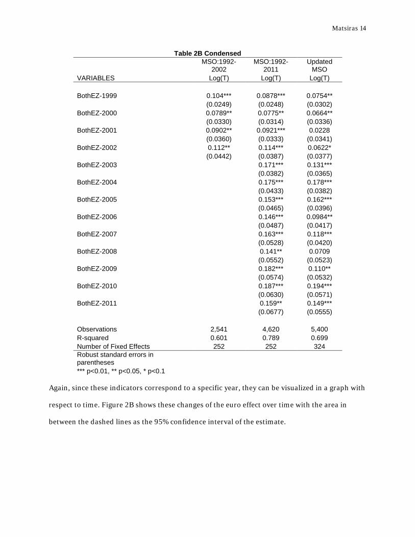
𝛽4𝑅𝐸𝐸𝑅𝑗𝑡 + 𝛽5𝐹𝑇𝐴𝑖𝑗𝑡 + 𝛽6𝐸𝑈𝑖𝑗𝑡 + 𝛽7𝐸𝑈𝑡𝑟𝑒𝑛𝑑𝑖𝑗𝑡 + 𝛼𝑖𝑗 + 𝛾𝑡 + 𝜀𝑖𝑗𝑡 While Table 2B in the Appendix shows the results from the entire regression, the key coefficient
estimates are reproduced below in Table 2B Condensed.
-30
-20
-10
0
10
20
30
40
1993
1994
1995
1996
1997
1998
1999
2000
2001
2002
2003
2004
2005
2006
2007
2008
2009
2010
2011
% In
crea
se in
Bila
tera
l Tra
de
Year
Figure 2A
EMU2 Effect
95% Confidence Interval
Matsiras 14
Table 2B Condensed
MSO:1992-
2002 MSO:1992-
2011 Updated
MSO VARIABLES Log(T) Log(T) Log(T) BothEZ-1999 0.104*** 0.0878*** 0.0754**
(0.0249) (0.0248) (0.0302)
BothEZ-2000 0.0789** 0.0775** 0.0664**
(0.0330) (0.0314) (0.0336)
BothEZ-2001 0.0902** 0.0921*** 0.0228
(0.0360) (0.0333) (0.0341)
BothEZ-2002 0.112** 0.114*** 0.0622*
(0.0442) (0.0387) (0.0377)
BothEZ-2003
0.171*** 0.131***
(0.0382) (0.0365)
BothEZ-2004
0.175*** 0.178***
(0.0433) (0.0382)
BothEZ-2005
0.153*** 0.162***
(0.0465) (0.0396)
BothEZ-2006
0.146*** 0.0984**
(0.0487) (0.0417)
BothEZ-2007
0.163*** 0.118***
(0.0528) (0.0420)
BothEZ-2008
0.141** 0.0709
(0.0552) (0.0523)
BothEZ-2009
0.182*** 0.110**
(0.0574) (0.0532)
BothEZ-2010
0.187*** 0.194***
(0.0630) (0.0571)
BothEZ-2011
0.159** 0.149***
(0.0677) (0.0555)
Observations 2,541 4,620 5,400 R-squared 0.601 0.789 0.699 Number of Fixed Effects 252 252 324 Robust standard errors in parentheses
*** p<0.01, ** p<0.05, * p<0.1
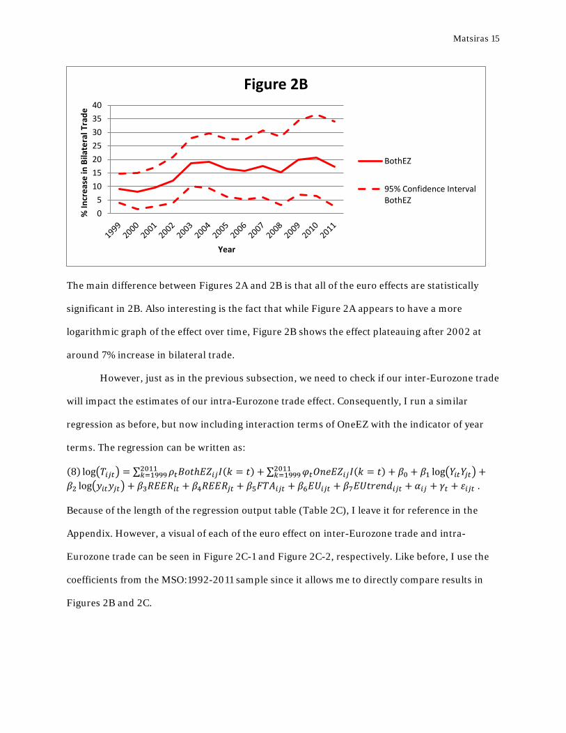
Again, since these indicators correspond to a specific year, they can be visualized in a graph with
respect to time. Figure 2B shows these changes of the euro effect over time with the area in
between the dashed lines as the 95% confidence interval of the estimate.
Matsiras 15
The main difference between Figures 2A and 2B is that all of the euro effects are statistically
significant in 2B. Also interesting is the fact that while Figure 2A appears to have a more
logarithmic graph of the effect over time, Figure 2B shows the effect plateauing after 2002 at
around 7% increase in bilateral trade.
However, just as in the previous subsection, we need to check if our inter-Eurozone trade
will impact the estimates of our intra-Eurozone trade effect. Consequently, I run a similar
regression as before, but now including interaction terms of OneEZ with the indicator of year
terms. The regression can be written as:
(8) log�𝑇𝑖𝑗𝑡� = ∑ 𝜌𝑡𝐵𝑜𝑡ℎ𝐸𝑍𝑖𝑗𝐼(𝑘 = 𝑡)2011𝑘=1999 + ∑ 𝜑𝑡𝑂𝑛𝑒𝐸𝑍𝑖𝑗𝐼(𝑘 = 𝑡)2011
𝑘=1999 + 𝛽0 + 𝛽1 log�𝑌𝑖𝑡𝑌𝑗𝑡� +𝛽2 log�𝑦𝑖𝑡𝑦𝑗𝑡� + 𝛽3𝑅𝐸𝐸𝑅𝑖𝑡 + 𝛽4𝑅𝐸𝐸𝑅𝑗𝑡 + 𝛽5𝐹𝑇𝐴𝑖𝑗𝑡 + 𝛽6𝐸𝑈𝑖𝑗𝑡 + 𝛽7𝐸𝑈𝑡𝑟𝑒𝑛𝑑𝑖𝑗𝑡 + 𝛼𝑖𝑗 + 𝛾𝑡 + 𝜀𝑖𝑗𝑡 . Because of the length of the regression output table (Table 2C), I leave it for reference in the
Appendix. However, a visual of each of the euro effect on inter-Eurozone trade and intra-
Eurozone trade can be seen in Figure 2C-1 and Figure 2C-2, respectively. Like before, I use the
coefficients from the MSO:1992-2011 sample since it allows me to directly compare results in
Figures 2B and 2C.
05
10152025303540
% In
crea
se in
Bila
tera
l Tra
de
Year
Figure 2B
BothEZ
95% Confidence IntervalBothEZ

Matsiras 16
There is quite a bit to interpret from these two Figures: namely, countries who adopted the euro
before 2002 have now increased intra-Eurozone trade by 30% and inter-Eurozone trade by
around 10-20%! This is extremely large compared to results found in other papers. However, my
results do stay consistent as those in Table 1B, since the BothEZ effects are higher than the effect
of OneEZ.
Focusing in on Figure 2C – 1, one can see that inter-Eurozone trade has had a more
cyclical pattern as time progresses, since the effect shoots up to around 20% increase of trade,
wobbles down to 10%, and then picks back up towards 13% in 2011 (however, after around
-10
0
10
20
30
40
50
60
70
% In
crea
se in
Bila
tera
l Tra
de
Year
Figure 2C - 1
OneEZ
95% Confidence IntervalOneEZ
-10
0
10
20
30
40
50
60
70
% In
crea
se in
Bila
tera
l Tra
de
Year
Figure 2C - 2
BothEZ
95% Confidence IntervalBothEZ
Matsiras 17
2008, the estimates stop being significant). This is much less the case for intra-Eurozone trade,
which shows bilateral trade increasing to around 35%, and then plateauing (as it plateaued in
Figure 2A) to an increase of around 30%. One can feel more confident about the estimates for
the BothEZ coefficient, since the 95% confidence interval for the estimate of BothEZ never
reaches 0% during the 1999-2011 period.
While the past few regressions have been convenient (since I can actually graph specific
values), the third and final method to measure the euro effect over time is the simplest: an
interaction of BothEZ*year and OneEZ*year. This is inherently appropriate since the
regressions are shorter, but still control for how the euro effect changes over time. The
regression specifies the model, and Table 2E shows the results:
(9) log�𝑇𝑖𝑗� = 𝜌�𝐵𝑜𝑡ℎ𝐸𝑍𝑖𝑗𝑡 ∗ 𝑡� + 𝜑�𝑂𝑛𝑒𝐸𝑍𝑖𝑗𝑡 ∗ 𝑡� + 𝛽0 + 𝛽1 log�𝑌𝑖𝑌𝑗� + 𝛽2 log�𝑦𝑖𝑡𝑦𝑗𝑡� +𝛽3𝑅𝐸𝐸𝑅𝑖𝑡 + 𝛽4𝑅𝐸𝐸𝑅𝑗𝑡 + 𝛽5𝐹𝑇𝐴𝑖𝑗𝑡 + 𝛽6𝐸𝑈𝑖𝑗𝑡 + 𝛽7𝐸𝑈𝑡𝑟𝑒𝑛𝑑𝑖𝑗𝑡 + 𝛼𝑖𝑗 + 𝛾𝑡 + 𝜀𝑖𝑗𝑡
Table 2D
MSO:1992-
2002 MSO:1992-
2011 Updated
MSO VARIABLES Log(T) Log(T) Log(T) BothEZ*t 8.73e-05*** 0.000111*** 7.29e-05***
(1.87e-05) (2.29e-05) (2.24e-05)
OneEZ*t 4.74e-05*** 5.72e-05*** 2.20e-05
(1.25e-05) (1.82e-05) (1.55e-05)
GDP 1.525*** 0.822*** -0.540
(0.452) (0.315) (0.358)
GDP per Capita -0.479 -0.0965 1.567***
(0.508) (0.362) (0.385)
FTA 0.120*** 0.115 0.0850
(0.0275) (0.111) (0.104)
EU -1.009 -1.144 7.257
(9.992) (7.584) (7.329)
EUtrend 0.000524 0.000585 -0.00355
(0.00501) (0.00380) (0.00366)
REER Country 1 0.00140** 0.00388*** 0.00751***
(0.000623) (0.000901) (0.000923)
REER Country 2 0.00210*** 0.00411*** 0.00902***
(0.000707) (0.000857) (0.000946)
Constant -50.75*** -21.69** 15.53
(14.20) (10.05) (11.74)
Observations 2,541 4,620 5,400 Country Pair Fixed Effects Yes Yes Yes
Matsiras 18
Time Effects Yes Yes Yes R-squared 0.607 0.792 0.699 Number of Fixed Effects 252 252 324 Robust standard errors in parentheses
*** p<0.01, ** p<0.05, * p<0.1
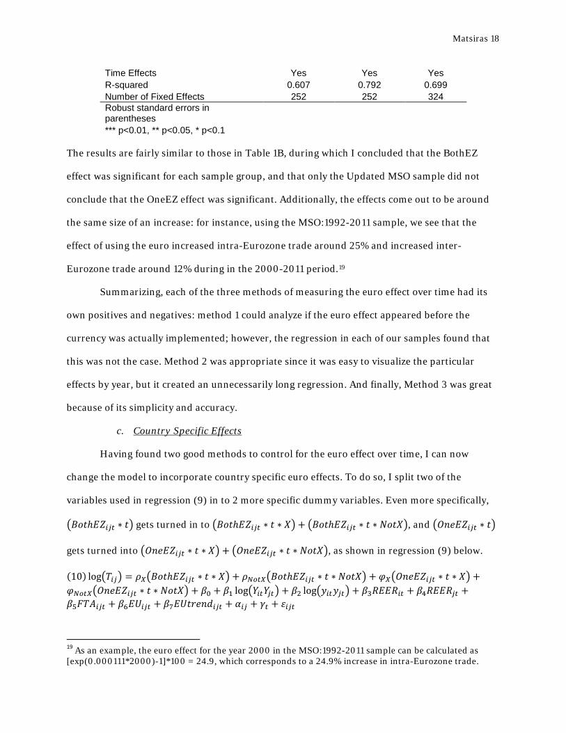
The results are fairly similar to those in Table 1B, during which I concluded that the BothEZ
effect was significant for each sample group, and that only the Updated MSO sample did not
conclude that the OneEZ effect was significant. Additionally, the effects come out to be around
the same size of an increase: for instance, using the MSO:1992-2011 sample, we see that the
effect of using the euro increased intra-Eurozone trade around 25% and increased inter-
Eurozone trade around 12% during in the 2000-2011 period.19
Summarizing, each of the three methods of measuring the euro effect over time had its
own positives and negatives: method 1 could analyze if the euro effect appeared before the
currency was actually implemented; however, the regression in each of our samples found that
this was not the case. Method 2 was appropriate since it was easy to visualize the particular
effects by year, but it created an unnecessarily long regression. And finally, Method 3 was great
because of its simplicity and accuracy.
c. Country Specific Effects
Having found two good methods to control for the euro effect over time, I can now
change the model to incorporate country specific euro effects. To do so, I split two of the
variables used in regression (9) in to 2 more specific dummy variables. Even more specifically,
�𝐵𝑜𝑡ℎ𝐸𝑍𝑖𝑗𝑡 ∗ 𝑡� gets turned in to �𝐵𝑜𝑡ℎ𝐸𝑍𝑖𝑗𝑡 ∗ 𝑡 ∗ 𝑋� + �𝐵𝑜𝑡ℎ𝐸𝑍𝑖𝑗𝑡 ∗ 𝑡 ∗ 𝑁𝑜𝑡𝑋�, and �𝑂𝑛𝑒𝐸𝑍𝑖𝑗𝑡 ∗ 𝑡�
gets turned into �𝑂𝑛𝑒𝐸𝑍𝑖𝑗𝑡 ∗ 𝑡 ∗ 𝑋� + �𝑂𝑛𝑒𝐸𝑍𝑖𝑗𝑡 ∗ 𝑡 ∗ 𝑁𝑜𝑡𝑋�, as shown in regression (9) below.
(10) log�𝑇𝑖𝑗� = 𝜌𝑋�𝐵𝑜𝑡ℎ𝐸𝑍𝑖𝑗𝑡 ∗ 𝑡 ∗ 𝑋� + 𝜌𝑁𝑜𝑡𝑋�𝐵𝑜𝑡ℎ𝐸𝑍𝑖𝑗𝑡 ∗ 𝑡 ∗ 𝑁𝑜𝑡𝑋� + 𝜑𝑋�𝑂𝑛𝑒𝐸𝑍𝑖𝑗𝑡 ∗ 𝑡 ∗ 𝑋� +𝜑𝑁𝑜𝑡𝑋�𝑂𝑛𝑒𝐸𝑍𝑖𝑗𝑡 ∗ 𝑡 ∗ 𝑁𝑜𝑡𝑋� + 𝛽0 + 𝛽1 log�𝑌𝑖𝑡𝑌𝑗𝑡� + 𝛽2 log�𝑦𝑖𝑡𝑦𝑗𝑡� + 𝛽3𝑅𝐸𝐸𝑅𝑖𝑡 + 𝛽4𝑅𝐸𝐸𝑅𝑗𝑡 +𝛽5𝐹𝑇𝐴𝑖𝑗𝑡 + 𝛽6𝐸𝑈𝑖𝑗𝑡 + 𝛽7𝐸𝑈𝑡𝑟𝑒𝑛𝑑𝑖𝑗𝑡 + 𝛼𝑖𝑗 + 𝛾𝑡 + 𝜀𝑖𝑗𝑡
19 As an example, the euro effect for the year 2000 in the MSO:1992-2011 sample can be calculated as [exp(0.000111*2000)-1]*100 = 24.9, which corresponds to a 24.9% increase in intra-Eurozone trade.

Matsiras 19
Here, X represents a dummy variable that takes a value 1 when country X is one of the trading
partners. Likewise, NotX is a dummy variable which takes a value 1 when country X is neither of
the two trading partners. This process should make sense intuitively, since essentially we tell
regression (9) to split the BothEZ*t coefficient into a weighted sum specific to two groups: NotX
and X. It also proves to be a more reliable estimate than say a version of regression (10) that
excludes the NotX dummies.
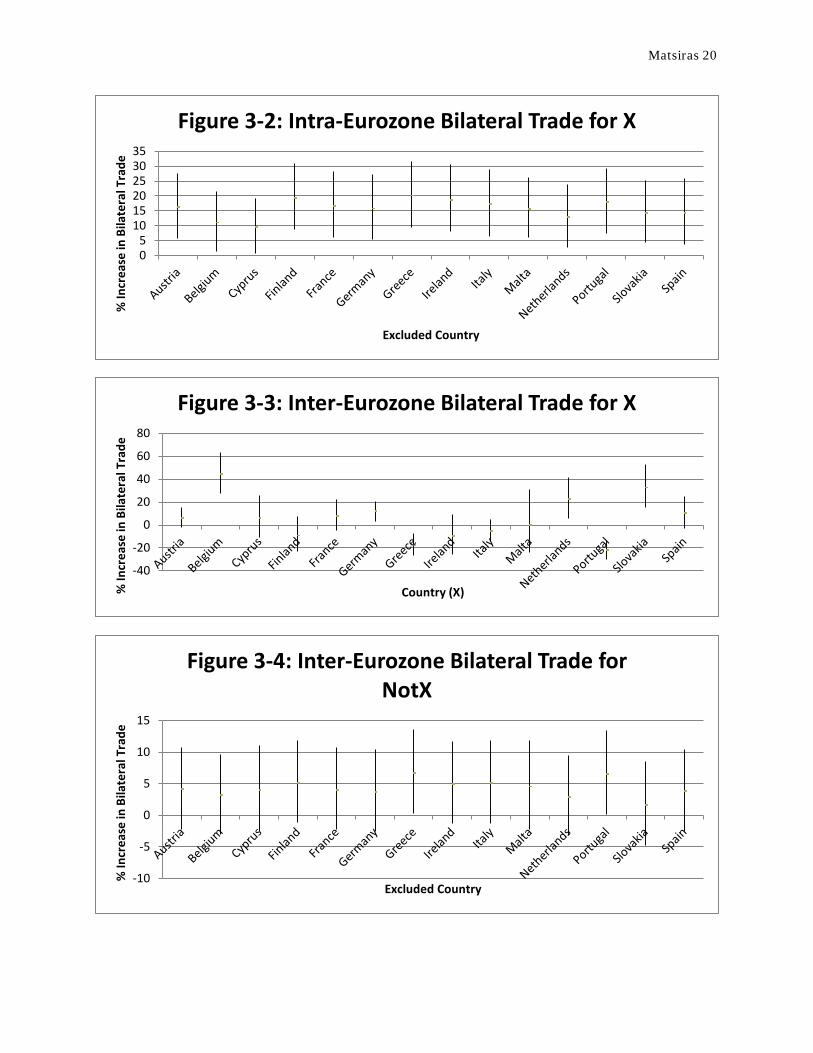
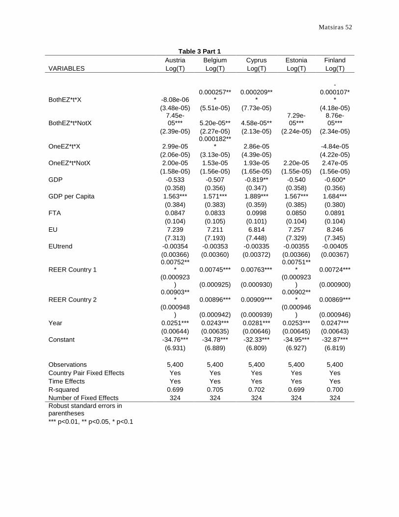
Running this regression 16 times using the Updated MSO sample (once for each country
in the Eurozone), I obtain the results which appear in Table 3 in the Appendix. For reference,
the most relevant results are plotted in the figures below using estimates for 2010.20
20 Please take note of the different Y-axis values.
-60
-40
-20
0
20
40
60
80
100
120
% In
crea
se in
Bila
tera
l Tra
de
Country (X)
Figure 3-1: Intra-Eurozone Bilateral Trade for X
Matsiras 20
05
101520253035
% In
crea
se in
Bila
tera
l Tra
de
Excluded Country
Figure 3-2: Intra-Eurozone Bilateral Trade for X
-40
-20
0
20
40
60
80
% In
crea
se in
Bila
tera
l Tra
de
Country (X)
Figure 3-3: Inter-Eurozone Bilateral Trade for X
-10
-5
0
5
10
15
% In
crea
se in
Bila
tera
l Tra
de
Excluded Country
Figure 3-4: Inter-Eurozone Bilateral Trade for NotX

Matsiras 21
As a note, each graph shows the 95% confidence interval for the estimated percent increase in
bilateral trade for a certain country, X [group of countries, NotX], and a certain region of trading
partners (intra-Eurozone or inter-Eurozone). For example, a correct interpretation of Figure 3-1
would be, “according to Figure 3-1, a 95% confidence interval for the estimated decrease in
intra-Eurozone bilateral trade for Greece is between 10 to 30%.” Likewise, an equally correct
statement about Figure 3-2 would be, “according to Figure 3-2, a 95% confidence interval for the
estimated increase in intra-Eurozone bilateral trade for countries that are not Greece is between
10 to 30%.”
These figures, while giving a good visual of how bilateral trade has changed during the
euro era, do not answer an overlaying question of is intra-Eurozone and inter-Eurozone bilateral
trade the same for whether you are a specific country or not; or, put in the context of regression
(10), is 𝜌𝑥 = 𝜌𝑁𝑜𝑡𝑋 and 𝜑𝑋 = 𝜑𝑁𝑜𝑡𝑋 for each country X? Thankfully, this can be solved quickly
with 16 appropriate series of F-tests with the null hypothesis that the means are equal. The p-
values from the 16*2 F-tests appear in Test Table 3, and provide a good complement to Figures
3-1 to 3-4.
Test Table 3
Country BothEZ*t*X =
BothEZ*t*NotX OneEZ*t*X =
OneEZ*t*NotX Austria 0.093 0.730 Belgium 0.002 0.000 Cyprus 0.055 0.859 Finland 0.000 0.117 France 0.074 0.622
Germany 0.112 0.195 Greece 0.000 0.000 Ireland 0.001 0.151
Italy 0.016 0.116 Malta 0.526 0.770
Netherlands 0.502 0.042 Portugal 0.004 0.000 Slovakia 0.355 0.002
Spain 0.665 0.442
Comparing these results to the figures above, we notice that Greece is an unfortunate
standout from the Eurozone members for the following reasons: both its estimated values of
Matsiras 22
change in bilateral intra-Eurozone trade and inter-Eurozone trade are negative, while
NotGreece has positive effects. Moreover, we can reject a null hypothesis that the estimated
values for Greece and NotGreece are the same at the 1% level.
In summary, we just went through the rigorous process of finding a good way to estimate
the euro effect for the entire Eurozone by year, and specific to countries. We can now specify this
model to Greece and explore the Greek euro effect by year.
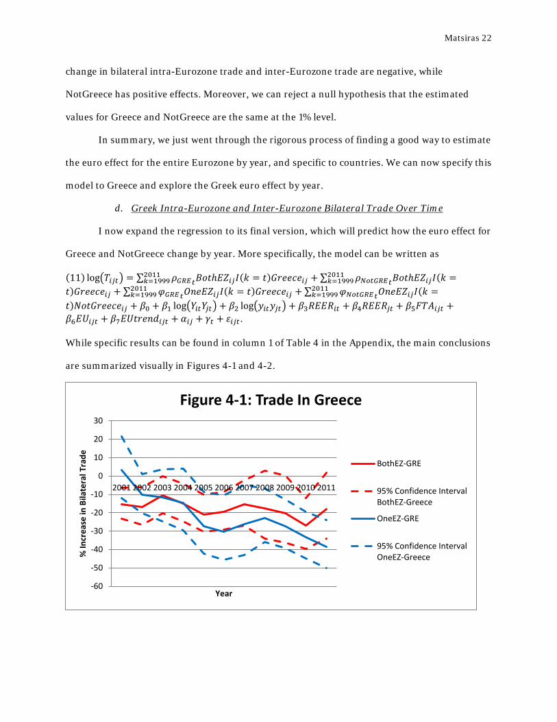
d. Greek Intra-Eurozone and Inter-Eurozone Bilateral Trade Over Time
I now expand the regression to its final version, which will predict how the euro effect for
Greece and NotGreece change by year. More specifically, the model can be written as
(11) log�𝑇𝑖𝑗𝑡� = ∑ 𝜌𝐺𝑅𝐸𝑡𝐵𝑜𝑡ℎ𝐸𝑍𝑖𝑗𝐼(𝑘 = 𝑡)𝐺𝑟𝑒𝑒𝑐𝑒𝑖𝑗2011𝑘=1999 +∑ 𝜌𝑁𝑜𝑡𝐺𝑅𝐸𝑡𝐵𝑜𝑡ℎ𝐸𝑍𝑖𝑗𝐼(𝑘 =2011
𝑘=1999𝑡)𝐺𝑟𝑒𝑒𝑐𝑒𝑖𝑗 + ∑ 𝜑𝐺𝑅𝐸𝑡𝑂𝑛𝑒𝐸𝑍𝑖𝑗𝐼(𝑘 = 𝑡)𝐺𝑟𝑒𝑒𝑐𝑒𝑖𝑗2011
𝑘=1999 +∑ 𝜑𝑁𝑜𝑡𝐺𝑅𝐸𝑡𝑂𝑛𝑒𝐸𝑍𝑖𝑗𝐼(𝑘 =2011𝑘=1999
𝑡)𝑁𝑜𝑡𝐺𝑟𝑒𝑒𝑐𝑒𝑖𝑗 + 𝛽0 + 𝛽1 log�𝑌𝑖𝑡𝑌𝑗𝑡� + 𝛽2 log�𝑦𝑖𝑡𝑦𝑗𝑡� + 𝛽3𝑅𝐸𝐸𝑅𝑖𝑡 + 𝛽4𝑅𝐸𝐸𝑅𝑗𝑡 + 𝛽5𝐹𝑇𝐴𝑖𝑗𝑡 +𝛽6𝐸𝑈𝑖𝑗𝑡 + 𝛽7𝐸𝑈𝑡𝑟𝑒𝑛𝑑𝑖𝑗𝑡 + 𝛼𝑖𝑗 + 𝛾𝑡 + 𝜀𝑖𝑗𝑡. While specific results can be found in column 1 of Table 4 in the Appendix, the main conclusions
are summarized visually in Figures 4-1 and 4-2.
-60
-50
-40
-30
-20
-10
0
10
20
30
2001 2002 2003 2004 2005 2006 2007 2008 2009 2010 2011
% In
crea
se in
Bila
tera
l Tra
de
Year
Figure 4-1: Trade In Greece
BothEZ-GRE
95% Confidence IntervalBothEZ-Greece
OneEZ-GRE
95% Confidence IntervalOneEZ-Greece

Matsiras 23
And, like before, a good complement to Figures 4-1 and 4-2 is Test Table 4, which shows the
11*2 p-values of F-tests by year with the null hypothesis that the estimated Greek effect is the
same as the NotGreece effect.
Test Table 4 t BothEZ*Greece*I(Year=t) = BothEZ*NotGreece*I(Year=t) OneEZ*Greece*I(Year=t) = OneEZ*NotGreece*I(Year=t)
2001 0.004 0.852 2002 0.001 0.025 2003 0.001 0.025 2004 0.000 0.008 2005 0.000 0.001 2006 0.000 0.002 2007 0.001 0.006 2008 0.050 0.022 2009 0.018 0.007 2010 0.000 0.000 2011 0.004 0.000
As one can see in the Figures and confirm in the Test Table, both the OneEZ and BothEZ effect
is much different for Greece than it is for NotGreece. Not only that, but has a statistically
significant negative impact on Greek bilateral trade. One similarity between the Figures 4-1 and
4-2 would be that the BothEZ coefficient is consistently greater than the estimated effect of
-20
-10
0
10
20
30
40
50
60
% In
crea
se in
Bila
tera
l Tra
de
Year
Figure 4-2: Trade in Not Greece
BothEZ-NotGRE
95% Confidence IntervalBothEZ-NotGreece
OneEZ-NotGRE
95% Confidence IntervalOneEZ-NotGreece

Matsiras 24
OneEZ on bilateral trade. However, this makes sense since we have reached the same conclusion
in each of the previous regressions.21
Possibly the most important difference between the two Figures is that there is a
downward trend of the euro effect for Greece, while an upward trend for all countries in the
Eurozone which aren’t Greece. This is the moment to which the paper has been building up, and
now one must ask the question: how is Greece getting worse off by being in the Eurozone? And,
is there a way to change it?
V. The Greek Tragedy: Lack of Competitiveness
The answer to the previous question will soon become undoubtedly clear to be the lack of
competitiveness of Greek exports. There has been a plethora of literature on the how export
performance, commodity makeup, and competitiveness have diminished through the years.
Specifically, the Global Competitiveness Report Series and Athanasoglou, Backinezos, and
Georgiou (2010) highlight country-specific and export-specific problems, respectively.
a. Export-Specific Issues
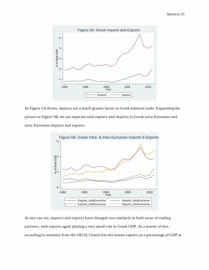
Before getting into the nitty-gritty of Greek exports, it would help to see a visual of how
Greek exports play a role bilateral trade.
21 Another question that could be asked is whether the crisis post 2007 had any significant effects on the Greek Euro effect. However, results in column 2 of Table 4 in the Appendix (during which the years after 2007 were dropped) garner fairly similar, if not slightly lower (more negative) estimates of the Greek euro effect. This would seem to imply that the recessionary period did not have much of an effect on the regression.
Matsiras 25
As Figure 5A shows, imports are a much greater factor in Greek bilateral trade. Expanding the
picture to Figure 5B, we can separate total exports and imports to Greek intra-Eurozone and
inter-Eurozone imports and exports.
As one can see, imports and exports have changed very similarly in both areas of trading
partners, with exports again playing a very small role in Greek GDP. As a matter of fact,
according to statistics from the OECD, Greece has the lowest exports as a percentage of GDP in
.1.2
.3.4
.5%
of R
eal G
DP
1990 1995 2000 2005 2010Year
Exports Imports
Figure 5A: Greek Imports and Exports
0.1
.2.3
% o
f Rea
l GD
P
1990 1995 2000 2005 2010Year
Exports_IntraEurozone Imports_IntraEurozoneExports_InterEurozone Imports_InterEurozone
Figure 5B: Greek Intra- & Inter-Eurozone Imports & Exports
Matsiras 26
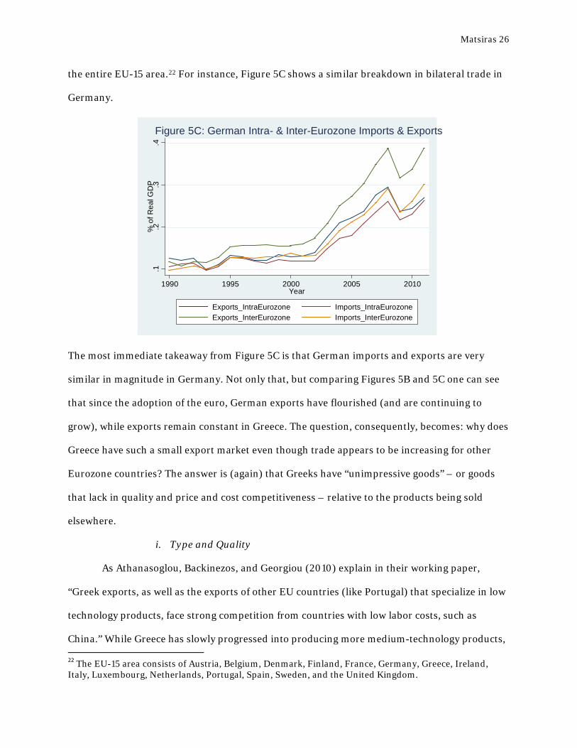
the entire EU-15 area.22 For instance, Figure 5C shows a similar breakdown in bilateral trade in
Germany.
The most immediate takeaway from Figure 5C is that German imports and exports are very
similar in magnitude in Germany. Not only that, but comparing Figures 5B and 5C one can see
that since the adoption of the euro, German exports have flourished (and are continuing to
grow), while exports remain constant in Greece. The question, consequently, becomes: why does
Greece have such a small export market even though trade appears to be increasing for other
Eurozone countries? The answer is (again) that Greeks have “unimpressive goods” – or goods
that lack in quality and price and cost competitiveness – relative to the products being sold
elsewhere.
i. Type and Quality
As Athanasoglou, Backinezos, and Georgiou (2010) explain in their working paper,
“Greek exports, as well as the exports of other EU countries (like Portugal) that specialize in low
technology products, face strong competition from countries with low labor costs, such as
China.” While Greece has slowly progressed into producing more medium-technology products,
22 The EU-15 area consists of Austria, Belgium, Denmark, Finland, France, Germany, Greece, Ireland, Italy, Luxembourg, Netherlands, Portugal, Spain, Sweden, and the United Kingdom.
.1.2
.3.4
% o
f Rea
l GD
P
1990 1995 2000 2005 2010Year
Exports_IntraEurozone Imports_IntraEurozoneExports_InterEurozone Imports_InterEurozone
Figure 5C: German Intra- & Inter-Eurozone Imports & Exports
Matsiras 27
it still has a large proportion of its exports attributed to low-technology products. And,
according to the three authors, Greece produces and exports a limited variety of such products.
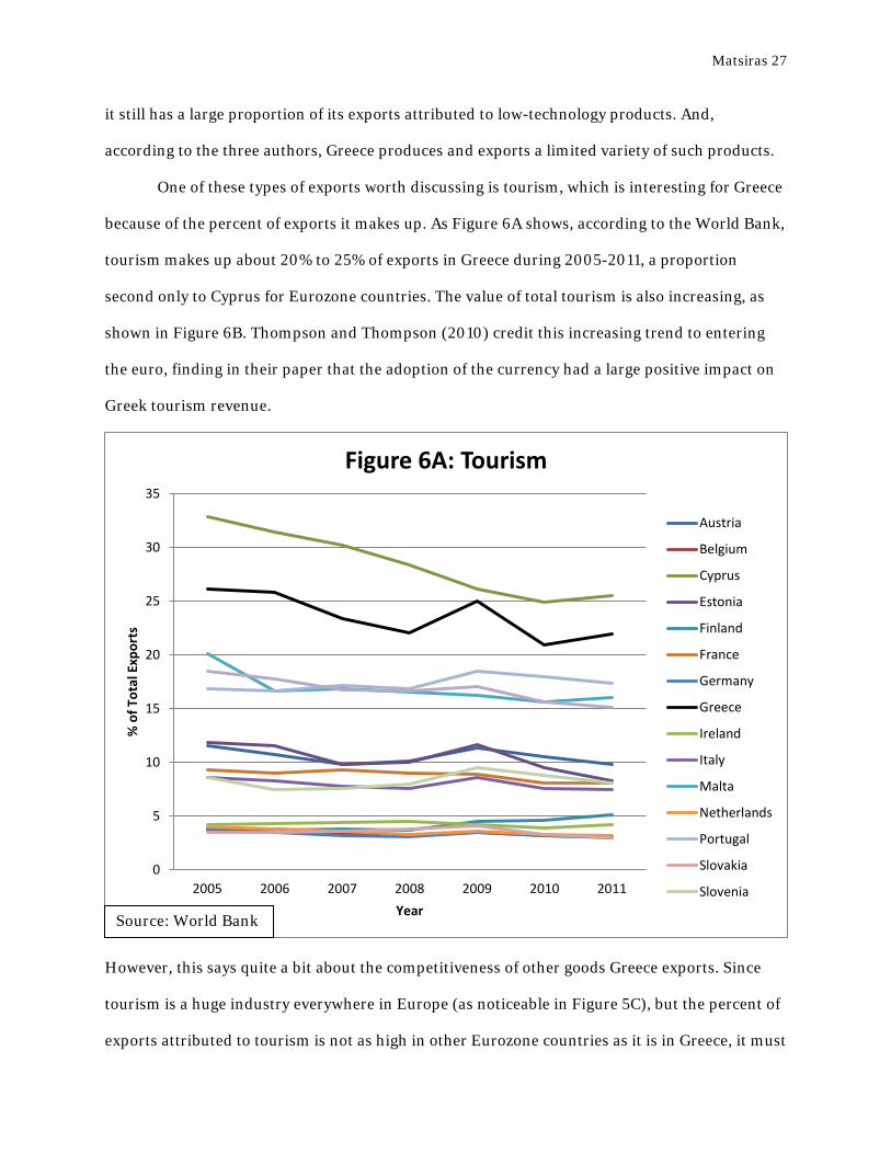
One of these types of exports worth discussing is tourism, which is interesting for Greece
because of the percent of exports it makes up. As Figure 6A shows, according to the World Bank,
tourism makes up about 20% to 25% of exports in Greece during 2005-2011, a proportion
second only to Cyprus for Eurozone countries. The value of total tourism is also increasing, as
shown in Figure 6B. Thompson and Thompson (2010) credit this increasing trend to entering
the euro, finding in their paper that the adoption of the currency had a large positive impact on
Greek tourism revenue.
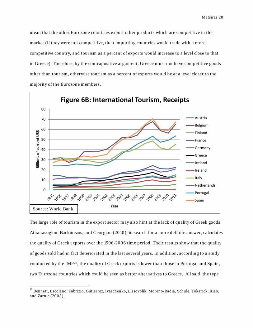
However, this says quite a bit about the competitiveness of other goods Greece exports. Since
tourism is a huge industry everywhere in Europe (as noticeable in Figure 5C), but the percent of
exports attributed to tourism is not as high in other Eurozone countries as it is in Greece, it must
0
5
10
15
20
25
30
35
2005 2006 2007 2008 2009 2010 2011
% o
f Tot
al E
xpor
ts
Year
Figure 6A: Tourism
Austria
Belgium
Cyprus
Estonia
Finland
France
Germany
Greece
Ireland
Italy
Malta
Netherlands
Portugal
Slovakia
Slovenia
Source: World Bank
Matsiras 28
mean that the other Eurozone countries export other products which are competitive in the
market (if they were not competitive, then importing countries would trade with a more
competitive country, and tourism as a percent of exports would increase to a level close to that
in Greece). Therefore, by the contrapositive argument, Greece must not have competitive goods
other than tourism, otherwise tourism as a percent of exports would be at a level closer to the
majority of the Eurozone members.
The large role of tourism in the export sector may also hint at the lack of quality of Greek goods.
Athanasoglou, Backinezos, and Georgiou (2010), in search for a more definite answer, calculates
the quality of Greek exports over the 1996-2006 time period. Their results show that the quality
of goods sold had in fact deteriorated in the last several years. In addition, according to a study
conducted by the IMF23, the quality of Greek exports is lower than those in Portugal and Spain,
two Eurozone countries which could be seen as better alternatives to Greece. All said, the type
23 Bennett, Escolano, Fabrizio, Gutierrez, Ivaschenko, Lissovolik, Moreno-Badia, Schule, Tokarick, Xiao, and Zarnic (2008).
0
10
20
30
40
50
60
70
80
Bill
ions
of c
urre
nt U
S$
Year
Figure 6B: International Tourism, Receipts
Austria
Belgium
Finland
France
Germany
Greece
Iceland
Ireland
Italy
Netherlands
Portugal
Spain
Source: World Bank
Matsiras 29
and quality of exports from Greece plays a significant factor in the lack of competitiveness, and
the lack of improvement after adopting the euro has harshened the negative euro effect.
ii. Price and Cost Competitiveness
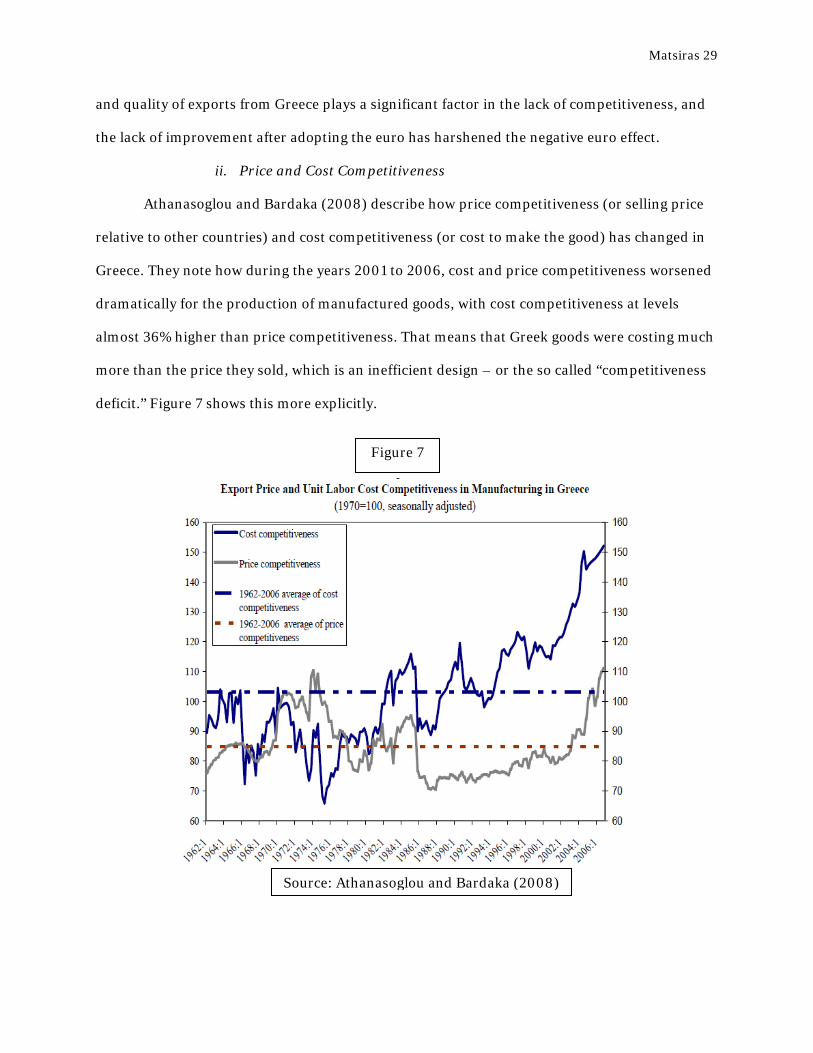
Athanasoglou and Bardaka (2008) describe how price competitiveness (or selling price
relative to other countries) and cost competitiveness (or cost to make the good) has changed in
Greece. They note how during the years 2001 to 2006, cost and price competitiveness worsened
dramatically for the production of manufactured goods, with cost competitiveness at levels
almost 36% higher than price competitiveness. That means that Greek goods were costing much
more than the price they sold, which is an inefficient design – or the so called “competitiveness
deficit.” Figure 7 shows this more explicitly.
Figure 7
Source: Athanasoglou and Bardaka (2008)

Matsiras 30
Consequently, their results discuss the lack of innovation in Greece. For, while prices had
remained somewhat competitive, the manufacturing industry was not able to create more
efficient ways of creating goods. This draws on some of the problems in the Greek labor force,
which is discussed in the next subsection.
b. Country-Specific Issues
Starting in 2006, the World Economic Forum has published the Global Competitiveness
Index (GCI). This index, which rates a country’s competitiveness based on 12 different “pillars”24
then ranks each of the 144 countries in the world. Greece, since the start of this index, has
ranked the lowest in the Eurozone and EU (a visual can be seen in Figure 8). This poor ranking,
as the GCI notes, is due to Greece’s poor macroeconomic environment (where Greece ranks
dead last), and its inefficient labor force, the subjects of the two next subsections.25 The third
subsection describes the differences between trade in Greece and the rest of the Eurozone.
24 http://www.weforum.org/pdf/Global_Competitiveness_Reports/Reports/gcr_2006/chapter_1_1.pdf 25 Naturally it would be interesting to see how including the GCI into the previous regressions would change the magnitude of the euro effect (since one could assume that low competitiveness decrease the opportunities to trade). However, a lack of data pre-2006 restricts the ability to compare how competitiveness has changed before and after the implementation of the euro.

Matsiras 31
i. Macroeconomic Environment in Greece
Certainly more recently, Greece has faced a tremendous amount of macroeconomic
turmoil because of the Sovereign Debt Crisis. During this time, the government budget as a
percent of GDP has plummeted to -9.2, while the government debt has reached large
superfluous levels around 160.8 percent of GDP. In order to meet the economic requirements
enacted by the European Central Bank, Greece has spent the past few years implementing
austerity measures, such as higher taxes on citizens and businesses, which have further
contracted the Greek economy. Moreover, because of Greece’s near default on its debt, the
Greek credit rating has also hit its lowest level. This makes it much more expensive for Greeks to
take a loan from a bank, which then would reduce any investment businesses make. In other
words, this is certainly not the sort of environment that encourages businesses to innovate.
Figure 8
Source: World Economic Forum

Matsiras 32
Rather, businesses and people are leaving the country.26 As a result, Greek exports suffer, and
the adoption of a fixed currency prohibits Greece from depreciating their currency to stimulate
trade.
ii. Greek Labor Force
It seems natural to think that there is a two-way causality between a poor
macroeconomic environment and an inefficient labor force. For instance, GCI finds a few of the
biggest inefficiencies in the Greek workforce are pay and productivity, as well as brain drain.
However, if a Greek (or any foreigner for that matter) does not get paid an equal proportion to a
similar job elsewhere, he or she would not have any economic incentive to either take the job, or
to work as hard had he or she been paid more. This could then lead to brain drain, which occurs
when the educated workers leave the country to find work more suited to their expertise. Since
Greece still largely exports low-technology goods, there is less of a demand for these skilled
workers. As a result of this “catch-22,” Greece is left only producing low-technology goods,
which as discussed before, face strong competition from low labor cost countries. Although this
has been the case in Greece even before the adoption of the euro, it could be argued that the
macroeconomic environment (and the austerity measures enacted by the ECB) has aggravated
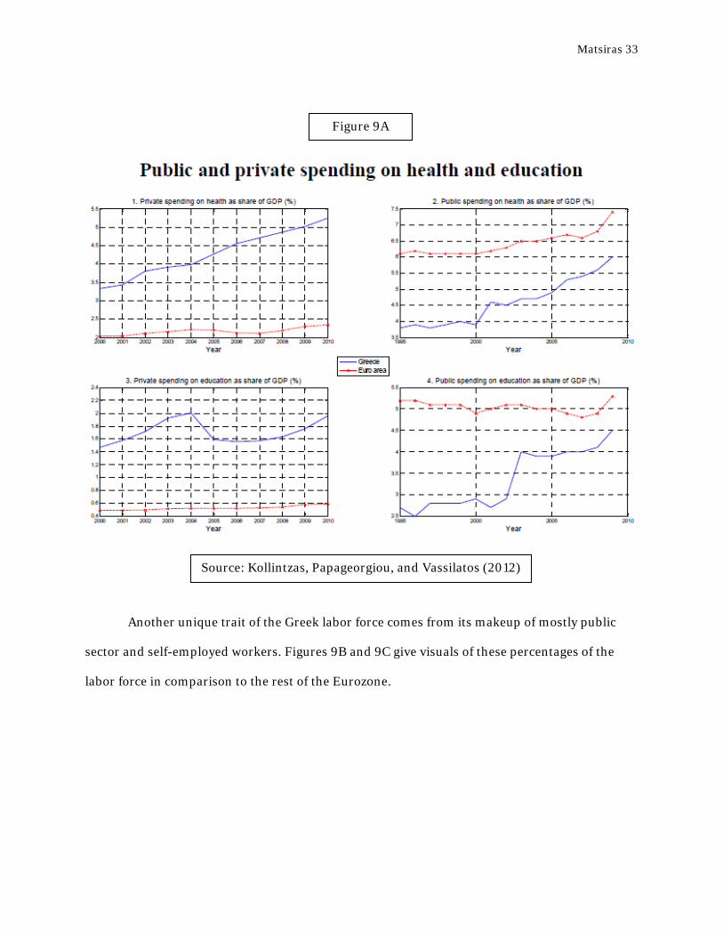
the inefficiency of the Greek labor force. However, as shown in Figure 9A, the Greek public and
private sectors are increasing spending on education, so there is a possibility of resolving the
inadequacies of the labor force in the future.
26 http://www.guardian.co.uk/global-development/2013/jan/30/great-escape-european-migrants-fleeing-recession
Matsiras 33
Another unique trait of the Greek labor force comes from its makeup of mostly public
sector and self-employed workers. Figures 9B and 9C give visuals of these percentages of the
labor force in comparison to the rest of the Eurozone.
Figure 9A
Source: Kollintzas, Papageorgiou, and Vassilatos (2012)

Matsiras 34
Figure 9B
Source: Kollintzas, Papageorgiou, and Vassilatos (2012)
Figure 9C
Source: Kollintzas, Papageorgiou, and Vassilatos (2012)
Matsiras 35
What also becomes evident is the fact that the near majority of the Greek labor force claims to be
self-employed. Although Kollintzas, Papageorgiou, and Vassilatos (2012) claim these workers
choose to identify as self-employed to hide their true income (and thereby bypass higher
taxation), their decision to do so yet again shows the inadequacies of the labor market. Rather
than working in a collective environment or business that could pursue producing more
competitive goods, Greek workers follow economic self-interests to ensure their own financial
stability. It also along these lines that we understand why another large portion of the Greek
labor force is in the public sector, which had (until the recent austerity cuts) much higher job
security and compensation than the private sector. Again, while the public sector is crucial part
of a country’s economy, it is not normally thought of as the most innovative sector in a labor
force. Consequently, the continuing small makeup of the private sector in Greece can be seen as
another reason why Greek exports are not becoming competitive.
iii. Changing Regional Partnerships
While there has been a lot of change in Greece since the implementation of the euro, it is
important to remember that an equal amount of change has occurred in the rest of the Eurozone
(and the rest of the world for that matter). As I found in Section IV Part c, almost every other
Eurozone country has a statistically significant positive euro effect. So, for instance, countries
like Germany and France have increased trade with other partners in the Eurozone and rest of
the world, which have reduced the amount of goods exported from Greece. Consequently, since
joining the Eurozone, Greece has experienced a shift in the location of their top export partners.
To elaborate, in 1996, Greece exported around 60% of their goods to the EU-15 and 12% to
Southeastern Europe.27 This proportion has become 50% and 20%, respectively, in the current
day.
27 Countries considered a part of Southeastern Europe include Albania, Austria, Bosnia and Herzegovina, Bulgaria, Croatia, FYR Macedonia, Greece, Hungary, Italy, Moldova, Montenegro, Romania, Serbia, Slovakia, Slovenia, and Ukraine.

Matsiras 36
Athanasoglou, Backinezos, and Georgiou (2010) credits the shift of trade partners to four
factors: “First, the increasing competition from third countries encountered by Greek exports in
EU-15 markets forced them to find alternative destinations. Second, the already considerable
presence of Greek financial institutions in SE Europe and MME (Mediterranean-Middle
Eastern) countries provided them with the knowledge of the local market environment. Third,
proximity allowed easy access. Finally, these countries were growing fast.” These factors should
make sense intuitively: previous importers of Greek goods can now buy the same, better quality
goods closer to home with another, closer Eurozone trading partner to save money on shipping
expenses. The same is true for Greece, which then restricts trade to an area made up of growing,
but still developing countries in Southeastern Europe and Middle East.
VI. Conclusion
This paper finds that Greece is the Eurozone’s biggest loser in terms of the size of the
euro effect. It also argues that the poor performance of Greek bilateral trade was due to the lack
of competitiveness of Greek exports. Moreover, Greece’s adoption of the euro appears to have
aggravated the decline in the trade with intra-Eurozone and inter-Eurozone partners. While
there is a lot for Greeks to be disappointed in their situation, they must remember that there are
ways to get better. As the Global Competitiveness Report notes, “Greece has a number of
strengths on which it can build, including a reasonably well educated workforce that is adept at
adopting new technologies for productivity enhancements. With the correct growth-enhancing
reforms, there is every reason to believe that Greece will improve its competitiveness in the
coming years.” Athanasoglou, Backinezos, and Georgiou (2010) support this call for reforms,
claiming that “policies that support innovation, variety and quality and create a suitable
environment through investment in research and development are necessary, especially in
sectors where Greece already has a comparative advantage and substantial competitive power.”
And finally, it is also worth noting that Greece is not alone in their struggle. For instance, during

Matsiras 37
the ongoing debt crisis, Germany (among other Eurozone countries) pledged its support in
ensuring Greece’s turnaround to positive growth.28 These growing political ties with neighbors
in Europe, and all other relationships created during the process, will be the invaluable longest
lasting consequences from the adoption of the euro.
28 http://www.bloomberg.com/news/2012-10-05/merkel-to-visit-greece-for-first-time-since-crisis-outbreak.html

Matsiras 38
VII. References
Athanasoglou, P., Backinezos, C. and E. Georgiou, ‘‘Export performance, competitiveness and
commodity composition”, Bank of Greece Working Paper, No. 114, 2010.
Athanasoglou, P. and I. Bardaka, ‘‘Price and non-price competitiveness of exports of
manufactures”, Bank of Greece Working Paper, No. 69, 2010.
Baldwin, R., “The Euro’s Trade Effect”, European Central Bank Working Paper, No. 594, 2006.
Bennett, H., Escolano, J., Fabrizio, S., Gutierrez, E., Ivaschenko, I., Lissovolik, B., Moreno-
Badia, M., Schule, W., Tokarick, S., Xiao, Y., and Z. Zarnic, “Competitiveness in the
Southern Euro Area: France, Greece, Italy, Portugal, and Spain.” IMF Working Paper,
2008.
Flam, H. and H. Nordstrom, “Trade Volume of the Euro: Aggregate and Sector Estimates”,
Institute for International Economics Studies, 2003.
Global Competitiveness Report 2012-2013. World Economic Forum, 2013.
Kollintzas, T., Papageorgiou, D., and V. Vassilatos, “An Explanation of the Greek Crisis: ‘The
Insiders – Outsiders Society,” Centre for Economic Policy Research Discussion Paper
Series, 2012.
Micco, A., Stein, E. and G. Ordoñez, “The Currency Union Effect on Trade: Early Evidence from
the European Union”, Economic Policy, 18(37), 315-356, 2003.
Rose, A. “One Money, One Market: The Effect of Common Currencies on Trade.” Economic
Policy 15.30, 2000: 7-46. Print.
Rose, A. “Is EMU Becoming an Optimum Currency Area? The Evidence on Trade and Business
Cycle Synchronization.” Working Paper, 2008,
http://faculty.haas.berkeley.edu/arose/EMUMetaECB.pdf.
Tinbergen, J., “Shaping the World Economy: Suggestions for an International Economic Policy”,
New York, NY: Twentieth Century Fund, 1962.

Matsiras 39
VIII. Appendix a. Data/Variables
All following data is found for the years 1992-2011. Trade: Exports and imports are measured in terms of millions of US dollars and found on the IMF’s DOTS database. To create the bilateral trade dataset, I download imports and exports from all countries (with every country as its partner). Appending all of these datasets together, I run a simple average all reported imports and exports reported for a specific country pair for a certain year. This average becomes my measure of bilateral trade (referred to as T in the regressions).
There is a minor difference between my dataset of bilateral trade and the ones used in other euro effect papers, which is: most other papers on this topic use the country “Belgium-Luxembourg” to describe trade for both Belgium and Luxembourg.29 Since I could not find any economic indicator data specific to the country “Belgium-Luxembourg,” I replaced any instance that had “Belgium-Luxembourg” as one of the pairs with Belgium (since I have complete data economic indicator data for Belgium), and then exclude Luxembourg from my sample altogether. My reasoning to do so was that Luxembourg is such a small economy that any bilateral trade with them would be negligible to the final analysis. Real GDP/Real GDP per Capita: These are denoted as Y and y, respectively, in the regressions. Real GDP data is taken from the World Bank’s database, World Development Indicators (WDI), using the “GDP (constant 2000 US$)” dataset. I then create a real GDP per capita dataset by dividing real GDP by reported population (“Population, Total”, which can also be found in the WTO’s WDI). Real Effective Exchange Rate (REER):This variable is the index of real exchange rate with base year 2005, calculated as the nominal effective exchange rate (a measure of the value of a currency against a weighted average of several foreign currencies) divided by a price deflator or index of costs. This means that an increase in the REER is an appreciation of the specific country’s currency. Data can be found on the World Bank’s World Development Indicators database, and is listed as “Real effective exchange rate index (2005=100).”
My method of quantifying the value of a currency is different than what appears in Micco, Stein, and Ordonez (2003). In their paper, the authors the ration of real GDP (in US$) to nominal GDP (in US$) as their statistic on real exchange rates because of the following rational:
"Since Real GDP = Nom GDP (in domestic currency) / GDP deflator, and Nominal GDP in dollars = Nominal GDP (in domestic currency) / Nominal exchange rate, the ratio between the two is the nominal exchange rate / GDP deflator, which we use as our index of the real exchange rate. If we multiplied this index by the US GDP deflator we would obtain the bilateral Real Exchange Rate vis-à-vis the US."
One could see their calculation being more focused towards bilateral trade whereas the REER is more multilateral. Consequently, their estimates of the effect of a country’s real exchange rate are always negative, whereas mine are always positive. Regardless of which measure, my estimates of the BothEZ and OneEZ terms only inflate around 1% when I use the real exchange rate rather than REER, so I would feel equally comfortable with using either in my paper. All that will happen is there is an unusual sign on one of the nuisance coefficients.
29 This is likely the result of how trade data was collected, for before 1999, the IMF refers to both Belgium and Luxembourg as the single country, “Belgium-Luxembourg.”

Matsiras 40
Free Trade Agreements (FTAs): This is a dummy variable that indicates whether the trading pair of countries is a part of a free trade agreement. For this I find the data on the World Trade Organization’s database.
It is worth mentioning that most papers site Frankel (1997) as their main source; however, when considering the selected sample of countries in this analysis, this list is essentially made up of 4 different FTAs: the European Free Trade Association (EFTA), the Central European Free Trade Agreement (CEFTA), the North American Free Trade Agreement (NAFTA), and the Australia New Zealand Closer Economic Relations Trade Agreement (ANZCERTA). Besides the fact that this fairly outdated, this list also grossly underestimates the actual number of FTAs during the 1990s and 2000s. That is why I use the WTO statistics database, which lists every FTA (in force and inactive) and to my tally has around 51 FTAs during these two decades during the sample. All told, this could be why my values and significance are somewhat different than previous papers, but by and large the more important results stay constant in significance. EU (European Union): This is the dummy variable that indicates whether a country is in the European Union at a certain time t. EUtrend: Calculated as EU*year. BothEZ: A dummy variable indicating whether the trading partners are both in the Eurozone at time t. OneEZ: A dummy variable indicating whether only one of the trading partners is in the Eurozone at time t. EMU2: A dummy variable indicating whether the trading partners are or will be in the Eurozone. For example, EMU2=1 for Greece-Germany in 1995, even though the euro did not exist. EMU1: A dummy variable indicating whether only one of the trading partners is or will be in the Eurozone. For example, EMU1=1 for Greece-Switzerland in 1995, even though the euro did not exist.

Matsiras 41
b. List of Countries in Samples
Sample Important Dates
MSO Updated MSO
EU Country (Year of Affiliation)
Eurozone (Year Adopted euro)
Australia Australia Austria Austria 1995 1999 Belgium Belgium 1952 1999 Canada Canada Denmark Denmark 1973 Finland Finland 1995 1999 France France 1952 1999 Germany Germany 1952 1999 Greece Greece 1981 2001 Iceland Iceland Ireland Ireland 1973 1999 Italy Italy 1952 1999 Japan Japan New Zealand New Zealand Netherlands Netherlands 1952 1999 Norway Norway Portugal Portugal 1986 1999 Spain Spain 1986 1999 Sweden Sweden 1995 Switzerland Switzerland United Kingdom United Kingdom 1973 United States United States Cyprus 2004 2008 Estonia 2004 2011 Malta 2004 2008 Slovakia 2004 2009 Slovenia 2004 2007

Matsiras 42
c. List of Free Trade Agreements For the end date, “Present” means that the free trade agreement is still active.
FTA Status Start Date
End Date
ASEAN - Australia - New Zealand In Force 2010 Present
ASEAN – India In Force 2010 Present
ASEAN – Japan In Force 2008 Present
ASEAN - Korea, Republic of In Force 2009 Present
ASEAN Free Trade Area (AFTA) In Force 1992 Present
Australia – Chile In Force 2009 Present
Australia - New Zealand (ANZCERTA) In Force 1983 Present
Australia - Papua New Guinea (PATCRA) In Force 1977 Present
Canada – Chile In Force 1997 Present
Canada – Colombia In Force 2011 Present
Canada - Costa Rica In Force 2002 Present
Canada – Israel In Force 1997 Present
Canada – Peru In Force 2009 Present
Canada - US Free Trade Agreement (CUSFTA) Inactive 1989 1994 Central European Free Trade Agreement (CEFTA) Inactive 1993 2004 Central European Free Trade Agreement (CEFTA) - Accession of Slovenia Inactive 1996 2004
Central European Free Trade Agreement (CEFTA) 2006 In Force 2007 Present
China - New Zealand In Force 2008 Present
EC - Czech and Slovak Federal Republic Interim Agreement Inactive 1992 1995 EC - Estonia Agreement Inactive 1995 2004 EC - Finland Agreement Inactive 1974 1994 EC - Greece Additional Protocol Inactive 1975 1981 EC - Poland Europe Agreement Inactive 1994 2004 EC - Poland Interim Agreement of 1991 Inactive 1992 1994 EC - Portugal Agreement of 1972 Inactive 1973 1976 E+A27C - Portugal Interim Agreement Inactive 1976 1986 EC - Slovak Republic Europe Agreement Inactive 1995 2004

Matsiras 43
EC - Slovenia Cooperation Agreement Inactive 1993 1997 EC - Slovenia Interim Agreement Inactive 1997 2004 EC - Spain Agreement of 1970 Inactive 1970 1986 EC - Sweden Agreement Inactive 1973 1995 EFTA - Estonia Free Trade Agreement Inactive 1996 2004 EFTA - Slovak Republic Agreement Inactive 1992 2004 EFTA – Slovenia Inactive 1995 2004 EFTA - Spain Agreement Inactive 1980 1986
EFTA accession of Iceland In Force 1970 Present
Estonia - Norway Free Trade Agreement Inactive 1992 1996 Estonia - Sweden Free Trade Agreement Inactive 1992 1995 Estonia - Switzerland Free Trade Agreement Inactive 1993 1996
EU – Iceland In Force 1973 Present
EU – Norway In Force 1973 Present
EU - Switzerland – Liechtenstein In Force 1973 Present
European Free Trade Association (EFTA) In Force 1960 Present
Finland - Estonia Protocol Inactive 1992 1995 Finland - German Democratic Republic Agreement Inactive 1975 1989 Finland-European Free Trade Association (FINEFTA) Inactive 1961 1986 Ireland - United Kingdom Free Trade Area Inactive 1966 1973
Japan – Switzerland In Force 2009 Present
North American Free Trade Agreement (NAFTA) In Force 1994 Present
Slovak Republic - Slovenia Free Trade Agreement Inactive 1994 1995 Slovenia – Estonia Inactive 1997 2004
Matsiras 44
d. Regression Tables
Table 1A
MSO: 1992-
2002 MSO: 1992-
2011 Updated
MSO VARIABLES Log(T) Log(T) Log(T) BothEZ 0.0961*** 0.129*** 0.107***
(0.0317) (0.0353) (0.0346)
GDP 1.166** 0.701** -0.552
(0.469) (0.318) (0.357)
GDP per Capita -0.0285 0.0827 1.605***
(0.529) (0.362) (0.379)
FTA 0.109*** 0.0859 0.0732
(0.0280) (0.111) (0.105)
EU -2.897 -3.269 6.242
(10.06) (7.475) (7.333)
EUtrend 0.00147 0.00165 -0.00304
(0.00505) (0.00375) (0.00367)
REER Country 1 0.00117* 0.00400*** 0.00746***
(0.000626) (0.000892) (0.000925)
REER Country 2 0.00199*** 0.00411*** 0.00896***
(0.000722) (0.000868) (0.000949)
Constant -40.68*** -18.84* 15.41
(14.68) (10.20) (11.77)
Observations 2,541 4,620 5,400 Country Pair Fixed Effects Yes Yes Yes Time Effect Yes Yes Yes R-squared 0.601 0.788 0.698 Number of Fixed Effects 252 252 324 Robust standard errors in parentheses
*** p<0.01, ** p<0.05, * p<0.1
Matsiras 45
Table 1B
MSO: 1992-
2002 MSO: 1992-
2011 Updated
MSO VARIABLES Log(T) Log(T) Log(T) BothEZ 0.175*** 0.223*** 0.146***
(0.0373) (0.0457) (0.0449)
OneEZ 0.0947*** 0.115*** 0.0442
(0.0250) (0.0365) (0.0310)
GDP 1.525*** 0.822*** -0.540
(0.452) (0.315) (0.359)
GDP per Capita -0.479 -0.0966 1.566***
(0.508) (0.362) (0.385)
FTA 0.120*** 0.114 0.0849
(0.0275) (0.111) (0.104)
EU -1.019 -1.210 7.205
(9.991) (7.578) (7.327)
EUtrend 0.000529 0.000618 -0.00353
(0.00501) (0.00380) (0.00366)
REER Country 1 0.00140** 0.00388*** 0.00751***
(0.000623) (0.000900) (0.000923)
REER Country 2 0.00210*** 0.00411*** 0.00902***
(0.000707) (0.000857) (0.000946)
Constant -50.75*** -21.69** 15.53
(14.20) (10.05) (11.74)
Observations 2,541 4,620 5,400 Country Pair Fixed Effects Yes Yes Yes Time Effect Yes Yes Yes R-squared 0.607 0.791 0.699 Number of Fixed Effects 252 252 324 Robust standard errors in parentheses
*** p<0.01, ** p<0.05, * p<0.1

Matsiras 46
Table 2A
MSO: 1992-
2002 MSO: 1992-
2011 Updated
MSO VARIABLES Log(T) Log(T) Log(T) GDP 1.110** 0.654** -0.576
(0.470) (0.320) (0.358)
GDP per Capita 0.0482 0.161 1.659***
(0.531) (0.365) (0.377)
FTA 0.114*** 0.0904 0.0802
(0.0282) (0.111) (0.105)
EU -2.887 1.024 11.82
(11.24) (8.619) (8.602)
EUtrend 0.00146 -0.000499 -0.00584
(0.00564) (0.00432) (0.00430)
REER Country 1 0.00107* 0.00390*** 0.00732***
(0.000638) (0.000914) (0.000965)
REER Country 2 0.00190*** 0.00400*** 0.00876***
(0.000729) (0.000891) (0.000978)
EMU2-1993 -0.0242 -0.0285
(0.0170) (0.0179)
EMU2-1994 0.0124 0.00381
(0.0231) (0.0245)
EMU2-1995 0.0416 0.0297 0.00225
(0.0293) (0.0319) (0.0285)
EMU2-1996 0.0218 0.0101 -0.00748
(0.0322) (0.0335) (0.0313)
EMU2-1997 -0.0749* -0.0998** -0.0959**
(0.0417) (0.0506) (0.0442)
EMU2-1998 -0.0207 -0.0431 -0.0590
(0.0427) (0.0520) (0.0478)
EMU2-1999 0.0868** 0.0735* 0.0106
(0.0401) (0.0421) (0.0456)
EMU2-2000 0.0602 0.0643 0.0600
(0.0469) (0.0476) (0.0481)
EMU2-2001 0.0798 0.0752 0.111**
(0.0484) (0.0475) (0.0548)
EMU2-2002 0.102* 0.0969* 0.0902
(0.0547) (0.0500) (0.0575)
EMU2-2003
0.154*** 0.0750
(0.0514) (0.0571)
EMU2-2004
0.158*** 0.0718
(0.0551) (0.0600)
EMU2-2005
0.136** 0.0907
(0.0576) (0.0644)
EMU2-2006
0.129** 0.0896
(0.0603) (0.0693)
EMU2-2007
0.146** 0.136*
(0.0638) (0.0720)
EMU2-2008
0.124* 0.0880
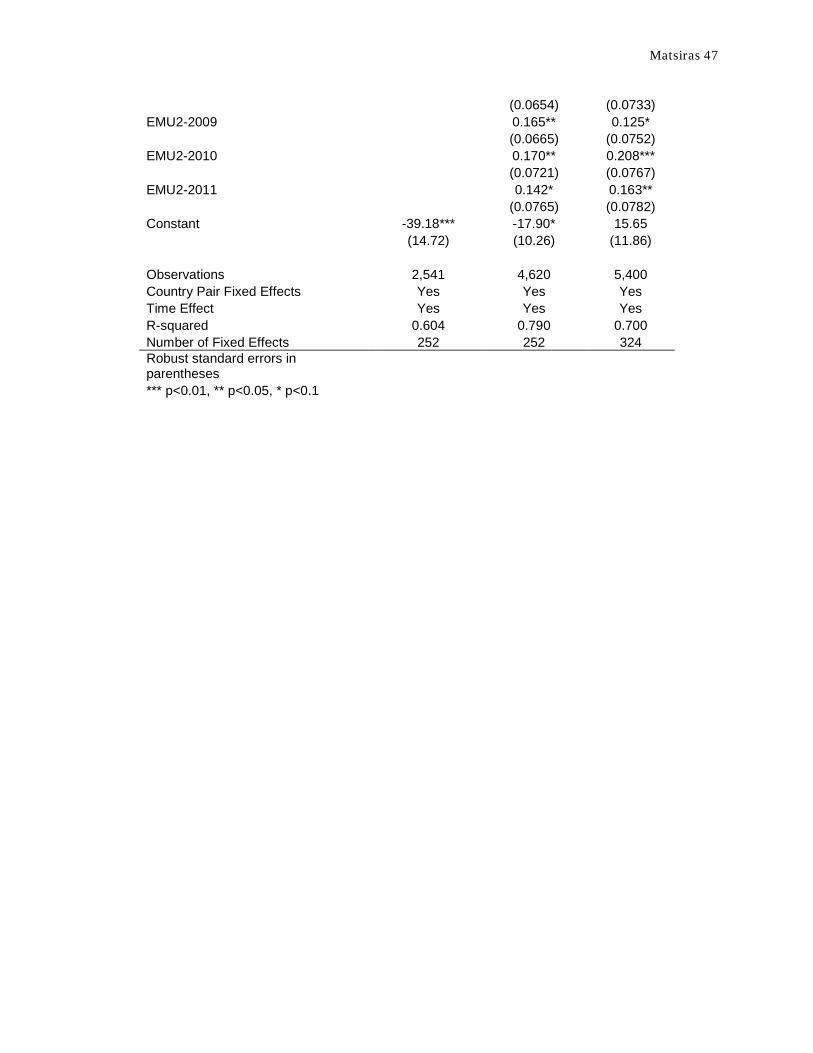
Matsiras 47
(0.0654) (0.0733)
EMU2-2009
0.165** 0.125*
(0.0665) (0.0752)
EMU2-2010
0.170** 0.208***
(0.0721) (0.0767)
EMU2-2011
0.142* 0.163**
(0.0765) (0.0782)
Constant -39.18*** -17.90* 15.65
(14.72) (10.26) (11.86)
Observations 2,541 4,620 5,400 Country Pair Fixed Effects Yes Yes Yes Time Effect Yes Yes Yes R-squared 0.604 0.790 0.700 Number of Fixed Effects 252 252 324 Robust standard errors in parentheses
*** p<0.01, ** p<0.05, * p<0.1

Matsiras 48
Table 2B
MSO:1992-
2002 MSO:1992-
2011 Updated
MSO VARIABLES Log(T) Log(T) Log(T) GDP 1.156** 0.668** -0.560
(0.469) (0.320) (0.356)
GDP per Capita -0.0155 0.139 1.627***
(0.529) (0.365) (0.376)
FTA 0.109*** 0.0896 0.0792
(0.0280) (0.111) (0.106)
EU -2.366 1.049 10.55
(10.34) (8.400) (7.766)
EUtrend 0.00120 -0.000513 -0.00519
(0.00518) (0.00421) (0.00388)
REER Country 1 0.00115* 0.00391*** 0.00738***
(0.000627) (0.000911) (0.000947)
REER Country 2 0.00197*** 0.00400*** 0.00887***
(0.000724) (0.000887) (0.000971)
BothEZ-1999 0.104*** 0.0878*** 0.0754**
(0.0249) (0.0248) (0.0302)
BothEZ-2000 0.0789** 0.0775** 0.0664**
(0.0330) (0.0314) (0.0336)
BothEZ-2001 0.0902** 0.0921*** 0.0228
(0.0360) (0.0333) (0.0341)
BothEZ-2002 0.112** 0.114*** 0.0622*
(0.0442) (0.0387) (0.0377)
BothEZ-2003
0.171*** 0.131***
(0.0382) (0.0365)
BothEZ-2004
0.175*** 0.178***
(0.0433) (0.0382)
BothEZ-2005
0.153*** 0.162***
(0.0465) (0.0396)
BothEZ-2006
0.146*** 0.0984**
(0.0487) (0.0417)
BothEZ-2007
0.163*** 0.118***
(0.0528) (0.0420)
BothEZ-2008
0.141** 0.0709
(0.0552) (0.0523)
BothEZ-2009
0.182*** 0.110**
(0.0574) (0.0532)
BothEZ-2010
0.187*** 0.194***
(0.0630) (0.0571)
BothEZ-2011
0.159** 0.149***
(0.0677) (0.0555)
Constant -40.38*** -18.16* 15.44
(14.67) (10.25) (11.79)
Observations 2,541 4,620 5,400 Country Pair Fixed Effects Yes Yes Yes

Matsiras 49
Time Effects Yes Yes Yes R-squared 0.601 0.789 0.699 Number of Fixed Effects 252 252 324 Robust standard errors in parentheses
*** p<0.01, ** p<0.05, * p<0.1

Matsiras 50
Table 2C
MSO:1992-
2002 MSO:1992-
2011 Updated
MSO VARIABLES Log(T) Log(T) Log(T) GDP 1.519*** 0.767** -0.553
(0.451) (0.320) (0.360)
GDP per Capita -0.471 -0.00709 1.586***
(0.508) (0.366) (0.383)
FTA 0.120*** 0.113 0.0673
(0.0276) (0.112) (0.106)
EU 0.360 5.001 12.13
(10.31) (8.751) (7.938)
EUtrend -0.000162 -0.00249 -0.00598
(0.00517) (0.00439) (0.00397)
REER Country 1 0.00136** 0.00375*** 0.00753***
(0.000625) (0.000935) (0.000963)
REER Country 2 0.00203*** 0.00402*** 0.00905***
(0.000708) (0.000885) (0.000982)
BothEZ-1999 0.163*** 0.128*** 0.0955**
(0.0283) (0.0286) (0.0474)
BothEZ-2000 0.138*** 0.121*** 0.104**
(0.0418) (0.0407) (0.0453)
BothEZ-2001 0.187*** 0.181*** 0.0444
(0.0447) (0.0424) (0.0499)
BothEZ-2002 0.223*** 0.217*** 0.116**
(0.0530) (0.0484) (0.0528)
BothEZ-2003
0.314*** 0.197***
(0.0499) (0.0562)
BothEZ-2004
0.327*** 0.266***
(0.0586) (0.0573)
BothEZ-2005
0.289*** 0.241***
(0.0673) (0.0592)
BothEZ-2006
0.276*** 0.142**
(0.0692) (0.0635)
BothEZ-2007
0.294*** 0.168***
(0.0708) (0.0592)
BothEZ-2008
0.223*** 0.0726
(0.0758) (0.0684)
BothEZ-2009
0.274*** 0.113
(0.0826) (0.0740)
BothEZ-2010
0.288*** 0.226***
(0.0861) (0.0742)
BothEZ-2011
0.271*** 0.195**
(0.0944) (0.0785)
OneEZ-1999 0.0735*** 0.0489** 0.0227
(0.0211) (0.0228) (0.0444)
OneEZ-2000 0.0680** 0.0525 0.0495
(0.0310) (0.0321) (0.0377)
OneEZ-2001 0.115*** 0.112*** 0.0200

Matsiras 51
(0.0323) (0.0322) (0.0456)
OneEZ-2002 0.134*** 0.130*** 0.0702
(0.0344) (0.0347) (0.0430)
OneEZ-2003
0.186*** 0.0903*
(0.0373) (0.0471)
OneEZ-2004
0.197*** 0.126***
(0.0443) (0.0464)
OneEZ-2005
0.172*** 0.111**
(0.0535) (0.0496)
OneEZ-2006
0.160*** 0.0543
(0.0535) (0.0547)
OneEZ-2007
0.158*** 0.0631
(0.0532) (0.0498)
OneEZ-2008
0.0828 -0.0172
(0.0577) (0.0480)
OneEZ-2009
0.0930 -0.0168
(0.0630) (0.0539)
OneEZ-2010
0.105 0.0196
(0.0645) (0.0568)
OneEZ-2011
0.118* 0.0372
(0.0707) (0.0632)
Constant -50.55*** -20.51** 15.85
(14.16) (10.20) (11.85)
Observations 2,541 4,620 5,400 Country Pair Fixed Effects Yes Yes Yes Time Effects Yes Yes Yes R-squared 0.609 0.794 0.701 Number of Fixed Effects 252 252 324 Robust standard errors in parentheses
*** p<0.01, ** p<0.05, * p<0.1
Matsiras 52
Table 3 Part 1 Austria Belgium Cyprus Estonia Finland VARIABLES Log(T) Log(T) Log(T) Log(T) Log(T)
BothEZ*t*X -8.08e-06 0.000257**
* 0.000209**
*
-0.000107*
*
(3.48e-05) (5.51e-05) (7.73e-05)
(4.18e-05)
BothEZ*t*NotX 7.45e-05*** 5.20e-05** 4.58e-05**
7.29e-05***
8.76e-05***
(2.39e-05) (2.27e-05) (2.13e-05) (2.24e-05) (2.34e-05)
OneEZ*t*X 2.99e-05 0.000182**
* 2.86e-05
-4.84e-05
(2.06e-05) (3.13e-05) (4.39e-05)
(4.22e-05)
OneEZ*t*NotX 2.00e-05 1.53e-05 1.93e-05 2.20e-05 2.47e-05
(1.58e-05) (1.56e-05) (1.65e-05) (1.55e-05) (1.56e-05)
GDP -0.533 -0.507 -0.819** -0.540 -0.600*
(0.358) (0.356) (0.347) (0.358) (0.356)
GDP per Capita 1.563*** 1.571*** 1.889*** 1.567*** 1.684***
(0.384) (0.383) (0.359) (0.385) (0.380)
FTA 0.0847 0.0833 0.0998 0.0850 0.0891
(0.104) (0.105) (0.101) (0.104) (0.104)
EU 7.239 7.211 6.814 7.257 8.246
(7.313) (7.193) (7.448) (7.329) (7.345)
EUtrend -0.00354 -0.00353 -0.00335 -0.00355 -0.00405
(0.00366) (0.00360) (0.00372) (0.00366) (0.00367)
REER Country 1 0.00752**
* 0.00745*** 0.00763*** 0.00751**
* 0.00724***
(0.000923) (0.000925) (0.000930)
(0.000923) (0.000900)
REER Country 2 0.00903**
* 0.00896*** 0.00909*** 0.00902**
* 0.00869***
(0.000948) (0.000942) (0.000939)
(0.000946) (0.000946)
Year 0.0251*** 0.0243*** 0.0281*** 0.0253*** 0.0247***
(0.00644) (0.00635) (0.00646) (0.00645) (0.00643)
Constant -34.76*** -34.78*** -32.33*** -34.95*** -32.87***
(6.931) (6.889) (6.809) (6.927) (6.819)
Observations 5,400 5,400 5,400 5,400 5,400 Country Pair Fixed Effects Yes Yes Yes Yes Yes Time Effects Yes Yes Yes Yes Yes R-squared 0.699 0.705 0.702 0.699 0.700 Number of Fixed Effects 324 324 324 324 324 Robust standard errors in parentheses
*** p<0.01, ** p<0.05, * p<0.1

Matsiras 53
Table 3 Part 2 Finland France Germany Greece VARIABLES Log(T) Log(T) Log(T) Log(T)
BothEZ*t*X -
0.000107** -2.06e-05 1.99e-06 -
0.000125***
(4.18e-05) (3.93e-05) (2.79e-05) (3.85e-05)
BothEZ*t*NotX 8.76e-05***
7.65e-05***
7.27e-05*** 9.12e-05***
(2.34e-05) (2.43e-05) (2.40e-05) (2.33e-05)
OneEZ*t*X -4.84e-05 3.83e-05 5.49e-05***
-9.64e-05***
(4.22e-05) (3.19e-05) (2.00e-05) (2.95e-05)
OneEZ*t*NotX 2.47e-05 1.94e-05 1.80e-05 3.24e-05**
(1.56e-05) (1.58e-05) (1.58e-05) (1.58e-05)
GDP -0.600* -0.541 -0.505 -0.606*
(0.356) (0.360) (0.362) (0.357)
GDP per Capita 1.684*** 1.575*** 1.551*** 1.690***
(0.380) (0.390) (0.386) (0.384)
FTA 0.0891 0.0851 0.0833 0.0910
(0.104) (0.104) (0.105) (0.104)
EU 8.246 7.293 7.106 6.840
(7.345) (7.362) (7.289) (7.174)
EUtrend -0.00405 -0.00357 -0.00348 -0.00335
(0.00367) (0.00368) (0.00364) (0.00359)
REER Country 1 0.00724*** 0.00752*** 0.00753*** 0.00749***
(0.000900) (0.000926) (0.000925) (0.000908)
REER Country 2 0.00869*** 0.00902*** 0.00909*** 0.00893***
(0.000946) (0.000947) (0.000945) (0.000933)
Year 0.0247*** 0.0251*** 0.0241*** 0.0243***
(0.00643) (0.00642) (0.00654) (0.00646)
Constant -32.87*** -34.55*** -34.09*** -31.89***
(6.819) (7.030) (6.940) (6.921)
Observations 5,400 5,400 5,400 5,400 Country Pair Fixed Effects Yes Yes Yes Yes Time Effects Yes Yes Yes Yes R-squared 0.700 0.699 0.699 0.702 Number of Fixed Effects 324 324 324 324 Robust standard errors in parentheses
*** p<0.01, ** p<0.05, * p<0.1

Matsiras 54
Table 3 Part 3 Ireland Italy Malta Netherlands VARIABLES Log(T) Log(T) Log(T) Log(T)
BothEZ*t*X -
0.000121** -3.48e-05 4.24e-06 9.23e-05***
(5.03e-05) (3.04e-05) (9.98e-05) (3.35e-05)
BothEZ*t*NotX 8.54e-05***
7.89e-05***
7.24e-05*** 6.00e-05**
(2.40e-05) (2.43e-05) (2.18e-05) (2.38e-05)
OneEZ*t*X -5.18e-05 -2.59e-05 -2.99e-07 0.000100***
(4.86e-05) (2.47e-05) (6.78e-05) (3.66e-05)
OneEZ*t*NotX 2.40e-05 2.47e-05 2.21e-05 1.44e-05
(1.57e-05) (1.58e-05) (1.71e-05) (1.56e-05)
GDP -0.328 -0.560 -0.540 -0.531
(0.380) (0.358) (0.352) (0.356)
GDP per Capita 1.492*** 1.551*** 1.567*** 1.577***
(0.386) (0.385) (0.373) (0.382)
FTA 0.0818 0.0856 0.0852 0.0832
(0.109) (0.104) (0.104) (0.104)
EU 4.487 7.088 7.199 8.088
(7.163) (7.335) (7.390) (7.236)
EUtrend -0.00217 -0.00347 -0.00352 -0.00396
(0.00358) (0.00367) (0.00370) (0.00362)
REER Country 1 0.00709*** 0.00761*** 0.00751*** 0.00755***
(0.000921) (0.000926) (0.000923) (0.000919)
REER Country 2 0.00876*** 0.00916*** 0.00902*** 0.00898***
(0.000932) (0.000953) (0.000949) (0.000939)
Year 0.0182** 0.0266*** 0.0253*** 0.0246***
(0.00711) (0.00654) (0.00649) (0.00639)
Constant -30.19*** -36.24*** -34.91*** -34.12***
(6.719) (7.028) (6.942) (6.882)
Observations 5,400 5,400 5,400 5,400 Country Pair Fixed Effects Yes Yes Yes Yes Time Effects Yes Yes Yes Yes R-squared 0.700 0.699 0.699 0.701 Number of Fixed Effects 324 324 324 324 Robust standard errors in parentheses
*** p<0.01, ** p<0.05, * p<0.1
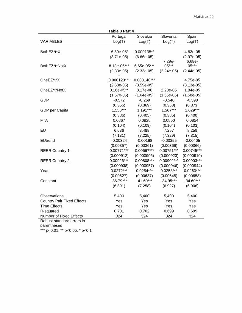
Matsiras 55
Table 3 Part 4 Portugal Slovakia Slovenia Spain VARIABLES Log(T) Log(T) Log(T) Log(T) BothEZ*t*X -6.30e-05* 0.000135**
4.62e-05
(3.71e-05) (6.66e-05)
(2.97e-05)
BothEZ*t*NotX 8.18e-05*** 6.65e-05*** 7.29e-05***
6.68e-05***
(2.33e-05) (2.33e-05) (2.24e-05) (2.44e-05)
OneEZ*t*X -
0.000123*** 0.000140***
4.75e-05
(2.68e-05) (3.59e-05)
(3.13e-05)
OneEZ*t*NotX 3.16e-05** 8.17e-06 2.20e-05 1.84e-05
(1.57e-05) (1.64e-05) (1.55e-05) (1.58e-05)
GDP -0.572 -0.269 -0.540 -0.598
(0.356) (0.369) (0.358) (0.373)
GDP per Capita 1.550*** 1.191*** 1.567*** 1.629***
(0.386) (0.405) (0.385) (0.400)
FTA 0.0867 0.0828 0.0850 0.0854
(0.104) (0.109) (0.104) (0.103)
EU 6.636 3.488 7.257 8.259
(7.131) (7.225) (7.329) (7.315)
EUtrend -0.00324 -0.00168 -0.00355 -0.00405
(0.00357) (0.00361) (0.00366) (0.00366)
REER Country 1 0.00771*** 0.00667*** 0.00751*** 0.00745***
(0.000912) (0.000906) (0.000923) (0.000910)
REER Country 2 0.00926*** 0.00808*** 0.00902*** 0.00903***
(0.000938) (0.000957) (0.000946) (0.000944)
Year 0.0272*** 0.0254*** 0.0253*** 0.0260***
(0.00627) (0.00637) (0.00645) (0.00658)
Constant -36.79*** -41.60*** -34.95*** -34.60***
(6.891) (7.258) (6.927) (6.906)
Observations 5,400 5,400 5,400 5,400 Country Pair Fixed Effects Yes Yes Yes Yes Time Effects Yes Yes Yes Yes R-squared 0.701 0.702 0.699 0.699 Number of Fixed Effects 324 324 324 324 Robust standard errors in parentheses
*** p<0.01, ** p<0.05, * p<0.1
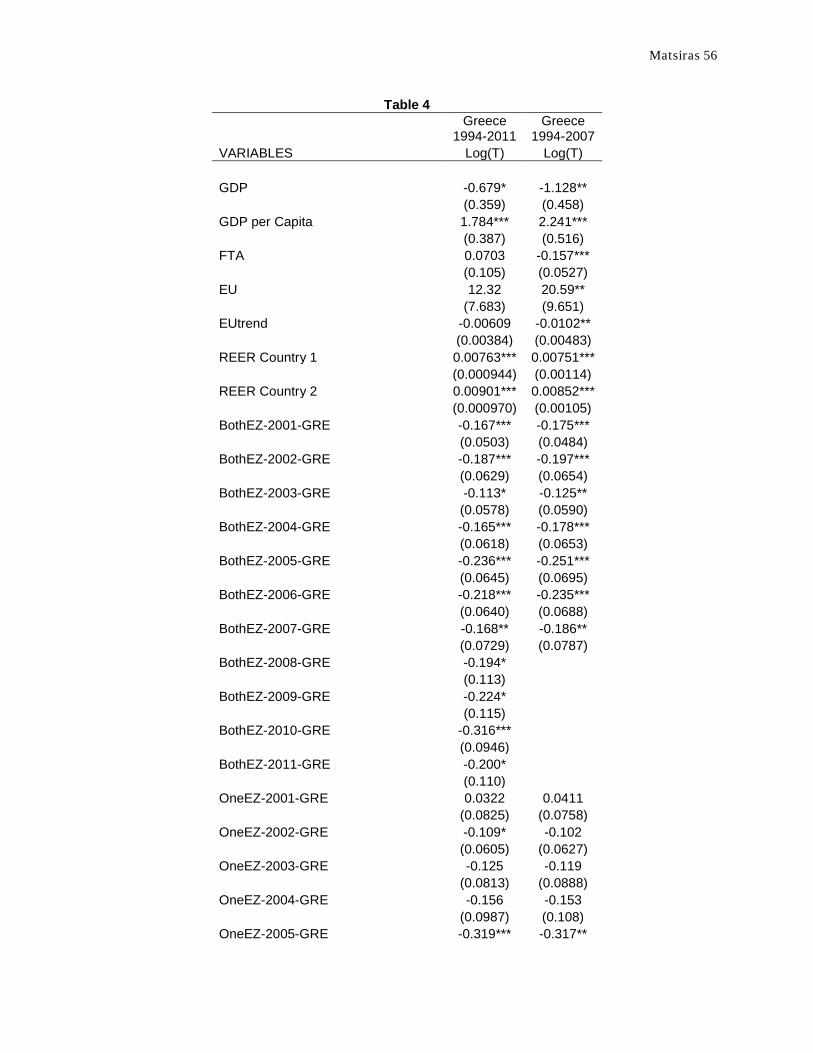
Matsiras 56
Table 4
Greece
1994-2011 Greece
1994-2007 VARIABLES Log(T) Log(T) GDP -0.679* -1.128**
(0.359) (0.458)
GDP per Capita 1.784*** 2.241***
(0.387) (0.516)
FTA 0.0703 -0.157***
(0.105) (0.0527)
EU 12.32 20.59**
(7.683) (9.651)
EUtrend -0.00609 -0.0102**
(0.00384) (0.00483)
REER Country 1 0.00763*** 0.00751***
(0.000944) (0.00114)
REER Country 2 0.00901*** 0.00852***
(0.000970) (0.00105)
BothEZ-2001-GRE -0.167*** -0.175***
(0.0503) (0.0484)
BothEZ-2002-GRE -0.187*** -0.197***
(0.0629) (0.0654)
BothEZ-2003-GRE -0.113* -0.125**
(0.0578) (0.0590)
BothEZ-2004-GRE -0.165*** -0.178***
(0.0618) (0.0653)
BothEZ-2005-GRE -0.236*** -0.251***
(0.0645) (0.0695)
BothEZ-2006-GRE -0.218*** -0.235***
(0.0640) (0.0688)
BothEZ-2007-GRE -0.168** -0.186**
(0.0729) (0.0787)
BothEZ-2008-GRE -0.194*
(0.113)
BothEZ-2009-GRE -0.224*
(0.115)
BothEZ-2010-GRE -0.316***
(0.0946)
BothEZ-2011-GRE -0.200*
(0.110)
OneEZ-2001-GRE 0.0322 0.0411
(0.0825) (0.0758)
OneEZ-2002-GRE -0.109* -0.102
(0.0605) (0.0627)
OneEZ-2003-GRE -0.125 -0.119
(0.0813) (0.0888)
OneEZ-2004-GRE -0.156 -0.153
(0.0987) (0.108)
OneEZ-2005-GRE -0.319*** -0.317**
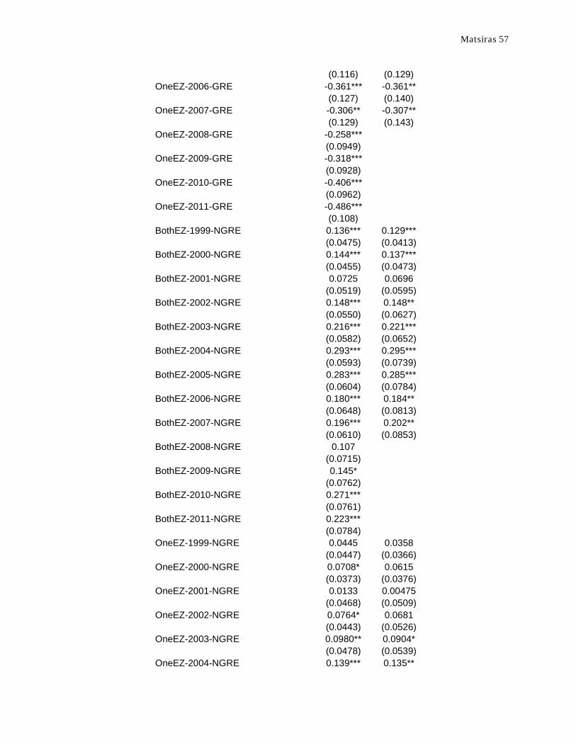
Matsiras 57
(0.116) (0.129)
OneEZ-2006-GRE -0.361*** -0.361**
(0.127) (0.140)
OneEZ-2007-GRE -0.306** -0.307**
(0.129) (0.143)
OneEZ-2008-GRE -0.258***
(0.0949)
OneEZ-2009-GRE -0.318***
(0.0928)
OneEZ-2010-GRE -0.406***
(0.0962)
OneEZ-2011-GRE -0.486***
(0.108)
BothEZ-1999-NGRE 0.136*** 0.129***
(0.0475) (0.0413)
BothEZ-2000-NGRE 0.144*** 0.137***
(0.0455) (0.0473)
BothEZ-2001-NGRE 0.0725 0.0696
(0.0519) (0.0595)
BothEZ-2002-NGRE 0.148*** 0.148**
(0.0550) (0.0627)
BothEZ-2003-NGRE 0.216*** 0.221***
(0.0582) (0.0652)
BothEZ-2004-NGRE 0.293*** 0.295***
(0.0593) (0.0739)
BothEZ-2005-NGRE 0.283*** 0.285***
(0.0604) (0.0784)
BothEZ-2006-NGRE 0.180*** 0.184**
(0.0648) (0.0813)
BothEZ-2007-NGRE 0.196*** 0.202**
(0.0610) (0.0853)
BothEZ-2008-NGRE 0.107
(0.0715)
BothEZ-2009-NGRE 0.145*
(0.0762)
BothEZ-2010-NGRE 0.271***
(0.0761)
BothEZ-2011-NGRE 0.223***
(0.0784)
OneEZ-1999-NGRE 0.0445 0.0358
(0.0447) (0.0366)
OneEZ-2000-NGRE 0.0708* 0.0615
(0.0373) (0.0376)
OneEZ-2001-NGRE 0.0133 0.00475
(0.0468) (0.0509)
OneEZ-2002-NGRE 0.0764* 0.0681
(0.0443) (0.0526)
OneEZ-2003-NGRE 0.0980** 0.0904*
(0.0478) (0.0539)
OneEZ-2004-NGRE 0.139*** 0.135**

Matsiras 58
(0.0461) (0.0602)
OneEZ-2005-NGRE 0.139*** 0.133**
(0.0491) (0.0638)
OneEZ-2006-NGRE 0.0857 0.0804
(0.0543) (0.0669)
OneEZ-2007-NGRE 0.0892* 0.0836
(0.0496) (0.0669)
OneEZ-2008-NGRE 0.00355
(0.0486)
OneEZ-2009-NGRE 0.00388
(0.0552)
OneEZ-2010-NGRE 0.0467
(0.0582)
OneEZ-2011-NGRE 0.0696
(0.0641)
Constant 18.50 33.10**
(11.85) (14.35)
Observations 5,400 4,200 Country Pair Fixed Effects Yes
Time Effects Yes Number of Fixed Effects 324 324
R-squared 0.707 0.658 Robust standard errors in parentheses
*** p<0.01, ** p<0.05, * p<0.1