The Great Andromeda Galaxy Princeton, 19 June 2012 · The Great Andromeda Galaxy Princeton, 19 June...
70
M31: black hole & dynamics of nucleus John Magorrian The Great Andromeda Galaxy Princeton, 19 June 2012
-
Upload
phungnguyet -
Category
Documents
-
view
216 -
download
0
Transcript of The Great Andromeda Galaxy Princeton, 19 June 2012 · The Great Andromeda Galaxy Princeton, 19 June...

M31: black hole & dynamics of nucleus
John Magorrian
The Great Andromeda GalaxyPrinceton, 19 June 2012

1. The black hole at the centre of M31
(just P3)

Photometry of P3(Bender et al 2005)
Distinct component in UV
Scale: P1-P2 separated by ∼ 0.5” ∼ 2 pc.

Photometry of P3(Bender et al 2005)
Distinct component in UV
Scale: P1-P2 separated by ∼ 0.5” ∼ 2 pc.

Properties of P3(Bender et al 2005, Lauer et al 2012)
Distinct from surrounding P1–P2 eccentric disc:100’s of A stars100-200 Myr old∼ exponential profile, r0 ' 0.1” (0.4 pc)possible change for r < 0.03”.
STIS spectra 350-500 nm includes Ca II H and K, Balmer lines.

Kinematics of P3: razor-thin disc models(Bender et al 2005)
P3 kinematics describedwell by simpleexponential disc model,i = 55,M• ' 1.4× 10⁸ M.

Kinematics of P3: fat Schwarzschild models(Bender et al 2005)
Best-fit model: thin disc around M• = 1.4× 10⁸ M.1-σ range of thick-disc models is (1.1− 2.3)× 108 M.

Kinematics of P3: fat Schwarzschild models(Bender et al 2005)
Best-fit model: thin disc around M• = 1.4× 10⁸ M.1-σ range of thick-disc models is (1.1− 2.3)× 108 M.

2. The eccentric disc around the BH
(What’s happening outside P3?)
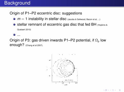
Background
Origin of P1–P2 eccentric disc: suggestionsm = 1 instability in stellar disc (Jacobs & Sellwood, Bacon et al, ...)
stellar remnant of eccentric gas disc that fed BH (Hopkins &
Quataert 2010)
...Origin of P3: gas driven inwards P1–P2 potential, if Ωp lowenough? (Chang et al 2007).

Background
Origin of P1–P2 eccentric disc: suggestionsm = 1 instability in stellar disc (Jacobs & Sellwood, Bacon et al, ...)
stellar remnant of eccentric gas disc that fed BH (Hopkins &
Quataert 2010)
...Origin of P3: gas driven inwards P1–P2 potential, if Ωp lowenough? (Chang et al 2007).
Motivation“The laws of physics are perfect, but the human brain is not.”
What constraints can we hope to extract from observations?3d shape, orientationinternal orbit structuremeasurement of M• (indep of P3).

Data
WFPC photometry (Lauer et al 98):

Data
WFPC photometry (Lauer et al 98):
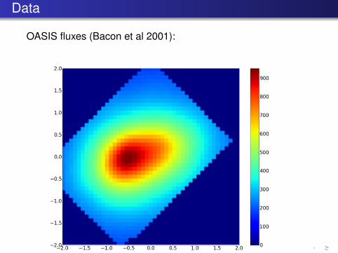
Data
OASIS fluxes (Bacon et al 2001):
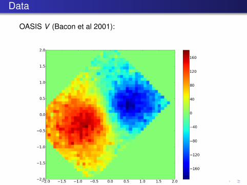
Data
OASIS V (Bacon et al 2001):

Data
OASIS σ (Bacon et al 2001):
Data
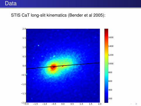
STIS CaT long-slit kinematics (Bender et al 2005):

Data
STIS CaT long-slit kinematics (Bender et al 2005):

Data
More kinematics from, e.g.,van der Marel et al. (1994) (long slit)Kormendy & Bender (1999) (long slit, maj)Statler+99 (1999) (FOC)

2a. Three-dimensional, massless discs

3d models with massless discsPeiris & Tremaine 2003
Purely Keplerian potential: DF f (a,e, I, ω,Ω).Assume disc has biaxial (y , z) symmetry.
Clump of orbits around a = 1, e = 0.7 projected along z:

3d models with massless discsPeiris & Tremaine 2003
Purely Keplerian potential: DF f (a,e, I, ω,Ω).Assume disc has biaxial (y , z) symmetry.
Clump of orbits around a = 1, e = 0.7 projected along y :

3d models with massless discsPeiris & Tremaine 2003
Purely Keplerian potential: DF f (a,e, I, ω,Ω).Assume disc has biaxial (y , z) symmetry.
Clump of orbits around a = 1, e = 0.7 projected along los:
Eulerangles:θl , θi , θa

3d models with massless discs(Peiris & Tremaine 2003)
Peiris & Tremaine (2003) took
f (a,e, I) = g(a) e exp[− [e− em(a)]2
2σe(a)2
]sin I exp
[− I2
2σI(a)2
].
Free parameters:
3 g(a) radial sb profile+2 σI(a) thickness profile+5 em(a), σe eccentricity distn.+1 M•+3 (θl , θi , θa) viewing angle
=14 (neglecting centre)
Fit: WFPC V -band photometry and KB99 (V , σ) long slit.Predict: KB99 LOSVD shapes; STIS, OASIS kinematics.

3d models with massless discs(Peiris & Tremaine 2003)
Some details:For disc thickness:
σI = σ0I exp(−a/aI).
For em(a), something of the form:
Motivation: encourage round P2, brighter than P1, with dipinbetween P1 and P2.

3d models with massless discs(Peiris & Tremaine 2003: results)
Models with i = 55 (right) are better fits than models alignedwith the large-scale disc (i = 77, left).

3d models with massless discs(Peiris & Tremaine 2003: results)
Models with i = 55 (right) are better fits than models alignedwith the large-scale disc (i = 77, left).

3d models with massless discs(Peiris & Tremaine 2003: results)
Models with i = 55 (right) are better fits than models alignedwith the large-scale disc (i = 77, left).

3d models with massless discs(Peiris & Tremaine 2003: results)
Models with i = 55 (right) are better fits than models alignedwith the large-scale disc (i = 77, left).

3d models with massless discs(Peiris & Tremaine 2003: results)
PT03 models predict the STIS kinematics pretty well(left: aligned, right: unaligned):

3d models with massless discs(Peiris & Tremaine 2003: results)
PT03 models predict the STIS kinematics pretty well(left: aligned, right: unaligned):

3d models with massless discs(Peiris & Tremaine 2003: results)
PT03 models predict the STIS kinematics pretty well(left: aligned, right: unaligned):

3d models with massless discsmultiblob expansion
Peiris & Tremaine (2003) had
f = g(a) e exp[− [e− em(a)]2
2σe(a)2
]sin I exp
[− I2
2σI(a)2
].
To avoid need to think about em(a), try instead
f =∑
i
wi exp[−(a− ai)
2
2σ2a
]e exp
[−(e− ei)
2
2σ2e
]sin I exp
[− I2
2σI,i2
].
Multiblob expansion
Blobs centred on fixed pts in (a,e) plane, plusσI,i = 15, 30, 45.
Free parameters:30× 9× 3 (na × ne × ni ) blob weights;
×2 if counter-rotating orbits included;M•;orientation of disc on sky (θl , θi , θa).
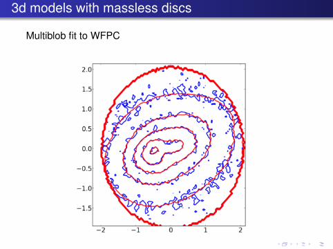
3d models with massless discs
Multiblob fit to WFPC
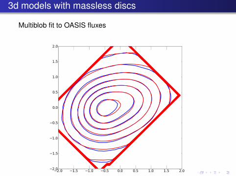
3d models with massless discs
Multiblob fit to OASIS fluxes
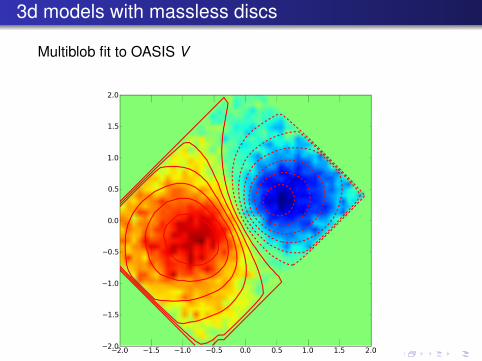
3d models with massless discs
Multiblob fit to OASIS V

3d models with massless discs
Multiblob fit to OASIS σ

3d models with massless discs
Multiblob fit to “STIS fluxes”
3d models with massless discs
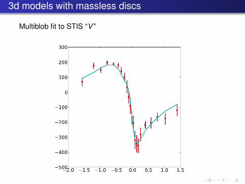
Multiblob fit to STIS “V ”

3d models with massless discs
Multiblob fit to STIS “σ”

Why is the fit to σ so poor?
V and σ measured by fitting Gaussian model LOSVDs tospectra...
...my models assume V and σ are 1st and 2nd moments.
(not all LOSVDs agree this well...)

3d models with massless discsmultiblob expansion results
What does the disc look like? LOS projection:

3d models with massless discsmultiblob expansion results
What does the disc look like? Edge-on:
3d models with massless discsmultiblob expansion results
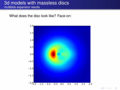
What does the disc look like? Face-on:

3d models with massless discsmultiblob expansion results
What does the disc look like? Face-on:

3d models with massless discsmultiblob expansion results
What does the disc look like? Face-on:

3d models with massless discsmultiblob expansion results
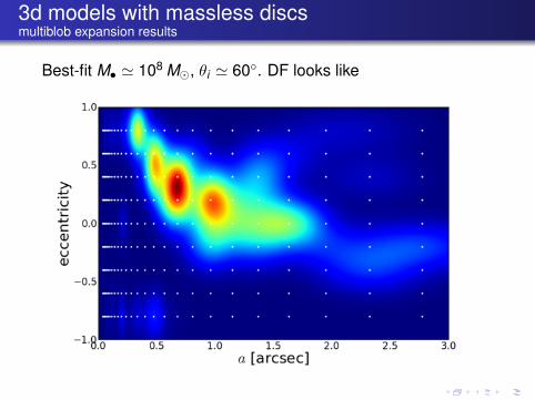
Best-fit M• ' 108 M, θi ' 60. DF looks like
3d models with massless discsmultiblob expansion results
Best-fit M• ' 108 M, θi ' 60. DF looks like

3d models with massless discsmultiblob expansion results
Dispersion of I and e as function of a:

3d models with massless discsmultiblob expansion results
Dispersion of I and e as function of a:

3d models with massless discsmultiblob expansion results
Dispersion of I and e as function of a: NB: σI 6' 0.5σe!

3d models with massless discs
Summary of 3d models to date
Eitherprovide only moderately good fit to photometry (PT03), orbarely fit kinematics (me)
Don’t make use of LOSVD informationCavalier treatment of errorszzz
Neglect the mass of the disc (∼ 0.1M•)!
Three (semi-)independent implementations. All findM• = 108M to approximately 10%.
Degeneracies in fit: which (a,e) features are essential?Dynamically informed prior on (a,e, I) might be good.

2b. Two-dimensional, massive discs
Massive 2d discs: overview
T95: Massive disc makes orbits precess at different rates.Coherent eccentric disc won’t last long.
Assume BH-plus-disc system stationary in frame rotating atpattern speed Ωp.
Sridhar & Touma (1999): in nearly Keplerian potential,almost all orbits regularfamily of loop orbits that reinforce l = 1 perturbations
Problem (2d)
What are M•, ΩP and ρdisc(x , y) for M31?

Weak 2d discs(Statler 1999; Salow & Statler 2001, 2004)
SS04 assume DF
f (a,e, ω) = g(a) exp[− [e − e0(a)]2
2σ2e
]exp
[− ω2
2σ2ω
].
Iterative scheme for finding ρ(x , y) given M•, Ω. E.g.,
Adjust free parameters to match photometry (along P1–P2only) and kinematics.

Weak 2d discs(Statler 1999; Salow & Statler 2001, 2004)
Best-fitting self-gravitating models in literature:

Schwarzschild’s method!(Sambhus & Sridhar 2002, TdZ talk later)
For 2d disc, we “know” ρ(x , y) from photometry:
Find combination of orbits thatself-consistently reproducesthis ρ(x , y) (with someassumed M•, Ωp).
Schwarzschild (1982): triaxial ρ(x , y , z) plus known Ωp.Present problem: ρ(x , y), unknown M•, Ωp,
obs errors

Schwarzschild’s method!(Sambhus & Sridhar 2002)
Samples from orbit library, plus fit to photometry:
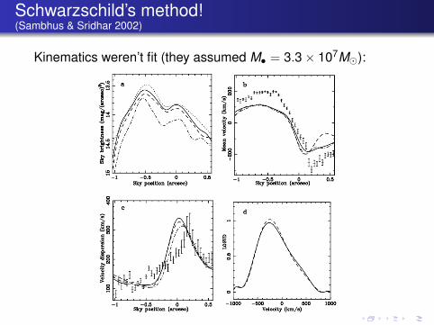
Schwarzschild’s method!(Sambhus & Sridhar 2002)
Kinematics weren’t fit (they assumed M• = 3.3× 10⁷M):

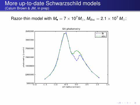
More up-to-date Schwarzschild models(Calum Brown & JM, in prep)
Razor-thin model with M• = 7× 10⁷M, Mdisc = 2.1× 10⁷ M:

More up-to-date Schwarzschild models(Calum Brown & JM, in prep)
Razor-thin model with M• = 7× 10⁷M, Mdisc = 2.1× 10⁷ M:
More up-to-date Schwarzschild models(Calum Brown & JM, in prep)
Razor-thin model with M• = 7× 10⁷M, Mdisc = 2.1× 10⁷ M:

More up-to-date Schwarzschild models(Calum Brown & JM, in prep)
Razor-thin model with M• = 7× 10⁷M, Mdisc = 2.1× 10⁷ M:

More up-to-date Schwarzschild models(Calum Brown & JM, in prep)
Razor-thin model with M• = 7× 10⁷M, Mdisc = 2.1× 10⁷ M:

More up-to-date Schwarzschild models(Calum Brown & JM, in prep)
Constraints on pattern speed:
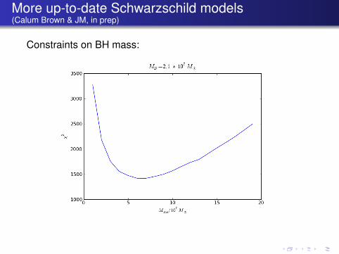
More up-to-date Schwarzschild models(Calum Brown & JM, in prep)
Constraints on BH mass:
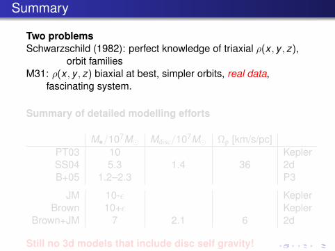
Summary
Two problemsSchwarzschild (1982): perfect knowledge of triaxial ρ(x , y , z),
orbit familiesM31: ρ(x , y , z) biaxial at best, simpler orbits, real data,
fascinating system.
Summary of detailed modelling efforts
M•/107M Mdisc/107M Ωp [km/s/pc]PT03 10 KeplerSS04 5.3 1.4 36 2dB+05 1.2–2.3 P3
JM 10-ε KeplerBrown 10+ε Kepler
Brown+JM 7 2.1 6 2d
Still no 3d models that include disc self gravity!

1 Black hole mass
2 Disk modelsData3d models with massless discs2d massive discs
3 summary