Table of Contents

1. Systems with Variable Particle Numbers

2. Review of the Ensembles

2.1. Microcanonical Ensemble

2.2. Canonical Ensemble

2.3. Grand Canonical Ensemble

3. Average Values on the Grand Canonical Ensemble

3.1. Average Number of Particles in a System

4. The Grand Canonical Ensemble and Thermodynamics

5. Legendre Transforms

5.1. Legendre Transforms for two variables

5.2. Helmholtz Free Energy as a Legendre Transform

6. Legendre Transforms and the Grand Canonical Ensem-

ble

7. Solving Problems on the Grand Canonical Ensemble

Section 1: Systems with Variable Particle Numbers 3

1. Systems with Variable Particle Numbers

We have developed an expression for the partition function of an idealgas.

Toc JJ II J I Back J Doc Doc I

Section 2: Review of the Ensembles 4

2. Review of the Ensembles

2.1. Microcanonical Ensemble

The system is isolated. This is the first bridge or route betweenmechanics and thermodynamics, it is called the adiabatic bridge.

E, V,N are fixed S = k lnΩ(E, V,N)



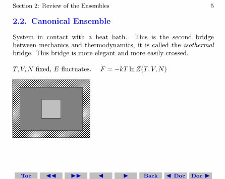
2.2. Canonical Ensemble

System in contact with a heat bath. This is the second bridgebetween mechanics and thermodynamics, it is called the isothermal

bridge. This bridge is more elegant and more easily crossed.

T, V,N fixed, E fluctuates. F = −kT lnZ(T, V,N)



2.3. Grand Canonical Ensemble

System in contact with heat bath/paricle reservoir. This thirdbridge is called the open bridge. T, V, µ fixed, E and N fluctuate.Ω = −kT ln Ξ = −kT lnZ, where Ω is the grand potential andΞ(= Z), is the grand partition function.


Section 3: Average Values on the Grand Canonical Ensemble 7

3. Average Values on the Grand Canonical

Ensemble

For systems in thermal and diffusive contact with a reservoir, letx(N, r) be the value of x when the system has N particles and isin state Nr. The thermal average is thus

〈x〉 =∑

N,r

x(N, r)pNr =

∑

N,r

x(N, r)eβ(Nµ−ENr)

Z

3.1. Average Number of Particles in a System

〈N〉 =

∑

N,r

Neβ(Nµ−ENr)

Z



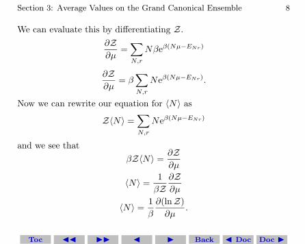
We can evaluate this by differentiating Z.

∂Z

∂µ=∑

N,r

Nβeβ(Nµ−ENr)

∂Z

∂µ= β

∑

N,r

Neβ(Nµ−ENr).

Now we can rewrite our equation for 〈N〉 as

Z〈N〉 =∑

N,r

Neβ(Nµ−ENr)

and we see that

βZ〈N〉 =∂Z

∂µ

〈N〉 =1

βZ

∂Z

∂µ

〈N〉 =1

β

∂(lnZ)

∂µ.



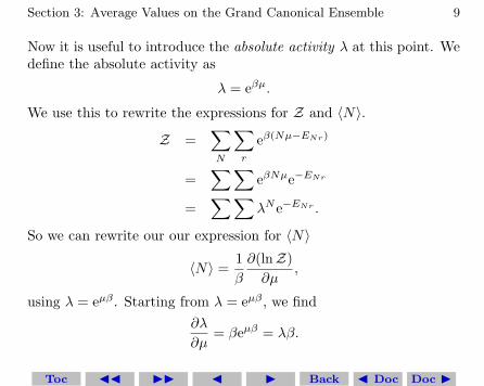
Now it is useful to introduce the absolute activity λ at this point. Wedefine the absolute activity as

λ = eβµ.

We use this to rewrite the expressions for Z and 〈N〉.

Z =∑

N

∑

r

eβ(Nµ−ENr)

=∑∑

eβNµe−ENr

=∑∑

λNe−ENr .

So we can rewrite our our expression for 〈N〉

〈N〉 =1

β

∂(lnZ)

∂µ,

using λ = eµβ . Starting from λ = eµβ , we find

∂λ

∂µ= βeµβ = λβ.



So1

β

∂(lnZ)

∂µ=

1

β

∂(lnZ)

∂λ

∂λ

∂µ=λβ

β

∂(lnZ)

∂λ= λ

∂(lnZ)

∂λ

This is a result of practical importance. We can find λ by matching〈N〉 to N the actual number of particles in the system.

In chemistry, it is common to introduce the fugacity at this point.The definition is close to the definition of the absolute activity, wedefine the fugacity f as

f = eµk .

We will not make further use of the fugacity.In calculating the thermal properties of systems, the ensemble on

which we choose to make the calculations is a matter of convenience.We choose the ensemble independently of the actual environment.This is possible because fluctuations tend to be small. Since N =const is mathematically awkward, the grand ensemble is often themost convenient approach.


Section 4: The Grand Canonical Ensemble and Thermodynamics 11

4. The Grand Canonical Ensemble and Ther-

modynamics

Starting from

Z =∑

N,r

eβ(Nµ−ENr)

and

pNr =eβ(Nµ−ENr)

Z,

we relate the grand canonical ensemble to thermodynamics using theGibbs entropy formula

S = −k∑

r

pr ln pr.

In this case we write the Gibbs entropy formula as

S = −k∑

N,r

pNr ln pNr.


Section 4: The Grand Canonical Ensemble and Thermodynamics 12

Inserting the Gibbs distribution, we get

S = −k∑

N,r

pNr ln

(

eβ(Nµ−ENr)

Z

)

= −k∑

N,r

pNr ln

(

ln

(

1

Z

)

+ βNµ− βENr

)

= −k∑

N,r

pNr ln1

Z− k

∑

N,r

pNrβNµ+ k∑

N,r

pNrβENr

= −k ln1

Z

∑

N,r

pNr − kβµ∑

N,r

pNrN + kβ∑

N,r

ENrpNr

S = k lnZ − kβµ〈N〉+ kβ〈E〉.

And, after rearranging

lnZ =S

k+ βµ〈N〉 − β〈E〉,


Section 5: Legendre Transforms 13

which will normally be written as

lnZ =S

k+ βµN − βE,

where, as usual, we have written E = 〈E〉 and N = 〈N〉.This expression can be further simplified. To simplify it we will

make use of the Legendre transform.

5. Legendre Transforms

Legendre transforms are widely used in mechanics and thermodynam-ics. Legendre transforms transform are most easily explained in onedimension. For each function f(x) define a new function Lf(z), theLegendre transform, as follows:Define

z =df

dx



thus relating the new variable z to the old variable x. We require that

d2f

dx26= 0

to guarantee that we can find the inverse function x(z). Hence wehave a unique relation between x and z. The Legendre transform canbe written as

Lf(z) = zx(z)− f (x(z))

So we simultaneously change our variable to the derivative and modifythe function. Note that in physics the transform is often defined as thenegative of the function above (e.g. F = E − TS) The mathematicaldefinition of the transform is “better” as there is no minus sign in theinverse transformation. But in thermodynamics we want to keep themeaning of the transformed function in terms of energy, and TS −Ewould be awkward. Thus we have seen Legendre transforms but havenot defined them.

That completes the theory as I’ll present it, if you are interestedyou can easily find the complete theory worked out (usually in terms



of mappings) and explicit calculations of the inverse transform. I’mgoing to show you how to figure it out practically for two variables.

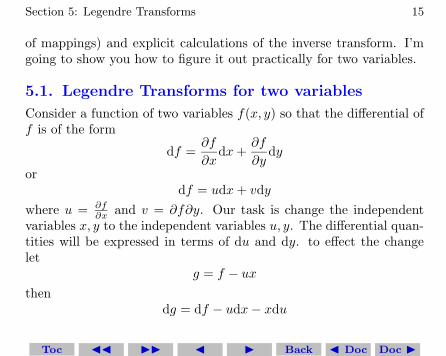
5.1. Legendre Transforms for two variables

Consider a function of two variables f(x, y) so that the differential off is of the form

df =∂f

∂xdx+

∂f

∂ydy

ordf = udx+ vdy

where u = ∂f∂x

and v = ∂f∂y. Our task is change the independentvariables x, y to the independent variables u, y. The differential quan-tities will be expressed in terms of du and dy. to effect the changelet

g = f − ux

thendg = df − udx− xdu



butdf = udx+ vdy

sodg = vdy − xdu.

This is the form we desire. The quantities x and v are now functionsof u and y and are given by

x = −∂g

∂uand v =

∂g

∂y.

In this case, these are our inverse transforms. The transformation ofthe Lagrangian of mechanics to the Hamiltonian is an example of sucha transformation.1

1See for example: Herbert Goldstein, Classical Mechanics, Addison-Wesley,

1950, Chapter 7



5.2. Helmholtz Free Energy as a Legendre Trans-

form

We want to transform from E(S, V,N) to F (T, V,N so using

Lf(z) = f (x(z))− zx(z)

we know T =(

∂E∂S

)

V,Nso we write

LE(N,V, T ) = E(N,V, S(T ))∂E

∂SS

orF = E − TS.

calculating the differential shows that we have changed the indepen-dent variable from S to T .


Section 6: Legendre Transforms and the Grand Canonical Ensemble 18

6. Legendre Transforms and the Grand Canon-

ical Ensemble

Recall we have found

lnZ =S

k+ βµN − βE

we can rewrite this as

−kT lnZ = E − TS − µN.

Rewriting this as−kT lnZ = F − µN

we recognize this as another Legendre transform, as we know thatµ is the conjugate variable of N . Thus we are transforming to aquantity that is a function of µ rather than being a function of N .Such potentials are called grand potentials. This one happens to bethe most useful. So defining

Ω(T, V, µ) = F (T, V,N(µ))−∂F

∂NN


Section 6: Legendre Transforms and the Grand Canonical Ensemble 19

we have

dΩ = dF − µdN −Ndµ = SdT − pdV −Ndµ

The grand potential is the available energy for a system in contactwith a reservoir that provides the energy necessary to keep the systemat constant temperature and the particles necessary to keep it atconstant chemical potential.

We can now relate Ω andZ by writing

Ω = −kT lnZ.

This result is the open bridge between thermodynamics and statisti-cal mechanics. This equation will form the basis of our strategy forderiving thermodynamics from the grand canonical ensemble.

Since we have used the methods before, I am going to summarizethe strategy as you will appreciate the terminology. You wouldn’thave before we had studied the canonical ensemble.


Section 7: Solving Problems on the Grand Canonical Ensemble 20

7. Solving Problems on the Grand Canon-

ical Ensemble

1. Find Z as a function of T, V, µ. (Other mechanical extensivevariables could replace V .

2. Find the grand potential from Ω = −kT lnZ.

3. Find the entropy of the system from

S = −

(

∂Ω

∂T

)

V,µ

and the number of particles from

N = 〈N〉 = −

(

∂Ω

∂µ

)

V,T

4. Use

p = −

(

∂Ω

∂V

)

µ,T


Section 7: Solving Problems on the Grand Canonical Ensemble 21

to find the equation of state.

5. Find any useful thermodynamic potential from

F = Ω+ µN

E = F + TS = Ω+ µN + TS

G = E + pV − TS = F + pV

H = E + pV

6. Study the system using thermodynamics.


The Grand Canonical Ensemble - Faculty Sites at the...

Documents

Transcript of The Grand Canonical Ensemble - Faculty Sites at the...