Steven Goodman

GOES-R Program Senior (Chief) Scientist

NOAA/NESDIS/ GOES-R Program Office

http://www.goes-r.gov

Joint Center for Satellite Data Assimilation SeminarWorld Weather Building, Camp Springs, MD

May 26, 2010

The GOES-R Geostationary Lightning Mapper(GLM) and Opportunities for Assimilation of

the Data into NWP models

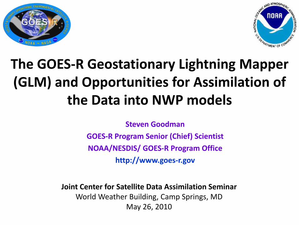
Outline of Presentation

2

1. GLM Instrument2. Physical Basis- Electrification and Lightning3. Lightning Data Assimilation and NWP Experiments4. NOAA Hazardous Weather Testbed and Future Prospects5. Summary

Global lightning from the NASA OTD (Orbcomm 1) and LIS (TRMM) instruments

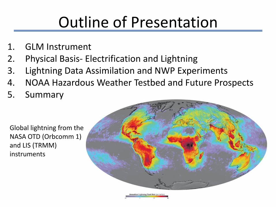
Launch Schedule

launch March 4, 2010

GOES East

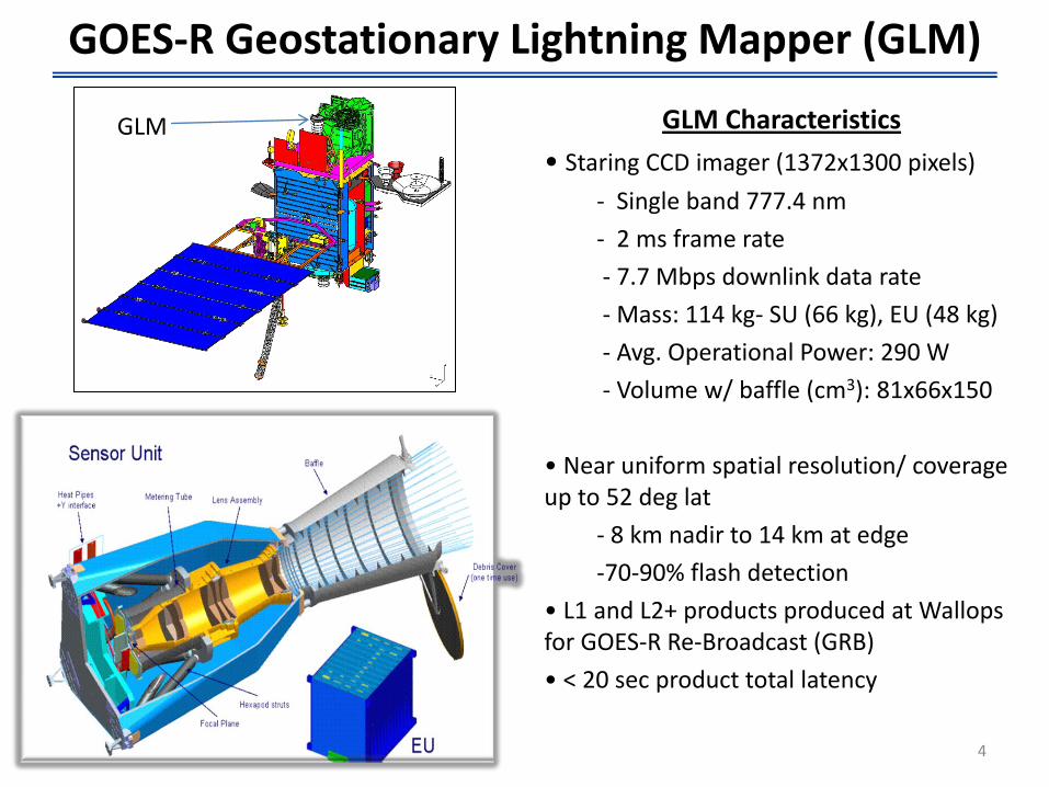
GOES-R Geostationary Lightning Mapper (GLM)

LIS/OTD 1997-2005GLM Characteristics

• Staring CCD imager (1372x1300 pixels)

- Single band 777.4 nm

- 2 ms frame rate

- 7.7 Mbps downlink data rate

- Mass: 114 kg- SU (66 kg), EU (48 kg)

- Avg. Operational Power: 290 W

- Volume w/ baffle (cm3): 81x66x150

• Near uniform spatial resolution/ coverage up to 52 deg lat

- 8 km nadir to 14 km at edge

-70-90% flash detection

• L1 and L2+ products produced at Wallops for GOES-R Re-Broadcast (GRB)

• < 20 sec product total latency

4

GLM

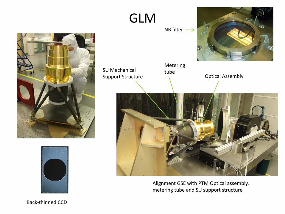
GLM

Alignment GSE with PTM Optical assembly, metering tube and SU support structure

Optical AssemblySU Mechanical Support Structure

Metering tube

Back-thinned CCD

NB filter

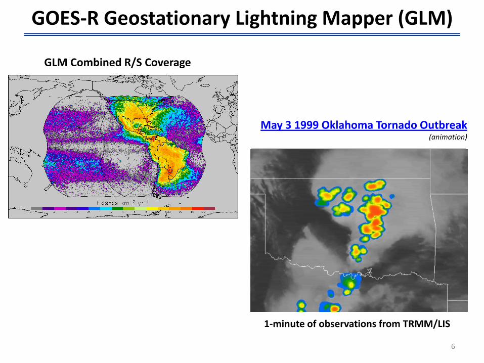
GOES-R Geostationary Lightning Mapper (GLM)

1-minute of observations from TRMM/LIS

GLM Combined R/S Coverage

May 3 1999 Oklahoma Tornado Outbreak(animation)

6

7

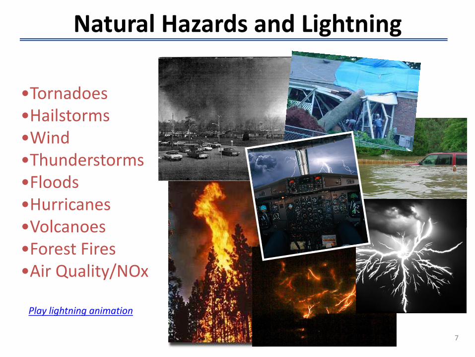
Natural Hazards and Lightning

•Tornadoes•Hailstorms•Wind•Thunderstorms•Floods•Hurricanes•Volcanoes•Forest Fires•Air Quality/NOx

Play lightning animation

8

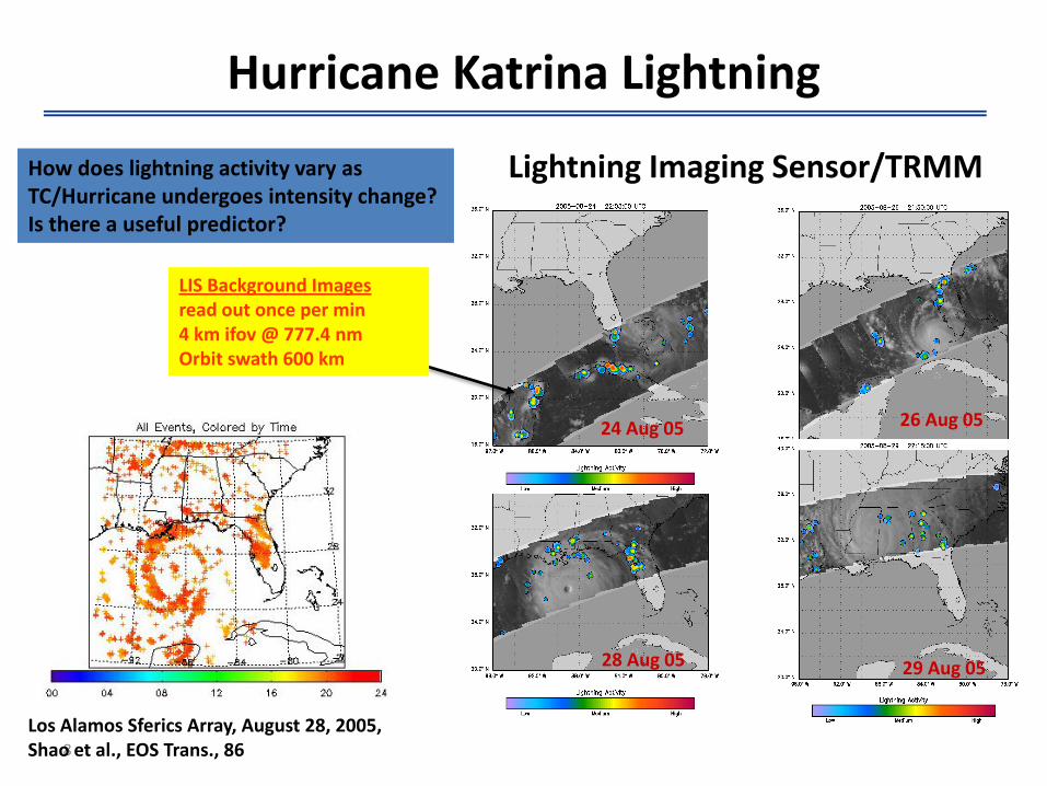
Hurricane Katrina Lightning

24 Aug 05

28 Aug 05

26 Aug 05

29 Aug 05

Los Alamos Sferics Array, August 28, 2005, Shao et al., EOS Trans., 86

How does lightning activity vary as TC/Hurricane undergoes intensity change? Is there a useful predictor?

LIS Background Imagesread out once per min4 km ifov @ 777.4 nmOrbit swath 600 km

Lightning Imaging Sensor/TRMM

99

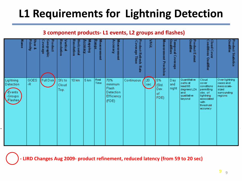
L1 Requirements for Lightning Detection

M – Mesoscale C – CONUS

H – Hemispheric

- LIRD Changes Aug 2009- product refinement, reduced latency (from 59 to 20 sec)

3 component products- L1 events, L2 groups and flashes)

Event Processing (L1B)

• An event is anything that exceeds the threshold

– Noise, Proton hit, or lightning pulse

– All events are transmitted to the ground along with housekeeping and subsampling of the background levels

– Ground processing determines which events are lightning pulses by looking for strings of pulses, both spatially and temporally (coherency)

– End-product is time-tagged, geolocated, measured, lightning (PORD Requirement)

10

11

Algorithm Overview (L2+)

• The algorithm takes input Level 1B events (time, location, amplitude) and clusters them with other events that have similar temporal and spatial characteristics

• The GLM produces a series of events (time series) which are clustered by the GLM algorithm into L2 groups and flashes, similar to the basic lightning flash data of the National Lightning Detector Network (NLDN) system (i.e., not an imager)

• The data rate from the GLM is highly variable and can range from as little as 0 events per second (when hemispheric lightning rates are very low) to perhaps as many as 40,000 events per second for very, very brief periods during widespread severe storm episodes

• The GLM algorithm must be able to process this wide dynamic range of data rates while producing output groups and flashes in under 4 seconds (verified by speed tests)

12

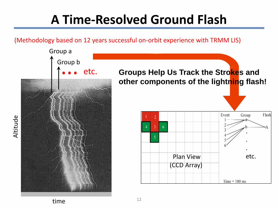
A Time-Resolved Ground Flash

time

Group a

Group b... etc.

.

.

.etc.

Alt

itu

de

Plan View(CCD Array)

Groups Help Us Track the Strokes and

other components of the lightning flash!

(Methodology based on 12 years successful on-orbit experience with TRMM LIS)

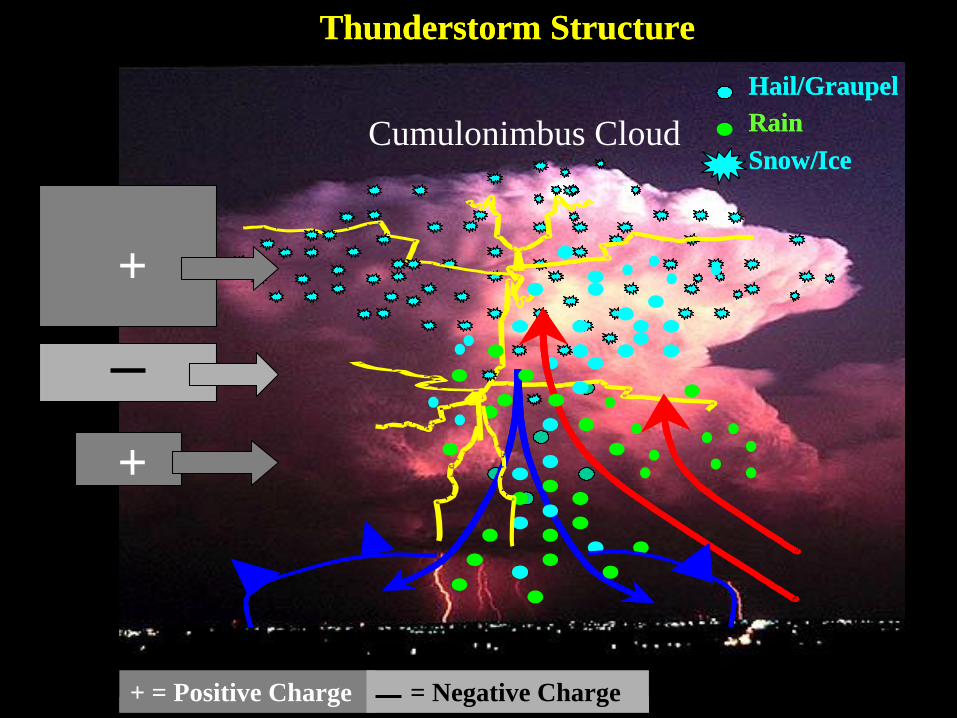
Hail/Graupel

Rain

Snow/Ice

+

+

Cumulonimbus Cloud

+ = Positive Charge = Negative Charge

Thunderstorm Structure

Hail/Graupel

Rain

Snow/Ice

Hail/Graupel

Rain

Snow/Ice

+

+

Cumulonimbus Cloud

+ = Positive Charge = Negative Charge

Thunderstorm Structure

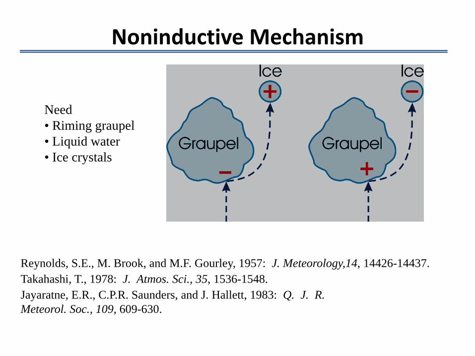
Noninductive Mechanism

Reynolds, S.E., M. Brook, and M.F. Gourley, 1957: J. Meteorology,14, 14426-14437.

Takahashi, T., 1978: J. Atmos. Sci., 35, 1536-1548.

Jayaratne, E.R., C.P.R. Saunders, and J. Hallett, 1983: Q. J. R.

Meteorol. Soc., 109, 609-630.

Need

• Riming graupel

• Liquid water

• Ice crystals

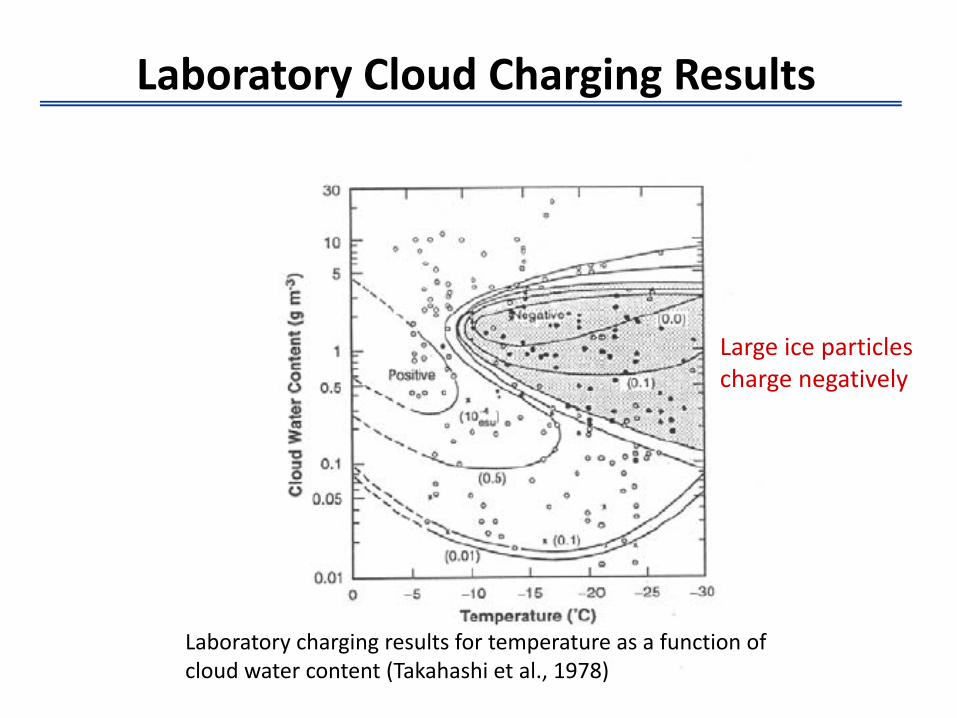
Laboratory charging results for temperature as a function of cloud water content (Takahashi et al., 1978)

Laboratory Cloud Charging Results

Large ice particles charge negatively

0 oC

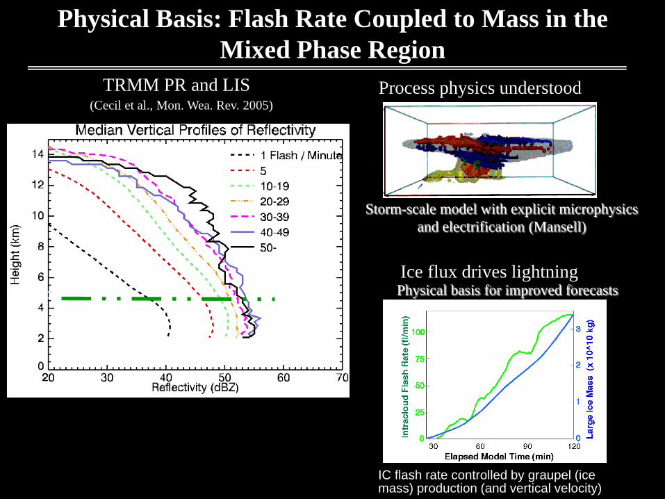
Physical Basis: Flash Rate Coupled to Mass in the

Mixed Phase Region

(Cecil et al., Mon. Wea. Rev. 2005)

Process physics understood

Storm-scale model with explicit microphysics

and electrification (Mansell)

Ice flux drives lightningPhysical basis for improved forecasts

IC flash rate controlled by graupel (ice mass) production (and vertical velocity)

TRMM PR and LIS

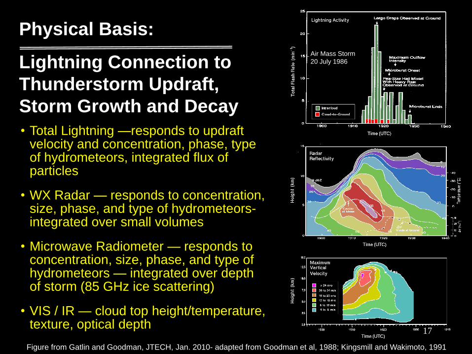
Physical Basis:

Lightning Connection to

Thunderstorm Updraft,

Storm Growth and Decay

• Total Lightning —responds to updraft velocity and concentration, phase, type of hydrometeors, integrated flux of particles

• WX Radar — responds to concentration, size, phase, and type of hydrometeors-integrated over small volumes

• Microwave Radiometer — responds to concentration, size, phase, and type of hydrometeors — integrated over depth of storm (85 GHz ice scattering)

• VIS / IR — cloud top height/temperature, texture, optical depth

Air Mass Storm

20 July 1986

17

Figure from Gatlin and Goodman, JTECH, Jan. 2010- adapted from Goodman et al, 1988; Kingsmill and Wakimoto, 1991

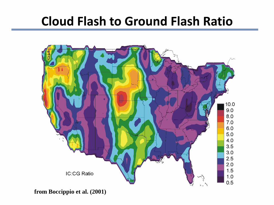
Cloud Flash to Ground Flash Ratio

from Boccippio et al. (2001)

%

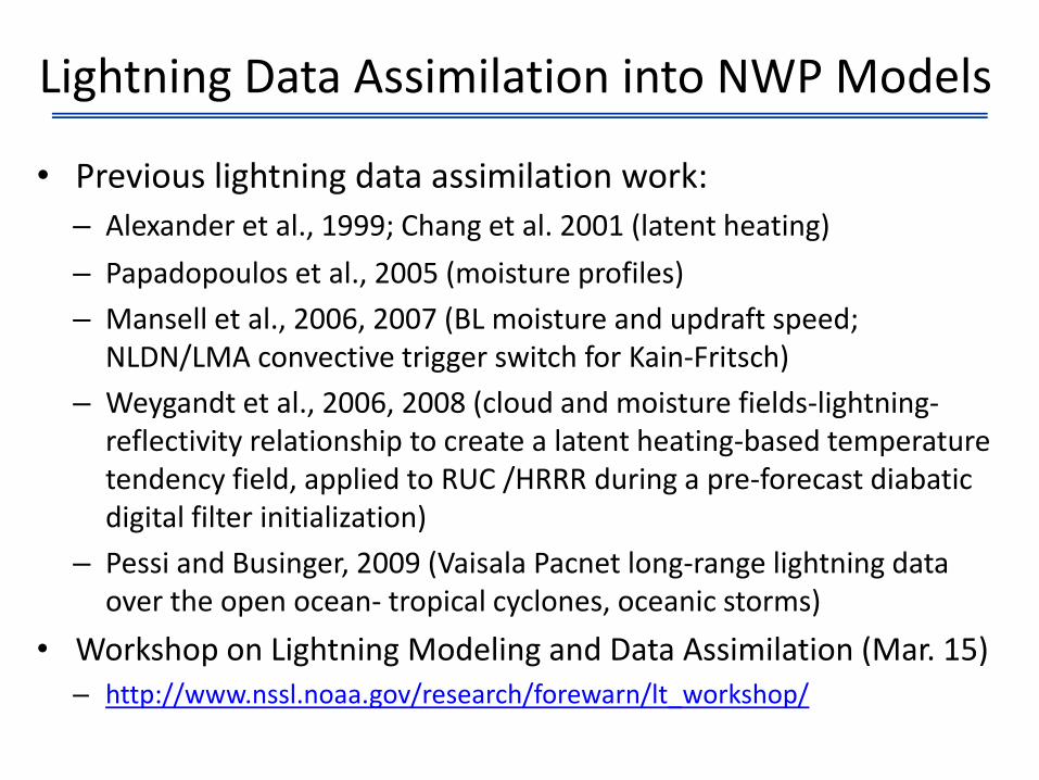
• Previous lightning data assimilation work:

– Alexander et al., 1999; Chang et al. 2001 (latent heating)

– Papadopoulos et al., 2005 (moisture profiles)

– Mansell et al., 2006, 2007 (BL moisture and updraft speed; NLDN/LMA convective trigger switch for Kain-Fritsch)

– Weygandt et al., 2006, 2008 (cloud and moisture fields-lightning-reflectivity relationship to create a latent heating-based temperature tendency field, applied to RUC /HRRR during a pre-forecast diabaticdigital filter initialization)

– Pessi and Businger, 2009 (Vaisala Pacnet long-range lightning data over the open ocean- tropical cyclones, oceanic storms)

• Workshop on Lightning Modeling and Data Assimilation (Mar. 15)– http://www.nssl.noaa.gov/research/forewarn/lt_workshop/

Lightning Data Assimilation into NWP Models

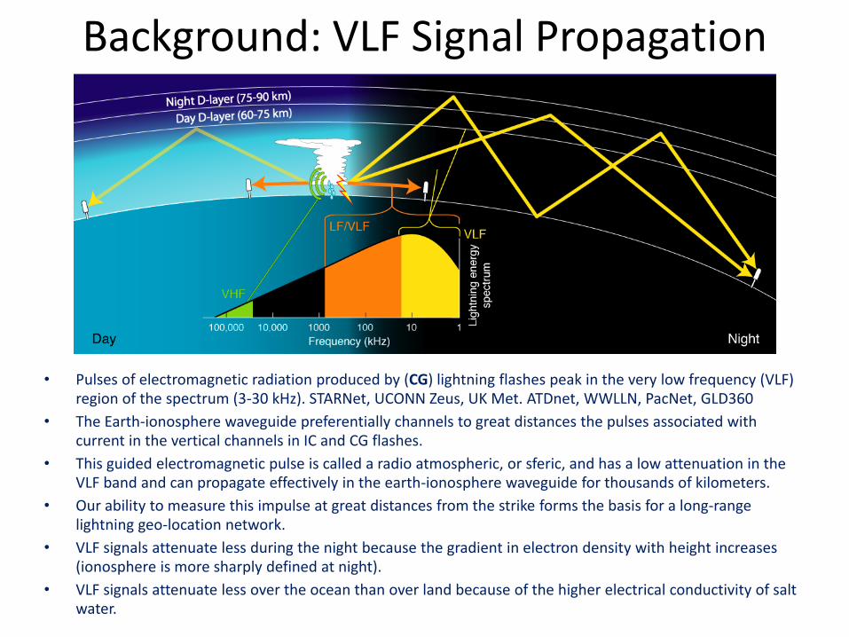
Background: VLF Signal Propagation

• Pulses of electromagnetic radiation produced by (CG) lightning flashes peak in the very low frequency (VLF) region of the spectrum (3-30 kHz). STARNet, UCONN Zeus, UK Met. ATDnet, WWLLN, PacNet, GLD360

• The Earth-ionosphere waveguide preferentially channels to great distances the pulses associated with current in the vertical channels in IC and CG flashes.

• This guided electromagnetic pulse is called a radio atmospheric, or sferic, and has a low attenuation in the VLF band and can propagate effectively in the earth-ionosphere waveguide for thousands of kilometers.

• Our ability to measure this impulse at great distances from the strike forms the basis for a long-range lightning geo-location network.

• VLF signals attenuate less during the night because the gradient in electron density with height increases (ionosphere is more sharply defined at night).

• VLF signals attenuate less over the ocean than over land because of the higher electrical conductivity of salt water.

21

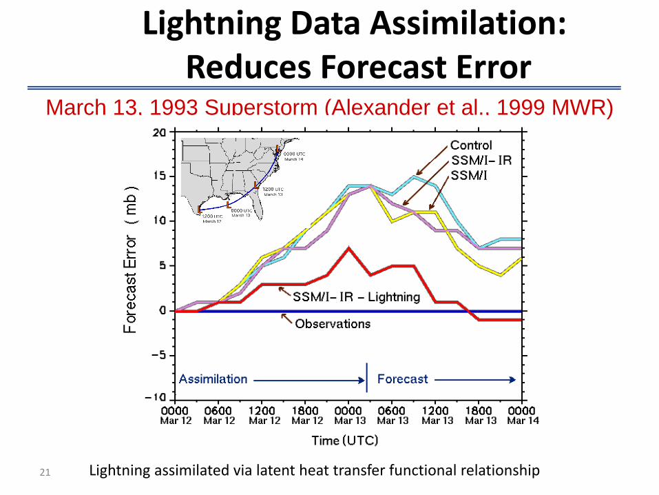
March 13, 1993 Superstorm (Alexander et al., 1999 MWR)

Lightning Data Assimilation:Reduces Forecast Error

Lightning assimilated via latent heat transfer functional relationship

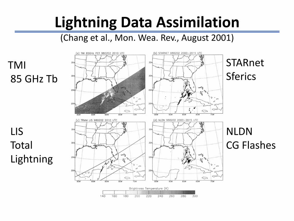
Lightning Data Assimilation(Chang et al., Mon. Wea. Rev., August 2001)

TMI85 GHz Tb

LISTotal Lightning

STARnetSferics

NLDNCG Flashes

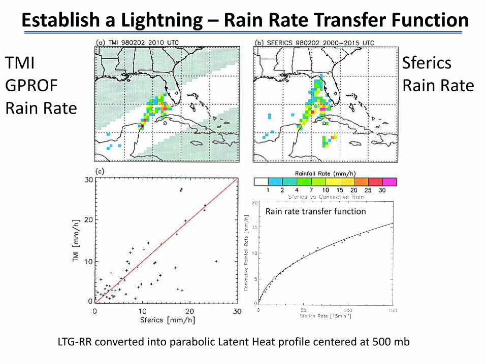
Rain rate transfer function

Establish a Lightning – Rain Rate Transfer Function

TMIGPROFRain Rate

SfericsRain Rate

LTG-RR converted into parabolic Latent Heat profile centered at 500 mb

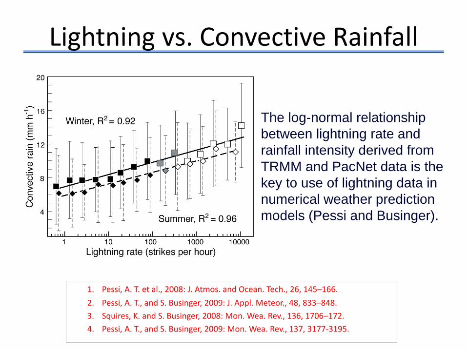
The log-normal relationship

between lightning rate and

rainfall intensity derived from

TRMM and PacNet data is the

key to use of lightning data in

numerical weather prediction

models (Pessi and Businger).

Lightning vs. Convective Rainfall

1. Pessi, A. T. et al., 2008: J. Atmos. and Ocean. Tech., 26, 145–166.

2. Pessi, A. T., and S. Businger, 2009: J. Appl. Meteor., 48, 833–848.

3. Squires, K. and S. Businger, 2008: Mon. Wea. Rev., 136, 1706–172.

4. Pessi, A. T., and S. Businger, 2009: Mon. Wea. Rev., 137, 3177-3195.

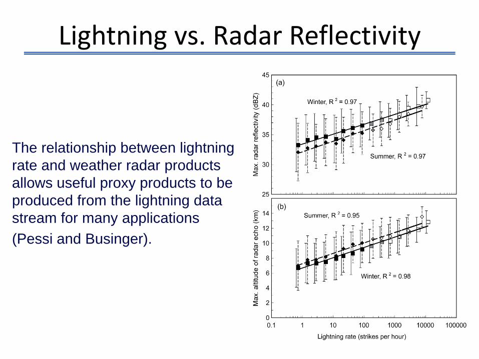
Lightning vs. Radar Reflectivity

The relationship between lightning

rate and weather radar products

allows useful proxy products to be

produced from the lightning data

stream for many applications

(Pessi and Businger).

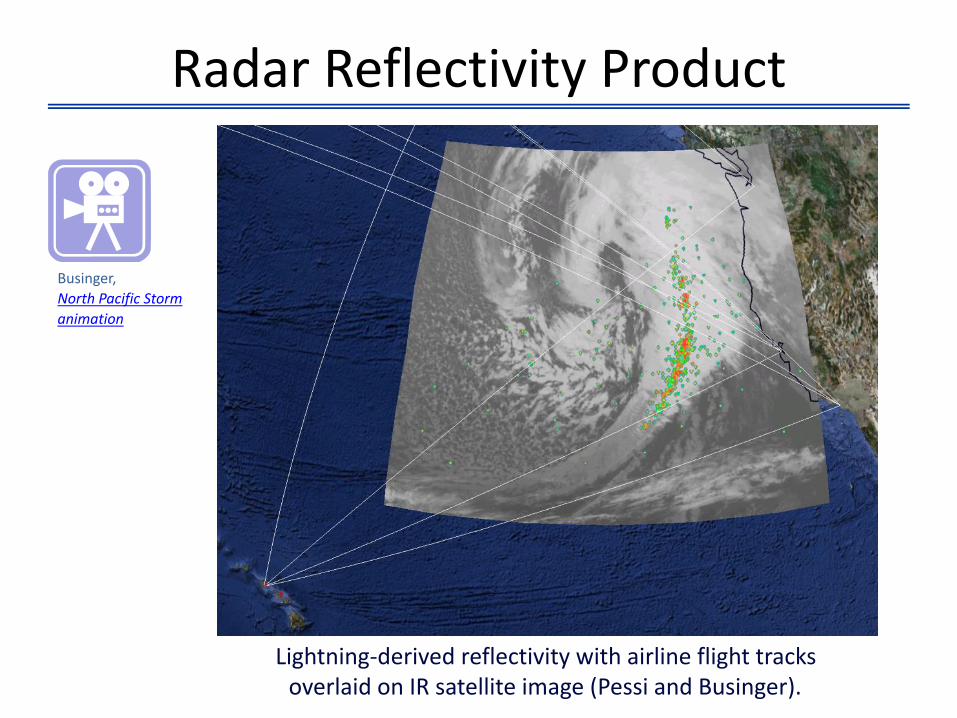
Radar Reflectivity Product

Lightning-derived reflectivity with airline flight tracks overlaid on IR satellite image (Pessi and Businger).

Businger,

North Pacific Storm

animation

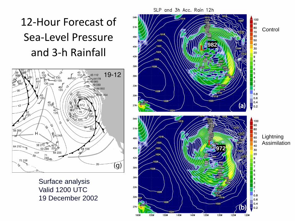
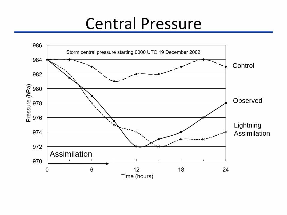
Control

Lightning

Assimilation

Surface analysis

Valid 1200 UTC

19 December 2002

L

12-Hour Forecast of

Sea-Level Pressure

and 3-h Rainfall

L972

982

Control

Observed

Lightning

Assimilation

Central Pressure

Assimilation

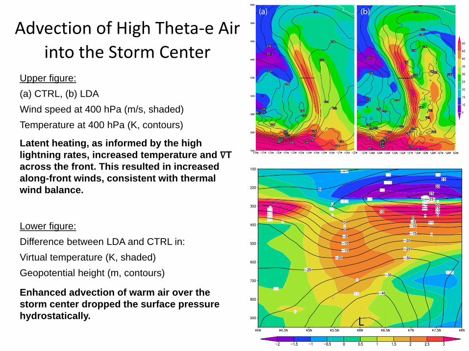
Advection of High Theta-e Air

into the Storm CenterUpper figure:

(a) CTRL, (b) LDA

Wind speed at 400 hPa (m/s, shaded)

Temperature at 400 hPa (K, contours)

Latent heating, as informed by the high

lightning rates, increased temperature and ∇T

across the front. This resulted in increased

along-front winds, consistent with thermal

wind balance.

Lower figure:

Difference between LDA and CTRL in:

Virtual temperature (K, shaded)

Geopotential height (m, contours)

Enhanced advection of warm air over the

storm center dropped the surface pressure

hydrostatically.

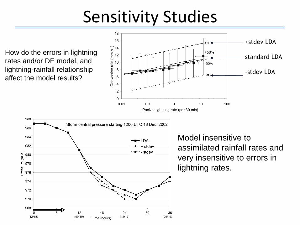
Sensitivity Studies

Model insensitive to

assimilated rainfall rates and

very insensitive to errors in

lightning rates.

How do the errors in lightning

rates and/or DE model, and

lightning-rainfall relationship

affect the model results?

+stdev LDA

standard LDA

-stdev LDA

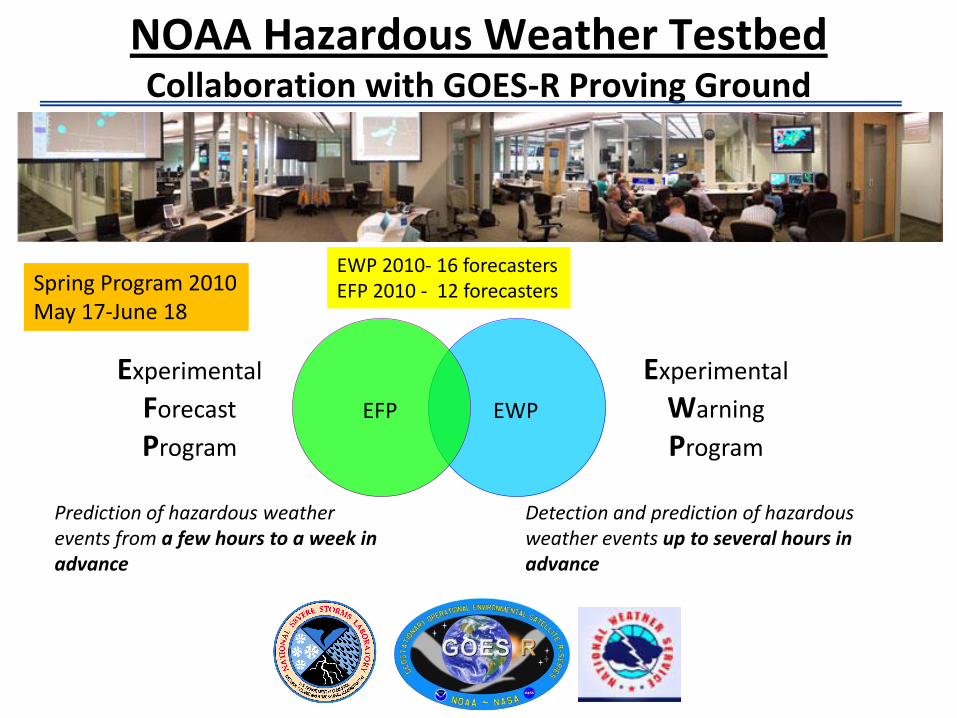
NOAA Hazardous Weather TestbedCollaboration with GOES-R Proving Ground

Two Main Program Areas…

Experimental

Warning

Program

Experimental

Forecast

Program

EFP EWP

Prediction of hazardous weather events from a few hours to a week in advance

Detection and prediction of hazardous weather events up to several hours in advance

EWP 2010- 16 forecastersEFP 2010 - 12 forecastersSpring Program 2010

May 17-June 18

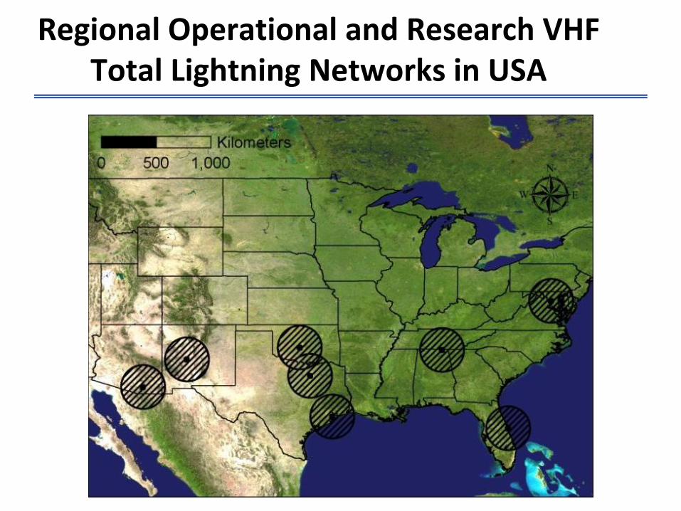
Regional Operational and Research VHF Total Lightning Networks in USA

33

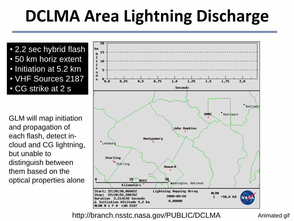
DCLMA Area Lightning Discharge

• 2.2 sec hybrid flash

• 50 km horiz extent

• Initiation at 5.2 km

• VHF Sources 2187

• CG strike at 2 s

Animated gif

GLM will map initiation

and propagation of

each flash, detect in-

cloud and CG lightning,

but unable to

distinguish between

them based on the

optical properties alone

http://branch.nsstc.nasa.gov/PUBLIC/DCLMA

34

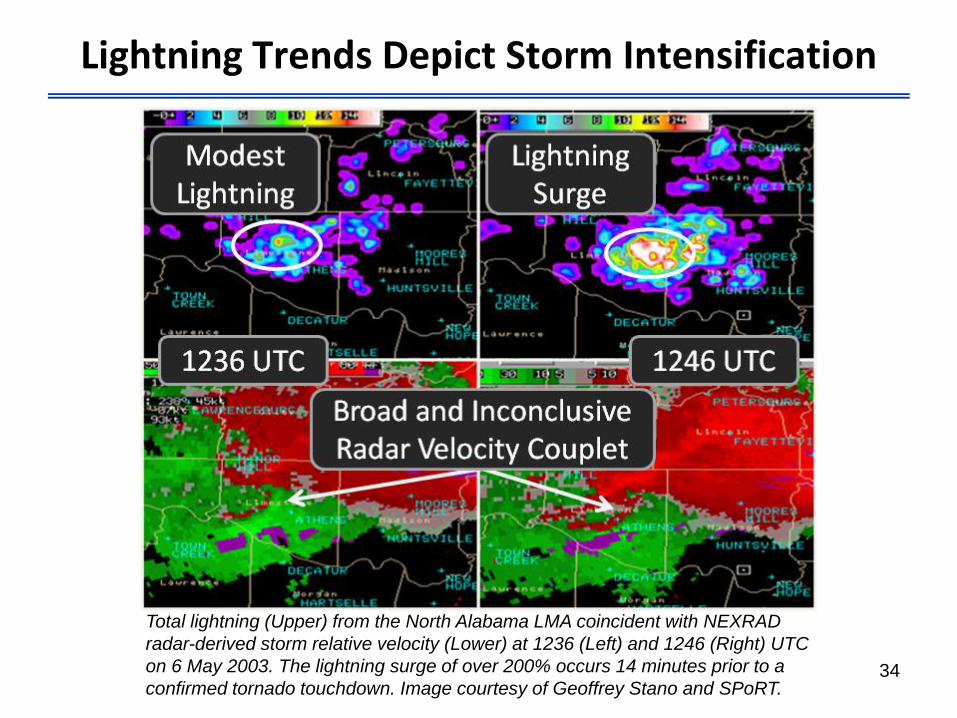
Total lightning (Upper) from the North Alabama LMA coincident with NEXRAD

radar-derived storm relative velocity (Lower) at 1236 (Left) and 1246 (Right) UTC

on 6 May 2003. The lightning surge of over 200% occurs 14 minutes prior to a

confirmed tornado touchdown. Image courtesy of Geoffrey Stano and SPoRT.

Lightning Trends Depict Storm Intensification

• High-resolution explicit convection WRF forecasts can capture the

character and general timing and placement of convective

outbreaks well;

• Traditional parameters used to forecast thunder, such as CAPE

fields, often overestimate LTG threat area; CAPE thus must be

considered valid only as an integral of threat over some ill-defined

time;

• No forward model for LTG available for DA now; thus search for

model proxy fields for LTG is appropriate;

• Research results with global TRMM data agrees with models (e.g.,

Mansell) that LTG flash rates depend on updraft, precip. ice

amounts.

35

WRF Lightning Threat Forecasts Background

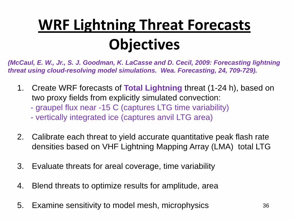
WRF Lightning Threat Forecasts Objectives

1. Create WRF forecasts of Total Lightning threat (1-24 h), based on

two proxy fields from explicitly simulated convection:

- graupel flux near -15 C (captures LTG time variability)

- vertically integrated ice (captures anvil LTG area)

2. Calibrate each threat to yield accurate quantitative peak flash rate

densities based on VHF Lightning Mapping Array (LMA) total LTG

3. Evaluate threats for areal coverage, time variability

4. Blend threats to optimize results for amplitude, area

5. Examine sensitivity to model mesh, microphysics 36

(McCaul, E. W., Jr., S. J. Goodman, K. LaCasse and D. Cecil, 2009: Forecasting lightning

threat using cloud-resolving model simulations. Wea. Forecasting, 24, 709-729).

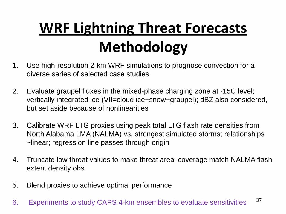
WRF Lightning Threat ForecastsMethodology

1. Use high-resolution 2-km WRF simulations to prognose convection for a

diverse series of selected case studies

2. Evaluate graupel fluxes in the mixed-phase charging zone at -15C level;

vertically integrated ice (VII=cloud ice+snow+graupel); dBZ also considered,

but set aside because of nonlinearities

3. Calibrate WRF LTG proxies using peak total LTG flash rate densities from

North Alabama LMA (NALMA) vs. strongest simulated storms; relationships

~linear; regression line passes through origin

4. Truncate low threat values to make threat areal coverage match NALMA flash

extent density obs

5. Blend proxies to achieve optimal performance

6. Experiments to study CAPS 4-km ensembles to evaluate sensitivities 37

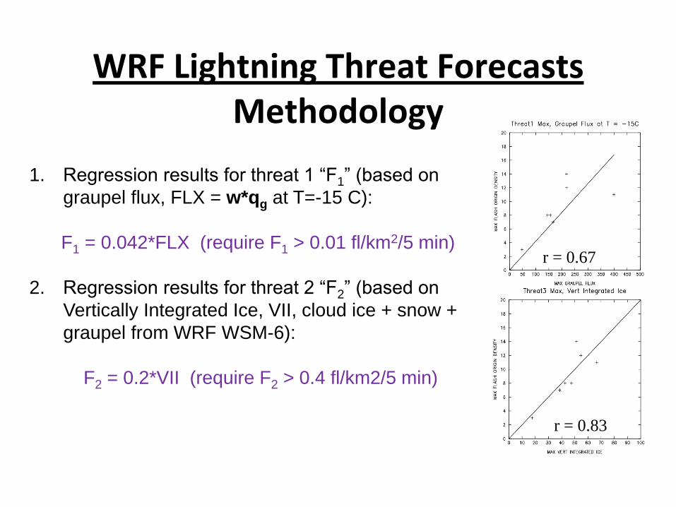
WRF Lightning Threat ForecastsMethodology

1. Regression results for threat 1 ―F1‖ (based on

graupel flux, FLX = w*qg at T=-15 C):

F1 = 0.042*FLX (require F1 > 0.01 fl/km2/5 min)

2. Regression results for threat 2 ―F2‖ (based on

Vertically Integrated Ice, VII, cloud ice + snow +

graupel from WRF WSM-6):

F2 = 0.2*VII (require F2 > 0.4 fl/km2/5 min)

38

r = 0.67

r = 0.83

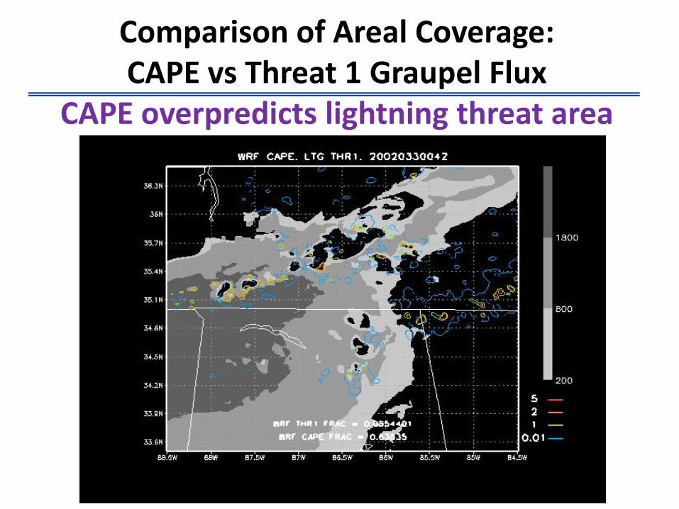
Comparison of Areal Coverage: CAPE vs Threat 1 Graupel Flux

CAPE overpredicts lightning threat area

39

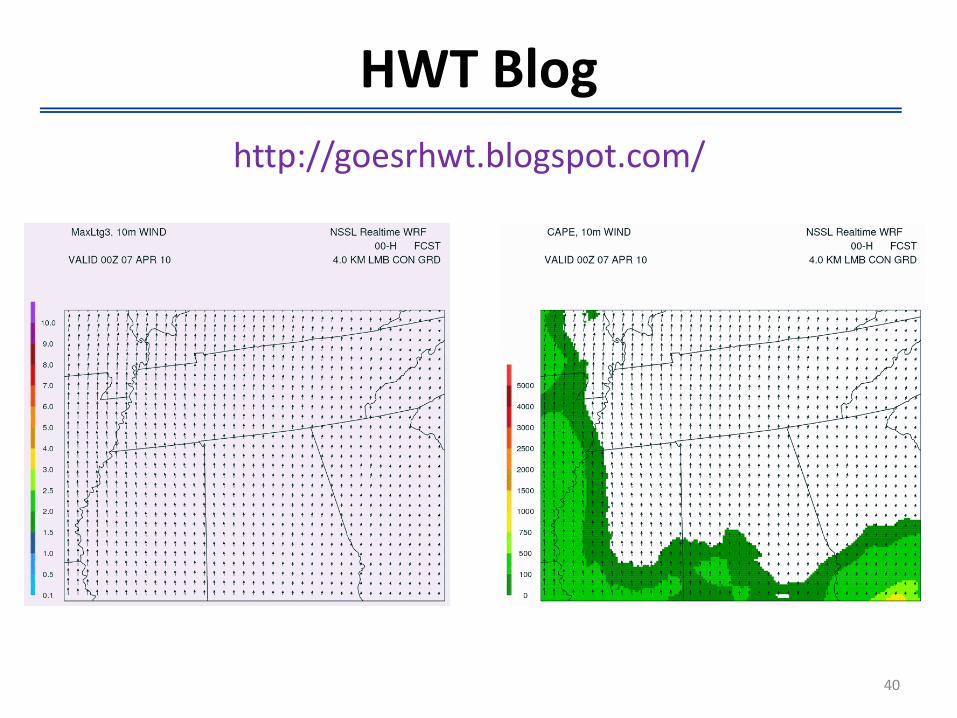
HWT Blog

40

http://goesrhwt.blogspot.com/

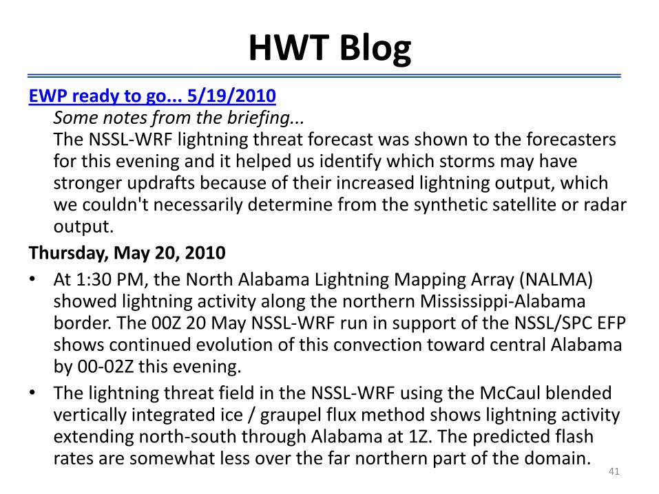
HWT Blog

41

EWP ready to go... 5/19/2010Some notes from the briefing...The NSSL-WRF lightning threat forecast was shown to the forecasters for this evening and it helped us identify which storms may have stronger updrafts because of their increased lightning output, which we couldn't necessarily determine from the synthetic satellite or radar output.

Thursday, May 20, 2010

• At 1:30 PM, the North Alabama Lightning Mapping Array (NALMA) showed lightning activity along the northern Mississippi-Alabama border. The 00Z 20 May NSSL-WRF run in support of the NSSL/SPC EFP shows continued evolution of this convection toward central Alabama by 00-02Z this evening.

• The lightning threat field in the NSSL-WRF using the McCaul blended vertically integrated ice / graupel flux method shows lightning activity extending north-south through Alabama at 1Z. The predicted flash rates are somewhat less over the far northern part of the domain.

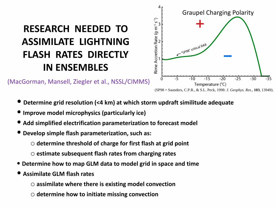
• Determine grid resolution (<4 km) at which storm updraft similitude adequate

• Improve model microphysics (particularly ice)

• Add simplified electrification parameterization to forecast model

• Develop simple flash parameterization, such as:

o determine threshold of charge for first flash at grid point

o estimate subsequent flash rates from charging rates

• Determine how to map GLM data to model grid in space and time

• Assimilate GLM flash rates

o assimilate where there is existing model convection

o determine how to initiate missing convection

RESEARCH NEEDED TOASSIMILATE LIGHTNINGFLASH RATES DIRECTLY

IN ENSEMBLES

Graupel Charging Polarity

(SP98 = Saunders, C.P.R., & S.L. Peck, 1998: J. Geophys. Res., 103, 13949).

(MacGorman, Mansell, Ziegler et al., NSSL/CIMMS)

Summary

• GLM instrument development on schedule– EDU risk reduction completion summer 2010

– FM 1 optical component long lead items in procurement

– Full CDR Fall 2010

• Ver. 1 of ATBD, Val Plan, Proxy Data, L2 Prototype S/W– Product demonstrations at NOAA Testbeds

• Hazardous Weather Testbed (2010 Spring Program with VORTEX-II IOP, Summer Program)

• Joint Hurricane Testbed (NASA GRIP, NSF PREDICT)

• Aviation Weather Testbed (NextGen)

• Continue Regional WFO demonstrations (Norman, Huntsville, Sterling, Melbourne, …)

• New Risk Reduction/Advanced Product Initiatives– Data Assimilation: JCSDA FFO 2010 funding two new GLM investigations

– High Impact Weather Working Group- GOES-R DA focus on short-range NWP

– Combined sensors/platforms (e.g., ABI/GLM ; ABI/GLM/GPM)

– GLM proxy data 12-mo. campaign in Sao Paulo in partnership with InPE and CHUVA GPM pre-launch ground validation program

– NSF Deep Convective Cloud and Chemistry (DC3) Experiment 2012