The geometry of the double gyroid wire network: …ebkaufma/JCommGeom6_12.pdfThe geometry of the...

J. Noncommut. Geom. 6 (2012), 623–664DOI 10.4171/JNCG/101

Journal of Noncommutative Geometry© European Mathematical Society

The geometry of the double gyroid wire network:quantum and classical

Ralph M. Kaufmann, Sergei Khlebnikov, and Birgit Wehefritz-Kaufmann

Abstract. Quantum wire networks have recently become of great interest. Here we deal with anovel nano material structure of a double gyroid wire network. We use methods of commutativeand noncommutative geometry to describe this wire network. Its noncommutative geometryis closely related to noncommutative 3-tori as we discuss in detail.

Mathematics Subject Classification (2010). 46L60, 81R60, 58B34, 53A10, 57M15, 52C07,05C38, 81Q10.

Keywords. Double gyroid, noncommutative geometry, K-theory, traces, Harper operator, graphHamiltonian, noncommutative Brillouin zone, lattices, lattice differential operator, quantumgraph, fundamental group, magnetization, projective representations, minimal loops, honey-comb lattice, hexagonal lattice.

Introduction

Interfaces that can be modeled by surfaces of constant mean curvature (CMC) areubiquitous in nature and can now be synthesized in laboratory. Recently, Urade et al.[23] have reported fabrication of a nano-porous silica film whose structure is relatedto a specific CMC surface: the gyroid. The structure is three-dimensionally periodicand has three components:1 a thick surface and two channels, as detailed below. Theinterface between the wall and the channels approximates a double gyroid.

Urade et al. [23] have also demonstrated a nanofabrication technique in whichthe channels are filled with a metal, while the silica wall can be either left in placeor removed. These novel materials open a wide field of applications due to theirtopological and geometric features. The channels are a few nanometers wide and,when filled with a conducting or semiconducting material, are expected to acquirecertain characteristics of one-dimensional quantum wires (such as a blueshift of thespectrum and an enhanced density of states), while remaining three-dimensional inother respects [13]. Geometrically, the one-dimensional structure appears since eachof the channels can be retracted to a skeletal graph [8], the gyroid graph.

1And so is sometimes referred to as tri-continuous.

624 R. M. Kaufmann, S. Khlebnikov, and B. Wehefritz-Kaufmann

We will concentrate on the resulting geometry and topology of these networksin the possible presence of a constant magnetic field. Topological quantities are ofparticular physical interest as they remain stable under continuous perturbations. Inpractice, those should be small as not to break the structure.

We use two approaches: the first is purely classical and the second is the quan-tum/noncommutative approach due to Alain Connes [5]. The classical results weprovide are a study of the fundamental group of the channel. Here we determine thefundamental group of each channel system. This group is the commutator subgroupof the free group in three generators. A surprising result coming directly from thegyroid geometry is that there is a new length function on the free group which isdifferent from the ordinary word length. With the help of this length function wedetermine the shortest loops at any given point. There are 15 such topologically dis-tinct shortest loops (30 if one includes orientation). They split into two groups whichare distinguished by their cyclic symmetry which is either of order two or three. Inboth groups there are three generators using this additional symmetry. These loopsare of particular interest since numerical simulations [13] show the possibility of anenhanced density of states in a double-gyroid quantum wire, due to states that arenearly localized near such loops. We also calculate the flux of a constant magneticfield through these loops. The tool is an effective unit vector. The result of thecalculation is that these effective unit vectors have a particularly simple form (seeTable 1). This fact should also be relevant for the study of the spin-orbit coupling ofthe loop-localized states.

Our study of the noncommutative geometry is motivated by one of the big earlysuccesses of the noncommutative geometry of Alain Connes. This was the descrip-tion by Bellissard et al. of the quantum Hall effect [3]. It allowed to explain theinteger effect in terms of the noncommutative geometric properties. The underlyinggeometry in that situation is the quantum 2-torus. Recently there have been furtheranalyses on the fractional effect using hyperbolic geometry as a model [15]. Theconceptual approach as outlined in [2] is to replace the Brillouin zone by a noncom-mutative Brillouin zone which is given by a C*-algebra that contains the translationalsymmetry operators and the Hamiltonian. In this geometry relevant quantities canoften be expressed in terms of the K-theory of this algebra. This Abelian group cap-tures information related to the topology or better the homotopy type of the algebraor geometric setup. These are again quantities which are stable under continuousdeformations. A prime example is the Hall conductance.

A general fact, which is pertinent to our discussion, is that the K-groups alsoserve to label the gaps in the spectrum. Roughly this goes as follows. Given a gapin the spectrum there is a projector projecting to the energy levels below the gap.This projector in turn gives rise to a K-theory element. If one knows the orderedK-theory, then one can also sometimes deduce if only finitely or infinitely many gapsare possible.

In our situation, we determine the said C*-algebra for one channel in the presenceof a magnetic field and describe the K-theories. The Hamiltonian we use is the

The geometry of the double gyroid wire network 625

generalization [20], [2] of the Harper Hamiltonian [12], [2] adapted to our situation.2

We call the resulting algebra the Bellissard–Harper algebra and denote it by B. Thisgeometry is closely related to the noncommutative 3-torus T 3

‚. Here ‚ is a skew-symmetric .3� 3/-matrix determined by the magnetic field. In fact we show that thealgebra is isomorphic to a subalgebra of the .4 � 4/-matrix algebra with coefficientsin the noncommutative 3-torus. By varying the magnetic field, we obtain a three-parameter family of algebras. We prove that at all but finitely many points thisalgebra is the full matrix algebra and hence Morita equivalent to T 3

‚. Since T 3‚ is

simple at irrational ‚, one would expect this to be true on a dense set (see §3). Wenot only prove that this expectation holds at the irrational points, but we are able toextend this result to almost all rational points. At certain special values of the fieldwhich we enumerate, however, the algebra is genuinely smaller, leading to a possiblydifferent K-theory. At these points the material may also exhibit special properties.

The ordered K-theory of the 3-torus is completely known [18], [17], [6] andactually completely classifies the isomorphism classes of such tori [19], [7]. Ouralgebra always injects into a T 3

‚. From this and the knowledge of the ordered K-group of the noncommutative torus, we obtain the result that there are only finitelymany gaps possible at rational values of ‚.

Our approach to both the classical and the quantum geometry uses graph-theoret-ical methods. The relevant graphs are the gyroid graph which is a 3-regular graphand its quotient under the translation symmetry group. In order to give the matrixalgebras explicitly we introduce the notions of a graph representation. Using rootedspanning trees, we are able to represent the algebra B in terms of matrices, wherethey are amenable to direct computations.

As the geometry of the gyroid and its channels is quite difficult, we also treat thehoneycomb lattice as a two-dimensional analogue. Indeed, the gyroid lattice graph(the graph onto which each channel retracts) is in many ways the three-dimensionalanalogue of the honeycomb lattice, which is why when developing the more generalparts of the theory we will in parallel consider these two cases as our main examples.Both graphs are 3-regular, and both of the graphs are not mathematical lattices butonly physical lattices.3 This means that they give rise to two groups, one which isthe space or symmetry group and the other is the group of the lattice, of which theycan be considered a subset. In the honeycomb case these are both Z2 but embeddedinto R2 as the triangular lattice and its dual. For the gyroid the groups are bothZ3, but they are embedded as a body centered cubic (bcc) and a face centered cubic(fcc) lattice in R3, which are again dual to each other. Furthermore the fundamentalgroup of the honeycomb lattice is the commutator subgroup of the free group on twoelements, while for the gyroid �1 is the commutator subgroup of the free group inthree generators. And in both cases we find a new length function on the free groupinduced by the geometry of the lattice.

2The generalized Harper operator is also the operator underlying the noncommutative geometry of thequantum Hall effect [3], [15].

3See §3.2 for the disambiguation of the use of the word “lattice”.


The paper is organized as follows:In the first section, we start with a review of the classical geometry of the gyroid

and then prove the results on the fundamental group and the smallest loops. In thesecond section, we formally introduce graphs and lattices and the relevant groupsassociated to them. We then define their representation in Hilbert spaces and theassociated Harper operators. Finally, we show how to obtain a matrix representationof B using rooted spanning trees. In the third section, we apply the general theoryof the second section to the noncommutative geometry of a lattice using a Harperoperator, detailing the honeycomb and the gyroid case. Here we also briefly reviewprojective representations and explain how they arise in the presence of a magneticfield. In this context, we can already show that there can only be finitely many gapsfor the gyroid at rational ‚. We also outline the general approach to calculating B

and its K-theory and the expected results. In particular, we compute the K-theory inthe commutative case in terms of a cover of a torus.

In the last section we apply the outlined strategies to calculate the algebras B andtheir K-theory for Bravais lattices, the honeycomb lattice and the gyroid lattice graph.

1. The classical geometry of the double gyroid

1.1. The double gyroid and its channels. The gyroid is an embedded CMC surfacein R3 [9]. It was discovered by Alan Schoen [21]. In nature it was observed as aninterface for di-block co-polymers [10], [22]. The interface actually consists of twodisconnected surfaces. Each of them is a gyroid surface. The double gyroid (DG) isa particular configuration of two mutually non-intersecting embedded gyroids.

A single gyroid has symmetry group I4132 while the double gyroid has thesymmetry group Ia N3d where the extra symmetry comes from interchanging the twogyroids.4

Since CMC surfaces are mathematically hard to handle level surfaces have beensuggested as a possible approximation in [14]. The level surface approximation forthe double gyroid again consists of two level surfaces. We will call the two surfaceinterfaces S1 and S2. For the discussion at hand it is not relevant if the two surfacesare actually the CMC surfaces or their level surface approximations. One exampleof a DG approximation is given by the family of level surfaces [14]

Lt W sin x cosy C sin y cos z C sin z cos x D t:

A model for the double gyroid is then given by Lw and L�w for 0 � w <p2.

The complement R3 n G of a single gyroid G has two components. These com-ponents will be called the gyroid wire systems or channels.

4Here I4132 and Ia N3d are given in the international or Hermann–Mauguin notation for symmetrygroups; see e.g. [11].


There are two distinct channels, one left and one right handed. Each of thesechannels contracts onto a graph, called skeletal graph in [21], [8]. We will call thesegraphs �C and ��. Each graph is periodic and trivalent. We fix �C to be the graphwhich has the node v0 D .5

8; 5

8; 5

8/. We will give more details on the graph �C below.

The channel containing �C is shown in Figure 1. A (crystal) unit cell of thechannel together with the embedded graph �C is shown in Figure 2 and just the graphis contained in Figure 3.

0.00.5

1.01.5

2.0

0.00.5

1.01.5

2.0

0.0

0.5

1.0

1.5

2.0

Figure 1. The channel CC.

v0

v1

v2

v3

v4

v5

v6

v7

0.00.5

1.0

0.0

0.5

1.00.0

0.5

1.0

Figure 2. The graph �C embedded into its channel CC.


v0

v1

v2

v3

v4

v5

v6

v7

0.00.5

1.0

0.0

0.5

1.00.0

0.5

1.0

Figure 3. The graph �C.

In constructing the surface, one can actually start with one of these graphs andevolve the surface from it [8]. The symmetry of one skeletal graph is that of a singlegyroid I4132.

To obtain the double gyroid one can evolve from both the graphs. The commonsymmetry group of both of these graphs is Ia N3d . This symmetry group can actuallybe defined already on the nodes V˙ of the two graphs �˙. The subgroup I4132 isthen determined to be the subgroup that fixes both sets of nodes (setwise).

In the case of the double gyroid S D S1 q S2, the complement C D R3 n S ofthe disjoint union of the two gyroid surfaces has three connected components. Theseare two channel systems CC and C�, each of which can be retracted to its skeletalgraph �˙. In fact, the skeletal graph is a deformation retract [8]. There is a thirdconnected component F and we will write xF D F [ S . This is a 3-manifold withtwo boundary components, more precisely, @ xF D S D S1 q S2. F can be thoughtof as a “thickened” (fat) surface. The thickness is fixed by the parameter w. Notethat F can be retracted to each of the two boundary surfaces Si . In fact there is adeformation retract of F onto the gyroid.

This means that all homotopical information about the complements of the doublegyroid is encoded in the gyroid/level surface and the two skeletal graphs.

The translational symmetry group for both the gyroid and the double gyroid is theBravais lattice bcc. Note that we will usually use “lattice” in the physical terminology,e.g. speak about the honeycomb lattice. The term “Bravais lattice” will be used todenote a maximal rank mathematical lattice, i.e., a free rank n Abelian subgroup ofRn. In order to preempt any confusion, we give precise definitions for our terminologyin §3.2.


1.2. The skeletal graph

1.2.1. The vertices and edges. We will now describe the graph �C embeddedinto R3.

Set

v0 D �58; 5

8; 5

8

�; v4 D �

78; 5

8; 3

8

�;

v1 D �38; 7

8; 5

8

�; v5 D �

18; 7

8; 3

8

�;

v2 D �38; 1

8; 7

8

�; v6 D �

18; 1

8; 1

8

�;

v3 D �58; 3

8; 7

8

�; v7 D �

78; 3

8; 1

8

�;

and let xVC D fv0; : : : ; v7g.Furthermore Z3 acts on R3 by translations and we let VC D Z3. xVC/ be the image

of the set xVC under this action. We will sometimes call this set of points the gyroidlattice.

Given two points v;w 2 R3 let vw D f.1 � t /v C tw j t 2 Œ0; 1�g be theline segment joining them. Also given a point v we let Tx.v/ D v C .1; 0; 0/,Ty.v/ D v C .0; 1; 0/, Tz.v/ D v C .0; 0; 1/ be the translated points.

Consider the following set of line segments

xE D fv0v1; v0v3; v0v4; v2v3; v4v7; v1v5;

v4 Tx.v5/; v7 Tx.v6/; v1 Ty.v2/;

v5 Ty.v6/; v2 Tz.v6/; v3Tz.v7/g:(1)

Let EC D Z3. xE/, where again Z3 � R3 acts as a subgroup of the translationgroup.

Definition 1.1. The graph �C is the graph whose vertices are VC, whose edges areEC with the obvious incidence relations.

We recall:

Proposition 1.2 ([8]). CC can be deformation retracted onto the graph �C and �Cis the component of the critical graph contained in CC.

Corollary 1.3. The homotopy type of the complement T D R3 n G is the same asthat of two copies of �C. In particular each channel has the same homotopy typeas �C.

This implies that all topological invariants C˙ which are homotopy invariant areisomorphic to those of �C. In particular, this means all homology, homotopy andK-groups of the topological space CC or C� are determined on �C.


1.3. The quotient graphs. Quotienting out by either the standard translation groupor the bcc lattice, we obtain the following two quotient graphs.

1.3.1. Crystallographic quotient graph. Let x�crystalC be the graph �C=Z3 thought

of as an abstract graph. This graph has a natural map embedding into the 3-torusR3=Z3.

Proposition 1.4. x�crystalC is a cube embedded into the 3-torus. More precisely the

vertices of x�crystalC are xV and the edges are the images of xE in R3=Z3.

The abstract graph is given in Figure 4 which also contains the images of thevectors ei which name and orient all edges.

0

4

3

5

2

7 6

1

e1

e1

e2

e2

e3

e3

e4

e4

e5

e5

e6

e6

Figure 4. The graph x�crystalC

for the gyroid.

Proof. Since all the vertices in the fundamental domain do not lie on the boundary,they give exactly the representatives of V in R3=Z3. The classes of the edges E�C

are given exactly by the images of the set xE in R3=Z3.

1.3.2. The (maximal) quotient graph. By modding out by Z3, we have not yet usedthe full translational symmetry of �C which is the bcc lattice. A set of generators forthe bcc lattice is

f1 ´ .1; 0; 0/; f2 D .0; 1; 0/; f3 ´ 12.1; 1; 1/ (2)

another set of generators which is more symmetric and we will use later on is:

g1 D 12.1;�1; 1/; g2 D 1

2.�1; 1; 1/; g3 D 1

2.1; 1;�1/: (3)

We letL D L.�C/ be the free Abelian subgroup of R3 generated by these vectors.We define x�C to be the abstract quotient graph �C=L.


Proposition 1.5. x�C is the graph with four vertices and six edges, where all pairs ofdistinct vertices are connected by exactly one edge.

This graph is sometimes also called the complete square. Its incidence matrix hasentries one everywhere except on the diagonal, where the entries are zero. This graphis shown in Figure 5.

AA

BB CC

DD

e1

e2

e3

e4

e5

e6

˛1 ˛3

˛2

Figure 5. The complete square, the rooted spanning tree � (root A and edges e1, e2, e3) andthe vectors corresponding to the oriented edges, the collapsed tree x�C=� .

Proof. We see that there is an embedding of Z3 � L, where L is the bcc lattice, sothat we only have to divide x�crystal

C by the additional symmetry generated by d ´12.1; 1; 1/. Now mod Z3, T 2

dŠ id and Td (the translation by d ) simply interchanges

the vertices of x�crystalC as follows: v0 $ v6, v1 $ v7, v2 $ v4 and v3 $ v5. Hence

we are left with four vertices, and we can choose the representatives v0; : : : ; v3.Checking the list of edges (1) one sees that indeed the twelve edges form pairs andone can choose the representatives vivj ; i ¤ j , i; j D 0; : : : ; 3.

Notice that this corresponds to a Z=2Z symmetry of the graph x�crystalC . It is

given by mapping each vertex to its diagonally opposite vertex and maps the edgesaccordingly.

1.4. The underlying group and lattice. There is another Bravais lattice hidden inthe geometry of the gyroid. This is the fcc lattice. The nearest neighbor positionsdiffer by vectors generating an fcc lattice.

This means in particular that after shifting by v0 the positions of the vertices of�C all lie on an fcc lattice.

In order to fix notation set

e1 D v1 � v0; e2 D v3 � v0; e3 D v4 � v0;

e4 D v3 � v2; e5 D v7 � v4; e6 D v5 � v1:(4)


Definition 1.6. Let T .�C/ be the group of R3 that is generated by

e1 D 1

4

0@�11

0

1A ; e2 D 1

4

0@ 0

�11

1A ; e3 D 1

4

0@ 1

0

�1

1A

e4 D 1

4

0@110

1A ; e5 D 1

4

0@ 0

�1�1

1A ; e6 D 1

4

0@�10

�1

1A :

Proposition 1.7. The group T .�C/ is isomorphic to Z3. The Bravais lattice itgenerates is a face centered cubic ( fcc).

Proof. There are relations among the ei given by

e1 D �e5 C e6; e2 D �e4 � e6; e3 D e4 C e5 (5)

so that we see that e3, e4, e5 are generators. These vectors are linearly independentover Z since they are independent over R. Hence they provide a free basis and anisomorphism to Z3. The vectors e4, �e5, �e6 are the standard primitive vectors forthe face centered cubic.

Of course there are many other choices of basis here, e.g. fe2; e4; e6g.

Proposition 1.8. The vertices of �C translated by �v6 lie on the three-dimensionalface centered cubic lattice generated by e4, e5, e6.

Proof. �C is path connected and we take v6 as the base point. Each line segmentsin E corresponds to an edge. Choosing an orientation for this edge defines a vector.Now the statement follows from the fact that the vectors corresponding to the linesegments in E and hence those of E�C

are exactly the vectors ˙e1; : : : ;˙e6.

1.5. Fundamental groups, loops and effective normal vectors. There is certaingeometric information which can even already be read off from the simple graph x�C.Such as its fundamental group or the minimal loops starting at a given vertex. A loopon �C is minimal if it passes through a minimal number of edges. A more generaltreatment will be given in §3.

Proposition 1.9. Let F3 be the free group in three variables. The (realization) of thegraphs �C and x�C have following fundamental groups:

(1) �1.�C/ D ŒF3; F3�,

(2) �1.x�C/ D F3.

In particular �C is the maximal Abelian cover of x�C.Since �C is homotopic to one channel, these results hold for each channel of the

gyroid.


Proof. We start with x�C. This graph is homotopic to the wedge product of threeS1’s, whence the second claim follows.

In view of Lemma 1.10 below (more generally by Proposition 3.5), we see that�1.�C/ is the subgroup that is the kernel of the map F3 to its Abelianization. Indeedthe sum of powers of each of the generators in a word in the group has to be zero,which precisely means that such a word is in the kernel of the Abelianization map orin other words, the commutator group.

Lemma 1.10. A loop on the graph x�C lifts to a loop on �C if and only if each edgeis traversed the same number of times in each direction.

Proof. The “if” direction is clear since this means that the translations have to addup to zero. The equivalence follows from the general Proposition 3.5 by noticing thatindeed the lifts l1 D e2e

�16 e�1

1 , l2 D e1e�15 e�1

3 , l3 D e3e4e�12 give rise to the vectors

Eli D fi of (3) and are linearly independent.

Proposition 1.11. There are closed loops in the graph �C. Each minimal loop goesthrough 10 sites and at each point there are 30 oriented minimal loops or 15 suchundirected loops.

Proof. A path in which one goes back and forth through an edge is homotopic to thepath in which this step is omitted. By direct calculation one can see that such a pathis given by traversing any five of the six edges. At the first step one has three choicesof edges, at the second step there are two and then again two possibilities. Here oneeither returns to the original vertex or not. In the first case there are 2 completions, andin the second case three completions to a minimal loop. Thus we have 2 � 3 � 5 D 30

possibilities. A detailed version of this enumeration is provided at the end of thissection in §1.5.1.

1.5.1. Explicit calculation of the loops. Here we give the details of the calculationof the loops. Using Proposition 3.5, we have to look for paths that traverse each edgethe same number of times. We first look at the cases where each edge is traversedonly once in each direction. We call such a path a good path. We also have to keepthe number of these edges minimal. This already puts a simple constraint on the path.We may not go back and forth through the same edge. Starting at the given vertex wehave to pass through two distinct edges. After this we have a choice, we can eithergo back to the starting vertex (case I) or we can go to the only vertex which we havenot reached yet (case II). In case I the next oriented edge is fixed, but then we havetwo choices Ia and Ib. After this we have already used five edges so that the minimalpossible number of oriented edges and hence the length of the loop is 10. Indeed, wecan complete the edge path uniquely to a good path without traversing the 6th edge.

In case II the fifth oriented edge for a good path is fixed, going opposite thefirst oriented edge. There is a choice for the sixth oriented edge in the path. Either


returning to vo (IIb) or not (IIa). The case IIb has a unique choice for a fifths orientededge for a good path and this has a unique completion to a good path involving fiveedges, again giving a loop of length 10. In case IIa, we again have two choices for thefifth oriented edge (IIa1) and (IIa2). Both these choices have a unique completionsto good paths again of length 10.

IIb

I II

Ia Ib

IIa IIa1 IIa2

Figure 6. The combinatorial cases for the minimal loops of the gyroid.

It remains to treat the cases where an edge is traversed more that once in eachdirection. Since we are not allowed to go back and forth on one edge the choices forthe first three oriented edges are as above. Now in case I we could go along the firstoriented edge again, but this would lead us to traverse at least six edges and hencewould not be minimal. At the next step of case I the choices are precisely Ia or Ib andtraversing an edge twice in the same direction would not be minimal. For case II, thefirst stage where one could use an oriented edge twice for IIa is the fifth edge. Butthen one would need at least six edges counting multiplicities. After fixing the fifthoriented edge one can only increase the number of traversed oriented edges by notchoosing a good path. Finally in case IIb again the first edge with a choice to traversean edge twice in one orientation is at the fifth oriented edge, but as before this wouldlead to a path of length greater than 10.

So all in all we have 2 � 3 D 6 choices for the first two edges and then once theseare fixed 5 choices for a good path. This means in all there are 30 such oriented paths.


1.5.2. Explicit loops. On the graph x�C there is a symmetry group of order 6 pre-serving the base point and the spanning tree � which permutes the vertices B , C andD. This is precisely the group that gives us the six first choices.

In order to write down a shorter list, we will make the following observations.Since the inverse of a minimal path is a minimal path, we can cut down the numberto 15. Now since each of the paths traverses five edges, it misses one. There are twocases: (1) the edge that is missed is incident to v0, i.e., e1, e2 or e3, and in case (2) it isnot, i.e., e3, e4, e6. Case (1) corresponds to IIa1 and IIa2, which case (2) correspondsto Ia, Ib and IIb. In case (1) the vertex v0 is traversed one additional time except atthe start and end of the path and in case (2) it is traversed an additional two times.This decomposes the loops into two pieces of length 5 in case (1) or three pieces oflength 3, 3, 4; 3, 4, 3; 4, 3, 3 in case (2) for Ia, Ib, IIb respectively. With each loop, itscyclic permutation of these components is also a loop. There are 2 such loops in case(1) and 3 such loops in case (2). This also explains the 15 loops as 15 D 3 � 2C 3 � 3and permutes the cases IIa1, IIa2; and Ia, IIb and Ib cyclically.

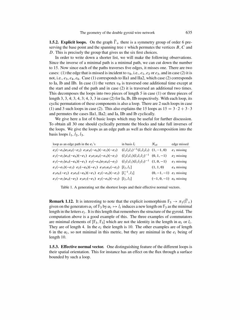
We give here a list of 6 basic loops which may be useful for further discussion.To obtain all 30 one should cyclically permute the blocks and take full inverses ofthe loops. We give the loops as an edge path as well as their decomposition into thebasis loops l1, l2, l3.

loop as an edge path in the ei ’s in basis li Neff edge missed

e2.�e4/e5e6.�e2/ e3e4.�e6/.�e5/.�e3/ .l1l2l3/�1.l1l2l3/ .1; �1; 0/ e1 missing

e1.�e5/e4.�e6/.�e1/ e3e5e6.�e4/.�e3/ .l2l3l1/.l3l1l2/�1 .0; 1; �1/ e2 missing

e1.�e5/e4.�e6/.�e1/ e2.�e4/e5e6.�e2/ .l2l3l1/.l1l2l3/�1 .1; 0; �1/ e3 missing

e1.�e5/.�e3/ e2.�e6/.�e1/ e3e5e6.�e2/ Œl2; l1� .1; 1; 0/ e4 missing

e1e6.�e2/ e3e4.�e6/.�e1/ e2.�e4/.�e3/ Œl�11 ; l3� .0; �1; �1/ e5 missing

e1.�e5/e4.�e2/ e3e5.�e1/ e2.�e4/.�e3/ Œl2; l3� .�1; 0; �1/ e6 missing

Table 1. A generating set the shortest loops and their effective normal vectors.

Remark 1.12. It is interesting to note that the explicit isomorphism F3 ! �1.x�C/given on the generators ˛i of F3 by ˛i 7! li induces a new length on F3 as the minimallength in the letters ei . It is this length that remembers the structure of the gyroid. Thecomputation above is a good example of this. The three examples of commutatorsare minimal elements of ŒF3; F3� which are not the identity in the length in ˛i or li .They are of length 4. In the ei their length is 10. The other examples are of length6 in the ˛i , so not minimal in this metric, but they are minimal in the ei being oflength 10.

1.5.3. Effective normal vector. One distinguishing feature of the different loops istheir spatial orientation. This for instance has an effect on the flux through a surfacebounded by such a loop.


We assume a constant magnetic field. In this case if S is a surface bounding a loopL D ei1 ; : : : ; ein , let fj ´ Pj

kD1eij . Then, by Stokes, we can just integrate over the

surface given by the union of the triangles defined by .fj ; fj C1/, j D 1; : : : ; n�1. IfNj D fj � fj C1 D fj � ej C1 and Neff ´ Pn�1

j D1Nj , then we have for the magneticflux through S

ˆ D“

S

B dS DX

j

1

2B �Nj D 1

2B �Neff

The values for Neff are listed for the basic loops. Notice that inversion of a loopinverts the normal vector, while the cyclic permutation of the components leaves theeffective normal vector invariant.

1.6. Thequantumgraph. In order to promote the skeletal graph to a quantum graph,we will fix a Hilbert space and a Hamiltonian. Here we follow the terminology thata quantum graph is graph with an associated Hilbert space and a Hamiltonian on it.In this paper we will use the generalized Harper Hamiltonian [2], [20].

The original Harper Hamiltonian [12] is obtained for a cubic lattice by using thetight-binding approximation and Peierls substitution for the quasi momentum [16].

In the next section we will give the general theoretical setup for this using graphs,groups and representations. For the gyroid the notions such as graphs and groupshave been introduced above, so that the reader may substitute these in the generaldefinitions below.

2. Graph representations and matrix Harper operators

One idea in studying the noncommutative aspects of a given system is to give a K-theoretic gap labeling for the Hamiltonians. For this one considers an algebra B

generated by the Hamiltonian and the symmetries. If everything is commutative thenthis algebra is basically the C*-algebra of functions on the Brillouin zone/torus. Wewill make these ideas precise using physical and mathematical lattices as definedbelow.

2.1. Graph language. For us a graph or an abstract graph � will be a collectionof vertices V.�/ and a collection of edges E.�/ which run between vertices up tobijections preserving the incidences. Each edge can have two orientations. An edgetogether with an orientation is called an oriented edge. Each oriented edge Ee has astarting vertex s.Ee/ and a target vertex t .Ee/. A graph � is called finite if both V.�/and E.�/ are finite sets.

A graph naturally becomes a topological space if the edges are replaced by inter-vals. This space is called the realization of the graph. In more technical terms thedata above gives a one-dimensional CW-complex and we take the realization of this


complex. When we talk about topological properties of a graph, like its fundamentalgroup, we always mean the topological properties of its realization.

A graph is connected if its realization is connected. This means that one can travelto all vertices from any given vertex along the edges. A tree is a connected graphwhose realization is contractible (i.e., the graph has no loops). A choice of root of atree is simply a choice of a vertex and a rooted tree is a tree together with a choiceof a root. Given a graph � a subgraph � is called a spanning tree if it is a tree andthe vertices of � are all of the vertices of � . To have a spanning tree � needs to beconnected. In this case there are usually several choices of spanning trees. A rootedspanning tree is a spanning tree together with the additional choice of a root.

Proposition 2.1. Let x� be a finite graph and � be a rooted spanning tree. Let v0 bethe root. Then �1.x�/ ´ �1.x�; v0/ D Fn, where Fn is the free group in n variablesand n D jE.x�/j � jE.�/j.

Proof. Consider the graph x�=� obtained by contracting all edges of the subgraph � .This is the graph which only has one vertex v0 and all the edges are loops. The twographs x� and x�=� are homotopy equivalent and hence have the same fundamentalgroup. The graph x�=� embeds into the plane with n punctures with each loop goingaround one puncture. To obtain a compatible embedding of � , one blows up theonly vertex of x�=� into the tree � and both graphs are homotopy equivalent to thepunctured plane. x� is thus homotopy equivalent to the wedge product of n circlesS1. It is well known that the first homotopy group of this space is the free group inn generators.

An embedded graph is a graph � together with an embedding of it realizationinto an Rn. Some properties we discuss depend on such an embedding or are derivedfrom it.

Example 2.2. We have so far considered x�crystalC and x�C as abstract graphs and we

have considered �C both as an abstract as well as an embedded graph. The propertiesof having a certain number of loops at a given point are properties of the abstractgraph, while the proof made use of the embedding. The effective normal vectors areproperties of the embedding of the skeletal graph �C into R3.

2.2. Graph Harper operator

Definition 2.3. A C*-representation �� of a graph � is given by the following data:

� a collection of separable Hilbert spaces Hv , one for each v 2 V.�/;� a collection of isometries UEe W Hs.Ee/ ! Ht.Ee/ for each oriented edge Ee such

that UEeU Ee0 D 1 whenever Ee and Ee0 are the two orientations of the same edge.


Remark 2.4. This construction can also be stated in more categorical terms. It is acertain quiver representation. A finite graph � also generates a groupoid (that is acategory in which all morphisms are invertible) and in this setting a representation isa functor from the groupoid to the category of separable Hilbert spaces.

Definition 2.5. Let �� be a representation of a finite graph x� and write Hx� ´Lv2V.x�/ Hv . Define the graph Harper operator H on Hx� by

H ´X

oriented edges EeUEe;

where we have (ab)used the notationUEe to denote the partial isometry on Hx� inducedby the operator of the same name.

2.3. Matrix actions

2.3.1. General setup. Fix some finite index set I , an index o 2 I , and order on Isuch that o is the smallest element. Fix isomorphic Hilbert spaces Hi ; i 2 I and let�i W Ho ! Hi be fixed choice of isomorphisms. We allow a choice of �o. It mightbe that �o D id but this is not necessary.

Set H D Li2I Hi .

In this situation there is an action of MjI j.End.Ho// on H given as follows. LetA 2 MjI j.End.Ho// be an endomorphism valued matrix. Then the action of A onH is given by

H DMi2I

Hi

˚i ��1i��! H ˚jI j

o

A��! H ˚jI jo

˚i �I��! H :

Vice versa, given an endomorphismH 2 End.H / there is a corresponding matrixM.H/ 2 MjI j.Ho/ given by

H ˚jI jo

˚i �i��! HH��! H

˚i ��1i��! H ˚jI j

o :

That is, if ˆ D Li �i , then M.H/ D ˆ�1 BH Bˆ.

2.3.2. Matrix action for the graph Harper operator. In order to write the Harperoperator of §2.2 as a matrix according to §2.3.1 we need to fix several choices. Wewill assume that the graph � is connected. First there is a choice of base vertex vo

and a choice of order on all vertices in which the base vertex is the smallest. Thenfor each vertex v we choose a fixed path pv – that is, a sequence of ordered edgesEe1; : : : ; Eek – from vo to v. We then set �v ´ �Eek

B � � � B �Ee1W Hvo

! Hv . If v D vo

we also allow the choice �vo´ id W Hvo

! Hvo. This corresponds to the empty

path.


Given such a choice, we obtain the action �p1;:::;pnas above. We call the resulting

matrix the graph Harper operator in matrix form.Given a rooted spanning tree � of � , choose v0 to be the root, and then there is

a unique shortest path on � from v0 to any vertex vi of � , which we can view as apath on � . Thus we get the data needed. Again a convenient choice of paths is givenby a spanning tree. We sometimes write H�;� for the corresponding graph Harperoperator in matrix form.

Remark 2.6. Any two matrix Harper operators are conjugate. This follows simplyby making a base change.

3. C*-geometry of Harper Hamiltonians on lattices

For lattices there are different definitions and connotations in the mathematics andphysics literature. We will use the adjectives “mathematical” and “physical” to dis-tinguish the two. As a reference in the physics literature for the definition of latticeswe use [1].

3.1. Translation action. The additiveAbelian group Rn acts on itself by translation.Write Tw.v/ D v C w. For a subset S 2 Rn and a subgroup L � Rn we denote byL.S/ the set of all translates of points in S under the action of all elements of L.

3.2. Lattices: mathematical, physical and Bravais

Definition 3.1. A mathematical lattice with a basis of rank m in Rn is an injectivegroup homomorphism �L W Zm ,! Rn. If m D n then such a lattice is called aBravais lattice with a basis.

If � is a mathematical lattice with a basis, we letL ´ �L.Zm/ be its image. Thisis a discrete subgroup of Rn, which is isomorphic to Zn. We will refer to L as amathematical/Bravais lattice.

A Bravais subgroup or sublattice is a subgroup L0 � L which is a Bravais lattice.Any Bravais lattice L acts by translations on Rn and a primitive cell is a fundamentaldomain for this action. In general a cell is a fundamental domain for a Bravaissubgroup L0 of L.

Example 3.2. The integer points Zn � Rn are a Bravais lattice, which we call thecrystallographic lattice. A crystallographic cell is a primitive cell for this lattice. Theunit cube is a primitive cell. The cube of length 2 is a cell that is not primitive.

As a definition for a lattice in the physical sense, we will take the followingconvention:


Definition 3.3. A subset ƒ � Rn is a lattice if there is a finite set V � Rn and aBravais lattice L such that ƒ D L.V /.

The tuple .L; V / is called a crystal structure or a lattice with a basis.5 We willnot use the latter terminology as it is mathematically confusing.

Notice that givenƒ neitherL nor V are uniquely defined. We can and will mostlychooseL to be maximal and V to be minimal or primitive. In this case we call .L; V /a primitive crystal structure. Sometimes L is called the space group.

Still there is of course a choice in fundamental domain and hence a choice in V ,but for any two such choices there is a unique bijection. In fact if we let xV be a set oforbits of the L action; then it is unique and any V is just a choice of representatives.It is also easy to see when L is minimal. L is minimal if and only if the number oforbits j xV j is minimal.

3.3. Graphs and lattices. To develop a general theory, we will deal with two cases.The usual case is that given a lattice we obtain a graph by adding edges to the nearestneighbors. But is convenient to also allow that we already have an embedded graph�ƒ whose vertices are the set ƒ. In this case, we will let �ƒ stand for this chosengraph.

3.3.1. Canonical graph of a lattice. Given a lattice ƒ without a pre-chosen graphdefine the graph �ƒ of ƒ to be the graph whose vertices are the elements of ƒ andwhose edges are the line segments between nearest neighbors. This graph is naturallyembedded in Rn and we will sometimes make use of this.

3.3.2. Quotient graphs. Given a choice of symmetry groupL forƒ, we also definethe quotient graph x�ƒ.L/ as �ƒ=L � Rn=L. This is the abstract graph whosevertices are given by xV and whose edges are given by the set of orbits of edges of�ƒ.

If L is a maximal group we will just write x�ƒ.If the unit cell is a cell for L corresponding to a subgroup L0, we also define the

crystallographic quotient graph of ƒ to be the graph x�ƒ.L0/.

3.4. Group of a lattice. A lattice ƒ also generates a discrete subgroup of Rn asfollows: using the natural embedding �ƒ � Rn we can think of any directed edge Eeof �ƒ of �ƒ simply as a vector in Rn. Then there is an associated translation operatorTEe . Notice that as vectors the translates of all the oriented edges correspond to oneanother. This means that the set of vectors Ee is given by one vector in each orbit oforiented edges of the embedded graph �ƒ. This set is in bijection with the orientededges of x�ƒ and we will not distinguish between them in the notation. That is, wewrite Ee for both the oriented edge of the abstract graph x�ƒ and the vector in Rn it is

5Usually one would include labels such as atom labels to V .


in bijection with. We will enumerate the set of vectors fEeg as Eei . These vectors thengive a symmetric group of generators of an Abelian subgroup of Rn, which we callthe lattice group T .ƒ/ of ƒ. It is the group generated by the Eei This group consistsof all elements of the form

T .ƒ/ ´ ˚ Pi ai Eei j ai 2 Z

�:

Proposition 3.4. T .ƒ/ is a mathematical lattice.

Proof. To generate the group we only need one choice of orientation per edge. LetEej , j 2 J , be such a choice. This choice defines a map ZJ ! Rn. The image of thisgroup is a torsion-free Abelian group and hence by the structure theorem for Abeliangroups a free Abelian group of rank � jJ j.

T .ƒ/ also naturally acts by translations on Rn.

3.5. Fundamental group. The graph �ƒ is a covering space for x�ƒ. Since weknow the fundamental group of x�ƒ by Proposition (2.1), this information can beused to calculate the fundamental group of �ƒ. In order to do the computation,we will have to fix some notation. We fix a rooted spanning tree � of x�ƒ and setn ´ jE.x�ƒ/j � jE.�/j. By contracting � we obtain a surjection � W x�ƒ ! ^n

iD1S1,

which by Proposition (2.1) induces an isomorphism on fundamental groups. Wefix generators of �1.^n

1S1/ and choose lifts l1; : : : ; ln of them. By definition each

loop li is a sequence of directed edges Eei1 ; : : : ; Eeik.i/for some k.i/. We set Eli ´

Eei1 C � � � C Eeik.i/.

Proposition 3.5. Letƒ be a lattice with graph �ƒ and finite quotient graph x�ƒ. Let� be a rooted spanning tree for x�ƒ and set n ´ jE.x�ƒ/j � jE.�/j. If the vectors Eliare linearly independent, then �1.�ƒ/ D ŒFn; Fn�. Furthermore a loop on x�ƒ lifts toa loop on �ƒ if and only if it traverses each edge the same number of times in eachdirection.

Proof. We need to compute which loops on x�ƒ lift to loops on �ƒ and which do not.Given a loop l on x�ƒ it can be written as a word in the basis loops li , sayw D Q

j l�.j /ij

where �.j / D ˙1. Fixing a pre-image of v0 given by the rooted spanning tree, thislifts to an edge path on �ƒ given by the sequences of vectors Eei1 ; : : : ; Eeik.i/

. Noticethat l�1

i gives rise to the sequence �Eeik.i/; : : : ;�Eei1 . These vectors form a closed

loop if and only if they all sum up to E0. Now each l˙1i contributes ˙Eli to the sum.

This means that w lifts to a loop if and only ifP

j �.j /Eli D E0. Since by assumption

the Eli are linearly independent, this happens if and only if for fixed i the sum of theexponents of the occurring li is zero, and this happens precisely if the image of w inthe Abelianization Ab.Fn/ ´ Fn=ŒFn; Fn� D Zn is 0. This means that the covering


group of the cover �ƒ ! x�ƒ is Ab.Fn/, which is a normal subgroup of Fn andhence the covering group of �ƒ is ŒFn; Fn�. The last statement follows immediatelyby noticing that this is true for the Eli and hence also for their summands Eeij .

3.6. Main examples

3.6.1. The honeycomb lattice. The honeycomb lattice (see Figure 7) is an exampleof a physical lattice. To make things precise, we letƒhex � R2, which is the Bravaislattice generated by �e1 ´ .1; 0/ and e3 ´ 1

2.1;�p

3/. We set e2 D �e1 � e3 D12.1;

p3/. A “dual” Bravais lattice ƒt

hex generated by f2 ´ e2 � e1 D 12.�3;p3/

and f3 ´ e3 � e1 D 12.3;

p3/ acts via translation onƒhex. There are precisely three

orbits of this action. These are the A, B and C lattices, where we fix the A latticeto be the orbit of .1; 0/, the B lattice to be the orbit of .�1; 0/, and the C lattice tobe the orbit of .0; 0/. The lattice ƒhc is then defined to be the union of the A and Bsublattices. In ƒhc there are three nearest neighbors as indicated in Figure 7.

The symmetry group is Z2 embedded as the “dual” Bravais lattice above. Thegroup T .ƒhc/ is again isomorphic to Z2, but it is the original triangular lattice gen-erated by e1 and e3. See Figure 7. This defines the graph �ƒhc .

A

B

e1

e2

e3

f3

f2

Figure 7. The honeycomb latticeƒhon, the generators fi for L.ƒhon/ and the generators ei ofT .ƒhon/.

3.6.2. The gyroid lattice graph. The gyroid lattice is given by the set of verticesVC of �C of §1. It is also a physical lattice. Here the symmetry group is the spacegroup of I4132, which is the body centered cubic (bcc) lattice. The group T .ƒ/ isactually the face centered cubic (fcc) lattice as shown in Proposition 1.8.

3.7. Hilbert space of a lattice. Given a lattice or in general a countable set ƒ, wedefine its Hilbert space to be Hƒ ´ l2.ƒ/, which is the set of square summable


complex sequences indexed by ƒ. There is an alternative way to think about asequence .a� W 2 ƒ/ as a function on ƒ. Given a sequence as above, thefunction is given by f ./ ´ a�. Vice versa, given the sequence is obtained bysetting a� ´ ./.

Given an action of a groupG onƒ there is an induced action ofG on l2.ƒ/ givenby g ./ ´ .g�1.// for g 2 G and 2 l2.ƒ/.

A standard basis for l2.ƒ/ is given by the functions vl.l0/ D ıl;l 0 .

If ƒ is a lattice then there is a unitary representation of ƒ on H D l2.ƒ/, givenvia the translation operators Tl.vl 0/ D vlCl 0 .

Given a latticeƒ and fixing a translation group L, we can decompose the Hilbertspace Hƒ by breaking it down in terms of the orbits of L. More precisely, labelingeach orbit by a vertex in x� , we obtain the direct sum decomposition

Hƒ DMNv2x�

H Nv; (6)

where Hv D l2.L.v// for any v which represents the class of Nv.

3.8. Partial isometries andprojections. In general we get a representation ofL.ƒ/on Hƒ. Notice that there is in general no representation of T .ƒ/ on Hƒ. We do havea partial action, which is given by partial isometries. If Ee is an edge from v tow in x� ,then it induces an isomorphismVEe W Hw ! Hv simply by settingVEe .l/ D .l�Ee/.This induces a partial isometry on all of H .ƒ/.

Another way to describe this partial isometry is as follows. Consider Hƒ. SinceT .ƒ/ � ƒ, after shifting ƒ so that 0 2 ƒ, we have HT .ƒ/ � Hƒ, and moreoverT .ƒ/ acts on HT .ƒ/ via translation operators TEe . If P is the orthogonal projectionof HT .ƒ/ to Hƒ then VEe D PTEeP . If furthermore Pv is the projection onto Hv �HT .L/, then we can further decompose the action into componentsUw;v

Ee D PvTEePw .

Notice that in principle there could be a directed edge e0 ¤ e with Ee0 D Ee as vectorsin Rn. This happens for e.g. the cube in §1.3.1. In this case there will be morecomponents or super selection sectors to use physics terminology.

3.9. Projective representations. Up to now we have insisted that the translationoperators are a bona fide representation of the translations groups.

It turns out that to accommodate such physical data as a magnetic field one shouldonly expect a projective representation. This is also in accord with general quantumtheory, where representations are always only expected to be projective.

This is also one of the sources of noncommutativity, the second being that onedoes not expect the symmetries of the system to commute with the Hamiltonian on thenose. One actually has a choice either to preserve the commutativity of the symmetryoperators or to preserve that the symmetry operators commute with the Hamiltonian.We recall some standard facts from representation theory.


3.9.1. Cocycles. A U.1/ 2-cocycle for a group G written as c 2 Z2.G;U.1// is amap c W G �G ! U.1/ such that

c.u; v/c.uv;w/ D c.u; vw/c.v; w/;

which is called a cocycle condition.Notice that if c is a U.1/ 2-cocycle for G and H � G is a subgroup, then its

restriction cjH W H �H ! U.1/ is a U.1/ 2-cocycle for H .

Definition 3.6. A morphism � W G ! U.H / is called a projective representationwith cocycle c if �.1G/ D idH , that is, the identity 1G of G maps to the identityoperator idH and �.u/�.v/ D c.u; v/�.uC v/.

Example 3.7. A cocycle c is called trivial if c.u; v/ D s.u/s.v/s�1.uv/ for somegroup morphism s W G ! U.1/. Given a trivial group cocycle one can always perturbor scale an existing representation � to a projective representation �c with cocyclec by setting �c.u/ ´ s.u/�.u/. With the same formula one can scale a projectiverepresentation with a cocycle c0 to one with the cocycle cc0.

Remark 3.8. We will be dealing with Abelian groups G, viz. Zn, for which we willuse the usual additive notation of 0 and C for the identity and group operation.

In the case of a freeAbelian group and its Hilbert space, given any cocycle, one canalso twist the standard representation to a projective representation with that cocycle.

Lemma 3.9. Let L ' Zn � Rn be a lattice and ˛ 2 Z2.L; U.1//. Then theoperators Ul which operate on HL via

Ul.vl 0/ D ˛.l; l 0/vlCl 0 ;

where vl is the standard basis, satisfy

UlUl 0 D ˛.l; l 0/UlCl 0 ; UlUl 0 D �.l; l 0/Ul 0Ul with �.l; l 0/ D ˛.l;l 0/˛.l 0;l/

: (7)

Proof. Straightforward calculation.

Lemma 3.10. Let B be a bilinear form on Rn. Then ˛B.u; v/ ´ ei2 B.u;v/ is a

2-cocycle for Rn. Ifƒ � Rn is a lattice and ei are generators for this lattice, then thealgebra of operators Ul of the ˛ twisted representation is generated by the operatorsUi ´ Uei

.

Proof. First we calculate

˛B.u; v/˛B.uC v;w/ D exp. i2ŒB.u; v/C B.uC v;w/�/

D exp. i2ŒB.u; v/C B.u;w/C B.v;w/�/;

˛B.u; v C w/˛B.v; w/ D exp. i2ŒB.u; v C w/C B.v;w/�/

D exp. i2ŒB.u; v/C B.u;w/C B.v;w/�/:


Secondly, if l D Paiei , then

QU

ai

i / Ul by the formulas (7).

3.9.2. Noncommutative tori. A standard example which will be important in thefollowing is given by the projective action of Zn on H .Zn/ with the cocycle ˛ givenby choosing an anti-symmetric bilinear form B D 2� y‚ on Rn and then restrictingthe cocycle. This yields a cocycle which we call ˛y‚ ´ ˛B.u; v/ D ei� y‚.u;v/.

In this case the operators Ui ´ Ueigenerate the algebra of operators Ul . These

generators satisfy

UiUj D e2�i‚ij TjTi ; ‚ij D y‚.ei ; ej / (8)

This follows from (7); �.Ui ; Uj / D ei�‚ij e�i�‚ji D e2�i‚ij by anti-symmetry of‚. In general:

Definition 3.11. For a fixed anti-symmetric .n� n/-matrix‚ the C*-algebra gener-ated byn unitary operatorsUi on a separable Hilbert space satisfying the commutationrelations (8) is called a noncommutative torus and denoted by T n

‚.

Note that T n ´ T n0 is the commutative C*-algebra corresponding to the torus

T n D .S1/�n under the Gelfand–Naimark theorem.

Example 3.12. n D 2: In this case the skew-symmetric matrix can be writtenas ‚ D

�0 1�1 0

�. And ˛.l; l 0/ D expŒi�.l ^ l 0/�, where for l D .l1; l2/ and

l 0 D .l 01; l 02/: l ^ l 0 ´ det�

l1 l 01

l2 l 02

�and accordingly �.l; l 0/ D e2�l^l 0

. This case is

written as T 2

.

Remark 3.13. As usual, once a basis bi for Rn is fixed, there is a bijection betweenanti-symmetric bilinear forms y‚ and skew-symmetric matrices ‚ given by ‚ij Dy‚.bi ; bj /. If thus choice of basis has been made, we will write˛‚. In our applications,the basis bi will be given to us by a choice of basis for the Bravais lattice L.

3.9.3. Wannier or magnetic translation operators. In case of magnetic field thereis a standard cocycle and representation coming from theB-field. This was first usedin [12]. A magnetic field B in mathematical terms is a 2-form on Rn.

If we assume that theB-field is constant, then this is nothing but a skew-symmetricbilinear form on Rn, thus giving rise to a cocycle ˛B as above. This cocycle can nowbe restricted to any lattice in Rn. Furthermore in this situation, we can choose amagnetic potential A. This is a 1-form on Rn such that dA D B . This form existssince dB D 0, and as Rn is contractible, xH�.Rn/ D 0, i.e., the reduced cohomologyvanishes so that every closed form is exact.

In this case the cocyle is trivial and the twisted action can be rewritten as

Ul 0 .l/ D e�iR .l�l0/

lA .l � l 0/:


Remark 3.14. IfPn

iD1mi D 0 is a closed cycle of vectors bounding a simplyconnected polygonal region D with vertices v1; : : : ; vn such that viC1 D vi C mi ,then Um1

: : : UmnD e�iF id, where F is the flux of B throughD. Furthermore, if B

has a nonsingular vector potential A such that curl.A/ D B , then F D RDBdS DP

i

R 1

0mi � A.vi Cmi t / dt .

This means that given two elements l , l 0 we have

UlUl 0 D �.l; l 0/Ul 0Ul ; �.l; l 0/ D eiR

R BdS ;

where R is the rectangle spanned by the vectors l and l 0.

Example 3.15. In the square lattice, if we choose a constant magnetic field in z-direction EB D Ek orB D 2�dx^dy, then we can chooseA D 1

2.˛1y dxC˛2x dy/

with 2� D ˛2 � ˛1. Setting U ´ Ue1and V D Ue2

we obtain UV D e2�iV U

and this is just ei� where � D RDBdA is the flux through the domain full square A

spanned by e1 and e2. The resulting algebra is T 2

.

3.10. Harper operator for a lattice ƒ and with graph �ƒ. In this section weconstruct a Harper operator for a given latticeƒ and a graph for the lattice �ƒ. Asso-ciated to each such lattice there is a natural separable Hilbert space Hƒ. The Harperoperator is an operator on Hƒ which is obtained by giving a graph representation ofx� . To do this we fix a maximal translational symmetry group L for ƒ (see §3.2).Using the techniques of §2 we obtain a Harper operator as we discuss in detail below.This operator together with the representation of the translation groupL defines a sub-algebra of the endomorphism algebra of Hƒ, which we call the Bellissard–Harperalgebra and denote by B.�ƒ; L; ˛/ or B for short. Here we allow for projectiverepresentations acting with the cocycle ˛, e.g. via a magnetic field (see §3.9.3). If�L, L and ˛ D ˛B with B D 2�i y‚ is fixed, we write By‚ for the correspondingBellissard–Harper algebra.

Furthermore again using §2, we can get a a matrix representation for the Harperoperator and the action of L. These matrices are elements of a matrix algebra withcoefficients in the algebra generated by the operators corresponding toL. Fixing �ƒ,L, a path basis, a basis for L and a magnetic field B D 2� y‚, we arrive at an algebraof matrices, which we call B‚. The details are given below.

3.10.1. Graph representation of x� . To put ourselves in the situation of §2.3.1, wewill decompose Hƒ as

Hƒ DMNv2x�

H Nv;

where Hv D l2.L.v// for any v which represents the class of Nv.We also fix a 2-cocycle ˛B corresponding to a skew-symmetric bilinear form or,

equivalently, a constant B-field. This gives us the Hilbert space part of the data of a


graph representation �x� . We define the isomorphisms as UEe . For this we use the factthat an oriented edge of x� has a natural representation as a vector Ee (see 3.4).

Definition 3.16. The Harper operatorHƒ is defined to be the graph Harper operatorHx� on Hƒ corresponding to the graph representation �� .

The Bellissard–Harper (BH)-algebra B.�ƒ; L; ˛B/ is the C*-algebra of operatorson Hƒ generated by the projective representation ofL and the graph Harper operator.

Remark 3.17. The operator Hƒ also generates random walks and is related to adiscrete difference operator as follows. Let �ƒ be a k-regular graph, which meansthat each vertex has valence k. Then � D k � Hƒ acts as the difference operator.We have �.‰/.l/ D .

PEeWs.Ee/Dl ‰.l/ � ‰.TEe.l///, where the sum is over “nearest

neighbors” as defined by �ƒ.

3.10.2. A matrix representation of the Bellissard–Harper algebra. In order toget a matrix representation, we fix a vertex vo of x�ƒ and a choice of paths pv fromvo to v. We will call such a choice a choice of path basis. Again a convenient way tofix such data is to specify a spanning tree.

We then get a matrix representation of the Harper operator and the operatorscoming from the projective representation of L.

Theorem 3.18. Fixing a choice of path basis and a basis for L, the correspondingfaithful matrix representation of B.�ƒ; L; ˛B/ is a sub-C*-algebra B‚ of the C*-algebraMjV.x�/j.T n

‚/.

Proof. Before passing to the matrix representation, all the operators involved areshifted translation operators, those coming fromL and those coming fromL.ƒ/. Firstwe have to show that the operators fromL still act as operators fromLwhen restrictedto Hvo

, but this is clear since they are diagonal in the direct sum decomposition (6).Thus the operators in question are conjugates, Upv

UlU�

pv/ Ul for any Ul 2 T n

‚.

Here ‚ is the matrix obtained from y‚ D 12�B by using the choice of basis of L.

Secondly, for l 0 2 T .ƒ/, UpvUl 0U �

p0v

/ Ul 00 acts as a translation operator whichpreserves the vo summand. This means that the sum of vectors l 00 D �pv C l 0 � p0

v

is actually in L. Hence the assertion follows.

Notice that different choices of path basis may lead to different representations,but all these representations are isomorphic; moreover they are conjugates of oneanother. The effect of changing the basis ofL is to replace the matrix‚with its basistransform ‚0, but as C*-algebras T n

‚ D T n‚0 – only the presentation has changed –

with the base change acting as an endomorphism.

Corollary 3.19. If ‚ is rational then the spectrum of Hƒ has finitely many gaps.Moreover, the maximal number is determined by the entries of ‚.


Proof. Since there is an injection of B‚ intoMjV.x�/j.T n‚/, we can restrict the tracial

states to B‚. The image of the tracial states of T n‚ is known to be S D Z CP

ij ij Z � R [6], [7]. We fix a faithful tracial state � and then have �.P�/ 2Œ0; jV.x�/j� \ S for any gap projection P�. We thus see that there are only finitelymany possible gaps if all the ij are rational.

3.11. Geometry of B. In general, we are given a lattice ƒ and perhaps the graph�ƒ. We can then obtain a family of BH-algebras by choosing different cocycles˛

2� y‚. We will call an element of this family By‚. Now we have already shown thatsuch an algebra has a faithful matrix representation B‚ � Mk.T

n‚/where k depends

on � . It is interesting to note that this family of subalgebras has different geometriesand K-theories depending on the choice of ‚. Generically one would expect

Expectation 3.20. If ‚ is generic (i.e., all entries are irrational), then B‚ DMjV.x�/j.T n

‚/, which is Morita equivalent to T n‚.

Whether this expectation is met is of course dependent on the choices. It is truefor all the cases we will study. The main motivation is that the noncommutative torusat generic ‚ is simple, i.e., there are no two-sided ideals. This usually allows one tofind that all the elementary matrices are in the algebra and hence the algebra is thefull matrix ring. The details of our particular calculations given in §4 also illuminatethis expectation.

An open question is what happens at non-generic values of‚, i.e., if one or more ofthe entries of‚ are rational. This again heavily depends on the entries ofHƒ. In thecases we study below either B‚ D MjV.x�j.T n

‚/ again, or it is a genuine subalgebra.This is for instance a good new source of such algebras and for families in which theK-theory may jump.

The commutative case B0 is also very interesting. Here we can characterizethe C*-algebra B0 by the space it represents via the Gelfand–Naimark theorem.For this we need some terminology. For each character or C*-algebra morphism� W T n ! C, there is an induced C*-algebra morphism N� W Mk.T

n/ ! Mk.C/ forany k. We fix k D jV.x�/j. We say Hƒ is generic if it has k distinct eigenvaluesin T n or, equivalently, if there is a character � of T n such that N�.H/ has k distincteigenvalues.

We call a point � of T n degenerate if N�.H/ has eigenvalues with higher multiplic-ities. The action of L gives an inclusion i W T n ! B0. Given a character of B0, wealso get a character of T n by pull-back along i . We call a point � of B0 degenerateif i�.�/.H/ has eigenvalues with higher multiplicity.

Theorem 3.21. If Hƒ is generic, then B0 D C �.X/, whereX is a generically k-foldcover of the torus T n. This cover is ramified over the locus of degenerate points andis moreover a quotient of the trivial k-fold cover. Here the identifications are alongdegenerate points of X .


Proof. First observe that the trivial k-fold cover of T n has the C*-algebraT nŒe1; : : : ; ek�=R, where the ei are self-adjoint and generate a semisimple alge-bra. This means that the relations R are equivalent to the equations eiej D ıij ei andPei D 1. Here the ei can be understood as the projectors to each of the copies.Secondly we characterize B0. It is certainly a quotient of the C*-algebra T ŒH �,

where H is a new self-adjoint generator which commutes with the previous gen-erators. The way to understand its quotient is as follows. By the theorem ofCaley–Hamilton we know that the characteristic polynomial p of H annihilates H :p.H/ D 0. We claim this is the only relation. Indeed if there were any other relationr , then we could write r D r 0 C r 00 with r 0 2 .p.H// and r 00 a polynomial in Hof degree less than k. This relation would hold after applying any character �, i.e.,N�.r/ D 0. Since N�.r 0/ D 0 we also get N�.r 00/ D 0. But generically there are k dis-tinct eigenvalues, so that for generic choices of � the minimal polynomial of N�.H/is the characteristic polynomial. Thus, as a polynomial in H , the degree of r 00 mustbe bigger or equal to k, which means that r 00 D 0. Hence B0 D T nŒH �=pŒH�.

We can now give the C*-morphisms corresponding to the geometric continuousmaps: Fk

1 Tn

� ��

�1 ��X

�2��

��

��

T n

Let i 2 T n be the eigenvalues ofH as a matrix with coefficients in the commu-tative ring T n. Then the map � is given by H 7! P

iei . The maps �1 and �2 arejust the inclusion maps. There are sections sk of �1, given by sending ej 7! ıj;k1,which give rise to sections Qsk D � B sk . The corresponding C*-map is given byH 7! k . From this the claims follow readily.

4. Results for the Bravais, honeycomb and gyroid lattices

4.1. The Bravais lattice cases

4.1.1. The Zn case. In case ƒ D Zn, we see that L D T .ƒ/ D Zn and x�ƒ is thegraph with one vertex and n loops.

From the graph x�ƒ we can already read off that �1.�ƒ/ D ŒFn; Fn� accordingto Proposition 3.5, since the condition is obviously satisfied. Minimal loops are oflength 4 and there are

�n2

�unoriented loops.

Fixing a cocycle ˛ by fixing an anti-symmetric matrix‚ (recall that this is equiv-alent to fixing a constant B-field), the corresponding Harper operator is just

HZn DnX

iD1

UeiC U�1

eiD

nXiD1

Ui C U �i ;


where ei are the standard unit basis vectors of Rn and Ui are the generators of thenoncommutative n-torus T n

‚.The algebra generated by the representation ofL D Zn is just the noncommutative

torus T n‚, and since H 2 T n

‚, the algebra B‚ is also the noncommutative torusB‚ D T n

‚.

4.1.2. Other Bravais lattices. Ifƒ is the set of points of a Bravais lattice, then againL D T .ƒ/ D ƒ. For the graph x�ƒ we need the information which of the distancesbetween vertices of ƒ are minimal, or we need the additional data of a graph �ƒ.This information is also crucial in determining �1.

Let ej , j 2 J , be the collection of these minimal vectors and fix an orientation Eejfor each of them. Asƒ D L is a subgroup, 0 2 ƒ, and the minimal vectors are givenby the 2 ƒwith minimal length. Again fix a cocycle ˛ by fixing the anti-symmetricmatrix ‚. Then

Hƒ DXj 2J

UEejC U �

Eej:

The algebra generated by L is always T n‚, and since Hƒ 2 T n

‚, we again obtainB‚ D T n

‚.

Example 4.1. The triangular lattice. This is the lattice spanned by the vectors e1 D.1; 0/ and e2 D .1

2;

p3

2/ in R2. In this case the graph x�ƒ has one vertex and three

loops with the six oriented edges corresponding to ˙e1, ˙e2, ˙.e1 � e2/. Hence thecondition of Proposition 3.5 is not met. One can compute the fundamental group byelementary methods.

The choice of ‚ is given by ‚ D �

0 1�1 0

�. The Harper operator is given by

Hƒtri D Ue1C U �

e1C Ue2

C U �e2

C Ue1�e2C U �

e1�e2

D U1 C U �1 C U2 C U �

2 C U3 C U �3 ;

where U1U2U3 D ei� id. Since H 2 T 2

, the BH-algebra is B‚ D T 2

in thenotation of Example 3.12.

4.2. The honeycomb lattice

4.2.1. Classical geometry. The honeycomb latticeƒ D ƒhon is the two-dimensionallattice specified in §3.6.1. Its quotient graph x�ƒ is the graph with two vertices andthree edges depicted in Figure 8.

We set e1 D .�1; 0/, e2 D 12.1;

p3/ and e3 D 1

2.1;�p

3/. We choose the rootedspanning tree � (root A, sole edge e1 as indicated in Figure 8). The loops ˛ and ˇ liftas l2 D e2.�e1/ and l3 D e3.�e1/. We see that El2 D 1

2.�3;p3/ and El3 D 1

2.3;

p3/.

Thus the condition of Proposition 3.5 is met and we obtain


AA

BB

e1 e2e3

˛ ˇ

Figure 8. The graph x�ƒ for the honeycomb lattice, the spanning tree � (root A, sole edge e1)together with a set of oriented edges, the quotient graph x�ƒ=� .

Proposition 4.2. We have�1.�ƒ/ D ŒF2; F2�:

At each point of the lattice there are six directed or three undirected minimal loopsof length 6.

Proof. It is clear by inspection that there are no loops of length 2 and 4, and the loopsthrough an oriented edge twice will give length bigger than 6. To get a minimal loop,we need to pass through each edge exactly once in each direction, if possible. Thiscan be done by fixing the first edge, and then choosing among the two left over edgesthe second returning edge. Now everything is fixed. One has to leave the vertex bythe last edge and one concludes a cycle of six edges by choosing the only possiblenon-traversed edge oriented without using an oriented edge twice. This of coursegives the known three unoriented loops at each vertex.

Remark 4.3. In the generators ˛, ˇ, these loops are given by the elements Œl2; l3�˙1,Œl�1

2 ; l3�˙1 and Œl2; l�1

3 �˙1.It is interesting to note that the map x�ƒ ! x�ƒ=� induces a new length function

on the free group F2 which is not symmetric in symmetric generators. For instance,the commutator Œl�1

2 ; l�13 � has length 8 in this metric, whereas all other commutators

listed above have length 6 in the generators ei .

Remark 4.4. There is another observation. Given a loop on �ƒ it decomposes intoblocks of loops on x�ƒ. Here we could take the loop l1 D e1.�e2/ e3.�e1/ e2.�e3/

which decomposes into 3 blocks. Now cyclically permuting these blocks, we alsoget a loop on �ƒ, and of course the inverse of any loop is a loop so that the loop l1generates all six loops.

4.2.2. Quantum geometry. Fixing a constant magnetic fieldB D 2� y‚ amounts tochoosing an anti-symmetric bilinear form y‚ on R2. We will use the induced cocycleboth on L and on T .ƒ/. The matrix ‚ is the matrix of y‚ with respect to the basis.f2; f3/ of L. It is completely determined by its value y‚.f2; f3/. The cocycleinduced on T .ƒ/ will also play a role. It is fixed by the value y‚.e1; e2/. We fix the


notation that

´ y‚.f2; f3/; q ´ e2�i and � D y‚.�e1; e2/; � ´ ei�� : (9)

The values of � and are not independent:

D �3� and q D N�6:

This follows from the elementary calculation

D y‚.f2; f3/ D y‚.e2 � e1; e3 � e1/

D y‚.e2; e3/C y‚.e2;�e1/C y‚.�e1; e3/C y‚.�e1;�e1/

D y‚.e2;�e1/ � � C y‚.�e1;�e2/ D �3�:The Hilbert space H D l2.ƒhon/ splits

Hhon D HA ˚ HB ;

where A and B are the vertices as indicated in Figure 8. The six oriented edges ˙ei ,i D 1; : : : 3, of x�ƒ give rise to three partial isometry operators U˙i :

Ui ´�0 0

Uei0

�; U�i ´

�0 U�ei

0 0

�;

where Ueiand U�ei

D U�1ei

D U �ei

are the isomorphisms as in §3.8.The Harper Hamiltonian now reads:

Hƒ D3X

iD1

Ui C U�1i D

�0 U �

e1C U �

e2C U �

e3

Ue1C Ue2

C Ue30

�:

In order to put it into a matrix form with coefficients in T 2

, we again choose thespanning tree � as indicated in Figure 8.

The Hamiltonian now reads

Hƒ;� D�

0 1C U � C V �1C U C V 0

�2 M2.T

2 /;

where we have used the operators U ´ �Uf2and V D N�Uf3

. We have

UV D qV U or UV U � D qV: (10)

The symmetry algebra generated by the translations Ufiis isomorphic to T 2

on

HA ˚ HA. It acts via the representation defined by �.Uf2/ D diag.Uf2

; �2Uf2/ D

diag. N�U; �U / and �.Uf3/ D diag.Uf3

; N�2Uf3/ D diag.�V; N�V /.

Proposition 4.5. If q ¤ ˙1, then B‚ D M2.T 2/ and hence is Morita equivalent

to T 2.


Proof. The strategy of proof is to show that the elementary matrix E12 2 B‚. Ifthis happens, we get that all elementary matrices are in B‚, since E21 D E�

12,E11 D E12E21 and E22 D E21E12 and then B‚ D M2.T 2

/.

The method to obtainE12 is by direct calculation using the commutation relations(10).

The first step is to set X D �. N�2U/�. N�2V �/H�.V /�.U �/ and then set X1 D1

1� Nq ŒH � NqX�. Note we are using the assumption q ¤ 1. Then

X1 D�0 1

1� Nq Œ.1 � N�2/C .1 � N�4/U � C .1 � �4/V �1 0

�:

In step two, we set X2 D H �X1�.1C U C V / D �0 ��0 0

�, where explicitly

�� D BU � C CV � CDU CEV C F U �V CGV �U

with

B D C D �4.1 � �2/

1 � �6; D D 1 � �2

1 � �6; E D N�2. N�2 � 1/

1 � �6;

F D �2.1 � N�4/

1 � �6; G D �2.�4 � 1/

1 � �6:

Notice that �6 D Nq ¤ 1 by assumption. The coefficients do not vanish if �4 ¤ 1 and�2 ¤ 1. But �2 D 1 implies that �6 D 1, and �4 D 1 implies that �12 D 1 and so�6 D q D ˙1. If q ¤ ˙1, then all the coefficients are non-zero. We can obtain E12

in several steps by setting X3 D X2 � �.U /X2�.U�/, X4 D X3 � �.V /X3�.V

�/,X5 D �.U /X4�.U

�/� qX4 and finally obtain E12 D X5 � �. 1. Nq�q/.1� Nq2/

U �V /X5,where for the last step we need the assumption q ¤ �1.

The situation for q D �1 is more complicated. Notice that in this case T 212

is not

simple. For instance, there is a � homomorphism of � W T 212

! Cliff.�Id2/ ˝ C,

where Cliff.�Id2/˝ C is the Clifford algebra over C of the standard quadratic formgiven by the negative of the .2� 2/-identity matrix Id2. If i and j are the usual basisvectors, then �.U / D i , �.V / D j .

We let J ´ ker � D h1C U 2; 1C V 2i.There is also an algebra involution ^ on T 2

12

given by yU D �V , yV D �V .

Proposition 4.6. If q D �1 and �4 ¤ 1, then B‚ D M2.T 212

/. If q D �1 and

�4 D 1, then B‚ is the subalgebra of M2.T 212

/ given by matrices of the form

�a bOb Oa

�C J; a; b 2 T 2

12

; J 2 M2.J/: (11)


Proof. In the case q D �1 we can at first proceed as in the proof of Proposition 4.5.As X1 we obtain

X1 D�0 1

2Œ.1 � N�2/C .1 � �4/.U � C V �/�

1 0

�:

Here the two cases split dependent on whether �4 D 1 or �4 ¤ 1.We will deal with the case �4 ¤ 1 first. We set zX2 D zX1 � �.U / zX1�.�

2U �/,zX3 D zX2 C �.U / zX2�.�

2U �/. Then 1.1�4/.1C4/

zX3 D E21, hence we get E12 DE�

12 2 B‚, and so B‚ is the full matrix algebra.If q D �1 and �4 D 1, then, since q D N�6 D �1, we get N�2 D �1 and

X1 D I D E12 CE21 2 B‚. Furthermore, we get

X2 D�0 1C U � C V � � U � V �1 0

�:

SettingY3 ´ 12�.U /ŒX2C�.U /X2�.�U �/� and zY3 D 1

2�.V /ŒX2��.U /X2�.�U �/

we get

Y3 D�0 1C U 2

0 0

�2 B‚; zY3 D

�0 1C V 2

0 0

�2 B‚:

Let B 0 be the algebra above given in (11). It is easy to check that B 0 is indeeda C*-algebra since M2.J/ is a two-sided ideal of M2.T

212

/ and ^ commutes with �.

Now U � C U and V � C V are both in J so that

H D�

0 1C U � C V �1 � U � � V � 0

�C

�0 0

U C U � C V C V � 0

�2 B 0:

Furthermore certainly the operators of L are in B 0 so that the inclusion B‚ � B 0holds.

On the other hand, sinceL � B‚, all the matrices diag.a; Oa/ are in B‚ and by theabove I 2 B‚ so that all matrices of the form

�a bOb Oa

�are in B‚. Furthermore since the

matrices .1CU 2/E21 and analogously .1CV 2/E21 are in B‚, taking products withI D E12 CE21, we obtain that all the matrices of M2.J/ � B‚. Hence B 0 � B‚,as claimed.

We now analyze the case of q D 1. Let .x/ be the principal (algebra) idealgenerated by x in T 2

0 . Set J1 D .1CU CV /, J2 D .1CU � CV �/ and J12 D J1J2.

Proposition 4.7. If q D 1 and � D ˙1, then B‚ D C �.X/, where X is the doublecover of the torus S1 �S1 ramified at the points .e2�i 1

3 ; e2�i 23 / and .e2�i 1

3 ; e2�i 23 /.

If q D 1 and � ¤ ˙1, then B‚ is equal to the matrix C*-subalgebra of M2.T 20 /

given by matrices in the C*-subalgebra

�.T 2/C�J12 J2

J1 J12

�: (12)


Proof. The first statement follows from Theorem 3.21 for � D 1. The eigenvalues ofH in T 2

0 are ˙p.1C U C V /.1C U � C V �/, which exist by continuous operator

calculus since the operator under the square root is self-adjoint of the form AA� andhence has nonnegative real spectrum. The points of the space X equivalent to B0

where these two eigenvalues coincide are given by precisely the points above.For � D �1, we remark that B‚ D B0, by using the involution U 7! �U ,

V 7! �V .If q D 1, but � ¤ ˙1, we actually know that � is a sixth root of unity and

�2 D 3 D e2�i 13 or �2 D 2

3 , and in these cases �4 D � ¤ 1. Let B 0 be the algebraof (12). Since J �

1 D J2 and both of them are algebra ideals, it is clear that B 0 is aC*-subalgebra. Then it is clear that B‚ � B 0. In order to prove the reverse inclusion,we notice that 1

1�ŒH � �.U /H�2�.U �/� D .1C U C V /E21 2 B‚. Hence also

.1C U � C V �/E21 2 B‚ as well as .1C U C V /.1C U � C V �/E11 2 B‚ and

.1C U C V /.1C U � C V �/E22 2 B‚. This together with the action of L showsthat B 0 � B‚.

In the notation of equation (9):

Theorem 4.8. If q ¤ ˙1, the algebra B‚ has the K0-group Z ˚ Z. If � D ˙1,then K0.B‚/ D Z3.

Proof. For ˛ ¤ 1 this directly follows from Proposition 4.5 below. For the commu-tative case q D 1, � D ˙1, this follows from the fact that the double cover of thetorus obtained by identifying two pairs of points of two tori has the correspondingK0-group.

4.3. The gyroid

4.3.1. The lattice and sublattice Hilbert spaces. The lattice �C has the Hilbertspace H�C

D l2.�C/.The subspace H�C

decomposes naturally into subspaces Hi where Hi D HZ3.vi /

and Z3.vi / denotes the set of all translates under Z3 of vi . Thus H� D L7iD0 Hi .

This is the composition corresponding to x�crystalC . In order to write down the Hamil-

tonian effectively, we will put together the summands in pairs:

H� D HA ˚ HB ˚ HC ˚ HD; (13)

where HA D H0 ˚ H6, HB D H1 ˚ H7, HC D H3 ˚ H5, HD D H2 ˚ H4.This corresponds to passing from x�crystal

C to x�C and to our general setup of graphHamiltonians.


4.3.2. Cocycles for R3. As discussed, choosing a magnetic field corresponds to aprojective representation of �C by unitary operators on H�C

with a cocycle ˛. Werecall this here in a more familiar three-dimensional setting.

A skew-symmetric bilinear form B translates to a more well-known expressionas follows. Let i , j , k be the standard unit vectors on R3, and set Bx D B.j; k/,By D B.k; i/ and Bz D B.i; j /. If EB D .Bx; By ; Bz/, then

B.m;m0/ D EB � .m �m0/; ˛B.m;m0/ D exp.i 1

2EB � .m �m0//:

Indeed ˛B is a cocycle since

B � .m �m0/C B � ..mCm0/ �m00/ D B � .m �m0 Cm �m00 Cm0 �m00/D B � .m � .m0 Cm00//C B � .m0 �m00/:

The physics interpretation of this is that B is a fixed constant magnetic field, andthen ˛B.m;m

0/ is the magnetic flux through the triangle spanned by m an m0.

4.3.3. Cocycles for the gyroid. The maximal translation group L for �C is the bcclattice spanned by the vectors fi given in (2) or gi (3). The lattice group T .�C/is the fcc lattice spanned by the vectors e4, e5, e6. By restricting a cocycle givenby a vector EB on R3, we obtain a cocycle for each of these lattices. Since both thefcc and the bcc lattices are Bravais lattices, these are precisely all cocycles comingfrom cocycles based on anti-symmetric forms y‚ D 1

2�B stemming from a magnetic

field B .We will use the basis .gi / to fix the matrix representation ‚ of y‚.

4.3.4. Graph representation and graph Harper operator on H�C. We fix a vec-

tor B . This fixes the corresponding cocycle ˛.v;w/ ´ ei 12 B �.v�w/. Now consider

the graph representation as defined in §3.10, where the order of the vertices is A, B ,C , D.

Using the fixed cocycle ˛ above, we obtain the partial isometries correspondingto elements of T .�C/. These are Ui ´ Uei

according to the list (4) as discussed in§3.8.

In Hilbert space decomposition (13) the graph Harper operator Hx� becomes the.4 � 4/-matrix

Hx�CD

0BB@0 U �

1 U �2 U �

3

U1 0 U �6 U5

U2 U6 0 U4

U3 U �5 U �

4 0

1CCA :

Recall that Ui D �.ei / and U �i D U�1

i D U�ei.


4.3.5. Matrix Harper operator. We choose the rooted spanning tree � (root A,edges e1, e2, e3) as indicated in Figure 5. Using this we obtain the matrix Harperoperator

Hx�C;� D

0BB@0 1 1 1

1 0 U �1 U

�6 U2 U �

1 U5U3

1 U �2 U6U1 0 U �

2 U4U3

1 U �3 U

�5 U1 U �

3 U�4 U2 0

1CCA μ

0BB@0 1 1 1

1 0 A B�1 A� 0 C

1 B C � 0

1CCA

according to §3.10.2. The coefficients can be expressed in terms of the operators ofthe magnetic translation operators of the bcc lattice. We fix U ´ Uf1

, V ´ Uf2

and W ´ Uf3for the fi listed in (2). Then

A D aV �W; B D bW U �; C D cW �UV;where

a D ˛.e2;�e6/˛.e2 � e6;�e1/

˛.�f2; f3/;

b D ˛.�e3;�e5/˛.�e3 � e5; e1/

˛.f3;�f1/;

c D ˛.�e2; e4/˛.�e2 C e4; e3/

˛.�f3; f1/˛.�f3 C f1; f2/:

4.3.6. Choices and notation. In order to proceed we fix some convenient basis andnotation. First we change from the basis fi to the basis

g1 D �f2 C f3; g2 D �f1 C f3; g3 D f1 C f2 � f3

for the bcc lattice B . We see that A D a0Ug1, B D b0Ug2

; C D c0Ug3again for

fixed constants a0 D ˛.�e1;�e6/˛.�e1 �e6; e2/, b0 D ˛.�e3;�e5/˛.�e3 �e5; e2/

and c0 D �˛.�e2; e4/˛.�e2 C e4; e3/. The operators A, B , C again generate theC*-algebra of the noncommutative torus T 3

‚, where ‚ is the matrix of the bilinearform in the basis gi . Explicitly:

12 D 12�B � .g1 � g2/; 13 D 1

2�B � .g1 � g3/; 23 D 1

2�B � .g2 � g3/:

We write ˛1 ´ e2�i12 D ˛2.g1; g2/, N̨2 ´ e2�i13 D ˛2.g1; g3/ and ˛3 ´e2�i23 D ˛2.g2; g3/. This means for the commutators

AB D ˛1BA; AC D N̨2CA; BC D ˛3CB:

4.3.7. Matrix action of T.�C/. Given the choice of the spanning tree � also deter-mines the action of T .�C/.

It will be convenient to introduce forth roots of the ˛i :

�1 D e�2 i12 ; �2 D e

�2 i31 ; �3 D e

�2 i23 ; ˆ D �1�2�3


and the matrices

ƒ1 D diag.1; �1; �2; �1�2/; ƒ2 D diag.1; �1; �1�3; �3/;

ƒ3 D diag.1; �2�3; �2; �3/:

By definition ˛1˛2˛3 D ˆ4.Then the action � is given by the matrices

�.A/ D ƒ1 diag.A;A;A;A/;

�.B/ D ƒ2 diag.B;B;B;B/;

�.C / D ƒ3 diag.C; C; C; C /:

Note the following which makes the calculations quite a bit simpler:

ƒ1ƒ�2 D diag.1; 1; x̂ ; ˆ/; ƒ2ƒ

�3 D diag.1;ˆ; x̂ ; 1/; ƒ1ƒ

�3 D diag.1;ˆ; 1; x̂ /:

4.3.8. Calculation of B‚ and K�.B‚/

Proposition 4.9. If ˆ ¤ 1, then the BH-algebra B‚ is the full matrix algebraB‚ D M4.T 3

‚/.

Proof. The strategy is to again show that enough elementary matrices are in B‚.This will be done in a case by case study. We will present the first case in detail.

Assume that ˛1 ¤ ˆ2, ˛2 ¤ ˆ and ˛3 ¤ ˆ. Then we have to do six steps toobtain E34. These are

X1 D H � �.AB�/H�.BA�/;X2 D X1 � �.BC �/X1�.CB

�/;X3 D X2 � �.AC �/X2�.CA

�/;X4 D ˆ N̨1X3 � �.AB�/X3�.BA

�/;X5 D x̂˛3X4 � �.BC �/X4�.CB

�/;X6 D ˆ N̨2X5 � �.AC �/X5�.CA

�/:

The resulting matrix is

.1� x̂ 2˛2˛3/.1�ˆ N̨3/.1� x̂˛2/.ˆ N̨1 � x̂ 2˛2˛3/. x̂˛3 �ˆ N̨3/.ˆ N̨2 � x̂˛2/E43;

and the factor is invertible by assumption. This provides E43, E34 D E�43, E33 D

E34E43 and E44 D E43E34. Now to get the other elementary matrices, we first as-sume that�1 ¤ 1. Then setY1 D HE44� N�3�.C /E34,Y2 D �3Y1��.B�/Y1�.B/ D�3. N�1 �1/E24 andE14 D Y1 � N�3�.B/E24, which guarantees that all theEij 2 B‚.If �1 D 1, then we use Z0

2 D N�3Y1 � �.C /H�.C �/ D N�3.1 � ˛3x̂ /E24, so since

˛3 ¤ ˆ, we obtainE24 andE14 (as above) and hence again the whole matrix algebra.


The arguments for the cases ˛1 ¤ ˆ, ˛2 ¤ ˆ2, ˛3 ¤ ˆ and ˛1 ¤ ˆ, ˛2 ¤ ˆ,˛3 ¤ ˆ2 are analogous.

Now by pure logic it follows that B‚ is the full matrix in all cases except the threecases ˛i D ˆ2, j̨ D ˛k D ˆ for fi; j; kg D f1; 2; 3g. We treat only one of thesesince the other two follow symmetrically. So assume that ˛1 D ˆ2, ˛2 D ˛3 D ˆ.In this case the story is similar but faster.

We keepX1,X2 as above. Then ifˆ ¤ x̂ we setX 03 D ˆ��.BC �/X2�.CB

�/ D.1 � ˆ/.1 � x̂ .ˆ � x̂ /E13 and again obtain the full matrix algebra using HE11 toobtain the needed elementary matrices. If ˆ D x̂ , then, since ˆ ¤ 1, we haveˆ D �1, hence ˛2 D ˛3 D �1 and so �2 ¤ N�2 since otherwise �2 D ˙1 and˛2 D �4

2 D 1. Thus we get X 003 D N�2X2 � �.A/X2�.A

�/ D 4. N�2 � �2/E13 withthe factor being invertible. Again we are done.

Proposition 4.10. If ˆ D 1 and not all ˛i D N̨ i D ˙1, then the BH-algebra B‚ isequal to the full matrix algebra B‚ D M4.T 3

‚/.

Proof. As before this follows from an explicit representation of the generators Eij

as expressions in B‚. Since not all ˛i D 1, there must be some ˛i ¤ 1. We willassume that ˛3 ¤ 1. The other calculations are symmetric. Again one has two cases.Either ˛2 D N̨2 or not. In the second case, we set Y1 D H � �.BC �/H�.CB�/ andY2 D ˛2Y1 D �.AC �/Y1�.AB

�/. Put Y3 D ˛3N�1

N�23Y2 � �.C /H�.C �/ and Y4 D

N�1�2Y3��.A/H�.A�/ D .1� N̨3/.˛3� N̨3/.˛3N�2

N�23 � N�2

2�3/. N�1�2�˛2� N�2N�22/E43.

Now as ˛3 ¤ 1: Y4 ¤ 0 if �2 ¤ 1. If �2 D 1, we must have �1 ¤ 1 becauseotherwise �3 would also be 1. In this case, we proceed analogously to obtain E24.In both cases we obtain the full matrix algebra following the strategy used in theprevious proof.

Finally, we deal with the case that ˛2 D N̨2: If ˛2 D 1 then ˛1 D N̨3. It followsthat ˛1 ¤ N̨1, and we are done by an analogous calculation. Indeed, if ˛1 D N̨1 thenalso ˛3 D N̨3 and all ˛i are real, which we excluded.

If ˛2 D �1, then ˛1 D � N̨3. It follows that ˛1 ¤ N̨1, and we are done by ananalogous calculation. If ˛1 D � N̨3, then ˛1 D N̨1 again means that all three ˛i arereal, which was excluded.

Proposition 4.11. If ˆ D 1 and all of the ˛i D 1, then the BH-algebra B‚ is aproper subalgebra of the full matrix algebra B‚ ¨ M4.T 3/.

Proof. We will show this using the character� W T 3 ! C defined by�.A/ D �.B/ D�.C / D 1. This character induces an algebra morphism N� W M4.T 3/ ! M4.C/, andwe will show that N�.B‚/ ¨ M4.C/, which implies the result. We note that

N�.H/ D

0BB@0 1 1 1

1 0 1 1

1 1 0 1

1 1 1 0

1CCA D F � Id with F D

0BB@1 1 1 1

1 1 1 1

1 1 1 1

1 1 1 1

1CCA :


Since ˛i D �4i , all the �i must be fourth roots of unity and furthermore �1�2�3 D 1.

There are again three cases.The first is that all �i D 1. Then N�.�.A// D N�.�.B// D N�.�.C // D Id.

Therefore N�.B‚/ D h N�.H/i � M4.C/. Now F n D 4n�1F and so N�.H/n Did C .

PniD1

�ni

�4i�1/F so that N�.B‚/ is the two-dimensional subalgebra of M4.C/

spanned by Id and F .The second case is that all �2

i D 1 and only one �i D 1. We will assume that�1 D 1, �2 D �1, �3 D �1. The rest of the cases are symmetric.

In this case the image of N� is the 6-dimensional subalgebra of matrices of the form0BB@a b c c

b a c c

d d e f

d d f e

1CCA :

Let B 0 be the subalgebra above. It is an exercise to check that this is indeed asubalgebra. Then N�.�.A// D N�.�.B// D N�.�.C // D diag.1; 1;�1;�1/ so thatN�.B‚/ � B 0. On the other hand, P1 D E11 CE22 D 1

2.Id C diag.1; 1;�1;�1// 2

N�.B‚/ and P2 D E33 C E44 D 12.Id � diag.1; 1;�1;�1// 2 N�.B‚/. And hence

all the Pi N�.H/Pj , i; j D 1; 2, are in N�.B‚/. These are the .2 � 2/ block matricesmaking up N�.H/. But the span of these matrices is precisely B 0.

The final case is that exactly one �2i D 1. We will treat the case �1 D 1, �2 D i ,

�3 D �i . The rest is again symmetric. In this case N�.B‚/ is the 10-dimensionalmatrix algebra of matrices of the form

0BB@a b c d

b a c d

e e g h

f f k l

1CCA :

Let B 00 be the subalgebra above. Again it is an exercise to check that B 00 is in-deed a subalgebra. In the current case we have N�.�.A// D N�.�.B// D N�.�.C // Ddiag.1; 1; i;�i/, so it follows that N�.B‚/� B 00. Now N�.�.A//2 D diag.1; 1;�1;�1/so that P1, P2 above are in N�.B‚/. Furthermore we have �1

2i. N�.�.A//P2 N�.H/P2 �

iP2 N�.H/P2 D E34 and 12i. N�.�.A//P2 N�.H/P2 D iP2 N�.H/P2 D E43, which im-

plies thatE33; E34; E43; E44 2 N�.B‚/. The other generators of B 0 are now given byP1, P1 N�.H/P1, P2 N�.H/P1, E44P2 N�.H/P1, P1 N�.H/P2E33 and P1 N�.H/P2E33,which are all in N�.B‚/.

The trickiest case is the case in which all the ˛i are real and not all equal to 1.

Proposition 4.12. Let ˆ D 1 and let all the ˛i be real, but not all ˛i D 1. If all the�i are different, we either have B‚ D M4.T‚/ or else B‚ ¨ M4.T‚/.


Proof. Since not all ˛i D 1, there must be exactly one ˛i D 1 with the other twobeing equal to �1. We will deal with the case ˛3 D 1, ˛2 D ˛3 D �1. Theothers are similar. Consider X D H C �.BC �/H�.CB�/. Then X2 D 12E11

and X2 D HE11 D E21 C E31 C E41. We know that �1 ¤ �2, �1 ¤ �3 andX3 ´ �1X2 � �.A/X2�.A

�/ D .�1 � �2/E31 C .�1 � �3/E41. Here we get twocases.

If �2 ¤ �3, then we obtain �2X3 � �.A/X3�.A�/ D .�2 � �3/.�1 � �3/E31,

and we have successively E31, E41, E21 and their transposes in B‚. But this is a setof generators.

In case �2 D �3, we see that P1 D 1�1��2

X2 D E31 C E41. Hence alsoE12; E21; E22 2 B‚. Furthermore, P2 D P1E12 D E32 C E42 2 B‚ and Q1 DId �E11 �E22 D E33 CE44 2 B‚, Q2 D Q1HQ1.

We shall use the morphism � W T 3‚ ! Cl ´ Cliff.

�1 00 1

�/˝ C given by �.A/ D

�.B/ D e1, �.C / D e2, where ei , i D 1; 2, are the generators of the Clifford algebrawhich satisfy e2

i D 1 and e1e2 C e2e1 D 1. The map � induces an algebra morphismN� W M4.T 3

‚/ ! Cl.Claim: The image of N� is given matrices of the form0

BB@a b e e

c d f f

g h k l

g h l k

1CCA ;

which is a free rank 10 Cl proper submodule of M4.Cl/ and in turn B‚ is a propersubmodule of M4.T 3

‚/.To prove the claim, we again check both inclusions. Let B 0 be the subalgebra

above. Notice that Id 2 B 0,

N�.H/ D

0BB@0 1 1 1

1 0 e1 e1

1 e1 0 e2

1 e1 e2 0

1CCA 2 B 0;

N��.A/ D N��.B/ D e1 diag.1; �1; �2; �2/ 2 B 0, N��.C / D e2 diag.1; �1; �2; �2/ 2B 0 so that N�.B‚/ � B 0. On the other hand the algebra B 0 is generated byE11, E12,E21, E22, P1, P T

1 , P2, P T2 , Q1, e2 N�.Q2/ D E34 CE43, which are all in N�.B‚/ so

that B‚ � N�.B‚/.

Theorem 4.13. If ˆ ¤ 1 or ˆ D 1 and at least one ˛i ¤ 1 and all �i are different,then B‚ D M4.T 3

‚/ and K.B‚/ D Z4.If �i D 1 for all i , then K.B‚/ D K.X/, where X is the cover of the 3-torus

given by Theorem 3.21.

Proof. The only thing that remains to be proved is that H is generic. Indeed thiscan be done by direct computation. We will not give the eigenvalues here as they are


quite long expressions. But notice that for �.A/ D �1, �.B/ D 1; �.C / D �1 thematrix N�.H/ has the four distinct eigenvalues ˙p

5, ˙1.

Acknowledgments. We would like to thank J. Bellissard, M. Dadarlat, M. Kontse-vich, M. Marcolli and A. Schwarz for enlightening discussions. Foremost, we wish tothank H. W. Hillhouse for sparking the interest in this project and many discussions.

RK thankfully acknowledges support from NSF DMS-0805881 and the HumboldtFoundation. He also thanks the Institut des Hautes Etudes Scientifiques, the Max-Planck-Institute for Mathematics in Bonn and the Institute for Advanced Study fortheir support as well as the University of Hamburg for its hospitality. While at theIAS, RK’s work was supported by the NSF under agreement DMS-0635607.

BK thanks the Department of Physics at Princeton University for its hospitalityand thankfully acknowledges support from the NSF under the grant PHY-0969689.

Any opinions, findings and conclusions or recommendations expressed in thismaterial are those of the authors and do not necessarily reflect the views of theNational Science Foundation.

References

[1] N. W. Ashcroft and N. D. Mermin, Solid state physics. Holt, Rinehart and Winston, NewYork 1976.

[2] J. Bellissard, Gap labelling theorems for Schrödinger operators. In From number theoryto physics (Les Houches, 1989), Springer-Verlag, Berlin 1992, 538–630. Zbl 0833.47056MR 1221111

[3] J. Bellissard, A. van Elst, and H. Schulz-Baldes, The noncommutative geometry ofthe quantum Hall effect. J. Math. Phys. 35 (1994), 5373–5451. Topology and physics.Zbl 0824.46086 MR 1295473

[4] A. L. Carey, K. C. Hannabuss, V. Mathai, and P. McCann, Quantum Hall effect on the hy-perbolic plane. Comm. Math. Phys. 190 (1998), 629–673. Zbl 0916.46057 MR 1600480

[5] A. Connes, Noncommutative geometry. Academic Press, San Diego, CA, 1994.Zbl 0818.46076 MR 1303779

[6] G. A. Elliott, On the K-theory of the C�-algebra generated by a projective representa-tion of a torsion-free discrete abelian group. In Operator algebras and group represen-tations, Vol. I, Monogr. Stud. Math. 17, Pitman, Boston 1984, 157–184. Zbl 0542.46030MR 731772

[7] G.A. Elliott and H. Li, Strong Morita equivalence of higher-dimensional noncommutativetori. II. Math. Ann. 341 (2008), 825–844. Zbl 1153.46045 MR 2407328

[8] K. Grosse–Brauckmann, On gyroid interfaces. J. Colloid Interface Sci. 187 (1997),418–428.

[9] K. Große-Brauckmann and M. Wohlgemuth, The gyroid is embedded and has constantmean curvature companions. Calc. Var. Partial Differential Equations 4 (1996), 499–523.Zbl 0930.53009 MR 1415998

http://www.emis.de/MATH-item?0833.47056

http://www.ams.org/mathscinet-getitem?mr=1221111














[10] D. A. Hajduk, P. E. Harper, S. M. Gruner, C. C. Honeker, G. Kim, E. L. Thomas, andL. J. Fetters, The gyroid: a new equilibrium morphology in weakly segregated diblockcopolymers. Macromolecules 27 (1994), 4063–4075.

[11] T. Hahn (ed.), International tables for crystallography. Vol. A, 5. ed., reprinted withcorrections, Springer-Verlag, Dordrecht 2005.

[12] P. G. Harper, Single band motions of conduction electrons in a uniform magnetic field.Proc. Phys. Soc. A 68 (1955), 874–878.

[13] S. Khlebnikov and H. W. Hillhouse, Electronic structure of double-gyroid nanostructuredsemiconductors: Perspectives for carrier multiplication solar cells. Phys. Rev. B 80 (2009),115316.

[14] C. A. Lambert, L. H. Radzilowski, and E. L. Thomas, Triply periodic level surfaces asmodels for cubic tricontinous block copolymer morphologies. Phil. Trans. R. Soc. Lond.A 354 (1996), 2009–2023.

[15] M. Marcolli andV. Mathai, Towards the fractional quantum Hall effect: a noncommutativegeometry perspective. In Noncommutative geometry and number theory, Aspects Math.E37, Vieweg, Wiesbaden 2006, 235–261. Zbl 1105.81068 MR 2327308

[16] G. Panati, H. Spohn, and S. Teufel, Effective dynamics for Bloch electrons: Peierlssubstitution and beyond. Comm. Math. Phys. 242 (2003), 547–578. Zbl 1058.81020MR 2020280

[17] M. Pimsner and D. Voiculescu, Exact sequences for K-groups and Ext-groups of cer-tain cross-product C�-algebras. J. Operator Theory 4 (1980), 93–118. Zbl 0474.46059MR 587369

[18] M.A. Rieffel,C�-algebras associated with irrational rotations. Pacific J. Math. 93 (1981),415–429. Zbl 0499.46039 MR 623572

[19] M. A. Rieffel and A. Schwarz, Morita equivalence of multidimensional noncommutativetori. Internat. J. Math. 10 (1999), 289–299. Zbl 0968.46060 MR 1687145

[20] T. Sunada, A discrete analogue of periodic magnetic Schrödinger operators. In Geometryof the spectrum (Seattle,WA, 1993), Contemp. Math. 173, Amer. Math. Soc., Providence,RI, 1994, 283–299. Zbl 0805.47028 MR 1298211 (95i:58185)

[21] A. H. Schoen, Infinite periodic minimal surfaces without self-intersections. NASA Tech-nical Note D-5541. Washington, DC, 1970. Zbl 1071.53507

[22] M. F. Schulz, F. S. Bates, K. Almdal, and K. Mortensen, Epitaxial relationship forhexagonal-to-cubic phase transition in a book copolymer mixture. Phys. Rev. Lett. 73(1994), 86–89.

[23] V. N. Urade, T.-C. Wei, M. P. Tate, J. D. Kowalski, and H. W. Hillhouse, Nanofabricationof double-gyroid thin films. Chem. Mater. 19 (2007), 768–777.

Received October 5, 2010

R. M. Kaufmann, Department of Mathematics, Purdue University, 150 N. University Street,West Lafayette, IN 47907-2067, U.S.A.

E-mail: [email protected]












http://www.ams.org/mathscinet-getitem?mr=1298211 (95i:58185)



S. Khlebnikov, Department of Physics, Purdue University, 525 Northwestern Avenue, WestLafayette, IN 47907-2036, U.S.A.


B. Wehefritz–Kaufmann, Department of Mathematics and Department of Physics, 150 N.University Street, Purdue University, West Lafayette, IN 47907-2067, U.S.A.


The geometry of the double gyroid wire network: …ebkaufma/JCommGeom6_12.pdfThe geometry of the...

Documents

Transcript of The geometry of the double gyroid wire network: …ebkaufma/JCommGeom6_12.pdfThe geometry of the...