The Geometry of - Clay Mathematics InstituteAmerican Mathematical Society Clay Mathematics Institute...
202
Transcript of The Geometry of - Clay Mathematics InstituteAmerican Mathematical Society Clay Mathematics Institute...

The Geometry of Algebraic Cycles


American Mathematical SocietyClay Mathematics Institute
Clay Mathematics ProceedingsVolume 9
The Geometry of Algebraic CyclesProceedings of the Conference on Algebraic Cycles, Columbus, Ohio March 25–29, 2008
Reza Akhtar Patrick Brosnan Roy Joshua Editors

2010 Mathematics Subject Classification. Primary 14C15, 14C25, 14C30, 14C35, 14F20,14F42, 19E15.
Library of Congress Cataloging-in-Publication Data
Conference on Algebraic Cycles (2008 : Columbus, Ohio)The geometry of algebraic cycles : proceedings of the Conference on Algebraic Cycles, Colum-
bus, Ohio, March 25–29, 2008 / Reza Akhtar, Patrick Brosnan, Roy Joshua, editors.p. cm. — (Clay mathematics proceedings ; v. 9)
Includes bibliographical references.ISBN 978-0-8218-5191-3 (alk. paper)1. Algebraic cycles—Congresses. 2. Geometry, Algebraic—Congresses. I. Akhtar, Reza, 1973–
II. Brosnan, Patrick, 1968– III. Joshua, Roy, 1956– IV. Title.
QA564.C65685 2008516.3′5—dc22
2010010765
Copying and reprinting. Material in this book may be reproduced by any means for edu-cational and scientific purposes without fee or permission with the exception of reproduction byservices that collect fees for delivery of documents and provided that the customary acknowledg-ment of the source is given. This consent does not extend to other kinds of copying for generaldistribution, for advertising or promotional purposes, or for resale. Requests for permission forcommercial use of material should be addressed to the Acquisitions Department, American Math-ematical Society, 201 Charles Street, Providence, Rhode Island 02904-2294, USA. Requests canalso be made by e-mail to [email protected].
Excluded from these provisions is material in articles for which the author holds copyright. Insuch cases, requests for permission to use or reprint should be addressed directly to the author(s).(Copyright ownership is indicated in the notice in the lower right-hand corner of the first page ofeach article.)
c© 2010 by the Clay Mathematics Institute. All rights reserved.Published by the American Mathematical Society, Providence, RI,
for the Clay Mathematics Institute, Cambridge, MA.Printed in the United States of America.
The Clay Mathematics Institute retains all rightsexcept those granted to the United States Government.
©∞ The paper used in this book is acid-free and falls within the guidelinesestablished to ensure permanence and durability.
Visit the AMS home page at http://www.ams.org/Visit the Clay Mathematics Institute home page at http://www.claymath.org/
10 9 8 7 6 5 4 3 2 1 15 14 13 12 11 10
Contents
Preface vii
Transcendental Aspects 1
The Hodge Theoretic Fundamental Group and its Cohomology 3Donu Arapura
The Real Regulator for a Self-product of a General Surface 23Xi Chen and James D. Lewis
Lipschitz Cocycles and Poincare Duality 33Eric Friedlander and Christian Haesemeyer
On the Motive of a K3 Surface 53Claudio Pedrini
Two Observations about Normal Functions 75Christian Schnell
Positive Characteristics and Arithmetic 81
Autour de la conjecture de Tate a coefficients Z� pour les varietes sur les corpsfinis 83
Jean-Louis Colliot-Thelene et Tamas Szamuely
Regulators via Iterated Integrals (Numerical Computations) 99Herbert Gangl
Zero-Cycles on Algebraic Tori 119Alexander S. Merkurjev
Chow-Kunneth Projectors and �-adic Cohomology 123Andrea Miller
Connections with Mathematical Physics 135
Motives Associated to Sums of Graphs 137Spencer Bloch
Double Shuffle Relations and Renormalization of Multiple Zeta Values 145Li Guo, Sylvie Paycha, Bingyong Xie, and Bin Zhang
v


Preface
The subject of algebraic cycles has its roots in the study of divisors, extendingas far back as the nineteenth century; however, the field truly began to blossomin the mid-twentieth century after Grothendieck’s formulation of a series of conjec-tures which now bear his name. Since then, algebraic cycles have made a significantimpact on many fields of mathematics, among them number theory, algebraic ge-ometry, and mathematical physics, to name only a few. Spencer Bloch introducedthe higher Chow groups in the early 1980s extending the classical Chow-groups androughly having the same relationship to algebraic K-theory as singular cohomologyhas to topological K-theory. The subject has risen to prominence in recent yearsin light of the work of Suslin, Voevodsky, and Friedlander on motivic cohomology,which also identified Bloch’s higher Chow groups with the latter. In particularVoevodsky’s solution of the Milnor conjecture, and work on its extension to otherprimes (the so-called Bloch-Kato conjecture) has stimulated plenty of interest andwork in this area.
Algebraic Cycles II was conceived a sequel to the Conference on Algebraic Cy-cles, held at the Ohio State University in December 2000. The goal of both theseconferences was to stimulate further activity in this area by gathering together ex-perts alongside younger mathematicians beginning work in the field. The scientificprogram of Algebraic Cycles II focused on the study of cycles in the contexts ofarithmetic geometry, motivic cohomology, and mathematical physics. The confer-ence was also held at The Ohio State University, from March 25 to March 29, 2008,and was organized by Reza Akhtar (Miami University), Patrick Brosnan (Univer-sity of British Columbia), Roy Joshua (Ohio State) along with David Ellwood (TheClay Mathematics Institute). The conference featured eighteen 40- or 50- minutetalks and was attended by about 80 participants from all over the world.
It was felt that a volume devoted to the conference proceedings would betterserve the mathematical community. We are very thankful to the Clay MathematicsInstitute for agreeing to publish this volume as part of the Clay MathematicalProceedings (jointly published by the Clay Mathematics Institute and the AmericanMathematical Society). Several of the articles in this volume contain researchpresented at this conference, while others represent separate contributions. Theeditors are happy to acknowledge the enthusiastic support they received from manymathematicians working in this general area, either by contributing a paper to thevolume, by serving as referees or by providing other technical assistance. It is ourhope that this volume will be of value both to established researchers working inthe field and to graduate students who have interest in it.
vii

viii PREFACE
The editors wish to extend their gratitude to the National Security Agency, theNational Science Foundation, the Clay Mathematics Institute, and The Ohio StateUniversity for their financial support of this conference. We recognize in particularDavid Ellwood of the Clay Mathematics Institute for his enthusiasm and supportin agreeing to publish these proceedings. We also wish to thank the excellent tech-nical support we received from Vida Salahi (Clay Mathematics Institute), MarilynRadcliff (Ohio State University), Roshini Joshua (for the Web-page and Poster)and finally everyone else, who helped make this conference a success.
Reza Akhtar, Patrick Brosnan and Roy Joshua
November, 2009

Transcendental Aspects


Clay Mathematics ProceedingsVolume 9, 2010
The Hodge theoretic fundamental group and its cohomology
Donu Arapura
From the work of Morgan [M], we know that the fundamental group of acomplex algebraic variety carries a mixed Hodge structure, which really meansthat a certain linearization of it does. This linearization, called the Malcev or pro-unipotent completion destroys the group completely in some cases; for example ifit were perfect. So a natural question is whether can one give a Hodge structure ona larger chunk of the fundamental group. There have been a couple of approachesto this. Work of Simpson [Si] continued by Kartzarkov, Pantev, Toen [KPT1] hasshown that one has a weak Hodge-like structure (essentially an action by C∗ viewedas a discrete group) on the entire pro-algebraic completion of the fundamental groupwhen the variety is smooth projective. Hain [H2] refining his earlier work [H1], hasshown that a Hodge structure of a more conventional sort exists on the so calledrelative Malcev completions (under appropriate hypotheses). In this paper, I wantto propose a third alternative. I define a quotient of the pro-algebraic completion
called the Hodge theoretic fundamental group πhodge1 (X, x) as the Tannaka dual
to the category local systems underlying admissible variations of mixed Hodgestructures on X, or in more prosaic terms the inverse limit of Zariski closuresof their associated monodromy representations. This carries a nonabelian mixed
Hodge structure in a sense that will be explained below. The group πhodge1 (X, x)
dominates the Malcev completion and the Hodge structures are compatible, and Iexpect a similar statement for the relative completions.
The basic model here comes from arithmetic. Suppose that X is a varietyover a field k with separable closure k. Let X = X ×Spec k Spec k. Suppose thatx ∈ X(k) is a rational point, and that x ∈ X(k) a geometric point lying over it.Then there is an exact sequence of etale fundamental groups
1 → πet1 (X, x) → πet
1 (X, x) → Gal(k/k) → 1
The point x gives a splitting, and so an action of Gal(k/k) on πet1 (X, x). This
action will pass to the Galois cohomology of πet1 (X, x). In the translation into
Hodge theory, πet1 (X, x) is replaced by πhodge
1 (X, x) and the Galois group by a
certain universal Mumford-Tate group MT . The action of MT on πhodge1 (X, x) is
precisely what I mean by a nonabelian mixed Hodge structure. The cohomology
H∗(πhodge1 (X, x), V ) will carry induced mixed Hodge structures for admissible vari-
ations V . In fact there is a canonical morphismH∗(πhodge1 (X, x), V ) → H∗(X,V ). I
Partially supported by NSF.
c© 2010 Donu Arapura
3

4 DONU ARAPURA
call X a Hodge theoretic K(π, 1) if this is an isomorphism for all V . Basic examplesof such spaces are abelian varieties, and smooth affine curves (modulo [HMPT]).I want to add that part of my motivation for this paper is to test out some ideaswhich could be applied to motivic sheaves. So consequently certain constructionsare phrased in more generality than is strictly necessary for the present purposes.
My thanks to Roy Joshua for the invitation to the conference. I would also liketo thank Dick Hain, Tony Pantev, Jon Pridham, and the referee for their comments,and also Hain for informing me of his recent work with Matsumoto, Pearlstein andTerasoma.
1. Review of Tannakian categories
In this section, I will summarize standard material from [DM, D2, D3]. Letk be a field of characteristic zero. Given an affine group scheme G over k, wecan express its coordinate ring as a directed union of finitely generated sub Hopfalgebras O(G) = lim−→Ai. Thus we can, and will, identify G with the pro-algebraic
group lim←−SpecAi and conversely (see [DM, cor. 2.7] for justification).By a tensor category T over k, I will mean a k-linear abelian category with
bilinear tensor product making it into a symmetric monoidal (also called an ACU)category; we also require that the unit object 1 satisfy End(1) = k. T is rigid ifit has duals. The category V ectk of finite dimensional k-vector spaces is the keyexample of a rigid tensor category. A neutral Tannakian category T over k is ak-linear rigid tensor category, which possesses a faithful functor F : T → V ectk,called a fibre functor, preserving all the structure. The Tannaka dual Π(T , F ) ofsuch a category (with specified fibre functor F ) is the group of tensor preservingautomorphisms of F . In more concrete language, an element g ∈ Π(T , F ) con-sists of a collection gV ∈ GL(F (V )), for each V ∈ ObT , satisfying the followingcompatibilities:
(C1) gV⊗U = gV ⊗ gU ,(C2) gV⊕U = gV ⊕ gU ,(C3) the diagram
F (V )gV ��
��
F (V )
��F (U)
gU �� F (U)
commutes for every morphism V → U .
Π = Π(T , F ) is (the group of k-points of) an affine group scheme. Supposethat T is generated, as a tensor category, by an object V i.e. every object of T isfinite sum of subquotients of tensor powers
Tm,n(V ) = V ⊗m ⊗ V ∗⊗n.
Observe that for all m,n ≥ 0
Homk(F (1), F (Tm,n(V ))) = Tm,n(F (V ))
Lemma 1.1. Suppose that T is generated as a tensor category by V , then
(1) Π can be identified with the largest subgroup of GL(F (V )) that fixes alltensors in the subspaces
HomT (1, Tm,n(V )) ⊂ Tm,n(F (V ))
THE HODGE THEORETIC FUNDAMENTAL GROUP AND ITS COHOMOLOGY 5
(2) Π leaves invariant each subspace of Tm,n(F (V )) that corresponds to asubobject of Tm,n(V ).
In particular, Π is an algebraic group.
Proof. This is standard cf. [DM]. �
In general,
Π(T , F ) = lim←−T ′⊂T finitely generated
Aut(F |T ′)
exhibits it as a pro-algebraic group and hence a group scheme.The following key example will explain our choice of notation.
Example 1.2. Let Loc(X) be the category of local systems (i.e. locally constantsheaves) of finite dimensional Q-vector spaces over a connected topological space X.This is a neutral Tannakian category over Q. For each x ∈ X, Fx(L) = Lx givesa fibre functor. The Tannaka dual Π(Loc(X), Fx) is isomorphic to the rationalpro-algebraic completion
π1(X, x)alg = lim←−ρ:π1(X)→GLn(Q)
ρ(π1(X, x))
of π1(X, x).
Given an affine group scheme G, let Rep∞(G) (respectively Rep(G)) be thecategory of (respectively finite dimensional) k-vector spaces on which G acts al-gebraically. When T is a neutral Tannakian category with a fibre functor F , thebasic theorem of Tannaka-Grothendieck is that T is equivalent to Rep(Π(T , F )).The role of a fibre functor is similar to the role of base points for the fundamentalgroup of a connected space. We can compare the groups at two base points bychoosing a path between them. In the case of pair of fiber functors F and F ′, a“path” is given by the tensor isomorphism p ∈ Isom(F, F ′) between these functors.An element p ∈ Isom(F, F ′) determines an isomorphism Π(T , F ) ∼= Π(T , F ′) byg → pgp−1. More canonically, one can define Π(T ) as an “affine group scheme inT ” independent of any choice of F [D2, §6]. For our purposes, we can view Π(T )as the Hopf algebra object which maps to the coordinate ring O(Π(T , F )) for eachF .
Note that Π is contravariant. That is, given a faithful exact tensor functorE : T ′ → T between Tannakian categories, we have an induced homomorphismΠ(T , F ) → Π(T ′, F ◦ E).
2. Enriched local systems
Before giving the definition of the Hodge theoretic fundamental group, it isconvenient to start with some generalities. A theory of enriched local systems E onthe category smooth complex varieties consist of
(E1) an assignment of a neutral Q-linear Tannakian category E(X) to everysmooth variety X,
(E2) a contravariant exact tensor pseudo-functor on the category of smoothvarieties, i.e., a functor f∗ : E(Y ) → E(X) for each morphism f : X → Ytogether with natural isomorphisms for compositions,
(E3) faithful exact tensor functors φ : E(X) → Loc(X) compatible with basechange, i.e., a natural transformation of pseudo-functors E → Loc,

6 DONU ARAPURA
(E4) a δ-functor h• : E(X) → E(pt) with natural isomorphisms φ(hi(L)) ∼=Hi(X,φ(L)). We also require there to be a canonical map p∗h0(L) → Lcorresponding the adjunction map on local systems, where p : X → pt isthe projection.
By a weak theory of enriched local systems, we mean something satisfying(E1)-(E3). We have the following key examples.
Example 2.1. Choosing E = Loc and hi = Hi gives the tautological exampleof a theory enriched of local systems.
Example 2.2. Let E(X) = MHS(X) be the category of admissible varia-tions of mixed Hodge structure [K, SZ] on X. This carries a forgetful functorMHS(X) → Loc(X). Let hi(L) = Hi(X,L) equipped with the mixed Hodgestructure constructed by Saito [Sa1, Sa2]. Here p∗h0(L) is the invariant partLπ1(X) ⊂ L. This can be seen to give a sub variation of MHS by restricting toembedded curves and applying [SZ, 4.19]. Thus MHS(X) is a theory of enrichedlocal systems.
Many more examples of theories of enriched local systems can be obtained bytaking subcategories of the ones above.
Example 2.3. The category E(X) = HS(X) ⊂ MHS(X) of direct sums ofpure variations of Hodge structure of possibly different weights.
Example 2.4. The category E(X) = UMHS(X) ⊂ MHS(X) of unipotentvariations of mixed Hodge structure.
Example 2.5. Finally the category of tame motivic local systems constructedin [A, sect 5] is, for the present, only a weak theory of enriched local systems.However, the category defined by systems of realizations [loc. cit.] can be seen tobe an enriched theory in the full sense.
Given a theory of enriched local systems (E, φ, h•), let φ(E(X)) denote theTannakian subcategory of Loc(X) generated by the image of E(X). So φ(E(X)) isthe full subcategory whose objects are sums of subquotients of objects in the imageof φ. Set πE
1 (X, x) = Π(φ(E(X)), Fx), where Fx is the fibre functor associated toa base point x. More explicitly, this is the inverse limit of the Zariski closures ofmonodromy representations of objects of E(X). It follows that the isomorphismclass of πE
1 (X, x) as a group scheme is independent of x. However, certain additionalstructure will depend on it.
Let κ : E(pt) → E(X) and ψ : E(X) → E(pt) be given by p∗ and i∗ respec-tively, where p : X → pt and i : pt → X are the projection and inclusion of x. Wealso have φ : E(X) → φ(E(X)). These functors yield a diagram
πE1 (X, x) → Π(E(X), x) � Π(E(pt))
where Π(E(X), x) = Π(E(X), Fx) and Π(E(pt)) = Π(E(pt), pt). The diagramis clearly canonical in the sense that a morphism f : (X, x) → (Y, y) of pointedvarieties gives rise to a larger commutative diagram
πE1 (X, x) ��
��
Π(E(X), x)��
��
Π(E(pt))��
=
��πE1 (Y, y)
�� Π(E(Y ), y)��Π(E(pt))��

THE HODGE THEORETIC FUNDAMENTAL GROUP AND ITS COHOMOLOGY 7
Theorem 2.6. The sequence
1 → πE1 (X, x) → Π(E(X), x) � Π(E(pt)) → 1
is split exact. Therefore there is a canonical isomorphism
Π(E(X), x) ∼= Π(E(pt))� πE1 (X, x).
Proof. Since ψ ◦ κ = id, the induced homomorphisms
Π(E(pt)) → Π(E(X), x) → Π(E(pt))
compose to the identity. The injectivity of πE1 (X, x) → Π(E(X), x) follows from
[DM, 2.21].Therefore it remains to check exactness in the middle. An element of
im[πE1 (X, x) → Π(E(X), x)]
is given by a collection of elements gV ∈ GL(φ(V )x), with V ∈ ObE(X), satisfying(C1)-(C3) such that
(1) gU = αx ◦ gV ◦ α−1x
holds for any isomorphism α : φ(V ) ∼= φ(U). While an element of ker[Π(E(X), x) →Π(E(pt))] is given by a collection {gV } such that gV = I for any object in the imageof κ. If V is in the image of κ, the underlying local system is trivial. This impliesthat gV = αx ◦ α−1
x = I, if (1) holds. Thus, we have
im[πE1 (X, x) → Π(E(X), x)] ⊆ ker[Π(E(X), x) → Π(E(pt)]
Conversely, suppose that {gV } is an element of the kernel on the right. Givenan isomorphism α : φ(V ) → φ(U), we have to verify (1). Let H = κ(h0(V ∗ ⊗ U)),then gH = 1 by assumption. H gives a subobject of V ∗ ⊗ U which maps to theinvariant part φ(V ∗ ⊗ U)π1(X) of the local system φ(V ∗ ⊗ U). This follows fromour axiom (E4). Therefore, α gives a section of φ(H). The evaluation morphismev : (V ∗ ⊗ U) ⊗ V → U restricts to give a morphism H ⊗ V → U . We claim thatthe diagram
φ(V )xα⊗I
��
gV
��
α
��φ(H)x ⊗ φ(V )x ev
��
I⊗gV
��
φ(U)x
gU
��φ(V )x
α⊗I ��
α
��φ(H)x ⊗ φ(V )xev �� φ(U)x
commutes. The commutativity of the square on the left is clear. For thecommutativity on right, apply (C1) and (C3) and the fact that gH = I. Equation(1) is now proven. �
Since any representation of an affine group scheme is locally finite, it followsthat Rep∞(E(pt)) can be identified with the category of ind-objects Ind-E(pt).We will often refer to an object of this category as an E-structure. To simplifynotation, we generally will not distinguish between V and φ(V ). By a nonabelianE-structure, we will mean an affine group scheme G over Q with an algebraic actionof Π(E(pt)). Equivalently, O(G) possesses an E-structure compatible with the Hopfalgebra operations. A morphism of nonabelian E-structures is a homomorphismof group schemes commuting with the Π(E(pt))-actions. The previous theoremyields a nonabelian E-structure on πE
1 (X, x) which is functorial in the category of

8 DONU ARAPURA
pointed varieties. When X is connected, for any two base points x1, x2, πE1 (X, x1)
and πE1 (X, x2) are isomorphic as group schemes although the E-structures need not
be the same.
Lemma 2.7. An algebraic group G carries a nonabelian E-structure if and onlyif there exists a finite dimensional E-structure V and an embedding G ⊆ GL(V ),such that G is normalized by the action of Π(E(pt)). A nonabelian E-structure isan inverse limit of algebraic groups with E-structures.
Proof. Suppose that G is an algebraic group with an E-structure. ThenΠ = Π(E(pt)) acts on G; denote this left action by mg. We also have a left actionof Π on O(G), written in the usual way, such that
(2) m(gf) = (mg)(mf)
for m ∈ Π, g ∈ G and f ∈ O(G). This gives an action of Π � G on O(G).Let V ′ ⊂ O(G) be a subspace spanned by a finite set of algebra generators. LetV ⊂ O(G) be the smallest Π�G-submodule containing V ′. By standard arguments,V is finite dimensional and faithful as aG-module. So we getG ⊆ GL(V ). Equation(2) implies that G is normalized by Π. This proves one direction. The converse isclear.
For the second statement write O(G) as direct limit O(G) = lim−→Vi of finite
dimensional E-structures. Let Ai ⊂ O(G) be the smallest Hopf subalgebra contain-ing Vi. This is an E-substructure. So we have G = lim←−Ai which gives the desiredconclusion. �
An E-representation of a nonabelian E-structure G is a representation on anE-structure V such that (2) holds. The adjoint representation gives a canonicalexample of an E-representation. The above lemma says that every finite dimen-sional nonabelian E-structure has a faithful E-representation. The following isstraightforward and was used implicitly already.
Lemma 2.8. There is an equivalence between the tensor category of E-represen-tations of a nonabelian E-structure G and the category of representations of thesemidirect product Π(E(pt))�G.
Corollary 2.9. In the notation of theorem 2.6, E(X) is equivalent to thecategory of finite dimensional E-representations of πE
1 (X, x).
3. Nonabelian Hodge structures
The category MHS = MHS(pt) (respectively HS = HS(pt)) is just the cate-gory of rational graded polarizable rational mixed (respectively pure) Hodge struc-tures [D1]; its Tannaka dual will be called the universal (pure) Mumford-Tategroup and will be denoted by MT (PMT ). The Tannaka dual of the category ofreal Hodge structures R-HS is just Deligne’s torus S = ResC/RC
∗. So the obviousfunctor R-HS → HS⊗R yields an embedding S(R) ↪→ PMT (R). In more concreteterms, (z1, z2) ∈ S(C) = C∗ × C∗ acts by multiplication by zp1 z
q2 on the (p, q) part
of a pure Hodge structure. Since HS is semisimple, PMT is pro-reductive. Theinclusion HS ⊂ MHS gives a homomorphism MT → PMT . We have a sectionPMT → MT induced by the functor V → GrW (V ) = ⊕GrWi (V ). Thus MT is asemidirect product of PMT with ker[MT → PMT ]. The kernel is pro-unipotentsince it acts trivially on W•V for any V ∈ MHS.

THE HODGE THEORETIC FUNDAMENTAL GROUP AND ITS COHOMOLOGY 9
Rep∞(MT ) is the category Ind-MHS of direct limits of mixed Hodge struc-tures. Given an object V = lim−→Vi in this category, we can extend the Hodge andweight filtrations by F pV = lim−→F pVi and WkV = lim−→WkVi.
Set πhodge1 = πE
1 for E = MHS. So this is the inverse limit of Zariski closuresof monodromy representations of variations of mixed Hodge structures. The keydefinition is:
(NH1) A nonabelian mixed (respectively pure) Hodge structure, or simply anNMHS (or an NHS), is an affine group scheme G over Q with an alge-braic action of MT (respectively PMT ).
A morphism of these objects is a homomorphism of group schemes commutingwith theMT -actions. A Hodge representation is anMT -equivariant representation;it is the same thing as an E-representation for E = MHS. The coordinate ring ofan NMHS is a Hopf algebra in Ind-MHS. Let us recapitulate the results of theprevious section in the present setting.
• πhodge1 (X, x) has an NMHS which is functorial in the category of smooth
pointed varieties (and this structure will usually depend on the choice ofx).
• An algebraic group G admits an NMHS if and only if it has a faithfulrepresentation to the general linear group of a mixed Hodge structure forwhich MT normalizes G.
• Admissible variations of MHS correspond to Hodge representations of
πhodge1 (X, x).
The notion of a nonabelian mixed Hodge structure is fairly weak, althoughsufficient for some of the main results of this paper. At this point it is not clearwhat the optimal set of axioms should be. We would like to spell out some further
conditions which will hold in our basic example πhodge1 .
(NH2) An NMHS G satisfies (NH2) or has nonpositive weights if W−1O(G) = 0.
Remark 3.1. To see why this is“nonpositive”, observe that if V is an MHSwith W1V = 0, then W−1O(V ) = W−1Sym
∗(V ∗) = 0. (My thanks to the refereefor pointing out that the weights gets flipped.)
The significance of this condition is explained by the following:
Lemma 3.2. An NMHS G has nonpositive weights if and only if the left andright actions of G on O(G) preserves the weight filtration.
Proof. Note that the left and right G-actions preserves the weight filtrationif and only if
(3) μ∗(WiO(G)) ⊆ O(G)⊗WiO(G)
(4) μ∗(WiO(G)) ⊆ WiO(G)⊗O(G)
Comultiplication μ∗ : O(G) → O(G)⊗O(G) is a morphism of Ind-MHS. If Ghas nonpositive weights, then
μ∗(WiO(G)) ⊆∑j≥0
WjO(G)⊗Wi−jO(G) ⊆ O(G)⊗WiO(G)
(4) follows by symmetry.

10 DONU ARAPURA
Suppose W−1O(G) = 0 and that (3), and (4) hold. Let f ∈ W−1O(G) be anonzero element, and let n > 0 be the largest integer such that f ∈ W−n. Supposethat μ∗(f) =
∑gi ⊗ hi. By (4),∑
gi ⊗ hi ≡ 0 mod O(G)/W−n ⊗O(G)
Therefore all gi ∈ W−n. By a similar argument hi ∈ W−n. Therefore μ∗(f) ∈W−2n(O(G)⊗O(G)). Since morphisms of MHS (and therefore Ind-MHS) strictlypreserve weight filtrations [D1], μ∗(f) = μ∗(f ′) for some f ′ ∈ W−2n. But μ∗ isinjective because μ is dominant. Therefore f = f ′ ∈ W−2n which is a contradiction.
�Lemma 3.3. If G satisfies (NH2), then there is a unique maximal pure quotient
Gpure.
Proof. Since G satisfies (NH2) it acts on the pure Ind-MHS GrW O(G) onthe left. As a group we take Gpure to be the image of G in Aut(GrW O(G)). Toget the finer structure, we apply lemma 2.7, to write G = lim←−Gi with Gi ⊂ GL(Vi)
where Vi ⊂ O(G) are mixed Hodge structures such that Gi is normalized by MT .G preserves W•Vi by assumption. Then
Gpure = lim←− im[Gi → GL(GrW Vi)]
This group carries a nonabelian pure Hodge structure since each group of the limitdoes. By construction, there is a surjective morphism G → Gpure.
Suppose that G → H is another pure quotient. Then G will act on O(H)through this map. The image of G in Aut(O(H)) is precisely H. We have a G-equivariant morphism of Ind-MHSO(H) ⊂ O(G). By purityO(H) = GrW (O(H)) ⊂GrW (O(G)), which shows that theG-action onO(H) factors throughGpure. There-fore the homomorphism G → H also factors through this. �
Before explaining the next condition, we recall that some standard definitions.Fix a real algebraic group G. We have a conjugation g → g on the group ofcomplex points G(C), whose fixed points are exactly G(R). A Cartan involution Cof G is an algebraic involution of G(C) defined over R, such that the group of fixed
points of g → C(g) = C(g) is compact for the classical topology and has a point inevery component. An involution of a pro-algebraic group is Cartan if it descendsto a Cartan involution in the usual sense on a cofinal system of finite dimensionalquotients. Recall that Deligne’s torus S = ResC/RC
∗ embeds into PMT in such away that (z1, z2) ∈ S(C) = C∗×C∗ acts by multiplication by zp1 z
q2 on the (p, q) part
of a pure Hodge structure. It will be convenient to say that a group is reductive(or pro-reductive) when its connected component of the identity is.
(NH3) A NMHS G satisfies (NH3) or is S-polarizable if it has nonpositive weights,and the action C of (i, i) ∈ S(C) on Gpure gives a Cartan involution.
The “S” stands for Simpson, since this condition is related to (and very muchinspired by) the notion of a pure nonabelian Hodge structure introduced by him [Si,p. 61]. Simpson has shown that the pro-reductive completion of the fundamentalgroup of a smooth projective variety carries a pure nonabelian Hodge structure inhis sense. These ideas have been developed further in [KPT1, KPT2]. Althoughthere is no direct relation between these notions of nonabelian Hodge structure,there are a number of close parallels (e.g. lemma 3.7 below holds for both). Themeaning of (NH3) is explained by the following:
THE HODGE THEORETIC FUNDAMENTAL GROUP AND ITS COHOMOLOGY 11
Lemma 3.4. Let G be an algebraic group with an NMHS. Then G is S-polariz-able if and only if there exists a pure Hodge structure V and an embedding Gpure ⊆GL(V ), such that Gpure is normalized by the action of PMT and such that Gpure
preserves a polarization on V . Under these conditions, Gpure is reductive.
Proof. After replacing G by Gpure, we may assume G = Gpure is already pure.Given an embedding G ⊆ GL(V ) as above, choose a G-invariant polarization ( , ) onV . The image W of (i, i) ∈ S(C) in GL(V ) is nothing but the Weil operator for theHodge structure on V . Therefore 〈u, v〉 = (u,W v) is positive definite Hermitian.The group of fixed points under σ(g) = W−1gW is easily seen to preserve 〈 , 〉, soit is compact. In other words, Cg = W−1gW is a Cartan involution. Conversely,if C is a Cartan involution then a G-invariant polarization can be constructed byaveraging an existing polarization over the Zariski dense compact group of σ-fixedpoints. When these conditions are satisfied the reductivity of G follows from theexistence of a Zariski dense compact subgroup. �
Corollary 3.5. The underlying group of a pure S-polarizable nonabelian Hodgestructure is pro-reductive.
Corollary 3.6. If G is S-polarizable, then Gpure = Gred is the maximal pro-reductive quotient of G. In particular, if G is pro-reductive then G = Gpure ispure.
Proof. We have an exact sequence of pro-algebraic groups
1 → U → G → Gpure → 1
where U is simply taken to be the kernel. This can also be described as above by
U = lim←− ker[Gi → GL(GrW Vi)]
We can see from this that U is pro-unipotent. By the previous corollary, Gpure
is pro-reductive. Thus U is the pro-unipotent radical and Gpure = Gred is themaximal pro-reductive quotient. This forces G = Gpure if G is pro-reductive. �
Recall that Simpson [Si, p 46] defined a real algebraic group G to be of Hodgetype if C∗ acts on G(C) such that U(1) preserves the real form and −1 ∈ U(1) actsas a Cartan involution. Such groups are reductive, and also subject to a numberof other restrictions [loc. cit.]. For example, SLn(R) is not of Hodge type whenn ≥ 3.
Lemma 3.7. If an algebraic group admits a pure S-polarizable nonabelian Hodgestructure then it is of Hodge type.
Proof. Choose an embedding G ⊂ GL(V ) as in lemma 3.4. The Hodgestructure on V determines a representation S(C) → GL(VC). The group G(C) isstable under conjugation by elements of PMT (C) ⊃ S(C). Embed C∗ ⊂ S(C)by the diagonal. Then −1 ∈ C∗ acts trivially on G(C). Therefore the C∗ actionfactors through C∗/{±1} ∼= C∗. To see that U(1)/{±1} preserves G(R) ⊂ GL(VR),it suffices to note that the image of eiθ ∈ U(1) in GL(VC), which acts on V pq
by multiplication by e(p−q)iθ, is a real operator. Under the isomorphism U(1) ∼=U(1)/{±1}, −1 on the left corresponds to the image of i on the right. Thus −1acts by a Cartan involution on G(C).
�

12 DONU ARAPURA
Theorem 3.8. Given a smooth variety X, πhodge1 (X, x) carries an S-polar-
izable nonabelian Hodge mixed structure. The category of Hodge representations of
πhodge1 (X, x)red is equivalent to the category of pure variations of Hodge structure
on X.
Proof. For V ∈ MHS(X), let πhodge1 (〈V 〉, x) denote the Zariski closure of the
monodromy representation of π1(X, x) → GL(Vx). Let MT (V ) ⊂ GL(Vx) denotethe Tannaka dual of the sub tensor category of MHS generated by Vx. A slight
modification of theorem 2.6 together with lemma 2.7 shows that πhodge1 (〈V 〉, x) is
normalized by MT (V ). We can also see this directly. The group πhodge1 (〈V 〉, x)
is characterized as the group of automorphisms that fix all monodromy invarianttensors Tm,n(Vx)
π1(X,x). While MT (V ) leaves all sub MHS of Tm,n(Vx) invariant
by lemma 1.1. Let g ∈ MT (V ) and let γ ∈ πhodge1 (〈V 〉, x), then it is enough to
see that g−1γg fixes every tensor in Tm,n(Vx)π1(X,x). This space is a sub MHS of
Tm,n(Vx) by [SZ, 4.19]. Therefore Tm,n(Vx)π1(X,x) is invariant under g (although
it need not fix elements pointwise). This shows that g−1γg fixes the elements of
this space as claimed. Therefore πhodge1 (〈V 〉, x) carries a NMHS.
Since the weight filtration of V is a filtration by local systems, πhodge1 (〈V 〉, x)
preserves W•Vx. So it satisfies (NH2) by lemma 3.2. Let πhodge1 (V ) be the image
of πhodge1 (〈V 〉, x) in GL(GrW Vx). This can be identified with the Zariski closure
of the monodromy representation of the pure variation of Hodge structure GrWV .This pure variation is polarizable by definition of admissibility [SZ, K]. Therefore
GrW Vx possesses a πhodge1 (V ) invariant polarization. Consequently πhodge
1 (〈V 〉, x)satisfies (NH3) by lemma 3.4. Moreover πhodge
1 (V ) = πhodge1 (〈V 〉, x)red is the Tan-
naka dual to the subcategory of Loc(X) generated by the local system GrW V .Putting this all together, we see that
πhodge1 (X, x) = lim←−
V
πhodge1 (〈V 〉, x)
satisfies (NH3), and that the Tannaka dual to HS(X) is PMT � πhodge1 (X, x)red.
Lemma 2.8 implies that HS(X) is equivalent to the category of Hodge representa-
tions of πhodge1 (X, x)red. �
4. Nonabelian variations
The goal of this section is to give a characterization of πhodge1 (X, x). To this
end, we introduce the category of nonabelian variation of mixed Hodge structuresover X, by which we mean the opposite of the category of Hopf algebras in Ind-MHS(X). Given such a Hopf algebra A, we denote the corresponding nonabelianvariation by the symbol SpecA. For any x ∈ X, SpecAx can be understood in theusual sense, and this is an NMHS. Basic examples are given as follows.
Example 4.1. Any object V ∈ MHS(X) can be identified with the nonabelianvariation Spec (Sym∗(V ∗)).
By applying the forgetful functor MHS(X) → Loc(X), we can see that anynonabelian variation SpecA carries a monodromy action of π1(X, x) → Aut(Gx),where Gx = SpecAx. A nonabelian variation of mixed Hodge structures will becalled inner if the monodromy action lifts to a homomorphism π1(X, x) → Gx. The

THE HODGE THEORETIC FUNDAMENTAL GROUP AND ITS COHOMOLOGY 13
examples of 4.1 are rarely inner. However, an ample supply of such examples isgiven by the following.
Example 4.2. For V ∈ MHS(X), we have a nonabelian variation πhodge1 (〈V 〉)
whose fibres are πhodge1 (〈V 〉, x) by [D2, §6]. To construct this directly, note that we
can realize the coordinate ring of πhodge1 (〈V 〉, x) as a quotient of O(GL(Vx)) by a
Hopf ideal∑
fkO(GL(Vx)). The generators fk can be regarded as sections of
R =⊕i,j≥0
Symi(V ∗)⊗ det(V ∗)−j
Thus we can define πhodge1 (〈V 〉) as Spec of the Ind-MHS(X) Hopf algebra
R/(∑
k fkR). This is inner since the monodromy is given by homomorphism
π1(X, x) → πhodge1 (〈V 〉, x).
Let πhodge1 (X) be the inverse limit of πhodge
1 (〈V 〉) over V ∈ MHS(X). The
fibres are πhodge1 (X, x). This is the universal inner nonabelian variation in the
following sense:
Proposition 4.3. If G is an inner nonabelian variation of mixed Hodge struc-ture over X, with monodromy given by a homomorphism ρ : π1(X, x) → Gx. Then
ρ extends to a morphism πhodge1 (X) → G of nonabelian variations.
Proof. Let G = SpecA. Since A ∈ Ind-MHS(X), πhodge1 (X, x) will act on it.
By an argument similar to the proof of lemma 2.7, we can write A as a direct limit
of finitely generated Hopf algebras with πhodge1 (X, x)-action. So that Gx becomes
an inverse limit of algebraic groups carrying inner nonabelian variations. Thus wecan assume that Gx is an algebraic group. By standard techniques we can finda finite dimensional faithful (left) G-submodule V ⊂ O(G). After replacing this
with the span of the πhodge1 (X, x)-orbit, we can assume that V is stable under
πhodge1 (X, x). Therefore V corresponds to a variation of mixed Hodge structure.
By assumption, the image of π1(X, x) in GL(Vx) lies in G. This implies that G
contains πhodge1 (〈V 〉, x) and that ρ factors through it. �
5. Unipotent and Relative Completion
Morgan [M] and Hain [H1] have shown that the pro-unipotent completion ofthe fundamental group of a smooth variety carries a mixed Hodge structure. Wewant to compare this with our nonabelian Hodge structure. We start by recallingsome standard facts from group theory (c.f. [HZ], [Q, appendix A]). Fix a finitelygenerated group π. Then
(a) Q[π], and its quotients by powers of the augmentation ideal J , carry Hopfalgebra structures with comultiplication Δ(g) = g ⊗ g mod Jr.
(b) A finite dimensional Q[π]-module is unipotent if and only if it factorsthrough some power of J . (The smallest power will be called the index ofunipotency).
(c) The set of group-like elements
Gr(π) = {f ∈ Q[π]/Jr+1 | Δ(f) = f ⊗ f, f ≡ 1 mod J}forms a group under multiplication. This is a unipotent algebraic group.

14 DONU ARAPURA
(d) The Lie algebra of Gr(π) can be identified with the Lie algebra of primitiveelements
Gr(π) = {f ∈ Q[π]/Jr+1 | Δ(f) = f ⊗ 1 + 1⊗ f}with bracket given by commutator.
(e) The exponential map gives a bijection of sets Gr(π) ∼= Gr(π). The Lie al-gebra and group structures determine each other via the Baker-Campbell-Hausdorff formula.
(f) Q[π]/Jr+1 is isomorphic to a quotient of the universal enveloping algebraof Gr(π) by a power of its augmentation ideal.
Let ULoc(X) (UrLoc(X)) denote the category of local systems with unipo-tent monodromy (with index of unipotency at most r). The category UrLoc(X)can be identified with the category of Q[π1(X, x)]/Jr+1-modules. We note thatthis category has a tensor product: Q[π1(X, x)]/Jr+1 acts on the usual tensorproduct of representations U ⊗Q V through Δ. With this structure, the categoryof Q[π1(X, x)]/Jr+1-modules is Tannakian. Its Tannaka dual π1(X, x)unr is iso-morphic to the group Gr(π1(X, x)) above, and the Tannaka dual π1(X, x)un ofULoc(X), is the inverse limit of these groups.
We need to impose Hodge structures on these objects.
Lemma 5.1. There is a bijection between
(1) The set of nonabelian mixed Hodge structures on Gr(π).(2) The set of mixed Hodge structures on Gr(π) compatible with Lie bracket.(3) The set of mixed Hodge structures on Q[π]/Jr+1 compatible with the Hopf
algebra structure.
Proof. To go from (1) to (2), observe that a nonabelian mixed Hodge struc-ture always induces a mixed Hodge structure on its Lie algebra compatible withbracket. A Lie compatible mixed Hodge structure on Gr(π) induces an Ind-MHS onits universal enveloping algebra, compatible with the Hopf algebra structure. Thisdescends to Q[π]/Jr+1 by (f) above. A Hopf compatible mixed Hodge structure onQ[π]/Jr+1 induces one on Gr(π) by restriction. �
Hain [H1] constructed a mixed Hodge structure on the Hopf algebra
Q[π1(X, x)]/Jr+1
which is equivalent (in the sense of the lemma) to the one constructed by Morganon Gr(π1(X, x)). These fit together to form an inverse system as r increases. Inbrief outline, Chen had shown that C⊗ lim←−Q[π1(X, x)]/Jr+1 can be realized as the
zeroth cohomology H0(B(x, E•(X), x)) of a complex built from the C∞ de Rhamcomplex via the bar construction:
B•(x, E∗(X), x) = (E∗(X))⊗−•
±dB(α1 ⊗ . . .⊗ αn) = ix(α1)α2 ⊗ . . .⊗ αn
+∑
(−1)iα1 ⊗ . . .⊗ αi ∧ αi+1 ⊗ . . . αn
+(−1)nix(αn)α1 ⊗ . . .⊗ αn−1
±dα1 ⊗ α2 ⊗ . . .⊗ αn
+ . . .

THE HODGE THEORETIC FUNDAMENTAL GROUP AND ITS COHOMOLOGY 15
where ix : E∗(X) → C is the augmentation given by evaluation at x. Hain showedhow to extend B(x, E•(X), x) to a cohomological mixed Hodge complex (or moreprecisely a direct limit of such), and was thus able to deduce the correspondingstructure on cohomology. One thing that is more readily apparent in Hain’s ap-proach is the dependence on base points. As x varies, Q[π1(X, x)]/Jr+1 forms partof an admissible variation of mixed Hodge structure over X called the tautologicalvariation. This is nontrivial since the monodromy representation is the naturalconjugation homomorphism π1(X, x) → Aut(Q[π1(X, x)]/Jr+1).
Wojtkowiak [W] gave a more algebro-geometric interpretation of Hain’s con-struction, which will be briefly described. Bousfield and Kan defined the total spacefunctor Tot [BK, chap X §3], which is a kind of geometric realization, from thecategory of cosimplicial spaces to the category of spaces. The image of the map ofcosimplicial schemes
XΔ[1]=
π
��
X ×X����
��
X ×X ×X��
��
. . .
X∂Δ[1]=
X ×X���� X ×X�� . . .
under this functor is the path space fibration X [0,1] → X{0,1} = X × X. Thehorizontal maps on the top are diagonals (from left to right) or projections (fromright to left); on the bottom they are all identities. The total space of the fibreπ−1(x, x) is the space of loops of X based at x, which is an H-space. There-fore H0(Tot(π−1(x, x)),Q) is naturally a Hopf algebra. This Hopf algebra, whichis described more precisely in [W], can be identified with the coordinate ring oflim←−Gr(π1(X, x)), or Gr(π1(X, x)) if we truncate the cosimplicial space at the rth
stage. This follows from the fact H0(Tot(π−1(x, x)),C) can be computed using thetotal complex of the de Rham complex of the cosimplicial fibre, which is none otherthan B(x, E•(X), x). Under this identification the filtration by truncations inducedon H0 coincides with the filtration by length of tensors on B. The mixed Hodgestructure on H0(Tot(π−1(x, x)),Q) can now be constructed using standard machin-ery: take compatible multiplicative mixed Hodge complexes on each component ofthe cosimplicial space and then form the total complex [W, §5]. Furthermore thetautological variations are given by the 0th total direct images of Q under π|Xunder the diagonal embedding X ⊂ X ×X. A useful consequence of this point ofview is that the MHS on Q[π1(X, x)]/Jr+1 can be seen to come from a motive inNori’s sense [C].
Let UMHS(X) (UrMHS(X)) denote the subcategory of unipotent admissiblevariations of mixed Hodge structure (with index of unipotency at most r). Thetautological variation associated to Q[π1(X, x)]/Jr+1 lies in UrMHS(X). Givenan object V in UrMHS(X), the monodromy representation extends to an algebrahomomorphism
Q[π1(X, x)]/Jr+1 → End(Vx)
which is compatible with mixed Hodge structures.
Theorem 5.2 (Hain-Zucker [HZ]). The above map gives an equivalence be-tween UrMHS(X) and the category of Hodge representations of Q[π1(X, x)]/Jr+1.
The above equivalence respects the tensor structure.

16 DONU ARAPURA
We note that every object of UrLoc(X) is a sum of subquotients of the local sys-tem associated to the tautological representation π1(X, x) → Aut(Q[π1(X, x)]/Jr+1).Therefore φ(UrMHS(X)) = UrLoc(X), where φ : UrMHS(X) → Loc(X) is theforgetful functor. Consequently, we get a split exact sequence
1 �� π1(X, x)unr �� Π(UrMHS(X)) �� MT�� �� 1
by theorem 2.6. In particular, π1(X, x)unr carries an NMHS which is a quotient of
the one on πhodge1 (X, x).
Proposition 5.3. The above NMHS on π1(X, x)unr is equivalent to the Morgan-Hain structure on Q[π1(X, x)]/Jr+1.
Proof. By lemma 5.1, the Morgan-Hain structure on Q[π1(X, x)]/Jr+1 in-duces an NMHS on π1(X, x)unr . Let MH denote the semidirect product of MTwith this Hodge structure on π1(X, x)unr . By theorem 5.2, we have a commutativediagram
UrLoc(X)
=
��
UrMHS(X)φ�� ψ ��
∼=��
MHSκ
��
=
��Rep(π1(X)unr) Rep(MH)�� �� Rep(MT )��
where the functors ψ and κ are given by the fibre and the pullback along theconstant map. Therefore MH is isomorphic to Π(UrMHS(X)) as a semidirectproduct.
�Corollary 5.4. The Morgan-Hain NMHS on π1(X, x)un is a quotient of
πhodge1 (X, x).
Hain has extended the above construction in [H2]. Given a representationρ : π1(X, x) → S to a reductive algebraic group, the relative Malcev completion isthe universal extension
1 → U → G → S → 1
of S by a prounipotent group with a homomorphism π1(X, x) → G such that
π1(X, x) ��
ρ
����������� G
��S
commutes. When ρ : π1(X, x) → S = Aut(Vx, 〈, 〉) is the monodromy represen-tation of a variation of Hodge structure with Zariski dense image, Hain [H2] hasshown that the relative Malcev completion carries a NMHS.
Conjecture 5.5. The relative completion should carry an NMHS in generalwith S equal to the Zariski closure of π1(X, x) → Aut(Vx, 〈, 〉). This should be a
quotient of πhodge1 (X, x).
I am quite confident about this. The essential point would construct an innernonabelian variation of mixed Hodge structure on the family of G as the base point
varies. Then proposition 4.3 would give a homomorphism πhodge1 (X, x) → G. The
main step would be to establish an appropriate refinement of [H2, cor 13.11], and I

THE HODGE THEORETIC FUNDAMENTAL GROUP AND ITS COHOMOLOGY 17
understand that Hain, Matsumoto, Pearlstein, and Terasoma [HMPT] have donethis. J. Pridham has pointed to me that his preprint [P] may also have some bearingon this conjecture.
Remark 5.6. For the applications given later in section 7, only this weaker
statement on the existence of a morphism πhodge1 (X, x) → G extending ρ is needed.
There is one notable case in which this can be deduced immediately. If π1(X, x)is abelian, then G is necessarily abelian, so it splits into a product U × S. Mor-
phisms πhodge1 (X, x) → U and πhodge
1 (X, x) → S can be constructed directly frompropositions 5.3 and 4.3.
6. Cohomology
Fix a theory of enriched local systems E. Let G be a nonabelian E-structure.The category of representations of Π(E(pt)) � G is equivalent to the category ofE-representations of G. Given such a representation V , let H0(G, V ) = V G andH0(Π(E(pt))�G, V ) = V Π(E(pt))�G be the subspaces of invariants. The action ofΠ(E(pt)) on V descends to an action on H0(G, V ). These are left exact functorson the category of representations of Rep∞(Π(E(pt))�G). Since this category hasenough injectives (c.f. [J, I 3.9]), we can define higher derived functorsHi(G, V ) andHi(Π(E(pt)�G, V ). Note that Hi(G, V ) is an E-structure since it is derived froma functor from Rep∞(Π(E(pt) � G) → Rep∞(Π(E(pt)). Alternatively, Hi(G, V )can be computed as the cohomology of a bar or Hochschild complex C•(G, V )[J, I 4.14], which is a complex in Rep∞(Π(E(pt)). We can define cohomology ofΠ(E(pt)) by taking G trivial. We observe that these functors are covariant in Vand contravariant in G.
There are products
Hi(G, V )⊗Hj(G, V ′) → Hi+j(G, V ⊗ V ′)
compatible with E-structures. These can be constructed by either using standardformulas for products on the complexes C•(G,−), or by identifying Hi(G, V ) =Exti(Q, V ) and using the Yoneda pairing
Exti(Q, V )⊗ Extj(Q, V ′) → Exti(Q, V )⊗ Extj(V, V ⊗ V ′) → Exti+j(Q, V ⊗ V ′)
Lemma 6.1. Given an E-representation V of G, Hi(G, V ) = lim−→Hi(G/Hj , VHj )
where Hj runs over all normal subgroups stable under Π(E(pt)) such that G/Hj isfinite dimensional.
Proof. By lemma 3.4 G = lim←−G/Hj is an inverse limit of algebraic groups
with nonabelian E-structures. Clearly V = lim−→V Hj and so
H0(G, V ) = lim−→H0(G/Hj , VHj )
The lemma follows from exactness of direct limits. �
Lemma 6.2. Fix a Hodge representation V of an NMHS G, and an Ind-MHSU . Then
(1) Hi(MT,U) = 0 for i > 1.(2) We have an exact sequence
0 → H1(MT,Hi−1(G, V )) → Hi(MT �G, V ) → H0(MT,Hi(G, V )) → 0

18 DONU ARAPURA
Proof. Write U as a direct limit of finite dimensional Hodge structures Uj ,then
Hi(MT,U) = lim−→Hi(MT,Uj) = lim−→ExtiMHS(Q, Uj)
Beilinson [B] shows that the higher Ext’s vanish, which implies the first statement.For the second statement, note that we can construct a Hochschild-Serre spec-
tral sequence
Epq2 = Hp(MT,Hq(G, V )) ⇒ Hp+q(MT �G, V )
in the usual way. This reduces to the given exact sequence thanks to (1). �
Lemma 6.3. Let G be a nonabelian E-structure and V an E-representation. IfG is pro-reductive then Hi(G, V ) = 0 for i > 0. In general
Hi(G, V ) = H0(Gred, Hi(U, V ))
where U is the pro-unipotent radical and Gred = G/U .
Proof. When G is pro-reductive, its category of representations is semisimple.Therefore H0(G,−) is exact. So higher cohomology must vanish.
In general, the Hochschild-Serre spectral sequence
Epq2 = Hp(Gred, Hq(U, V )) ⇒ Hp+q(G, V )
will collapse to yield the above isomorphism. �
Proposition 6.4. Let X be a smooth variety. Then for each object V ∈ E(X):
(1) Hi(πE1 (X, x), V ) carries a canonical E-structure.
(2) There is natural morphism Hi(πE1 (X, x), V ) → Hi(X,V ) of E-structures.
(3) There are Q-linear maps
Hi(πE1 (X, x), V ) → Hi(π1(X, x), V ) → Hi(X,V )
whose composition is the map given in (2).
Proof. Hi(πE1 (X, x), V ) carries an E-structure by the discussion preceding
lemma 6.1. Note that H0(πE1 (X, x), V ) = V
πE1 (X)
x is nothing but the monodromyinvariant part of Vx, and Hi(πE
1 (X, x), V ) is the universal δ-functor extending it,in the sense of [G]. By axiom (E4), Hi(X,V ) with its E-structure also forms aδ-functor, and there is an isomorphism
H0(πE1 (X, x), V ) ∼= H0(X,V )
of E-structures. Therefore (2) is a consequence of universality.After disregarding E-structure, we can view Hi(πE
1 (X, x), V ) as a universalδ-functor from E(X) → V ectQ. Therefore, from the isomorphisms
H0(πE1 (X, x), V ) ∼= H0(π1(X, x), V ) ∼= H0(X,V ),
we deduce Q-linear maps
Hi(X,V ) ← Hi(πE1 (X, x), V ) → Hi(π1(X, x), V )
The leftmost map was the one constructed in the previous paragraph. Since groupcohomology is also a universal δ-functor from the category of Q[π1(X, x)]-modules

THE HODGE THEORETIC FUNDAMENTAL GROUP AND ITS COHOMOLOGY 19
to V ectQ, we can complete this to a commutative triangle
Hi(πE1 , V ) ��
��
Hi(π, V )
��� ��
��
Hi(X,V )
�
7. Hodge theoretic K(π, 1)’s
The map
(*) Hi(πE1 (X, x), V ) → Hi(X,V )
constructed in the previous section is trivially an isomorphism for i = 0, but usuallynot in general. For instance if i = 2, V = Q and X = P1, the cohomology groupsare 0 on the left and Q on the right.
Let us say thatX is aK(πE, 1) (or a Hodge theoreticK(π, 1) when E = MHS)if (*) is an isomorphism for every V ∈ E(X). When X is a K(π, 1) in the usualsense, then it is a K(πE , 1) if and only if
(**) Hi(πE1 (X, x), V ) → Hi(π1(X, x), V )
is an isomorphism for all V ∈ E(X). The following is a straight forward modifica-tion of [Se, p 13, ex 1].
Lemma 7.1. The following are equivalent
(1) (*) is an isomorphism for all i ≤ n and injective for i = n + 1 for allV ∈Ind-E(X).
(2) (*) is an isomorphism for all i ≤ n and injective for i = n + 1 for allV ∈ E(X).
(3) (*) is surjective for all i ≤ n and all V ∈ E(X).(4) (*) is surjective for all i ≤ n and all V ∈ Ind-E(X).(5) For all V ∈ Ind-E(X), 1 ≤ i ≤ n, and α ∈ H i(X,V ), there exists V ′ ∈
Ind-E(X) containing V such that the image of α in Hi(X,V ′) vanishes.
In particular, X is a K(πE , 1) if (*) is surjective for all i and V ∈ E(X).
Proof. The implications (1)⇒(2) and (2) ⇒(3) are clear. For (3)⇒(4), we canuse the fact that cohomology commutes with filtered direct limits. The implication(4)⇒(5) follows because Ind-E(X) contains enough injectives [J]. Any injectiveobject V ′ ⊃ V will satisfy the conditions of (5) assuming (4).
Finally, we prove (5)⇒(1). This is the only nontrivial step. An exact sequence
0 → V → V ′ → V ′/V → 0
yields a diagram
Hi−1(πE1 , V
′) ��
f
��
Hi−1(πE1 , V
′/V ) ��
g
��
Hi(πE1 , V ) ��
��
Hi(πE1 , V
′)
��Hi−1(X,V ′) �� Hi−1(X,V ′/V ) �� Hi(X,V ) �� Hi(X,V ′)
We first prove surjectivity of (*) for i ≤ n by induction. This is trivially truewhen i = 0, so we may assume i > 0. Given α ∈ Hi(X,V ), we may choose V ′ so

20 DONU ARAPURA
that α has trivial image in Hi(X,V ′). Then α lifts to Hi−1(X,V ′/V ) and hence tosome β ∈ Hi−1(πE
1 , V′/V ). The image of β in Hi(πE
1 , V ) will map to α as required.Now we prove injectivity of (*) for i ≤ n + 1 by induction. We may assume
that i > 0. Let V ′ be injective in Ind-E(X). Suppose that
α ∈ ker[Hi(πE1 (X, x), V ) → Hi(X,V )]
Then α can be lifted to β ∈ Hi−1(πE1 , V
′/V ). Since the maps labelled f andg are isomorphisms, a simple diagram chase shows that β lies in the image ofHi−1(πE
1 , V′). Therefore α = 0. �
Proposition 7.2. When E = MHS, for all V ∈ MHS(X) the map (*) is anisomorphism for i ≤ 1 and injective for i = 2 assuming conjecture 5.5 holds. Thisis true unconditionally if π1(X) is abelian.
Proof. As is well known, for any V the map
Hi(π1(X, x), V ) → Hi(X,V )
is an isomorphism for i = 1 and injective for i = 2. Thus, by this remark and theprevious lemma, it is enough to prove that the map (**) to group cohomology issurjective for i = 1. By the 5-lemma and induction on the length of the weightfiltration, it is sufficient to the prove this when V is pure.
Let V be a variation of pure Hodge structure, and let 1 → U → G → S → 1 bethe associated relative Malcev completion. By lemma 6.3,
H1(G, V ) ∼= H0(S,H1(U, V )) ∼= HomS(U/[U,U ], V )
By [H2, prop 10.3]
H1(π1(X, x), V ) ∼= HomS(U/[U,U ], V )
Therefore the natural map H1(G, V ) → H1(π1, V ) is an isomorphism. As thisfactors through (**) (by conjecture 5.5 or remark 5.6), (**) must be a surjection indegree 1. �
Theorem 7.3. A (not necessarily affine) connected commutative algebraic groupis a Hodge theoretic K(π, 1). Assuming conjecture 5.5, a smooth affine curve is aHodge theoretic K(π, 1).
Proof. Suppose that X is a commutative algebraic group. Then it is homo-topy equivalent to a torus. In particular, it is a K(π, 1). So it suffices to checksurjectivity of (**). The group π1(X) is abelian and finitely generated, which im-plies that the pro-algebraic completion of π1(X) is a commutative algebraic group.
Therefore the same is true for πhodge1 (X). After extending scalars, it follows that
the group πhodge1 (X)⊗Q is a product of Ga’s, Gm’s and a finite abelian group. Con-
sequently, any irreducible representation V of πhodge1 (X) ⊗ Q is one dimensional.
For such a module, the Kunneth formula implies that
Hi(π1(X), V ) =
{∧iH1(π1(X), V ) if V is trivial
0 otherwise
Therefore (**) is surjective in this case. By applying (an appropriate modification
of) lemma 7.1 to the category of semisimple πhodge1 (X)⊗ Q representations, we can
see that (**) is an isomorphism. We note that
Hi(πhodge1 (X, x), V ⊗ Q) ∼= Hi(πhodge
1 (X, x), V )⊗ Q

THE HODGE THEORETIC FUNDAMENTAL GROUP AND ITS COHOMOLOGY 21
Hi(π1(X, x), V ⊗ Q) ∼= Hi(π1(X, x), V )⊗ Q
and likewise for the map between them. Thus we may extend scalars in order totest bijectivity in (**). After doing so, we see that (**) is an isomorphism by aninduction on the length of a Jordan-Holder series.
Let X be a smooth affine curve. This is a K(π, 1) with a free fundamentalgroup. Since a free group has cohomological dimension one, (**) is surjective in alldegrees assuming 5.5, by the previous proposition.
�
I expect that Artin neighbourhoods are also Hodge theoretic K(π, 1)’s. Thiswould give a large supply of such spaces. Katzarkov, Pantev and Toen have estab-lished an analogous result in their setting [KPT2, rmk 4.17]. Although, their proofsdo not translate directly into the present framework, I suspect that an appropriatemodification may.
References
[A] D. Arapura, A category of motivic sheaves, ArXiv:0801.0261[B] A. Beilinson, Notes on absolute Hodge cohomology, Applications of algebraic K-theory to
algebraic geometry and number theory, AMS (1987)[BK] A. Bousfield, D. Kan, Homotopy limits, completions and localizations, LNM 304, Springer-
Verlag (1972)[C] M. Cushman, Morphisms of curves and the fundamental group, Contemp Trends in Alg.
Geom. and Alg. Top., World Scientific (2002)[DM] P. Deligne, J. Milne, Tannakian categories, in LNM 900, Springer-Verlag (1982)
[D1] P. Deligne, Theorie de Hodge II, Inst. Hautes Etudes Sci. Publ. Math 40 (1971)[D2] P. Deligne, Le groupes fondemental de la droit projective moin trois points, Galois Groups
over Q, Springer-Verlag (1989)[D3] P. Deligne, Categories Tannakiennes, Grothendieck Festschrift, Birkhauser (1990)[G] A. Grothendieck, Sur quelques points d algebre homologiques, Tohoku Math. J. 9 (1957)[H1] R. Hain, The de Rham homotopy theory of complex algebraic varieties. I, K-theory 3
(1987)[H2] R. Hain, The Hodge de Rham theory of relative Malcev completion, Ann. Sci. cole Norm.
Sup. 31 (1998), 47–92.[HZ] R. Hain, S. Zucker, Unipotent variations of mixed Hodge structure, Inv. Math 88 (1987)[HMPT] R. Hain, M. Matsumoto, G. Pearlstein, T. Terasoma, Tannakian Fundamental Groups
of Categories of Variations of Mixed Hodge Structure, in preperation[J] J. Jantzen, Representations of algebraic groups, 2nd ed., AMS (2003)[K] M Kashiwara, A study of a variation of mixed Hodge structure, Publ. Res. Inst. Math.
Sci. 22 (1986)[KPT1] L. Katzarkov, T. Pantev, B. Toen, Schematic homotopy types and non-abelian Hodge
theory, Compositio Math (2008)[KPT2] L. Katzarkov, T. Pantev, B. Toen, Algebraic and topological aspects of the schematization
functor, arXiv.math.AG/0503418[Ko] J. Kollar, Shafarevich maps and automorphic forms, Princeton U. Press (1995)
[M] J. Morgan, The algebraic topology of smooth algebraic varieties, Inst. Hautes Etudes Sci.Publ. Math 48 (1978)
[P] J. Pridham, Formality and splitting of real non-abelian mixed Hodge structures,ArXiv:0902.0770
[Q] D. Quillen, Rational homotopy theory, Ann. Math 90 (1969)[Sa1] M. Saito, Mixed Hodge modules and admissible variations, CR Acad. Sci. Paris 309 (1989)[Sa2] M. Saito, Mixed Hodge modules, Publ. Res. Inst. Math. Sci. 26 (1990)[Se] J.P. Serre, Cohomologie Galois, 5th ed., LNM 5, Springer-Verlag (1994)
[Si] C. Simpson, Higgs bundles and local systems, Inst. Hautes Etudes Sci. Publ. Math 75(1992)
[SZ] J. Steenbrink, S. Zucker, Variation of mixed Hodge structures I, Inv. Math. 80 (1985)

22 DONU ARAPURA
[W] Z. Wojtkowiak, Cosimplicial objects in algebraic geometry, Alg. K-theory and Alg. Top.,Kluwer (1993)
Department of Mathematics, Purdue University, West Lafayette, IN 47907, U.S.A.

Clay Mathematics ProceedingsVolume 9, 2010
The Real Regulator for a Self-product of a General Surface
Xi Chen and James D. Lewis
Abstract. In [C-L3] it is shown that the real regulator for a general self-product of a K3 surface is nontrivial. In this note, we prove a theorem whichsays that the real regulator for a general self-product of a surface of higherorder (in a suitable sense), is essentially trivial.
1. Statement of the theorem
Let Γ be a smooth projective curve, {Zt}t∈Γ a family of surfaces, all definedover a subfield k ⊂ C, and put:
ZΓ :=∐t∈Γ
Zt.
Let us assume for simplicity that ZΓ is smooth and that any singular Zt is nodal.In local analytic coordinates, ZΓ ×Γ ZΓ about each singular point looks like
x21 + x2
2 + x23 − (y21 + y22 + y23) = 0,
which is an isolated nodal singularity. Then the projectivized tangent cone is a
4-dimensional smooth quadric Q0. Let ˜[ZΓ ×Γ ZΓ]0 be the blow-up of ZΓ ×Γ ZΓ
at this isolated singular point 0. We are going to assume that CH2(Q0,Q) :=
CH2(Q0) ⊗ Q ↪→ CH3( ˜[ZΓ ×Γ ZΓ]0,Q) is injective for any such singular point.
Further, we assume that CH1(Zt;Q) � Q for all t ∈ Γ. Note that this (latter)condition alone will fail for a general 1-parameter family of quartic surfaces in P3
(take for example the locus of quartics containing a line). Let us further assumethat for all t ∈ Γ:
CH2(Zt × Zt;Q) = CH0(Zt;Q)⊗ CH2(Zt;Q)
+ CH1(Zt;Q)⊗ CH1(Zt;Q)
+ CH2(Zt;Q)⊗ CH0(Zt;Q) +Q{ΔZt},
(1.1)
where ΔZtis the diagonal image Zt → Zt × Zt. This is not an unreasonable
assumption, given the fact that a similar kind of decomposition (specifically without
1991 Mathematics Subject Classification. Primary 14C25; Secondary 14C30, 14C35.Key words and phrases. Regulator, Chow group, Deligne cohomology.Both authors partially supported by a grant from the Natural Sciences and Engineering
Research Council of Canada.
c© 2010 Xi Chen and James D. Lewis
23

24 XI CHEN AND JAMES D. LEWIS
the Q{ΔZt} term), holds for a general product of K3 (and higher order) surfaces,
under the assumption of a rather deep conjecture (due to Bloch and Beilinson) -see[L] and [C-L2].
Let B ⊂ Γ be a finite set for which ZU×UZU → U is smooth and proper, whereU = Γ\B. Finally, for a very general choice of t ∈ Γ, assume that with respect tothe monodromy representation
π1(U) → Aut(H4
tr(Zt × Zt,Q)),
there are no classes in the transcendental cohomology H4tr(Zt×Zt,C) whose Hodge
(p, q) components displace horizontally with respect to the Gauss-Manin connection(the reader may wish to consult [C-L2] for a precise definition of this).
Theorem 1.2. Given the above setting, assume that c2(Zt) �= 3 for t ∈ U . Lett ∈ Γ(C) correspond to an embedding k(Γ) ↪→ C. Then the reduced regulator map
r3,1 : CH3(Zk(Γ) × Zk(Γ), 1) → H4tr(Zt × Zt,R)
⋂H2,2(Zt × Zt),
is zero.
Note that for a general self-product of a K3 surface, the reduced regulator isnontrivial ([C-L3]). What the theorem says is that for a self-product of a generalsurface of higher order, the reduced regulator is trivial. If we consider for examplesurfaces in P3, then in light of the fact that a smooth surface in P3 is K3 ⇔ itsdegree d = 4, a higher order surface in this context should be a general surfacein P3 of degree ≥ 5. Theorem 1.2 however, does not directly apply to surfaces inP3 of degree d ≥ 5. The subtle point here is that a Lefschetz pencil of surfaces,after an arbitrary base change, is no longer smooth, while ZΓ is assumed to besmooth in Theorem 1.2. However the real issue is that the injectivity statement
CH2(Q0,Q) ↪→ CH3( ˜[ZΓ ×Γ ZΓ]0,Q) needs to be addressed. But this can be fixedat least for surfaces in P3. Namely, we have the following.
Theorem 1.3. For a very general surface Zt ⊂ P3 of degree d ≥ 5, the reducedregulator map
r3,1 : CH3(Zt × Zt, 1) → H4tr(Zt × Zt,R)
⋂H2,2(Zt × Zt),
is zero if we assume that (1.1) holds for all t ∈ PN\Σ, where PN is the parameterspace of surfaces of degree d in P3 and Σ ⊂ PN is a countable union of subvarietiesof PN with codimension ≥ 2.
Implicit in the statement of this theorem is the expectation that a very gen-eral surface Zt ⊂ P3 of degree d ≥ 5 automatically satisfies the assumption thatcodimPNΣ ≥ 2. There are good reasons to expect this. Firstly, if one assumes a con-jecture of Bloch and Beilinson on the injectivity of the Abel-Jacobi map for smoothquasiprojective varieties defined over number fields, then according to [C-L2] and[L], such a decomposition in (1.1) will hold for Zt replaced by a very general X.Further, apart from a number of technical issues, the key issue is requiring (1.1) tohold for all t ∈ Γ. Such an X will be a very general member of a general (Lefschetz)pencil {Zt}t∈P1 of surfaces of degree d in P3. As explained in [C-L1], the work ofM. Green ([G]) on the Noether-Lefschetz locus implies that CH1(Zt;Q) ∼= Q, for allt ∈ P1, provided that d ≥ 5. Although the proof in [G] relies on infinitesimal Hodge
REGULATOR FOR A SELF-PRODUCT OF A GENERAL SURFACE 25
theoretic methods, an ad hoc explanation goes as follows. The horizontal displace-ment of a rational topological 2-cycle in the Noether-Lefschetz locus must pair tozero under integration with holomorphic 2-forms. That d ≥ 5 ⇒ dimH2,0(X) > 1suggests that this locus is of codimension ≥ 2 in the universal family of surfaces ofdegree d ≥ 5 in P3 (which is indeed a fact). This very same reasoning suggests thedecomposition in (1.1), which holds for very general t under our above assumptions,actually holds for all t ∈ P1. Finally, one can show that deg(c2(X)) = d(d2+6−4d).
The ideas presented here are similar to those given in [C-L2]. Rather thanrepeat them, we highlight the main points and introduce the new ingredients.
We are grateful to the referee for suggesting improvements in presentation. Thesecond author would like to express his warm appreciation to the organizers (RezaAkhtar, Patrick Brosnan, Roy Joshua) for inviting him to this splendid conference.
2. Proof of Theorem 1.2
This will be carried out in three steps.
Step I: The spread cycle ξ. Put
ZB =∐t∈B
Zt × Zt ⊂ ZΓ ×Γ ZΓ.
Let ξk(Γ) ∈ CH3(Zk(Γ)×Zk(Γ), 1). After possibly enlarging B, we may assume that:
(i) ξk(Γ) spreads to a cycle ξ ∈ CH3(ZΓ ×Γ ZΓ\ZB , 1
),
Further, up to a base change Γ′ � Γ, we can assume that:
(ii) There is a section σ : Γ → ZΓ avoiding the double points of the singular fibers,with Γ � σ(Γ). (Note: Our goal is to complete ξ to a cycle on ZΓ′ ×Γ′ ZΓ′ . Oncewe do that, then we can proper push-forward it to ZΓ ×Γ ZΓ. Therefore we mayassume for simplicity that Γ = Γ′.) For t ∈ U , let ξt ∈ CH3(Zt × Zt, 1) be thecorresponding class.
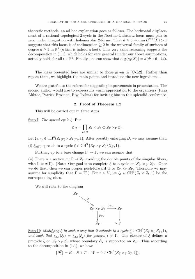
We will refer to the diagram
ZΓ
Δ
�����������
ZΓ ×Γ ZΓPr1 ��
Pr2
��
ZΓ
��ZΓ
�� Γ
Step II: Modifying ξ in such a way that it extends to a cycle ξ ∈ CH3(ZΓ×ΓZΓ, 1),and such that r3,1(ξt) = r3,1(ξt) for general t ∈ Γ. The closure of ξ defines a
precycle ξ on ZΓ ×Γ ZΓ whose boundary ∂ξ is supported on ZB . Thus accordingto the decomposition in (1.1), we have
{∂ξ} = R + S + T +W = 0 ∈ CH3(ZΓ ×Γ ZΓ;Q),
26 XI CHEN AND JAMES D. LEWIS
where
R =∑t∈B
Zt ⊗ ξ(R)t , S =
∑t∈B
ntHt ⊗H ′t
T =∑t∈B
ξ(T )t ⊗ Zt, W =
∑t∈B
mtΔZt
Here Ht and H ′t are general hyperplane sections of Zt, ξ
(R)t , ξ
(T )t are 0-cycles, and
nt, mt ∈ Q. Now put
D1 =∐t∈Γ
σ(t)× Zt � ZΓ
D2 =∐t∈Γ
Zt × σ(t) � ZΓ
H =∐t∈Γ
H ′t ⊗Ht
Δ = Δ(ZΓ)
Let d = degZt =(H2
t
)Zt, and put ξ = R+ S + T +W . Also put N =
(Δ2
Zt
)Zt×Zt
for any t ∈ U . Of course, this number is really independent of t ∈ Γ, by definingit as a limit t �→ t0 over t ∈ U , for any t0 ∈ Γ; and observe that for t ∈ U ,N = deg(c2(Zt)).
We compute:
ξ ∩D1 =∑t∈B
σ(t)× ξ(R)t +
∑t∈B
mt(σ(t), σ(t)) ∼rat 0 on D1
ξ ∩D2 =∑t∈B
ξ(T )t × σ(t) +
∑t∈B
mt(σ(t), σ(t)) ∼rat 0 on D2
These equations yield:
∑t∈B
([deg(ξ
(R)t )
]· t+mt · t
)∼rat 0 on Γ
∑t∈B
([deg(ξ
(T )t )
]· t+mt · t
)∼rat 0 on Γ
Further,
ξ ∩H ∼rat 0 ⇒ d2(∑t∈B
nt · t)+ d
∑t∈B
mt · t ∼rat 0 on Γ
⇒ d(∑t∈B
nt · t)+
∑t∈B
mt · t ∼rat 0 on Γ
ξ ∩Δ ∼rat 0 ⇒ d(∑t∈B
nt · t)+N
∑t∈B
mt · t
+∑t∈B
[deg(ξ
(R)t )
]· t+
∑t∈B
[deg(ξ
(T )t )
]· t ∼rat 0 on Γ
REGULATOR FOR A SELF-PRODUCT OF A GENERAL SURFACE 27
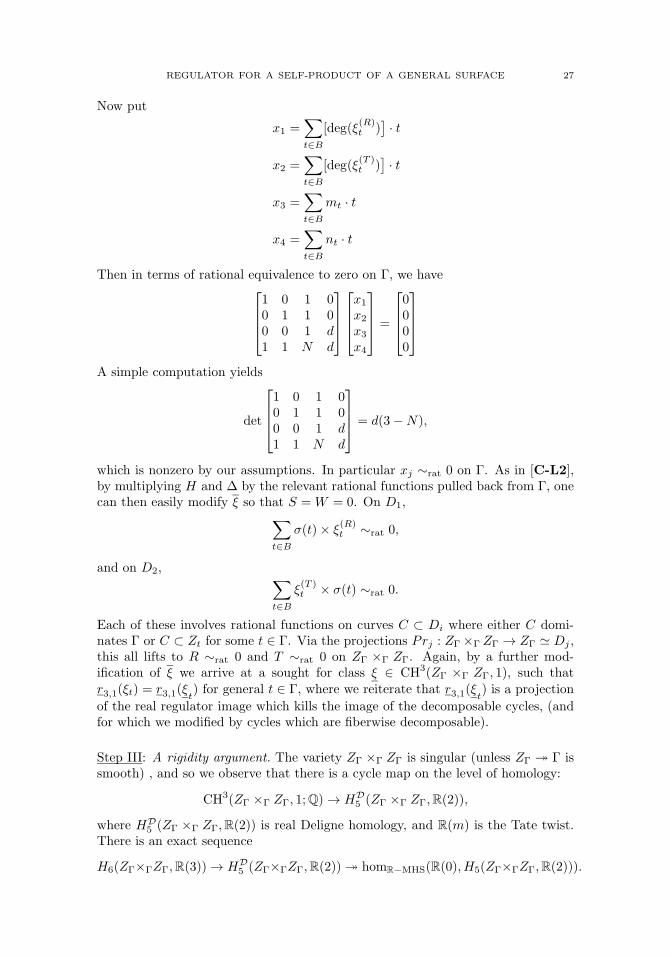
Now put
x1 =∑t∈B
[deg(ξ(R)t )
]· t
x2 =∑t∈B
[deg(ξ(T )t )
]· t
x3 =∑t∈B
mt · t
x4 =∑t∈B
nt · t
Then in terms of rational equivalence to zero on Γ, we have⎡⎢⎢⎣1 0 1 00 1 1 00 0 1 d1 1 N d
⎤⎥⎥⎦⎡⎢⎢⎣x1
x2
x3
x4
⎤⎥⎥⎦ =
⎡⎢⎢⎣0000
⎤⎥⎥⎦
A simple computation yields
det
⎡⎢⎢⎣1 0 1 00 1 1 00 0 1 d1 1 N d
⎤⎥⎥⎦ = d(3−N),
which is nonzero by our assumptions. In particular xj ∼rat 0 on Γ. As in [C-L2],by multiplying H and Δ by the relevant rational functions pulled back from Γ, onecan then easily modify ξ so that S = W = 0. On D1,∑
t∈B
σ(t)× ξ(R)t ∼rat 0,
and on D2, ∑t∈B
ξ(T )t × σ(t) ∼rat 0.
Each of these involves rational functions on curves C ⊂ Di where either C domi-nates Γ or C ⊂ Zt for some t ∈ Γ. Via the projections Prj : ZΓ ×Γ ZΓ → ZΓ � Dj ,this all lifts to R ∼rat 0 and T ∼rat 0 on ZΓ ×Γ ZΓ. Again, by a further mod-ification of ξ we arrive at a sought for class ξ ∈ CH3(ZΓ ×Γ ZΓ, 1), such thatr3,1(ξt) = r3,1(ξt) for general t ∈ Γ, where we reiterate that r3,1(ξt) is a projection
of the real regulator image which kills the image of the decomposable cycles, (andfor which we modified by cycles which are fiberwise decomposable).
Step III: A rigidity argument. The variety ZΓ ×Γ ZΓ is singular (unless ZΓ � Γ issmooth) , and so we observe that there is a cycle map on the level of homology:
CH3(ZΓ ×Γ ZΓ, 1;Q) → HD5 (ZΓ ×Γ ZΓ,R(2)),
where HD5 (ZΓ ×Γ ZΓ,R(2)) is real Deligne homology, and R(m) is the Tate twist.
There is an exact sequence
H6(ZΓ×ΓZΓ,R(3)) → HD5 (ZΓ×ΓZΓ,R(2)) � homR−MHS(R(0), H5(ZΓ×ΓZΓ,R(2))).
28 XI CHEN AND JAMES D. LEWIS
We will show (below) that the cycle ξ ∈ CH3(ZΓ ×Γ ZΓ, 1;Q) has zero image in
homR−MHS
(R(0), H5(ZΓ ×Γ ZΓ,R(2))
). Hence we can assume that ξ ∈ HD
5 (ZΓ ×Γ
ZΓ,R(2)) lifts to a class in H6(ZΓ ×Γ ZΓ,R(3)). Now consider the composite
H6(ZΓ×ΓZΓ,R(3)) → H4(Zt×Zt,R(2))∼→H4(Zt×Zt,R(2)) � H2,2(Zt×Zt,R(2)).
Then as in [C-L1], we can apply Betti rigidity, together with our monodromyassumptions to deduce that r3,1(ξt) (a fortiori r3,1(ξt)) is zero for sufficiently generalt ∈ Γ. We now attend to the details of modifying ξ. In local analytic coordinatesthe singular set of ZΓ ×Γ ZΓ looks like
x21 + x2
2 + x23 = tM = y21 + y22 + y23 ,
for some positive integer M . Since we assume ZΓ to be smooth, we necessarily haveM = 1. Then locally we are in the situation of
x21 + x2
2 + x23 − (y21 + y22 + y23) = 0,
which is an isolated nodal singularity. Then the projectivized tangent cone is a4-dimensional smooth quadric Q0 whose generators contribute to the vector space
homR−MHS
(R(0), Gr0WH5(ZΓ ×Γ ZΓ,R(2))
). Let ˜[ZΓ ×Γ ZΓ]0 be the blow-up of
ZΓ ×Γ ZΓ at this isolated singular point 0. Now recall by assumption that we have
an injection CH2(Q0;Q) ↪→ CH3( ˜[ZΓ ×Γ ZΓ]0;Q). From the localization sequence
· · · → CH3( ˜[ZΓ ×Γ ZΓ]0, 1;Q) → CH3(ZΓ ×Γ ZΓ\{0}, 1;Q)
→ CH2(Q0;Q) ↪→ CH3( ˜[ZΓ ×Γ ZΓ]0;Q) → · · · ,
it is clear that ξ lifts to a class in CH3( ˜[ZΓ ×Γ ZΓ]0, 1;Q). Repeating this procedurefor each nodal singularity, we arrive at ξ lying in the image of
CH3( ˜ZΓ ×Γ ZΓ, 1;Q) → CH3(ZΓ ×Γ ZΓ, 1;Q),
where ˜ZΓ ×Γ ZΓ is a desingularization of ZΓ×ΓZΓ. Now use the fact that the space
homR−MHS
(R(0), H5( ˜ZΓ ×Γ ZΓ,R(2))
)= 0. �
Remark 2.1. Let us put
Zt =
{Zt if Zt smooth
desing(Zt) if Zt singular
where desing(Zt) is the minimal desingularization of Zt. Suppose that
H2,2(Zt × Zt)⋂
H2tr(Zt,Q)⊗H2
tr(Zt,Q) � Q,
and that
CH1(Zt;Q) � Q,
for all t ∈ Γ. (This last condition implies that H1(Zt,Q) = 0 = H3(Zt,Q).) Thenassuming the existence of the conjectured Bloch-Beilinson filtration, one can showas in [C-L2] that the decomposition in (1.1) holds.

REGULATOR FOR A SELF-PRODUCT OF A GENERAL SURFACE 29
3. Proof of Theorem 1.3
Let ZP1 ⊂ P1 × P3 be a Lefschetz pencil of surfaces of degree d in P3 withP1 ⊂ PN . For a very general choice of P1 ⊂ PN , we can make it avoid Σ and thelocus where Pic(Zt) �= Z. Suppose that we have a class ξt ∈ CH3(Zt × Zt, 1;Q)for t ∈ P1 general. Then after a base change Γ → P1, we can extend ξt to ξUover an open set U ⊂ Γ. By the same argument in the previous section, we canfurther extend ξ to all of ZΓ ×Γ ZΓ, where ZΓ = ZP1 ×P1 Γ. As mentioned at verybeginning, ZΓ might be singular. Hence, in order to show the vanishing of r3,1(ξ)by the monodromy argument, we need to lift ξ to a desingularization of ZΓ ×Γ ZΓ.
We first desingularize ZΓ. Let Y be the minimal desingularization of ZΓ. Ob-serve that the singularities of ZΓ consist of the points p ∈ Zt, where p is an ordinarydouble point of the surface Zt and the finite map Γ → P1 is ramified at t ∈ Γ. Lo-cally at p, ZΓ is given by
(3.1) x21 + x2
2 + x23 = tM
where M is ramification index Γ → P1 at t. For simplicity, we may assume that Mis even; otherwise, we just replace Γ by Γ′ with a further base change Γ′ → Γ. Thesingularity p as in (3.1) can be resolved by a sequence of blowups and we end upwith
Yt = Zt ∪Q1 ∪Q2 ∪ ... ∪Qm
locally over p, where Q0 = Zt is the proper transform of Zt and Q1, Q2, ..., Qm area chain of m = M/2 rational ruled surfaces satisfying that
• Qi∼= F2 for 1 ≤ i ≤ m− 1 and Qm
∼= F0 = P1 × P1;• Qi ∩Qj �= ∅ iff |i− j| ≤ 1;• Qi−1 and Qi meet transversely along a curve Ci
∼= P1 for i = 1, 2, ...,m.
Let us consider Y ×Γ Y . This is only a partial resolution of ZΓ ×Γ ZΓ; Y ×Γ Yis singular along Ci × Cj with local equation x1x2 = y1y2 = t. On the other
hand, Y ×Γ Y admits a small resolution ˜Y ×Γ Y and we can lift every class in
CH3(Y ×Γ Y, 1;Q) to CH3( ˜Y ×Γ Y , 1;Q). This small resolution is obtained bysubsequently blowing up Qi × Qj ; locally we are blowing up along x1 = y1 = 0.
Note that ˜Y ×Γ Y is projective as it is obtained by blowing up along algebraicsubvarieties. The exceptional loci of this resolution consist of threefolds Eij whichare P1 bundles over Ci × Cj for 1 ≤ i, j ≤ m. So the obstruction to the liftingcomes from the map
(3.2)⊕i,j
CH1(Eij ;Q) → CH3( ˜Y ×Γ Y ;Q)
by the corresponding localization sequence; a class in CH3(Y ×Γ Y, 1;Q) can be
lifted to CH3( ˜Y ×Γ Y , 1;Q) if the map (3.2) is injective.
Let Qi ×Qj ⊂ ˜Y ×Γ Y be the proper transform Qi ×Qj . The 3-fold Eij is theintersection of two out of the four 4-folds among
{ ˜Qi−α ×Qj−β : α, β = 0 or 1}
and meets the other two transversely along two disjoint sections of Eij → Ci ×Cj ,say Gij and G′
ij ⊂ Eij ; exactly which two depends on the order in which we blow
30 XI CHEN AND JAMES D. LEWIS
up Qi ×Qj . Obviously,
(3.3) CH1(Eij) ∼= CH1(Ci × Cj)⊕ ZGij .
On Y , we obviously have the injection
(3.4)⊕i
CHk(Ci) ↪→ CHk+2(Y )
for k = 0, 1. This gives us the injection
(3.5)⊕i,j
CH1(Ci × Cj) ↪→ CH3( ˜Y ×Γ Y ).
On the other hand, it is easy to show the injection
(3.6)⊕i,j
(ZGij ⊕ ZG′ij) ↪→ CH3( ˜Y ×Γ Y )
and the injectivity of (3.2) follows.So it remains to lift classes in CH3(Z ×Γ Z, 1;Q) to CH3(Y ×Γ Y, 1;Q). The
obstruction is the map
(3.7)⊕i,j
CH2(Qi ×Qj ;Q) → CH3(Y ×Γ Y ;Q)
and it suffices to show that (3.7) is injective.Obviously,
(3.8) CH2(Qi ×Qj) =
2⊕k=0
CHk(Qi)⊗CH2−k(Qj)
and the injections
(3.9) CHk(Qi) ↪→ CHk+1(Y )
are trivial for k = 0, 2. The hard part is to prove (3.9) for k = 1, i.e.,
(3.10)⊕i
CH1(Qi) ↪→ CH2(Y ).
This has been done in the appendix of [C-L2], where it was proved that (3.10) isan injection if ZP1 is chosen to be a very general pencil.
References
[B] S. Bloch, Algebraic cycles and higher K-theory, Advances in Math. 61 (1986), 267-304.[C-L1] X. Chen and J. D. Lewis, Noether-Lefschetz for K1 of a certain class of surfaces, Bol. Soc.
Mat. Mexicana 10(3) (2004), 29-41.[C-L2] X. Chen and J. D. Lewis, The real regulator for a product of K3 surfaces, in Mirror
Symmetry V, Proceedings of the BIRS conference in Banff, Alberta (Edited by S.-T. Yau,N. Yui and J. D. Lewis), AMS/IP Studies in Advanced Mathematics, Volume 38. (2006),271-283.
[C-L3] X. Chen and J. D. Lewis, Real Regulators on Self-products of K3 Surfaces. To appear inthe J. of Algebraic Geometry.
[C-L4] X. Chen and J. D. Lewis, The Hodge-D-conjecture for K3 and Abelian surfaces, J. Alg.Geom. 14 (2005), 213-240.
[G] M. Green, A new proof of the explicit Noether-Lefschetz theorem, J. Differential Geometry27 (1988), 155-159.
[L] J. D. Lewis, A filtration on the Chow groups of a complex projective variety, CompositioMath. 128, (2001), 299-322.

REGULATOR FOR A SELF-PRODUCT OF A GENERAL SURFACE 31
632 Central Academic Building, University of Alberta, Edmonton, Alberta T6G
2G1, CANADA
E-mail address: [email protected]
632 Central Academic Building, University of Alberta, Edmonton, Alberta T6G
2G1, CANADA
E-mail address: [email protected]


Clay Mathematics ProceedingsVolume 9, 2010
Lipschitz Cocycles and Poincare Duality
Eric M. Friedlander∗ and Christian Haesemeyer∗∗
Abstract. Geometric measure theory enables one to view cohomology asequivalence classes of graphs of multi-valued Lipschitz maps to spheres. Thisgeometric point of view gives a new formulation of cohomology, relative co-homology, and cohomology with supports as homotopy groups of spaces ofLipschitz cocycles. Using the graphing construction of the first author and
H. Blaine Lawson, this leads to a formulation and proof of weak equivalenceswhose associated map on homotopy groups is a form of Alexander duality forthe complement of a compact subpolyhedron in a compact, oriented smoothmanifold.
0. Introduction
Let A be a compact oriented n-dimensional pseudo-manifold which is smooth-able outside a subcomplex of codimension 2 and let α ∈ Hj(A,Z) be an integralcohomology class of A. In [6], the first author and H. Blaine Lawson established thatα∩ [A] ∈ Hn−j(A) can be represented by the geometric measure-theoretic slice ofthe graph of a multi-valued Lipschitz map from A to Sj . The purpose of this paperis to extend the constructions of [6] to a compactifiable pseudo-manifold A − A∞and then use this extension to prove a form of Alexander duality whenever A−A∞ issmooth. Indeed, we prove a stronger result which is the geometric measure-theoreticanalogue of the Friedlander-Lawson [5] and Friedlander-Voevodsky [7] duality the-orems for smooth complex algebraic varieties. Namely, as seen in Corollary 5.5, thegraphing construction for Lipschitz maps determines a weak equivalence relatingthe topological abelian groups of Lipschitz cocycles on A−A∞ and an appropriategroup of rectifiable currents on A with boundary in a closed tubular neighborhoodof A∞.
Our arguments involve a mixture of elementary simplicial topology and geo-metric measure theory. The fundamental construction Γtop involves the graphingof a multi-valued Lipschitz map to a sphere with domain a compact oriented n-dimensional pseudo-manifold A equipped with a triangulation. Such a space is aLipschitz neighborhood retract, admitting a good formulation of currents. More-over, the triangulation enables us to work cell-by-cell, enabling local arguments andconsideration of subcomplexes and their complements.
∗ partially supported by NSF # 03000525.∗∗ partially supported by NSF # 0924631.
c© 2010 Eric M. Friedlander and Christian Haesemeyer
33
34 ERIC M. FRIEDLANDER AND CHRISTIAN HAESEMEYER
To summarize in more detail, Section 1 introduces the open and closed sub-sets of polyhedra which we shall employ, and discusses various spaces of Lipschitzmaps with target a symmetric product of a sphere. In Section 2, we define theLipschitz cocyle space Zm(A) of codimension m cocycles on a finite polyhedron A,the relative cocyle space Zm(A,C) for a closed subset C ⊂ A, the cocycle spaceZm(A − A∞) of codimension m Lipschitz cocycles on the complement of a closedsubpolyhedron A∞ ⊂ A, and the space Zm
A∞(A) of codimension m Lipschitz cocy-
cles on A with support in A∞. Essentially, a Lipschitz cocycle on A is an element ofthe group completion of spaces of Lipschitz maps from A into symmetric powers ofa sphere. As seen in Section 3, the homotopy groups of these cocycle spaces satisfythe expected properties of singular cohomology.
The first author and H. Blaine Lawson constructed in [6] a continuous graphmapping Γtop : Zm(A) → Zn(A×Sm) for A a compact, oriented pseudo-manifold ofdimension n. This graphing construction was shown to yield cap product with thefundamental class of A, so that Poincare Duality could be interpreted in these terms.In Theorem 4.5, we extend this continuous graphing construction to Zm(A−A∞).With the formalism established for A − A∞, we not only can formulate variousduality theorems for non-compact spaces but also give proofs which use only thetechniques developed in this paper. For example, Corollary 5.5 is a formulation interms of spaces of cocycles/cycles of Poincare-Alexander duality.
In the final section, we show how the Thom class and the Thom isomorphismadmit a natural formulation in terms of Lipschitz cocycles.
We thank Blaine Lawson for sharing with us his geometric insight into Poincareduality.
1. Polyhedra, rectifiable currents, and Lipschitz Maps
We consider a compact polyhedron A, a cell complex which is the geometricrealization of a finite simplicial complex. We shall typically consider a (piece-wiselinear) triangulation Δ on A associated to some choice of structure of a finite sim-plicial complex, and then consider refinements of such a triangulation. By abuse ofnotation, we shall refer to a compact polyhedron together with a given (finite, piece-wise linear) triangulation as a simplicial complex as well. We denote by Δ(k) the(finite) set of open k-simplices of Δ, each homeomorphic to an open k-disk. Observethat the d-fold symmetric product SP d(A) of A is again a compact polyhedron.
If A is a compact polyhedron, then a simplicial structure on A determines anembedding of A in a Euclidean space RN , where N denotes the number of verticesof the simplicial structure. A tubular neighborhood of A ⊂ RN provides A with thestructure of a Lipschitz neighborhood retract of RN . Such an embedding providesA with a piecewise smooth Riemannian metric (compatible with the triangulationon A given by the simplicial structure). The class of Lipschitz functions associatedto such a metric on A is in fact independent of the choice of such a metric.
Definition 1.1. Let A be a compact polyhedron, a Lipschitz neighborhoodretract with Lipschitz retraction U → A of some tubular neighborhood U of A ina Euclidean space. A polyhedral k-chain on a Euclidean space is a formal integralsum of “k-prisms” defined as the convex hulls of (k + 1)-tuples of distinct points,and a Lipschitz polyhedral k-chain on A is the image of such a polyhedral chainunder a Lipschitz map from a Euclidean space to A. A rectifiable k-current on A is

LIPSCHITZ COCYCLES AND POINCARE DUALITY 35
an element in the closure (with respect to the mass norm) of the space of Lipschitzpolyhedral k-chains on A.
We denote by Ik(A) the space of rectifiable k-currents on A with rectifiableboundary (i.e., integral k-currents) equipped with the flat norm topology. Wedenote by Zk(A) ⊂ Ik(A) the subspace of rectifiable k-currents with 0-boundary(i.e. integral k-cycles).
We recall the following theorem of F. Almgren [1] (and restated in [6, 1.2]).
Theorem 1.2. Let C ⊂ A be a closed subspace, with both A,C compact, lo-cal Lipschitz neighborhood retracts in Euclidean spaces. Then there is a naturalisomorphism
A : πj{Zr(A,C)/Ir(C)} ∼−→ Hr+j(A,C).
Here, Ir(C) denotes the integral r-currents on C with the flat norm topology andZr(A,C) denotes the integral r-currents on A whose boundary has support in C,also provided with the flat norm topology.
Moreover, Zr(A)/Zr(C) is a closed subspace of Zr(A,C)/Ir(C) with discretequotient, thereby determining the short exact sequence
0 → Zr(A)/Zr(C) → Zr(A,C)/Ir(C) → ker{Hr−1(C) → Hr−1(A)} → 0.
We shall work with non-compact spaces of the form A − A∞, where A is acompact polyhedron and A∞ ⊂ A is a (closed) subcomplex with respect to somefinite triangulation of A. We shall refer to such a space A−A∞ as a compactifiablepolyhedron.
Definition 1.3. Let A be a finite polyhedron. Equip A with a (finite, piece-wise linear) triangulation Δ and let A∞ ⊂ A be a closed subpolyhedron that is asubcomplex for the triangulation Δ. Embed A in Euclidean space Rs, where s is thenumber of vertices of A, so that each vertex is a distance 1 along the correspondingaxis of Rs.
We define
DΔ(A∞) ≡ {a ∈ A : dA(a,A∞) ≤ 1
4}
OΔ(A∞) ≡ {a ∈ A : dA(a,A∞) <1
4}
SΔ(A∞) ≡ {a ∈ A : dA(a,A∞) =1
4}
Note that DΔ(A∞), SΔ(A∞) and A−OΔ(A∞) are all closed subcomplexes ofA for some suitable subdivision of the triangulation Δ. It is useful to observe thatif Δ′ refines Δ then OΔ′(A∞) ⊂ OΔ(A∞).
The following proposition constructs a flow from A − A∞ to the closed sub-polyhedron A−OΔ(A∞).
Proposition 1.4. Let U = A−A∞ be a compactifiable polyhedron.
(1) There is a homotopy H : U × I → U relating the identity of U to aretraction U → A−OΔ(A∞) and restricting to H| : (A−OΔ(A∞))× I →A−OΔ(A∞).
(2) There is a deformation retraction F : DΔ(A∞) × I → DΔ(A∞) which isa deformation retraction to the subpolyhedron A∞.

36 ERIC M. FRIEDLANDER AND CHRISTIAN HAESEMEYER
Proof. Observe that the closure σ of an open simplex of A meets DΔ(A∞) ifand only if σ meets A∞. Let Y ⊂ A denote the union of those closed simplices of Ameeting A∞, and triangulate Y using the first barycentric subdivision of the giventriangulation of A. We define the “link” L ⊂ A of A∞ ⊂ A to be the sub-simplicialcomplex of Y with vertices the barycenters of simplices of A whose closures do notintersect A∞. Let L ⊂ Y consist of those points y ∈ Y ; d(y, L) ≤ 1
4 . Then weemploy a continuous map
F : Y × I → Y
satisfying
• F (y, 0) = y, y ∈ Y• F (x, t) = x, x ∈ A∞ and t ∈ I
• F (y, t) = y, y ∈ L and t ∈ I• F (−, t) is a homeomorphism for t �= 1• F (DΔ(A∞)× {1})) ⊂ A∞• F (DΔ(A∞)× I) ⊂ DΔ(A∞).
Any such map F restricted to DΔ(A∞) is a deformation retraction to A∞.Moreover, , we obtain a deformation retraction F ′ : (Y − A∞) × I → Y − A∞ ofY − A∞ to Y − DΔ(A∞) by setting F ′
t equal to the inverse of the restriction toY −A∞ of F1−t. We define H : U × I → I to be this retraction on (Y − A∞)× Iand the identity flow on (A− Y )× I. �
We shall use the following elementary lemma from homotopy theory.
Lemma 1.5. Let Y ⊂ X be an inclusion of a subspace of a topological space X.Suppose there is a homotopy H : X × I → X such that
• H(−, 0) = idX• H(X × {1}) ⊂ Y• H(Y × {t}) ⊂ Y for all t.
Then the inclusion Y → X is a homotopy equivalence with homotopy inverseH(−, 1).
Applying Lemma 1.5 to the homotopy of Proposition 1.4 (1), we immediatelyobtain the following corollary.
Corollary 1.6. Let U = A − A∞ be a compactifiable polyhedron and let Δbe some finite piece-wise linear triangulation of A such that A∞ is a subcomplex.Then the embedding
A′ = (A−OΔ(A∞)) ⊂ U
is a weak equivalence and A′ is a compact polyhedron.
We recall that a continuous map f : A → B of metric spaces is said to beLipschitz with Lipschitz constant K if for all pairs of points a, a′ in A the followinginequality is satisfied:
dB(f(a), f(a′)) ≤ K · dA(a, a′).
Definition 1.7. If A, B are metric spaces, then we define
MapLip(A,B)
to be the set of Lipschitz maps from A to B with topology of convergence withbounded Lipschitz constant. In other words, the sequence {fn} converges to f :

LIPSCHITZ COCYCLES AND POINCARE DUALITY 37
A → B in this topology if it is uniformly convergent and there is a K > 0 thatserves as Lipschitz constant for all the fn.
Remark 1.8. If A and B are compact polyhedra equipped with a piecewisesmooth metric via embeddings as Lipschitz neighborhood retracts, then the subset
MapLip(A,B) ↪→ Mapcont(A,B)
together with its topology is independent of the choice of embedding. On thestrength of this observation we will refer to its elements as Lipschitz maps from Ato B without reference to the specific piecewise smooth metric chosen.
Observe that if B is a compact polyhedron, then so is its d-fold symmetricpower SP d(B) for any d > 0.
In [6, 1.5], the embedding MapLip(A,SP d(Sm)) ↪→ Mapcont(A,SP d(Sm)) isshown to be a weak homotopy equivalence. We extend this result by allowing A tobe a compactifiable polyhedron.
Proposition 1.9. Let A, B be compact polyhedra, and d > 0. Retain thehypotheses and notation of Definition 1.3. Then each of the maps of the followingchain is a weak homotopy equivalence
Mapcont(A−A∞, SP d(B)) → Mapcont(A−OΔ(A∞), SP d(B)) ←MapLip(A−OΔ(A∞), SP d(B)).
Proof. The homotopy H : U × I → U of Proposition 1.4 implies that the firstmap is a homotopy equivalence by Lemma 1.5; [6, 1.5] verifies that the second mapis a weak equivalence. �
Lemma 1.10. If Δ′ is a refinement of the triangulation Δ of A, then for anyd > 0 the natural restriction map
MapLip(A−OΔ′(A∞), SP d(B)) → MapLip(A−OΔ(A∞), SP d(B))
is a Serre fibration and a weak equivalence.
Proof. Let Λj [n] ⊂ Δ[n] denote the inclusion of the union of all faces of the n-simplex Δ[n] except the j-th face into Δ[n]. For each n ≥ 0 and each j, 0 ≤ j ≤ n,we use the structure of A−OΔ(A∞) ⊂ A−OΔ′(A∞) (as a simplicial embedding offinite complexes) to exhibit a strong deformation retraction of (A−OΔ′(A∞))×Δ[n]to
((A−OΔ′(A∞))× Λj [n]) ∪((A−OΔ(A∞))×Λj [n]) ((A− OΔ(A∞))×Δ[n])
which is a Lipschitz map with Lipschitz constant 1. This implies the Serre liftingproperty forMapLip(A−OΔ′(A∞), SP d(Sm)) → MapLip(A−OΔ(A∞), SP d(Sm)).The fact that this map is a weak equivalence follows from Proposition 1.9 and thefact that both A−OΔ(A∞), A−OΔ′(A∞) are homotopy equivalent to A−A∞. �
Definition 1.11. Let T (A) denote the category of finite, piece-wise lineartriangulations of the polyhedron A, with one triangulation Δ′ mapping to anotherΔ provided that Δ′ is a refinement of Δ. For any closed subpolyehdron A∞ ⊂ Awhich is a subcomplex with respect to a triangulation Δ, any finite polyhedron Band any d > 0, we define
(1) MapbLip(A−A∞, SP d(B)) ≡ lim←−Δ′∈T (A)/Δ
MapLip(A−OΔ′(A∞), SP d(B)).

38 ERIC M. FRIEDLANDER AND CHRISTIAN HAESEMEYER
Remark 1.12. Let A, A′, B be finite polyhedra and let A∞ ⊂ A, A′∞ ⊂ A′
be subpolyhedra. Then a Lipschitz map f : A → A′ with the property thatf−1(A′
∞) ⊂ A∞ induces a continuous map
(2) f∗ : MapbLip(A′ −A′
∞, SP d(B)) −→ MapbLip(A−A∞, SP d(B)).
In particular, there is a natural restriction map
MapbLip(A−A′∞, SP d(B)) → MapbLip(A−A∞, SP d(B))
whenever A′∞ ⊂ A∞ is an inclusion of closed subcomplexes for some finite triangu-
lation. This implies that the assignment
U �→ MapbLip(U, SPd(B))
is a contravariant functor on the category of open subsets of A whose complementis a closed subcomplex for some sufficiently fine finite triangulation of A.
Corollary 1.13. The natural projection and inclusion maps
MapLip(A−OΔ(A∞), SP d(B)) � MapbLip(A−A∞, SP d(B))
and
MapbLip(A− A∞, SP d(B)) ↪→ Mapcont(A−A∞, SP d(B))
are weak equivalences for any finite, piece-wise linear triangulation Δ of A suchthat A∞ inherits the structure of a subcomplex.
Proof. The fact that the projection is a weak equivalence follows from Lemma1.10 and the standard fact that the inverse limit of a tower of maps each of whichis a Serre fibration and a weak equivalence projects via a Serre fibration and aweak equivalence to each term in the tower. The fact that the inclusion is a weakequivalence follows from Proposition 1.9. �
2. Lipschitz cocycle spaces
Recall that the group completion (∐
d SPd(Sm))+ is a model for the generalized
Eilenberg-MacLane space K(Z,m)×K(Z, 0), so that
πi(Mapcont(A, (∐d
SP d(Sm))+) =
⎧⎨⎩
Hm(A)⊕H0(A) if i = 0
Hm−i(A) if i > 0.
where Hi(A) = Hi(A,Z) denotes singular cohomology with Z coefficients. Since Ais compact,
(∐d
Mapcont(A,SP d(Sm))+ ∼= Mapcont(A, (∐d
SP d(Sm))+).
Thus,
πi ker{(∐d
Mapcont(A,SP d(Sm))+ → H0(A)} ∼= Hi(A), i ≥ 0.
This motivates the following definition of Lipschitz cocycle spaces. We set
(3) MapLip(A,SP∞(Sm)+) = ker{(∐d≥0
MapLip(A,SP d(Sm)))+ → H0(A)}.
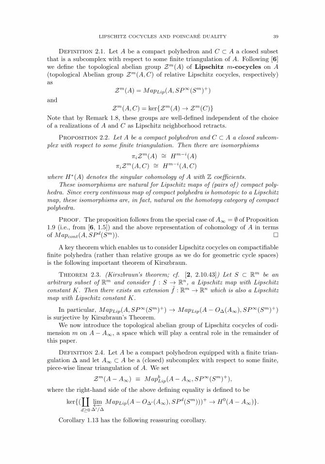
LIPSCHITZ COCYCLES AND POINCARE DUALITY 39
Definition 2.1. Let A be a compact polyhedron and C ⊂ A a closed subsetthat is a subcomplex with respect to some finite triangulation of A. Following [6]we define the topological abelian group Zm(A) of Lipschitz m-cocycles on A(topological Abelian group Zm(A,C) of relative Lipschitz cocycles, respectively)as
Zm(A) = MapLip(A,SP∞(Sm)+)
and
Zm(A,C) = ker{Zm(A) → Zm(C)}Note that by Remark 1.8, these groups are well-defined independent of the choiceof a realizations of A and C as Lipschitz neighborhood retracts.
Proposition 2.2. Let A be a compact polyhedron and C ⊂ A a closed subcom-plex with respect to some finite triangulation. Then there are isomorphisms
πiZm(A) ∼= Hm−i(A)
πiZm(A,C) ∼= Hm−i(A,C)
where H∗(A) denotes the singular cohomology of A with Z coefficients.These isomorphisms are natural for Lipschitz maps of (pairs of) compact poly-
hedra. Since every continuous map of compact polyhedra is homotopic to a Lipschitzmap, these isomorphisms are, in fact, natural on the homotopy category of compactpolyhedra.
Proof. The proposition follows from the special case of A∞ = ∅ of Proposition1.9 (i.e., from [6, 1.5]) and the above representation of cohomology of A in termsof Mapcont(A,SP d(Sm)). �
A key theorem which enables us to consider Lipschitz cocycles on compactifiablefinite polyhedra (rather than relative groups as we do for geometric cycle spaces)is the following important theorem of Kirszbraun.
Theorem 2.3. (Kirszbraun’s theorem; cf. [2, 2.10.43]) Let S ⊂ Rm be anarbitrary subset of Rm and consider f : S → Rn, a Lipschitz map with Lipschitzconstant K. Then there exists an extension f : Rm → Rn which is also a Lipschitzmap with Lipschitz constant K.
In particular, MapLip(A,SP∞(Sm)+) → MapLip(A − OΔ(A∞), SP∞(Sm)+)is surjective by Kirszbraun’s Theorem.
We now introduce the topological abelian group of Lipschitz cocycles of codi-mension m on A − A∞, a space which will play a central role in the remainder ofthis paper.
Definition 2.4. Let A be a compact polyhedron equipped with a finite trian-gulation Δ and let A∞ ⊂ A be a (closed) subcomplex with respect to some finite,piece-wise linear triangulation of A. We set
Zm(A−A∞) ≡ MapbLip(A−A∞, SP∞(Sm)+),
where the right-hand side of the above defining equality is defined to be
ker{(∐d≥0
lim←−Δ′/Δ
MapLip(A−OΔ′(A∞), SP d(Sm)))+ → H0(A−A∞)}.
Corollary 1.13 has the following reassuring corollary.
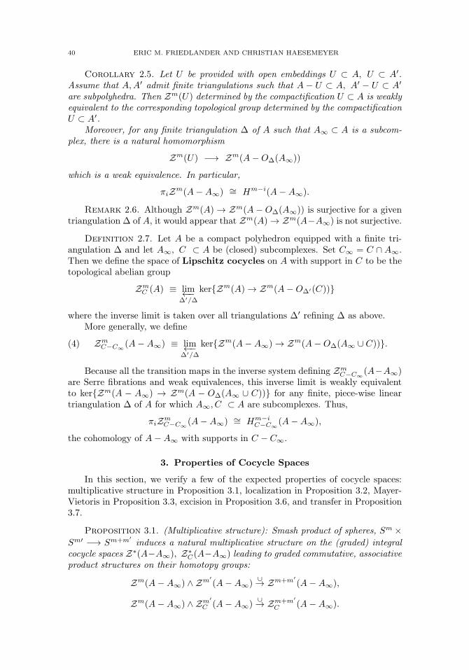
40 ERIC M. FRIEDLANDER AND CHRISTIAN HAESEMEYER
Corollary 2.5. Let U be provided with open embeddings U ⊂ A, U ⊂ A′.Assume that A,A′ admit finite triangulations such that A − U ⊂ A, A′ − U ⊂ A′
are subpolyhedra. Then Zm(U) determined by the compactification U ⊂ A is weaklyequivalent to the corresponding topological group determined by the compactificationU ⊂ A′.
Moreover, for any finite triangulation Δ of A such that A∞ ⊂ A is a subcom-plex, there is a natural homomorphism
Zm(U) −→ Zm(A−OΔ(A∞))
which is a weak equivalence. In particular,
πiZm(A−A∞) ∼= Hm−i(A−A∞).
Remark 2.6. Although Zm(A) → Zm(A−OΔ(A∞)) is surjective for a giventriangulation Δ of A, it would appear that Zm(A) → Zm(A−A∞) is not surjective.
Definition 2.7. Let A be a compact polyhedron equipped with a finite tri-angulation Δ and let A∞, C ⊂ A be (closed) subcomplexes. Set C∞ = C ∩ A∞.Then we define the space of Lipschitz cocycles on A with support in C to be thetopological abelian group
ZmC (A) ≡ lim←−
Δ′/Δ
ker{Zm(A) → Zm(A−OΔ′(C))}
where the inverse limit is taken over all triangulations Δ′ refining Δ as above.More generally, we define
(4) ZmC−C∞(A−A∞) ≡ lim←−
Δ′/Δ
ker{Zm(A−A∞) → Zm(A−OΔ(A∞ ∪ C))}.
Because all the transition maps in the inverse system defining ZmC−C∞
(A−A∞)are Serre fibrations and weak equivalences, this inverse limit is weakly equivalentto ker{Zm(A − A∞) → Zm(A − OΔ(A∞ ∪ C))} for any finite, piece-wise lineartriangulation Δ of A for which A∞, C ⊂ A are subcomplexes. Thus,
πiZmC−C∞(A−A∞) ∼= Hm−i
C−C∞(A− A∞),
the cohomology of A−A∞ with supports in C − C∞.
3. Properties of Cocycle Spaces
In this section, we verify a few of the expected properties of cocycle spaces:multiplicative structure in Proposition 3.1, localization in Proposition 3.2, Mayer-Vietoris in Proposition 3.3, excision in Proposition 3.6, and transfer in Proposition3.7.
Proposition 3.1. (Multiplicative structure): Smash product of spheres, Sm ×Sm′ −→ Sm+m′
induces a natural multiplicative structure on the (graded) integralcocycle spaces Z∗(A−A∞), Z∗
C(A−A∞) leading to graded commutative, associativeproduct structures on their homotopy groups:
Zm(A−A∞) ∧ Zm′(A−A∞)
∪→ Zm+m′(A−A∞),
Zm(A−A∞) ∧ Zm′
C (A−A∞)∪→ Zm+m′
C (A−A∞).

LIPSCHITZ COCYCLES AND POINCARE DUALITY 41
Proof. First, observe that the smash product Sm × Sm′ −→ Sm+m′induces
Lipschitz maps
(5) SP d(Sm)× SP e(Sm′) −→ SP de(Sm+m′
).
Thus, given Lipschitz maps f : A → SP d(Sm), g : A → SP e(Sm′), we obtain the
Lipschitz map f ∧ g : A → SP de(Sm+m′). This determines a pairing of monoids∐
d≥0
MapLip(A,SP d(Sm))×∐e≥0
MapLip(A,SP e(Sm′)) −→
−→∐f≥0
MapLip(A,SP f(Sm+m′)).
The pairings (5) induce the usual product structure K(Z,m) × K(Z,m′) →K(Z,m+m′) which in turn induces the cup product in cohomology. Thus, Propo-sition 2.2 implies that the pairings on homotopy groups of Lipschitz cocycles spacesare graded commutative and associative. �
Proposition 3.2. (Localization) Let A be a compact polyhedron equipped witha finite triangulation Δ and let A∞ ⊂ A be a (closed) subcomplex. Then the naturaltriple of topological abelian groups
(6) ZmA∞(A) → Zm(A) → Zm(A−A∞)
is a fibration sequence.
Proof. For each Δ for which A∞ is a subcomplex of A, the short exact se-quence
ker(Zm(A) → Zm(A− OΔ(A))) → Zm(A) → Zm(A−OΔ(A))
is a fibration sequence by [8]. As argued in the proof of Corollary 1.13, this fibrationsequence is weakly homotopy equivalent to (6). �
Proposition 3.3. (Mayer-Vietoris) Let A be a compact polyhedron equippedwith a finite triangulation Δ and let A∞ ⊂ A be a closed subcomplex. Let D ⊂ A bea compact subpolyhedron containing OΔ(A∞). Then there is a natural short exactsequence of topological abelian groups
Zm(A) → Zm(A−OΔ(A∞))×Zm(D) → Zm(D −OΔ(A∞))
which determines the following homotopy Cartesian square
(7)
Zm(A)
��
�� Zm(D)
��Zm(A−A∞) �� Zm(D −A∞)
.
Proof. Observe that for each Δ for which A∞, D are subcomplexes of A, theshort exact sequence
Zm(A) → Zm(A−OΔ(A∞))×Zm(D) → Zm(D −OΔ(A∞))
is a fibration sequence by [8]. Arguing once again as in the proof of Corollary 1.13in order to pass to the limit over open tubular neighborhoods of A∞, we concludethat
Zm(A) → Zm(A−A∞)×Zm(D) → Zm(D −A∞)
is a fibration sequence. This implies that (7) is homotopy Cartesian. �

42 ERIC M. FRIEDLANDER AND CHRISTIAN HAESEMEYER
Corollary 3.4. Let A be a compact polyhedron and let A∞ ⊂ A and B∞ ⊂ Abe closed subcomplexes with respect to some finite triangulation Δ of A. Assumethere is a finite subdivision Δ′ of Δ such that OΔ′(A∞) ∩ OΔ′(B∞) = ∅. Thenthere is a natural fibration sequence of topological abelian groups
Zm(A) → Zm(A−A∞)×Zm(A−B∞) → Zm(A− (A∞ ∪B∞))
which determines the following homotopy Cartesian square
Zm(A)
��
�� Zm(A−B∞)
��Zm(A−A∞) �� Zm(A− (A∞ ∪B∞))
.
Here the cocycle spaces are taken with respect to the common compactification A,as indicated by the notation.
Proof. This is an immediate consequence of Theorem 3.3 and Corollary 2.5,once we know the various restriction maps are well-defined. This necessary functo-riality property is supplied by the discussion in Remark 1.12. �
Corollary 3.5. Let A be a compact polyhedron and let A∞ ⊂ A and B∞ ⊂ Abe closed subcomplexes with respect to some finite triangulation Δ of A. Then thereis a fibration sequence of topological abelian groups
ZmA∞∩B∞(A) → Zm
A∞(A)× ZmB∞(A) → Zm
A∞∪B∞(A).
Proof. For any refinement Δ′ of Δ, the sequence
(8) ker{Zm(A) → Zm(A−OΔ′(A∞ ∩B∞))}
��ker{Zm(A)×Zm(A) → Zm(A−OΔ′(A∞))×Zm(A−OΔ′(B∞))}
��ker{Zm(A) → Zm(A−OΔ′(A∞ ∪B∞))}
is a fibration sequence by the 3 × 3 lemma and Mayer-Vietoris 3.3 for the closedcover A−OΔ′(A∞ ∩B∞) = (A−OΔ′(A∞)) ∪ (A−OΔ′(B∞)). �
Proposition 3.6. (Excision) Let Δ be a finite triangulation of A and letA∞, D be closed subpolyhedra such that OΔ(A∞) ⊂ D. Then the restriction map
(9) ZmA∞(A) −→ Zm
A∞(D)
is a weak equivalence.
Proof. This follows immediately from Proposition 3.2 applied to the verticalmaps of the homotopy Cartesian square (7). �
Proposition 3.7. (Transfer) Let A, B be finite polyhedra related by a Lipschitzcontinuous map g : A → SP e(B) with associated ramified covering map p : B → A.Assume that A∞ ⊂ A is a nowhere dense closed subpolyhedron with the propertythat p : B −B∞ → A−A∞ is a covering space map, where B∞ = p−1(A∞). Thenp induces a transfer map p! : Zm(B) → Zm(A).

LIPSCHITZ COCYCLES AND POINCARE DUALITY 43
Moreover, the restriction of p! to Zm(B−B∞) has image in Zm(A−A∞) andsatisfies
p∗ ◦ p! = e(−) : Zm(A−A∞) → Zm(B −B∞) → Zm(A−A∞),
where e(−) is the e-th power map of the topological abelian group Zm(A−A∞).
Proof. The map g induces maps g(d) : SP d(A) → SP de(B) in the obviousmanner, and each of these is Lipschitz. These maps determine a map of abelianmonoids ∐
f
MapLip(B,SP f(Sm)) →∐f
MapLip(A,SP d(Sm)
whose group completion is the asserted map p! : Zm(B) → Zm(A).
Choose a triangulation Δ of B with the property that p(Δ) = Δ is a triangu-
lation of A such that with respect to Δ (respectively, Δ) B∞ ⊂ B (resp, A∞ ⊂ A)is a subpolyhedron. Then the restriction of p to B − OΔ(B∞) is a covering spacemap to A−OΔ(A∞). We see by inspection that the composition∐
f
MapLip(B −OΔ(B∞), SP f(Sm)) →∐f
MapLip(A−OΔ(A∞), SP d(Sm)
is multiplication by e. Thus, the second assertion of the proposition follows fromCorollary 1.13. �
4. The Graphing Construction Γtop
The purpose of this section is to establish a continuous graphing map
Γtop : Zm(A−A∞) −→ ˜Zn(A+ ∧ Sm)/ lim−→Δ
Zn(DΔ(A∞)+ ∧ Sm),
where the finite polyhedron A is a compact pseudo-manifold of dimension n. (Fornotational convenience, we employ the abbreviation
(10) Zr(A)/Zr(B) ≡ Zr(A,B)/Ir(B),
the extension of ker{Hr−1(B) → Hr−1(A)} by Zr(A)/Zr(B) given in Theorem1.2.) Our construction extends that of [6] in the case A∞ = ∅, and refines theconstruction there by avoiding the use of the not-everywhere-defined Federer sliceconstruction.
The condition imposed on a compact polyhedron A to be a compact orientedpseudo-manifold of dimension n implies that A has an orientation given by a fun-damental class 0 �= [A] ∈ Hn(A).
We repeat the definition of pseudo-manifold given in [6]. Since our definitionrequires a “resolution of the singularities, all of which are in codimension ≥ 2”, thisis somewhat stronger than that found elsewhere in the literature.
Definition 4.1. Let A be a compact connected polyhedron. A is said to be acompact oriented pseudo-manifold of dimension n if A admits a triangulationΔ satisfying:
• Every simplex of Δ is contained in the closure of some n-simplex τ ∈ Δ(n).• For some smooth closed oriented n-manifold M equipped with a smoothtriangulation, there exists a polyhedral map p : M → A restricting to ahomeomorphism M −M ′ → A−skn−2A, where M ′ ⊂ M is a subcomplexof dimension ≤ n− 2.

44 ERIC M. FRIEDLANDER AND CHRISTIAN HAESEMEYER
If A∞ is a nowhere dense subpolyhedron of the compact oriented pseudo-manifold A of dimension n, then its complement A − A∞ is said to be a com-pactifiable oriented pseudo-manifold of dimension n.
Example 4.2. The underlying analytic space A = Xan of any connected com-plex quasi-projective variety X of complex dimension k is a compactifiable orientedpseudo-manifold of dimension 2k.
If X is a projective variety of dimension n over R whose underlying analyticspace Xan is oriented and connected, then Xan is an compact oriented pseudo-manifold provided that X is smooth in codimension 1.
We proceed to construct the graph of a Lipschitz cocycle f : A − OΔ(A∞) →SP d(Sm). As constructed in [6, 2.4], the geometric graph of f is the rectifiablecurrent
(11) Γ(f) ≡∑σ∈Δ′
Γσ ∈ Rn((A−OΔ(A∞))× Sm),
where the sum is indexed by (open) simplices of A−OΔ(A∞) in a triangulation Δ′
refining Δ with the property that A−OΔ(A∞) is a subcomplex, and Γσ is the push-forward of the simplex σ (viewed as a rectifiable current on A − OΔ(A∞)) to thegraph. Observe that this construction requires A to be provided with an orientationwhich is then inherited in a compatible way by each open simplex σ ∈ Δ′.
There are two awkward aspects of this definition: even for A compact, Γ(f)might not be a cycle; even if Γ(f) is a cycle, the function f �→ Γ(f) might notbe continuous from Lipschitz cocycles to Lipschitz cycles. These difficulties areovercome in [6] by restricting attention to the dense subset of “good” Lipschitzcocycles as we now recall.
Definition 4.3. [6, 3.2] Let B be a finite polyhedron. Choose a compactneighborhood U of SP d(Sm) ⊂ RN and a Lipschitz retraction π : U → SP d(Sm)such that π−1(Σ) is a subcomplex of codimension ≥ 1, where Σ ⊂ SP d(Sm) is thesingular set. A Lipschitz map f : B → SP d(Sm) is said to be good if f is of the
form f = π ◦ f where f when restricted to each open simplex of B is smooth andtransverse to every open simplex of π−1(Σ) ⊂ U .
The following lemma is an immediate consequence of [6, 3.4] and Kirszbraun’sTheorem (Theorem 2.3).
Lemma 4.4. Let A be a compact oriented pseudo-manifold of dimension n, Δa triangulation of A, and A∞ ⊂ A a subpolyhedron, and Δ′ a refinement of Δ suchthat A− OΔ(A∞) is a subcomplex with respect to Δ′. Then the subspace
MapLip(A−OΔ(A∞), SP d(Sm))good ⊂ MapLip(A−OΔ(A∞), SP d(Sm))
of maps f : A − OΔ(A∞) → SP d(Sm) which admit an extension to a good (with
respect to Δ′) Lipschitz map f : A → SP d(Sm) is dense.
Arguing as in [6, 3.6], we obtain the following graphing construction. Weremind the reader that the smash product T+ ∧Sm of a (non-pointed) space T andthe pointed m-sphere (with base point chosen to be ∞ when we view Sm as the1-point compactification of Rm for m > 0 is given by
T+ ∧ Sm ≡ (T × Sm)/(T × {∞}).

LIPSCHITZ COCYCLES AND POINCARE DUALITY 45
Theorem 4.5. Let A be a compact, oriented pseudo-manifold of dimension n,Δ a (piece-wise linear) triangulation of A, and A∞ ⊂ A a subpolyhedron. Thereis a uniquely defined continuous extension
(12) Γtop : Zm(A−OΔ(A∞)) −→ ˜Zn(A+ ∧ Sm)/Zn(DΔ(A∞)+ ∧ Sm),
of the geometric graph construction (11) sending
f ∈ MapLip(A−OΔ(A∞), SP d(Sm))good
to the projection of Γ(f) ∈ Rn((A−OΔ(A∞))× Sm).As Δ varies over finer triangulations of A, these maps determine the continuous
graphing map
(13) Γtop : Zm(A−A∞) −→ ˜Zn(A+ ∧ Sm)/ lim−→Δ
Zn(DΔ(A∞)+ ∧ Sm).
Proof. As constructed in (11), Γ(f) is a rectifiable current on (A−OΔ(A∞))×Sm for any f ∈ MapLip(A−OΔ(A∞), SP d(Sm))good. The continuity of this graph-ing construction
Γ : MapLip(A−OΔ(A∞), SP d(Sm))good −→ Rn((A−OΔ(A∞))× Sm)
is given by [6, 3.5].
Let f : A → SP d(Sm) be a good Lipschitz map extending f . As verified in
[6, 3.6], Γ(f) is an integral n-cycle on A × Sm. Since the restrictions of Γ(f) and
Γ(f) agree on any open inside A − OΔ(A∞), we see that the boundary of Γ(f) issupported on DΔ(A∞)× Sm.
The push-forward of (rectifiable) currents via the proper Lipschitz map (A −OΔ(A∞))× Sm → (A−OΔ(A∞))+ ∧ Sm is that given by Federer in [2, 4.1.7].Thus, for each d ≥ 0, we obtain continuous graphing maps
MapLip(A−OΔ(A∞), SP d(Sm))good → ˜Zn(A+ ∧ Sm)/Zn(DΔ(A∞)+ ∧ Sm)
sending f to the equivalence class of the push-forward of Γ(f).Using Lemma 4.4, we extend this graphing construction to Γtop on MapLip(A−
OΔ(A∞), SP d(Sm)) exactly as in the proof of [6, 3.6], and then use the universalproperty of group completion to obtain the asserted map (12).
Finally, the graphing map Γtop on Zm(A − A∞) of (13) is the (inverse) limitindexed by triangulations Δ of these maps. �
Remark 4.6. Observe that the map in homotopy induced by (13) has the form
Hm−j(A−A∞) −→ HBMn−m+j(A−A∞),
where HBM∗ (−) denotes Borel-Moore (singular) homology.
As we see in the following proposition, Γtop is compatible with localization.Recall the definition of Lipschitz cocycles Zm
C−C∞(A−A∞) given in Definition 4.
Proposition 4.7. (compatibility with localization) Choose a finite triangula-tion Δ of A such that the compact subpolyhedra A∞, C ⊂ A are subcomplexes suchthat DΔ(A∞)∩C = ∅. Then Γtop of (12) restricts to a continuous homomorphismon relative Lipschitz cocycles
(14) Γtop : ZmC (A−OΔ(A∞)) −→ Zn(DΔ(C)+ ∧ Sm)
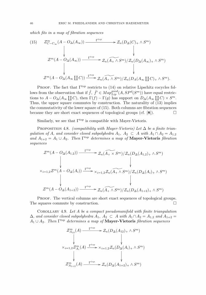
46 ERIC M. FRIEDLANDER AND CHRISTIAN HAESEMEYER
which fits in a map of fibration sequences
(15) ZmC−C∞
(A−OΔ(A∞)) Γtop��
��
Zn(DΔ(C)+ ∧ Sm)
��Zm(A−OΔ(A∞))
Γtop��
��
˜Zn(A+ ∧ Sm)/Zn(DΔ(A∞)+ ∧ Sm)
��Zm(A−OΔ(A∞
∐C))
Γtop�� ˜Zn(A+ ∧ Sm)/Zn(DA(A∞
∐C)+ ∧ Sm).
Proof. The fact that Γtop restricts to (14) on relative Lipschitz cocycles fol-
lows from the observation that if f , f ′ ∈ MapgoodLip (A,SP d(Sm)) have equal restric-
tions to A − OΔ(A∞∐
C), then Γ(f) − Γ(g) has support on DΔ(A∞∐
C) × Sm.Thus, the upper square commutes by construction. The naturality of (13) impliesthe commutativity of the lower square of (15). Both columns are fibration sequencesbecause they are short exact sequences of topological groups (cf. [8]). �
Similarly, we see that Γtop is compatible with Mayer-Vietoris.
Proposition 4.8. (compatibility with Mayer-Vietoris) Let Δ be a finite trian-gulation of A, and consider closed subpolyhedra A1, A2 ⊂ A with A1 ∩A2 = A1,2
and A1+2 = A1 ∪ A2. Then Γtop determines a map of Mayer-Vietoris fibrationsequences
Zm(A−OΔ(A1,2))
��
Γtop�� ˜Zn(A+ × Sm)/Zn(DΔ(A1,2)+ ∧ Sm)
��×i=1,2Zm(A−OΔ(Ai))
Γtop��
��
×i=1,2˜Zn(A+ ∧ Sm)/Zn(DΔ(Ai)+ ∧ Sm)
��Zm(A−OΔ(A1+2))
Γtop�� ˜Zn(A+ ∧ Sm)/Zn(DΔ(A1+2)+ ∧ Sm)
Proof. The vertical columns are short exact sequences of topological groups.The squares commute by construction. �
Corollary 4.9. Let A be a compact pseudomanifold with finite triangulationΔ, and consider closed subpolyhedra A1, A2 ⊂ A with A1∩A2 = A1,2 and A1+2 =A1 ∪A2. Then Γtop determines a map of Mayer-Vietoris fibration sequences
ZmA12
(A)
��
Γtop�� Zn(DΔ(A12)+ ∧ Sm)
��×i=1,2Zm
Ai(A) Γtop
��
��
×i=1,2Zn(DΔ(Ai)+ ∧ Sm)
��Zm
A1+2(A) Γtop
�� Zn(DΔ(A1+2)+ ∧ Sm)
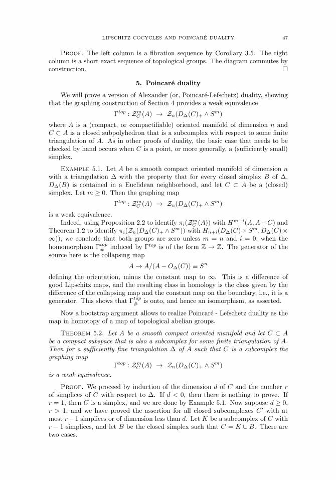
LIPSCHITZ COCYCLES AND POINCARE DUALITY 47
Proof. The left column is a fibration sequence by Corollary 3.5. The rightcolumn is a short exact sequence of topological groups. The diagram commutes byconstruction. �
5. Poincare duality
We will prove a version of Alexander (or, Poincare-Lefschetz) duality, showingthat the graphing construction of Section 4 provides a weak equivalence
Γtop : ZmC (A) → Zn(DΔ(C)+ ∧ Sm)
where A is a (compact, or compactifiable) oriented manifold of dimension n andC ⊂ A is a closed subpolyhedron that is a subcomplex with respect to some finitetriangulation of A. As in other proofs of duality, the basic case that needs to bechecked by hand occurs when C is a point, or more generally, a (sufficiently small)simplex.
Example 5.1. Let A be a smooth compact oriented manifold of dimension nwith a triangulation Δ with the property that for every closed simplex B of Δ,DΔ(B) is contained in a Euclidean neighborhood, and let C ⊂ A be a (closed)simplex. Let m ≥ 0. Then the graphing map
Γtop : ZmC (A) → Zn(DΔ(C)+ ∧ Sm)
is a weak equivalence.Indeed, using Proposition 2.2 to identify πi(Zm
C (A)) with Hm−i(A,A−C) andTheorem 1.2 to identify πi(Zn(DΔ(C)+ ∧Sm)) with Hn+i(DΔ(C)×Sm, DΔ(C)×∞)), we conclude that both groups are zero unless m = n and i = 0, when the
homomorphism Γtop# induced by Γtop is of the form Z → Z. The generator of the
source here is the collapsing map
A → A/(A−OΔ(C)) ≡ Sn
defining the orientation, minus the constant map to ∞. This is a difference ofgood Lipschitz maps, and the resulting class in homology is the class given by thedifference of the collapsing map and the constant map on the boundary, i.e., it is agenerator. This shows that Γtop
# is onto, and hence an isomorphism, as asserted.
Now a bootstrap argument allows to realize Poincare - Lefschetz duality as themap in homotopy of a map of topological abelian groups.
Theorem 5.2. Let A be a smooth compact oriented manifold and let C ⊂ Abe a compact subspace that is also a subcomplex for some finite triangulation of A.Then for a sufficiently fine triangulation Δ of A such that C is a subcomplex thegraphing map
Γtop : ZmC (A) → Zn(DΔ(C)+ ∧ Sm)
is a weak equivalence.
Proof. We proceed by induction of the dimension d of C and the number rof simplices of C with respect to Δ. If d < 0, then there is nothing to prove. Ifr = 1, then C is a simplex, and we are done by Example 5.1. Now suppose d ≥ 0,r > 1, and we have proved the assertion for all closed subcomplexes C ′ with atmost r− 1 simplices or of dimension less than d. Let K be a subcomplex of C withr − 1 simplices, and let B be the closed simplex such that C = K ∪ B. There aretwo cases.

48 ERIC M. FRIEDLANDER AND CHRISTIAN HAESEMEYER
First Case: B is disjoint from K. Then the inductive step follows from the obviousfact that Zm
C (A) ≡ ZmK (A)×Zm
B (A).Second Case: B is not disjoint from K. Then B ∩K = ∂B. Since the dimensionof ∂B is less than d, the inductive hypothesis implies that our assertion holds forthe subcomplexes B, K and ∂B. Now the Mayer-Vietoris sequence of Corollary3.5 and the compatibility of graphing and Mayer-Vietoris given in Corollary 4.9complete the inductive step. �
Remark 5.3. While it may look as if neither orientability nor smoothness isever used in the proof of Theorem 5.2, note that the assumptions are needed forthe graphing construction to work, as discussed in Section 4.
As corollaries, we obtain Poincare Duality and Alexander duality.
Corollary 5.4. Let A be a smooth compact oriented manifold of dimensionn. Then the graphing map
Γtop : Zm(A) → Zn(A+ ∧ Sm)
is a weak equivalence.
Proof. Choose a sufficiently fine triangulation, and let C = A in Theorem5.2. �
Corollary 5.5. Let A be a smooth oriented compact manifold of dimensionn, and let C ⊂ A be a compact subspace that is a subcomplex with respect to somefinite triangulation. Then the graphing map
Γtop : Zm(A− C) −→ ˜Zn(A+ ∧ Sm)/ lim−→Δ
Zn(DΔ(C)+ ∧ Sm)
is a weak equivalence.
Proof. This follows easily from the preceding results and the compatibility ofgraphing with localization proved in Proposition 4.7 (taking A∞ = ∅ in (15) ). �
Definition 5.6. Assume A is a compact, oriented n-manifold and i : A∞ ⊂ Ais a closed, compact, oriented submanifold of codimension e. For any m ≥ e, werefer to the homotopy class of maps
(16) i! = (Γtop)−1 ◦ (i∗ ∧ Σe) ◦ Γtop : Zm−e(A∞) → Zm(A)
as the Gysin map.
Remark 5.7. The map on homotopy groups induced by the Gysin map,
i! : Hm−j−e(A∞) = πj(Zm−e(A∞)) → πj(Zm(A)) = Hm−j(A)
(isomorphic to Hn+j−m(A∞) → Hn+j−m(A)), is the Poincare dual of i∗ : H•(A) →H•(A∞).
6. Thom Classes and Thom Isomorphism
In this last section we formulate the Thom isomorphism in our context.
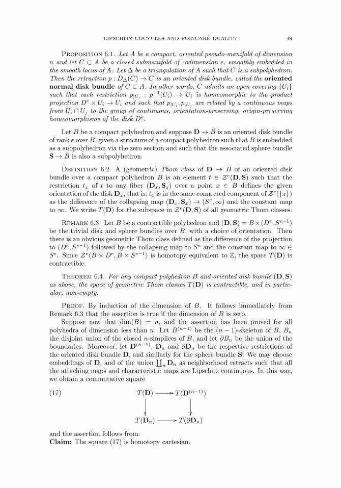
LIPSCHITZ COCYCLES AND POINCARE DUALITY 49
Proposition 6.1. Let A be a compact, oriented pseudo-manifold of dimensionn and let C ⊂ A be a closed submanifold of codimension e, smoothly embedded inthe smooth locus of A. Let Δ be a triangulation of A such that C is a subpolyhedron.Then the retraction p : DΔ(C) → C is an oriented disk bundle, called the orientednormal disk bundle of C ⊂ A. In other words, C admits an open covering {Ui}such that each restriction p|Ui
: p−1(Ui) → Ui is homeomorphic to the productprojection De × Ui → Ui and such that p|Ui
, p|Ujare related by a continuous maps
from Ui ∩ Uj to the group of continuous, orientation-preserving, origin-preservinghomeomorphisms of the disk De.
Let B be a compact polyhedron and suppose D → B is an oriented disk bundleof rank e over B, given a structure of a compact polyhedron such thatB is embeddedas a subpolyhedron via the zero section and such that the associated sphere bundleS → B is also a subpolyhedron.
Definition 6.2. A (geometric) Thom class of D → B of an oriented diskbundle over a compact polyhedron B is an element t ∈ Ze(D,S) such that therestriction tx of t to any fiber (Dx,Sx) over a point x ∈ B defines the givenorientation of the diskDx, that is, tx is in the same connected component of Ze({x})as the difference of the collapsing map (Dx,Sx) → (Se,∞) and the constant mapto ∞. We write T (D) for the subspace in Ze(D,S) of all geometric Thom classes.
Remark 6.3. Let B be a contractible polyhedron and (D,S) = B×(De, Se−1)be the trivial disk and sphere bundles over B, with a choice of orientation. Thenthere is an obvious geometric Thom class defined as the difference of the projectionto (De, Se−1) followed by the collapsing map to Se and the constant map to ∞ ∈Se. Since Ze(B ×De, B × Se−1) is homotopy equivalent to Z, the space T (D) iscontractible.
Theorem 6.4. For any compact polyhedron B and oriented disk bundle (D,S)as above, the space of geometric Thom classes T (D) is contractible, and in partic-ular, non-empty.
Proof. By induction of the dimension of B. It follows immediately fromRemark 6.3 that the assertion is true if the dimension of B is zero.
Suppose now that dim(B) = n, and the assertion has been proved for allpolyhedra of dimension less than n. Let B(n−1) be the (n − 1)-skeleton of B, Bn
the disjoint union of the closed n-simplices of B, and let ∂Bn be the union of theboundaries. Moreover, let D(n−1), Dn and ∂Dn be the respective restrictions ofthe oriented disk bundle D, and similarly for the sphere bundle S. We may chooseembeddings of D, and of the union
∐n Dn as neighborhood retracts such that all
the attaching maps and characteristic maps are Lipschitz continuous. In this way,we obtain a commutative square
(17) T (D)
��
�� T (D(n−1))
��T (Dn) �� T (∂Dn)
and the assertion follows from:Claim: The square (17) is homotopy cartesian.
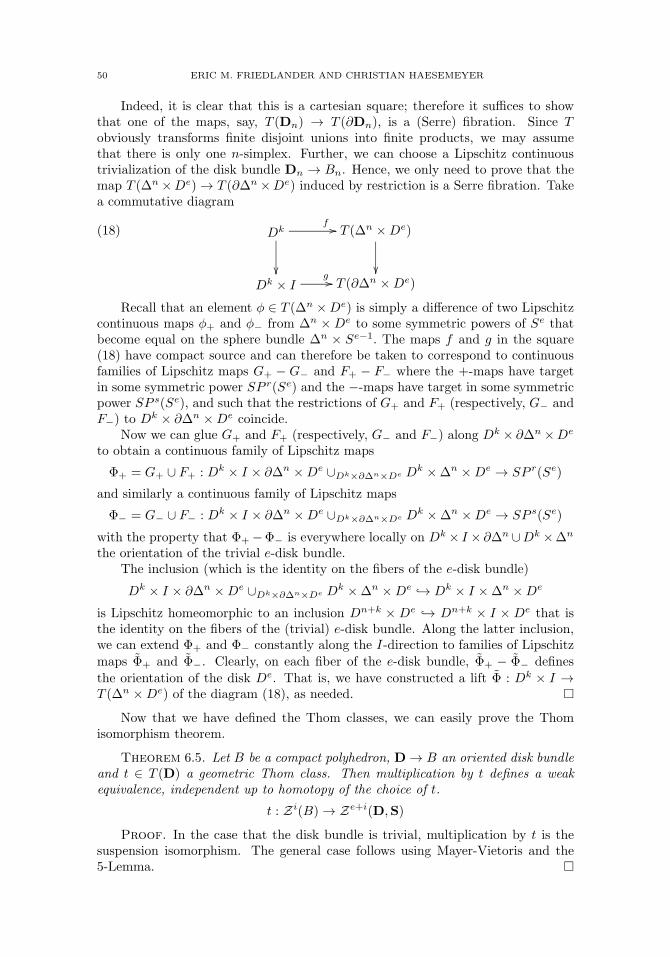
50 ERIC M. FRIEDLANDER AND CHRISTIAN HAESEMEYER
Indeed, it is clear that this is a cartesian square; therefore it suffices to showthat one of the maps, say, T (Dn) → T (∂Dn), is a (Serre) fibration. Since Tobviously transforms finite disjoint unions into finite products, we may assumethat there is only one n-simplex. Further, we can choose a Lipschitz continuoustrivialization of the disk bundle Dn → Bn. Hence, we only need to prove that themap T (Δn ×De) → T (∂Δn ×De) induced by restriction is a Serre fibration. Takea commutative diagram
(18) Dk
��
f �� T (Δn ×De)
��Dk × I
g �� T (∂Δn ×De)
Recall that an element φ ∈ T (Δn ×De) is simply a difference of two Lipschitzcontinuous maps φ+ and φ− from Δn ×De to some symmetric powers of Se thatbecome equal on the sphere bundle Δn × Se−1. The maps f and g in the square(18) have compact source and can therefore be taken to correspond to continuousfamilies of Lipschitz maps G+ − G− and F+ − F− where the +-maps have targetin some symmetric power SP r(Se) and the −-maps have target in some symmetricpower SP s(Se), and such that the restrictions of G+ and F+ (respectively, G− andF−) to Dk × ∂Δn ×De coincide.
Now we can glue G+ and F+ (respectively, G− and F−) along Dk × ∂Δn ×De
to obtain a continuous family of Lipschitz maps
Φ+ = G+ ∪ F+ : Dk × I × ∂Δn ×De ∪Dk×∂Δn×De Dk ×Δn ×De → SP r(Se)
and similarly a continuous family of Lipschitz maps
Φ− = G− ∪ F− : Dk × I × ∂Δn ×De ∪Dk×∂Δn×De Dk ×Δn ×De → SP s(Se)
with the property that Φ+ −Φ− is everywhere locally on Dk × I × ∂Δn ∪Dk ×Δn
the orientation of the trivial e-disk bundle.The inclusion (which is the identity on the fibers of the e-disk bundle)
Dk × I × ∂Δn ×De ∪Dk×∂Δn×De Dk ×Δn ×De ↪→ Dk × I ×Δn ×De
is Lipschitz homeomorphic to an inclusion Dn+k × De ↪→ Dn+k × I × De that isthe identity on the fibers of the (trivial) e-disk bundle. Along the latter inclusion,we can extend Φ+ and Φ− constantly along the I-direction to families of Lipschitz
maps Φ+ and Φ−. Clearly, on each fiber of the e-disk bundle, Φ+ − Φ− defines
the orientation of the disk De. That is, we have constructed a lift Φ : Dk × I →T (Δn ×De) of the diagram (18), as needed. �
Now that we have defined the Thom classes, we can easily prove the Thomisomorphism theorem.
Theorem 6.5. Let B be a compact polyhedron, D → B an oriented disk bundleand t ∈ T (D) a geometric Thom class. Then multiplication by t defines a weakequivalence, independent up to homotopy of the choice of t.
t : Zi(B) → Ze+i(D,S)
Proof. In the case that the disk bundle is trivial, multiplication by t is thesuspension isomorphism. The general case follows using Mayer-Vietoris and the5-Lemma. �

LIPSCHITZ COCYCLES AND POINCARE DUALITY 51
The following Thom Isomorphism theorem follows easily from Theorem 6.5.
Theorem 6.6. (Thom isomorphism) Let A be a compact polyhedron and C ⊂ Aa closed subpolyhedron of constant codimension e > 0 admitting an oriented normaldisk bundle in A (as in Proposition 6.1, for example). Then any geometric Thomclass t(C ⊂ A,Δ) determines a class τC ∈ Ze
C(A). Moreover, multiplication bysuch a class
τC : Zi(C) → Ze+iC (A)
is a weak equivalence, independent up to homotopy of the choice of τC .
Proof. The class tC = t(C ⊂ A,Δ) lies in the kernel of Ze(DΔ(C)) →Ze(SΔ(C)). Hence, we may extend tC by 0 on A − OΔ(C), obtaining the classτC in Ze(A) which vanishes off OΔ(C); in other words,
τC ∈ ker{Ze(A) → Ze(A−OΔ(C)} = ZC(A).
We now apply the excision property of Proposition 3.6 to identify the Thomisomorphism of Theorem 6.5 with multiplication by τC . �
References
[1] F. Almgren, Jr., Homotopy groups of the integral cycle groups. Topology 1 (1962), 257-299.[2] H. Federer, Geometric Measure Theory, Springer-Verlag, 1969.[3] E. Friedlander, Algebraic cocycles on normal, quasi-projective varieties, Compositio Math
110 (1998) 127-162.[4] E. Friedlander, Bloch-Ogus properties for topological cycle theory, Annales Ec. Norm sup. 33
(2000), 57-65.[5] E. Friedlander and H.B. Lawson, Duality relating spaces of algebraic cocycles and cycles,
Topology 36 (1997), 535 - 565.[6] E. Friedlander and H. B. Lawson, Graph mappings and Poincare Duality, Math. Ann. (2009),
431-461.[7] E. Friedlander and V. Voevodsky, Bivariant cycle homology in Cycles, Transfers, and Motivic
Homotopy Theories. Annals of Math Studies, pp. 138-183 (2000).[8] J.-H. Teh, Complexification of real cycles and the Lawson suspension theorem., J. Lond.
Math. Soc. 75 (2007), 463–478.
Department of Mathematics, University of Southern California, Los Angeles, CA
90089
E-mail address: [email protected]
Department of Mathematics, University of California, Los Angeles, CA 90095
E-mail address: [email protected]


Clay Mathematics ProceedingsVolume 9, 2010
On the motive of a K3 surface
Claudio Pedrini
1. Introduction
The existence of a suitable filtration for the Chow ring of every smooth projec-tive variety over a field k, as conjectured by Bloch and Beilinson has many importantconsequences both in arithmetic and in geometry. Apart from the trivial case ofcurves and some other particular cases, this conjecture is still wide open. Jannsenin [J1] has shown that the existence of a Bloch-Beilinson filtration F • for everysmooth projective variety is in turn equivalent to the existence of a Chow-Kunnethdecomposition as conjectured by Murre (see section 2).
In the case of surfaces a consequence of this Conjecture is Bloch’s Conjecture forsurfaces which asserts for a complex surface X that the action of a correspondenceΓ in X ×X on the graded group of 0-cycles of X only depends on the cohomologyclass of Γ. If X has geometric genus 0 this conjecture implies the converse toMumford’s famous necessary condition for the finite-dimensionality of the Chowgroup of 0-cycles (see [J1]). It is known for surfaces not of general type, for certaingeneralized Godeaux surfaces and in a few scattered cases. These conjectures areof motivic nature: in particular for a surface X with pg = 0, Bloch’s Conjecture isequivalent to the finite dimensionality of the motive of X (see [G-P]).The existence of a suitable Chow-Kunneth decomposition for the motive of a sur-face X shows that the information necessary to study the above Conjectures isconcentrated in the transcendental part of the motive t2(X) (see [KMP]).
According to Murre’s Conjecture (or equivalently to Bloch-Beilinson’s Conjec-ture) and to Kimura’s Conjecture on the finite dimensionality of motives (see [Ki])the following results should hold for a surface X:
(a) The motive t2(X) is evenly finite dimensional;(b) t2(X) satisfies the Nilpotency Conjecture (see 1.4);(c) Every homologically trival correspondence in CH2(X ×X)Q acts trivially
on the Albanese kernel T (X) (see 1.2);(d) The endomorphism group of t2(X) (tensored with Q) has finite rank (over
a field of characteristic 0).The motive t2(X) being a birational invariant vanishes for a rational surface.
Also (a) is known to hold for a Kummer surface X because t2(X) is isomorphic tot2(A), where A is an abelian surface (see [KMP 6.13]). Therefore, by the results in[Ki], also (b) holds for a Kummer surface.
c© 2010 Claudio Pedrini
53

54 CLAUDIO PEDRINI
A case where the above properties are still unknown is that of a K3 surfacewhich is not birational to a Kummer surface, in particular over C.
In this paper we analyze the relations between the statements in (a), (b) and(c) and prove some results for K3 surfaces. In particular in Theorem 5.10 weshow that, for a complex K3 surface X with a large Picard number ρ, the finitedimensionality of t2(X) implies the isomorphism of t2(X) with t2(Y ), where Yis a Kummer surface. On the other hand, if X and Y are complex distinct K3surfaces, which are general members of smooth projective families {Xt} and {Ys}over the disk Δ (hence ρ(X) = ρ(Y ) = 1), then Murre’s Conjecture implies thatHom(t2(X), t2(Y ) = 0 in the category of Chow Motives (Theorem 5.12).We also relate the Nilpotency Conjecture with Bloch’s Conjecture for complexsurfaces and extend a result by M. Saito in [MS] on the degree of nilpotency of ahomologically trivial correspondence (Theorem 3.6).
In section 2 we recall some known results on the category of Chow Motives and onthe different conjectures.Section 3 contains some properties about the Chow-Kunneth decomposition for themotive of a surface and the result on the degree of nilpotency.In section 4 we show how the transcendental motive of a surface varies in a smoothprojective family over a quasiprojective base. This is relevant in the case of K3surfaces because every complex projective K3 surface can be put in a smooth 1-dimensional family of K3 surfaces.Section 5 contains the results for complex K3 surfaces.In section 6 we consider the isomorphisms between the graded Chow ring of acomplex variety with the Deligne-Beilinson cohomology ring and collect some resultson the regulator map for complex K3 surfaces. We thank B. Kahn, L. Barbieri-
Viale, J. Murre, and C. Weibel for useful comments on a earlier draft of this paper.We also thank the Referee who suggested many improvements for the presentationof the paper.
2. Chow Motives, Bloch-Beilinson filtration and Murre’s Conjecture
Let X be a smooth projective variety over a field k. We will denote by Ai(X) =CHi(X)⊗Q the group of codimension i cycles on X modulo rational equivalencewith Q coefficients. Let Vk be the category of smooth projective varieties over k;by Mrat we will denote the (covariant) category of Chow motives over k. Objectsin Mrat are triples (X, p,m) where X = Xd is a d-dimensional smooth projectivevariety, p ∈ Ad(X ×X) is a projector, i.e.p2 = p, and m ∈ Z. Morphisms in Mrat
are defined as follows:
HomMrat((X, p,m), (Y, q, n)) = qCorrm−n(X,Y )p
where Corri(X,Y ) = Corr−i(Y,X) and
Corri(X,Y ) =⊕α
Adα+i(Xα × Y )
if X =∐
α Xα with Xα equidimensional of dimension dα. The covariant motivefunctor h : Vk → Mrat is defined as follows: h(X) = (X, 1X , 0) and h(f) = [Γf ] iff : X → Y . We give ourselves a Weil cohomology theory H∗ as defined in [Kl]: weshall denote its field of coefficients by K (by convention it is of characteristic 0). Foran element α ∈ Ai(X) we denote by clα its image under the cycle map Ai(X) →
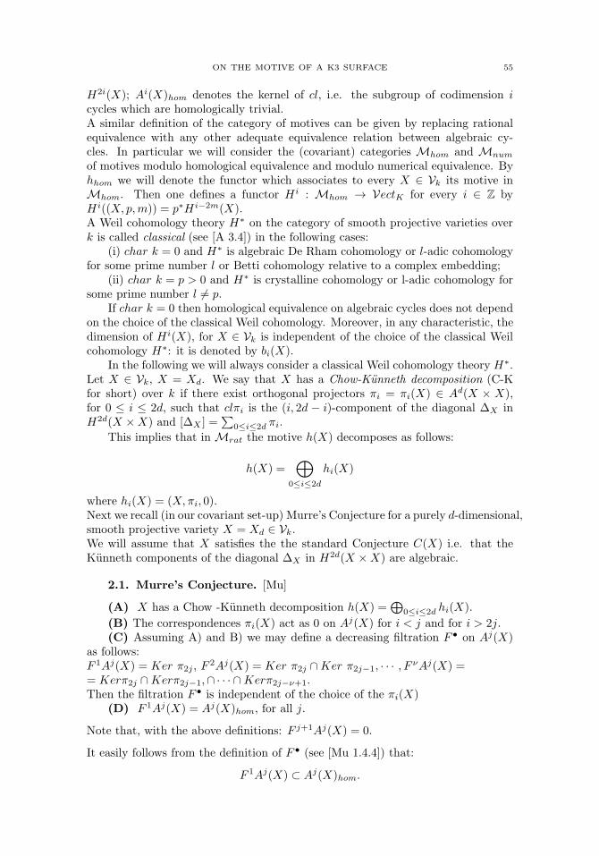
ON THE MOTIVE OF A K3 SURFACE 55
H2i(X); Ai(X)hom denotes the kernel of cl, i.e. the subgroup of codimension icycles which are homologically trivial.A similar definition of the category of motives can be given by replacing rationalequivalence with any other adequate equivalence relation between algebraic cy-cles. In particular we will consider the (covariant) categories Mhom and Mnum
of motives modulo homological equivalence and modulo numerical equivalence. Byhhom we will denote the functor which associates to every X ∈ Vk its motive inMhom. Then one defines a functor Hi : Mhom → VectK for every i ∈ Z byHi((X, p,m)) = p∗Hi−2m(X).A Weil cohomology theory H∗ on the category of smooth projective varieties overk is called classical (see [A 3.4]) in the following cases:
(i) char k = 0 and H∗ is algebraic De Rham cohomology or l-adic cohomologyfor some prime number l or Betti cohomology relative to a complex embedding;
(ii) char k = p > 0 and H∗ is crystalline cohomology or l-adic cohomology forsome prime number l �= p.
If char k = 0 then homological equivalence on algebraic cycles does not dependon the choice of the classical Weil cohomology. Moreover, in any characteristic, thedimension of Hi(X), for X ∈ Vk is independent of the choice of the classical Weilcohomology H∗: it is denoted by bi(X).
In the following we will always consider a classical Weil cohomology theory H∗.Let X ∈ Vk, X = Xd. We say that X has a Chow-Kunneth decomposition (C-Kfor short) over k if there exist orthogonal projectors πi = πi(X) ∈ Ad(X × X),for 0 ≤ i ≤ 2d, such that clπi is the (i, 2d − i)-component of the diagonal ΔX inH2d(X ×X) and [ΔX ] =
∑0≤i≤2d πi.
This implies that in Mrat the motive h(X) decomposes as follows:
h(X) =⊕
0≤i≤2d
hi(X)
where hi(X) = (X, πi, 0).Next we recall (in our covariant set-up) Murre’s Conjecture for a purely d-dimensional,smooth projective variety X = Xd ∈ Vk.We will assume that X satisfies the the standard Conjecture C(X) i.e. that theKunneth components of the diagonal ΔX in H2d(X ×X) are algebraic.
2.1. Murre’s Conjecture. [Mu]
(A) X has a Chow -Kunneth decomposition h(X) =⊕
0≤i≤2d hi(X).
(B) The correspondences πi(X) act as 0 on Aj(X) for i < j and for i > 2j.(C) Assuming A) and B) we may define a decreasing filtration F • on Aj(X)
as follows:F 1Aj(X) = Ker π2j , F
2Aj(X) = Ker π2j ∩Ker π2j−1, · · · , F νAj(X) == Kerπ2j ∩Kerπ2j−1,∩ · · · ∩Kerπ2j−ν+1.Then the filtration F • is independent of the choice of the πi(X)
(D) F 1Aj(X) = Aj(X)hom, for all j.
Note that, with the above definitions: F j+1Aj(X) = 0.
It easily follows from the definition of F • (see [Mu 1.4.4]) that:
F 1Aj(X) ⊂ Aj(X)hom.
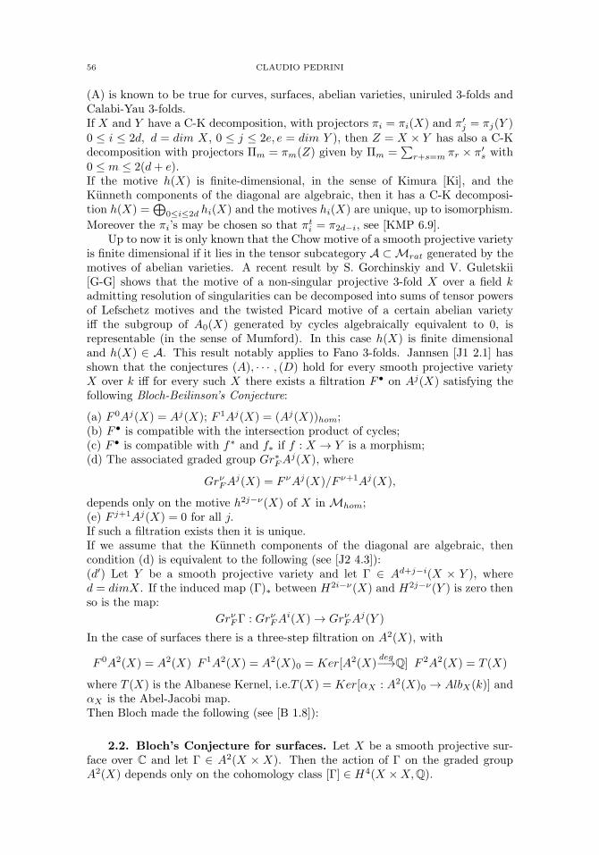
56 CLAUDIO PEDRINI
(A) is known to be true for curves, surfaces, abelian varieties, uniruled 3-folds andCalabi-Yau 3-folds.If X and Y have a C-K decomposition, with projectors πi = πi(X) and π′
j = πj(Y )0 ≤ i ≤ 2d, d = dim X, 0 ≤ j ≤ 2e, e = dim Y ), then Z = X × Y has also a C-Kdecomposition with projectors Πm = πm(Z) given by Πm =
∑r+s=m πr × π′
s with0 ≤ m ≤ 2(d+ e).If the motive h(X) is finite-dimensional, in the sense of Kimura [Ki], and theKunneth components of the diagonal are algebraic, then it has a C-K decomposi-tion h(X) =
⊕0≤i≤2d hi(X) and the motives hi(X) are unique, up to isomorphism.
Moreover the πi’s may be chosen so that πti = π2d−i, see [KMP 6.9].
Up to now it is only known that the Chow motive of a smooth projective varietyis finite dimensional if it lies in the tensor subcategory A ⊂ Mrat generated by themotives of abelian varieties. A recent result by S. Gorchinskiy and V. Guletskii[G-G] shows that the motive of a non-singular projective 3-fold X over a field kadmitting resolution of singularities can be decomposed into sums of tensor powersof Lefschetz motives and the twisted Picard motive of a certain abelian varietyiff the subgroup of A0(X) generated by cycles algebraically equivalent to 0, isrepresentable (in the sense of Mumford). In this case h(X) is finite dimensionaland h(X) ∈ A. This result notably applies to Fano 3-folds. Jannsen [J1 2.1] hasshown that the conjectures (A), · · · , (D) hold for every smooth projective varietyX over k iff for every such X there exists a filtration F • on Aj(X) satisfying thefollowing Bloch-Beilinson’s Conjecture:
(a) F 0Aj(X) = Aj(X); F 1Aj(X) = (Aj(X))hom;(b) F • is compatible with the intersection product of cycles;(c) F • is compatible with f∗ and f∗ if f : X → Y is a morphism;(d) The associated graded group Gr∗FA
j(X), where
GrνFAj(X) = F νAj(X)/F ν+1Aj(X),
depends only on the motive h2j−ν(X) of X in Mhom;(e) F j+1Aj(X) = 0 for all j.If such a filtration exists then it is unique.If we assume that the Kunneth components of the diagonal are algebraic, thencondition (d) is equivalent to the following (see [J2 4.3]):(d′) Let Y be a smooth projective variety and let Γ ∈ Ad+j−i(X × Y ), whered = dimX. If the induced map (Γ)∗ between H2i−ν(X) and H2j−ν(Y ) is zero thenso is the map:
GrνFΓ : GrνFAi(X) → GrνFA
j(Y )
In the case of surfaces there is a three-step filtration on A2(X), with
F 0A2(X) = A2(X) F 1A2(X) = A2(X)0 = Ker[A2(X)deg−→Q] F 2A2(X) = T (X)
where T (X) is the Albanese Kernel, i.e.T (X) = Ker[αX : A2(X)0 → AlbX(k)] andαX is the Abel-Jacobi map.Then Bloch made the following (see [B 1.8]):
2.2. Bloch’s Conjecture for surfaces. Let X be a smooth projective sur-face over C and let Γ ∈ A2(X × X). Then the action of Γ on the graded groupA2(X) depends only on the cohomology class [Γ] ∈ H4(X ×X,Q).
ON THE MOTIVE OF A K3 SURFACE 57
Now let X and Y be smooth projective varieties: the following result in [J1Prop. 5.8], relates Murre’s Conjecture for Z = X × Y , with the mophism groupsHomMrat
(hi(X), hj(Y )).
Proposition 2.1. Let X and Y be smooth projective varieties of dimensionsrespectively d and e, having a C-K decomposition and let Z = X × Y be providedwith the product C-K decomposition.
(1) If Z satisfies (B), then:
HomMrat(hi(X), hj(Y )) = 0 if j < i; 0 ≤ i ≤ 2d; 0 ≤ j ≤ 2e;
(2) If Z satisfies (D) then:
HomMrat(hi(X), hi(Y )) HomMhom
(hi,hom(X), hi,hom(Y )),
where hhom(X) =∑
0≤i≤2d hi,hom(X) and hhom(Y ) =∑
0≤j≤2e hj,hom(Y ) in Mhom.
In particular if X × X satisfies (D) and the field of coefficients of H∗ is K = Q
then (2) implies that the Q-vector space EndMrat(hi(X)), for 0 ≤ i ≤ 2d, has finite
dimension, being isomorphic to a sub-vector space of H∗(X ×X,Q).
Note that, because of our covariant definition of the functor h : Vk → Mrat, in (1)we have j < i, while in the contravariant setting (as in [J1 5.8]) one has i < j.
Remark 2.2. In the case dim X =dim Y =2 in [KMP 3.10] it has been provedthat (1) in Proposition 2.1 holds unconditionally for all i < j and 0 ≤ i ≤ 4, while(2) holds for all i �= 2. It follows that in Bloch’s Conjecture 1.2, the action ofa homologically trivial correspondence Γ on the components Q and AlbX of theChow group A0(X) vanishes. Hence the conjecture essentially reduces to the caseof the action of Γ on the Albanese kernel T (X).
Another conjecture, related to the previous ones is the following Nilpotency conjec-ture N(X).
2.3. Conjecture N(X). Let X = Xd be a smooth projetive variety over kof dimension d and let N (X) be the ideal in Ad(X ×X) of correspondences whichare numerically equivalent to 0. Then N (X) is a nilpotent ideal. In particular iff ∈ EndMrat
(h(X) is homologically trivial then f is nilpotent.
If the motive h(X) is finite dimensional then N(Xm) holds for all m ≥ 1 (see [Ki]).Also Murre’s Conjecture for X, X × X and X × X × X implies N(X) by [J1 p.294]. It follows that Murre’s Conjecture for all sufficiently high powers Xm impliesthe finite dimensionality of h(X) (having assumed C(X)).Kimura and O’Sullivan have conjectured (see [Ki]) that all smooth projective vari-eties have finite dimensional motives.The conjecture is known for curves and for some surfaces: rational surfaces, Godeauxsurfaces, Kummer surfaces, surfaces with pg = 0 which are not of general type, sur-faces isomorphic to a quotient (C ×D)/G, where C and D are curves and G is afinite group. It is also known for Fano 3-folds. In all these known cases the motiveh(X) lies in the tensor subcategory of Mrat generated by abelian varieties.By a result of V. Voevodsky [Voe1] (see also [Vois2]) if Γ ∈ Ad(X × X) is al-gebraically equivalent to 0 then it is smash nilpotent as an endomorphism inEndMrat
(h(X)). Therefore Γ is nilpotent (see [Ki 2.16]).

58 CLAUDIO PEDRINI
3. The refined Chow-Kunneth decomposition for a surface
If X is a smooth projective surface then there exists a refined Chow-Kunnethdecomposition of the motive h(X) with hi(X) = (X, πi, 0) in Mrat, as defined in[KMP 2.3], such that hi(X) are finite dimensional for i �= 2 and
EndMrat(hi(X)) EndMhom
(hhomi (X))
for i �= 2. Moreover π2 = πalg2 + πtr
2 and h2(X) = halg2 (X) + t2(X), where t2(X) =
(X, πtr2 , 0) and halg
2 (X) h(NSX)(1). Here h(NSX)is the Artin Motive associated
to NSX = NS(X ⊗k ks)Q for a separable closure ks of k. Then: A∗(halg2 (X)) =
A1(h2(X) = NS(X)Q and H2(X) = H2alg(X) ⊕ H2
tr(X) = (NS(X) ⊗ K) ⊕H2(t2(X), where K is the field of coefficients of H∗ and H2
tr(X) is the transcen-dental part of the cohomology. We also have the following equalities:
Hi(t2(X)) = 0 for i �= 2; H2(t2(X)) = πtr2 H2(X,Q) = H2
tr(X,Q),
Ai(t2(X)) = πtr2 Ai(X) = 0 for i �= 2; A0(t2(X)) = T (X),
where T (X) is the Albanese Kernel of X.From [KMP 4.3] we get, for X and Y surfaces
HomMrat(t2(X), t2(Y )) A2(X × Y )
J (X,Y )
where J (X,Y ) is the subgroup of A2(X × Y ) generated by the classes of corre-spondences which are not dominant over X and Y by either the first or the secondprojection.
The following theorem in [KMP 6.12] explains the relations between the tran-scendental part t2(X) of the motive of a surface and the different conjectures forh(X).
Theorem 3.1. Let X be a smooth projective surface and let
h(X) =⊕
0≤i≤4
hi(X) =⊕
0≤i≤4
(X, πi, 0)
be a refined Chow-Kunneth decomposition. Let us consider the following conditions:(1) the motive h(X) is finite-dimensional;(2) the motive t2(S) is evenly finite-dimensional;(3) every endomorphism f ∈ EndMrat
(h(S)) which is homologically trival isnilpotent, i.e. the conjecture N(X) holds;
(4) for every correspondence Γ ∈ A2(X × X)hom, αi,i = πi ◦ Γ ◦ πi = 0, for0 ≤ i ≤ 4;
(5) for all i, the map EndMrat(hi(X)) → EndMhom
(hi,hom(X)) is an isomor-phism (hence EndMrat
(hi(X)) has finite rank in characteristic 0);(6) the map EndMrat
(t2(X)) → EndMhom(thom2 (X)) is an isomorphism;
(7) A2(X ×X)hom ⊂ J (X).Then (1) ⇔ (2) ⇒ (3) ⇐ (4) ⇔ (5) ⇔ (6) ⇔ (7).
Note that, on the base of some conjectures on mixed motives, Beilinson haspredicted that for any smooth n-dimensional projective variety X, the Q-algebraAn(X×X)/J (X,X) is semisimple finite dimensional andAn(X×X)hom ⊂ J (X,X)(see [A 22.3.3]).
ON THE MOTIVE OF A K3 SURFACE 59
In the case of a complex surface X we also have the following result (see [KMP6.11]).
Theorem 3.2. Let X be a smooth projective surface over C. Then the followingconditions are equivalent:
(i) pg(X) = 0 and h(X) is finite dimensional;(ii) The Albanese Kernel T (X) vanishes;(iii) t2(X) = 0.
The following conjecture appears in [Vois1]. We will see how it is related withN(X).
3.1. Conjecture V(X). (see [Vois1 Conj. 6]). Let X be a surface: for everyΓ ∈ A2(X ×X)
Im F 2Γ∗ = Im F 2(Γ ◦ Γt)∗ ⊂ T (X)
where T (X) is the Albanese Kernel, and F 2Γ∗ denotes the action induced by Γ onT (X)
Remark 3.3. Let X,Y be complex varieties of dimension d and let Γ ∈ Ad(X×Y ). Then, by [Vois1 Lemma 5] there exists a morphism of Hodge structures
ψ : Hdtr(X,Q) → Hd
tr(Y,Q)
such that the action of Γ on Hdtr(X) is given by
[Γ]∗ = [Γ]∗ ◦ [Γt]∗ ◦ ψMoreover, if the Hodge conjecture is true, then ψ = Z∗, for some Z ∈ Ad(X × Y ).In particular, if dim X = dim Y = 2 then
Im [Γ ◦ Γt]∗ = Im[Γ]∗ ⊂ H2tr(Y )
and Ker[Γt]∗ = Ker[Γ ◦ Γt]∗.
Proposition 3.4. Let X be a complex surface. Assume Conjectures N(X) andV (X). Then X satisfies Bloch’s Conjecture 1.2.
Proof. Let Γ ∈ EndMrat(t2(X)) be homologous to 0. By V (X), in order
to compute the action of Γ on T (X) we may replace Γ by Γ ◦ Γt, hence we mayassume Γ is self-adjoint in A2(X ×X). By N(X) there exists n such that Γn = 0in A2(X × X), hence (F 2Γ∗)
n is 0 on T (X). Since Γ is self-adjoint, from V (X)it follows [Vois1 Remark 2] that Ker F 2Γ∗ = KerF 2(Γ ◦ Γ)∗ on T (X). ThereforeF 2Γ∗ is 0 on T (X). �
Example 3.5. [Vois1] Let X be a smooth projective surface which is fiberedover a 1-dimensional smooth basis S. Then every Γ ∈ A2(X ×S X) satisfies Con-jecture V (X).
By a result of M. Saito in [MS] the vanishing of T (X) for a complex surface Ximplies that the cube of the ideal:
A2(X ×X)hom = Ker(A2(X ×X) → H4(X ×X))

60 CLAUDIO PEDRINI
is 0. Note that, due to a result by Bloch and Srinivas in [B-Sr] if the Albanesekernel T (X) vanishes then there exist a divisor D on X and a subvariety V ⊂ Xof dimension ≤ 1 such that
ΔX = Γ1 + Γ2
where Γ1 is supported on D × X and Γ2 is supported on X × V . Therefore, ifT (X) = 0 every correspondence Z in A2(X × X) splits in Z1 + Z2, where Z1 issupported on D ×X and Z2 is supported on X × V .
Next Theorem generalizes M. Saito’s result.
Theorem 3.6. Let X be a smooth (irreducible) projective surface over a fieldk and let Ω be a universal domain containing k. Let Z be a homologically trivialcorrespondence in A2(X×X) such that F 2Z acts trivially on T (XΩ). Then Z3 = 0.
Proof. We have F 2Z = πtr2 ◦Z ◦πtr
2 . Let k(X) = k(ξ) be the field of fractionsof X, where ξ is the generic point of X. Choose an embedding k(X) ⊂ Ω. ThenF 2Z acts trivially on A0(Xk(X)) so that (πtr
2 ◦ Z ◦ πtr2 )(ξ) = 0. By [KMP 4.3] it
follows that Z = Z1 + Z2 where Z1, Z2 ∈ A2(X ×X), Z1 is supported on D ×Xand Z2 is supported on X × C with dim D ≤ 1 and dim C ≤ 1. By eventuallyconsidering the normalizations D and C we may also assume that both D and Care smooth.
Let h(X) =∑
0≤i≤4 hi(X) be a refined Chow-Kunneth decomposition as in
[KMP 2.3], where hi(X) = (X, πi, 0) are such that π0 = [X × P ], π4 = [P × X],and πi = πt
4−i. Here P is a rational point on X such that P /∈ D, P /∈ C. Inthe case X has no such rational point then one takes h0(X) = (X, π0, 0), whereπ0 = 1
n [X × P ], P a closed point on X with separable residue field k′ of degree n
over k (and similarly for π4). Moreover π2 = πalg2 + πtr
2 , h2(X) = halg2 (X) + t2(X)
where halg2 (X) = (X, πalg
2 , 0) h(NSX(1)), t2(X) = (X, πtr2 , 0) and h(NSX) is the
Artin motive associated to the Neron-Severi group NSX . Then A0(halg2 (X)) = 0
and A0(t2(X)) = T (X).We have Z = ΔX ◦ Z ◦ΔX =
∑i,j=0,...,4 πi ◦ Z ◦ πj . Since πi ◦ πj = 0 when i �= j
and πi ◦ πi = πi we get
Z3 =∑
h,i,j,k=0,...,4
πh ◦ Z ◦ πi ◦ Z ◦ πj ◦ Z ◦ πk
Since Z ∈ J(X) ∩A2(X ×X)hom from [KMP 3.10] and [KMP 4.5] we get
πj ◦ Z ◦ πi = 0
for j ≤ i and all i, j = 0, · · · , 4. Hence the sum above reduces to the strictlydecreasing sequences
Z3 = π4 ◦ Z ◦ π3 ◦ Z ◦ π2 ◦ Z ◦ π1 + π3 ◦ Z ◦ π2 ◦ Z ◦ π1 ◦ Z ◦ π0
To prove the claim it is sufficient to show that Z ◦ π0 = π4 ◦ Z = 0. By thechoice of π0 we have Z1 ◦π0 = 0, hence Z ◦π0 = Z2 ◦π0. Similarly π4 ◦Z = π4 ◦Z1
and so, passing to the transpose it suffices to show that Z2 ◦ π0 = 0. But
Z2 ∈ A1(X × C) = Hom(h(X), h(C)) = Hom(h(X)⊗ h(C),L)
HenceZ2 ◦ π0 ∈ Hom(1, h(C)) = Hom(h(C),L) = A1(C)

ON THE MOTIVE OF A K3 SURFACE 61
The cycle Z ◦ π0 = Z2 ◦ π0 is homologically trivial in A1(C), therefore it must be0. Hence Z3 = 0. �
Remarks 3.7. : 1) According to Bloch’s Conjecture for surfaces the actionof every homologically trivial correspondence on T (XΩ) should be trivial, if Ω isa universal domain containing the field k. This conjecture implies the converse ofMumford’s Theorem i.e. if H2(X,Ql(1)) is algebraic for some prime l �= charkthen the Abel-Jacobi map
αΩ : A2(XΩ)0 → AlbX(Ω)
is an isomorphism (see [J1 1.12]).2) From the proof of theorem 2.7 it follows that, if T (X) �= 0 and H1(X,Q) �= 0,then the correspondence (π2 ◦ Z) ◦ (π1 ◦ Z) may be non zero. Hence Z2 �= 0. Asimilar result appears in [MS 2.4], where an example is given of a complex surfaceX, with H1(X) �= 0, such that the square of the ideal A2(X ×X)hom is nonzero.
4. The Chow specialization map
Fix a ground field k and let S be a smooth irreducible quasi-projective varietyover k. For simplicity, we will assume that k is algebraically closed of characteristic0 and dim S = 1. Let η be the generic point of S, and let 0 be a distinguishedclosed point on S. By considering the localizations of S at η and at 0 we mayrestrict to the case where S = Spec R, R a regular local ring with residue field kand function field K = k(S).
For a scheme X smooth and proper over S there is a specialization map (see[Fu p. 399])
σ : A∗(Xη) → A∗(X0)
which is a ring homomorphism, i.e. it preserves the intersection product. HereXη and X0 are the fibers of X respectively over the generic point and the closedpoint of S, and A∗ is the graded Chow ring of algebraic cycles modulo rationalequivalence with Q coefficients.
If X → S is a smooth projective morphism, then the specialization map σ onChow groups is compatible with the specialization isomorphism in cohomology andwith the cycle map cl, thus yielding a commutative diagram (see [C-H p. 465])
Ai(Xη)σ−→ Ai(X0)⏐⏐�cl ⏐⏐�cl
H2i(Xη)�−→ H2i(X0)
We also recall the ’spreading out’ argument for a cycle Zη ∈ Ai(Xη × Xη) (see[C-H p. 489]): if Zη is a cycle on Xη ×Xη, where η is the generic point of S, thenone takes a neighborhood U ⊂ S of η and a cycle ZU on XU ×U XU such thatZU/η = Zη and let Z on X ×S X be its Zariski closure. There is a commutative
diagram: Ai−1(X0 ×X0)i∗ ��
Ai(X ×S X)j∗ ��
i!
��
Ai(Xη ×Xη)��0
Ai(X0 ×X0)

62 CLAUDIO PEDRINI
where the top row is exact, i and j are the inclusion maps of X0×X0 and Xη ×Xη
in X ×S X and i! is the Gysin homomorphism as defined in [Fu 6.2]. For everycycle Zη ∈ Ai(Xη ×Xη) the specialization map
σ : Ai(Xη ×Xη) → Ai(X0 ×X0)
can be defined as follows: σ(Zη) = i!(Z) where j∗(Z) = Zη and the result doesnot depend on the choice of the spread Z. The ambiguity in spreading a cycle inAi(Xη ×Xη) is given by cycles in in Ai−1(X0 ×X0).
Proposition 4.1. If X → S is a smooth projective morphism of relative dimen-sion d and {πi}, with 0 ≤ i ≤ 2d, is a set of orthogonal idempotents in Ad(Xη×Xη)lifting the Kunneth components of the diagonal ΔXη
, then {σ(πi)} have the same
property in Ad(X0 ×X0).
Proof. From the commutativity of j∗ and i! with proper pushforwards, flatpullbacks and intersection products ([Fu 20.3]) it follows that the specializationmap σ in (3) is compatible with the composition of correspondences. Using thefact that σ induces isomorphism in cohomology we get our result. �
Theorem 4.2. Let f : X → S be a smooth, projective family of surfaces overan algebraically closed field k of characteristic 0, with S smooth and dim S =1.Let X = Xη be the fiber of f over the generic point η of S and X0 the fiberover a closed point 0 of S. Let h(X) =
∑0≤i≤4 hi(X) be a refined Chow-Kunneth
decomposition with hi(X) = (X, πi(X), 0) and let h(X0) =∑
0≤i≤4 hi(X0) be the
corresponding decomposition in Mrat(k), with hi(X0) = (X0, σ(πi(X)), 0), induced
by the specialization map σ. Let π2(X) = πalg2 (X) + πtr
2 (X): then
σ(πtr2 (X)) = πtr
2 (X0)⊕ τ (X0) πalg(X0) = σ(πalg2 (X))⊕ τ (X0)
Here τ (X0) ∈ A2(X0 × X0) is a projector such that (X0, τ (X0), 0) A and A isthe direct sum of r = ρ(X0) − ρ(X) copies of the Lefschetz motive L, with ρ(X0)and ρ(X) the ranks of the Neron- Severi groups respectively of X0 and X.
Proof. Let h2(X) = halg2 (X)⊕ t2(X) where halg
2 (X) = (X, πalg2 (X), 0) and
halg2 (X) L⊕ρ(X).
Let [Di] be an orthogonal basis for NS(X)Q and let (D1)0, . . . , (Dn)0 be the Chowspecialization of the divisors Di in A1(X0). Since the Chow-specialization is anisomorphism on Weil cohomology, and since the intersection matrix is determinedon the cohomological level, we can complete the system {(D1)0, . . . , (Dn)0} to abasis in the Neron-Severi group of X0
(D1)0, . . . , (Dn)0 Hn+1, . . . , Hm
such that m = ρ(X0) ≥ n and
halg2 (X0) = A⊕B,
where the motive B is defined by the projector
πalg2 (X0) =
∑i
1
< [(D0))i], [(D0)i] >[(D0)i]⊗ [(D0)i] ∈ A2(X0 ×X0)
ON THE MOTIVE OF A K3 SURFACE 63
and the motive A is defined by the projector
τ (X0) =∑j
[Hj ×Hj ]
< [Hj ], [Hj ] >
for n+ 1 ≤ j ≤ m. Then, σ(π2(X)) = π2(X0), by Prop. 3. 1, σ(halg2 (X)) = B and
A L⊕r with r = m− n. Therefore
πalg2 (X0) = σ(πalg
2 (X)) + τ (X0); σ(πtr2 (X)) = τ (X0) + πtr
2 (X0)
�
Proposition 4.3. Let f : X → S be a smooth, projective family of surfacesover a field k of characteristic 0, where S is a geometric DVR of equicharacteristic0 with generic point η and closed point s. If t2(Xη) is finite dimensional then alsot2(Xs) is finite dimensional.
Proof. Let K be any field and let DMQ(K) be the triangulated category ofmotives as defined by V. Voevodsky in [Voev 2]. There is a fully faithful embedding
j : Mrat(K) → DMQ(K).
Let Ψ be the ”vanishing cycle functor” defined by J. Ayoub in [Ay 1.5]
Ψ : DM ctQ (k(η)) → DM ct
Q (k(s))
where, for a field K, DM ctQ (K) denotes the subcategory generated (up to twists
and taking direct factors) by the images, under the functor j, of the motivesh(X) ∈ Mrat(K). The functor Ψ is triangulated and tensor, hence Ψ(∧nh(X)) =∧nΨ(h(X), for all h(X) ∈ Mrat(k(η)). If t2(Xη) is finite dimensional, then itis evenly finite dimensional (see Theorem 3.1) so that ∧nt2(Xη) = 0 for some n.Therefore ∧nt2(Xs) = Ψ(∧nt2(Xη)) = 0. �
5. Complex K3 surfaces
In this paragraph we prove some results on the motive t2(X) for a complexK3 surface X. X is a regular surface (i.e. q(X) = 0), therefore it has refinedChow-Kunneth decomposition of the form h(X) =
∑0≤i≤4 hi(X) with h1(X) =
h3(X) = 0. Moreover h2(X) = halg2 (X) + t2(X), where t2(X) = (X, πtr
2 , 0) and
halg2 (X) L⊕ρ. Here ρ is the rank of the NS(X)Q = (PicX)Q so that 1 ≤ ρ ≤ 20.
Moreover
Hi(t2(X)) = 0 for i �= 2; H2(t2(X)) = πtr2 H2(X,Q) = H2
tr(X,Q),
Ai(t2(X)) = πtr2 Ai(X) = 0 for i �= 2; A0(t2(X)) = T (X),
where T (X) is the Albanese Kernel. Since q(X) = 0, we also have T (X) = A0(X)0(0-cycles of degree 0) and
dimH2(X) = b2(X) = 22 dimH2tr(X) = b2(X)− ρ
The family of K3 surfaces with Picard number ≥ ρ form a dense countable unionof subvarieties of dimension 20 − ρ in the family of all K3 surfaces. On a gen-eral K3 surface all divisors are linearly equivalent to some rational multiple of thehyperplane class, hence ρ = 1.

64 CLAUDIO PEDRINI
AK3 surface is called exceptional (or singular) if its Picard number ρ = dim Pic(X)Q= dim NS(X)Q = 20.For a Kummer surface, obtained by resolving the singularities of the quotient A/G,with A an abelian surface and G = {1,−1}, we have ρ ≥ 17.
Definition 5.1. A polarized complex K3 surface X is a K3 surface equippedwith an element α ∈ Pic X which is the class of an ample invertible sheaf. Asmooth family of K3 surfaces parametrized by a scheme S (over C) is a propersmooth morphism f : X → S whose fibers are K3 surfaces. A polarization of f isa section θ ∈ PicS X such that for any s ∈ S it is a polarization of Xs = f−1(s).Then R2f∗Z is a variation of Hodge structures on C; θ is at every point of type(1, 1) and its orthogonal P 2f∗Z is again a variation of Hodge structures (see [D6.3]).By a result of Deligne [D 6.4] for every complex polarized K3 surface X there existsa smooth family of polarized K3 surfaces {Xt}t∈Δ, where Δ is the unitary disk,such that the central fiber X0 is isomorphic to X.A complex K3 surface X will be said to be general if there exists a family {Xt}t∈Δ
such that X = Xt, where t belongs to the complement of a countable union ofanalytic subvarieties of Δ.
Remark 5.2. In [Ay 1.5.1] it has been conjectured that the functor Ψ, whichappears in Prop. 3. 3, is conservative, i.e. Ψ(A) = 0 implies A = 0. If this is thecase then every general K3 surface X will have finite dimensional motive. In factthere exists a smooth projective family of X → S such that X = Xt and the specialfiber Y = X0 is a Kummer surface. Therefore t2(Y ) is evenly finite dimensional i.e.∧nt2(Y ) = 0, for some n. Then Ψ(∧n(t2(X)) = ∧nt2(Y ) = 0, hence ∧nt2(X) = 0.
We will now show, using results in [P-S] and [K], that for a general K3 surfacethe image thom2 (X) of the transcendental motive t2(X) in the category Mhom(C) ofhomological motive is absolutely simple. It will follow that, for two distinct generalK3 surfaces X and Y
HomMhom(thom2 (X), thom2 (Y )) = 0
In Theorem 5.11 we will show that Murre’s Conjecture (D) implies
HomMrat(t2(X), t2(Y )) = 0.
Let’s consider the categoriesMrat(C) and Mhom(C) and letHSQ be the Tannakiancategory of Q-Hodge structures. ByHSGrQ we will denote the rigid tensor categoryof Z-graded objects of HSQ (see [A 7.1.2.1]). There is a Hodge realization functor
HHodge : Mrat(C) → HSGrQ
which factorizes trough Mhom(C). Let Mhom(C) be the subcategory generated bythe motives of all smooth projective varieties X satisfying the standard conjectureC(X), which amounts to the algebraicity of the Kunneth components of the di-
agonal in H∗(X × X). Mhom(C) contains all the motives of curves, surfaces andabelian varieties. Hhodge induces a functor
HHodge : Mhom(C) → HSQ
which is faithful.

ON THE MOTIVE OF A K3 SURFACE 65
Let X be a smooth complex projective surface, and let
h(X) =∑
0≤i≤4
hi(X)
be a refined Chow-Kunneth decomposition in Mrat(C), with h2(X) = halg2 (X) ⊕
t2(X). Let
hhom(X) =∑
0≤i≤4
hi,hom(X)
be the corresponding decomposition in Mhom(C). The maps
EndMrat(hi(X)) → EndMhom
(hi,hom(X)) ⊂ EndV ec(Q)(Hi(X))
are isomorphisms for i �= 2. Also halg2 (X) L⊕ρ, where ρ is the rank of the
Neron-Severi group, and EndMrat(L⊕ρ) EndMhom
(L⊕ρ). Therefore one has anisomorphism
h2,hom(X) = thom2 (X)⊕⊕α
Sα
where Sα L and 1 ≤ α ≤ ρ(X).Let f : X → S be a proper and smooth morphism of complex algebraic varieties.The Betti cohomology groups Hi(Xs) of the fibers Xs fit together into a localsystem which underlines a variation of Hodge structure V on S such that the Hodgestructure at s is just the Hodge structure on Hi(Xs). Therefore for every points ∈ S(C) there is a canonical action, i.e. the monodromy of π1(S(C), s) on H∗(Xs).Then we have the following
Proposition 5.3. Let S be a smooth complex variety. For a general s ∈ S(C)a finite index subgroup of the monodromy group is contained in the Mumford-Tategroup of the Hodge structure on Vs.
Proof. See [P-S Prop. 14]. �
From the result above we get (see [K 6.3]):
Theorem 5.4. Let X be a general complex K3 surface. Then the motivethom2 (X) is absolutely simple.
Proof. From [P-S Ex. 5 and Cor. 18] it follows that the Hodge realization ofthe motive thom2 (X) is absolutely simple. The functor HHodge being faithful we getthat thom2 (X) is also absolutely simple.
We recall from [AK 7] that, for an object M in a Q-linear, monoidal, rigid,symmetric, tensor category C such that End(1) = Q the trace tr(f) ∈ Q of amorphism f ∈ EndC(M) is defined by the composition
1η−→M∗ ⊗M
1⊗f−→M∗ ⊗MR−→M ⊗M∗ ε−→1
where ε is the evaluation map, η its dual and R is the switch.If f = idM then tr(idM ) = χ(M) is called the the Euler characteristic (or thedimension) of M .
The following example shows that for a Kummer surface the motive thom2 (X)may be not absolutely simple.
�

66 CLAUDIO PEDRINI
Example 5.5. Let A be a simple abelian surface over C ”having many endo-morphisms ” (or ”having complex multplication”, see [Mi]) i.e. such that
δ(M)d(M) = 4
where M = EndA⊗Q and δ, d are defined as follows:
δ(M) = [Z(M) : Q], d(M) = [M : Z(M)]1/2
with Z(M) the center of M (see [K 1.1]). Let X be the Kummer surface obtainedfrom A/G, where G =< 1,−1 >, by resolving singularities. Then t2(X) t2(A)(KMP 7. 6. 13]), so that also thom2 (X) thom2 (A). According to [K 5.2] one hasthom2 (X)⊗ Q = ⊕αSα with Sα simple, so that χ(Sα) = 1 and
∑α
χ(Sα) = b2 − ρ(X)
with b2 = 22 and ρ(X) ≤ 20. Hence the number of Sα is greater than 1. Let nτ bethe copies of Sτ appearing in the sum. Then
End(thom2 (X))⊗ Q End(⊕τ
nτSτ ) =∏τ
Mnτ(Q)
where Mnτis the ring of nτ by nτ matrices.
Definition 5.6. Let X and Y be two complex K3 surfaces. A Hodge cycleZ ∈ H4(X × Y,Q) is the sum of Zν ∈ (NS(X)⊗ NS(Y ))Q and Zτ ∈ (TX ⊗ TY ),where TX is the transcendental lattice H2
tr(X,Q) of X, and similarly for Y . AHodge cycle is algebraic iff so is Zτ . A Hodge cycle Z ∈ H4(X × Y,Q) is called aHodge isometry if it induces an isometry
Z∗ : H2tr(X,Q) → H2
tr(Y,Q)
which preserves the Hodge structures of H2tr(X)⊗ C and H2
tr(Y )⊗ C.
Proposition 5.7. Let X and Y be complex K3 surfaces and φ : H2tr(X) →
H2tr(Y ) a Hodge isometry. Then there exists an algebraic cycle Γ ∈ H4(X × Y,Q))
such that φ = Γ∗, where Γ∗ denotes the action of Γ on H∗(X). Moreover, ifρ(X) > 11 then there exists an isomorphism f : Y → X such that f∗ = φ onHtr
2 (X).
Proof. See [Muk Prop. 6.2] �
The following result can be viewed as an extension of Prop. 4. 7 to the case ofmotives.
Proposition 5.8. Let X and Y be complex K3 surfaces such that there existsan algebraic correspondence Γ ∈ A2(X × Y ) which induces an isomorphism Γ∗ :H2
tr(X) → H2tr(Y ). Assume that t2(Y ) is finite dimensional. Then t2(Y ) is a direct
summand of t2(X).
Proof. By Remark 2. 4 Im [Γ◦Γt]∗ = Im [Γ]∗ andKer [Γt]∗ = Ker [Γ◦Γt]∗ =0. Hence
[Γ ◦ Γt]∗ : H2tr(Y ) → H2
tr(Y )
ON THE MOTIVE OF A K3 SURFACE 67
is an isomorphism because H2tr(X) and H2
tr(Y ) are Q-vector spaces of the samedimension. The correspondence Z = Γ◦Γt yields a map between the transcendentalmotives
Z : t2(Y ) → t2(Y )
such that Zhom : thom2 (Y ) → thom2 (Y ) is an isomorphism in Mhom(C). Let A be thefull subcategory of Mrat(C) generated by evenly finite dimensional motives. Thent2(Y ) ∈ A and by [A-K 8.2.4] the functor Φ : A → A/N is conservative, i.e. itpreserves isomorphisms. Here N is the largest monoidal ideal in A distinct from A.The ideal N corresponds to numerical equivalence, hence Φ(Z) is an isomorphismin A/N . Therefore Z is an isomorphism in A. Let Z ′ be such that Z ′ ◦ Z = idt2(Y ).Then (Z ′ ◦ Γ) ◦ Γt = idt2(Y ) so that the map
Γt : t2(Y ) → t2(X)
is injective. Therefore t2(Y ) is a direct summand of t2(X). �
Definition 5.9. A Nikulin involution i on a K3 surface X is an involutionsuch that i∗(ω) = ω for all ω ∈ H2,0(X).
Theorem 5.10. Let X be a complex K3 surface and suppose that either ρ(X) =19, 20 or that ρ(X) = 17, 18 and there exists an embedding
TX ⊗Q ⊂ (U3 ⊗Q)
where U is a free Z-module of rank 2, whose bilinear form has matrix(0 11 0
)Then there exists a Kummer surface Y such that t2(Y ) is direct summand of t2(X).If t2(X) is finite dimensional then t2(X) t2(Y ).
Proof. By a result in [Mor pag. 121], which extends, using [Muk], a pre-vious one by [S-I] for ρ = 20, there exist an abelian surface A and an algebraiccorrespondence between X and A which induces a Hodge isometry between thetranscendental lattices TX and TA of X and A. Let Y be the Kummer surface as-sociated to A. Then there exists is a Nikulin involution i on X such that X/ < i >is birational to the Kummer surface Y . As in [Mor §3], by blowing up the 8 fixedpoints on X of the involution i, we have a diagram
X −→ X⏐⏐�g ⏐⏐�Y −→ X/ < i >
where Y X/G, G is the group generated by i and h(Y ) is finite dimensional,
because Y is birational to the Kummer surface Y . Moreover t2(X) = t2(X) becauset2(−) is a birational invariant for surfaces. Also
H2tr(X) H2
tr(X) H2tr(A) H2
tr(Y ).
Let p = 1/2(Γtg ◦ Γg) ∈ A2(X × X): then p is a projector and
h(X) = h((X, p))⊕ h((X,ΔX − p)) h(Y )⊕N
where N = h((X,ΔX − p). Hence t2(Y ) is a direct summand of t2(X).
68 CLAUDIO PEDRINI
If t2(X) is finite dimensional so it is h(X) and we are left to show that N = 0. The
map g induces an isomorphism on the cohomology groupsH∗(h(X)) and H∗(h(Y )),
because b2(X) = b2(Y ) = 22 and ρ(X) = ρ(Y ). Therefore the correspondenceΔX − p is homologically trivial. From [Ki] it follows that the projector ΔX − p isnilpotent, hence it is 0. Therefore we get N = 0. �
Remark 5.11. The following result by Nikulin in [N] has extended that ofMukai in Prop. 4. 7. The lattice of algebraic cycles SX of a K3 surface X is saidto represent 0 if there exists an element x ∈ SX such that x �= 0 and x2 = 0. Ifφ : TX ⊗Q TY ⊗Q is an isomorphism of the lattices of transcendental cycles oftwo K3 surfaces X and Y preserving the Hodge structure, then the cycle
Γφ ∈ (TX ⊗ TY )⊗Q ⊂ H4(X × Y,Q)
is algebraic iff SX represents 0, i.e. the surface X has a pencil of elliptic curves (inparticular this is so if rk SX ≥ 5).
Theorem 5.12. Let X and Y be distinct complex K3 surfaces which are generalmembers of smooth projective families X = {Xs}s∈S and Y = {Yt}t∈T , where Sand T are smooth quasiprojective varieties. Assume Murre’s Conjecture (D) forX × Y . Then
HomMrat(t2(X), t2(Y )) = 0
Consequently there exists no Hodge isometry between TX and TY .
Proof. By Proposition 2.1 the functor h : Mrat(C) → Mhom(C) induces anisomorphism
HomMrat(t2(X), t2(Y )) HomMhom
(thom2 (X), thom2 (Y ))
The variations of Hodge structures R2f∗Q and R2g∗Q corresponding to the familiesf : X → S and g : Y → T are distinct and simple. Since the Hodge realizationsHHodge is faithful it follows that
HomMrat(t2(X), t2(Y )) = 0.
Assume that there exists an isometry φ between the transcendental lattices TX
and TY . Then, by Prop 4. 7, φ is induced by an algebraic correspondence Γ ∈A2(X × Y ). The associated map
F 2Γ = πtr2 (Y ) ◦ Γ ◦ πtr
2 (X) ∈ HomMrat(t2(X), t2(Y ))
is 0. The mapφ = Γ∗ : TX = H2
tr(X) → TY = H2tr(Y )
also vanishes because π2tr(X) and π2
tr(Y ) act as the identity on H2tr. Therefore we
get a contradiction. �
Remark 5.13. In [C-L 2 3.2] it is proved that the existence of a Bloch-Beilinsonfiltration for X × Y , where X,Y are general K3 surfaces, implies
A2(X × Y ) =∑
0≤i≤2
Ai(X)⊗A2−i(Y )
ThereforeA2(X×Y ) = J (X,Y ), and this, by (1), impliesHomMrat(t2(X), t2(Y )) =
0.
ON THE MOTIVE OF A K3 SURFACE 69
6. Deligne-Beilinson’s Cohomology and the regulator map
Let A ⊂ C be a subring, which for us will be Z,Q or R: for every smoothalgebraic manifold Y over C, of dimension n, we will denote by Hi
D(Y,A(r)) theDeligne-Beilinson cohomology groups as defined in [E-V], where A(r) = (2πi)rA ⊂C. For A = Q and i = 2k−1 and Y smooth and projective there is an isomorphism
H2k−1D (Y,Q(k)) H2k−2(Y,C)
F kH2k−2(Y,C) +H2k−2(Y,Q(k)).
If A = R and we set
πk−1 : C = R(k)⊕ R(k − 1) → R(k − 1)
then
H2k−1D (Y,R(k)) H2k−2(Y,C)
F kH2k−2(Y,C) +H2k−2(Y,R(k))�−→
πk−1
Hk−1,k−1(Y,R)⊗ R(1) = Hk−1,k−1(Y,R(1))
where Hk−1,k−1(Y,R(1)) Hn−k+1,n−k+1(Y,R(n− k + 1))∨(see [C-L1]).Let Hp
D(A(r)) be the Zariski sheaves associated to Deligne-Beilinson cohomology,i.e. the sheaves on YZar associated to the presheaves
U → HpD(U,A(r)).
Similarly we will denote by Hp(A(r)) the Zariski sheaves associated to the sin-gular cohomology groups with A coefficients. The sheaf Hp
D(A(r)) has a Gerstenresolution
0 → HpD(A(r)) →
∐y∈Y 0
(iy)∗HpD(C(y), A(r)) →
∐y∈Y 1
(iy)∗Hp−1D (C(y), A(r−1)) → · · ·
where Y i is the set of points of codimension i in Y and
HiD(C(y), A(r)) = lim
U⊂{y}Hi
D(U,A(r)).
There is a coniveau spectral sequence
Ep,q2 = Hp(Y,Hq
D(A(r))) =⇒ Hp+qD (Y,A(r))
which gives an exact sequence of cohomology groups
0 → H1(Y,H2D(A(2)))
i→H3D(Y,A(2)))
ρ→H0(Y,H3D(A(2)))
δ→H2(Y,H2D(A(2))) → H4
D(Y,A(4))
For every U there is a natural map
ρU : O(U)∗alg → H1D(U,A(1))
which for A = Z is an isomorphism by [E-V 2.12]. From the Gersten reso-lution of the sheaf Hp
D(Q(r)) one gets a Bloch-Quillen isomorphism Ap(Y ) Hp(Y,Hp
D(Q(p))) (see [Gi]). This isomorphism yields an isomorphism of gradedrings
η : ⊕Ap(Y ) ⊕Hp(Y,HpD(Q(p)))
where the intersection product of algebraic cycles corresponds to the cup productin Deligne-Beilinson cohomology.

70 CLAUDIO PEDRINI
There are Chern class maps:
ci : Kp ⊗Q → H2i−pD (Q(i))
from the Zariski sheaf associated to K-theory to the Deligne-Beilinson cohomologysheaf. The kernel and cokernel of the Chern class c2 are constant sheaves (see [Ped]),hence c2 induces a surjective map H1(c2) : H1(Y,K2) ⊗ Q → H1(Y,H2
D(Q(2)).From the exact sequence in (4) we get for A = Q an exact sequence (see [BV 2])
0 → H1(Y,H2D(Q(2)))
i→H3D(Y,Q(2))
ρ→H0(Y,H3D(Q(2)))
δ→H2(Y,H2D(2)))
By composing the map H1(c2) with the inclusion H1(Y,H2D(Q(2))) ⊂ H3
D(Y,Q(2))one gets a map H1(Y,K2)⊗Q → H3
D(Y,Q(2))). The regulator map
c2,1 : CH2(Y, 1)Q → H3D(Y,Q(2))
is then defined using the isomorphism: H1(Y,K2) CH2(Y, 1) where CHk(Y,m)are Bloch’s Higher Chow groups. The map c2,1 can be explicitly described asfollows. A class ξ in H1(Y,K2) CH2(Y, 1) is represented by an element of theform ξ =
∑i(fi, Zi) where fi ∈ C(Zi)
∗, codim Zi = 1 and∑
i div fi = 0. Choose a
branch of the log function on C− [0,∞) and put γi = f−1i ([0,∞)), γ =
∑γi. Then
γ = δζ is a boundary. For ω ∈ F 1H2(Y,C) ⊂ H2(Y,C) one defines
c2,1(ξ)(ω) =1
(2πi)n−1(∑i
∫Zi−γi
ωlogfi + 2πi
∫ζ
ω)
The definition above gives a unique element in the quotient group
H3D(Y,Q(2)) H2(Y,C)
F 2H2(Y,C) +H2(Y,Q(2))
For any form ω ∈ Hn−1,n−1(Y,R(n− 1))∨ the real part of c2,1(ξ)(ω) is given by
1
(2πi)n−1(∑i
∫Zi
ωlog|fi|)
(see [C-L 1 p. 220]). The real regulator map
r2,1 : CH2(Y, 1) → H3D(Y,R(2)) H1,1(Y,R(1)) Hn−1,n−1(Y,R(n− 1))∨
is defined by
ξ =∑i
(fi, Zi) → r2,1(ξ)(ω) =1
(2πi)n−1(∑i
∫Zi
ωlog|fi|)
The following result has been proved by X. Chen and J. Lewis. Recall that, fora variety Y , a real analytic Zariski open set U in Y is the complement of a realanalytic subvariety of Y . If {Xt}t∈Y is a family of projective algebraic manifoldsthen X = Xt is said to be general if t ∈ U for some real analytic Zariski open setU .
Proposition 6.1. Let X be a smooth projective K3 surface over C which isgeneral. Then the real regulator r2,1 ⊗ R is surjective.
Proof. See [C-L1 1.1]. �Corollary 6.2. Let X be a K3 surface as in Proposition 6.1. Then the exact
sequence in (4) gives an isomorphism
H0(X,H3D(R(2))) = Ker [H2(X,H2
D(R(2))cl−→H4
D(X,R(2))]

ON THE MOTIVE OF A K3 SURFACE 71
Proof. By Proposition 6.1 the real regulator r2,1 is surjective, hence the group
H3D(X,R(2)) H1,1(X,R(1)) (H1,1(X,R(1)))∨
is generated by elements of the form
1
(2πi)n−1(∑i
∫Zi
ωlog|fi|)
with codimension Zi =1. Therefore, for every α ∈ H3D(X,R(2)), there is Zariski
open subset U ⊂ X such that α vanishes on U . The sheaf H3D(R(2)) has the
following resolution
0 → H3D(R(2)) → i∗(H
3D(C(X),R(2)) →
∐x∈X1
H2D(C(x),R(1)) → · · ·
where
H2D(C(x),R(1)) = lim
U⊂xH2
D(U,R(1)) = limU⊂xH1(U,C)
F 1H1 +H1(U,R(1))= 0
for x ∈ X1. The second equality comes from the vanishing of H2(U,R(1)) for U anaffine curve. The vanishing
limU⊂xH1(U,C)
F 1H1 +H1(U,Q(1))= 0
has been proved in[BV-S]. Therefore the resolution of the sheaf H3D(R(2)) gives an
isomorphism
H0(X,H3D(R(2))) H3
D(C(X),R(2)) = limU⊂XH3D(U,R(2))
limU⊂XH2(U,C)
F 2H2(U,C) +H2(U,R(2))
As we have seen for every α ∈ H3D(X,R(2)) there exists an open U ⊂ X such that
α vanishes in H3D(U,R(2)). It follows that the map ρ in the exact sequence coming
from (4)
H3D(X,R(2))
ρ→H0(X,H3D(R(2)))
δ→H2(X,H2D(R(2)))
cl→H4D(X,R(2))
is 0, so that
H0(X,H3D(R(2))) = Ker [H2(X,H2
D(R(2)))cl→H4
D(X,R(2))].
�
The following result, which appears in [Ros 6.1], shows that for a smooth pro-jective surface X over C the map
H0(X,H3D(X,Q(2)) → T (X) → 0
is an isomorphism iff pg(X) = 0. Here
T (X) = Ker [H2(X,H2D(Q(2)))
cl−→H4D(X,Q(2))]
is the Albanese Kernel. Therefore for a K3 surface the regulator
c2,1 : CH2(X, 1)Q → H3D(X,Q(2))
72 CLAUDIO PEDRINI
is not surjective because the map ρ in (6) is not 0.
Theorem 6.3. Let X be a smooth projective surface over C. Then there is anexact sequence
0 → H2(X,OX)
H2tr(X,Q) +G
→ H0(X,H3D(X,Q(2)) → T (X) → 0
The group G is at most countable.
Proof. By [Ros 6.1] there is an exact sequence
0 → H0(X,H2/F2,2Q ) → H0(X,H2(C)/F2H2)
H0(k22)−→ H0(X,H3D(Q(2))) → T (X) → 0
where F2,2Q = Image [H2
D(Q(2)) → H2(Q(2))] is the discrete part of the Deligne-
Beilinson cohomology sheaf. k22 is the map in the following exact sequence ofsheaves
0 → H2(Q)/F2,2Q → H2(C)/F2H2 k22
−→H3D(Q(2)) → 0
and F iHj are the Zariski sheaves associated to the presheaves U → F iHj(U,C).We also have
H0(X,H2/F2,2Q ) H1(X,F2,2
Q )⊕H0(X,H2(Q))
where H0(X,H2(Q)) H2tr(X,Q) and the group G = H1(X,F2,2
Q ) is at most
countable (see [Ped 1.7]). Finally, from [BV 2 §1], there is an isomorphism
H0(X,H2/F2H2) H2(X,OX).
�
Remarks 6.4. 1) For every smooth projective variety X over C there are exactsequences as in [Ped Th. 1.7]
0 → NS(X)⊗ C∗ → R(X) → H1(X,F2,2Z ) → 0
0 → H0(X,H2(Q/Z)) → H1(X,F2,2Z ) → H1(X,F2,2
Z )⊗Q → 0
where R(X) is the image of the regulator map c2,1 : H1(X,K2) → H3D(X,Z(2)),
F2,2Z is the image of H2
DZ(2)) in H2(Z(2)). The group (H1(X,F2,2Z ))tors is iso-
morphic to H0(X,H2(Q/Z)) (see [Ros 5.1]) and H1(X,F2,2Z ) ⊗ Q/Z = 0. Also
H1(X,F2,2)⊗Q is at most countable. The group H1(X,K2)⊗Q, which is isomor-phic to CH2(X, 1)Q, decomposes as follows ([Ped 1.10]):
H1(X,K2)⊗Q H1(X,F2,2Q )⊕ (NS(X)⊗ C∗)Q ⊕Ker(R(X))Q
For a surface X with pg(X) = 0 the regulator map c2,1 is surjective, becausethe map ρ in (6) is 0 by [BV 2 3.1]). Hence R(X)Q = H3
D(X,Q(2)) and T (X) =H0(X,H3
D(Q(2)). MoreoverH1(X,F2,2)⊗Q = 0, so thatH3D(X,Q(2)) = (NS(X)⊗
C∗)Q = NS(X)⊗ C/Q.

ON THE MOTIVE OF A K3 SURFACE 73
2) If X ⊂ P3 is a general hypersurface of degree d ≥ 5 then the regulatormap is not surjective because R(X)Q is contained in the image of H3
D(P3,Q(2)) →
H3D(X,Q(2)). More precisely: R(X)Q = NS(X)⊗C/Q C/Q and (H1(X,F2,2
Z )Q =0.
3) Let X be a surface of general type with pg(X) = 0. Then also q(X) =0 and Bloch’s Conjecture in 1.2 is equivalent to the vanishing of the AlbaneseKernel T (X). In fact the idempotent πtr
2 (X) which defines the summand t2(X) ofthe motive h(X) is in this case homologically trivial because H2
tr(X) = 0. FromTheorem 6.2 and the vanishing of H2(X,OX) we get the isomorphism
H0(X,H3D(Q(2))) T (X)
(see also [BV-Sr]). We also have H2(X × X,OX×X) = 0, hence by the results in[BV 2]
A2(X ×X)hom H0(X ×X,H3D(Q(2)).
Therefore Bloch’s Conjecture is equivalent to show that every element in H0(X ×X,H3
D(Q(2))) acts trivially on H0(X,H3D(Q(2)).
References
[A] Yves Andre pp. 1 - 260 Une introduction aux Motives 2004 Soc. Math. de France Panora-mas et Syntheses 17
[AK] Yves Andre and B. Kahn pp. 106-291 Nilpotence radicaux et structures monoidales (withan Appendix by P. O’sullivan) 2003 Rend. Sem. Mat Univ. Padova 108
[Ay] J. Ayoub pp. 3-54 The Motivic vanishing Cycles and the Conservation conjecture 2007”Algebraic Cycles and Motives” Vol 2, London Math. Soc. LNS 344, Cambridge UniversityPress
[BV1] L. Barbieri-Viale pp. 298-312 Balanced varieties 1999 Algebraic K-theory and its Appli-cations, World Scientific
[BV2] L. Barbieri-Viale pp. 298-312 On the Deligne -Beilinson cohomology sheaves 1994 Alg.Geom /9412006
[BV-S] L. Barbieri-Viale and V. Srinivas pp. 211-214 A reformulation of Bloch’s Conjecture 1995C. R. Acad. Sc. Paris 321 Serie I
[B] S. Bloch: Lectures on Algebraic Cycles Duke University Mathematics Series IV, DukeUniversity, Durham U.S.A. 1980
[B-Sr] S. Bloch and V. Srinivas pp. 1235-1253 Remarks on correspondences and algebraic cycles1983 Amer. J. of Math. 105
[C-H] A. Corti and M. Hanamura pp. 459-522 Motivic decomposition and intersection Chowgroups I 2000 Duke Math. J. 103, no. 3
[C-L1] X. Chen and J. Lewis pp. 213-240 The Hodge- D-Conjecture for K3 and Abelian Surfaces2005 Journal of Alg. Geom. 14
[C-L2] Xi Chen and J. Lewis pp. 271-283 The Real regulator for a product of K3 surfaces 2006AMS Studies in Adv. Math. Vol. 38
[D] P. Deligne pp. 137-252 La Conjecture de Weil pour les surfaces K3 1972 Inv. Math. 15[E-V] H. Esnault and E. Viehweg pp. 43-92 Deligne -Beilinson cohomology 1988 ”Beilinson’s
Conjectures on special values of L-functions”, Persp. Math. Vol. 4, Academic Press[FU] W. Fulton Intersection Theory Springer-Verlag Heidelberg- New-York 1984[Gi] H. Gillet pp. 285-288 Deligne homology and the Abel-Jacobi map 1983 Bull. AMS 10[G-G] S. Gorchinskiy and V. Guletskii pp. 1-21 Motives and representability of algebraic cycles
on threefolds over a field 2008 preprint[G-P] V. Guletskii and C. Pedrini pp. 243-263 Finite dimensional motives and the Conjectures
of Beilinson and Murre 2003 K-Theory 30[J1] U. Jannsen pp. 245-302Motivic Sheaves and Filtrations on Chow groups 1994 Proceedings
of Symposia in Pure mathematics Vol 55 Part. 1

74 CLAUDIO PEDRINI
[J2] U. Jannsen pp. 305-372 Deligne cohomology, Hodge D conjecture and motives 1988”Beilinson’s Conjectures on special values of L-functions”, Persp. Math. Vol. 4, AcademicPress
[K] B. Kahn pp. 1-69 Zeta functions and motives 2009 Pure and Applied Mthematics Quar-terly Vol 5, N. 1
[KMP] B. Kahn, J Murre and C. Pedrini pp. 1-58 On the transcendental part of the motiveof a surface 2007 ”Algebraic Cycles and Motives” Vol 2, London Math. Soc. LNS 344,
Cambridge University Press[Ki] S. I. Kimura pp. 173-201 Chow groups can be finite dimensional in some sense 2005 Math.
Ann. 331[Mi] J. Milne pp. 135-166 The Tate Conjecture for certain abelian varieties over finite fields
2001 Acta Arithmetica 100[Mor] D. R. Morrison pp. 105-121 On K3 surfaces with large Picard number 1984 Inv. Math. 75[Mu] J. Murre pp. 177-188 On a conjectural filtration on the Chow group of an algebraic variety
1993 Indag. Math. (N. S. ) 4 no. 2[Muk] S. Mukai pp. 341-413 On the moduli space of bundles of K3 surfaces 1 1987 Tata Inst. of
Fund. research Stud. math. 11 4 no. 2[MS] Morihiko Saito pp. 1-7 Bloch’s Conjecture and Chow Motives 2001 preprint[N] V. Nikulin pp. 375-383 On correspondences between K3 surfaces 1988 Math. USSR
Izvestyia Vol. 30 n. 2[Ped] C. Pedrini pp. 195-213 Bloch’s conjecture and the K-theory of projective surfaces 2000
CIRM Proceedings and Lecture Notes, Vol 24[P-S] C. Peters and M. Steenbrick pp. 183 -194 Monodromy of Variation of Hodge structures
2003 Acta Appl. Mathematicae 75[Ros] A. Rosenschon pp. 185-199 Indecomposable elements in K1 of a smooth projective variety
1999 K-Theory 16[S-I] T. Shioda and H. Inose pp. 119-136 On singular K3 Surfaces 1977 Complex Analysis and
Algebraic Geometry, Iwanami-Shoten, Tokyo[Voev1] V. Voevodsky pp. 187-198 A nilpotence theorem for cycles algebraically equivalent to 0
1995 Internat. Math. Res. Notices 4
[Voev2] V. Voevodsky pp. 188-238 Triangulated categories of motives over a field 2000 ”Cyclestransfers and motivic homology theories”, Ann. of Math. Stud. 143 Princeton Univ. Press
[Vois1] C. Voisin pp. 1-18 Remarks on filtrations on Chow groups and the Bloch Conjecture 2004Annali di Matematica
[Vois2] C. Voisin pp. 265-285 Remarks on zero cycles on self products of varieties 1996 Moduliof Vector Bundles, Lect. Notes in pure and apllied Math. 179, Dekker
Universita Degli Studi Di Genova, Dipartmento Di Mathematica, Via Dodecanesco,
35, 16146 Genova, Italy
E-mail address: [email protected]: http://www.dima.unige.it/~pedrini
Clay Mathematics ProceedingsVolume 9, 2010
Two observations about normal functions
Christian Schnell
Abstract. Two simple observations are made: (1) If the normal functionassociated to a Hodge class has a zero locus of positive dimension, then it hasa singularity. (2) The intersection cohomology of the dual variety contains thecohomology of the original variety, if the degree of the embedding is large.
This brief note contains two elementary observations about normal functionsand their singularities that arose from a conversation with G. Pearlstein. Through-out, X will be a smooth projective variety of dimension 2n, and ζ a primitive Hodgeclass of weight 2n on X, say with integer coefficients. We shall assume that X isembedded into projective space by a very ample divisor H, and let π : X → P bethe family of hyperplane sections for the embedding. The discriminant locus, whichparametrizes the singular hyperplane sections, will be denoted by X∨ ⊆ P ; on itscomplement, the map π is smooth.
1. The zero locus of a normal function
Here we show that if the zero locus of the normal function associated to a Hodgeclass ζ contains an algebraic curve, then the normal function must be singular atone of the points of intersection between X∨ and the closure of the curve.
Proposition 1. Let νζ be the normal function on P \ X∨, associated to anon-torsion primitive Hodge class ζ ∈ H2n(X,Z)∩Hn,n(X). Assume that the zerolocus of νζ contains an algebraic curve, and that H = dA for A very ample andd ≥ 3. Then νζ is singular at one of the points where the closure of the curve meetsX∨.
Before giving the proof, we briefly recall some definitions. In general, a normalfunction for a variation of Hodge structure of odd weight on a complex manifoldY0 has an associated cohomology class. If HZ is the local system underlying thevariation, then a normal function ν determines an extension of local systems
(1) 0 −−→ HZ −−→ H ′Z −−→ Z −−→ 0.
The cohomology class [ν] ∈ H1(Y0, HZ
)of the normal function is the image of
1 ∈ H0(Y0,Z
)under the connecting homomorphism for the extension.
2000 Mathematics Subject Classification. 14D05.Key words and phrases. Normal function, Singularity of normal function, Hodge conjecture,
Intersection cohomology, Dual variety.
c© 2010 Christian Schnell
75
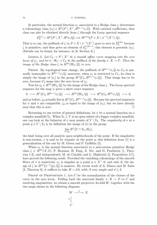
76 C. SCHNELL
In particular, the normal function νζ associated to a Hodge class ζ determinesa cohomology class [νζ ] ∈ H1
(P \X∨, R2n−1π∗Z
). With rational coefficients, that
class can also be obtained directly from ζ through the Leray spectral sequence
Ep,q2 = Hp
(P \X∨, Rqπ∗Q
)=⇒ Hp+q
(P ×X \ π−1(X∨),Q).
That is to say, the pullback of ζ to P ×X \ π−1(X∨) goes to zero in E0,2n2 because
ζ is primitive, and thus gives an element of E1,2n−12 ; this element is precisely [νζ ].
(Details can be found, for instance, in [6, Section 4].)
Lemma 2. Let C0 → P \ X∨ be a smooth affine curve mapping into the zerolocus of νζ , and let ψ : W0 → C0 be the pullback of the family π : X → P . Then theimage of the Hodge class ζ in H2n(W0,Q) is zero.
Proof. By topological base change, the pullback of R2n−1π∗Q to C0 is nat-urally isomorphic to R2n−1ψ∗Q; moreover, when νζ is restricted to C0, its class issimply the image of [νζ ] in the group H1
(C0, R
2n−1ψ∗Q). That image has to be
zero, because C0 maps into the zero locus of νζ .Now let ζ0 ∈ H2n
(W0,Q
)be the image of the Hodge class ζ. The Leray spectral
sequence for the map ψ gives a short exact sequence
0 −−→ H1(C0, R
2n−1ψ∗Q)−−→ H2n
(W0,Q
)−−→ H0
(C0, R
2nψ∗Q)−−→ 0,
and as before, ζ0 actually lies inH1(C0, R
2n−1ψ∗Q). Because the spectral sequences
for ψ and π are compatible, ζ0 is equal to the image of [νζ ]; but we have alreadyseen that this is zero. �
Returning to our review of general definitions, let ν be a normal function on acomplex manifold Y0. When Y0 ⊆ Y is an open subset of a bigger complex manifold,one can look at the behavior of ν near points of Y \ Y0. The singularity of ν at apoint y ∈ Y \ Y0 is by definition the image of [ν] in the group
limU�y
H1(U ∩ Y0, HZ
),
the limit being over all analytic open neighborhoods of the point. If the singularityis non-torsion, ν is said to be singular at the point y; this definition from [1] is ageneralization of the one by M. Green and P. Griffiths [5].
When νζ is the normal function associated to a non-torsion primitive Hodgeclass ζ ∈ H2n(X,Z), P. Brosnan, H. Fang, Z. Nie, and G. Pearlstein [1, Theo-rem 1.3], and independently M. de Cataldo and L. Migliorini [2, Proposition 3.7],have proved the following result: Provided the vanishing cohomology of the smoothfibers of π is nontrivial, νζ is singular at a point p ∈ X∨ if, and only if, the im-age of ζ in H2n
(π−1(p),Q
)is nonzero. By recent work of A. Dimca and M. Saito
[3, Theorem 6], it suffices to take H = dA, with A very ample and d ≥ 3.
Proof of Proposition 1. Let C be the normalization of the closure of thecurve in the zero locus. Pulling back the universal family π : X → P to C andresolving singularities, we obtain a smooth projective 2n-fold W , together with thetwo maps shown in the following diagram:
Wλ−−−−→ X
ψ
⏐⏐�C

TWO OBSERVATIONS 77
This may be done in such a way that the general fiber of ψ is a smooth hyperplanesection of X; let C0 ⊆ C be the open subset where this holds, and W0 = ψ−1(C0)its preimage. Assume in addition that, for each t ∈ C \ C0, the fiber Et = ψ−1(t)is a divisor with simple normal crossing support. The map λ is generically finite,and we let d be its degree.
Let ζW = λ∗(ζ) be the pullback of the Hodge class to W . By Lemma 2, therestriction of ζW to W0 is zero. Consider now the exact sequence
H2n(W,W0,Q)i−−→ H2n(W,Q) −−→ H2n(W0,Q).
By what we have just observed, ζW belongs to the image of the map i, say ζW =i(α). Under the nondegenerate pairing (given by Poincare duality)
H2n(W,W0,Q)⊗⊕
t∈C\C0
H2n(Et,Q) → Q,
and the intersection pairing on W , the map i is dual to the restriction map
H2n(W,Q) →⊕
t∈C\C0
H2n(EtQ),
and so we get that
d ·∫X
ζ ∪ ζ =
∫W
ζW ∪ ζW =⟨i(α), ζW
⟩=
∑t∈C\C0
⟨α, i∗t (ζW )
⟩where it : Et → W is the inclusion. But the first integral is nonzero, because theintersection pairing on X is definite on the subspace of primitive (n, n)-classes. Weconclude that the pullback of ζ to at least one of the Et has to be nonzero.
By construction, Et maps into one of the singular fibers of π, say to π−1(p),where p belongs to the intersection of X∨ with the closure of the curve. Thus ζ hasnonzero image in H2n
(π−1(p),Q
); by the result of [1, 2] mentioned above, νζ has
to be singular at p, concluding the proof. �I do not know whether a “converse” to Proposition 1 is true; that is to say,
whether the normal function associated to an algebraic cycle on X has to have azero locus of positive dimension for sufficiently ample H. If it was, this would giveone more equivalent formulation of the Hodge conjecture.
2. Cohomology of the discriminant locus
G. Pearlstein pointed out that the singularities of the discriminant locus shouldbe complicated enough to capture all the primitive cohomology of the originalvariety, once H = dA is a sufficiently big multiple of a very ample class. In thissection, we give an elementary proof of this fact for d ≥ 3.
To do this, we need a simple lemma, used to estimate the codimension of lociin X∨ where the fibers of π have a singular set of positive dimension. Let
Vd = H0(X,OX(dA)
)be the space of sections of dA, for A very ample.
Lemma 3. Let Z ⊆ X be a closed subvariety of positive dimension k > 0.Write Vd(Z) for the subspace of sections that vanish along Z. Then
codim(Vd(Z), Vd
)≥
(d+ k
k
).

78 C. SCHNELL
Proof. Since A is very ample, we may find (k + 1) points P0, P1, . . . , Pk onZ, together with (k + 1) sections s0, s1, . . . , sk ∈ V1, such that each si vanishes atall points Pj with j = i, but does not vanish at Pi. Then all the sections
s⊗i00 ⊗ s⊗i1
1 ⊗ · · · ⊗ s⊗ikk ∈ Vd,
for i0+ i1+ · · ·+ ik = d, are easily seen to be linearly independent on Z. The lowerbound on the codimension follows immediately. �
We now use this estimate to make the above idea about the cohomology of X∨
precise. As one further bit of notation, let Xsing ⊆ X stand for the union of all thesingular points in the fibers of π. It is well-known that Xsing is a projective spacebundle over X, and in particular smooth.
Proposition 4. Let H = dA for a very ample class A. If d ≥ 3, then the mapφ : Xsing → X∨ is a small resolution of singularities, and therefore
IH ∗(X∨,Q) � H∗(Xsing ,Q).
In particular, H∗(X,Q) is a direct summand of IH ∗(X∨,Q) once d ≥ 3.
Proof. By [3, p. Theorem 6], the discriminant locus is a divisor in P onced ≥ 3. This means that there are hyperplane sections of X with exactly oneordinary double point [8, p. 317]. The map φ is then birational, and therefore aresolution of singularities of X∨. To prove that it is a small resolution, take astratification of X∨ with smooth strata, and such the fibers of the map φ haveconstant dimension over each stratum; this is easily done, using the constructibilityof the higher direct image sheaves Rkφ∗Q.
Let S ⊆ X∨ be an arbitrary stratum along which the singular set of the fiberhas dimension k > 0. At a general point t ∈ S, there then has to be an irreduciblecomponent Z in the singular locus of pi−1(t) that remains singular to first orderalong S. Now a tangent vector to S may be represented by a section s of OX(dA),and a simple calculation in local coordinates shows that, in order for Z to remainsingular to first order, the section s has to vanish along Z. By Lemma 3, the spaceof such sections has codimension at least
(d+kk
), and a moment’s thought shows
that, therefore,
codim(S,X∨) ≥(d+ k
k
)− 1.
This quantity is evidently a lower bound for the codimension of the locus wherethe fibers of φ have dimension k. In order for φ to be a small resolution, it is thussufficient that (
d+ k
k
)− 1 > 2k
for all k > 0. Now one easily sees that this condition is satisfied provided thatd ≥ 3. This proves the first assertion; the second one is a general fact aboutintersection cohomology [4, pp. 120–1]. Finally, H∗(X,Q) is a direct summandof H∗(Xsing ,Q) because Xsing is a projective space bundle over X, and the thirdassertion follows. �
The proof shows that, as in the theorem by A. Dimca and M. Saito, d ≥ 2is sufficient in most cases. A result related to Proposition 4, and also showingthe effect of taking H sufficiently ample, was pointed out to me by H. Clemens;
TWO OBSERVATIONS 79
he noticed that, as a consequence of M. Nori’s connectivity theorem, one has anisomorphism
H2n(X,Q)prim � H1(P \X∨, (R2n−1π∗Q)van
),
once H is sufficiently ample [7, Corollary 4.4 on p. 364].
References
[1] P. Brosnan, H. Fang, Z. Nie, and G. Pearlstein, Singularities of admissible normal functions(2007), available at arXiv:0711.0964. To appear in Inventiones Mathematicae.
[2] M. A. A. de Cataldo and L. Migliorini, A remark on singularities of primitive cohomologyclasses (2007), available at arXiv:0711.1307v1. To appear in Proceedings of the A.M.S.
[3] A. Dimca and M. Saito, Vanishing cycle sheaves of one-parameter smoothings and quasi-semistable degenerations (2009), available at arXiv:0810.4896v2.
[4] M. Goresky and R. MacPherson, Intersection homology. II, Inventiones Mathematicae 72(1983), no. 1, 77–129.
[5] M. L. Green and P. Griffiths, Algebraic cycles and singularities of normal functions, Alge-braic cycles and motives (Grenoble, 2007), London Mathematical Society Lecture Note Series,vol. 343, Cambridge University Press, 2007, pp. 206–263.
[6] M. Saito,Hodge conjecture and mixed motives. I, Complex geometry and Lie theory (Sundance,UT, 1989), Proceedings of Symposia in Pure Mathematics, vol. 53, American MathematicalSociety, Providence, RI, 1991, pp. 283–303.
[7] M. V. Nori, Algebraic cycles and Hodge-theoretic connectivity, Inventiones Mathematicae 111(1993), no. 2, 349–373.
[8] C. Voisin, Theorie de Hodge et geometrie algebrique complexe, Cours Specialises, vol. 10,Societe Mathematique de France, Paris, 2002.
Department of Mathematics, Statistics & Computer Science, University of Illinois
at Chicago, 851 South Morgan Street, Chicago, IL 60607
E-mail address: [email protected]


Positive Characteristics andArithmetic


Clay Mathematics ProceedingsVolume 9, 2010
Autour de la conjecture de Tate a coefficients Z� pour lesvarietes sur les corps finis
Jean-Louis Colliot-Thelene et Tamas Szamuely
1. Introduction
Soient k un corps fini, k une cloture algebrique de k, G le groupe de GaloisGal (k|k) et � un nombre premier inversible dans k. Considerons une variete pro-jective, lisse, geometriquement integre X, de dimension d. D’apres la conjecture deTate, l’application cycle a valeurs dans la cohomologie etale �-adique induit unesurjection
(1) CHi(X)⊗Z Q� � H2i(X,Q�(i))G.
Une forme equivalente de la conjecture est la surjectivite du morphisme
(2) CHi(X)⊗Z Q� →⋃U
H2i(X,Q�(i))U
ou X := X ×k k et U parcourt le systeme des sous-groupes ouverts de G. La formeplus forte ci-dessus en resulte par un argument de restriction-corestriction.
On peut egalement considerer des formes entieres de ces enonces, et se demandersi les morphismes
(3) CHi(X)⊗Z Z� → H2i(X,Z�(i))G
ou
(4) CHi(X)⊗Z Z� →⋃U
H2i(X,Z�(i))U
induits par l’application cycle sont surjectifs. Ici le deuxieme enonce de surjectiviteest a priori plus faible.
Comme nous allons le rappeler dans la section 2, on ne s’attend pas a ce que lesformes entieres de la conjecture ci-dessus soient vraies. Neanmoins, il est raisonnabled’esperer la surjectivite de (3) et (4) pour i = d− 1, i.e. pour les 1-cycles.
Dans ce cas, la surjectivite de (4) a ete conditionnellement demontree par ChadSchoen :
c© 2010 Jean-Louis Colliot-Thelene et Tamas Szamuely
83

84 Jean-Louis Colliot-Thelene et Tamas Szamuely
Theoreme 1.1. (Schoen [15]) Soient k, G et X comme ci-dessus. Supposonsla conjecture de Tate connue pour les diviseurs sur une surface projective et lissesur un corps fini. Alors le morphisme
CH1(X)⊗ Z� →⋃U
H2d−2(X,Z�(d− 1))U
est surjectif, ou U parcourt le systeme des sous-groupes ouverts de G.
Notons que la conjecture de Tate pour les diviseurs sur une surface au-dessusd’un corps fini peut etre percue comme un analogue de la finitude hypothetique dugroupe de Tate-Shafarevich de la jacobienne d’une courbe sur un corps de nombres.
Nous expliquons la demonstration de Schoen (avec quelques modifications) dansles sections 3, 4 et 5.
Au paragraphe 6, on voit que le theoreme de Schoen a des consequences surl’existence de zero-cycles sur certaines varietes definies sur un corps de fonctionsd’une variable sur la cloture algebrique d’un corps fini. Voici un cas particulierconcret :
Corollaire 1.2. Soient k et X comme ci-dessus. Supposons qu’il existe unk-morphisme propre surjectif f : X → C, avec C une k-courbe propre lisse. Sup-posons en outre que la fibre generique de f est une intersection complete lisse dedimension ≥ 3 et de degre premier a car(k) dans un espace projectif, et que chacunedes fibres de f possede une composante de multiplicite 1. Si la conjecture de Tatepour les diviseurs sur les surfaces projectives lisses sur un corps fini est vraie, alorsle pgcd des degres des multisections de X → C est egal a 1.
2. Generalites sur la conjecture de Tate a coefficients entiers
On entend souvent dire : la conjecture de Hodge a coefficients entiers est fausse,il n’est pas raisonnable d’enoncer la conjecture de Tate avec des coefficients entiers.Quelle est la situation ?
Chacune de ces conjectures porte sur l’image d’une application cycle emanantdu groupe de Chow CHr(X) des cycles de codimension r sur une variete projectiveet lisse X de dimension d, a valeurs dans un groupe de cohomologie. Il s’agit deH2r(X,Z) pour Hodge et de H2r
et (X×kk,Z�(r)) pour Tate (dans cette section on vadistinguer les groupes de cohomologie etale des groupes de cohomologie singulierepar des indices pour ne pas induire une confusion). On trouvera dans le survol [23]de Voisin un etat des lieux pour la conjecture de Hodge.
Si l’on croit a ces conjectures a coefficients rationnels, la variante entiere peutetre mise en defaut de deux facons :
(a) on trouve une classe de cohomologie de torsion qui n’est pas la classe d’un cycle ;
(b) on trouve une classe de cohomologie d’ordre infini qui n’est pas dans l’image del’application cycle, mais qui donne un element de torsion dans son conoyau.
Pour la conjecture de Hodge entiere, il y a des contre-exemples de type (a) dusa Atiyah et Hirzebruch [1], reconsideres plus recemment par Totaro ([20], [21]),pour les groupes H2r(X,Z) avec r ≥ 2. L’exemple de dimension minimale chez euxest une variete de dimension 7, avec une classe de torsion dans H4(X,Z). Dansla litterature (par exemple dans Milne [10], Aside 1.4) il est affirme que l’on peutadapter ces exemples pour donner des contre-exemples a la conjecture de Tate

Autour de la conjecture de Tate a coefficients Z� 85
entiere sous la forme (4), mais a notre connaissance aucune demonstration n’a eteecrite. Voici donc une esquisse de demonstration qui met en relief les modifications afaire par rapport au cas analytique discute dans [1]. Il s’agit de prouver le theoremesuivant :
Theoreme 2.1.
(1) Soit V une variete projective et lisse sur un corps algebriquement clos.Pour tout � ≥ i inversible sur V les operations de Steenrod de degreimpair s’annulent sur la classe de tout cycle algebrique dans le groupeH2i
et (V,Z/�Z(i)).
(2) Au-dessus de tout corps algebriquement clos, pour tout premier � differentde la caracteristique, il existe une intersection complete lisse Y ⊂ PN ,un groupe fini G agissant librement sur Y , une classe c de �-torsion dansH4
et(Y/G,Z�(2)) et une operation de Steenrod de degre impair qui n’annulepas l’image de c dans H4
et(Y/G,Z/�Z(2)).
Ici pour � > 2 premier � operation de Steenrod de degre impair � veut direun compose d’operations de Steenrod Pj et d’une operation de Bockstein. Les
operations Pj : Hiet(V,Z/�Z) → H
i+2j(�−1)et (V,Z/�Z) en cohomologie etale ont
ete definies par Mme Raynaud dans [14]. Pour � = 2 on utilise des operations
Sqj : Hiet(V,Z/2Z) → Hi+j
et (V,Z/2Z), egalement definies dans [14].
Si le corps de base est une cloture algebrique F d’un sous-corps F , toute classede torsion dansH2i
et (V,Z�(i)) est invariante par un sous-groupe ouvert de Gal (F |F ),donc pour F fini le theoreme nous fournit un contre-exemple du type (a) a lasurjectivite des applications (3) et (4).
Esquissons une demonstration du theoreme qui nous a ete genereusement com-muniquee par Burt Totaro. Pour demontrer (1), la premiere observation est quepar le theoreme de Riemann-Roch sans denominateurs de Jouanolou ([5], Example15.3.6) pour � premier a (i − 1)! toute classe de cycle dans H2i
et (V,Z/�Z(i)) estcombinaison lineaire de classes de Chern ci(E) de fibres vectoriels E sur X. Il suffitdonc de demontrer l’enonce d’annulation pour les ci(E). Un calcul d’operations deSteenrod montre que l’annulation vaut pour E si et seulement si elle vaut pourE ⊗ L avec L tres ample de rang un. Ainsi, on peut supposer que E est engendrepar ses sections globales, et a fortiori qu’il est la tirette du fibre tautologique d’unegrassmannienne. L’enonce resulte alors de la fonctorialite contravariante des Pj
et de la trivialite de la cohomologie d’une grassmannienne en degres impairs ([8],expose VII, proposition 5.2).
Un point clef de l’argument d’Atiyah–Hirzebruch [1] etait l’identification dela cohomologie en bas degres d’une variete de Godeaux–Serre Y/G comme dans(2) a celle du produit d’espaces classifiants BG × BGm. On peut algebriser leurmethode en utilisant l’approximation algebrique de BG introduite par Totaro. Eneffet, d’apres ([21], Remark 1.4) pour tout s ≥ 0 il existe une representation k-lineaire W de G telle que l’action de G soit libre en dehors d’un ferme S de codi-mension s dans W . La cohomologie de BG := (W \ S)/G est egale a celle de Gjusqu’en degre s ; en particulier, elle ne depend ni du choix de W ni du choix deS. Le quotient P(W )//G := (P(W ) × (W \ S))/G est un fibre projectif sur BG,donc son anneau de cohomologie est un anneau de polynomes sur celui de BG. Enparticulier, la cohomologie de BG est facteur direct dans celle de P(W )//G.

86 Jean-Louis Colliot-Thelene et Tamas Szamuely
Si maintenant Y ⊂ P(W ) est une intersection complete lisse sur laquelle l’actionde G est libre, la cohomologie de Y/G est isomorphe a celle de P(W )//G en basdegres. En effet, la cohomologie de Y est isomorphe a celle de P(W ) jusqu’endegre dim (Y ) − 1 par le theoreme de Lefschetz faible. On en deduit un isomor-phisme entre les cohomologies de (Y × (W \ S))/G et de P(W )//G jusqu’en degredim (Y ) en appliquant la suite spectrale de Hochschild–Serre aux G-revetementsY × (W \ S) → (Y × (W \ S))/G et (P(W )× (W \ S)) → P(W )//G. Or la coho-mologie de (Y × (W \ S))/G s’identifie a celle de (Y ×W )/G jusqu’en degre s, etfinalement a celle de Y/G dans le meme intervalle, puisque W est un espace affine.
En somme, en bas degres la cohomologie de BG (donc celle de G) s’identifie aun facteur direct de celle de Y/G ci-dessus. La fin de la demonstration de (2) estalors similaire a celle de ([1], Proposition 6.7). Prenons G = (Z/�Z)3. Comme G estd’exposant �, la suite exacte longue associee a 0 → Z� → Z� → Z/�Z → 0 montreque Hi(G,Z�) s’identifie au noyau du morphisme de Bockstein β : Hi(G,Z/�Z) →Hi+1(G,Z/�Z). Le cup-produit des elements d’une base du (Z/�Z)-espace vectorielH1(G,Z/�Z) ∼= (Z/�Z)3 donne une classe dans H3(G,Z/�Z). Essentiellement lememe calcul que dans [1] montre que pour � > 2 l’image de cette classe dansH4(G,Z/�Z) par le Bockstein β n’est pas annulee par l’operation βP1, dont ledegre est 2�− 1. Pour � = 2 la meme conclusion vaut pour Sq3.
Terminons cette section par une breve discussion des contre-exemples de type (b).Un celebre contre-exemple de ce type a la conjecture de Hodge a ete fabrique parJ. Kollar [9] ; voir aussi [17]. Il s’agit d’une hypersurface � tres generale � dans P4
C
de degre m un multiple de �3 avec � entier premier a 6, et de l’application cycleCH2(X) → H4(X,Z). Comme il s’agit d’une hypersurface de degre m, ici on aH4(X,Z) ∼= Z, et l’image de l’application cycle contient mZ. Mais Kollar montrepar un argument de deformation astucieux que toute courbe sur X a un degredivisible par �. En d’autres mots, l’image de CH2(X) → H4(X,Z) est contenuedans �H4(X,Z) et ne peut etre surjective. Comme le note C. Voisin ([17], [23]),on peut a partir de cet exemple fabriquer des contre-exemples a la conjecture deHodge entiere en d’autres degres aussi, par eclatement ou par produit direct avecune autre variete.
L’enonce de Kollar en induit un au niveau de la cohomologie �-adique etale.En effet, si on travaille sur un corps algebriquement clos non denombrable et onchoisit � premier a la caracteristique et a 6, sa methode fournit toujours une hyper-surface X ⊂ P4 sur laquelle toute courbe a un degre divisible par �. (Le corps nondenombrable sert ici pour pouvoir choisir le point correspondant a X d’un schemade Hilbert convenable en dehors de la reunion d’une famille denombrable de fermespropres.) Ensuite, comme pour toute variete digne de ce nom, on trouve un corpsK de type fini sur le corps premier sur lequel X est definie. Notant K une cloturealgebrique de K, l’image de l’application cycle
CH2(X ×K K) → H4et(X ×K K,Z�(2)) ∼= Z�
est alors contenue dans �Z� ; noter qu’ici l’action de Galois sur la cohomologie induitl’action triviale sur Z�.
Remarques 2.2.
1. La methode ci-dessus ne permet pas de trouver un tel exemple avec K un corpsde nombres.

Autour de la conjecture de Tate a coefficients Z� 87
2. Par le theoreme 1.1, si on croit a la conjecture de Tate rationnelle pour lesdiviseurs sur les surfaces, en caracteristique positive le corps K ci-dessus ne peutetre un corps fini.
3. Nous ne savons pas s’il existe des contre-exemples du type (b) a la surjectivitede (3) sur un corps fini. En d’autres mots, nous ne savons pas si pour X projective,lisse, geometriquement connexe sur un corps fini k, l’application
CHi(X)⊗Z Z� → H2iet (X,Z�(i))
G/torsion
induite par l’application cycle est toujours surjective.Cette question est equivalente a la question suivante, fort interessante du point
de vue de [2] : pour tout i ≥ 0, l’application
CHi(X)⊗Z Z� → H2iet (X,Z�(i))/torsion
induite par l’application cycle
(5) CHi(X)⊗Z Z� → H2iet (X,Z�(i))
est-elle surjective ? Le lien entre les deux questions est fourni par les suites exactes
0 → H1(k,H2i−1et (Xk,Z�(i)))) → H2i
et (X,Z�(i)) → H2iet (Xk,Z�(i))
G → 0,
ou les groupesH1(k,H2i−1et (Xk,Z�(i)))) sont des groupes finis (ceci est une consequence
du theoreme de Deligne etablissant les conjectures de Weil).Notons ici pour usage ulterieur que par un argument bien connu utilisant la
suite de Kummer et le groupe de Brauer, pour i = 1 la surjectivite de (5) estequivalente a la conjecture de Tate a coefficients Q�, et meme a la bijectivite dumorphisme (1) (voir [19], Proposition 4.3). En vertu de la suite exacte ci-dessus,dans le cas des diviseurs la conjecture de Tate a coefficients Q� implique donc laversion entiere sous toutes ses formes possibles.
3. Le theoreme de Schoen, I : un argument de type Lefschetz
Nous commencons maintenant l’exposition de la demonstration du theoreme1.1, suivant [15].
Au cours de la preuve nous ferons a plusieurs reprises des extensions du corpsde base de degre premier a �. Un argument de restriction-corestriction fournit alorsle resultat au-dessus du corps de base initial.
Lemme 3.1. Il suffit d’etablir le theoreme 1.1 pour d = 3.
Demonstration. D’apres le theoreme de Bertini sur un corps fini [6, 13], onpeut trouver un plongement projectif de X et une hypersurface H tels que le k-schema Y = X∩H soit de codimension 1 dansX, lisse et geometriquement connexe.Comme X \Y est affine, pour d > 3, les theoremes sur la dimension cohomologiquedes schemas affines ([12], §VI.7) donnent
H2d−3(X \ Yk,Z�(d− 1)) = 0, H2d−2(X \ Yk,Z�(d− 1)) = 0.
Donc le morphisme compose
H2d−4(Yk,Z�(d− 2))∼→ H2d−2
Yk(X,Z�(d− 1)) → H2d−2(X,Z�(d− 1))
de l’isomorphisme de purete et de la fleche provenant de la suite de localisation estun isomorphisme (theoreme de Lefschetz faible, ibidem). Comme l’application cycleest compatible aux morphismes de Gysin ([12], Proposition VI.9.3), par recurrencesur d on se ramene donc au cas d = 3.
88 Jean-Louis Colliot-Thelene et Tamas Szamuely
Jusqu’a la fin du paragraphe 4, on suppose donc d = dim(X) = 3.
Remarquons ensuite qu’il suffit d’etablir le theoreme apres avoir eclate un pointde X, puisque la cohomologie de X s’identifie a un facteur direct de celle de l’eclate([4], expose XVIII, 2.2.2) et l’application cycle est compatible aux morphismespropres de varietes propres et lisses ([11], theoreme 6.1 et remarque 6.4). Ainsi,apres avoir fait un eclatement convenable, on peut tranquillement supposer que ledeuxieme nombre de Betti �-adique b2(X) de X est impair. En effet, si par malheurce nombre est pair, on eclate un point ferme de degre f impair (d’apres un argumentde type Lang–Weil, un tel point existe puisque la variete X est geometriquementintegre), ce qui donne pour l’eclate X∗ la formule b2(X
∗) = b2(X) + f d’apres [4],expose XVIII, (2.3.1). La raison pour cette hypothese supplementaire se devoileralors de la preuve de la proposition 3.3 ci-dessous.
Un calcul simple de classes de Chern (voir [16], 9.2.1) montre que, quitte acomposer le plongement projectif donne de X avec un plongement de Veronese dedegre pair, on peut supposer que le deuxieme nombre de Betti �-adique de toutesection hyperplane lisse de X est pair. Cette information de parite sera egalementimportante pour la suite.
Ayant fait une extension de degre premier a � si necessaire, on trouve un eclateV → X muni d’un pinceau de Lefschetz V → D ∼= P1 de sections hyperplanes ([4],
expose XVII, theoreme 2.5). Notons D ⊂ D le lieu au-dessus duquel le morphismeV → D est lisse, et choisissons un point generique geometrique ε de D. D’apres cequi precede, le deuxieme nombre de Betti de Vε est pair.
Introduisons les notations π (resp. π) pour le groupe fondamental arithmetique
(resp. geometrique) de D ayant ε pour point base.
Proposition 3.2. Quitte a faire une extension de k de degre premier a �, onpeut choisir le pinceau V de sorte que l’image de π dans AutZ�
(H2(Vε,Z�(1))) viala representation de monodromie soit infinie.
Demonstration. C’est la Proposition 1.1 de [15]. On ne donne que l’idee del’argument. Soit P l’espace projectif parametrisant les intersections de X avec leshypersurfaces de degre fixe suffisamment grand dans un plongement projectif fixe.Soient V ⊂ P×X l’hypersurface universelle, et P ⊂ P l’ouvert de lissite de la fibra-tion V → P. Le choix d’un pinceau de Lefschetz correspond au choix d’une droiteD ⊂ P, et on a V = V ×P D. Par un argument de type Bertini (voir par exemple[18], Lemma 5.7.2) apres une extension finie de k de degre premier a � on trouve D
assez generale pour laquelle l’homomorphisme π1(Dk, ε) → π1(Pk, ε) est surjectif. Ilsuffit donc de montrer que l’image du deuxieme groupe dans AutZ�
(H2(Vε,Z�(1)))est infinie. Schoen montre par une construction de geometrie algebrique classiquequ’il existe un autre espace projectif P et un morphisme P → P tels que le mor-phisme V×PP → P se factorise en V×PP → W → P , ou W est une hypersurfaceprojective lisse, et la dimension relative de W → P est 2. Comme W est une hy-persurface, elle se releve en caracteristique 0, et un theoreme de Deligne ([22],Theoreme B) montre que la monodromie de tout pinceau de Lefschetz balayant West infinie (sous l’hypothese car (k) �= 0 ; en caracteristique 2 un petit argumentsupplementaire est donne dans [15]). Ceci implique que la monodromie doit etreinfinie pour la fibration V×P P → P , et finalement pour V → P.

Autour de la conjecture de Tate a coefficients Z� 89
Expliquons maintenant l’idee de la preuve du theoreme 1.1. Tout d’abord,il suffit de montrer que toute classe dans H4(X,Z�(2))
G est la classe d’un cyclealgebrique sur X (ensuite, pour un sous-groupe ouvert U ⊂ G on peut appliquerce resultat apres changement de base de X au sous-corps fixe par U). Etant doncdonne w ∈ H4(X,Z�(2)) fixe par G, on montre qu’il est la poussette d’un element
de H2(Vx,Z�(1))Gal (k|k(x)), ou x est un point geometrique au-dessus d’un point
ferme x ∈ D. La conjecture de Tate pour les diviseurs sur la surface Vx (qui estvalable a coefficients Z� si elle est valable a coefficients Q� d’apres ce qu’on a ditdans la remarque 2.2 (3) ci-dessus) montre alors que cet element est la classe d’uncycle algebrique.
Notons qu’a coefficients Q� l’enonce voulu est une consequence directe dutheoreme de Lefschetz difficile (cf. la preuve du lemme 5.1 infra) ; toute la finessede l’argument consiste a en tirer un enonce a coefficients entiers.
Voici une reformulation. Ecrivons Xε pour le changement de base X ×Spec k ε.Par definition, il est muni de l’action triviale de π (celui-ci agissant sur les fibres dela fibration triviale X ×D → D), et par consequent
Hi(X,Z�(2))Gal (k|k) ∼= Hi(Xε,Z�(2))
π
pour tout i > 0. Notant Dx le groupe de decomposition d’un point x du revetementuniversel profini de D au-dessus de x, on obtient
Hi(Vx,Z�(2))Gal (k|k(x)) ∼= Hi(Vε,Z�(2))
Dx
pour tout i > 0 par le theoreme de changement de base propre et l’isomorphismeDx
∼= Gal (k|k(x)).Notons i l’inclusion de la surface Vε dans la variete Xε (qui est de dimension
3). Elle induit un morphisme de restriction
i∗ : H2(Xε,Z�(1)) → H2(Vε,Z�(1))
ainsi qu’une poussette
i∗ : H2(Vε,Z�(1)) → H4(Xε,Z�(2)).
D’apres la discussion ci-dessus, il suffit donc de montrer :
Proposition 3.3. Chaque element de H4(Xε,Z�(2))π est de la forme i∗(β),
avec un β ∈ H2(Vε,Z�(1)) invariant sous l’action d’un sous-groupe de decompositionDx dans π, pour un point x convenable.
Interrompons-nous pour quelques considerations d’algebre Z�-lineaire.
4. Le theoreme de Schoen, II : Lemmes d’algebre lineaire
Etant donnes un Z�-module B et un sous-ensemble A ⊂ B, on definit le satureAs de A dans B comme l’ensemble des b ∈ B avec �nb ∈ A pour un n ≥ 0convenable. On dit que A est sature dans B si As = A.
Lemme 4.1. Pour un module B de type fini sur Z� il existe un sous-groupeouvert Γ ⊂ AutZl
(B) tel que Bg soit sature dans B pour tout g ∈ Γ.

90 Jean-Louis Colliot-Thelene et Tamas Szamuely
Demonstration. Ecrire B = F ⊕ T avec F libre et T de torsion, et prendreΓ = AutZ�
(F )× {idT }.
Proposition 4.2. Soient F un Z�-module libre de rang fini impair, S ⊂ Fun sous-ensemble ouvert pour la topologie �-adique, et Φ : F × F → Z� une formebilineaire symetrique non degeneree sur Q�. Il existe alors un sous-ensemble ouvertS ⊂ O(F,Φ) tel que :
(a) chaque element de S admet un vecteur fixe non nul dans S ;(b) l’ouvert S contient des elements arbitrairement proches de 1 pour la topo-
logie �-adique.
Ici O(F,Φ) designe le groupe des automorphismes Z�-lineaires de F preservantΦ. Pour la preuve nous avons besoin d’un resultat ancillaire.
Lemme 4.3. Soient K un corps de caracteristique differente de 2, V un K-espacevectoriel de dimension finie impaire, et Φ une forme quadratique non degeneree surV . Tout element de SO(Φ) admet 1 comme valeur propre.
Demonstration. Notons A la matrice de Φ dans une base fixee de V . Pourun element de O(Φ) dont la matrice est M et la matrice transposee M t, on aM t.A.M = A. D’ou
M t.A.(M − I) = A−M t.A = (I −M t).A.
En prenant le determinant on obtient :
det(M). det(A). det(M − I) = det(I −M). det(A).
Ici det(A) �= 0 et det(M) = 1 (comme M ∈ SO(Φ)), donc det(M−I) = det(I−M).Comme V est de dimension impaire, ceci n’est possible que si det(M − I) = 0.
Demonstration de la proposition 4.2. Soit U ⊂ SO(FQ�,Φ) l’ouvert de Zariski forme
des elements ayant des valeurs propres distinctes. C’est aussi un ouvert de Zariskide O(FQ�
,Φ). Comme F est de rang impair, tout element de SO(FQ�,Φ) admet 1
comme valeur propre par le lemme 4.3. Donc tout u ∈ U stabilise un sous-espace Lu
de dimension 1 correspondant a la valeur propre 1. Envoyant u sur Lu on obtientune application continue λ : U → P(FQ�
). L’image de S \ 0 dans P(FQ�) par la
projection naturelle FQ�\ 0 → P(FQ�
) est ouverte, tout comme son image inverseS dans U ⊂ SO(FQ�
,Φ).Reste a voir que l’ensemble S est non vide, et qu’il contient des elements ar-
bitrairement proches de 1. Soit v ∈ S un vecteur non isotrope. Ecrivant FQ�=
〈v〉 ⊥ M avec un Q�-vectoriel M , on commence par montrer qu’il existe un elementde SO(M,Φ|M) a valeurs propres distinctes, et toutes differentes de 1. Pour cela, ondecompose l’espace quadratique M en une somme orthogonale d’espaces quadra-tiques Vi de dimension 2. Chaque SO(Vi) est un tore Ti = R1
ki/kGm de dimension 1,
ou ki/k est une algebre etale de degre 2 sur Q�. Si ki � Q� ×Q�, alors Ti � Gm,k,
et Gm,k agit sur Vi = Q� ⊕Q� par λ.(u, v) = (λ.u, λ−1.v). Si ki est une extensionquadratique de Q�, alors SO(Vi)(Q�) est le groupe des elements de norme 1 danski, et l’action de ce groupe sur Vi � ki est donnee par la multiplication dans ki.Les deux valeurs propres d’un element α ∈ SO(Vi)(Q�) ⊂ SO(Φ) ⊂ GL(V ) sontles conjugues de α (qui sont inverses l’un a l’autre). On trouve donc une familled’elements αi ∈ SO(Vi) dont la somme definit un element de SO(M,Φ|M) qui a des
Autour de la conjecture de Tate a coefficients Z� 91
valeurs propres distinctes et differentes de 1. De plus, on peut choisir les matricesdes αi de sorte qu’elles aient des coefficients dans Z� et qu’elles soient arbitraire-ment proches de la matrice 1 pour la topologie �-adique. Si elles sont suffisammentproches de 1, leur somme directe doit preserver la trace du reseau F sur M .
5. Le theoreme de Schoen, III : fin de la demonstration
Il nous reste a demontrer la proposition 3.3.
Lemme 5.1. Il existe une inclusion
H4(Xε,Z�(2))π ⊂ i∗((ker i∗ +Hπ)s),
ou
H := Im (i∗) ⊂ H2(Vε,Z�(1)).
Demonstration. Le morphisme compose
H2(Xε,Z�(1))i∗→ H2(Vε,Z�(1))
i∗→ H4(Xε,Z�(2))
est un isomorphisme apres tensorisation par Q� selon le theoreme de Lefschetzdifficile, car c’est le cup-produit par la classe de la section hyperplane Vε. Il estequivariant pour l’action de π, car Vε provient par changement de corps de based’une k(P1)-variete.
Donc par definition de H
i∗(Hπ)⊗Q�
∼= H4(Xε,Z�(2))π ⊗Q�,
d’ou
(6) H4(Xε,Z�(2))π ⊂ (i∗(H
π))s.
Remarquons maintenant que le morphisme
i∗ : H2(Vε,Z�(1)) → H4(Xε,Z�(2))
est surjectif. Ceci resulte du theoreme de Lefschetz faible : dans la suite de locali-sation
H4Vε(Xε,Z�(2)) → H4(Xε,Z�(2)) → H4(Xε \ Vε,Z�(2))
le dernier terme est 0, car la variete Xε \Vε est affine de dimension 3, et le premierterme est isomorphe a H2(Vε,Z�(1)) par purete.
En particulier, etant donne w ∈ H4(Xε,Z�(2))π, on trouve β ∈ H2(Vε,Z�(1))
avec
w = i∗(β).
D’autre part, (6) implique
�nw = i∗(γ)
pour un γ ∈ Hπ convenable et n ≥ 0. Mais comme �nw = i∗�nβ, on obtient
i∗(γ − �nβ) = 0, i.e. �nβ ∈ ker i∗ +Hπ, d’ou le lemme.
Corollaire 5.2. Pour w ∈ H4(Xε,Z�(2))π fixe, le sous-ensemble
Hw := {v ∈ ker i∗ : w ∈ i∗((v +Hπ)s)}de ker i∗ ⊂ H2(Vε,Z�(1)) est un ouvert non vide de ker i∗, stable par multiplicationpar �.
92 Jean-Louis Colliot-Thelene et Tamas Szamuely
Demonstration. Le lemme donneHw �= ∅ ; plus precisement, la preuve du lemmemontre que v0 := �nβ − γ ∈ Hw. Ce choix de n donne (v0 + �n ker i∗) ⊂ Hw, carpour δ ∈ ker i∗ et v = v0 + �nδ on a i∗(β + δ) = w et �n(β + δ) = v0 + �nδ + γ =v + γ ∈ (v + Hπ). Enfin, la stabilite de Hw par multiplication par � resulte de ladefinition.
Considerons maintenant la forme Z�-bilineaire sur H2(Vε,Z�(1)) induite par lecup-produit (i.e. la forme d’intersection) sur la cohomologie de la surface Vε, et no-
tons H⊥ l’orthogonal de H. On a alors ker i∗ ⊂ H⊥ ⊂ H2(Vε,Z�(1)), et l’inclusionker i∗ ⊂ H⊥ devient egalite apres tensorisation par Q�. En effet, les accouplementsde cup-produit satisfont a la compatibilite
α ∪ i∗(β) = i∗(α) ∪ β
pour α ∈ H2(Xε,Z�(2)) et β ∈ H2(Vε,Z�(1)), et ils sont non degeneres a coefficientsQ�.
Soit F ⊂ H⊥ un Z�-module libre, complement direct au sous-module de torsionT . Alors F ∩ ker i∗ est un sous-module ouvert dans F , et d’indice fini dans ker i∗.Ainsi le corollaire precedent implique :
Corollaire 5.3. Pour w ∈ H4(Xε,Z�(2))π fixe le sous-ensemble
Sw := {v ∈ ker i∗ ∩ F : w ∈ i∗((v +Hπ)s)}est un ouvert non vide de F .
Remarque 5.4. Quand X est une hypersurface dans P4, tous les Z�-modulesconsideres sont sans torsion, et l’on a ker i∗ = H⊥ = F , d’ou Hw = Sw.
Le lemme suivant distille la strategie de la demonstration de la proposition 3.3.
Lemme 5.5. Fixons w ∈ H4(Xε,Z�(2))π. Supposons qu’il existe g ∈ π satisfai-
sant aux trois hypotheses suivantes :
(1) H2(Vε,Z�(1))g est sature dans H2(Vε,Z�(1)) ;
(2) g engendre topologiquement le sous-groupe de decomposition Dx dans π ;
(3) g fixe un element v ∈ Sw.
Alors il existe β ∈ H2(Vε,Z�(1))Dx avec w = i∗(β).
Demonstration. Pour un v comme dans (3) on a (v + Hπ) ⊂ H2(Vε,Z�(1))g.
Comme H2(Vε,Z�(1))g est sature dans H2(Vε,Z�(1)), on a de plus (v + Hπ)s ⊂
H2(Vε,Z�(1))g = H2(Vε,Z�(1))
Dx . Mais par le corollaire precedent on a w = i∗(β)pour un β ∈ (v +Hπ)s.
Demonstration de la proposition 3.3. On cherche un g ∈ π satisfaisant aux condi-tions du lemme.
Par le theoreme de Lefschetz difficile, la restriction de la forme d’intersectionsurH2(Vε,Z�(1)) aH ⊗Q� est non degeneree (voir [3], Lemme 4.1.2). Sa restriction
a H⊥ ⊗ Q� est donc non degeneree. Ecrivant H⊥ = F ⊕ T comme ci-dessus, onpeut identifier O(F ) avec le stabilisateur (point par point) de T , qui est un sous-
groupe ouvert d’indice fini de O(H⊥). Comme l’image de π par la representation demonodromie ρ est infinie par construction (Proposition 3.2), un theoreme de Deligne([3], Theoreme 4.4.1) assure que c’est un sous-groupe ouvert de O(H⊥ ⊗ Q�). A

Autour de la conjecture de Tate a coefficients Z� 93
fortiori ρ(π)∩O(F ) est ouvert dans O(F ). Par le lemme 4.1 il existe un sous-groupeouvert G0 ⊂ ρ(π)∩O(F ) tel que H2(Vε,Z�(1))
g est sature dans H2(Vε,Z�(1)) pourtout g ∈ G0.
On applique maintenant la proposition 4.2 a F . Pour ce faire, on doit d’abordverifier que le rang de F est impair, i.e. que la dimension de H⊥ ⊗Q� est impair.Ceci resulte de nos hypotheses initiales que la dimension de H2(Vε,Q�(1)) est paireet celle de H2(Xε,Q�(1)) impaire ; on conclut par l’injectivite de i∗ ⊗ Q� (voir ledebut de la preuve du lemme 5.1). La proposition 4.2 (a) fournit donc un ouvert Sde O(F ) dont tout element a un vecteur fixe dans l’ouvert non vide Sw donne parle corollaire 5.3. De plus, la proposition 4.2 (b) assure que S contient des elementsarbitrairement proches de 1, donc son intersection avec le sous-groupe ouvert G0
est un ouvert non vide.L’image inverse de S ∩G0 dans π est un ouvert dont les elements satisfont aux
proprietes (1) et (3) du lemme ci-dessus. En outre, par definition de la topologie deπ elle contient une cosette hV d’un sous-groupe normal ouvert V ⊂ π. Appliquant letheoreme de densite de Tchebotarev au revetement galoisien Z → D correspondanta V on obtient un point ferme z ∈ Z dont le Frobenius associe dans π/V est h,
la classe de hV . Prenons alors un point x du revetement universel profini de Dau-dessus de z. Le sous-groupe de decomposition Dx est engendre par un element gd’image h dans π/V . Ceci veut dire que g est un element de hV , et en tant que telsatisfait aux hypotheses (1) et (3) du lemme. Par construction, il satisfait egalementa (2).
Remarque 5.6. Si l’on pouvait choisir V de telle sorte que le conoyau dumorphisme π/(V ∩π) → π/V soit d’ordre premier a �, alors une variante plus precisede l’argument de Tchebotarev ci-dessus donnerait un point ferme x de degre premiera �. L’existence d’un tel V impliquerait donc la conjecture de Tate a coefficients Z�
pour les 1-cycles sur X (en supposant la conjecture connue pour les surfaces).
6. Consequences du theoreme de Schoen
Nous donnons ici des applications du theoreme 1.1 a l’existence de zero-cyclesde degre premier a la caracteristique sur certaines varietes definies sur le corps desfonctions d’une courbe au-dessus de la cloture algebrique d’un corps fini. Il s’agitde deux enonces apparentes mais non equivalents dont chacun implique le corollaire1.2.
Theoreme 6.1. Soit k la cloture algebrique d’un corps fini k de caracteristiquep, et soit C une k-courbe propre lisse connexe, de corps des fonctions F = k(C).Fixons une cloture separable F de F .
Soit X une k-variete projective, lisse, connexe, admettant un k-morphisme pro-jectif et dominant f : X → C dont la fibre generique XF est lisse et geometriquementintegre.
Supposons :(i) Le groupe de Picard PicXF est sans torsion.(ii) Pour tout premier � different de p, la partie �-primaire du groupe de Brauer
BrX ⊂ BrXF est finie.(iii) La F -variete XF a des points dans tous les completes de F aux points
de C.

94 Jean-Louis Colliot-Thelene et Tamas Szamuely
(iv) Pour tout premier � different de p, la conjecture de Tate �-adique vaut pourles diviseurs sur les surfaces projectives et lisses sur un corps fini de caracteristiquep.
Alors XF possede un zero-cycle de degre une puissance de p.
Demonstration. Soit d + 1 la dimension de X, et donc d la dimension de laF -variete XF . Fixons une cloture separable F de F . Considerons la suite d’appli-cations
CHd(X)⊗ Z� → H2d(X,Z�(d)) → H2d(XF ,Z�(d)) → H2d(XF ,Z�(d)) ∼= Z�
La fleche H2d(X,Z�(d)) → H2d(XF ,Z�(d)) est obtenue par passage a la limite surles applications de restriction
H2d(X,Z�(d)) → H2d(X ×C U,Z�(d))
pour U parcourant les ouverts non vides de la courbe C. La compatibilite de l’ap-plication cycle a la restriction a un ouvert ([12], §VI, Prop. 9.2) montre que l’appli-cation composee ci-dessus se factorise a travers le groupe CHd(XF )⊗ Z�. Il suffitdonc d’etablir la surjectivite de l’application composee en question, pour tout �premier a p. On le fait en plusieurs etapes.
Surjectivite de CHd(X) ⊗ Z� → H2d(X,Z�(d)). Il existe un corps fini k ⊂ k etune k-variete X telle que X = X ×k k. La surjectivite requise resulte du theoreme1.1, pourvu qu’on demontre que tout element de H2d(X,Z�(d)) est fixe par unsous-groupe ouvert de Gal (k|k).
Or pour tout n > 0 la dualite de Poincare
H2d(X,μ⊗d�n ))×H2(X,μ�n) → Z/�nZ
est un accouplement parfait equivariant pour l’action de Galois. D’autre part, on ala suite exacte de Kummer
0 → PicX/�nPicX → H2(X,μ�n) → �nBrX → 0.
Le groupe PicX est extension du groupe de Neron-Severi NS(X) par le groupe�-divisible Pic 0 X. Le groupe NS(X) est de type fini, donc NS(X)/�n ∼= PicX/�n
est fixe par un sous-groupe ouvert de Gal (k|k) independant de n. Par l’hypothese(ii) le groupe �nBrX a egalement cette propriete. Il en est donc de meme pour le
groupe fini H2d(X,μ⊗d�n ), et a fortiori pour H2d(X,Z�(d)).
Surjectivite de H2d(X,Z�(d)) → H2d(XF ,Z�(d)). On va demontrer la surjectivite
de H2d(X,μ⊗d�n ) → H2d(XF , μ
⊗d�n ) pour tout n > 0. Ceci donnera un morphisme
surjectif de systemes projectifs de groupes abeliens finis, d’ou une surjection aprespassage a la limite projective suivant n.
On a la suite exacte de localisation
H2d(X,μ⊗dln ) → H2d(XF , μ
⊗dln ) →
⊕P∈C0
H2d+1
XP(X,μ⊗d
ln ),
ou P parcourt les points fermes de C. Montrons que chaque fleche H2d(XF , μ⊗dln ) →
H2d+1
XP(X,μ⊗d
ln ) est nulle. Pour ce faire, par excision on peut se restreindre au-dessus
du henselise R = OhC,P
de C en P , dont on note L le corps des fractions. On dispose
de la suite exacte de localisation
H2d(XR, μ⊗dln ) → H2d(XL, μ
⊗dln ) → H2d+1
XP(XR, μ
⊗dln ).

Autour de la conjecture de Tate a coefficients Z� 95
Il suffit donc d’etablir la surjectivite du morphismeH2d(XR, μ⊗d�n ) → H2d(XL, μ
⊗d�n ).
Le corps L est de dimension cohomologique 1 (c’est un corps C1). La suitespectrale de Hochschild–Serre donne donc naissance a la suite exacte courte
0 → H1(L,H2d−1(XL, μ⊗d�n )) → H2d(XL, μ
⊗d�n ) → H2d(XL, μ
⊗d�n )Gal (L|L) → 0.
D’autre part, le groupe H2d−1(XL, μ⊗d�n ) est dual de H1(XL, μ�n) ∼= �nPicXL par
dualite de Poincare. La torsion dans le groupe de Picard ne change pas par extensionde corps algebriquement clos, donc ce dernier groupe est nul par l’hypothese (i).Ceci donne des isomorphismes de modules galoisiens
H2d(XL, μ⊗d�n )) ∼= H2d(XL, μ
⊗d�n ) ∼= Z/�nZ.
L’hypothese queXF possede des points dans tous les completes de F est equivalentea la meme hypothese avec les henselises, d’ou en particulier une section du mor-phisme XR → SpecR par proprete de X. Elle donne naissance a un 1-cycle surXR dont la classe de cohomologie dans H2d(XR, μ
⊗d�n ) s’envoie sur le generateur de
H2d(XL, μ⊗d�n ).
Surjectivite de H2d(XF ,Z�(d)) → H2d(XF ,Z�(d)). Ici encore, il suffit d’etablirla surjectivite a niveau fini, car il resulte de l’etape precedente que les groupesH2d(XF , μ
⊗d�n ) sont finis. Le corps F est de dimension cohomologique 1, donc le
morphisme
H2d(XF , μ⊗d�n ) → H2d(XF , μ
⊗d�n )Gal (F |F )
dans la suite spectrale de Hochschild–Serre est une surjection. On aH2d(XF , μ⊗d�n ) ∼=
Z/�nZ avec action triviale de Galois, d’ou la surjectivite requise.
Une consequence facile du theoreme est le corollaire 1.2 de l’introduction.
Demonstration du corollaire 1.2. Comme le degre de la fibre generique du mor-phisme X → C est suppose premier a p, il suffit de montrer que les hypotheses (i)et (ii) du theoreme 6.1 sont satisfaites. En d’autre termes, on doit verifier que pourXF une intersection complete lisse de dimension ≥ 3 dans Pn
Fle groupe de Picard
est sans torsion �-primaire et la partie �-primaire du groupe de Brauer est finie.Le premier enonce resulte du theoreme de Noether–Lefschetz ([7], expose XII,
corollaire 3.7) : la fleche de restriction Z = PicPnF→ PicXF est un isomorphisme.
D’autre part, la suite exacte de Kummer en cohomologie etale donne une suiteexacte
0 → PicXF /�PicXF → H2(XF ,Z/�Z) → �BrXF → 0.
On vient de voir que le premier terme est isomorphe a Z/�Z. Mais ceci vautegalement pour le deuxieme, car il est isomorphe a H2(Pn
F,Z/�Z) par le theoreme
de Lefschetz faible en cohomologie etale. On constate donc avec satisfaction que ledernier terme disparait, ce qui montre que la partie �-primaire de BrXF est en faittriviale.
Le corollaire 1.2 peut egalement se deduire du theoreme 6.2 ci-apres. Il s’agitd’une variante du theoreme 6.1, avec la difference sensible qu’ici on fait une hy-pothese au-dessus du corps de fonctions d’une courbe definie sur un corps fini, etnon pas sur Fp.
Soient donc C une courbe propre, lisse, geometriquement connexe definie surun corps fini k, et Y une variete lisse sur le corps des fonctions k(C) de C. Pour

96 Jean-Louis Colliot-Thelene et Tamas Szamuely
un point ferme P de C notons KP le complete de k(C) pour la valuation discreteassociee a P . Une famille {zP } de zero-cycles de degre 1 sur Y ×k(C) KP pour toutP definit un homomorphisme BrY → Q/Z donne par A �→ ΣP invP (A[zP ]). IciBrY est le groupe de Brauer de Y , le morphisme invP est l’invariant de Hasse ducorps local KP , et A[zP ] est l’evaluation de l’element A ∈ BrY en zP definie via lafonctorialite contravariante du groupe de Brauer.
On dit qu’il n’y a pas d’obstruction de Brauer–Manin a l’existence d’un zero-cycle de degre 1 sur Y s’il existe une famille {zP } pour laquelle l’homomorphismeci-dessus est nul. Notons que cette condition est automatique si la fleche naturelleBr k(C) → BrY est surjective.
Theoreme 6.2. Soient k un corps fini de caracteristique p, et X → C unmorphisme projectif et dominant de k-varietes projectives lisses geometriquementconnexes, ou C est une courbe et la fibre generique Xk(C) est lisse et geometrique-ment integre.
Supposons :(i) Il n’y a pas d’obstruction de Brauer–Manin a l’existence d’un zero-cycle de
degre 1 sur la k(C)-variete Xk(C).(ii) La conjecture de Tate sur les diviseurs vaut sur les surfaces projectives et
lisses sur un corps fini.Alors la k(C)-variete X×k(C)k(C) possede un zero-cycle de degre une puissance
de p.
Demonstration. Soit d + 1 la dimension de X, et donc d la dimension de lak(C)-variete Xk(C). Soit � �= p un nombre premier, et soit {zP } une famille de zero-cycles de degre 1 sur les X ×k(C) KP pour laquelle l’application BrXk(C) → Q/Zdefinie ci-dessus est nulle. La proposition 3.1 de [2] fournit alors un element z de
H2d(X,Z�(d)) dont la restriction dans le groupe H2d(X ×k(C) k(C),Z�(d)) � Z�
est egale a 1 ∈ Z�. D’apres le theoreme 1.1, l’image de z dans H2d(X ×k k,Z�(d))provient d’un element Z de CH1(X×k k)⊗Z�. Prenant la trace de Z dans le groupeCH0(X ×k(C) k(C))⊗ Z� on voit que le morphisme CH0(X ×k(C) k(C)) → Z/�Zinduit par le degre est surjectif.
Remarque 6.3. La demonstration de la proposition 3.1 de [2] invoquee ci-dessus utilise des arguments voisins de ceux rencontres dans la preuve du theoreme6.1. Une difference notable est que, dans la notation de ladite preuve, l’existence declasses de cohomologie de degre 1 sur les schemas XR implique directement l’exis-tence d’une classe globale de degre 1 sur X grace a l’hypothese � arithmetique �detype Brauer–Manin, sans imposer une hypothese geometrique comme l’hypothese(i) du theoreme 6.1.
Remerciements. Nous remercions chaleureusement Burt Totaro pour nous avoir commu-
nique la demonstration de 2.1, et Bruno Kahn pour plusieurs discussions edifiantes. Une
grande partie de ce travail a ete fait lors d’une visite du premier auteur a Budapest dans le
cadre du programme intra-europeen BUDALGGEO de l’Institut Renyi. Le second auteur
remercie egalement OTKA (projet no. K 61116) pour son soutien.
Bibliographie 97
Bibliographie
[1] M. F. Atiyah, F. Hirzebruch, Analytic cycles on complex manifolds. Topology1 (1962), 25–45.
[2] J.-L. Colliot-Thelene, Conjectures de type local-global sur l’image des groupesde Chow dans la cohomologie etale, in Algebraic K-theory (Seattle, WA, 1997),W. Raskind and C. Weibel, ed., Proc. Sympos. Pure Math. 67, Amer. Math.Soc., Providence, RI, 1999, 1–12.
[3] P. Deligne, La conjecture de Weil, II, Publ. Math. IHES 52 (1980), 137–252.
[4] P. Deligne, N. M. Katz, Groupes de monodromie en geometrie algebrique (SGA7 II), Lecture Notes in Math. 340, Springer-Verlag, Berlin-New York, 1973.
[5] W. Fulton, Intersection Theory, 2nd edition, Springer-Verlag, Berlin–Heidelberg, 1998.
[6] O. Gabber, On space filling curves and Albanese varieties. Geom. Funct. Anal.11 (2001), 1192–1200.
[7] A. Grothendieck, Cohomologie locale des faisceaux coherents et theoremes deLefschetz locaux et globaux (SGA 2), North-Holland, Amsterdam, 1968. Nouvelleedition : Societe Mathematique de France, Paris, 2005.
[8] A. Grothendieck et al., Cohomologie �-adique et fonctions L (SGA 5), LectureNotes in Math. 589, Springer-Verlag, Berlin–Heidelberg–New York, 1977.
[9] J. Kollar, Lemma p. 134 in Classification of irregular varieties, Lecture Notesin Math. 1515, Springer-Verlag 1990.
[10] J. S. Milne, The Tate conjecture over finite fields (AIM talk), prepublicationarXiv:0709.3040.
[11] G. Laumon, Homologie etale, in Seminaire de Geometrie Analytique, A.Douady, J-L. Verdier, eds., Asterisque 36–37 (1976), 163–188.
[12] , Etale Cohomology, Princeton University Press, 1980.
[13] B. Poonen, Bertini theorems over finite fields. Ann. of Math. (2) 160 (2004),no. 3, 1099–1127.
[14] M. Raynaud, Modules projectifs universels, Invent. Math. 6 (1968), 1–26.
[15] C. Schoen, An integral analog of the Tate conjecture for one-dimensional cycleson varieties over finite fields. Math. Ann. 311 (1998), no. 3, 493–500.
[16] , On the image of the l-adic Abel-Jacobi map for a variety over thealgebraic closure of a finite field. J. Amer. Math. Soc. 12 (1999), no. 3, 795–838.
[17] C. Soule et C. Voisin, Torsion cohomology classes and algebraic cycles oncomplex projective manifolds, Adv. Math. 198 (2005) 107–127.
[18] T. Szamuely, Galois Groups and Fundamental Groups, Cambridge Studies inAdvanced Mathematics, vol. 117, Cambridge University Press, 2009.
[19] J. Tate, Conjectures on algebraic cycles in �-adic cohomology, in Motives, Pro-ceedings of Symposia in Pure Mathematics, vol. 55/1, U. Jannsen et al., eds.,Amer. Math. Soc., Providence, 1994, 71–83.
[20] B. Totaro, Torsion algebraic cycles and complex cobordism, J. Amer. Math.Soc. 10 (1997), 467–493.

98 Bibliographie
[21] , The Chow ring of a classifying space, in Algebraic K-theory (Seattle,1997), Proc. Sympos. Pure Math., vol. 67, W. Raskind and C. Weibel, ed.,Amer. Math. Soc., Providence, 1999, 249–281.
[22] J-L. Verdier, Independance par rapport a � des polynomes caracteristiques desendomorphismes de Frobenius de la cohomologie �-adique, Seminaire Bourbaki,exp. 423, Lecture Notes in Math. 383, Springer-Verlag, Berlin-New York, 1974,pp. 98–115.
[23] C. Voisin, Some aspects of the Hodge conjecture, Japan J. Math 2 (2007)261–296.
C.N.R.S., U.M.R. 8628, Universite de Paris-Sud, Mathematique, Batiment 425, 91405
Orsay, France
E-mail address: [email protected]
Alfred Renyi Institute of Mathematics, Hungarian Academy of Sciences, Realtanoda
utca 13–15, H-1053 Budapest, Hungary
E-mail address: [email protected]
Clay Mathematics ProceedingsVolume 9, 2010
Regulators via iterated integrals (numerical computations)
Herbert Gangl
1. Motivation
Polylogarithms are known to give regulator values of elements in algebraic K-groups of number fields. In the case of the dilogarithm, Bloch found a criterionfor elements in the free abelian group Z[F ] for a number field F to produce suchelements (cf. [3]), and for higher order polylogarithms an analogous criterion wasproposed by Zagier which gave rise to his polylogarithm conjecture [15]. Beilinsonand Deligne (cf. e.g. [1]) reinterpreted that criterion in terms of extension classesof mixed Tate motives over F , and realizations of the latter, given in terms ofpolylogarithms, provide real mixed Hodge–Tate structures; in a preprint [2] thatunfortunately never made it into print they gave a proof of that reinterpretation,and a corresponding K-theoretic statement was independently shown by de Jeu(cf. [10]). As a consequence, given a natural number n, there are criteria for aformal linear combination
∑i λi[zi] in Z[F ] which guarantee that an appropriate
single-valued version of the n-logarithm function (e.g. the function Pn in [15]) mapsthe image of
∑i λi[σzi] under a given embedding σ : F ↪→ C to the regulator value
of a suitable extension class.Since polylogarithms can be expressed as iterated integrals, using a single
1-form of the kind dtt−1 as well as further 1-forms of the type dt
t only, one canask whether more general iterated integrals also produce—possibly new—extensionclasses. Promising candidates are iterated integrals where we allow at least two1-forms of the kind dt
t−1 .
In his work on mixed Hodge structures and iterated integrals [13], Wojtkowiakgeneralizes the setup of the paper by Beilinson and Deligne [1] on the motivicinterpretation of Zagier’s conjecture to arbitrary iterated integrals involving only1-forms with a linear form in the denominator. In this more general frameworkthere arise new conditions on linear combinations in Z[F ] (for a number field F ) torepresent an extension class in the category MTM/F of mixed Tate motives overa field F (for the setting, see e.g. [7]), which then give rise to extensions of mixedHodge-Tate structures after applying the associated iterated integral.
The aim of this note is to give examples representing such classes and havingnon-vanishing regulator values. For this we provide elements which satisfy the con-ditions mentioned above and evaluate them via some single-valued version for theassociated iterated integrals. Finally we compare the result with the corresponding
c© 2010 Herbert Gangl
99

100 HERBERT GANGL
value of the Dedekind zeta function of F (the latter is motivated by Borel’s theoremon regulators for the algebraicK-groups of F , combined with Zagier’s polylogarithmconjecture). The output confirms numerically what the theory predicts, namely forthe functions we consider (iterated integrals of type
∫dtt−1 ◦ dt
t ◦ ... ◦ dtt ◦ dt
t−1 of
weight ≤ 5) we encounter the same regulator values (rationally) as for the classicalpolylogarithms, although for the most interesting case which we have investigated(the one of depth 5) the corresponding function is not expressible (cf. [13], §10.3)in terms of classical polylogarithms.
We want to emphasize that the tremendously useful software package GP-PARI[9] played an integral part for the experiments in this note.
2. Conditions to produce regulator values
2.1. Conditions from Zagier’s polylogarithm conjecture. Let F be anumber field, with r1 real and 2r2 complex embeddings. Due to a famous result ofA. Borel [4], we know that, using a suitable regulator map, its higher K-groups ofodd order K2n−1F (n ≥ 2) can be mapped isomorphically, up to torsion, to a latticeof rank r2 or r1 + r2, depending on whether n is even or odd; we will refer to sucha lattice as a “higher regulator lattice”. Bloch (unconditionally in the case of thedilogarithm, [3]) and Zagier (conjecturally for the higher cases, [15]) gave conditionsfor an element ξ =
∑i λi[zi] in Z[F ] to provide explicit entries in such a “higher
regulator lattice” for F , at least up to a rational multiple. If those conditions aresatisfied then any such entry takes the form Ln,σ(ξ) :=
∑i λiLn(σ zi) for some
embedding σ : F ↪→ C, where Ln(z) denotes a single-valued cousin (e.g. one can
take the functions denoted by Dn(z) or Pn(z) in [15]) of the classical n-logarithmLin(z) =
∑r≥1 z
r/rn, analytically continued to C \ {0, 1} via an iterated integral
of the form −∫ z
0
dt
t− 1◦ dt
t◦ · · · ◦ dt
t︸ ︷︷ ︸n−1 factors
.
For the dilogarithm the corresponding condition can be described using thesecond exterior power
∧2 F× of the multiplicative group F× of F : the condition
for ξ alluded to above is simply to lie in ker(β2) where the map β2 : Z[F ] →∧2
F×
is given on generators as [z] �→ z ∧ (1− z) (and [0], [1] are mapped to 0).
For the higher polylogarithms Zagier gave a similar “main condition”, i.e. agood combination has to lie in ker(βn), with βn : Z[F ] →
⊗n−2 F×⊗∧2 F× which
is defined on generators as [z] �→ z⊗(n−2)⊗z∧(1−z) for n ≥ 2 (due to the symmetry
of the situation we can replace⊗n−2
by Symn−2).In addition to that main condition, though, he had to impose further “side
conditions”, coming from homomorphisms αi : F× → Z (i ∈ I for some index
set I) and more generally from⊗j
F× to⊗j−1
F× (1 ≤ j ≤ n − 2) by apply-
ing these αi to any one of the tensor factors on the left (we interpret⊗0 F×
on the right as Z). By composing several of the αi, one can map⊗n−2
F× to⊗k−2F× for any k = 2, . . . , n− 1, and it turns out that the resulting (composed)
induced homomorphisms αi1 ◦ · · · ◦αin−k: Z[F ] −→ Z[F ] sending a generator [z] to
αi1(z) · · ·αin−k(z) [z], map elements from ker(βn) to ker(βk) for the corresponding
k. Now the side conditions alluded to above amount to imposing that the imageof ξ under any of those homomorphisms for any k = 2, . . . , n − 1 is not only inker(βk), but moreover lies in a certain subgroup of “universal” elements coming

REGULATORS VIA ITERATED INTEGRALS (NUMERICAL COMPUTATIONS) 101
from functional equations for Lk (some single-valued version of the k-logarithm asabove). For many examples illustrating the above process we refer to [15] and [6].
The condition for an element ξ ∈ ker(βn) to be a consequence of functionalequations for the n-logarithm is very difficult to analyze (already for the simplestcase of the dilogarithm there is no algorithm known for that). For this reason, Zagierhas given a slightly different—and conjecturally equivalent—formulation where theabove “lies in a certain subgroup of universal elements” is replaced by “vanishesunder Lk,σ for all embeddings σ”. This provides an effective check for conjecturaltriviality of Bloch elements.
Then one builds an inductive procedure: first we take linear combinations inker(βn) whose images in ker(β2) under any composition of n−2 homomorphisms αi
as above vanish (numerically) when evaluated by the dilogarithm, then restrict tothose linear combinations among them all of whose homomorphic images in ker(β3)vanish (numerically) under the trilogarithm, and work our way up successively tok = n − 1. Zagier’s conjecture then implies that a combination ξ satisfying allthose inductive conditions should map, up to multiplying by a rational number, toa vector (Ln,σ)σ inside the corresponding higher regulator lattice of F (cf. [15]).
In the framework of the paper by Beilinson and Deligne, the above conditionson ξ (in the non-numerical formulation) imply that it represents an extension classof mixed Tate motives in Ext1MTM/F (Q(0),Q(n)).
2.2. The conditions in the case Λ10001(z). In [13], Wojtkowiak has sug-gested a way to generalize the picture by invoking iterated integrals different fromthe ones for polylogarithms as candidates for regulator functions. We treat in thisnote (a single-valued version of) iterated integrals of the form
Λε1,...,εn(z) =
∫ z
0
dt
t− ε1◦ dt
t− ε2◦ · · · ◦ dt
t− εn,
where εj ∈ {0, 1} (j = 1, . . . , n), and in particular the case where n = 5 and(ε1, . . . , ε5) = (1, 0, 0, 0, 1). The case ε0 needs to be treated separately, cf. §3.2below.
In this case, the “side conditions” on the corresponding linear combinations(in analogy to the above set-up) are somewhat more complicated, as there are now
more different types of homomorphism for an element in the kernel ker(βn) where
βn : Z[F ] −→⊗
n−2F× ⊗∧
2 F×
is given on generators (z = 0, 1) as
[z] �→ (1− z)⊗ z⊗(n−3) ⊗(z ∧ (1− z)
).
As usual, [0] and [1] are mapped to 0.An example of a new type of homomorphism that we encounter here is obtained
if we factor through (from tensors to antisymmetric tensors in the first two factors)∧2 F× ⊗
⊗n−4F× ⊗
∧2 F× ,
where ξ ∈ ker(βn) is mapped to an element in ker(β2) ⊗ (F×)⊗(n−4) ⊗ ker(β2),which in turn is mapped homomorphically to R, using the following function L2 ⊗log | · |⊗(n−4) ⊗ L2 (more precisely, we first need to apply individual embeddingsF ↪→ C for each tensor factor).

102 HERBERT GANGL
For the case in question the conditions for a ξ =∑
λi[zi] ∈ Z[F ] to providea regulator value of an extension class in Ext1MTM/F (Q(0),Q(5)) via the single-
valued version D10001(z) (defined in §3 below) attached to Λ10001(z) are given byWojtkowiak ([13], in §10.3). We try to formulate his result in down-to-earth terms:
Proposition 2.1. Let F be a number field and let∑
λi[zi] ∈ Z[F ] satisfy thefollowing conditions (M), (X1-3), (Y1-2):
(M) The main condition is∑i λi (1− zi) ∧ zi ⊗ zi ⊗ zi ⊗ (1− zi) = 0 in
∧2F× ⊗
(F×)⊗3
,
(X) Conditions of the first kind. For any embedding σ : F ↪→ C we have
1)∑
i λi L2(σzi)⊗ zi ⊗ zi ⊗ (1− zi) = 0 in C⊗(F×)⊗3
,
2)∑
i λi L3(σzi)⊗ zi ⊗ (1− zi) = 0 in C⊗(F×)⊗2
,3)
∑i λi L4(σzi)⊗ (1− zi) = 0 in C⊗ F× .
(Y) Conditions of the second kind. For any embeddings σ, σ′ : F ↪→ C we have
1)∑
i λi
(zi ⊗ L2(σzi)L2(σ
′zi))= 0 in F× ⊗ R .
2)∑
i λi L3(σzi)L2(σ′zi) = 0 .
Then the combination∑
λi[zi] gives an extension of Q by (2πi)5Q in the categoryof mixed Tate motives over F .
We can view Proposition 2.1 as a generalization of Zagier’s criteria (for elementsin Z[F ] representing elements in the algebraic K-theory of F which are mapped toa lattice under an appropriate single-valued polylogarithm function). In the spiritof Zagier’s conjecture we now expect that the vectors (
∑i D10001(σ zi))σ generate a
full lattice in Rr1+r2 when applied to elements satisfying the six criteria from thatproposition.
Moreover, combining the above with Borel’s Theorems (cf. [4]) we expect thatthe covolume of the (conjecturally) ensuing lattice is rationally, up to well-knownfactors, given by ζF (5).
Conjecture 2.2. Let F be a number field of discriminant dF . Then thereare elements in Z[F ], satisfying conditions (M), (X1–3) and (Y1–2) whose imagesunder D10001 generate a lattice of full rank in Rr1+r2 , of covolume a rational numbertimes |dF |9/2π−5r2ζF (5).
The conditions above, with the exception of (Y2), can be rephrased in terms ofhomomorphisms, e.g. for (X1):
∑i λi L2(σzi)α(zi)α
′(zi)α′′(1 − zi) = 0 for all
homomorphisms α, α′, α′′ : F× → Z. Note that for simplicity we ignore torsion inF× here (our computer program does in fact treat it, but in most of our example itis 2-torsion only, anyway). We will use the statement in this form for the descrip-tion of the verification in §4 and in our examples in §5 below.
3. One-valued functions attached to Λ10...01(z)
3.1. The symbolic part of the calculation. In the notation of [13], thesingle-valued functions D10r1(z) associated to Λ10r1(z) are obtained using the Drin-fel’d associator Λ→
01(z) :=
∑w cw(z)w where w runs through all the words on the

REGULATORS VIA ITERATED INTEGRALS (NUMERICAL COMPUTATIONS) 103
alphabet {X,Y }, and cw(z) is the corresponding iterated integral∫ z
0over the com-
position of 1-forms of type dtt in place of X and dt
t−1 in place of Y . More precisely,
D10r1(z) is obtained as the coefficient of Y XrY in a power series associated to aparticular automorphism of a certain Lie algebra
(this Lie algebra, denoted L(V )
in [13], §8.0, with V = P1Q \ {0, 1,∞}, is obtained as a quotient of (a comple-
tion of) the free Lie algebra on two generators, and the automorphism mentionedarises from left multiplication by the above Λ→
01(z), denoted LΛ→
01(z) in loc.cit., as
12 log(LΛ→
01(z) ◦
=
L−1
Λ→01
(z))); for details and notation, we refer to [13].
Specifically, D10001(z) is also denoted Df5(z,→01) in [13] §10.3. For symbolic
manipulations (which were performed in Mathematica) we can restrict ourselves toconsider only the terms where at most two Y ’s and three X’s appear.Eventually, by taking appropriate real part � or imaginary part and interpretingΛ0(z) as log(z), one finds the following one-valued function for Λ101(z):
D101(z) = �Λ101(z) + Λ1(z) Λ01(z) − �Λ10(z)�Λ1(z)− Λ1(z) Λ0(z)�Λ1(z) + 1
3�Λ1(z)�Λ0(z)�Λ1(z) .
Similarly, the one for Λ1001(z) is given by:
D1001(z) = Λ1001(z) − Λ1(z)�Λ001(z) − �Λ10(z) Λ01(z)− Λ100(z)�Λ1(z)
− Λ1(z) Λ0(z) Λ01(z) +1
3�Λ1(z)�Λ0(z) Λ01(z)
+1
3 Λ10(z)�Λ0(z)�Λ1(z) + �Λ10(z) Λ0(z)�Λ1(z)
− 1
3�Λ1(z) Λ0(z)�Λ0(z)�Λ1(z) +
1
6 Λ1(z)�Λ0(z)�Λ0(z)�Λ1(z)
+1
2 Λ1(z) Λ0(z) Λ0(z)�Λ1(z) .
In fact, this function turns out to be identically zero (as had been predicted byWojtkowiak).
In the above notation we have already tried to indicate some combinatorialstructure of the terms involved. For any r = 1, . . . , n we partition the string1 0n−2 1 := 1 0 · · · 0︸ ︷︷ ︸
n−2
1 into r substrings B1, . . . , Br, which will be referred to as
blocks, and we attach to each block Bj either the imaginary part or the real partof the associated functions ΛBj
(z). The blocks are separated by vertical bars, soe.g. the partition 1 0|0|1 has three blocks 1 0, 0 and 1. We introduce the followingshorthand: we write B and B for i · ΛB(z) and �ΛB(z), respectively, and separateblocks by a |.
Then e.g. the function D101(z) above is represented as
[101] − [1∣∣01] − [10
∣∣1] + [1∣∣0∣∣1] + 1
3[1∣∣0∣∣1] .
So a priori we find 2r terms for each partition, many of which come with a zerocoefficient, though. We find in particular:
• the coefficient of any partition containing blocks of the form 0k with k > 1vanishes;
• if the number of “imaginary” blocks of a given partition and n have thesame parity then the term has zero coefficient;

104 HERBERT GANGL
• if the final block in a partition does not have the form 02k+11 or 02k1for some k ≥ 0 (in the shorthand defined above), then the correspondingterm has coefficient zero.
Proposition 3.1. In the above shorthand, the function D10001(z) is written as
[10001] − [1∣∣0001] − [10
∣∣001] − [100∣∣01] − [1000
∣∣1]+[1
∣∣0∣∣001] + 13 [1
∣∣0∣∣001] + 13 [10
∣∣0∣∣01] + [10∣∣0∣∣01] + [100
∣∣0∣∣1] + 13 [100
∣∣0∣∣1]− 1
3 [1∣∣0∣∣0∣∣01] + 1
6 [1∣∣0∣∣0∣∣01] − 1
2 [1∣∣0∣∣0∣∣01]
− 13 [10
∣∣0∣∣0∣∣1] − 12 [10
∣∣0∣∣0∣∣1] + 16 [10
∣∣0∣∣0∣∣1]+ 1
6 [1∣∣0∣∣0∣∣0∣∣1] − 1
6 [1∣∣0∣∣0∣∣0∣∣1] + 1
6 [1∣∣0∣∣0∣∣0∣∣1] − 7
90 [1∣∣0∣∣0∣∣0∣∣1] .
More generally, we expect the following single-valued functions as the respectivecoefficient of Y Xn−2Y in the above power series (we have checked this symbolicallyup to n = 12):
iε D10n−21(z) = �nΛ10n−21(z)−−
∑r,s≥0
∑1≤b≤n−1
(−1)rαs
r!
[�r+b+1−n(1 0
n−r−s−b−1)| 0| . . . |0︸ ︷︷ ︸r
| 0| . . . |0︸ ︷︷ ︸s
|�b
(0b−11
)]
with αs denoting the coefficient of xs in the power series xsinh(x) +
(x
sinh(x)
)′=
1− 13x−
16x
2+ 790x
3+ 7360x
4− 312520x
5± . . . , and where �j = � or = i , dependingon whether j is odd or even, and ε = 0 or 1 depending on whether n is odd or even(and the first block requires n > r + s+ b, of course).
Remark 3.2. Somewhat different candidates for single-valued versions of theabove functions (and many more) have in the meantime been given by F. Brown in[5].
3.2. The computational aspect of Λ10001. Note that Λε1...εr(z) (εi ∈ {0, 1},for z = 0) does not converge if ε1 = 0. Therefore, in order to arrive at some com-
putable (i.e. programmable) object, we treat Λ0...0(z) as 1k! log
k(z) and producethe functions Λ0...01 from (the convergent) Λ10...0 via shuffle relations (“shuffle reg-ularization”), and the latter ones are (up to sign) standard polylogarithms. Atleast inside the unit circle one has a rapidly convergent power series for computingΛ10...01, while outside the unit circle it can be given using an inversion relation. Forthe latter functions, such inversion relations have been provided by Wojtkowiak (cf.[13], §9 and [14], §10 (3)).The main problems of evaluating the function arise close to the unit circle itself.A procedure given by Cohen, Lewin and Zagier [6] in the case of classical polylog-arithms can be adapted to our situation, though: develop Λ10...01(e
x) in a powerseries in x, of which most of the coefficients are expressed in terms of ζ-values (pos-sibly evaluated at negative integers). The resulting expansion turns out to convergereasonably fast for an annulus 1/ρ < |x| < ρ for ρ = 3, say.
4. Description of the successive steps in the program
Let F be a number field of discriminant dF and choose a set S of primes in Q.We take a system F of fundamental S-units in F , i.e. a basis F0 for the S-units inF×/tors, together with a root ζ of 1 generating the torsion in F×, as provided byGP/PARI [9]. Note that for simplicity we ignore this torsion in the following (the
REGULATORS VIA ITERATED INTEGRALS (NUMERICAL COMPUTATIONS) 105
actual program actually does respect the torsion, typically resulting in multiplyingany linear combination by a factor of the order of ζ), hence we can disregard ζfor the following. Any S-unit has a unique representation in terms of F . Foreach element fν ∈ F0 we get a natural homomorphism αν : 〈F〉 → Z picking theexponent of fν .
Moreover, we number the embeddings by first listing the pairs of complexconjugate embeddings σ1, σ1, . . . , σr2 , σr2 and then appending successively the r1real embeddings. For the conditions involving L2 or L4 we only need to considerσ1, . . . , σr2 , while for conditions involving L3 we invoke both real and complex em-beddings σ1, . . . , σr1+r2 (i.e. for each pair of complex embeddings we choose one).
4.1. Strategy for invoking the conditions. Initialize the procedure bysearching for “many” exceptional S-units zν (ν ∈ V , an index set of size N := |V|),i.e. S-units zν ∈ F× such that 1− zν is also an S-unit.
(M) For any ν ∈ V , represent zν and 1 − zν in terms of F , and associate toit the vector of integer entries arising from the different choices for thehomomorphisms α∗ : 〈F〉 → Z as above:
(1) αi(zν)αj(zν)αk(1− zν)[αl(zν)αm(1− zν)− αl(1− zν)αm(zν)
],
1 ≤ i ≤ j ≤ s, 1 ≤ k ≤ s, 1 ≤ l < m ≤ s. This provides a row mν of someinteger matrix M0 and the main obstruction (M) for giving an element∑
ν λν [zν ] as in Proposition 2.1 is that the corresponding vector (λν)ν hasto lie in the kernel of M0. Find the (integer) kernel I0 of M0, these formthe first conditions on the linear combination of the rows (correspondingto the conditions on the zν).
(X1): Invoke further conditions using dilogarithmic conditions by computing thematrix M2 of size N ×
(s+12
)(s2
)s
(2) (M2)ν,ι =(αi(zν)αj(zν)αk(1− zν)L2(σ�zν)
)ν,ι
,
1 ≤ i ≤ j ≤ s, 1 ≤ k ≤ s, = 1, . . . , r2, where σ� : F ↪→ C. Numerically,the columns of the matrix I0 · M t
2 span a lattice, of covolume a rationalnumber times |dF |3/2π−2(r1+r2)ζF (2), and we compute its integer kernelK0. Then I1 := K0 · I0 will annihilate both M0 and M2.
(Y1): Then take the “products of dilogs”
(3) (M2,2)ν,k =(αi(zν)L2(σ�zν)L2(σmzν)
)ν,k
,
1 ≤ i ≤ s, 1 ≤ ≤ m ≤ r2, into a matrix M2,2 (the index k runs
through the(r1+r2
2
)pairs ( ,m)). Similarly, I1 ·M2,2 gives rise (numeri-
cally) to a lattice, more specifically of covolume a rational number times(|dF |3/2π−2(r1+r2)ζF (2)
)2, and we can find its (integer) kernel K1. We
define I2 := K1 · I1, which annihilates M0, M2 and M2,2.
(X2): The next step consists in taking the trilogarithmic conditions
(4) (M3)ν,� =(αi(zν)αj(1− zν)L3(σ�zν)
)ν,�
,
1 ≤ i, j ≤ s, this time = 1, . . . , r1 + r2, generating a matrix M3, and wefind the kernel K2 of the matrix I2 ·M3
(whose rows give rise to a lattice

106 HERBERT GANGL
of covolume a rational number times |dF |5/2π−3r2ζF (3))and then form
I3 := K2 · I2, which annihilates M0, M2, M2,2 and M3.
(Y2): Compute further the expressions
(5) (M3,2)ν,k =(L2(σ�zν)L3(σmzν)
)ν,k
,
1 ≤ ≤ r2, 1 ≤ m ≤ r1 + r2 (the index k runs through the r1r2 pairs( ,m)). The resulting matrix M3,2 should give an integer kernel K3 forthe lattice generated by the columns of I3 ·M3,2. The matrix I4 := K3 · I3annihilates M0, M2, M2,2, M3 and M3,2.
(X3): As a final preliminary step, consider the expressions in
(6) (M4)ν,� =(αi(zν)L4(σlzν)
)ν,�
,
1 ≤ i ≤ s, 1 ≤ l ≤ r2, into a matrix M4 and compute the integral kernelK4 of I4 ·M4 and put I5 := K4 · I4 which annihilates all of the above aswell as M4.
(D1031) Now everything is in place to apply the function D10001, namely we con-sider
(M5)ν,� =(D10001(σ�zν)
)ν,�
1 ≤ ≤ r1 + r2, the entries of which form the matrix M5.
ζF (5) We finally find that the columns of R5 := I5 ·M5 generate (numerically)a lattice; moreover, we can determine its covolume and check whether itis a rational number (of small height) times
|dF |9/2π5r2
· ζF (5) .
In our examples, the corresponding ratio indeed looks rational, at leastwithin the (40-digit) precision typically used.
5. A detailed example for a cubic field
Let F = Q(θ) with θ3− θ−1 = 0 (dF = −23, signature (r1, r2) = (1, 1)). Thenθ is a generator for the group of units modulo torsion; the latter is generated by−1 and will be ignored in the following. We put F = F0 = {θ} .
Notation: In the following we indicate by.= an “approximate equality”, i.e. an
equality which holds up to a given precision. Typically the computer performedthe calculations up to 100 digits precision, except for the calculations for D10001
where we typically used 40 digits.
0. Finding sufficiently many S-units. The exceptional S-units zν that thecomputer found are the following twelve ones:
(zν)ν=1,...,12 =(− θ2 + 2, −θ + 1, θ2 − θ, −θ2 + θ + 1, θ2 − 1,
−θ2 + 1, θ, −θ, θ2, θ + 1, −θ2 − θ, θ2 + θ + 1).
We encounter the very special case (cf. Lewin’s ladders as explained in[15], §9C) that there is essentially only one homomorphism 〈F〉 → Z
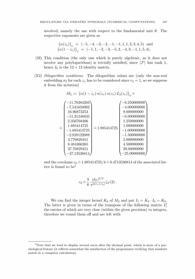
REGULATORS VIA ITERATED INTEGRALS (NUMERICAL COMPUTATIONS) 107
involved, namely the one with respect to the fundamental unit θ. Therespective exponents are given as(
α(zν))ν
= (−5,−4,−3,−2,−1,−1, 1, 1, 2, 3, 4, 5) and(α(1− zν)
)ν
= (−1, 1,−2,−3,−5, 2,−4, 3,−1, 1, 5, 4).
(M) This condition (the only one which is purely algebraic, as it does notinvolve any polylogarithms) is trivially satisfied, since 〈F〉 has rank 1,hence I0 is the 12× 12 identity matrix.
(X2) Dilogarithm conditions. The dilogarithm values are (only the non-realembedding σ2 for each zν has to be considered since r2 = 1, so we suppressit from the notation)
M2 :=(α(1− zν)α(zν)α(zν)L2(zν)
)ν
.=
.=
⎛⎜⎜⎜⎜⎜⎜⎜⎜⎜⎜⎜⎜⎜⎜⎜⎜⎜⎜⎝
−11.78384203−7.54165890216.96873253−11.312488352.3567684061.885414725−1.885414725−2.8281220883.7708294518.48436626537.70829451−47.13536814
⎞⎟⎟⎟⎟⎟⎟⎟⎟⎟⎟⎟⎟⎟⎟⎟⎟⎟⎟⎠
.=1.885414725
⎛⎜⎜⎜⎜⎜⎜⎜⎜⎜⎜⎜⎜⎜⎜⎜⎜⎜⎜⎝
−6.250000000−4.0000000009.000000000−6.0000000001.2500000001.000000000−1.000000000−1.5000000002.0000000004.50000000020.00000000−25.00000000
⎞⎟⎟⎟⎟⎟⎟⎟⎟⎟⎟⎟⎟⎟⎟⎟⎟⎟⎟⎠
and the covolume c2.=1.885414725/4
.=0.4713536814 of the associated lat-
tice is found to be1
c2.=
3
8
|dF |3/2π2(r1+r2)
ζF (2) .
We can find the integer kernel K0 of M2 and put I1 = K0 · I0 = K0.The latter is given in terms of the transpose of the following matrix It1the entries of which are very close (within the given precision) to integers,therefore we round them off and are left with
1Note that we tend to display several zeros after the decimal point, which is more of a psy-chological feature (it reflects somewhat the satisfaction of the programmer verifying that numbersmatch in a computer calculation).

108 HERBERT GANGL
It1 =
⎛⎜⎜⎜⎜⎜⎜⎜⎜⎜⎜⎜⎜⎜⎜⎜⎜⎜⎜⎝
0 0 0 −1 0 0 0 0 0 −1 00 0 1 0 −1 1 1 0 0 0 10 0 0 0 0 1 0 1 0 0 −10 0 −1 1 0 1 0 1 −1 1 10 0 0 −1 0 0 0 0 0 1 01 −1 0 1 0 1 0 −1 0 0 −11 1 0 0 −1 0 −1 0 0 0 00 0 0 0 0 0 1 0 1 1 00 1 −1 0 0 0 0 −1 0 0 00 0 0 0 0 0 1 0 −1 0 00 0 0 0 1 0 0 0 0 0 10 0 0 0 1 0 0 0 0 0 0
⎞⎟⎟⎟⎟⎟⎟⎟⎟⎟⎟⎟⎟⎟⎟⎟⎟⎟⎟⎠
.
Then I1 ·M2.=0.
(Y1) Products of dilogarithms. After those preparations, we can expect con-dition (Y1) to give us a lattice from the matrix with entries products ofdilogarithms
M2,2 :=(α(zν)L2(zν)L2(zν)
)ν
.=
.=
⎛⎜⎜⎜⎜⎜⎜⎜⎜⎜⎜⎜⎜⎜⎜⎜⎜⎜⎜⎝
−1.110871464−0.8886971718−2.666091515−1.777394343−0.2221742929−0.88869717180.22217429290.88869717181.7773943432.6660915150.88869717181.110871464
⎞⎟⎟⎟⎟⎟⎟⎟⎟⎟⎟⎟⎟⎟⎟⎟⎟⎟⎟⎠
.= − 0.2221742929
⎛⎜⎜⎜⎜⎜⎜⎜⎜⎜⎜⎜⎜⎜⎜⎜⎜⎜⎜⎝
5.0000000004.00000000012.000000008.0000000001.0000000004.000000000−1.000000000−4.000000000−8.000000000−12.00000000−4.000000000−5.000000000
⎞⎟⎟⎟⎟⎟⎟⎟⎟⎟⎟⎟⎟⎟⎟⎟⎟⎟⎟⎠
with the covolume c2,2.=0.2221742929 being equal to c22.
Note that I1 ·M2,2 = 0, which shows that both conditions (X2) and(Y1) are needed. Instead, I1 ·M2,2 gives an 11× 1-matrix with commen-surable entries (obvious since M2,2 already does), and one can give aninteger kernel K1 of it and multiply the result by I1. Call the resultingmatrix I2 = K1 · I1; it annihilates both M2 and M2,2. Its transpose isgiven by

REGULATORS VIA ITERATED INTEGRALS (NUMERICAL COMPUTATIONS) 109
It2 =
⎛⎜⎜⎜⎜⎜⎜⎜⎜⎜⎜⎜⎜⎜⎜⎜⎜⎜⎜⎝
0 0 −3 0 0 0 0 0 −3 00 3 0 −3 3 3 0 0 0 30 0 0 0 3 0 3 0 0 −30 −3 3 0 3 0 3 −3 3 30 0 −3 0 0 0 0 0 3 010 −4 −3 12 −25 11 −27 0 0 516 −4 −6 9 −28 8 −24 0 0 80 0 0 0 0 3 0 3 3 03 −3 0 0 0 0 −3 0 0 00 0 0 0 0 3 0 −3 0 00 0 0 3 0 0 0 0 0 30 0 0 3 0 0 0 0 0 0
⎞⎟⎟⎟⎟⎟⎟⎟⎟⎟⎟⎟⎟⎟⎟⎟⎟⎟⎟⎠
.
(X2) Trilogarithmic conditions. The next step is to satisfy condition (X2). Tothis end, we compute the vector of trilogarithms multiplied by the corre-sponding homomorphisms (this time there are r1 + r2 = 2 embeddings σi
of F into C to consider, which is reflected in the notation):
M3 =(α(1− zν)α(zν)L3(σ� zν)
)ν,�
.=
⎛⎜⎜⎜⎜⎜⎜⎜⎜⎜⎜⎜⎜⎜⎜⎜⎜⎜⎜⎝
4.034886241 4.6771634453.081869446 −3.9879051786.013387652 2.4989896986.553788692 0.26499139005.827735082 −3.6517604021.784944975 −1.482786776−4.662188065 2.921408322−2.677417462 2.224180165−2.184596230 −0.088330463343.006693826 1.249494849−15.40934723 19.9395258916.13954496 18.70865378
⎞⎟⎟⎟⎟⎟⎟⎟⎟⎟⎟⎟⎟⎟⎟⎟⎟⎟⎟⎠
.
We find numerically that the rows of I2 ·M3 generate a lattice:

110 HERBERT GANGL
I2 ·M3.=
⎛⎜⎜⎜⎜⎜⎜⎜⎜⎜⎜⎜⎜⎜⎜⎝
−21.09978266 10.549891332.549001106 −6.0827281654.230598524 −5.120441520−9.198456008 45.4691627144.28825961 −16.13384529−2.476557456 1.83930717935.98477232 −7.173874034−12.23789998 0.70969392635.669220069 −5.839752292−21.24466996 19.03673330
⎞⎟⎟⎟⎟⎟⎟⎟⎟⎟⎟⎟⎟⎟⎟⎠
.
The lattice property becomes more apparent if we multiply by the in-verse matrix of the first 2× 2-submatrix of the above and multiply by thecommon denominator 88, the result being:
⎛⎜⎜⎜⎜⎜⎜⎜⎜⎜⎜⎜⎜⎜⎜⎝
88.00000000 0.000000000.00000000 88.00000000
−11.00000000 55.00000000−52.00000000 −748.0000000−198.0000000 −110.00000009.000000000 −11.00000000−174.0000000 −198.000000063.00000000 99.00000000−17.00000000 55.0000000070.00000000 −154.0000000
⎞⎟⎟⎟⎟⎟⎟⎟⎟⎟⎟⎟⎟⎟⎟⎠
.
The determinant c3 of the above 2×2-submatrix is.=101.452557625925282
and it is expressed in terms of Dedekind zeta values via
c3.=
11
9· |dF |
5/2
π3r2ζF (3) .
Again, we can find some matrix K2 which represents the integer kernelof the above, and I3 = K2 · I2 annihilates M2, M2,2 and M3, where itstranspose has the form

REGULATORS VIA ITERATED INTEGRALS (NUMERICAL COMPUTATIONS) 111
It3 =
⎛⎜⎜⎜⎜⎜⎜⎜⎜⎜⎜⎜⎜⎜⎜⎜⎜⎜⎜⎝
2 0 1 3 0 −1 0 −3−1 5 −1 −2 3 0 0 −30 −1 2 0 −2 2 1 0−3 −1 −2 −4 5 2 0 3−2 0 3 1 0 −3 0 −1−7 3 −2 7 −10 3 −2 −7−8 0 4 4 −7 4 −4 −4−2 2 2 0 0 0 4 0−1 −3 1 −1 −1 4 2 −2−2 2 −1 1 0 1 −2 −10 1 −1 −1 2 −1 0 00 0 0 0 −1 0 0 0
⎞⎟⎟⎟⎟⎟⎟⎟⎟⎟⎟⎟⎟⎟⎟⎟⎟⎟⎟⎠
.
(Y2) Products of dilogarithm and trilogarithm. I3 does not annihilate the ex-pressions arising from condition (Y2) which are displayed in the nextequation
M3,2 =(L2(σ1 zν)L3(σ� zν)
)ν,�
.=
⎛⎜⎜⎜⎜⎜⎜⎜⎜⎜⎜⎜⎜⎜⎜⎜⎜⎜⎜⎝
0.3803716968 0.44091964160.3631626273 −0.4699284467−0.9448108025 −0.39263599791.029717475 0.04163488907
−0.5493848770 0.3442541418−0.8413403851 0.69891700600.5493848770 −0.34425414180.8413403851 −0.6989170060−1.029717475 −0.041634889070.9448108025 0.3926359979−0.3631626273 0.4699284467−0.3803716968 −0.4409196416
⎞⎟⎟⎟⎟⎟⎟⎟⎟⎟⎟⎟⎟⎟⎟⎟⎟⎟⎟⎠
(note that for L2 we only use the first embedding) but it gives a latticegenerated by the rows of
I3 ·M3,2.=
⎛⎜⎜⎜⎜⎜⎜⎜⎜⎜⎜⎝
−2.641083126 −0.94583422285.505177483 0.08038099116−1.628466720 −4.001815185−5.607617226 5.92007531913.37917049 −3.573318541−1.699781839 −1.699781839−2.043364556 −4.0776632406.214401668 −3.957091754
⎞⎟⎟⎟⎟⎟⎟⎟⎟⎟⎟⎠,
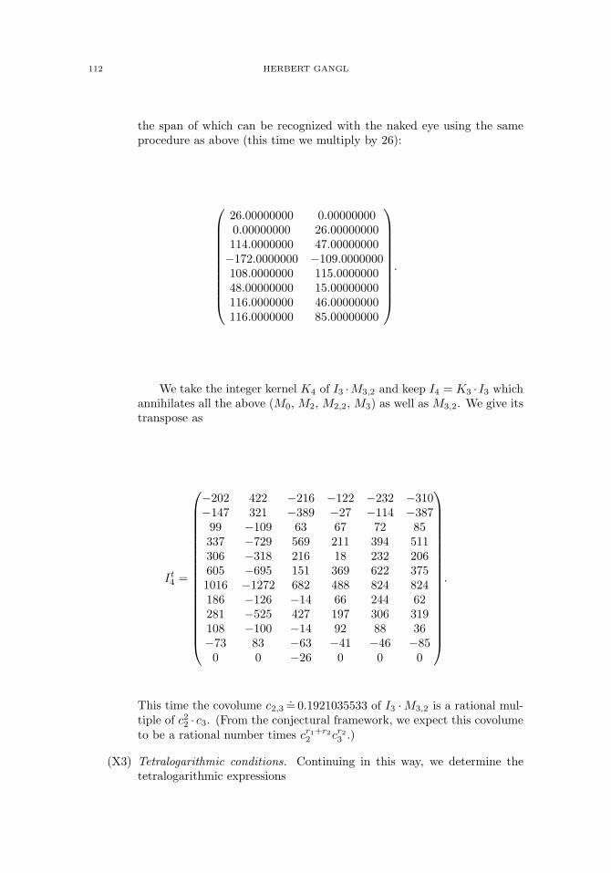
112 HERBERT GANGL
the span of which can be recognized with the naked eye using the sameprocedure as above (this time we multiply by 26):
⎛⎜⎜⎜⎜⎜⎜⎜⎜⎜⎜⎝
26.00000000 0.000000000.00000000 26.00000000114.0000000 47.00000000−172.0000000 −109.0000000108.0000000 115.000000048.00000000 15.00000000116.0000000 46.00000000116.0000000 85.00000000
⎞⎟⎟⎟⎟⎟⎟⎟⎟⎟⎟⎠.
We take the integer kernel K4 of I3 ·M3,2 and keep I4 = K3 · I3 whichannihilates all the above (M0, M2, M2,2, M3) as well as M3,2. We give itstranspose as
It4 =
⎛⎜⎜⎜⎜⎜⎜⎜⎜⎜⎜⎜⎜⎜⎜⎜⎜⎜⎜⎝
−202 422 −216 −122 −232 −310−147 321 −389 −27 −114 −38799 −109 63 67 72 85337 −729 569 211 394 511306 −318 216 18 232 206605 −695 151 369 622 3751016 −1272 682 488 824 824186 −126 −14 66 244 62281 −525 427 197 306 319108 −100 −14 92 88 36−73 83 −63 −41 −46 −850 0 −26 0 0 0
⎞⎟⎟⎟⎟⎟⎟⎟⎟⎟⎟⎟⎟⎟⎟⎟⎟⎟⎟⎠
.
This time the covolume c2,3.=0.1921035533 of I3 ·M3,2 is a rational mul-
tiple of c22 · c3. (From the conjectural framework, we expect this covolumeto be a rational number times cr1+r2
2 cr23 .)
(X3) Tetralogarithmic conditions. Continuing in this way, we determine thetetralogarithmic expressions

REGULATORS VIA ITERATED INTEGRALS (NUMERICAL COMPUTATIONS) 113
M4 =(α(zν)L4(zν)
)ν
.=
⎛⎜⎜⎜⎜⎜⎜⎜⎜⎜⎜⎜⎜⎜⎜⎜⎜⎜⎜⎝
−0.3814538586−0.34563819971.759643788−2.9470035072.9654010971.431744064−2.372320878−2.1476160970.98233450250.87982189421.728190998−1.525815434
⎞⎟⎟⎟⎟⎟⎟⎟⎟⎟⎟⎟⎟⎟⎟⎟⎟⎟⎟⎠
.
Multiplying I4 by M4, we obtain a single column
I4 ·M4.=
⎛⎜⎜⎜⎜⎜⎜⎝
−57.0111864099.01942902−67.01314893−37.00726135−58.01138266−71.01393394
⎞⎟⎟⎟⎟⎟⎟⎠
.=1.0001962525
⎛⎜⎜⎜⎜⎜⎜⎝
−57.0000000099.00000000−67.00000000−37.00000000−58.00000000−71.00000000
⎞⎟⎟⎟⎟⎟⎟⎠.
The covolume c4.=1.0001962525 is found to be
c4.=
135
832· |dF |7/2π4(r1+r2)
· ζF (4) .
The corresponding kernel I5 (simultaneously satisfying all the conditions(X1-3) and (Y1-2)) can be written as the transpose of
It5 =
⎛⎜⎜⎜⎜⎜⎜⎜⎜⎜⎜⎜⎜⎜⎜⎜⎜⎜⎜⎝
−1 −8 5 0 −37 5 14 0 −282 −1 0 0 −4−7 −2 1 1 12−3 0 −9 −16 −920 16 6 −16 −507 2 −7 −16 −3910 8 2 −16 −22−5 −7 8 1 05 2 3 0 −13−1 1 2 0 01 2 −1 0 −1
⎞⎟⎟⎟⎟⎟⎟⎟⎟⎟⎟⎟⎟⎟⎟⎟⎟⎟⎟⎠
.
(D1031) In the last step we compute the values under the “exotic Bloch-Wignerfunction” D10001 as given above, and arrive at

114 HERBERT GANGL
M5 :=(D10001(σ� zν)
)ν,�
.=
⎛⎜⎜⎜⎜⎜⎜⎜⎜⎜⎜⎜⎜⎜⎜⎜⎜⎜⎜⎝
0.3798787865 4.8229871480.3906525699 4.6882192970.8300465454 3.4692597511.231915999 2.6960570381.859803935 1.4583565040.8801812017 3.2432524304.330778718 1.1824778991.346885380 2.4277297734.871430134 1.7139670385.141619571 1.6451788512.153722031 1.3013074235.247265750 1.073768725
⎞⎟⎟⎟⎟⎟⎟⎟⎟⎟⎟⎟⎟⎟⎟⎟⎟⎟⎟⎠
.
The product of I5 and M5 yields the matrix
I5 ·M5.=
⎛⎜⎜⎜⎜⎝
55.64437827 108.533810617.97137546 44.4160916622.97809554 115.5346022−128.5790416 −128.5790416−331.9825665 −424.5390732
⎞⎟⎟⎟⎟⎠
which can be decomposed as
.=
⎛⎜⎜⎜⎜⎝
38.00000000 0.000000000.00000000 38.00000000
−77.00000000 287.0000000−248.0000000 496.0000000−519.0000000 905.0000000
⎞⎟⎟⎟⎟⎠(1.464325743 2.8561529120.4729309331 1.168844517
).
ζF (5): The special value. We can compute the covolume R10001(F ) of I5 ·M5
as
R10001(F ).= 13.71063010
(which is 38 times 0.3608060553, the latter number being the determinantof the 2×2-matrix on the right). Guided by Borel’s theorems, we comparethis number R10001(F ) with the special value
ζF (5).= 1.00041799247384495
and we observe (denoting dF the discriminant of F and r2 the number ofcomplex embeddings which are in our case −23 and 1, respectively):
Experimental Evidence: For the field F of degree 3 over Q and ofdiscriminant dF = −23, the five columns (aj,ν)ν , 1 ≤ j ≤ 5, of It5 give rise
to non-trivial extension classes∑12
ν=1 aj,ν [zν ] in Ext1MTM/F (Q(0),Q(5)),
and moreover their images under (D10001,σ)σ generate a lattice of (full)rank 2 and of covolume R10001(F ) with
|dF |9/2π5r2
· ζF (5) .= 320 ·R10001(F ) .

REGULATORS VIA ITERATED INTEGRALS (NUMERICAL COMPUTATIONS) 115
5.1. Remarks.
(1) The example above is one of the simplest cases that worked, i.e. thatgave a non-zero regulator. Usually the number of zν which are needed toachieve such a non-zero regulator is considerably larger, and more oftenthan not the program does not find sufficiently many of them.
(2) The procedure of taking the kernel rationally is numerically highly unsta-ble, and since we want to be able to recognize a lattice, it is crucial that wefind generators of the kernels which form a Z-basis for the lattice (or whichare at least not far away from this property, i.e. the denominator shouldbe bounded). The problem is that, for the matrix entries we encounter, itmay take very long to find such a Z-basis already for, say, a lattice givenby a matrix of size 300×600. The number of conditions grows very fastwith the order of S and it is typically impractical to include more than 3or 4 primes into S.
(3) One can view the above weight 5 function as a multiple polylogarithmas introduced by Goncharov (see e.g. [8]), but specialized to one variableonly (then also called “generalized polylogarithm” in the literature), andthose multiple polylogarithms in turn have appeared early as “hyperloga-rithms”, in particular in work of Lappo-Danilevsky [11]. In this setting thefunction above is denoted Li4,1(1, z), and it might be tempting to think ofthe resulting special value not as a Dedekind zeta value ζF (5) but as a kindof “multiple Dedekind zeta value” ζF (4, 1) (for some candidates see Wojt-kowiak’s original article [13]) which then would seem, modulo the prod-uct ζF (2)ζF (3), to be a rational multiple of the former, similar to what isknown to be true for F = Q where one has ζ(4, 1) = 5ζ(5)−ζ(2)ζ(3). Alas,we were unable to give a sensible evaluation of such a multiple Dedekindzeta value which might have corroborated such a statement.
6. Further results
6.1. Totally real fields. The simplest cases to consider seem to be the oneswhich are totally real, as the conditions involving dilogarithms and tetralogarithmsall are trivially satisfied, since the function L2n(z) vanishes on the real line. Nev-ertheless, they turn out to be hard, due to complexity reasons (the integer kernelsinvolved tend to have large coefficients).
6.1.1. The case F = Q. In the case of the rational numbers we also find anon-trivial result; using the set S = 〈2, 3, 5〉 , we find 98 exceptional S-units, anda similar calculation as above, but where we only need to satisfy conditions (M),followed by (X2) which produces a (numerical) lattice of covolume ζ(3)/96, gives usa lattice generated by the image under D10001 of 50 linear combinations in Z[F ], ofcovolume 1
480ζ(5) (and we get the same lattice if we add the prime 7 to S, yielding178 exceptional S–units and 87 generators of the lattice).
6.2. Other number fields. We have obtained similar results for numberfields of degree ≤ 6, typically we were lucky to find a full regulator lattice forsome small discriminants. We list signatures and corresponding discriminants forwhich we have obtained a (conjectural) lattice of full rank r1 + r2:

116 HERBERT GANGL
signature discriminants(2, 0) 5, 8, 13(0, 1) −3, −7, −8, −15, −20(1, 1) −31, −44, −59, −76, −83, −104, −108, −116, −139, −152(3, 0) 49, 148, 229(2, 1) −275, −283, −331, −400, −448(4, 0) 725, 1125(0, 3) −9747 .
Moreover, if we divide the covolume of the (conjectural) lattice of D10001–values
by |dF |9/2π−5r2ζF (5), the result in each case is numerically close to a rationalnumber of small height.
For many other number fields, the height (or complexity) of the rational num-bers in the inductive steps explodes quickly and gets out of control.
Acknowledgements. We are very grateful to Zdzis�law Wojtkowiak for notonly drawing our attention to the questions surrounding his formalism, but also forcommunicating the appropriate tools in a down-to-earth language which made itpossible to have it implemented. We express our gratitude to the University of Nicefor supporting several research visits, as well as to the Institute for ExperimentalMathematics in Essen and the Max–Planck–Institute in Bonn and the Isaac NewtonInstitute in Cambridge for providing an inspiring environment, and to the DFGfor long-term financial support. Finally we want to thank Hiroaki Nakamura forseveral clarifications and in particular the referee for many very helpful remarkswhich improved the exposition considerably.
References
[1] Beilinson, A. and Deligne, P.; Interpretation motivique de la conjecture de Zagier reliantpolylogarithmes et regulateurs, Motives (Seattle, WA, 1991), 97–121, Proc. Sympos. Pure
Math., 55, Part 2, Amer. Math. Soc., Providence, RI, 1994.[2] Beilinson, A. and Deligne, P.; Motivic polylogarithms and Zagier’s conjecture, Preprint
1992.[3] Bloch, S.; Higher regulators, algebraic K-theory, and zeta functions of elliptic curves, CRM
Monograph Series, 11. American Mathematical Society, Providence, RI, 2000 (known also as“Irvine Lecture Notes”, 1978).
[4] Borel, A.; Cohomologie de SLn et valeurs de fonctions zeta aux points entiers, Ann. ScuolaNorm. Sup. Pisa Cl. Sci. (4) 4 (1977), no. 4, 613–636.
[5] Brown, F.; Polylogarithmes multiples uniformes en une variable, C. R. Math. Acad. Sci.Paris 338 (2004), no. 7, 527–532.
[6] Cohen, H., Lewin, L. and Zagier, D.; A sixteenth order polylogarithmic ladder, Experi-ment. Math. vol. 1, 1992, 25–34.
[7] Deligne, P. and Goncharov, A.B.; Groupes fondamentaux motiviques de Tate mixte,
Ann. Sci. Ecole Norm. Sup. (4) 38 (2005), no. 1, 1–56.[8] Goncharov, A.B.; Multiple polylogarithms, cyclotomy and modular complexes, Math. Res.
Lett. 5 (1998), no. 4, 497–516.[9] The PARI–Group; PARI/GP, versions 2.1-2.4, Bordeaux, http://pari.math.
u-bordeaux.fr/.[10] de Jeu, R.; Zagier’s conjecture and wedge complexes in algebraic K-theory, Compositio
Math. 96 (1995), no. 2, 197–247.[11] Lappo-Danilevsky, J. A.; Memoires sur la theorie des systemes des equations
differentielles lineaires, Chelsea Publishing Co., New York, N. Y., 1953.[12] Lewin, L.; Polylogarithms and associated functions, North-Holland, New York-Amsterdam,
1981.
REGULATORS VIA ITERATED INTEGRALS (NUMERICAL COMPUTATIONS) 117
[13] Wojtkowiak, Z.; Mixed Hodge Structures and Iterated Integrals I, in “Motives, polyloga-rithms and Hodge theory, Part I” (Irvine, CA, 1998), 121–208, Int. Press Lect. Ser., 3, I, Int.Press, Somerville, MA, 2002.
[14] Wojtkowiak, Z.; Monodromy of iterated integrals and non-abelian unipotent periods, in“Geometric Galois actions”, 2, 219–289, London Math. Soc. Lecture Note Ser., 243, Cam-bridge Univ. Press, Cambridge, 1997.
[15] Zagier, D.; Polylogarithms, Dedekind zeta functions and the algebraic K-theory of fields,
Proc. Texel Conf. on Arithm. Alg. Geometry 1989, Birkhauser, Boston (1991) 391–430.
Department of Mathematical Sciences, South Road, University of Durham, DH1
3LE, United Kingdom
E-mail address: [email protected]


Clay Mathematics ProceedingsVolume 9, 2010
Zero-cycles on algebraic tori
Alexander S. Merkurjev
1. The map ϕT
Let T be an algebraic torus over a field F and X a smooth compactificationof T , i.e., a geometrically irreducible smooth complete variety containing T as anopen set. The Chow group CH0(X) of classes of zero dimensional cycles on X doesnot depend (up to canonical isomorphism) on the choice of X (cf. [7, 16.1.11], [4,Prop. 6.3], [8]).
Recall that two F -points t, t′ ∈ T (F ) are called R-equivalent if there is rationalmorphism f : A1 ��� T defined at 0 and 1 satisfying f(0) = t and f(1) = t′ (cf. [2,§4]). We write T (F )/R for the group of R-equivalence classes in T (F ).
For an F -point t ∈ T (F ) let [t] denote its class in CH0(X). Consider the mapfrom T (F ) to CH0(X) taking a point t to the class [t] − [1]. This map does notdepend on the choice of X (up to canonical isomorphism) and it factors throughR-equivalence. Indeed, a map f as above extends to a morphism g : P1 → X and[t] = g∗([0]) = g∗([1]) = [t′], where g∗ : CH0(P
1) → CH0(X) is the push-forwardhomomorphism (cf. [7, 1.4]).
We denote the resulting map by
ϕT : T (F )/R → CH0(X).
Note that there is a homomorphism ψT : A0(X) → T (F )/R such that ψT ◦ϕT
is the identity (cf. [2, Prop. 12]). It follows that the map ϕT is injective.One can ask whether ϕT is a homomorphism. It is known that ϕT is a homo-
morphism for all tori T of dimension at most 3 (cf. [10]). In this note we shall givean example of a torus T such that ϕT is not a homomorphism although it has leftinverse map ψT that is a homomorphism. It follows that ϕT is not surjective.
The map ϕT is a homomorphism if and only if for any two points t1 and t2 inT (F ) one has
(1) [t1t2]− [t1]− [t2] + [1] = 0
in CH0(X).
2010 Mathematics Subject Classification. 14C25.Key words and phrases. Algebraic cycles, Algebraic tori.The work has been supported by the NSF grant DMS #0652316.
c© 2010 Alexander S. Merkurjev
119

120 A. MERKURJEV
Let T ′ be another torus with a compactification X ′. Then X × X ′ is a com-pactification of T × T ′. Let t ∈ T (F ) and t′ ∈ T ′(F ). The condition (1) for theelements t1 = (t, 1) and t2 = (1, t′) of (T × T ′)(F ) amounts to
(2) ([t]− [1])× ([t′]− [1]) = 0
in CH0(X ×X ′), where × denotes the external product for Chow groups (cf. [7,1.10]). In the next section we shall give examples of tori T and T ′ such thatthe condition (2) fails for some t and t′. It would follows that ϕT×T ′ is not ahomomorphism.
2. The tori R1L/F (Gm)
Let F be a field with charF �= 2. For an element a ∈ F×, let Fa denote thequadratic (etale) F -algebra F [t]/(t2 − a).
Let a, b ∈ F×. Consider the biquadratic F -algebra L = Fa ⊗ Fb and let G bethe Galois group Gal(L/F ). Write σ ∈ G for the generator of Gal(L/Fa) and τ ∈ Gfor the generator of Gal(L/Fb).
Let T be the torus R1L/F (Gm) of norm 1 elements of the extension L/F . For
a field extension K/F , a point t of T (K) is an element t ∈ (K ⊗ L)× satisfyingN(K⊗L)/K(t) := t · σ(t) · τ (t) · στ (t) = 1, where N(K⊗L)/K : (K ⊗L)× → K× is thenorm homomorphism. The element N(K⊗L)/(K⊗Fa) = t · σ(t) in K ⊗ Fa has norm1 in K. By Hilbert Theorem 90, applied to the quadratic extension (K ⊗ Fa)/K,there is an element z ∈ (K⊗Fa)
× with t ·σ(t) = z ·τ (z)−1. Note that z is unique upto a multiple from K×. Hence the norm N(K⊗Fa)/K(z) = z · τ (z) is unique up to a
multiple from K×2. It follows that the class qK(t) quaternion algebra(z · τ (z), b
)K
in the Brauer group Br(K) is well defined. Thus, we get a group homomorphism
qK : T (K) → Br(K), t �→ qK(t).
The collection of the homomorphisms qK over all field extensions K of F form amorphism q of functors T and Br from the category of all field extensions of F tothe category of groups. In other words, q is an invariant of the algebraic torus Twith values in the Brauer group (cf. [9]).
Remark 2.1. It is shown in [11, p. 427] that qF induces an isomorphism betweenT (F )/R and the subgroup of Br(F ) consisting of classes of algebras that are splitover all three quadratic subalgebras of L.
Example 2.2. Assume that F contains a square root i of −1. Then we can view ias an element of T (F ). We have i ·σ(i) = −1 = z ·τ (z)−1 with z =
√a in Fa. Hence
qF (i) is the class of the quaternion algebra(z · τ (z), b
)F
(−a, b
)F
(a, b
)F.
Let F (T ) be the function field of T over F and let v be a discrete valuation onF (T ) over F . The residue field F (v) is a field extension of F . By [5, §5], there isthe residue homomorphism
∂v : Br(L(T )/F (T )
)→ G∗,
where G∗ is the character group of G. An element α in Br(L(T )/F (T )
)is called
unramified with respect to v if ∂v(α) = 0 and (totally) unramified if α is unramifiedwith respect to every discrete valuation of F (T ) over F .
Proposition 2.3. For any t ∈ T(F (T )
), the element qF (T )(t) in Br
(L(T )/F (T )
)is unramified.
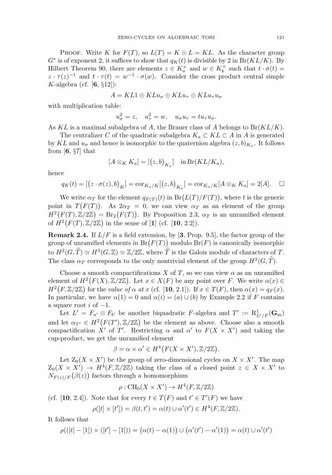
ZERO-CYCLES ON ALGEBRAIC TORI 121
Proof. Write K for F (T ), so L(T ) = K ⊗ L = KL. As the character groupG∗ is of exponent 2, it suffices to show that qK(t) is divisible by 2 in Br(KL/K). ByHilbert Theorem 90, there are elements z ∈ K×
a and w ∈ K×b such that t · σ(t) =
z · τ (z)−1 and t · τ (t) = w−1 · σ(w). Consider the cross product central simpleK-algebra (cf. [6, §12]):
A = KL1⊕KLuσ ⊕KLuτ ⊕KLuτuσ
with multiplication table:
u2σ = z, u2
τ = w, uσuτ = tuτuσ.
As KL is a maximal subalgebra of A, the Brauer class of A belongs to Br(KL/K).The centralizer C of the quadratic subalgebra Ka ⊂ KL ⊂ A in A is generated
by KL and uσ and hence is isomorphic to the quaternion algebra (z, b)Ka. It follows
from [6, §7] that[A⊗K Ka] = [
(z, b
)Ka
] inBr(KL/Ka),
hence
qK(t) = [(z · σ(z), b
)K] = corKa/K [
(z, b
)Ka
] = corKa/K [A⊗K Ka] = 2[A]. �
We write αT for the element qF (T )(t) in Br(L(T )/F (T )
), where t is the generic
point in T(F (T )
). As 2αT = 0, we can view αT as an element of the group
H2(F (T ),Z/2Z
)= Br2
(F (T )
). By Proposition 2.3, αT is an unramified element
of H2(F (T ),Z/2Z
)in the sense of [1] (cf. [10, 2.2]).
Remark 2.4. If L/F is a field extension, by [3, Prop. 9.5], the factor group of thegroup of unramified elements in Br
(F (T )
)modulo Br(F ) is canonically isomorphic
to H2(G, T ) H3(G,Z) Z/2Z, where T is the Galois module of characters of T .
The class αT corresponds to the only nontrivial element of the group H2(G, T ).
Choose a smooth compactifications X of T , so we can view α as an unramifiedelement of H2
(F (X),Z/2Z
). Let x ∈ X(F ) be any point over F . We write α(x) ∈
H2(F,Z/2Z
)for the value of α at x (cf. [10, 2.1]). If x ∈ T (F ), then α(x) = qF (x).
In particular, we have α(1) = 0 and α(i) = (a) ∪ (b) by Example 2.2 if F containsa square root i of −1.
Let L′ = Fa′ ⊗ Fb′ be another biquadratic F -algebra and T ′ := R1L′/F (Gm)
and let αT ′ ∈ H2(F (T ′),Z/2Z
)be the element as above. Choose also a smooth
compactification X ′ of T ′. Restricting α and α′ to F (X × X ′) and taking thecup-product, we get the unramified element
β = α× α′ ∈ H4(F (X ×X ′),Z/2Z
).
Let Z0(X ×X ′) be the group of zero-dimensional cycles on X ×X ′. The mapZ0(X × X ′) → H4(F,Z/2Z) taking the class of a closed point z ∈ X × X ′ toNF (z)/F
(β(z)
)factors through a homomorphism
ρ : CH0(X ×X ′) → H4(F,Z/2Z)
(cf. [10, 2.4]). Note that for every t ∈ T (F ) and t′ ∈ T ′(F ) we have
ρ([t]× [t′]) = β(t, t′) = α(t) ∪ α′(t′) ∈ H4(F,Z/2Z).
It follows that
ρ(([t]− [1])× ([t′]− [1])) =(α(t)− α(1)
)∪(α′(t′)− α′(1)
)= α(t) ∪ α′(t′)

122 A. MERKURJEV
in H4(F,Z/2Z).Assume that F contains a square root i of −1, so i ∈ T (F ). We then have
ρ(([i]− [1])× ([i]− [1])
)= (a) ∪ (b) ∪ (a′) ∪ (b′) ∈ H4(F,Z/2Z).
One can easily find a field F and elements a, b, a′, b′ with (a) ∪ (b) ∪ (a′) ∪ (b′) �= 0in H4(F,Z/2Z). For example, one can take F = k(a, b, a′, b′), where a, b, a′, b′ arevariables over a field k. This contradicts (2). Hence ϕT×T ′ is not a homomorphism.
References
[1] J.-L. Colliot-Thelene, Birational invariants, purity and the Gersten conjecture, K-theory andalgebraic geometry: connections with quadratic forms and division algebras (Santa Barbara,CA, 1992), Amer. Math. Soc., Providence, RI, 1995, pp. 1–64.
[2] J.-L. Colliot-Thelene and J.-J. Sansuc, La R-equivalence sur les tores, Ann. Sci. Ecole Norm.Sup. (4) 10 (1977), no. 2, 175–229.
[3] J.-L. Colliot-Thelene and J.-J. Sansuc, Principal homogeneous spaces under flasque tori: ap-plications, J. Algebra 106 (1987), no. 1, 148–205.
[4] J.-L. Colliot-Thelene and D. Coray, L’equivalence rationnelle sur les points fermes des surfacesrationnelles fibrees en coniques, Compositio Math. 39 (1979), no. 3, 301–332.
[5] J.-L. Colliot-Thelene and J.-J. Sansuc, The rationality problem for fields of invariants underlinear algebraic groups (with special regards to the Brauer group), Algebraic groups and ho-mogeneous spaces, Tata Inst. Fund. Res. Stud. Math., Tata Inst. Fund. Res., Mumbai, 2007,pp. 113–186.
[6] P. K. Draxl, Skew fields, London Mathematical Society Lecture Note Series, vol. 81, CambridgeUniversity Press, Cambridge, 1983.
[7] W. Fulton, Intersection theory, Springer-Verlag, Berlin, 1984.[8] A. Merkurjev, Rational correspondences,
http://www.math.ucla.edu/ merkurev/publicat.htm (2004).[9] A. Merkurjev, Invariants of algebraic groups, J. Reine Angew. Math. 508 (1999), 127–156.[10] A. Merkurjev, Unramified elements in cycle modules, J. London Math. Soc. 78 (2008), no. 1,
51–64.[11] J.-P. Tignol, Produits croises abeliens, J. Algebra 70 (1981), no. 2, 420–436.
Department of Mathematics, University of California, Los Angeles, CA 90095-1555,
USA
E-mail address: [email protected]

Clay Mathematics ProceedingsVolume 9, 2010
Chow-Kunneth projectors and �-adic cohomology
Andrea Miller
1. Introduction
This article deals with motivic decompositions of Chow motives of universal familiesover certain Shimura varieties of PEL-type. “PEL-type” means that the universalfamily is given by a family of abelian varieties with polarization, endomorphism andlevel structure. Absolute Chow-Kunneth decompositions of such families (meaningChow-Kunneth decompositions of the total space of such a family) were proven toexist by the author in [25] in the case of families over compact unitary Shimuravarieties of a certain type. These results were the content of the author’s talk atthe conference. They are the motivation and starting point for the present articleand we will give a very short account on them in Section 3. For more details see[25] and [26] directly.
The main objective of the present article is to relate our Chow-Kunneth projec-tors obtained in [25] to certain projectors in the ring of endomorphisms of �-adiccohomology. As base variety we take the compact unitary Shimura varieties usedin [16] and studied in [20] and [9]. We then relate the �-adic realizations of Chowmotives, cut out by suitable projectors in the Chow ring, with homological motiveswhich are cut out by projectors in the �-adic cohomology of these Shimura varieties.The homological projectors we use are the Kunneth projectors used in [16]. TheChow-Kunneth projectors we relate them to are the ones constructed by the authorin [25]. For the fibres of the universal abelian scheme over the Shimura variety thisis done in Section 5.
As simple as the definition of a Chow motive is, we know very little about them.Thus working out problems usually means working with a specific realization of aChow motive. Yet this is often not fully satisfying for obtaining a purely algebraicgeometric understanding of how motives decompose. For example in the cohomol-ogy of Shimura varieties Hecke correspondences are the essential tool to decomposethese Grothendieck motives. Yet, if and how these “Hecke decompositions” lift todecompositions of corresponding Chow motives is widely unknown.
c© 2010 Andrea Miller
123
124 ANDREA MILLER
The contents of this article are as follows. In section 2 we recall the terminology ofChow motives and explain Murre’s conjecture. In section 3 we give a short intro-duction to our work [25]. In section 4 we first recall the definition of Fourier-Mukaitransform. Fourier-Mukai transforms were the essential tool in constructing mo-tivic decompositions of abelian schemes (see [10]) and we then explain the resultswe need. In an upcoming paper we treat Fourier-Mukai transforms for compactifi-cations of 1-motives. This, we hope, will be useful to treat Murre’s Conjecture ina more general context of Shimura varieties which are neither compact nor relatedto Gl2 (as are modular curves or Hilbert modular varieties, which were treated in[15], [12]).Finally in Section 5 we relate our Chow-Kunneth projectors to projectors of �-adic cohomology for universal families over the above mentioned compact unitaryShimura varieties.
It is a pleasure to thank the organizers of the conference for organizing such aninteresting conference. I especially want to thank Roy Joshua for his patience.I thank the referee for useful comments. This work was partly supported by aresearch grant of the “Deutsche Forschungsgemeinschaft”.
2. Standard Conjecture “C” and Murre’s Conjecture
2.1. In this paragraph, we recall the basic theory of Chow motives, especiallyas related to Murre’s Conjecture. Further details may be found in [27].For a smooth projective variety Y over a field k let CHj(Y ) denote the Chow groupof algebraic cycles of codimension j on Y modulo rational equivalence, and letCHj(Y )Q := CHj(Y )⊗Q. For a cycle Z on Y we write [Z] for its class in CHj(Y ).We will be working with relative Chow motives as well, so let us fix a smoothconnected, quasi-projective base scheme S → Spec k. If S = Spec k, we typicallywrite X ×k Y for X ×Spec k Y . Let Y, Y ′ be smooth projective varieties over S, i.e.,all fibers are smooth. For our purposes we may assume that Y is irreducible andof relative dimension g over S. The group of relative correspondences from Y to Y ′
of degree r is defined as
Corrr(Y ×S Y ′) := CHr+g(Y ×S Y ′)Q.
Every S-morphism Y ′ → Y defines an element in Corr0(Y ×S Y ′) via the class ofthe transpose of its graph. In particular one has the class [ΔY/S ] ∈ Corr0(Y ×S Y )of the relative diagonal. The self correspondences of degree 0 form a ring, see [27,p. 127]. Furthermore there is a ring homomorphism
(∗) CH∗(Y × Y ) −→ End(CH∗(Y ))
([11], Corollary 16.1.2). This yields an action of correspondences on Chow groups.Using the relative correspondences one proceeds as usual to define the categoryCHM(S) of (pure) Chow motives over S. The objects of this pseudoabelian Q-linear tensor category are triples (Y, p, n) where Y is as above, p is a projector, i.e.an idempotent element in Corr0(Y ×S Y ), and n ∈ Z. The morphisms are
HomMS((Y, p, n), (Y ′, p′, n′)) := p′ ◦ Corrn
′−n(Y ×S Y ′) ◦ p.
When n = 0 we write (Y, p) instead of (Y, p, 0), and h(Y ) := (Y, [ΔY ]).

CHOW-KUNNETH PROJECTORS AND �-ADIC COHOMOLOGY 125
2.2. Murre’s conjectures. Let k be a field. Fix a Weil cohomology theoryH∗ and a smooth projective variety Y over k with dimY = d. Then by the Kunnethformula we have
H2d(Y × Y )(d) = ⊕2dn=0H
n(Y )⊗H2d−n(Y )(d).
Since Y is projective, by Poincare duality, we have
H2d−n(Y )(d) = Hn(Y )∨.
We then get
H2d(Y × Y )(d) = ⊕2dn=0H
n(Y )⊗Hn(Y )∨
= ⊕2dn=0 Hom(Hn(Y ), Hn(Y )).
We can thus identify H2d(Y ×Y )(d) with the vector space of graded k-linear mapsf : H∗(Y ) −→ H∗(Y ). In particular we can write
idH∗(Y ) =
2d∑n=0
πnY where πn
Y ∈ Hn(Y )⊗Hn(Y )∨.
The projectorπnY : H∗(Y ) −→ H∗(Y )
is called the n-th Kunneth projector.Denote the cycle class map by
cl : CH∗(Y ) −→ H2∗(Y )
for a chosen Weil cohomology H∗(·). Recall that a class in H∗(Y ) is called algebraicif it lies in the image of the cycle class map cl.
Conjecture 2.1 (Grothendieck). The Kunneth projectors
πnY : H∗(Y ) −→ H∗(Y ), n = 0 . . . 2d
are algebraic.
As the diagonal [ΔY/k] ∈ CHd(Y × Y ) is mapped to idH∗(Y ) by the cycle classmap we can ask further if the πn
Y , (n = 0, . . . 2d) lift to orthogonal projectors
π0, . . . , π2d ∈ CHd(Y × Y ).
Definition 2.2. For a smooth projective variety Y/k of dimension d a Chow-Kunneth-decomposition of Y consists of a collection of pairwise orthogonal projec-tors π0, . . . , π2d in Corr0(Y × Y ) satisfying
(1) π0 + . . .+ π2d = [ΔY ] and(2) for some Weil cohomology theory H∗ one has πi(H
∗(Y )) = Hi(Y ).
If one has a Chow-Kunneth decomposition for Y one writes hi(Y ) = (Y, πi). Asimilar notion of a relative Chow-Kunneth-decomposition over S can be defined ina straightforward manner, see [27].
The existence of such a decomposition for every smooth projective variety is partof the following conjecture of Murre:
126 ANDREA MILLER
Conjecture 2.3 (Murre). Let Y be a smooth projective variety of dimension dover some field k.
(1) There exists a Chow-Kunneth decomposition for Y .(2) For all i < j and i > 2j the action of πi on CHj(Y )Q ( see (∗) in section
2.1 ) is trivial, i.e. πi · CHj(Y )Q = 0.(3) The induced j step filtration on
F νCHj(Y )Q := Kerπ2j ∩ · · · ∩Kerπ2j−ν+1
is independent of the choice of the Chow–Kunneth projectors.(4) The first step of this filtration should give exactly the subgroup of homo-
logical trivial cycles in CHj(Y )Q.
Remark 2.4. Jannsen showed in [19] that this conjecture is equivalent to theBloch-Beilinson conjecture.
Convention 2.5. We will follow the general convention of calling part (1) of theabove conjecture of Murre ” Murre’s Conjecture ”. It can be seen as a strengtheningof Grothendieck’s conjecture ”C” and this is the part of the above conjecture wewill be concerned with in this article.
There are not many cases for which Murre’s conjecture (e.g. as by the aboveconvention the existence of a Chow-Kunneth decomposition) has been proved. It isknown to be true for curves and surfaces [27]. See also the above mentioned work ofJannsen [19] over finite fields (where a lot more is proved). Furthermore for abelianschemes over a smooth projective base, Deninger and Murre have constructed arelative Chow-Kunneth decomposition in [10], generalizing work of Shermenev [29]and Beauville ([3], [4]). Apart from the work already mentioned and the workon families over Shimura varieties, which will be the content of the next section,special cases have been treated among others by Akhtar-Joshua [1], del Angel-Muller-Stach [2], Brosnan [5], Iyer ([17],[18]). We will now proceed to the resultswhich are known for universal families over Shimura varieties.
3. Murre’s Conjecture and mixed Shimura varieties
As for mixed Shimura varieties, the basic method of approach was established inthe cases of families over modular curves and Hilbert modular varieties by Gor-don, Hanamura and Murre, see [12], [13], [14], [15]. Certain families over Picardmodular surfaces were incompletely treated in [24]. A complete Chow-Kunnethdecomposition for some mixed Kottwitz Shimura varieties was constructed by theauthor in [25]. In [25] the approach of Gordon, Hanamura and Murre was modifiedto cover more general Shimura varieties. There we also proved that necessary con-ditions assumed in this approach were fulfilled in all the cases mentioned above. So,at the present moment, the known cases involving Shimura varieties are restrictedfirst to some Shimura varieties arising from Gl2 (Gordon, Hanamura, Murre) andsecondly to the author’s work on compact Shimura surfaces arising from certainunitary groups associated to division algebras [25] . We will now indicate how theresults of [25] were obtained. Proofs for all the results we present here can be foundin [25].
Consider the following situation. For simplicity let our ground field be C. Let Xbe a compact Shimura variety of Kottwitz type (i.e. smooth projective over SpecCof a certain unitary type, see [25]) and let A/X in

CHOW-KUNNETH PROJECTORS AND �-ADIC COHOMOLOGY 127
A
π
��
p
��X
��SpecC
be an abelian scheme over X. Let At denote the fibre of A over a point t ∈X. Then the first Betti homology group of At carries a Hodge structure of type(−1, 0), (0,−1) and we denote its Hodge group by Hod(At).In [25] we prove the following theorem. A weaker version of this theorem goes backto work of Gordon, Hanamura and Murre in [15]. See (ii) of the Remarks 3.2 below.
Theorem 3.1. Let p : A → X as above be surjective, smooth and projective satis-fying the following conditions:
(1) The scheme A/X has a relative Chow-Kunneth decomposition.(2) X has a Chow-Kunneth decomposition over C.(3) If t is a point of X the natural map.
CHr(A) → H2rB (At(C),Q)Hod(At)
is surjective for 0 ≤ r ≤ d = dimA− dimX.(4) For i odd, Hi
B(At(C),Q)Hod(At) = 0 (redundant condition).(5) Let ρ be an irreducible, non-constant representation of Hod(At) and V the
corresponding local system on X.Then the cohomology Hq(X,V) vanishes if q = dimX.
Under these assumptions A has a Chow-Kunneth decomposition over C.
�The proof of this theorem is rather technical and we will not comment on it. Theinterested reader should consult our paper [25] directly. In [25] we then proceedto verify assumptions (1) - (5) of Theorem 3.1 in the case of a compact unitaryShimura surface S of Kottwitz type. By the conclusion of Theorem 3.1, this thenyields Chow-Kunneth decompositions for the corresponding total space.
Remarks 3.2. (i) The fundamental strategy of the proof goes back to [15].The main new insight for the proof in our case is the fact, that we need toweaken the assumptions on monodromy of [15] since these assumptionsare false in more general cases. Generally the hypotheses of Theorem 1.3.of [15] are too strong even in the compact case, so there is very little hopeof being able to use it for non-compact Shimura varieties beyond the onesstudied in [15]. See [24] for a non-trivial low-dimensional case where theprerequisites of Theorem 1.3. of [15] fail.
(ii) To remedy the problems described in (ii), the main observation is tosystematically work with Mumford-Tate groups instead of fundamentalgroups as was done in all of the previous work on other cases given byShimura varieties ([12], [15]).

128 ANDREA MILLER
4. Fourier-Mukai transforms for Abelian schemes
Let us shortly recall the definition of Fourier-Mukai transform. For a general refer-ence on Fourier-Mukai transforms we refer to [6].
Let X −→ S, Y −→ S be smooth projective schemes X,Y over a smooth quasi-projective scheme S. Denote by p (resp. q) the projectors from X ×S Y to X/S(resp. Y/S).Let cohomology be singular cohomology with coefficients inQ. Recall thatH∗(X,Q)comes equipped with a ring structure. For f : X −→ Y denote by f∗ and f∗ theinduced morphisms on H∗. Fourier-Mukai transformation is defined as follows:
Definition 4.1. LetX,Y, p, q be as above. Then for any a ∈ H∗(X×Y ) (“kernel”),define the cohomological Fourier-Mukai transform associated to a to be
ΦHa : H∗(X,Q) −→ H∗(Y,Q)
b �→ q∗(a · p∗(b)).A similar definition holds for Fourier-Mukai transforms between Chow groups, thekernel then being an element a ∈ CH∗(X × Y ).
We will now specialize the situation to our purpose, namely to abelian schemesA/S. Fourier-Mukai transforms between abelian varieties and their duals were atthe origins of Mukai’s work on Fourier-Mukai transforms. He used them to showthat the bounded derived category of an abelian variety is equivalent to the boundedderived category of its dual.They were further used by Beauville ([3],[4]), generalizing work of Shermenev[29], to give a motivic decomposition of abelian varieties. This was generalizedby Deninger and Murre [10] to give a motivic decomposition of abelian schemesover smooth quasi-projective bases.We will now briefly recall the results from Deninger and Murre (see [10]), whichwe will need later.Denote by A/S an abelian scheme, by A/S its dual, by n : A −→ A multiplication
by n ∈ Z on A and by n = idA × n : A×S A −→ A×S A.Fourier-Mukai transform from CH∗(A) to CH∗(A) are constructed by using a
Poincare line bundle P on A× A as kernel. Pick such a P and rigidify it along thezero section. It is then known [10] that
n∗(x) = nx in CH1(A×S A).
Following Beauville ([3], [4]), Deninger and Murre [10] defined the following eigenspacesof CHi(A,Q) with respect to n∗:
CHis(A,Q) := {y ∈ CHi(A,Q) | n∗y = n2i−sy for all n ∈ Z}.
CHOW-KUNNETH PROJECTORS AND �-ADIC COHOMOLOGY 129
Generalizing the above mentioned results of Beauville, Deninger and Murre [10]prove (their Theorem 2.19)
Theorem 4.2. Let A/S an abelian scheme of fibre dimension g and let d = dimS.Then for all i we have
CHi(A,Q) =
l⊕s=k
CHis(A,Q)
with k = Max(i− g, 2i− 2g) and l = Min(2i, i+ d).
�
For the abelian scheme A ×S A over A/S (via projection on the first factor) onederives
Corollary 4.3. Let A/S an abelian scheme of fibre dimension g. Then for all iwe have
CHi(A×S A,Q) =
l⊕s=k
CHis(A×S A,Q)
with k = Max(i− g, 2i− 2g) and l = Min(2i, i+ g).
Proof. Apply theorem 4.2 to the abelian scheme A ×S A over A/S. Therelative dimension of A×S A over A/S is again g. �
If we now apply this corollary to the degree i = g component of the Chow groupwe get the following “eigenspace” decomposition of CHg(A×S A):
CHg(A×S A) =
2g⊕s=0
CHgs (A×S A,Q).
As explained in section 2, we are particularly interested in one very specific cyclein CHg(A×S A,Q), namely the diagonal ΔA/S , which will lead to Chow-Kunnethdecompositions.
4.1. Projectors for Abelian Varieties. Let S be a fixed base scheme. Werecall the Chow-Kunneth decomposition of an abelian scheme A of fibre dimensiong over S (see [10]). For n ∈ N let [n] denote the cycle class induced from multipli-cation by n on A/S. (Yet, we will stick with [ΔA/S ] as notation for the Chow classof ΔA/S .)Firstly we have a functorial decomposition of the relative diagonal ΔA/S .
Theorem 4.4. There is a unique decomposition
[ΔA/S ] =
2g∑s=0
πi in CHg(A×S A)Q
such that (idA × [n])∗πi = niπi for all n ∈ Z. Moreover the πi are mutually or-thogonal idempotents, and [tΓ[n]] ◦ πi = niπi = πi ◦ [tΓ[n]], where [n] denotes themultiplication by n on A.
Proof. This is Theorem 3.1 of [10].�
As a corollary they obtain
130 ANDREA MILLER
Corollary 4.5. Let R(A/S) be the relative Chow motive of the relative abelianscheme A/S and denote by Ri(A/S) := (R(A/S), πi) the relative Chow motivedetermined by πi. Then we have
R(A/S) =
2g⊕i=0
Ri(A/S)
and n∗ acts on Ri(A/S) by multiplication with ni.
Remark 4.6. One of the many interesting properties of Fourier-Mukai transformsfor abelian schemes is their relation to Poincare-duality: Poincare duality can beobtained as the composition of two Fourier-Mukai transforms.Set hi(A/S) = (A/S, πi) with πi as in theorem 4.4.
Theorem 4.7. (Poincare-duality)
h2g−i(A/S)∨ � hi(A/S)(g)
Proof. This was proved by Kunnemann in [22, 3.1.2]. �
5. Comparing projectors
We start with the following question.
Question 5.1. How do the projectors of Theorem 4.4, which are used to cut outeigenspaces of Chow groups (Chow-Kunneth projectors) of an abelian scheme relateto the (Kunneth-) projectors which cut out the different degrees of �-adic etalecohomology of an abelian scheme (Kunneth decomposition for a Weil cohomology)as used in [16] ?
In the following, m denotes the power in the m-th Kuga-Sato variety Am/S =A×S · · · ×S A −→ S of A −→ S.
5.1. m=1. Chow-Kunneth projectors πi, if they exist, are by definition lifts(under the cycle class map cl) of Kunneth projectors πi. (From now on we changenotation from πi
A to πi for Kunneth projectors for an abelian scheme A).We will now give a finer description of the Kunneth projectors πi and relate themotivic decomposition of abelian schemes to certain �-adic Galois representations.Denote by Pol≤2g,Q the space of rational polynomials of degree ≤ 2g. We need thefollowing lemma. It is an easy and well known fact from linear algebra, but we willgive a proof which introduces a specific base of polynomials of Pol≤2g,Q as we willuse them later.
Lemma 5.2. The map
φ : Pol≤2g,Q�−→ Q2g+1, f �→ φ(f) = (f(1), f(2), . . . f(22g)).
is an isomorphism of vector spaces.
Proof. As we are dealing with finite dimensional vector spaces of the samedimension, it is enough to show the surjectivity of φ. Consider the following poly-nomials
(1) fi(t) =
2g∏j=0
j �=i
t− 2j
2i − 2j∈ Pol≤2g,Q

CHOW-KUNNETH PROJECTORS AND �-ADIC COHOMOLOGY 131
Then it is straightforward to check that
fi(2j) = 1 if i = j and fi(2
j) = 0 if i = j.
Hence
φ(fi) = (0, . . . , 0, 1, 0 . . . , 0),
for i = 0, . . . , 2g and the 1 at the i-th position.This proves surjectivity, hence φ is an isomorphism. �
Recall that we denoted by A/S an abelian scheme of relative dimension g.We obtain the following diagram [6]
(2) CH∗(A)⊗Q
��
��
�
CH∗(A)⊗Q
��H∗(A,Q) �� H∗(A,Q).
Here the horizontal arrows are Chow-theoretic, respectively homological, Fourier-Mukai transforms. The vertical arrows are given in terms of Chern classes andTodd classes (see [6]). This diagram commutes [6]. We will now give a furtherdescription of the above diagram in the situation described in Section 4.1. I.e. weconsider Fourier-Mukai transforms on Chow groups of abelian schemes.
For n ∈ Z, let [n] denote the element in End(H∗(A,Q)) generated by the multiplication-by-n morphism n : A −→ A. For m ∈ Z denote by m the endomorphism givenby x → mx for a cohomology class x ∈ H∗(A,Q). Thus “m” is a short way ofwriting “m · [1]”. To formally distinguish this from scalar multiplication by inte-gers, we will put the latter in parenthesis “( )”. We denote the composition of twoendomorphisms by ◦.
Theorem 5.3. Let g denote the relative dimension of the abelian scheme A/S.The expressions
(3) πi =
2g∏j=0
j �=i
[2]− 2j
(2i − 2j).
are Kunneth projectors. Furthermore the i-th Chow-Kunneth projector πi for A/S,as constructed in Theorem 4.4, maps to πi under the cycle class map cl : CH∗(A×S
A,Q) −→ H2∗(A×S A,Q).
Proof. We first show that the πi are Kunneth projectors.Recall that for n ∈ N, n = 0, 1, the Hi(A,Q) is the ni-eigenspace of n∗ = [n] ∈End(H∗(A,Q)). This is a standard argument using the fact that Hi(A,Q) =∧i H1(A,Q) ([8], Theorem 2A8) and that n∗(x) = n · x for x ∈ H1(A,Q) ([8],
132 ANDREA MILLER
Lemma 2A3). For an element x ∈ Hk(A,Q) we have
πi · x =
2g∏j=0
j �=i
[2]− 2j
(2i − 2j)· x
=
2g∏j=0
j �=i
2k − 2j
(2i − 2j)· x(4)
=
{0, if k = i;x, if k = i.
(5)
Clearly
πi ◦ πk =
{0, if k = i;πi, if k = i.
and thus the πi are Kunneth projectors.
Let W denote the (2g + 1)-dimensional subspace of End(H∗(A,Q)), generated bythe Kunneth projectors πi, i = 0 . . . 2g and recall the map φ from Lemma 5.2
Pol≤2g,Q −→ Q2g+1, f(t) �→ (f(1), f(2), f(22), . . . , f(22g)).
Then Pol≤2g,Q is isomorphic to W via
fi(t) �→ πi =
2g∏j=0
j �=i
[2]− 2j
(2i − 2j), i = 0 . . . 2g.
Here the fi are the base elements of Pol≤2g,Q chosen in the proof of Lemma 5.2.We then get the following diagram
(6) CHg(A×S A)
cl
��
Pol≤2g,Q
���
��
End(H∗(A,Q)) Winj��
Here the upper map in the diagram is a map of modules given by mapping themultiplicative generator t of Pol≤2g,Q to 2∗ ∈ Corr(A/S,A/S) = CHg(A ×S A)(notation of [10]).As n∗ ∈ End(CH∗(A/S)) maps to [n] ∈ End(H∗(A,Q)), the Kunneth projectors
πi =
2g∏j=0
j �=i
[2]− 2j
(2i − 2j), i = 0 . . . g,
lift to Chow-Kunneth projectors πi under the vertical maps of diagram (2). �
Corollary 5.4. The �-adic Grothendieck motives constructed on page 98 of [16]for m = 1 can be lifted to Chow motives.
Proof. This is now clear for an �-adic realization of the Ri(A/S) as introducedabove. �
CHOW-KUNNETH PROJECTORS AND �-ADIC COHOMOLOGY 133
5.2. m > 1. The Kunneth projectors
πi =
2g∏j=0
j �=i
[2]− 2j
(2i − 2j), i = 0 . . . g,
used above, are actually special cases of projectors (when m = 1) constructed in[16] for Kuga-Sato varieties(A/S)m −→ X. The generalized projectors of [16] are given by
πi,x =m∏
x=1
2g∏j=0
j �=i
[2]x − 2j
(2i − 2j).
Here [2]x denotes multiplication by 2 on the x-th factor of Am = A×S · · ·×SA −→ Xand g is as before. These projectors are used in [16] to construct �-adic Galoisrepresentations associated to certain automorphic representations π of G(A∞) .Here G denotes Kottwitz’ unitary groups introduced in [16] and A∞ denote theadeles away from the archimedian primes.It is straight forward to generalize the arguments of [10] and of the present paperfrom A/S to Am/S.One of the key ingredients in the proof of a Chow-Kunneth decomposition forabelian schemes in [10] (for m = 1) is an argument of Kleiman (see 2A11 of [8])which constructs a linear system by taking k∗j (ΔA) for enough kj ∈ N. The exactsame argument goes through for Am = A ×S · · · ×S A −→ X by singling outmultiplication by kj for one factor of Am/S = A×S · · · ×S A −→ S at a time.
References
[1] R. Akhtar, R. Joshua: Kunneth decompositions for quotient varieties, Indag. Math. (N.S.)17 (2006), no. 3, 319–344.
[2] P. del Angel and S. Muller-Stach: On Chow motives of 3–folds, Transactions of theAMS 352, 1623-1633 (2000).
[3] A. Beauville: Quelques remarques sur la transformation de Fourier dans , Algebraic Ge-ometry, Springer Lecture Notes 1016 (1983), 238-260.
[4] A. Beauville: Sur l’anneau de Chow d’une variete abelienne, Math. Ann. 273 (1986),647-651.
[5] P. Brosnan: On motivic decompositions arising from the method of Bialynicki-Birula., In-vent. Math. 161 (2005), no. 1, 91–111.
[6] D. Huybrechts: Fourier-Mukai transforms in Algebraic Geometry, Oxford Math. Mono-graphs, (2006).
[7] E. Friedlander et al. (editors): Some recent developments in algebraic K-theory, ICTPLecture Notes 23 (2008).
[8] S.L. Kleiman: Algebraic Cycles and the Weil Conjectures , in Dix exposes sur la cohomologiedes schemas, Amsterdam (1968).
[9] L. Clozel: On the cohomology of Kottwitzs arithmetic varieties Duke Math. J. 72 (1993),no. 3, 757795.
[10] C. Deninger and J. Murre: Motivic decomposition of abelian schemes and the Fouriertransform, J. Reine Angew. Math., 422 (1991), pp. 201–219.
[11] W. Fulton: Intersection Theory, Ergebnisse der Mathematik, Vol. 2, Springer (1998).[12] B. B. Gordon, J. P. Murre: Chow motives of elliptic modular threefolds, J. Reine Angew.
Math. 514 (1999), 145–164.[13] B. B. Gordon, M. Hanamura, and J. P. Murre: Relative Chow-Kunneth projectors for
modular varieties, J. Reine Angew. Math., 558 (2003), 1–14.
134 ANDREA MILLER
[14] B. B. Gordon, M. Hanamura, and J. P. Murre: Chow-Kunneth projectors for modularvarieties, C. R. Acad. Sci. Paris, Ser. I, 335, pp. 745–750 (2002).
[15] B. B. Gordon, M. Hanamura, and J. P. Murre: Absolute Chow-Kunneth projectors formodular varieties, J. Reine Angew. Math. 580, 139–155 (2005).
[16] M. Harris, R. Taylor: The geometry and cohomology of some simple Shimura varieties,Annals of Maths Studies 151, Princeton University Press (2001).
[17] JN.Iyer: Murre’s conjectures and explicit Chow-Knneth projections for varieties with a NEF
tangent bundle. Trans. Amer. Math. Soc. 361 (2009), no. 3, 1667–1681.[18] JN.Iyer: Murre’s conjectures for a rational homogenous bundle over a variety,
arXiv:0805.2048[19] U. Jannsen: Motivic sheaves and filtrations on Chowgroups, in Motives (Seattle, WA, 1991),
Providence, RI, 1994, Amer. Math. Soc., pp. 245–302.[20] R. Kottwitz: On the λ-adic representations associated to some simple Shimura varieties,
Invent. Math. 108 (1992), pp. 653–665.[21] R. Kottwitz: Points on some Shimura varieties over finite fields, Journal of the AMS 5
(1992), pp. 373–444.[22] K. Kunnemann: On the Chow motive of an abelian scheme, in Motives (Seattle, WA, 1991),
Providence, RI, 1994, Amer. Math. Soc., pp. 189–205.[23] M. Levine: Lectures given at the ICTP summer school on K-theory, in [7].[24] A. Miller, S. Muller-Stach, S. Wortmann, Y.-H. Yang, K.Zuo: Chow-Kunneth decom-
position for universal families over Picard modular surfaces, Algebraic Cycles and Motives,vol.2, Ed: J.Nagel, C.Peters, Cambridge University Press (2007).
[25] A. Miller: Chow motives of universal families over some Shimura surfaces, Preprint,arXiv:math/0710.4209
[26] A. Miller: Chow motives of mixed Shimura varieties, to appear in the Conference Proceed-ings “Cycles, Motives and Shimura Varieties”, TIFR Mumbai, (2008).
[27] J. P. Murre: Lectures on Motives, in Proceedings Transcendental Aspects of AlgebraicCycles, Grenoble 2001, LMS Lectures Note Series 313, Cambridge Univ. Press (2004), 123–170.
[28] J. P. Murre: On the motive of an algebraic surface, J. Reine Angew. Math. 409 (1990),
pp. 190–204.[29] A. Shermenev: The motive of an abelian variety, Funct. Anal. 8 (1974), 55-61.
Department of Mathematics, Harvard University, One Oxford Street, Cambridge, MA
02138
E-mail address: [email protected]

Connections with MathematicalPhysics

Clay Mathematics ProceedingsVolume 9, 2010
Motives Associated to Sums of Graphs
Spencer Bloch
1. Introduction
In quantum field theory, the path integral is interpreted perturbatively as a sumindexed by graphs. The coefficient (Feynman amplitude) associated to a graph Γ isa period associated to the motive given by the complement of a certain hypersurfaceXΓ in projective space. Based on considerable numerical evidence, Broadhurst andKreimer suggested [4] that the Feynman amplitudes should be sums of multi-zetanumbers. On the other hand, Belkale and Brosnan [2] showed that the motives ofthe XΓ were not in general mixed Tate.
A recent paper of Aluffi and Marcolli [1] studied the images [XΓ] of graphhypersurfaces in the Grothendieck ring K0(V ark) of varieties over a field k. LetZ[A1
k] ⊂ K0(V ark) be the subring generated by 1 = [Spec k] and [A1k]. It follows
from [2] that [XΓ] �∈ Z[A1k] for many graphs Γ.
Let n ≥ 3 be an integer. In this note we consider a sum Sn ∈ K0(V ark) of[XΓ] over all connected graphs Γ with n vertices, no multiple edges, and no tadpoles(edges with just one vertex). (There are some subtleties here. Each graph Γ appearswith multiplicity n!/|Aut(Γ)|. For a precise definition of Sn see (5.1) below.) Ourmain result is
Theorem 1.1. Sn ∈ Z[A1k].
For applications to physics, one would like a formula for sums over all graphswith a given loop order. I do not know if such a formula could be proven by thesemethods. Even if it could, the referee points out it is not obvious how the Feynmanamplitude could be interpreted as a “motivic measure”, i.e. as a functional on aGrothendieck group like K0(V ark).
Dirk Kreimer explained to me the physical interest in considering sums ofgraph motives, and I learned aboutK0(V ark) from correspondence with H. Esnault.Finally, the recently paper of Aluffi and Marcolli [1] provides a nice exposition ofthe general program.
2. Basic Definitions
Let E be a finite set, and let
(2.1) 0 → H → QE → W → 0; 0 → W∨ → QE → H∨ → 0
c© 2010 Spencer Bloch
137

138 SPENCER BLOCH
be dual exact sequences of vector spaces. For e ∈ E, let e∨ : QE → Q be the dualfunctional, and let (e∨)2 be the square, viewed as a quadratic function. By restric-tion, we can view this as a quadratic function either on H or on W∨. Choosingbases, we get symmetric matrices Me and Ne. Let Ae, e ∈ E be variables, andconsider the homogeneous polynomials
(2.2) Ψ(A) = det(∑
AeMe); Ψ∨(A) = det(∑
AeNe).
Lemma 2.1. Ψ(. . . Ae, . . .) = c∏
e∈E AeΨ∨(. . . A−1
e , . . .), where c ∈ k×.
Proof. This is proposition 1.6 in [3]. �
Let Γ be a graph. Write E, V for the edges and vertices of Γ. We have an exactsequence
(2.3) 0 → H1(Γ,Q) → QE ∂−→ QV → H0(Γ,Q) → 0.
We take H = H1(Γ) and W = Image(∂) in (2.1). The resulting polynomialsΨ = ΨΓ, Ψ∨ = Ψ∨
Γ as in (2.2) are given by [3]
(2.4) ΨΓ =∑t∈T
∏e�∈t
Ae; Ψ∨Γ =
∑t∈T
∏e∈t
Ae.
Here T is the set of spanning trees in Γ.
Lemma 2.2. Let e ∈ Γ be an edge. Let Γ/e be the graph obtained from Γ byshrinking e to a point and identifying the two vertices. We do not consider Γ/e inthe degenerate case when e is a loop, i.e. if the two vertices coincide. Let Γ− e bethe graph obtained from Γ by cutting e. We do not consider Γ− e in the degeneratecase when cutting e disconnects Γ or leaves an isolated vertex. Then
ΨΓ/e = ΨΓ|Ae=0; ΨΓ−e =∂
∂AeΨΓ.(2.5)
Ψ∨Γ/e =
∂
∂AeΨ∨
Γ ; Ψ∨Γ−e = Ψ∨
Γ |Ae=0.(2.6)
(In the degenerate cases, the polynomials on the right in (2.5) and (2.6) are zero.)
Proof. The formulas in (2.5) are standard [3]. The formulas (2.6) follow easilyusing lemma 2.1. (In the case of graphs, the constant c in the lemma is 1.) �
More generally, we can consider strings of edges e1, . . . , ep ∈ Γ. If at everystage we have a nondegenerate situation we can conclude inductively
(2.7) Ψ∨Γ−e1−···−ep = Ψ∨
Γ |Ae1=···=Aep=0
In the degenerate situation, the polynomial on the right will vanish, i.e. XΓ willcontain the linear space Ae1 = · · · = Aep = 0.
For example, let Γ = e1∪e2∪e3 be a triangle, with one loop and three vertices.We get the following polynomials
ΨΓ = Ae1 +Ae2 +Ae3 ; Ψ∨Γ = Ae1Ae2 +Ae2Ae3 +Ae1Ae3(2.8)
ΨΓ−ei = 1; Ψ∨Γ−ei = AejAek = Ψ∨
Γ |Aei=0(2.9)
The sets {ei, ej} are degenerate because cutting two edges will leave an isolatedvertex.

MOTIVES ASSOCIATED TO SUMS OF GRAPHS 139
3. The Grothendieck Group and Duality
Recall K0(V ark) is the free abelian group on generators isomorphism classes[X] of quasi-projective k-varieties and relations
(3.1) [X] = [U ] + [Y ]; Uopen↪→ X, Y = X − U.
In fact, K0(V ark) is a commutative ring with multiplication given by cartesianproduct of k-varieties. Let Z[A1
k] ⊂ K0(V ark) be the subring generated by 1 =[Spec k] and [A1
k]. Let PΓ be the projective space with homogeneous coordinatesAe, e ∈ E. We writeXΓ : ΨΓ = 0, X∨
Γ : Ψ∨Γ = 0 for the corresponding hypersurfaces
in PΓ. We are interested in the classes [XΓ], [X∨Γ ] ∈ K0(V ark).
Let Δ :∏
e∈E Ae = 0 in PΓ, and let T = TΓ = PΓ −Δ be the torus. Define
(3.2) X0Γ = XΓ ∩ TΓ; X∨,0
Γ = X∨Γ ∩ TΓ.
Lemma 2.1 translates into an isomorphism (Cremona transformation)
(3.3) X0Γ∼= X∨,0
Γ .
(In fact, this is valid more generally for the setup of (2.1) and (2.2).) We canstratify X∨
Γ by intersecting with the toric stratification of PΓ and write
(3.4) [X∨Γ ] =
∑{e1,...,ep}⊂E
[(X∨Γ ∩ {Ae1 = · · · = Aep = 0})0] ∈ K0(V ark)
where the sum is over all subsets of E, and superscript 0 means the open torusorbit where Ae �= 0, e �∈ {e1, . . . , ep}. We call a subset {e1, . . . , ep} ⊂ E degenerateif {Ae1 = · · · = Aep = 0} ⊂ X∨
Γ . Since [Gm] = [A1] − [pt] ∈ K0(V ark) we canrewrite (3.4)
(3.5) [X∨Γ ] =
∑{e1,...,ep}⊂Enondegenerate
[(X∨Γ ∩ {Ae1 = · · · = Aep = 0})0] + t
where t ∈ Z[A1] ⊂ K0(V ark). Now using (2.7) and (3.3) we conclude
(3.6) [X∨Γ ] =
∑{e1,...,ep}⊂Enondegenerate
[X0Γ−{e1,...,ep}] + t.
4. Complete Graphs
Let Γn be the complete graph with n ≥ 3 vertices. Vertices of Γn are written(j), 1 ≤ j ≤ n, and edges eij with 1 ≤ i < j ≤ n. We have ∂eij = (j)− (i).
A more precise version of the following lemma is proven in [5], theorem (4.1).
Proposition 4.1. We have [X∨Γn
] ∈ Z[A1k].
Proof. Let Qn,0 ⊂ Qn be row vectors with entries which sum to 0. We have
(4.1) 0 → H1(Γn) → QE ∂−→ Qn,0 → 0.
In a natural way, (Qn,0)∨ = Qn/Q. Take as basis of Qn/Q the elements (1), . . . , (n−1). As usual, we interpret the (e∨ij)
2 as quadratic functions on Qn/Q. We write Ne
for the corresponding symmetric matrix.
Lemma 4.2. The Neij form a basis for the space of all (n−1)×(n−1) symmetricmatrices.
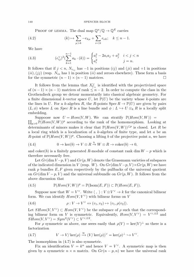
140 SPENCER BLOCH
Proof of lemma. The dual map Qn/Q → QE carries
(4.2) (k) �→∑μ>k
−ekμ +∑ν<k
eνk; k ≤ n− 1.
We have
(4.3) (e∨ij)2(
n−1∑k=1
ak · (k)) ={a2i − 2aiaj + a2j i < j < n
a2i j = n.
It follows that if j < n, Neij has −1 in positions (ij) and (ji) and +1 in positions(ii), (jj) (resp. Nin has 1 in position (ii) and zeroes elsewhere). These form a basisfor the symmetric (n− 1)× (n− 1) matrices. �
It follows from the lemma that X∨Γn
is identified with the projectivized spaceof (n− 1)× (n− 1) matrices of rank ≤ n− 2. In order to compute the class in theGrothendieck group we detour momentarily into classical algebraic geometry. Fora finite dimensional k-vector space U , let P(U) be the variety whose k-points arethe lines in U . For a k-algebra R, the R-points SpecR → P(U) are given by pairs(L, φ) where L on Spec R is a line bundle and φ : L ↪→ U ⊗k R is a locally splitembedding.
Suppoose now U = Hom(V,W ). We can stratify P(Hom(V,W )) =∐p>0 P(Hom(V,W ))p according to the rank of the homomorphism. Looking at
determinants of minors makes it clear that P(Hom(V,W ))≤p is closed. Let R bea local ring which is a localization of a k-algebra of finite type, and let a be anR-point of P(Hom(V,W ))p. Choosing a lifting b of the projective point a, we have
(4.4) 0 → ker(b) → V ⊗Rb−→ W ⊗R → coker(b) → 0,
and coker(b) is a finitely generated R-module of constant rank dimW − p which istherefore necessarily free.
LetGr(dimV−p, V ) andGr(p,W ) denote the Grassmann varieties of subspacesof the indicated dimension in V (resp. W ). OnGr(dimV −p, V )×Gr(p,W ) we haverank p bundles E,F given respectively by the pullbacks of the universal quotienton Gr(dimV − p, V ) and the universal subbundle on Gr(p,W ). It follows from theabove discussion that
(4.5) P(Hom(V,W ))p = P(Isom(E,F )) ⊂ P(Hom(E,F )).
Suppose now that W = V ∨. Write 〈 , 〉 : V ⊗V ∨ → k for the canonical bilinearform. We can identify Hom(V, V ∨) with bilinear forms on V
(4.6) ρ : V → V ∨ ↔ (v1, v2) �→ 〈v1, ρ(v2)〉.Let SHom(V, V ∨) ⊂ Hom(V, V ∨) be the subspace of ρ such that the correspond-ing bilinear form on V is symmetric. Equivalently, Hom(V, V ∨) = V ∨,⊗2 andSHom(V, V ∨) = Sym2(V ∨) ⊂ V ∨,⊗2.
For ρ symmetric as above, one seees easily that ρ(V ) = ker(V )⊥ so there is afactorization
(4.7) V → V/ ker(ρ)∼=−→ (V/ ker(ρ))∨ = ker(ρ)⊥ ↪→ V ∨.
The isomorphism in (4.7) is also symmetric.Fix an identification V = kn and hence V = V ∨. A symmetric map is then
given by a symmetric n × n matrix. On Gr(n − p, n) we have the universal rank

MOTIVES ASSOCIATED TO SUMS OF GRAPHS 141
p quotient Q = kn ⊗ OGr/K, and also the rank p perpendicular space K⊥ to theuniversal subbundle K. Note K⊥ ∼= Q∨. It follows that
(4.8) P(SHom(kn, kn))p ∼= P(SHom(Q,Q∨))p ⊂ P(SHom(Q,Q∨)).
This is a fibre bundle overGr(n−p, n) with fibre P(Hom(kp, kp))p, the projectivizedspace of symmetric p× p invertible matrices.
We can now compute [X∨Γn
] as follows. Write c(n, p) = [P(SHom(kn, kn))p].We have the following relations:
c(n, 1) = [Pn−1];
n∑p=1
c(n, p) = [P(n+12 )−1];(4.9)
c(n, p) = [Gr(n− p, n)] · c(p, p)(4.10)
[X∨Γn
] =n−2∑p=1
c(n− 1, p)(4.11)
Here (4.10) follows from (4.8). It is easy to see that these formulas lead to anexpression for [X∨
Γn] as a polynomial in the [PN ] and [Gr(n− p− 1, n− 1)] (though
the precise form of the polynomial seems complicated). To finish the proof of theproposition, we have to show that [Gr(a, b)] ∈ Z[A1
k]. Fix a splitting kb = kb−a⊕ka.Stratify Gr(a, b) =
∐ap=0 Gr(a, b)p where
(4.12) Gr(a, b)p =
{V ⊂ kb−a ⊕ ka | dim(V ) = a, Image(V → ka) has rank p} =
{(X,Y, f) | X ⊂ kb−a, Y ⊂ ka, f : Y → X}
where dimX = a− p, dim(Y ) = p. This is a fibration over Gr(b− a− p, b− a)×Gr(p, a) with fibre Ap(b−a−p). By induction, we may assume [Gr(b− a− p, b− a)×Gr(p, a)] ∈ Z[A1
k]. Since the class in the Grothendieck group of a Zariski locallytrivial fibration is the class of the base times the class of the fibre, we conclude[Gr(a, b)p] ∈ Z[A1
k], completing the proof. �
In fact, we will need somewhat more.
Lemma 4.3. Let Γ be a graph.(i) Let e0 ∈ Γ be an edge. Define Γ′ = Γ ∪ ε, the graph obtained from Γ by addingan edge ε with ∂ε = ∂e0. Then X∨
Γ′ is a cone over X∨Γ .
(ii) Define Γ′ = Γ ∪ ε where ε is a tadpole, i.e. ∂ε = 0. Then X∨Γ′ is a cone over
X∨Γ .
Proof. We prove (i). The proof of (ii) is similar and is left for the reader.Let E, V be the edges and vertices of Γ. We have a diagram
(4.13)
QE ∂−−−−→ QV⏐⏐� ∥∥∥QE ⊕Q · ε ∂−−−−→ QV
Dualizing and playing our usual game of interpreting edges as functionals onImage(∂)∨ ∼= QV /Q, we see that ε∨ = e∨0 . Fix a basis for QV /Q so the (e∨)2
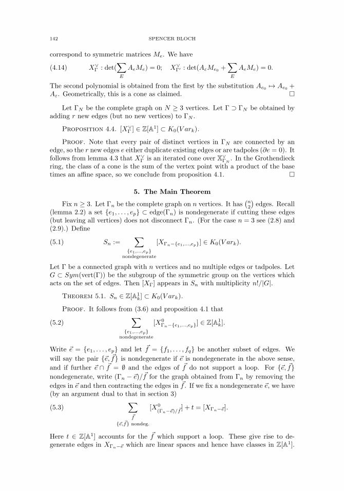
142 SPENCER BLOCH
correspond to symmetric matrices Me. We have
(4.14) X∨Γ : det(
∑E
AeMe) = 0; X∨Γ′ : det(AεMe0 +
∑E
AeMe) = 0.
The second polynomial is obtained from the first by the substitution Ae0 �→ Ae0 +Aε. Geometrically, this is a cone as claimed. �
Let ΓN be the complete graph on N ≥ 3 vertices. Let Γ ⊃ ΓN be obtained byadding r new edges (but no new vertices) to ΓN .
Proposition 4.4. [X∨Γ ] ∈ Z[A1] ⊂ K0(V ark).
Proof. Note that every pair of distinct vertices in ΓN are connected by anedge, so the r new edges e either duplicate existing edges or are tadpoles (∂e = 0). Itfollows from lemma 4.3 that X∨
Γ is an iterated cone over X∨ΓN
. In the Grothendieckring, the class of a cone is the sum of the vertex point with a product of the basetimes an affine space, so we conclude from proposition 4.1. �
5. The Main Theorem
Fix n ≥ 3. Let Γn be the complete graph on n vertices. It has(n2
)edges. Recall
(lemma 2.2) a set {e1, . . . , ep} ⊂ edge(Γn) is nondegenerate if cutting these edges(but leaving all vertices) does not disconnect Γn. (For the case n = 3 see (2.8) and(2.9).) Define
(5.1) Sn :=∑
{e1,...,ep}nondegenerate
[XΓn−{e1,...,ep}] ∈ K0(V ark).
Let Γ be a connected graph with n vertices and no multiple edges or tadpoles. LetG ⊂ Sym(vert(Γ)) be the subgroup of the symmetric group on the vertices whichacts on the set of edges. Then [XΓ] appears in Sn with multiplicity n!/|G|.
Theorem 5.1. Sn ∈ Z[A1k] ⊂ K0(V ark).
Proof. It follows from (3.6) and proposition 4.1 that
(5.2)∑
{e1,...,ep}nondegenerate
[X0Γn−{e1,...,ep}] ∈ Z[A1
k].
Write �e = {e1, . . . , ep} and let �f = {f1, . . . , fq} be another subset of edges. We
will say the pair {�e, �f} is nondegenerate if �e is nondegenerate in the above sense,
and if further �e ∩ �f = ∅ and the edges of �f do not support a loop. For {�e, �f}nondegenerate, write (Γn − �e)/�f for the graph obtained from Γn by removing the
edges in �e and then contracting the edges in �f . If we fix a nondegenerate �e, we have(by an argument dual to that in section 3)
(5.3)∑�f
{�e,�f} nondeg.
[X0(Γn−�e)/�f
] + t = [XΓn−�e].
Here t ∈ Z[A1] accounts for the �f which support a loop. These give rise to de-generate edges in XΓn−�e which are linear spaces and hence have classes in Z[A1].

MOTIVES ASSOCIATED TO SUMS OF GRAPHS 143
Summing now over both �e and �f , we conclude
(5.4) Sn ≡∑{�e,�f}
nondegen.
[X0(Γn−�e)/�f
] mod Z[A1].
Note that if �e, �f are disjoint and �f does not support a loop, then �e is nondegen-
erate in Γn if and only if it is nondegenerate in Γn/�f . This means we can rewrite(5.4)
(5.5) Sn ≡∑�f
∑�e⊂Γn/�fnondegen.
[X0(Γn/�f)−�e
].
Let �f = {f1, . . . , fq} and assume it does not support a loop. Then Γn/�f hasn− q vertices, and every pair of distinct vertices is connected by at least one edge.
This means we may embed Γn−q ⊂ Γn/�f and think of Γn/�f as obtained from Γn−q
by adding duplicate edges and tadpoles. We then apply proposition 4.4 to concludethat [X∨
Γn/�f] ∈ Z[A1
k]. Now arguing as in (3.6) we conclude
(5.6)∑
�e⊂Γn/�fnondegen.
[X0(Γn/�f)−�e
] ∈ Z[A1k]
Finally, plugging into (5.5) we get Sn ∈ Z[A1] as claimed. �
References
[1] Aluffi, P., and Marcolli, M., Feynman Motives of Banana Graphs, arXiv:0807.1690v2 [hep-th][2] Belkale, P., and Brosnan, P., Matroids, motives and a conjecture on Kontsevich, Duke Math.
Journal, Vol. 116 (2003) 147-188.[3] Bloch, S, Esnault, H., and Kreimer, D., On Motives Associated to Graph Polynomials, Comm.
Math. Phys. 267 (2006), 181-225.
[4] Broadhurst, D.J., and Kreimer, D., Association of multiple zeta values with positive knotsvia Feynman diagrams up to 9 loops, Phys. Lett.B 393 (1997) 403.
[5] Stanley, R., Spanning Trees and a Conjecture of Kontsevich, Annals of Combinatorics2(1999), 351-363.
Dept. of Mathematics, University of Chicago, Chicago, IL 60637, USA
E-mail address: [email protected]

Clay Mathematics Proceedings
Double shuffle relations and renormalization of multiple zetavalues
Li Guo, Sylvie Paycha, Bingyong Xie, and Bin Zhang
Abstract. In this paper we present some of the recent progresses in multiplezeta values (MZVs). We review the double shuffle relations for convergentMZVs and summarize generalizations of the sum formula and the decompo-sition formula of Euler for MZVs. We then discuss how to apply methodsborrowed from renormalization in quantum field theory and from pseudodif-ferential calculus to partially extend the double shuffle relations to divergentMZVs.
1. Introduction
The purpose of this paper is to give a survey of recent developments in multiplezeta values (MZVs). We emphasize on the double shuffle relations which under-lie the algebraic relations among the convergent MZVs, and on renormalizationmethods that aim to extend the double shuffle relations to MZVs outside of theconvergent range of the nested sums defining MZVs. We also provide backgroundon double shuffle relations and renormalization, as well as the closely related Rota-Baxter algebras and some analytic tools in pseudodifferential calculus in view ofrenormalization.
1.1. Double shuffle relations and Euler’s formulas. A multiple zetavalue (MZV) is the special value of the complex valued function
ζ(s1, · · · , sk) =∑
n1>···>nk�1
1
ns11 · · ·nsk
k
at positive integers s1, · · · , sk with s1 � 2 to insure the convergence of the nestedsum. MZVs are natural generalizations of the Riemann zeta values ζ(s) to multiplevariables. The two variable case (double zeta values) was already studied by Euler.
MZVs in the general case were introduced in the 1990s with motivations fromnumber theory [70], combinatorics [40] and quantum field theory [11]. Since thenthe subject has turned into an active area of research that involves many areas ofmathematics and mathematical physics [13]. Its number theoretic significance canbe seen from the fact that all MZVs are periods of mixed Tate motives over Z andthe conjecture that all periods of mixed Tate motives are rational combinations ofMZVs [25, 27, 69].
c© 2010 Li Guo, Sylvie Paycha, Bingyong Xie and Bin Zhang
145
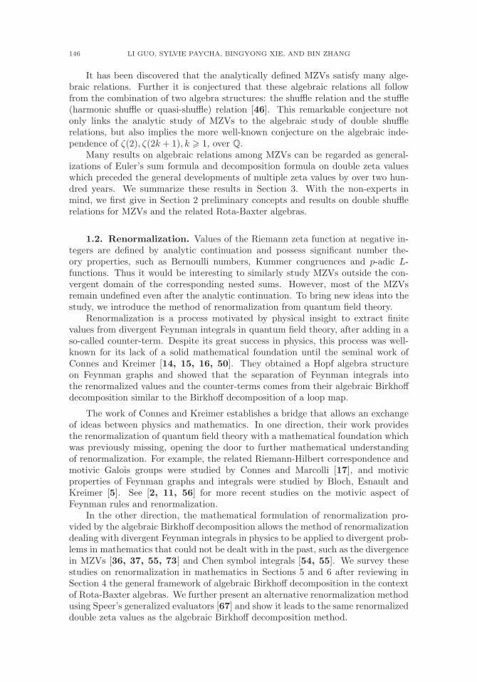
146 LI GUO, SYLVIE PAYCHA, BINGYONG XIE, AND BIN ZHANG
It has been discovered that the analytically defined MZVs satisfy many alge-braic relations. Further it is conjectured that these algebraic relations all followfrom the combination of two algebra structures: the shuffle relation and the stuffle(harmonic shuffle or quasi-shuffle) relation [46]. This remarkable conjecture notonly links the analytic study of MZVs to the algebraic study of double shufflerelations, but also implies the more well-known conjecture on the algebraic inde-pendence of ζ(2), ζ(2k + 1), k � 1, over Q.
Many results on algebraic relations among MZVs can be regarded as general-izations of Euler’s sum formula and decomposition formula on double zeta valueswhich preceded the general developments of multiple zeta values by over two hun-dred years. We summarize these results in Section 3. With the non-experts inmind, we first give in Section 2 preliminary concepts and results on double shufflerelations for MZVs and the related Rota-Baxter algebras.
1.2. Renormalization. Values of the Riemann zeta function at negative in-tegers are defined by analytic continuation and possess significant number the-ory properties, such as Bernoulli numbers, Kummer congruences and p-adic L-functions. Thus it would be interesting to similarly study MZVs outside the con-vergent domain of the corresponding nested sums. However, most of the MZVsremain undefined even after the analytic continuation. To bring new ideas into thestudy, we introduce the method of renormalization from quantum field theory.
Renormalization is a process motivated by physical insight to extract finitevalues from divergent Feynman integrals in quantum field theory, after adding in aso-called counter-term. Despite its great success in physics, this process was well-known for its lack of a solid mathematical foundation until the seminal work ofConnes and Kreimer [14, 15, 16, 50]. They obtained a Hopf algebra structureon Feynman graphs and showed that the separation of Feynman integrals intothe renormalized values and the counter-terms comes from their algebraic Birkhoffdecomposition similar to the Birkhoff decomposition of a loop map.
The work of Connes and Kreimer establishes a bridge that allows an exchangeof ideas between physics and mathematics. In one direction, their work providesthe renormalization of quantum field theory with a mathematical foundation whichwas previously missing, opening the door to further mathematical understandingof renormalization. For example, the related Riemann-Hilbert correspondence andmotivic Galois groups were studied by Connes and Marcolli [17], and motivicproperties of Feynman graphs and integrals were studied by Bloch, Esnault andKreimer [5]. See [2, 11, 56] for more recent studies on the motivic aspect ofFeynman rules and renormalization.
In the other direction, the mathematical formulation of renormalization pro-vided by the algebraic Birkhoff decomposition allows the method of renormalizationdealing with divergent Feynman integrals in physics to be applied to divergent prob-lems in mathematics that could not be dealt with in the past, such as the divergencein MZVs [36, 37, 55, 73] and Chen symbol integrals [54, 55]. We survey thesestudies on renormalization in mathematics in Sections 5 and 6 after reviewing inSection 4 the general framework of algebraic Birkhoff decomposition in the contextof Rota-Baxter algebras. We further present an alternative renormalization methodusing Speer’s generalized evaluators [67] and show it leads to the same renormalizeddouble zeta values as the algebraic Birkhoff decomposition method.

MULTIPLE ZETA VALUES 147
We hope our paper will expose this active area to a wide range of audience andpromote its further study, to gain a more thorough understanding of the doubleshuffle relations for convergent MZVs and to establish a systematical renormaliza-tion theory for the divergent MZVs. One topic that we find of interest is to comparethe various renormalization methods presented in this paper from an abstract pointof view in terms of a renormalization group yet to be described in this context, againmotivated by the study in quantum field theory. With implications back to physicsin mind, we note that MZVs offer a relatively handy and tractable field of experi-ment for such issues when compared with the very complicated Feynman integralcomputations.
Acknowledgements: L. Guo acknowledges the support from NSF grant DMS-0505643 and thanks JAMI at Johns Hopkins University for its hospitality. S. Paychais grateful to D. Manchon for his comments on a preliminary version of part of thispaper. B. Xie is supported by postdoctoral grant 533149-087 provided by PekingUniversity. B. Zhang acknowledges the support from NSFC grant 10631050. Theauthors also thank the referee for detailed comments.
2. Double shuffle relations for convergent multiple zeta values
All rings and algebras in this paper are assumed to be unitary unless otherwisespecified. Let k be a commutative ring whose identity is denoted by 1.
2.1. Rota-Baxter algebras. Let λ ∈ k be fixed. A unitary (resp. nonuni-tary) Rota–Baxter k-algebra (RBA) of weight λ is a pair (R,P ) in which Ris a unitary (resp. nonunitary) k-algebra and P : R → R is a k-linear map suchthat
(1) P (x)P (y) = P (xP (y)) + P (P (x)y) + λP (xy), ∀x, y ∈ R.
In some references such as [55], the notation θ = −λ is used.We will mainly consider the following Rota-Baxter operators in this paper.
See [19, 30, 64] for other examples.
Example 2.1. (The integration operator) Define the integration operator
(2) I(f)(x) =
∫ x
0
f(t)dt
on the algebra C[0,∞) of continuous functions f(x) on [0,∞). Then it follows fromthe integration by parts formula that I is a Rota-Baxter operator of weight 0 [4].
Example 2.2. (The summation operator) Consider the summation oper-ator [75]
P (f)(x) :=∑n�1
f(x+ n).
Under certain convergency conditions, such as f(x) = O(x−2) and g(x) = O(x−2),P (f)(x) and P (g)(x) define absolutely convergent series and we have
P (f)(x)P (g)(x) =∑m�1
f(x+m)∑n�1
g(x+ n)
=∑
n>m�1
f(x+m)g(x+ n) +∑
m>n�1
f(x+m)g(x+ n)(3)
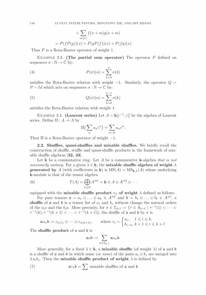
148 LI GUO, SYLVIE PAYCHA, BINGYONG XIE, AND BIN ZHANG
+∑m�1
f(x+m)g(x+m)
= P (fP (g))(x) + P (gP (f))(x) + P (fg)(x).
Thus P is a Rota-Baxter operator of weight 1.
Example 2.3. (The partial sum operator) The operator P defined onsequences σ : N → C by:
(4) P (σ)(n) =
n∑k=0
σ(k)
satisfies the Rota-Baxter relation with weight −1. Similarly, the operator Q =P − Id which acts on sequences σ : N → C by:
(5) Q(σ)(n) =
n−1∑k=0
σ(k)
satisfies the Rota-Baxter relation with weight 1.
Example 2.4. (Laurent series) Let A = k[ε−1, ε]] be the algebra of Laurentseries. Define Π : A → A by
Π(∑
n
anεn)=∑n<0
anεn.
Then Π is a Rota-Baxter operator of weight −1.
2.2. Shuffles, quasi-shuffles and mixable shuffles. We briefly recall theconstruction of shuffle, stuffle and quasi-shuffle products in the framework of mix-able shuffle algebras [32, 33].
Let k be a commutative ring. Let A be a commutative k-algebra that is notnecessarily unitary. For a given λ ∈ k, the mixable shuffle algebra of weight λgenerated by A (with coefficients in k) is MS(A) = MSk,λ(A) whose underlyingk-module is that of the tensor algebra
(6) T (A) =⊕k≥0
A⊗k = k⊕A⊕A⊗2 ⊕ · · ·
equipped with the mixable shuffle product �λ of weight λ defined as follows.For pure tensors a = a1 ⊗ . . . ⊗ ak ∈ A⊗k and b = b1 ⊗ . . . ⊗ b� ∈ A⊗�, a
shuffle of a and b is a tensor list of ai and bj without change the natural ordersof the ais and the bjs. More precisely, for σ ∈ Σk,� := {τ ∈ Sk+� | τ−1(1) < · · · <τ−1(k), τ−1(k + 1) < · · · < τ−1(k + �)}, the shuffle of a and b by σ is
aXσb := cσ(1) ⊗ · · · ⊗ cσ(k+�), where ci =
{ai, 1 � i � k,bi−k, k + 1 � i � k + �
The shuffle product of a and b is
aXb :=∑
σ∈Σk,�
aXσb.
More generally, for a fixed λ ∈ k, a mixable shuffle (of weight λ) of a and b
is a shuffle of a and b in which some (or none) of the pairs ai ⊗ bj are merged intoλ aibj . Then the mixable shuffle product of weight λ is defined by
(7) a�λb =∑
mixable shuffles of a and b
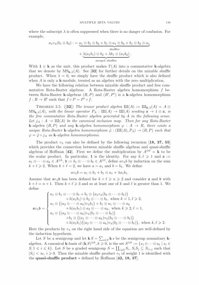
MULTIPLE ZETA VALUES 149
where the subscript λ is often suppressed when there is no danger of confusion. Forexample,
a1�λ(b1 ⊗ b2) : = a1 ⊗ b1 ⊗ b2 + b1 ⊗ a1 ⊗ b2 + b1 ⊗ b2 ⊗ a1︸ ︷︷ ︸shuffles
+λ(a1b1)⊗ b2 + λb1 ⊗ (a1b2)︸ ︷︷ ︸merged shuffles
.
With 1 ∈ k as the unit, this product makes T (A) into a commutative k-algebrathat we denote by MSk,λ(A). See [32] for further details on the mixable shuffleproduct. When λ = 0, we simply have the shuffle product which is also definedwhen A is only a k-module, treated as an algebra with the zero multiplication.
We have the following relation between mixable shuffle product and free com-mutative Rota-Baxter algebras. A Rota-Baxter algebra homomorphism f be-tween Rota-Baxter k-algebras (R,P ) and (R′, P ′) is a k-algebra homomorphismf : R → R′ such that f ◦ P = P ′ ◦ f .
Theorem 2.5. ([32]) The tensor product algebra X(A) := Xk,λ(A) = A ⊗MSk,λ(A), with the linear operator PA : X(A) → X(A) sending a → 1 ⊗ a, isthe free commutative Rota-Baxter algebra generated by A in the following sense.Let jA : A → X(A) be the canonical inclusion map. Then for any Rota-Baxterk-algebra (R,P ) and any k-algebra homomorphism ϕ : A → R, there exists aunique Rota-Baxter k-algebra homomorphism ϕ : (X(A), PA) → (R,P ) such thatϕ = ϕ ◦ jA as k-algebra homomorphisms.
The product �λ can also be defined by the following recursion [18, 37, 55]which provides the connection between mixable shuffle algebras and quasi-shufflealgebras of Hoffman [42]. First we define the multiplication by A⊗0 = k to bethe scalar product. In particular, 1 is the identity. For any k, � � 1 and a :=a1 ⊗ · · · ⊗ ak ∈ A⊗k, b := b1 ⊗ · · · ⊗ b� ∈ A⊗�, define a�λb by induction on the sumk + � � 2. When k + � = 2, we have a = a1 and b = b1. We define
a�λb = a1 ⊗ b1 + b1 ⊗ a1 + λa1b1.
Assume that a�λb has been defined for k + � � n � 2 and consider a and b withk + � = n+ 1. Then k + � � 3 and so at least one of k and � is greater than 1. Wedefine
a�λb =
⎧⎪⎪⎪⎪⎪⎪⎪⎪⎨⎪⎪⎪⎪⎪⎪⎪⎪⎩
a1 ⊗ b1 ⊗ · · · ⊗ b� + b1 ⊗(a1�λ(b2 ⊗ · · · ⊗ b�)
)+λ(a1b1)⊗ b2 ⊗ · · · ⊗ b�, when k = 1, � � 2,
a1 ⊗((a2 ⊗ · · · ⊗ ak)�λb1
)+ b1 ⊗ a1 ⊗ · · · ⊗ ak
+λ(a1b1)⊗ a2 ⊗ · · · ⊗ ak, when k � 2, � = 1,a1 ⊗
((a2 ⊗ · · · ⊗ ak)�λ(b1 ⊗ · · · ⊗ b�)
)+b1 ⊗
((a1 ⊗ · · · ⊗ ak)�λ(b2 ⊗ · · · ⊗ b�)
)+λ(a1b1)
((a2 ⊗ · · · ⊗ ak)�λ(b2 ⊗ · · · ⊗ b�)
), when k, � � 2.
Here the products by �λ on the right hand side of the equation are well-defined bythe induction hypothesis.
Let S be a semigroup and let kS =∑
s∈S k s be the semigroup nonunitary k-
algebra. A canonical k-basis of (kS)⊗k, k � 0, is the set S⊗k := {s1⊗· · ·⊗sk | si ∈S, 1 � i � k}. Let S be a graded semigroup S =
∐i�0 Si, SiSj ⊆ Si+j such that
|Si| < ∞, i � 0. Then the mixable shuffle product �1 of weight 1 is identified withthe quasi-shuffle product ∗ defined by Hoffman [42, 18, 37].

150 LI GUO, SYLVIE PAYCHA, BINGYONG XIE, AND BIN ZHANG
Notation 2.6. To simplify the notation and to be consistent with the usualnotations in the literature on multiple zeta values, we will identify s1⊗· · ·⊗sk withthe concatenation s1 · · · sk unless there is a danger of confusion. We also denotethe weight 1 mixable shuffle product �1 by ∗ and denote the corresponding mixablealgebra MSk,1(A) by H∗
A. Similarly, when A is taken to be a k-module, we denote
the weight zero mixable shuffle algebra MSk,0(A) by HX
A .
Yet another interpretation of the mixable shuffle or quasi-shuffle product can begiven in terms of order preserving maps that are called stuffle in the study of MZVsbut could be traced back to Cartier’s work [12] on free commutative Rota-Baxteralgebras.
For positive integers k and �, denote [k] = {1, · · · , k} and [k + 1, k + �] ={k + 1, · · · , k + �}. Define
(8) Ik,� =
{(ϕ, ψ)
∣∣∣ ϕ : [k] → [k + �], ψ : [�] → [k + �] are order preservinginjective maps and im(ϕ) � im(ψ) = [k + �]
}
Let a ∈ A⊗k, b ∈ A⊗� and (ϕ, ψ) ∈ Ik,�. We define aX(ϕ,ψ)b to be the tensor whosei-th factor is
(9) (aX(ϕ,ψ)b)i =
{aj if i = ϕ(j)bj if i = ψ(j)
= aϕ−1(i)bψ−1(i), 1 � i � k + �,
with the convention that a∅ = b∅ = 1. Then we have
(10) aXb =∑
(ϕ,ψ)∈Ik,�
aX(ϕ,ψ)b.
More generally, for 0 � r � min(k, �), define
Ik,�,r=
{(ϕ, ψ)
∣∣∣ϕ : [k] → [k + �− r], ψ : [�] → [k + �− r] are order preservinginjective maps and im(ϕ) ∪ im(ψ) = [k + �− r]
}
Clearly, Ik,�,0 = Ik,�. Let a ∈ A⊗k, b ∈ A⊗� and (ϕ, ψ) ∈ Ik,�,r. We define aX(ϕ,ψ)b
to be the tensor whose i-th factor is
(aX(ϕ,ψ)b)i =
⎧⎨⎩
aj if i = ϕ(j), i /∈ imψbj if i = ψ(j), i /∈ imϕajbj′ if i = ϕ(j), i = ψ(j′)
⎫⎬⎭ = aϕ−1(i)bψ−1(i), 1 � i � k + �− r,
with the convention that a∅ = b∅ = 1. Then we have [32, 36]
(11) a �λ b =
min(k,�)∑r=0
λr( ∑
(ϕ,ψ)∈Ik,�,r
aX(ϕ,ψ)b
).
In particular,
a ∗ b =
min(k,�)∑r=0
( ∑(ϕ,ψ)∈Ik,�,r
aX(ϕ,ψ)b
)=
∑(ϕ,ψ)∈Ik,�
aX(ϕ,ψ)b
where Ik,� = ∪min(k,�)r=0 Ik,�,r.
Equivalently, let stfl(k, �, r) denote the set of surjective maps from [k + �] to[k + �− r] that preserve the natural orders of [k] and {k + 1, · · · , k + �}. Let
stfl(k, �) =
min(k,�)⋃r=0
stfl(k, �, r).

MULTIPLE ZETA VALUES 151
Then
(12) (a1 ⊗ · · · ⊗ ak) ∗ (ak+1 ⊗ · · · ⊗ ak+�) =∑
π∈stfl(k,�)
cπ1 ⊗ · · · ⊗ cπk+�−r,
where cπi =∏
j∈π−1(i) aj . A connected filtered Hopf algebra is a Hopf algebra
(H,Δ) with k-submodules H(n), n � 0 of H such that
H(n) ⊆ H(n+1), ∪n�0H(n) = H, H(p)H(q) ⊆ H(p+q),
Δ(H(n)) ⊆∑
p+q=n H(p) ⊗H(q), H(0) = k (connectedness).
On the algebra MSk,λ(A) further define
Δ(a1 ⊗ · · · ⊗ an) = 1⊗
(a1 ⊗ · · · ⊗ an) + a1⊗
(a2 ⊗ · · · ⊗ an)
+ · · ·+ (a1 ⊗ · · · an−1)⊗
an + (a1 ⊗ · · · ⊗ an)⊗ 1.(13)
Then Δ extends by linearity to a linear map MSk,λ(A) → MSk,λ(A)⊗
MSk,λ(A).
Theorem 2.7. ([37, 42, 55]) The triple (MSk,λ(A), �λ,Δ), together with theunit u : k ↪→ MSk,λ(A) and the counit ε : MSk,λ(A) → k projecting onto the directsummand k ⊆ MSk,λ(A), equips MSk,λ(A) with the structure of a connected filtered
Hopf algebra with the filtration MS(A)(n) :=∑
i�n A⊗i.
We also have the following easy extension of Hoffman’s isomorphism betweenthe shuffle Hopf algebra and the quasi-shuffle Hopf algebra (see also [18]). Recall
the notation H∗A = MSk,1(A) and H
X
A = MSk,0(A).
Theorem 2.8. ([42, 55]) Let k be a Q-algebra. There is an isomorphism ofHopf algebras :
(14) exp : HX
A∼−→H∗
A.
Hoffman’s isomorphism (14) is built explicitly as follows. Let P(n) be the setof compositions of the integer n, i.e. the set of sequences I = (i1, . . . , ik) of positiveintegers such that i1 + · · · + ik = n. For any u = v1 ⊗ · · · ⊗ vn ∈ T (A) and anycomposition I = (i1, . . . , ik) of n we set:
I[u] := (v1 · · · · · vi1)⊗ (vi1+1 · · · · · vi1+i2)⊗ · · · ⊗ (vi1+···+ik−1+1 · · · · · vn).
Then the isomorphism exp is defined by
expu =∑
I=(i1,··· ,ik)∈P(n)
1
i1! · · · ik!I[u].
Moreover ([42], Lemma 2.4), the inverse log of exp is given by :
log u =∑
I=(i1,··· ,ik)∈P(n)
(−1)n−k
i1 · · · ikI[u].
2.3. Double shuffle of MZVs and related conjectures. A multiple zetavalue (MZV) is defined to be
(15) ζ(s1, · · · , sk) :=∑
n1>···>nk�1
1
ns11 · · ·nsk
k

152 LI GUO, SYLVIE PAYCHA, BINGYONG XIE, AND BIN ZHANG
where si � 1 and s1 > 1 are integers. As is well-known, an MZV has an integralrepresentation due to Kontsevich [51]
(16) ζ(s1, · · · , sk) =∫ 1
0
∫ t1
0
· · ·∫ t|�s|−1
0
dt1f1(t1)
· · ·dt|�s|
f|�s|(t|�s|)
Here |�s| = s1 + · · ·+ sk and
fj(t) =
{1− tj , j = s1, s1 + s2, · · · , s1 + · · ·+ sk,tj , otherwise.
The MZVs spanned the following Q-subspace of R
MZV := Q{ζ(s1, · · · , sk) | si � 1, s1 � 2} ⊆ R.
Since the summation operator in Eq. (15) and the integral operator in Eq. (2)are both Rota-Baxter operators (of weight 1 and 0 respectively) by Example 2.2and Example 2.1, it can be expected that the multiplication of two MZVs followsthe multiplication rule in a free Rota-Baxter algebra and thus in a mixable shufflealgebra. This viewpoint naturally leads to the following double shuffle relations ofMZVs.
For the sum representation of MZVs in Eq. (15), consider the semigroup
Z := {zs | s ∈ Z�1, zs · zt = zs+t, s, t � 1.}With the convention in Notation 2.6, we denote the quasi-shuffle algebra H∗ :=H∗
QZ which contains the subalgebra
H∗0 := Q⊕
(⊕s1>1
Qzs1 · · · zsk).
Then the multiplication rule of MZVs according to their summation representationfollows from the fact that the linear map
(17) ζ∗ : H∗0 → MZV, zs1,··· ,sk �→ ζ(s1, · · · , sk)
is an algebra homomorphism [41, 46].For the integral representation of MZVs in Eq. (16), consider the set X =
{x0, x1}. With the convention in Notation 2.6, we denote the shuffle algebra HX :=HX
QX which contains subalgebras
HX0 := Q⊕ x0H
Xx1 ⊆ HX1 := Q⊕HXx1 ⊆ HX.
Then the multiplication rule of MZVs according to their integral representationsfollows from the statement that the linear map
ζX : HX0 → MZV, xs1−1
0 x1 · · ·xsk−10 x1 �→ ζ(s1, · · · , sk)
is an algebra homomorphism [41, 46].There is a natural bijection of Q-vector spaces (but not algebras)
η : HX1 → H∗, 1 ↔ 1, xs1−1
0 x1 · · ·xsk−10 x1 ↔ zs1,··· ,sk .
that restricts to a bijection of vector spaces η : HX0 → H∗
0. Then the fact that MZVscan be multiplied in two ways is reflected by the commutative diagram
HX0
η ��
ζX ���������� H∗0
ζ∗����������
MZV

MULTIPLE ZETA VALUES 153
Through η, the shuffle product X on HX1 and HX
0 transports to a product X∗on H∗ and H∗
0. That is, for w1, w2 ∈ H∗0, define
(18) w1X∗ w2 := η(η−1(w1)Xη−1(w2)).
Then the double shuffle relation is simply the set
{w1X∗ w2 − w1 ∗ w2 | w1, w2 ∈ H∗0}
and the extended double shuffle relation [46, 63, 75] is the set
(19) {w1X∗ w2 − w1 ∗ w2, z1X∗ w2 − z1 ∗ w2 | w1, w2 ∈ H∗0}.
Theorem 2.9. ([41, 46, 63]) Let IEDS be the ideal of H∗0 generated by the
extended double shuffle relation in Eq. ( 19). Then IEDS is in the kernel of ζ∗.
It is conjectured that IEDS is in fact the kernel of ζ∗. A consequence of thisconjecture is the irrationality of ζ(2n+ 1), n � 1.
3. Generalizations of Euler’s formulas
We begin with stating Euler’s sum and decomposition formulas in Section 3.1.Generalizations of Euler’s sum formula are presented in Section 3.2 and generaliza-tions of Euler’s decomposition formula are presented in Section 3.3.
3.1. Euler’s sum and decomposition formulas. Over two hundred yearsbefore the general study of multiple zeta values was started in the 1990s, Goldbachand Euler had already considered the two variable case, the double zeta values [23,66]
ζ(s1, s2) :=∑
n1>n2�1
1
ns11 ns2
2
.
Among Euler’s major discoveries on double zeta values are his sum formula
n−1∑i=2
ζ(i, n− i) = ζ(n)
expressing one Riemann zeta values as a sum of double zeta values and the de-composition formula
(20) ζ(r)ζ(s) =
s−1∑k=0
(r+k−1
k
)ζ(r+k, s−k)+
r−1∑k=0
(s+k−1
k
)ζ(s+k, r−k), r, s � 2,
expressing the product of two Riemann zeta values as a sum of double zeta values.A major aspect of the study of MZVs is to find algebraic and linear relations
among MZVs, such as Euler’s formulas. Indeed a large part of this study can beviewed as generalizations of Euler’s formulas.
3.2. Generalizations of Euler’s sum formula. Soon after MZVs were in-troduced, Euler’s sum formula was generalized to MZVs [40, 28, 71] as the well-known sum formula, followed by quite a few other generalizations that we will nextsummarize.

154 LI GUO, SYLVIE PAYCHA, BINGYONG XIE, AND BIN ZHANG
3.2.1. Sum formula. The first generalization of Euler’s sum formula is the sumformula conjectured in [40]. Let
(21) I(n, k) = {(s1, · · · , sk) | s1 + · · ·+ sk = n, si � 1, s1 � 2}.For �s = (s1, · · · , sk) ∈ I(n, k), define themultiple zeta star value (or non-strictMZV)
(22) ζ�(s1, · · · , sk) =∑
n1�···�nk�1
1
ns11 · · ·nsk
k
.
Note the subtle difference between the notations ζ∗ in Eq. (17) and ζ� in Eq. (22).
Theorem 3.1. (Sum formula) For positive integers k < n we have
(23)∑
�s∈I(n,k)
ζ(�s) = ζ(n),∑
k∈I(n,k)
ζ�(�s) =
(n−1
k−1
)ζ(n).
The case of k = 3 was proved by M. Hoffman and C. Moen [43] and the generalcase was proved by Zagier [71] with another proof given by Granville [28]. LaterS. Kanemitsu, Y. Tanigawa, M. Yoshimoto [48] gave a proof for the case of k = 2using Mellin transformation.
J.-I. Okuda and K. Ueno [62] gave the following version of the sum formulan∑
k=r
(k−1
r−1
)( ∑�s∈I(n,k)
ζ(�s))=
(n−1
r
)ζ(n)
for n > r � 1 from which they deduced the sum formula Eq. (23).3.2.2. Ohno’s generalized duality theorem. Another formula conjectured in [40]
is the duality formula. To state the duality formula, we need an involution τ onthe set of finite sequences of positive integers whose first element is greater than 1.If
�s = (1 + b1, 1, · · · , 1︸ ︷︷ ︸a1−1
, · · · , 1 + bk, 1, · · · , 1︸ ︷︷ ︸ak−1
),
thenτ (�s) = (1 + ak, 1, · · · , 1︸ ︷︷ ︸
bk−1
, · · · , 1 + a1, 1, · · · , 1︸ ︷︷ ︸b1−1
).
Theorem 3.2. (Duality formula)
ζ(�s) = ζ(τ (�s)).
This formula is an immediate consequence of the integral representation inEq. (16).
Y. Ohno [57] provided a generalization of both the sum formula and the dualityformula.
Theorem 3.3. (Generalized Duality Formula [57]) For any index set �s =(s1, · · · , sk) with s1 � 2, s2 � 1, · · · , sk � 1, and a nonnegative integer �, set
Z(s1, · · · , sk; �) =∑
c1 + · · ·+ ck = �ci � 0
ζ(s1 + c1, · · · , sk + ck).

MULTIPLE ZETA VALUES 155
Then
Z(�s; �) = Z(τ (�s); �).
When � = 0, this is just the duality formula. When �s = (k+1) and � = n−k−1,this becomes the sum formula.
3.2.3. Sum formulas with further conditions on the variables. M. Hoffman andY. Ohno [44] gave a cyclic generalization of the sum formula.
Theorem 3.4. (Cyclic sum formula) For any positive integers s1, · · · , skwith some si � 2,
k∑i=1
ζ(si + 1, si+1, · · · , sk, s1, · · · , si−1)
=∑
{i | si�2}
si−2∑j=0
ζ(si − j, si+1, · · · , sk, s1, · · · , si−1, j + 1).
Y. Ohno and N. Wakabayashi [59] gave a cyclic sum formula for non-strictMZVs and used it to prove the sum formula Eq. (23).
Theorem 3.5. (Cyclic sum formula in the non-strict case) For positiveintegers k < n and (s1, · · · , sk) ∈ I(n, k) we have
(24)k∑
i=1
si−2∑j=0
ζ�(si − j, si+1, · · · , sk, s1, · · · , si−1, j + 1) = nζ(n+ 1),
where the empty sums are zero.
M. Eie, W.-C. Liaw and Y. L. Ong [22] gave a generalization of the sum formulaby allowing a more general form in the arguments in the MZVs.
Theorem 3.6. For all positive integers n, k with n > k, and a nonnegativeinteger p, ∑
s1 + · · ·+ sk = ns1 � 2
ζ(s1, · · · , sk, {1}p) =∑
c1 + · · ·+ cp+1 = n+ pc1 � n− k + 1
ζ(c1, · · · , cp+1).
When p = 0, this becomes the sum formula.
Y. Ohno and D. Zagier [60] studied another kind of sum with certain restrictiveconditions. Let
I(n, k, r) = {(s1, · · · , sk) | si ∈ Z�1, s1 + · · ·+ sk = n,#{si | si � 2} = r}
and put
G(n, k, r) =∑
�s∈I(n,k,r)
ζ(�s).
They studied the associated generating function
Φ(x, y, z) =∑
r�1,k�r,n�k+r
G(n, k, r)xn−k−ryk−rzr−1 ∈ R[x, y, z]
and proved the following
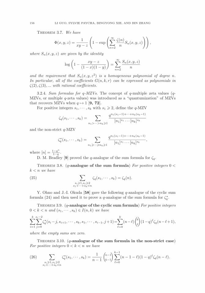
156 LI GUO, SYLVIE PAYCHA, BINGYONG XIE, AND BIN ZHANG
Theorem 3.7. We have
Φ(x, y, z) =1
xy − z
(1− exp
( ∞∑n=2
ζ(n)
nSn(x, y, z)
)),
where Sn(x, y, z) are given by the identity
log
(1− xy − z
(1− x)(1− y)
)=
∞∑n=2
Sn(x, y, z)
n
and the requirement that Sn(x, y, z2) is a homogeneous polynomial of degree n.
In particular, all of the coefficients G(n, k, r) can be expressed as polynomials inζ(2), ζ(3), ... with rational coefficients.
3.2.4. Sum formulas for q-MZVs. The concept of q-multiple zeta values (q-MZVs, or multiple q-zeta values) was introduced as a “quantumization” of MZVsthat recovers MZVs when q �→ 1 [9, 72].
For positive integers s1, · · · , sk with s1 � 2, define the q-MZV
ζq(s1, · · · , sk) =∑
n1>···>nk�1
qn1(s1−1)+···+nk(sk−1)
[n1]s1 · · · [nk]sk
and the non-strict q-MZV
ζ�q (s1, · · · , sk) =∑
n1�···�nk�1
qn1(s1−1)+···+nk(sk−1)
[n1]s1 · · · [nk]sk,
where [n] = 1−qn
1−q .
D. M. Bradley [9] proved the q-analogue of the sum formula for ζq.
Theorem 3.8. (q-analogue of the sum formula) For positive integers 0 <k < n we have
(25)∑
si�1,s1�2s1+···+sk=n
ζq(s1, · · · , sk) = ζq(n).
Y. Ohno and J.-I. Okuda [58] gave the following q-analogue of the cyclic sumformula (24) and then used it to prove a q-analogue of the sum formula for ζ�q .
Theorem 3.9. (q-analogue of the cyclic sum formula) For positive integers0 < k < n and (s1, · · · , sk) ∈ I(n, k) we have
k∑i=1
si−2∑j=0
ζ�q (si−j, si+1, · · · , sk, s1, · · · , si−1, j+1)=
k∑�=0
(n−�)
(k
�
)(1−q)�ζq(n−�+1),
where the empty sums are zero.
Theorem 3.10. (q-analogue of the sum formula in the non-strict case)For positive integers 0 < k < n we have
(26)∑
si�1,s1�2s1+···+sk=n
ζ�q (s1, · · · , sk) =1
n− 1
(n−1
k−1
) k−1∑�=0
(n− 1− �)(1− q)�ζq(n− �).

MULTIPLE ZETA VALUES 157
3.2.5. Weighted sum formulas. Among other directions to generalize Euler’ssum formula, there is the weighted version of Euler’s sum formula recently obtainedby Ohno and Zudilin [61].
Theorem 3.11. (Weighted Euler’s sum formula [61]) For any integer n �2, we have
(27)
n−1∑i=2
2iζ(i, n− i) = (n+ 1)ζ(n).
They applied it to study multiple zeta star values. By the sum formula, Eq. (27)is equivalent to the following equation
(28)
n−1∑i=2
(2i − 1)ζ(i, n− i) = nζ(n).
As a generalization of Eq. (28), two of the authors proved the following
Theorem 3.12. (Weighted sum formula [35]) For integers k � 2 and n �k + 1, we have
nζ(n)
=∑
si�1,s1�2s1+···+sk=n
[2s1−1 + (2s1−1 − 1)
(( k−1∑i=2
2Si−s1−(i−1))+ 2Sk−1−s1−(k−2)
)]ζ(s1, · · · , sk),
where Si = s1 + · · ·+ si for i = 1, · · · , k − 1.
3.3. Generalizations of Euler’s decomposition formula. Unlike the nu-merous generalizations of Euler’s sum formula, no generalization of Euler’s de-composition formula to MZVs, neither proved nor conjectured, had been givenuntil [34] even though Euler’s decomposition formula was recently revisited in con-nection with modular forms [24] and weighted sum formula [61] on weighted sumformula of double zeta values, and was generalized to the product of two q-zetavalues [10, 72].
3.3.1. Euler’s decomposition formula and double shuffle. The first step in gen-eralizing Euler’s decomposition formula is to place it as a special case in a suitablebroader context. In [34], Euler’s decomposition formula was shown to be a specialcase of the double shuffle relation. We give a proof of Euler’s formula in this contextbefore presenting its generalization in the next subsection.
We recall that the extended double shuffle relation is the set
{w1X∗ w2 − w1 ∗ w2, z1X∗ w2 − z1 ∗ w2 | w1, w2 ∈ H∗0}.
Thus the determination of the double shuffle relation amounts to computing thetwo products ∗ and X∗ .
It is straightforward to compute the product ∗, either from its recursive def-inition in Eq. (8) or its explicit interpretation as mixable shuffles in Eq. (7) andstuffles in Eq. (11) or (12). For example, to determine the double shuffle relationfrom multiplying two Riemann zeta values ζ(r) and ζ(s), r, s � 2, one uses theirsum representations and easily gets the quasi-shuffle relation
ζ(r)ζ(s) = ζ(r, s) + ζ(s, r) + ζ(r + s).

158 LI GUO, SYLVIE PAYCHA, BINGYONG XIE, AND BIN ZHANG
On the other hand, computing the product X∗ is more involved as can alreadybe seen from its definition in Eq. (18). One first needs to use their integral rep-resentations to express ζ(r) and ζ(s) as iterated integrals of dimensions r and s,respectively. One then uses the shuffle relation to express the product of these two
iterated integrals as a sum of
(r+s
r
)iterated integrals of dimension r + s. Finally,
these last iterated integrals are translated back to MZVs and give the shuffle relationof ζ(r)ζ(s). As an illustrating example, consider ζ(100)ζ(200). The quasi-shufflerelation is simply ζ(100)ζ(200) = ζ(100, 200)+ ζ(200, 100)+ ζ(300), but the shuffle
relation is a large sum of
(300
100
)shuffles of length (dimension) 300. As we will show
below, an explicit formula for this is precisely Euler’s decomposition formula (20).
Theorem 3.13. For r, s � 2, we have
zrX∗ zs =s−1∑k=0
(r+k−1
k
)zr+kzs−k +
r−1∑k=0
(s+k−1
k
)zs+kzr−k.
Via the algebra homomorphism ζ∗ in Eq. (17) this theorem immediately givesEuler’s decomposition formula. Applying to the above example, we have
ζ(100)ζ(200) =
199∑k=0
(100+k−1
k
)ζ(100 + k, 200− k) +
99∑k=0
(200+k−1
k
)ζ(200 + k, 100− k).
Proof. Following the definition of X∗ in Eq. (18), we have
zrX∗ zs = η(xr−10 x1Xxs−1
0 x1).
So we just need to prove
xr−10 x1Xxs−1
0 x1 =
s−1∑k=0
(r+k−1
k
)xr+k−10 x1x
s−k−10 x1 +
r−1∑k=0
(s+k−1
k
)xs+k−10 x1x
r−k−10 x1
since X∗ (xr+k−10 x1x
s−k−10 x1) = zr+kzs−k and X∗ (x
s+k−10 x1x
r−k−10 x1) = zs+kzr−k.
This has a direct shuffle proof [8]. But we use the description of order preservingmaps of shuffles in order to motivate the general case.
By Eq. (10), we have
xr−10 x1Xxs−1
0 x1 =∑
(ϕ,ψ)∈I(r,s)
xr−10 x1X(ϕ,ψ)x
s−10 x0.
Since ϕ and ψ are order preserving, we have the disjoint union I(r, s) = I(r, s)′ �I(r, s)′′ where
I(r, s)′ = {(ϕ, ψ) ∈ I(r, s) | ψ(s) = r + s}and
I(r, s)′′ = {(ϕ, ψ) ∈ I(r, s) | ϕ(r) = r + s}.Again by the order preserving property, for (ϕ, ψ) ∈ I(r, s)′, we must have ϕ(r) =r + k where k � 0. Thus for such (ϕ, ψ), we have
xr−10 x1X(ϕ,ψ)x
s−10 x1 = xr−1+k
0 x1xs−1−k0 x1
since imϕ � imψ = [r + s]. For fixed k � 0, ϕ(r) = r + k means that there are kelements i1, · · · , ik from [s−1] such that ψ(ij) ∈ [r+k−1] since ψ(s) = r+s. Thusk � s−1 and, since ψ is order preserving, we have {i1, · · · , ik} = [k]. Further there

MULTIPLE ZETA VALUES 159
are
(r+k−1
k
)such ψ’s since ψ([k]) can take any k places in [r + k − 1] in increasing
order and then φ([r]) takes the rest places in increase order. Thus
∑(ϕ,ψ)∈I(r,s)′
xr−10 x1X(ϕ,ψ)x
s−10 x1 =
s−1∑k=0
(r+k−1
k
)xr+k−10 x1x
s−k−10 x1.
By a similar argument, we have
∑(ϕ,ψ)∈I(r,s)′′
xr−10 x1X(ϕ,ψ)x
s−10 x1 =
r−1∑k=0
(s+k−1
k
)xs+k−10 x1x
r−k−10 x1.
This completes the proof. �
3.3.2. Generalizations of Euler’s decomposition formula. In a recent work [34],two of the authors generalized Euler’s decomposition formula in two directions,from the product of one variable functions to that of multiple variables and frommultiple zeta values to multiple polylogarithms.
A multiple polylogarithm value [7, 25, 26] is defined by
Lis1,··· ,sk(z1, · · · , zk) :=∑
n1>···>nk�1
zn11 · · · znk
k
ns11 · · ·nsk
k
where |zi| � 1, si ∈ Z�1, 1 � i � k, and (s1, z1) �= (1, 1). When zi = 1, 1 � i � k,we obtain the multiple zeta values ζ(s1, · · · , sk). With the notation of [7], we have
Lis1,··· ,sk(z1, · · · , zk) = λ( s1, · · · , skb1, · · · , bk
):=
∑n1>n2···>nk�1
(1b1
)n1(b1b2
)n2 · · ·( bk−1
bk
)nk
ns11 ns2
2 · · ·nskk
,
where (b1, · · · , bk) = (z−11 , (z1z2)
−1, · · · , (z1 · · · zk)−1).To state the result, let k and � be positive integers and let Ik,� be as defined in
Eq. (8). Let �r = (r1, · · · , rk) ∈ Zk�1, �s = (s1, · · · , s�) ∈ Z�
�1 and �t = (t1, · · · , tk+�) ∈Zk+��1 with |�r|+ |�s| = |�t|. Here |�r| = r1+ · · ·+rk and similarly for |�s| and |�t|. Denote
Ri = r1 + · · ·+ ri for i ∈ [k], Si = s1 + · · ·+ si for i ∈ [�] and Ti = t1 + · · ·+ ti fori ∈ [k + �]. For (ϕ, ψ) ∈ Ik,� and i ∈ [k + �], define
h(ϕ,ψ),i = h(ϕ,ψ),(�r,�s),i =
{rj if i = ϕ(j)sj if i = ψ(j)
= rϕ−1(i)sψ−1(i),
with the convention that r∅ = s∅ = 1.With these notations, we define
(29) c�t,(ϕ,ψ)�r,�s (i) =
⎧⎪⎪⎪⎪⎪⎪⎪⎪⎪⎨⎪⎪⎪⎪⎪⎪⎪⎪⎪⎩
(ti−1
h(ϕ,ψ),i−1
)if i = 1, if i− 1, i ∈ im(ϕ)or if i− 1, i ∈ im(ψ),(
ti−1
Ti−R|ϕ−1([i])|−S|ψ−1([i])|
)
=
(ti−1
i∑j=1
tj−i∑
j=1
h(ϕ,ψ),j
)otherwise.
For �a ∈ (S1)k and �b ∈ (S1)�, as in Eq. (9), define
(30) �aX(ϕ,ψ)�b = (aϕ−1(1)bψ−1(1), · · · , aϕ−1(k+�)bψ−1(k+�)).
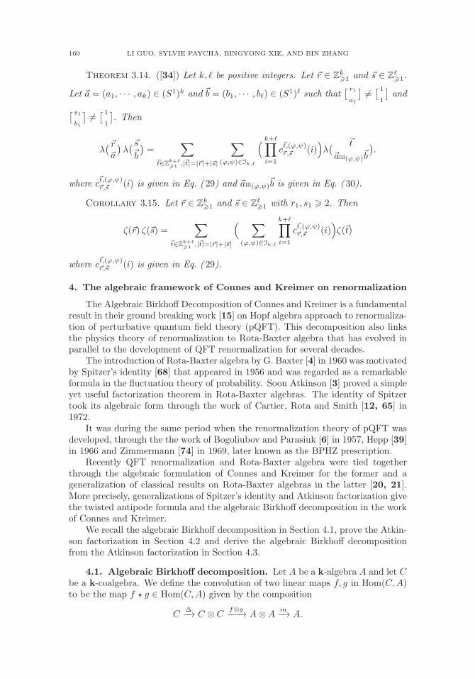
160 LI GUO, SYLVIE PAYCHA, BINGYONG XIE, AND BIN ZHANG
Theorem 3.14. ([34]) Let k, � be positive integers. Let �r ∈ Zk�1 and �s ∈ Z�
�1.
Let �a = (a1, · · · , ak) ∈ (S1)k and �b = (b1, · · · , b�) ∈ (S1)� such that[ r1a1
]�=[ 11
]and
[ s1b1
]�=[ 11
]. Then
λ(�r�a
)λ(�s�b
)=
∑�t∈Z
k+��1 ,|�t|=|�r|+|�s|
∑(ϕ,ψ)∈Ik,�
( k+�∏i=1
c�t,(ϕ,ψ)�r,�s (i)
)λ( �t
�aX(ϕ,ψ)�b
).
where c�t,(ϕ,ψ)�r,�s (i) is given in Eq. ( 29) and �aX(ϕ,ψ)
�b is given in Eq. ( 30).
Corollary 3.15. Let �r ∈ Zk�1 and �s ∈ Z�
�1 with r1, s1 � 2. Then
ζ(�r) ζ(�s) =∑
�t∈Zk+��1 ,|�t|=|�r|+|�s|
( ∑(ϕ,ψ)∈Ik,�
k+�∏i=1
c�t,(ϕ,ψ)�r,�s (i)
)ζ(�t)
where c�t,(ϕ,ψ)�r,�s (i) is given in Eq. ( 29).
4. The algebraic framework of Connes and Kreimer on renormalization
The Algebraic Birkhoff Decomposition of Connes and Kreimer is a fundamentalresult in their ground breaking work [15] on Hopf algebra approach to renormaliza-tion of perturbative quantum field theory (pQFT). This decomposition also linksthe physics theory of renormalization to Rota-Baxter algebra that has evolved inparallel to the development of QFT renormalization for several decades.
The introduction of Rota-Baxter algebra by G. Baxter [4] in 1960 was motivatedby Spitzer’s identity [68] that appeared in 1956 and was regarded as a remarkableformula in the fluctuation theory of probability. Soon Atkinson [3] proved a simpleyet useful factorization theorem in Rota-Baxter algebras. The identity of Spitzertook its algebraic form through the work of Cartier, Rota and Smith [12, 65] in1972.
It was during the same period when the renormalization theory of pQFT wasdeveloped, through the the work of Bogoliubov and Parasiuk [6] in 1957, Hepp [39]in 1966 and Zimmermann [74] in 1969, later known as the BPHZ prescription.
Recently QFT renormalization and Rota-Baxter algebra were tied togetherthrough the algebraic formulation of Connes and Kreimer for the former and ageneralization of classical results on Rota-Baxter algebras in the latter [20, 21].More precisely, generalizations of Spitzer’s identity and Atkinson factorization givethe twisted antipode formula and the algebraic Birkhoff decomposition in the workof Connes and Kreimer.
We recall the algebraic Birkhoff decomposition in Section 4.1, prove the Atkin-son factorization in Section 4.2 and derive the algebraic Birkhoff decompositionfrom the Atkinson factorization in Section 4.3.
4.1. Algebraic Birkhoff decomposition. Let A be a k-algebra A and let Cbe a k-coalgebra. We define the convolution of two linear maps f, g in Hom(C,A)to be the map f � g ∈ Hom(C,A) given by the composition
CΔ−→ C ⊗ C
f⊗g−−−→ A⊗Am−→ A.
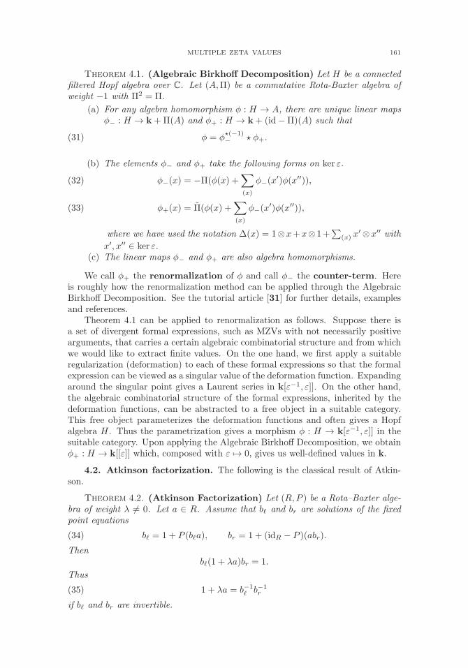
MULTIPLE ZETA VALUES 161
Theorem 4.1. (Algebraic Birkhoff Decomposition) Let H be a connectedfiltered Hopf algebra over C. Let (A,Π) be a commutative Rota-Baxter algebra ofweight −1 with Π2 = Π.
(a) For any algebra homomorphism φ : H → A, there are unique linear mapsφ− : H → k+Π(A) and φ+ : H → k+ (id−Π)(A) such that
(31) φ = φ�(−1)− � φ+.
(b) The elements φ− and φ+ take the following forms on ker ε.
φ−(x) = −Π(φ(x) +∑(x)
φ−(x′)φ(x′′)),(32)
φ+(x) = Π(φ(x) +∑(x)
φ−(x′)φ(x′′)),(33)
where we have used the notation Δ(x) = 1⊗x+x⊗1+∑
(x) x′⊗x′′ with
x′, x′′ ∈ ker ε.(c) The linear maps φ− and φ+ are also algebra homomorphisms.
We call φ+ the renormalization of φ and call φ− the counter-term. Hereis roughly how the renormalization method can be applied through the AlgebraicBirkhoff Decomposition. See the tutorial article [31] for further details, examplesand references.
Theorem 4.1 can be applied to renormalization as follows. Suppose there isa set of divergent formal expressions, such as MZVs with not necessarily positivearguments, that carries a certain algebraic combinatorial structure and from whichwe would like to extract finite values. On the one hand, we first apply a suitableregularization (deformation) to each of these formal expressions so that the formalexpression can be viewed as a singular value of the deformation function. Expandingaround the singular point gives a Laurent series in k[ε−1, ε]]. On the other hand,the algebraic combinatorial structure of the formal expressions, inherited by thedeformation functions, can be abstracted to a free object in a suitable category.This free object parameterizes the deformation functions and often gives a Hopfalgebra H. Thus the parametrization gives a morphism φ : H → k[ε−1, ε]] in thesuitable category. Upon applying the Algebraic Birkhoff Decomposition, we obtainφ+ : H → k[[ε]] which, composed with ε �→ 0, gives us well-defined values in k.
4.2. Atkinson factorization. The following is the classical result of Atkin-son.
Theorem 4.2. (Atkinson Factorization) Let (R,P ) be a Rota–Baxter alge-bra of weight λ �= 0. Let a ∈ R. Assume that b� and br are solutions of the fixedpoint equations
(34) b� = 1 + P (b�a), br = 1 + (idR − P )(abr).
Thenb�(1 + λa)br = 1.
Thus
(35) 1 + λa = b−1� b−1
r
if b� and br are invertible.

162 LI GUO, SYLVIE PAYCHA, BINGYONG XIE, AND BIN ZHANG
We note that the factorization (35) depends on the existence of invertible so-lutions of Eq. (34) that we will address next.
Definition 4.3. A filtered k-algebra is a k-algebra R together with a de-creasing filtration Rn, n � 0, of nonunitary subalgebras such that⋃
n�0
Rn = R, RnRm ⊆ Rn+m.
It immediately follows that R0 = R and each Rn is an ideal of R. A filteredalgebra is called complete if R is a complete metric space with respect to themetric defined by the subsets {Rn}. Equivalently, a filtered k-algebra R with {Rn}is complete if ∩nRn = 0 and if the resulting embedding
R → R := lim←−R/Rn
of R into the inverse limit is an isomorphism.A Rota-Baxter algebra (R,P ) is called complete if there are submodules Rn ⊆
R, n � 0, such that (R,Rn) is a complete algebra and P (Rn) ⊆ Rn.
Theorem 4.4. (Existence and uniqueness of Atkinson factorization)Let (R,P,Rn) be a complete Rota-Baxter algebra. Let a be in R1.
(a) The equations in ( 34) have unique solutions b� and br. Further b� and brare invertible. Hence Atkinson Factorization ( 35) exists.
(b) If λ has no non-zero divisors in R1 and P 2 = −λP (in particular if P 2 =−λP on R), then there are unique c� ∈ 1+P (R) and cr ∈ 1+(idR−P )(R)such that
1 + λa = c�cr.
4.3. From Atkinson factorization to algebraic Birkhoff decomposi-tion. We now derive the Algebraic Birkhoff Decomposition of Connes and Kreimerin Theorem 4.1 from Atkinson Factorization in Theorem 4.4. Adapting the nota-tions in Theorem 4.1, let H be a connected filtered Hopf algebra and let (A,Q) bea commutative Rota-Baxter algebra of weight λ = −1 with Q2 = Q, such as thepair (A,Q) in Theorem 4.1 (see also Example 2.4). The increasing filtration on Hinduces a decreasing filtration Rn = {f ∈ Hom(H,A) | f(Hn−1) = 0}, n � 0 onR := Hom(H,A), making it a complete algebra. Further define
P : R → R, P (f)(x) = Q(f(x)), f ∈ Hom(H,A), x ∈ H.
Then it is easily checked that P is a Rota-Baxter operator of weight −1 and P 2 = P .Thus (R,Rn, P ) is a complete Rota-Baxter algebra.
Now let φ : H → A be a character (that is, an algebra homomorphism).Consider e− φ : H → A. Then
(e− φ)(1H) = e(1H)− φ(1H) = 1H − 1H = 0.
Thus e− φ is in R1. Take e− φ to be our a in Theorem 4.4, we see that there areunique c� ∈ P (R1) and cr ∈ P (R1) such that
φ = c�cr.

MULTIPLE ZETA VALUES 163
Further, by Theorem 4.2, for b� = c−1� , b� = e+P (b� � (e−φ)). Thus for x ∈ ker ε =
ker e, we have
b�(x) = P (b� � (e− φ))(x)
=∑(x)
Q(b�(a(1))(e− φ)(a(2)))
= Q(b�(1H)(e− φ)(x) +
∑(a)
b�(x′)(e− φ)(x′′) + b�(x)(e− φ)(1H)
= −Q(φ(x) +
∑(x)
b�(x′)φ(x′′)
).
In the last equation we have used e(a) = 0, e(a′′) = 0 by definition. Since b�(1H) =1H , we see that b� = φ− in Eq. (32).
Further, we have
cr=c−1� φ=b�φ=−b�(e−φ)+b�=−b�(e−φ)+e+P (b�(e−φ))=e−(id−P )(b�(e−φ)).
With the same computation as for b� above, we see that cr = φ+ in Eq. (33).
5. Heat-kernel type regularization approach to the renormalization ofMZVs
To extend the double shuffle relations to MZVs with non-positive arguments,we have to make sense of the divergent sums defining these MZVs. For this purpose,we adapt the renormalization method from quantum field theory in the algebraicframework of Connes-Kreimer recalled in the last section. We will give three ap-proaches including the approach in this section using a heat-kernel type regulariza-tion, named after a similar process in physics. Since examples and motivations ofthis approach can already be found elsewhere [30, 36, 37], we will be quite sketchyin this section. More details will be given to the two other approaches in Section 6.
5.1. Renormalization of MZVs. Consider the abelian semigroup
(36) M = {[sr
] ∣∣ (s, r) ∈ Z× R>0}
with the multiplication [sr
]·[s′r′]=[s+ s′
r + r′].
With the notation in Section 2.2, we define the Hopf algebra
HM := MSC,1(CM)
with the quasi-shuffle product ∗ and the deconcatenation coproduct Δ in Sec-
tion 2.2. For wi =[siri
]∈ M, i = 1, · · · , k, we use the notations
�w = (w1, . . . , wk) =[s1, . . . , snr1, . . . , rk
]=[�s�r
], where �s = (s1, . . . , sk), �r = (r1, . . . , rk).

164 LI GUO, SYLVIE PAYCHA, BINGYONG XIE, AND BIN ZHANG
For �w =[�s�r
]∈ Mk and ε ∈ C with Re(ε) < 0, define the directional regular-
ized MZV:
(37) Z([�s�r
]; ε) =
∑n1>···>nk>0
en1 r1ε · · · enk rkε
ns11 · · ·nsk
k
It converges for any[�s�r
]and is regarded as the regularization of the formal MZV
(38) ζ(�s) =∑
n1>···>nk>0
1
ns11 · · ·nsk
k
which converges only when si > 0 and s1 > 1. It is related to the multiple polylog-arithm
Lis1,...,sk(z1, . . . , zk) =∑
n1>···>nk>0
zn11 · · · znk
k
ns11 · · ·nsk
k
by a change of variables zi = eriε, 1 � i � k.This regularization defines an algebra homomorphism [36]:
(39) Z : HM → C[T ][[ε, ε−1],
In the same way, for
(40) M− ={[sr
] ∣∣ (s, r) ∈ Z≤0 × R>0
},
Z restricts to an algebra homomorphism
(41) Z : HM− → R := C[[ε, ε−1].
Since both (C[T ][ε−1, ε]],Π) and (C[ε−1, ε]],Π), with Π defined in Example 2.4,are commutative Rota-Baxter algebras with Π2 = Π, we have the decomposition
Z = Z−1− � Z+
by the algebraic Birkhoff decomposition in Theorem 4.1 and obtain
Theorem 5.1. ([36, 37]) The map Z+ : HM → C[T ][[ε]] is an algebra ho-
momorphism which restricts to an algebra homomorphism Z+ : HM− → C[[ε]].
Because of Theorem 5.1, the following definition is valid.
Definition 5.2. For �s = (s1, . . . , sk) ∈ Zk and �r = (r1, . . . , rk) ∈ Rk>0, define
the renormalized directional MZV by
(42) ζ([�s�r
])= lim
ε→0Z+
([�s�r
]; ε).
Here �r is called the direction vector.
As a consequence of Theorem 5.1, we have
Corollary 5.3. The renormalized directional MZVs satisfy the quasi-shufflerelation
(43) ζ([�s�r
])ζ([�s ′
�r ′])
= ζ([�s�r
]∗[�s ′
�r ′]).
Here the right hand side is defined in the same way as in Eq. ( 8).
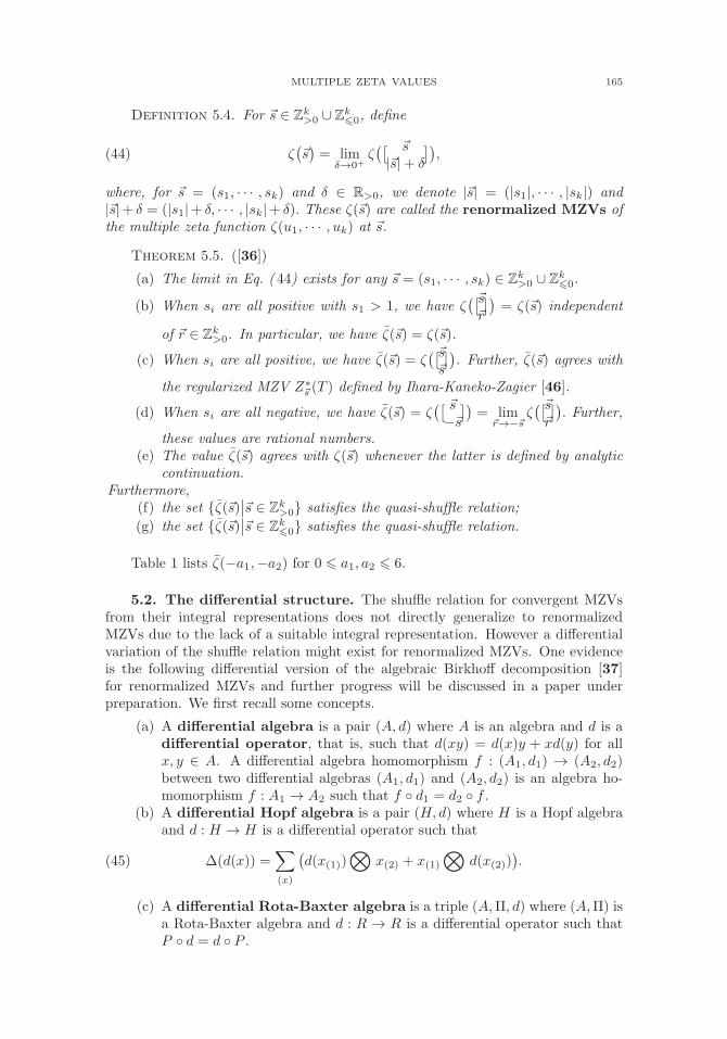
MULTIPLE ZETA VALUES 165
Definition 5.4. For �s ∈ Zk>0 ∪ Zk
�0, define
(44) ζ(�s)= lim
δ→0+ζ([ �s|�s|+ δ
]),
where, for �s = (s1, · · · , sk) and δ ∈ R>0, we denote |�s| = (|s1|, · · · , |sk|) and|�s|+ δ = (|s1|+ δ, · · · , |sk|+ δ). These ζ(�s) are called the renormalized MZVs ofthe multiple zeta function ζ(u1, · · · , uk) at �s.
Theorem 5.5. ([36])
(a) The limit in Eq. ( 44) exists for any �s = (s1, · · · , sk) ∈ Zk>0 ∪ Zk
�0.
(b) When si are all positive with s1 > 1, we have ζ([�s�r
])= ζ(�s) independent
of �r ∈ Zk>0. In particular, we have ζ(�s) = ζ(�s).
(c) When si are all positive, we have ζ(�s) = ζ([�s�s
]). Further, ζ(�s) agrees with
the regularized MZV Z∗�s (T ) defined by Ihara-Kaneko-Zagier [46].
(d) When si are all negative, we have ζ(�s) = ζ([ �s−�s])
= lim�r→−�s
ζ([�s�r
]). Further,
these values are rational numbers.(e) The value ζ(�s) agrees with ζ(�s) whenever the latter is defined by analytic
continuation.Furthermore,
(f) the set {ζ(�s)∣∣�s ∈ Zk
>0} satisfies the quasi-shuffle relation;
(g) the set {ζ(�s)∣∣�s ∈ Zk
�0} satisfies the quasi-shuffle relation.
Table 1 lists ζ(−a1,−a2) for 0 � a1, a2 � 6.
5.2. The differential structure. The shuffle relation for convergent MZVsfrom their integral representations does not directly generalize to renormalizedMZVs due to the lack of a suitable integral representation. However a differentialvariation of the shuffle relation might exist for renormalized MZVs. One evidenceis the following differential version of the algebraic Birkhoff decomposition [37]for renormalized MZVs and further progress will be discussed in a paper underpreparation. We first recall some concepts.
(a) A differential algebra is a pair (A, d) where A is an algebra and d is adifferential operator, that is, such that d(xy) = d(x)y + xd(y) for allx, y ∈ A. A differential algebra homomorphism f : (A1, d1) → (A2, d2)between two differential algebras (A1, d1) and (A2, d2) is an algebra ho-momorphism f : A1 → A2 such that f ◦ d1 = d2 ◦ f .
(b) A differential Hopf algebra is a pair (H, d) where H is a Hopf algebraand d : H → H is a differential operator such that
(45) Δ(d(x)) =∑(x)
(d(x(1))
⊗x(2) + x(1)
⊗d(x(2))
).
(c) A differential Rota-Baxter algebra is a triple (A,Π, d) where (A,Π) isa Rota-Baxter algebra and d : R → R is a differential operator such thatP ◦ d = d ◦ P .
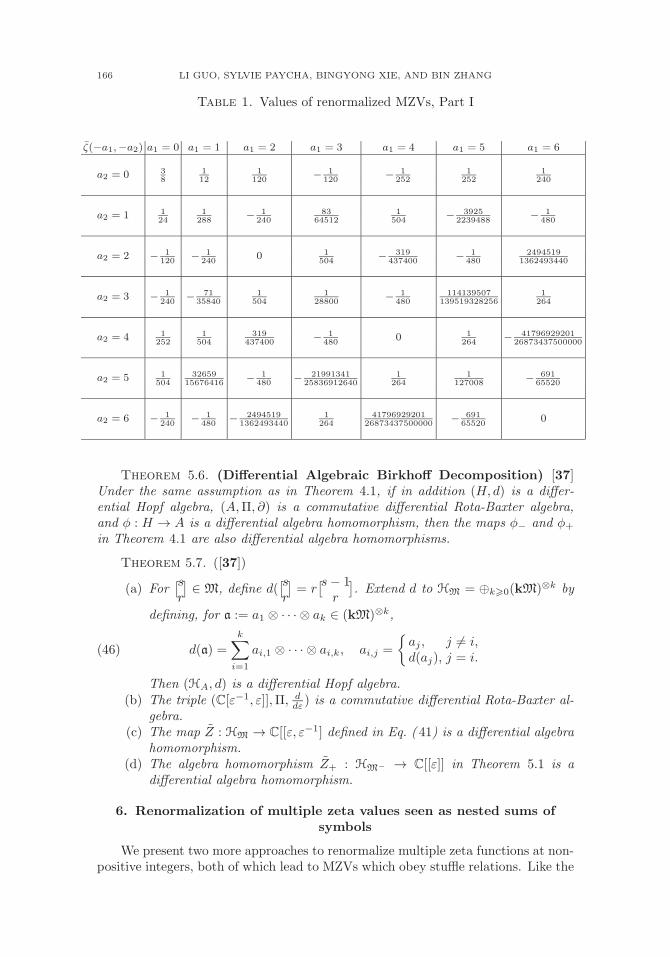
166 LI GUO, SYLVIE PAYCHA, BINGYONG XIE, AND BIN ZHANG
Table 1. Values of renormalized MZVs, Part I
ζ(−a1,−a2) a1 = 0 a1 = 1 a1 = 2 a1 = 3 a1 = 4 a1 = 5 a1 = 6
a2 = 0 38
112
1120
− 1120
− 1252
1252
1240
a2 = 1 124
1288
− 1240
8364512
1504
− 39252239488
− 1480
a2 = 2 − 1120
− 1240
0 1504
− 319437400
− 1480
24945191362493440
a2 = 3 − 1240
− 7135840
1504
128800
− 1480
114139507139519328256
1264
a2 = 4 1252
1504
319437400
− 1480
0 1264
− 4179692920126873437500000
a2 = 5 1504
3265915676416
− 1480
− 2199134125836912640
1264
1127008
− 69165520
a2 = 6 − 1240
− 1480
− 24945191362493440
1264
4179692920126873437500000
− 69165520
0
Theorem 5.6. (Differential Algebraic Birkhoff Decomposition) [37]Under the same assumption as in Theorem 4.1, if in addition (H, d) is a differ-ential Hopf algebra, (A,Π, ∂) is a commutative differential Rota-Baxter algebra,and φ : H → A is a differential algebra homomorphism, then the maps φ− and φ+
in Theorem 4.1 are also differential algebra homomorphisms.
Theorem 5.7. ([37])
(a) For[sr
]∈ M, define d(
[sr
]= r[s− 1
r
]. Extend d to HM = ⊕k�0(kM)⊗k by
defining, for a := a1 ⊗ · · · ⊗ ak ∈ (kM)⊗k,
(46) d(a) =k∑
i=1
ai,1 ⊗ · · · ⊗ ai,k, ai,j =
{aj , j �= i,d(aj), j = i.
Then (HA, d) is a differential Hopf algebra.(b) The triple (C[ε−1, ε]],Π, d
dε ) is a commutative differential Rota-Baxter al-gebra.
(c) The map Z : HM → C[[ε, ε−1] defined in Eq. ( 41) is a differential algebrahomomorphism.
(d) The algebra homomorphism Z+ : HM− → C[[ε]] in Theorem 5.1 is adifferential algebra homomorphism.
6. Renormalization of multiple zeta values seen as nested sums ofsymbols
We present two more approaches to renormalize multiple zeta functions at non-positive integers, both of which lead to MZVs which obey stuffle relations. Like the

MULTIPLE ZETA VALUES 167
renormalization method described in the previous section, they both give rise to ra-tional multiple zeta values at non-positive integers and we check that the two meth-ods yield the same double multiple zeta values at non-positive integer arguments.This presentation is based on joint work of one of the authors with D. Manchon[55] in which multiple zeta functions are viewed as particular instances of nestedsums of symbols and where the algebraic Birkhoff decomposition approach is usedto renormalize multiple zeta functions at poles. Here, we furthermore present analternative renormalization method based on generalized evaluators used in physics[67].
6.1. A class of symbols. For a complex number b, a smooth function f :R − {0} → C is called positively homogeneous of degree b if f(t ξ) = tbf(ξ)for all t > 0 and ξ ∈ R.
The symbols which were originally defined on Rn are now defined on R whichis sufficient for our needs in this paper. We call a smooth function σ : R → C asymbol if there is a real number a such that for any non-negative integer γ, thereis a positive constant Cγ with
|∂γσ(ξ)| ≤ Cγ(1 + |ξ|)a−γ , ∀ξ ∈ R.
For a complex number a and a non-negative integer j, let σa−j : R − {0} → C
be a smooth and positively homogeneous function of degree a − j. We write σ ∼∑∞j=0 σa−j if, for any non-negative integer N and non-negative integer γ, there is
a positive constant Cγ,N such that∣∣∣∣∣∣∂γ
⎛⎝σ(ξ)−
N∑j=0
σa−j(ξ)
⎞⎠∣∣∣∣∣∣ ≤ Cγ,N (1 + |ξ|)Re (a)−N−1−γ , ∀ξ ∈ R− {0},
where Re(a) stands for the real part of a.For any complex number a and any non-negative integer k, a symbol σ : R → C
is called a log-polyhomogeneous of log-type k and order a if
(47) σ(ξ) =
k∑l=0
σl(ξ) logl |ξ|, σl(ξ) ∼
∞∑j=0
σa−j,l(ξ)
with σa−j,l(ξ) positively homogeneous of degree a− j.Let Sa,k denote the linear space over C of log-polyhomogeneous symbols on R
of log-type k and order a. Then we have Sa,k ⊆ Sa,k+1. Let S∗,k denote the linearspan over C of all Sa,k for a ∈ C. Then S∗,0 corresponds to the algebra of classicalsymbols on R. We also define
S∗,∗ :=
∞⋃k=0
S∗,k
which is an algebra for the ordinary product of functions filtered by the log-type[52] since the product of two symbols of log-types k and k′ respectively is of log-type k + k′. The union
⋃a∈Z
⋃∞k=0 S
a,k is a subalgebra of S∗,∗, and⋃
a∈Z Sa,0 is a
subalgebra of S∗,0.Let Pα,k be the algebra of positively supported symbols, i.e. symbols in
Sα,k with support in (0,+∞) so that they are non-zero only at positive arguments.We keep mutatis mutandis the above notations; in particular P∗,0 is a subalgebraof the filtered algebra P∗,∗.
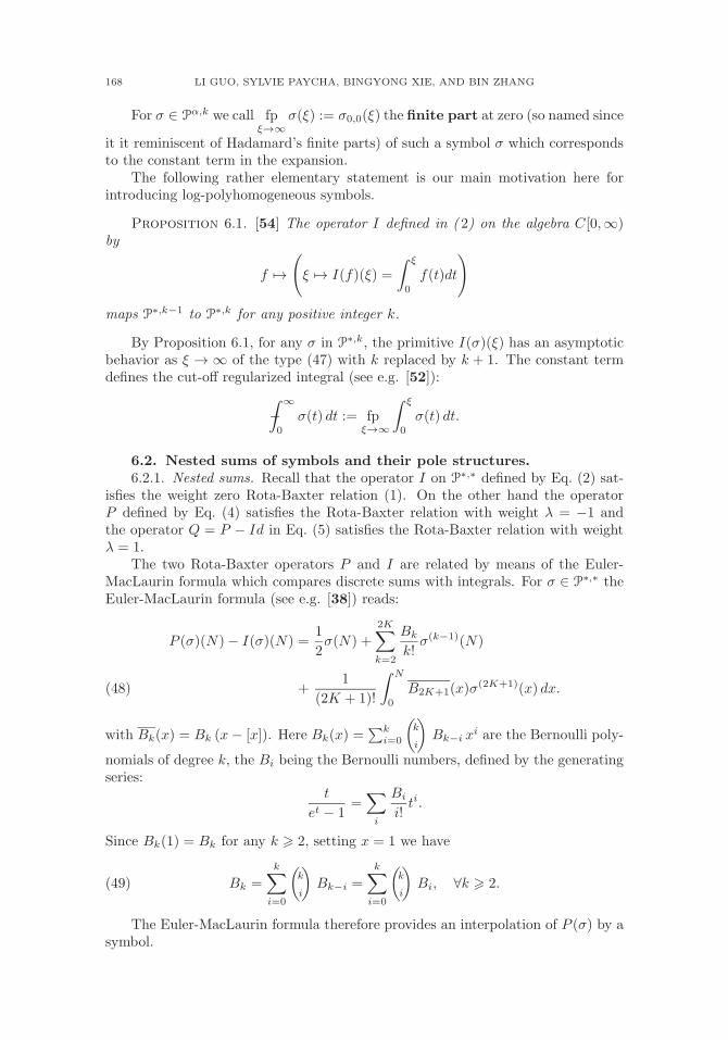
168 LI GUO, SYLVIE PAYCHA, BINGYONG XIE, AND BIN ZHANG
For σ ∈ Pα,k we call fpξ→∞
σ(ξ) := σ0,0(ξ) the finite part at zero (so named since
it it reminiscent of Hadamard’s finite parts) of such a symbol σ which correspondsto the constant term in the expansion.
The following rather elementary statement is our main motivation here forintroducing log-polyhomogeneous symbols.
Proposition 6.1. [54] The operator I defined in ( 2) on the algebra C[0,∞)by
f �→(ξ �→ I(f)(ξ) =
∫ ξ
0
f(t)dt
)
maps P∗,k−1 to P∗,k for any positive integer k.
By Proposition 6.1, for any σ in P∗,k, the primitive I(σ)(ξ) has an asymptoticbehavior as ξ → ∞ of the type (47) with k replaced by k + 1. The constant termdefines the cut-off regularized integral (see e.g. [52]):
−∫ ∞
0
σ(t) dt := fpξ→∞
∫ ξ
0
σ(t) dt.
6.2. Nested sums of symbols and their pole structures.6.2.1. Nested sums. Recall that the operator I on P∗,∗ defined by Eq. (2) sat-
isfies the weight zero Rota-Baxter relation (1). On the other hand the operatorP defined by Eq. (4) satisfies the Rota-Baxter relation with weight λ = −1 andthe operator Q = P − Id in Eq. (5) satisfies the Rota-Baxter relation with weightλ = 1.
The two Rota-Baxter operators P and I are related by means of the Euler-MacLaurin formula which compares discrete sums with integrals. For σ ∈ P∗,∗ theEuler-MacLaurin formula (see e.g. [38]) reads:
P (σ)(N)− I(σ)(N) =1
2σ(N) +
2K∑k=2
Bk
k!σ(k−1)(N)
+1
(2K + 1)!
∫ N
0
B2K+1(x)σ(2K+1)(x) dx.(48)
with Bk(x) = Bk (x− [x]). Here Bk(x) =∑k
i=0
(k
i
)Bk−i x
i are the Bernoulli poly-
nomials of degree k, the Bi being the Bernoulli numbers, defined by the generatingseries:
t
et − 1=∑i
Bi
i!ti.
Since Bk(1) = Bk for any k � 2, setting x = 1 we have
(49) Bk =
k∑i=0
(k
i
)Bk−i =
k∑i=0
(k
i
)Bi, ∀k � 2.
The Euler-MacLaurin formula therefore provides an interpolation of P (σ) by asymbol.

MULTIPLE ZETA VALUES 169
Proposition 6.2. [55] For any σ ∈ Pa,k, the discrete sum P (σ) can be in-terpolated by a symbol P (σ) in Pa+1,k+1 + P0,k+1 (i.e. P (σ)(n) = P (σ)(n) =∑n
k=0 σ(k), ∀n ∈ N) such that
P (σ)− I(σ) ∈ Pa,k.
The operator Q := P − Id : Pa,k → Pa+1,k+1 + P0,k+1 interpolates Q.
By Proposition 6.2, given a symbol σ in Pa,k, the interpolating symbol P (σ) liesin Pa+1,k+1 + P0,k+1. It follows that the discrete sum P (σ)(N) = P (σ)(N) has anasymptotic behavior for large N given by finite linear combinations of expressionsof the type (47) with k replaced by k + 1 and a by a + 1 or 0. Picking the finitepart, for any σ ∈ P∗,∗ we define the following cut-off sum:
(50)
∞−∑0
σ := fpN→∞
P (σ)(N) = fpN→∞
N∑k=0
σ(k),
which extends the ordinary discrete sum∑∞
0 on L1-symbols. If σ has non-integer
order, we have∞−∑0σ = fp
N→∞
∑N+Kk=0 σ(k) for any integer K, so that in particular
∞−∑0σ = fp
N→∞Q(σ)(N) since the operators P and Q only differ by an integer in the
upper bound of the sum.With the help of the interpolation map described in Proposition 6.2, we can
assign to a tensor product σ := σ1 ⊗ · · · ⊗ σk of (positively supported) classicalsymbols, two log-polyhomogeneous symbols defined inductively in the degree k ofthe tensor product, which interpolate the nested iterated sum∑
0�nk�nk−1�···�n2�n1
σ1(n1) · · ·σk(nk) = σ1 P(· · ·σk−2 P
(σk−1 P (σk)
)...),
∑0�nk<nk−1<···<n2<n1
σ1(n1) · · ·σk(nk) = σ1 Q(· · ·σk−2Q
(σk−1 P (σk)
)...).
In the following we will only consider the second class of symbols, including theirregularization, renormalization and application to multiple zeta values. A parallelapproach applies to the first class of symbols with application to non-strict multiplezeta values in Eq. (22) [61, 75].
Theorem 6.3. [55] Given σi ∈ Pαi,0, i = 1, . . . , k, setting σ := σ1 ⊗ · · · ⊗ σk,the function σ defined by:
(51) σ := σ1 Q(· · ·σk−2Q
(σk−1Q(σk)
)...)
which interpolates nested sums in the following way:
σ(n1) =∑
0�nk<nk−1<···<n2<n1
σ1(n1) · · ·σk(nk), ∀n1 ∈ N,
lies in P∗,k−1 that is expressed as linear combinations of (positively supported) sym-bols in Pα1+···+αj+j−1,j−1, j ∈ {1, . . . , k}.
On the ground of this result, we define the cut-off nested discrete sum of atensor product of (positively supported) classical symbols.

170 LI GUO, SYLVIE PAYCHA, BINGYONG XIE, AND BIN ZHANG
Definition 6.4. For σ1, . . . , σk ∈ P∗,0 and σ := σ1 ⊗ · · · ⊗ σk we call
Chen
−∑<
σ :=
∞−∑0
σ = −∑
0<nk<···<n1
σ1(n1) · · ·σk(nk)
the cut-off nested sum of σ = σ1 ⊗ · · · ⊗ σk.
6.2.2. The pole structure of nested sums of symbols. To build meromorphic
extensions, we combine the cut-off sum∞−∑0
introduced in (50) with holomorphic
deformations of the symbol in the integrand.A family {a(z)}z∈Ω in a topological vector space A which is parameterized
by a complex domain Ω, is holomorphic at z0 ∈ Ω if the corresponding functionf : Ω → A admits a Taylor expansion in a neighborhood Nz0 of z0
a(z) =
∞∑k=0
a(k)(z0)(z − z0)
k
k!
which is convergent, uniformly on compact subsets of Nz0 (i.e. locally uniformly),with respect to the topology on A. The vector spaces of functions we consider hereare C(R,C) and C∞(R,C) equipped with their usual topologies, namely uniformconvergence on compact subsets, and uniform convergence of all derivatives oncompact subsets respectively.
Definition 6.5. Let k be a non-negative integer, and let Ω be a domain in C.A simple holomorphic family of log-polyhomogeneous symbols σ(z) ∈ S∗,k
parameterized by Ω is a holomorphic family σ(z)(ξ) := σ(z, ξ) of smooth functionson R such that:
(a) the order α : Ω → C is holomorphic on Ω,
(b) σ(z)(ξ) =∑k
l=0 σl(z)(ξ) logl |ξ| with
σl(z)(ξ) ∼∑j�0
σ(z)α(z)−j,l(ξ).
Here σ(z)α(z)−j,l is positively homogeneous of degree α(z)− j,(c) for any positive integer N there is some positive integer KN such that the
remainder term
σ(N)(z)(ξ) := σ(z)(ξ)−k∑
l=0
KN∑j=0
σ(z)α(z)−j,l(ξ) logl |ξ| = o(|ξ|−N )
is holomorphic in z ∈ Ω as a function of ξ and verifies for any ε > 0 thefollowing estimates:
∂βξ ∂
kzσ(N)(z)(ξ) = o(|ξ|−N−|β|+ε)
locally uniformly in z ∈ Ω for k ∈ N and β ∈ Nn.
A holomorphic family of log-polyhomogeneous symbols is a finite linearcombination (over C) of simple holomorphic families.
It follows from the Euler-MacLaurin formula (see e.g. [38, 55]) that for anyholomorphic family σ(z) of symbols in P∗,∗, we have
∞−∑n=0
σ(z)(n) = −∫ ∞
0
σ(z)(ξ) dξ + C(σ(z))

MULTIPLE ZETA VALUES 171
with z �→ C(σ(z)) a holomorphic function at zero. Hence, z �→∞−∑n=0
σ(z)(n) and
z �→ −∫∞0
σ(z)(ξ) dξ have the same pole structure. Results by Kontsevich andVishik [49] for classical symbols and their generalization by Lesch [52] to log-polyhomogeneous symbols, and relative to the pole structure of cut-off integralsof holomorphic families of symbols, therefore carry out to discrete cut-off sums ofholomorphic (positively supported) log-polyhomogeneous symbols. Let us brieflyrecall the notion of holomorphic regularization inspired by [49].
Definition 6.6. A holomorphic regularization procedure on S∗,∗ is amap
R : S∗,∗ → HolΩ (S∗,∗)
f �→ {σ(z) = σf (z)}z∈Ω
where Ω is an open subset of C containing 0, and HolΩ (S∗,∗) is the algebra ofholomorphic families in S∗,∗ , such that for any f ∈ S∗,∗,
(a) σ(0) = f ,(b) the holomorphic family σ(z) can be written as a linear combination of
simple ones:
σ(z) =
k∑j=1
σj(z),
the holomorphic order αj(z) of which verifies Re(α′j(z)) < 0 for any z ∈ Ω
and any j ∈ {1, . . . , k}.A holomorphic regularization R is simple if, for any log-polyhomogeneous symbolσ ∈ Sα,k, the holomorphic family R(σ) is simple. Since we only consider simpleholomorphic regularizations, we drop the explicit mention of simplicity.
A similar definition holds with suitable subalgebras of S∗,∗, e.g. classical sym-bols S∗,0 instead of log-polyhomogeneous. Holomorphic regularization proceduresnaturally arise in physics:
Example 6.7. Let z �→ τ (z) ∈ S∗,0 be a holomorphic family of classical symbolssuch that τ (0) = 1 and τ (z) has holomorphic order α(z) with Re(α′(z)) < 0. Then
R : σ �→ σ(z) := σ τ (z)
yields a holomorphic regularization on S∗,∗ as well as on S∗,0. Choosing τ (z)(ξ) :=χ(ξ) +
(1 − χ(ξ)
)(H(z) |ξ|−z
)where H is a scalar valued holomorphic map such
that H(0) = 1, and where χ is a smooth cut-off function which is identically oneoutside the unit interval and zero in a small neighborhood of zero, we get
R(σ)(z)(ξ) = χ(ξ)σ(ξ) +(1− χ(ξ)
)(H(z) σ(ξ) |ξ|−z
).
Dimensional regularization commonly used in physics is of this type, where H is ex-pressed in terms of Gamma functions which account for a “complexified” volume ofthe unit sphere. When H ≡ 1, such a regularization R is called Riesz regularization.
Proposition 6.8. Given a holomorphic regularization R : σ �→ σ(z) on P∗,k,
for any σ ∈ P∗,k, the map z �→∞−∑0σ(z) is meromorphic with poles of order � k+1 in
the discrete set α−1 ({−1, 0, 1, 2, · · · }) whenever σ(z) is a holomorphic family withorder α(z) such that Re(α′(z)) �= 0 for any z in Ω.
172 LI GUO, SYLVIE PAYCHA, BINGYONG XIE, AND BIN ZHANG
Let Ω ⊂ C be an open neighborhood of 0. Given symbols σ1, · · · , σk ∈ P∗,0, anda holomorphic regularization R which sends σi to σi(z) with order αi(z), z ∈ Ω, webuild holomorphic perturbations in the complex multivariable z := (z1, · · · , zk) ∈Ωk of the symbols σ introduced in (51):
σ(z) := σ1(z1)Q(· · ·σk−2(zk−2)Q
(σk−1(zk−1)Q(σk(zk))
)...).
By Theorem 6.3, these are linear combinations of log-polyhomogeneous symbols oflog-type j − 1 and order α1(z1) + · · · + αj(zj) + j − 1, j ∈ {1, . . . , k}. ApplyingProposition 6.8 to each of these symbols provides information on the pole structureof nested sums of (positively supported) classical symbols reminiscent of the polestructure of multiple zeta functions [1, 25, 73].
Theorem 6.9. Fix symbols σ1, · · · , σk ∈ P∗,0 and a holomorphic regularizationR which sends σi to σi(z) with order αi(z).
(a) The map
(z1, · · · , zk) �→Chen
−∑<
σ1(z1)⊗ · · · ⊗ σk(zk)
is meromorphic with poles on a countable number of hypersurfaces
j∑i=1
αi(zi) ∈ −j + N0,
of multiplicity j varying in {1, · · · , k}. Here N0 stands for the set of non-negative integers.
(b) Let σ(z) := σ1(z)⊗ · · · ⊗ σk(z) with z ∈ Ω. Assume that the orders αi(z)of the σi’s are nonconstant affine with α′
j(0) = −q for any j in {1, · · · , k}
and some positive real number q. The map z �→Chen
−∑<
σ(z) is meromorphic
on Ω with poles z ∈ (∑j
i=1 αi(0) + j − N0)/(q j) of order � j.(c) If Re(α1(z1) + · · ·+ αj(zj)) < −j for any j ∈ {1, . . . , k}, the nested sums
converge and boil down to ordinary nested sums (independently of the per-turbation). Setting σ = σ1 ⊗ · · · ⊗ σk we have:
Chen,R
−∑<
σ := limz→0
Chen
−∑<
σ(z) =
Chen∑<
σ.
6.3. A twisted holomorphic regularization. We now take A to be a sub-algebra of P∗,0 equipped with the ordinary product on functions. Any holomorphicregularization R on A with parameter space Ω ⊂ C induces one on the tensoralgebra T (A):
R(σ1 ⊗ · · · ⊗ σk)(z1, · · · , zk) := R(σ1)(z1)⊗ · · · ⊗ R(σk)(zk).
It is compatible with the shuffle product
R ((σ1 ⊗ · · · ⊗ σk)X(σk+1 ⊗ · · · ⊗ σk+l)) = R (σ1 ⊗ · · · ⊗ σk)XR (σk+1 ⊗ · · · ⊗ σk+l)
for any σi ∈ A, i ∈ {1, · · · , k + l}.
Remark 6.10. Note that R(σ1Xσ2)(z1, z2) �= R(σ1)(z1)XR(σ2)(z2) even though
R(σ1Xσ2)(z1, z2) = (R(σ1)XR(σ2))(z1, z2).
MULTIPLE ZETA VALUES 173
Let
δk : C → C⊗k, z �→ z · 1⊗k,
be the diagonal map δ : C �→ T (C) and δ∗ the induced map on tensor products ofholomorphic symbols
δ∗k : T (HolΩ (A)) → HolΩ (T (A)) , σ �→ σ ◦ δk.
The regularization R induces a one parameter holomorphic regularization:(δ∗ ◦ R
)(σ1 ⊗ · · · ⊗ σk)(z) = R(σ1)(z)⊗ · · · ⊗ R(σk)(z)
compatible with the shuffle product:(δ∗ ◦ R
)((σ1 ⊗ · · · ⊗ σk)X (σk+1 ⊗ · · · ⊗ σk+l))
=(δ∗ ◦ R
)(σ1 ⊗ · · · ⊗ σk) X
(δ∗ ◦ R
)(σk+1 ⊗ · · · ⊗ σk+l) ,(52)
for any σi ∈ A, i ∈ {1, · · · , k + l}.Twisting it by Hoffman’s isomorphism in Theorem 2.8 yields a holomorphic
regularization(δ∗ ◦ R
)∗(denoted by R∗ in [55]) on T (A):(δ∗ ◦ R
)∗:= exp ◦
(δ∗ ◦ R
)◦ log,
which is compatible with the stuffle product:
(53)(δ∗ ◦ R
)∗(σ ∗ τ ) =
(δ∗ ◦ R
)∗(σ) ∗
(δ∗ ◦ R
)∗(τ ), ∀σ, τ ∈ T (A) .
Consequently, the following regularization
(54) R∗(σ1 ⊗ · · · ⊗ σk)(z1, · · · , zk) = exp ◦R ◦ log(σ1 ⊗ · · · ⊗ σk) (z1, · · · , zk)is compatible with stuffle relations after symmetrization in the complex variableszi
(55)(R∗(σ ∗ τ )
)sym
=(R∗(σ) ∗ R∗(τ )
)sym
, ∀σ, τ ∈ T (A) ,
where the subscript sym stands for symmetrization
fsym(z1, · · · , zk) :=1
k!
∑τ∈Σk
f(zτ(1), · · · , zτ(k)),
over all the complex variables z1, · · · , zk+l if σ is a tensor of degree k and τ a tensorof degree l. Setting z1 = · · · = zk+l = z in (55) yields back (53) so that (55) can beseen as a polarization of (53). Given symbols σ1, · · · , σk in P∗,0, and a holomorphicregularization R : σ �→ σ(z), sending σi to σi(z) with order αi(z), we are now readyto build a map
(z1, · · · , zk) �→Chen
−∑<
R∗(σ1 ⊗ · · · ⊗ σk)(z1, · · · , zk),
which, by Theorem 6.9, is meromorphic with poles on a countable number of hy-persurfaces
j∑i=1
αi(zi) ∈ −j + N0,

174 LI GUO, SYLVIE PAYCHA, BINGYONG XIE, AND BIN ZHANG
with multiplicity j varying in {1, · · · , k}. In particular, if the holomorphic regular-ization R sends a symbol σ to a symbol σ(z) with order α(z) = α(0)− q z for somepositive real number q, the hypersurfaces of poles are given by
j∑i=1
zi ∈∑j
i=1 αi(0) + j − n
q, n ∈ N0,
so that hyperplanes of poles containing the origin correspond to∑j
i=1 zi = 0 eachof which with multiplicity j varying in {1, · · · , k}.
6.4. Meromorphic nested sums of symbols. Let Mer0(C) denote thegerm of meromorphic functions in a neighborhood of zero in the complex planeand let Hol0(C) be the germ of holomorphic functions at zero. We consider the(Grothendieck closure of the) tensor algebra
T (Mer0(C)) =∞⊕k=0
T k(Mer0(C))
over Mer0(C) and its subalgebra T (Hol0(C)) := ⊕∞k=0T
k(Hol0(C)) where we haveset
T k(Mer0(C)) := ⊗kMer0(C), T k(Hol0(C)) := ⊗k
Hol0(C)
and where ⊗ stands for the Grothendieck closure. They come equipped with theproduct:
(f1 ⊗ · · · ⊗ fk)⊗
(fk+1 ⊗ · · · ⊗ fk+l) = f1 ⊗ · · · ⊗ fk ⊗ fk+1 ⊗ · · · ⊗ fk+l.
We consider the following linear extension of T k(Mer0(C)) which corresponds togerms at zero of meromorphic maps in severable variables with linear poles. LetLMer0(C
∞) := ⊕∞k=1LMer0(C
k) where
LMer0(Ck) :=
{m∏i=1
fi ◦ Li
∣∣∣ fi ∈ Mer0(C), Li ∈(Ck)∗}
or equivalently,
LMer0(Ck) :=
{(z1, · · · , zk) �→
h(z1, · · · , zk)∏L∈(Ck)∗ (L(z1, · · · , zk))mL
∣∣∣h ∈ Hol0(Ck),mL ∈ N
}.
Setting m = k and Li(z1, · · · , zk) = zi yields a canonical injection
i : T k(Mer0(C)) → LMer0(Ck),
f1 ⊗ · · · ⊗ fk �→((z1, · · · , zk) �→
k∏i=1
fi ◦ Li(z1, · · · , zk)),
and the tensor product on T (Mer0(C)) extends to LMer0(C∞), by
((z1, · · · , zk) �→
m∏i=1
fi ◦ Li(z1, · · · , zk))•((z1, · · · , zl) �→
n∏j=1
fm+j ◦ Li+j(z1, · · · , zl))
(56)
=((z1, · · · , zk, · · · , zk+l) �→
m∏i=1
fi ◦ Li(z1, · · · , zk)n∏
j=1
fm+j ◦ Lm+j(zk+1, · · · , zk+l))
which makes it a graded algebra.

MULTIPLE ZETA VALUES 175
Specializing to linear forms
Lk :=
⎧⎨⎩L ∈
(Ck)∗ | ∃ J ⊂ {1, · · · , k}, L(z1, · · · , zk) =
∑j∈J
zj
⎫⎬⎭
gives rise to a subalgebra LM0(C∞) := ⊕∞
k=1LM0(Ck) ⊂ LMer0(C
∞) defined by
LM0(Ck) :=
{(z1, · · · , zk) �→
h(z1, · · · , zk)∏L∈Lk
(L(z1, · · · , zk))mL
∣∣∣h ∈ Hol0(Ck),mL ∈ N
}.
For future use, we consider the map δ∗ : LM0(Ck) → Mer0(C) defined by
δ∗k : LM0(Ck) → Mer0(C), f �→ f ◦ δk,
induced by the diagonal map δ : C �→ T (C) previously defined.
By definition of the twisted regularization R∗, the expressionsChen
−∑<
R∗(σ1 ⊗
· · ·⊗σk)(z1, · · · , zk) are linear combinations of expressions of the typeChen
−∑<
τ1(u1)⊗
· · · ⊗ τl(uk) with symbols τj(uj) built from products of the σi(zi)’s. It therefore
follows from Theorem 6.9, that the functions (z1, · · · , zk) �→Chen
−∑<
R∗(σ1 ⊗ · · · ⊗
σk)(z1, · · · , zk) lie in LM0(Ck). Since the stuffle relations are satisfied for conver-
gent nested sums, given two tensor products σ = σ1⊗· · ·⊗σk and τ = τ1⊗· · ·⊗ τlof symbols in P, setting σi(zi) := R(σi)(zi), for Re(zi) sufficiently large we have:
Chen
−∑<
(R∗ (σ1 ⊗ · · · ⊗ σk) (z1, · · · , zk)
)∗(R∗ (τ1 ⊗ · · · ⊗ τl) (zk+1, · · · , zk+l)
)
=(Chen
−∑<
R∗(σ1 ⊗ · · · ⊗ σk)(z1, · · · , zk))(Chen
−∑<
R∗(τ1 ⊗ · · · ⊗ τl)(zk+1, · · · , zk+l)).
By analytic continuation (see for example [29], in particular the Identity Theoremin Chapter 1, Section A, or [45]), this holds as an identity of meromorphic functions.Since (
R∗ ((σ1 ⊗ · · · ⊗ σk) ∗ (τ1 ⊗ · · · ⊗ τl)) (z1, · · · , zk+l))sym
=((
R∗(σ1 ⊗ · · · ⊗ σk) ∗ R∗(τ1 ⊗ · · · ⊗ τl))(z1, · · · , zk+l)
)sym
,
symmetrization in the variables zi yields(Chen
−∑<
(R
∗(σ1 ⊗ · · · ⊗ σk) ∗ R∗(τ1 ⊗ · · · ⊗ τl))(z1, · · · , zk+l)
)sym
=((Chen
−∑<
R∗(σ1 ⊗ · · · ⊗ σk)(z1, · · · , zk)
)(Chen
−∑<
R∗(τ1 ⊗ · · · ⊗ τl)(zk+1, · · · , zk+l)
))sym
.
This can be reformulated as follows.
Theorem 6.11. [55] Let A be a subalgebra of P∗,0 and let R be a holomorphicregularization which sends a symbol σ to a symbol σ(z) with order α(z) = α(0)−q zfor some positive real number q.
176 LI GUO, SYLVIE PAYCHA, BINGYONG XIE, AND BIN ZHANG
(a) The map
ΨR : (T (A) , ∗) → (LM0(C∞), •)
σ1 ⊗ · · · ⊗ σk �→((z1, · · · , zk) �→
Chen
−∑<
R∗(σ1 ⊗ · · · ⊗ σk)(z1, · · · , zk)),
satisfies the following relation:(ΨR(σ ∗ τ )
)sym
=(ΨR(σ) •ΨR(τ )
)sym
,
which holds as an equality of meromorphic functions in several variables.Here, as before the subscript sym stands for the symmetrization in thecomplex variables zi.
(b) After composition with δ∗ this in turn gives rise to a map
ψR : (T (A) , ∗) → Mer0(C)
σ1 ⊗ · · · ⊗ σk �→(z �→ δ∗ ◦
Chen
−∑<
R�(σ1 ⊗ · · · ⊗ σk)(z)
),(57)
which is an algebra morphism. In other words, ψR satisfies the relation:
ψR(σ ∗ τ ) = ψR(σ) · ψR(τ ),
which holds as an equality of meromorphic functions in one variable.
6.5. Renormalized nested sums of symbols. We want to extract finiteparts from the meromorphic functions in Theorem 6.11 while preserving the stufflerelations using a renormalization procedure. Renormalized evaluators inspired fromgeneralized evaluators used in physics provide a first renormalization procedure.
6.5.1. Renormalized nested sums via renormalized evaluators. We call regular-ized evaluator at zero on the germ Mer0(C) of meromorphic functions around zero,any linear form on Mer0(C) which extends the evaluation at zero ev0 : h �→ h(0)on holomorphic germs at zero. The map evreg0 defined by
evreg0 := ev0 ◦ (I −Π),
where Π : Mer0(C) → Mer0(C) as defined in Example 2.4 corresponds to theprojection onto the pole part of the Laurent expansion at zero, is such a regularizedevaluator at zero. When we need to specify the complex variable z we also writeevregz=0. Following Speer [67] we introduce renormalized evaluators which correspondto his generalized evaluators.
Definition 6.12. A renormalized evaluator Λ on a graded subalgebra B =⊕∞
k=0Bk of LMer0(C∞) = ⊕∞
k=0LMer0(Ck) equipped with the product • introduced
in (56), is a character on B which is compatible with the filtration induced bythe grading and extends the ordinary evaluation at zero on holomorphic maps.Equivalently, Λ satisfies all of the following:
(a) It is compatible with the filtration: Let BK := ⊕Kk=0Bk and ΛK := Λ|BK .
Then ΛK+1|BK = ΛK .(b) It coincides with the evaluation map at zero on holomorphic maps:
Λ|T (Hol0(C)) = ev0.
MULTIPLE ZETA VALUES 177
(c) It fulfills a multiplicativity property:
Λ(f • g) = Λ(f) Λ(g), ∀f, g ∈ B.
We call the evaluator symmetric if moreover for any f in Bk and τ in Σk, we have
Λ(fτ ) = Λ(f),
where we have set fτ (z1, · · · , zk) := f(zτ(1), · · · , zτ(k)).
Example 6.13. Any regularized evaluator at zero λ on Mer0(C) uniquely ex-
tends to a renormalized evaluator λ on the tensor algebra (T (Mer0(C)) ,⊗) definedby
λ(f1 ⊗ · · · ⊗ fk) =k∏
i=1
λ(fi).
Example 6.14. Any regularized evaluator λ on Mer0(C) extends to renormal-ized evaluators Λ and Λ′ on LMer0(C
∞) defined on LMer0(Ck) by
Λ := λz1 ◦ · · · ◦ λzk , Λ′ := λzk ◦ · · · ◦ λz1
and to a symmetrized evaluator defined on LMer0(Ck) by
Λsym :=1
k!
∑τ∈Σk
λzτ(1)◦ · · · ◦ λzτ(k)
,
where λzi stands for the evaluator λ implemented in the sole variable zi, the others
being kept fixed. Their restrictions to T (Mer0(C)) all coincide with λ.
Example 6.15. Take λ := evreg0 , and set with the above notations
evren0 := Λ; evren′
0 := Λ′, evren,sym0 := Λsym,
then given a holomorphic function h(z1, z2) in a neighborhood of 0 and setting
f(z1, z2) :=h(z1,z2)z1+z2
, we have
evren0 (f) = ∂1h(0, 0), evren′
0 (f) = ∂2h(0, 0),
evren,sym0 (f) =∂1h(0, 0) + ∂2h(0, 0)
2= evreg0 ◦ δ∗ (f) ,
though in general,
evren,sym0 �= evreg0 ◦ δ∗.
Proposition 6.16. Let A be a subalgebra of P∗,0 and let R be a holomorphicregularization which sends a symbol σ to a symbol σ(z) with order α(z) = α(0)−q zfor some positive real number q. Let E be a symmetrized renormalized evaluator onLM0. The map
ΨR,E : (T (A) , ∗) → C
σ1 ⊗ · · · ⊗ σk �→ E ◦ΨR(σ1 ⊗ · · · ⊗ σk)
defines a character. In other words, ΨR,E satisfies the stuffle relation:
ΨR,E(σ ∗ τ ) = ΨR,E(σ) · ΨR,E(τ ).
Remark 6.17. Here, we use the fact that for a symmetrized evaluator Λ we haveΛ(f) = Λ(fsym) where as before the subscript “sym” stands for the symmetrizationin the complex variables zi.
178 LI GUO, SYLVIE PAYCHA, BINGYONG XIE, AND BIN ZHANG
This proposition gives rise to renormalized nested sums of symbols
Chen,R,E
−∑<
σ1 ⊗ · · · ⊗ σk := ΨR,E(σ1 ⊗ · · · ⊗ σk)
which obey stuffle relations:
Chen,R,E
−∑<
(σ ∗ τ ) =(
Chen,R,E
−∑<
σ
) (Chen,R,E
−∑<
τ
).
6.5.2. Renormalized nested sums via algebraic Birkhoff decomposition. On theother hand, the tensor algebra T (A) can be equipped with the deconcatenationcoproduct:
Δ (σ1 ⊗ · · · ⊗ σk) :=k∑
j=0
(σ1 ⊗ · · · ⊗ σj)⊗
(σj+1 ⊗ · · · ⊗ σk)
which then inherits a structure of connected graded commutative Hopf algebra[42]. Using the convolution product � associated with the product and coproducton T (A) and since Mer0(C) embeds into the Rota-Baxter algebra C[ε−1, ε]] wecan implement an algebraic Birkhoff decomposition as in (31) to the map ψR inEq. (57):
ψR =(ψR−)�(−1)
� ψR+
associated with the minimal substraction scheme to build characters
ψR+(0) : (T (A) , ∗) → C.
Proposition 6.18. [55] Let A be a subalgebra of P∗,0 and let R be a holo-morphic regularization which sends a symbol σ to a symbol σ(z) with order α(z) =α(0)− q z for some positive real number q. The map
ψR,Birk : (T (A) , ∗) → C
σ1 ⊗ · · · ⊗ σk �→ ψR+(0)(σ1 ⊗ · · · ⊗ σk)
defines a character
ψR,Birk(σ ∗ τ ) = ψR,Birk(σ) · ψR,Birk(τ ).
The map yields an alternative set of renormalized nested sums of symbols
Chen,R,Birk
−∑<
σ1 ⊗ · · · ⊗ σk := ψR,Birk(σ1 ⊗ · · · ⊗ σk)
which obey stuffle relations:
Chen,R,Birk
−∑<
(σ ∗ τ ) =(
Chen,R,Birk
−∑<
σ
) (Chen,R,Birk
−∑<
τ
).
6.6. Renormalized (Hurwitz) multiple zeta values at non-positive in-tegers.

MULTIPLE ZETA VALUES 179
6.6.1. An algebra of symbols. Since we consider both zeta and Hurwitz zetafunctions, let us first observe that for any non-negative number v and any σ inP∗,k, the map ξ �→ t∗vσ(ξ) := σ(ξ + v) defines a symbol in P∗,k.
Let A be the subalgebra of P∗,0 generated by the continuous functions withsupport inside the interval (0, 1) and the set
{σ ∈ P∗,0 ∣∣ ∃v ∈ [0,+∞), ∃s ∈ C, σ(ξ) = (ξ + v)−s when ξ ≥ 1}.
Consider the ideal N of A of continuous functions with support inside the interval
(0, 1). The quotient algebra A = A/N is then generated by elements σs,v ∈ P∗,0
with σs,v(ξ) = (ξ+v)−s for |ξ| ≥ 1. For any v ∈ R+ the subspace Av of A generatedby {σs,v | s ∈ C} is a subalgebra of A. We equip Av with the following holomorphicregularization on an open neighborhood Ω of 0 in C:
R : Av → HolΩ (Av)
σs,v �→ (z �→ (1− χ) σs,v + χ σs+z,v)
where χ is any smooth cut-off function which is identically one outside the unit balland vanishes in a small neighborhood of 0.
Let W be the C-vector space freely spanned symbols indexed by sequences(u1, . . . , uk) of real numbers. In other words, W is T (W ) where W = ⊕u∈RRxu
where we identify xu with u for simplicity and set xu · xv = xu+v, u, v ∈ R. Wethen define the stuffle product on W as usual in Eq. (8) or Eq. (11) with λ = 1.The map
σ : W → T (Av), u = (u1, · · · , uk) �→ σu;v := σ(u1,...,uk; v) := σu1;v ⊗ · · · ⊗ σuk;v
induces a stuffle product on T(Av):
σu;v ∗ σu′;v := σu∗u′;v.
As before, we twist the regularization R induced by R on T (Av) by the Hoff-
man isomorphism (14) to build a twisted holomorphic regularization R∗ in severalvariables which satisfies(
R∗(σu;v) ∗ R∗(σu′;v))sym
=(R∗(σu∗u′;v)
)sym
and a twisted holomorphic regularization δ∗ ◦ R∗ in one variable compatible withthe stuffle product:(
δ∗ ◦ R∗(σu;v))∗(δ∗ ◦ R∗(σu′;v)
)= δ∗ ◦ R∗(σu∗u′;v).
6.6.2. Multiple zeta values renormalized via renormalized evaluators. Let Ω bean open neighborhood of 0 in C and let R : σ �→ {σ(z)}z∈Ω be the holomorphic
regularization procedure on A previously introduced. The multiple Hurwitz zetafunctions defined by:
ζ(s1, . . . , sk; v1, . . . , vk) := ΨR(σs1,v1 ⊗ · · · ⊗ σsk,vk)
are meromorphic in all variables with poles1 on a countable family of hyperplaness1 + · · ·+ sj ∈]−∞, j]∩Z, j varying from 1 to k. When v1 = · · · = vk = v, we set
ζ(s1, . . . , sk; v) := ζ(s1, . . . , sk; v1, . . . , vk)
1When k = 2 and v1 = · · · = vl = v a more refined analysis actually shows that for some anynegative real number v, poles actually only arise for s1 = −1 or s1 + s2 ∈ {−2,−1, 0, 2, 4, 6, · · · }.

180 LI GUO, SYLVIE PAYCHA, BINGYONG XIE, AND BIN ZHANG
in which case they satisfy the following relations:(ζE(u ∗ u′; v)
)sym
=(ζE(u; v) ζE(u′; v)
)sym
.
The renormalized multiple Hurwitz zeta values derived from a symmetrizedrenormalized evaluator E on LM0(C
∞):
ζE(s1, . . . , sk; v1, . . . , vk) := ΨR,E(σs1,v1 ⊗ · · · ⊗ σsk,vk)
denoted by ζR,E(s1, . . . , sk; v) when v1 = · · · = vk = v, in which case they satisfystuffle relations:
ζE(u ∗ u′; v) = ζE(u; v) ζE(u′; v).
When k = 1, the symmetrized renormalized evaluator E1 coincides with the regu-larized evaluator at zero evreg0 and
ζ(s1; v) := ζE(s1; v)
is independent of E. Note that the meromorphic map ζ(s; v) :=∞−∑n=0
σs,v(n) differs
from the usual Hurwitz function ζ(u, v)(s) :=∞−∑n=0
(n + v)−s by the first term v−s.
At a negative integer −a, using the Euler MacLaurin formula, one can check that
ζ(−a, v) = −Ba+1(v)
a+ 1; ζ(−a; v) = −Ba+1(v)
a+ 1− va
which are rational numbers whenever v is rational.Let us now compute renormalized values in the case k = 2 using a renormalized
evaluator. For any a ∈ R and m ∈ N− {0} we introduce the notation:
[a]j := a(a− 1) · · · (a− j + 1).
We extend this to j = 0 and j = −1 by setting: [a]0 := 1, [a]−1 := 1a+1 . Combining
Definition (54)
R∗(σ1 ⊗ σ2)(z1, z2) = σ1(z1)⊗ σ2(z2)−1
2(σ1 • σ2)(z1) +
1
2σ1(z1) • σ2(z2)
applied to the regularization
R(σi)(z)(x) = (x+ v)−si−z of order αi(z) = −si − zi,
with the Euler-MacLaurin formula (48) and following [55] (see the proof of Theorem9 applied to the symbols σs1, v, σs2, v), we compute
ζ(s1, s2; v)(z1, z2)
= ΨR(σs1, v ⊗ σs2, v)(z1, z2)
=
Chen
−∑<
σs1, v(z1)⊗ σs2, v(z2) +1
2σs1, v(z1) σs2, v(z2)−
1
2(σs1, v σs2, v)(z1)
=
2J2∑j=0
Bj[−s2 − z2]j−1
j!(ζ(s1 + s2 + z1 + z2 + j − 1; v)− ζ(s1 + z1; v))
+1
2ζ(s1 + s2 + z1 + z2; v)−
1
2ζ(s1 + s2 + z1; v)
+[−s2 − z2]2J2+1
(2J2 + 1)!
∞−∑0
((n+ v)−s1−z1
∫ n
1
B2J2+1(y) (y + v)−s2−z2−2J2−1 dy
).

MULTIPLE ZETA VALUES 181
Hence, for non-positive integers s1 = −a1, s2 = −a2 and 2J2 = a1 + a2 + 2 wehave:
ζ(−a1,−a2; v)(z1, z2)
=
a1+a2+2∑j=0
Bj[a2 − z2]j−1
j!
(ζ(−a1 − a2 + z1 + z2 + j − 1; v)(58)
−ζ(−a1 + z1; v))
+1
2ζ(−a1 − a2 + z1 + z2; v)−
1
2ζ(−a1 − a2 + z1; v)
+[a2 − z2]a2+2
(a2 + 2)!
∞−∑0
((n+ v)a1−z1
∫ n
1
Ba1+a2+3(y) (y + v)−2 dy
).
The last line on the right hand side is a holomorphic expression at zero on whichall renormalized evaluators at zero vanish. The second line on the right hand sideis a linear combination of ordinary zeta functions at negative integers which areholomorphic at zero. Any evaluator Λ at zero vanishes on these terms; indeed, wehave
Λ (ζ(−a1 − a2 + z1 + z2; v)− ζ(−a1 − a2 + z1; v))
= ζ(−a1 − a2; v)− ζ(−a1 − a2; v) = 0.
Only when evaluated on the expression on the first line of the right hand side canvarious evaluators differ.
We want to implement the symmetrized evaluator at zero
evren,sym0 :=1
2
(evregz2=0 ◦ ev
regz1=0 + evregz1=0 ◦ ev
regz2=0
)introduced in Example 6.15. We first compute
evregz1=0
(evregz2=0 (ζ(−a1,−a2; v)(z1, z2))
)= evregz1=0
(evregz2=0
( a1+a2+2∑j=0
Bj[a2 − z2]j−1
j!
(ζ(−a1 − a2 + z1 + z2 + j − 1; v)
−ζ(−a1 + z1; v))))
= evregz1=0
⎛⎝a2+1∑
j=0
Bj[a2]j−1
j!(ζ(−a1 − a2 + z1 + j − 1; v)− ζ(−a1 + z1; v))
⎞⎠
=1
a2 + 1
a2+1∑j=0
Bj
(a2+1
j
)(ζ(−a1 − a2 + j − 1; v)− ζ(−a1; v)) .
This leads to:
evregz1=0
(evregz2=0 (ζ(−a1,−a2; v)(z1, z2))
):= evregz1=0
(evregz2=0 (ζ(−a1,−a2; v)(z1, z2; 0))
)(59)
=1
a2 + 1
a2+1∑j=0
Bj
(a2+1
j
) (− Ba1+a2−j+2(v)
a1 + a2 − j + 2− va1+a2−j+2
+Ba1+1(v)
a1 + 1+ va1+1
).

182 LI GUO, SYLVIE PAYCHA, BINGYONG XIE, AND BIN ZHANG
We next compute
evregz2=0
(evregz1=0 (ζ(−a1,−a2; v)(z1, z2))
)=evregz2=0
(evregz1=0
( B0
a2 − z2 + 1
(ζ(−a1 − a2 + z1 + z2 − 1; v)− ζ(−a1 + z1; v)
)))
+evregz2=0
(evregz1=0
( a1+1∑j=1
Bj[a2 − z2]j−1
j!
(ζ(−a1 − a2 + z1 + z2 + j − 1; v)
−ζ(−a1 + z1; v))))
+evregz2=0
(evregz1=0
( a1+a2+2∑j=a1+2
Bj[a2 − z2]j−1
j!
(ζ(−a1 − a2 + z1 + z2 + j − 1; v)
−ζ(−a1 + z1; v))))
= evregz2=0
(B0
a2 + 1(ζ(−a1 − a2 + z2 − 1; v)− ζ(−a1; v))
)
+evregz2=0
( a1+1∑j=1
Bj[a2 − z2]j−1
j!(ζ(−a1 − a2 + z2 + j − 1; v)− ζ(−a1; v))
)
+
a2+1∑j=1
Bj+a1+1 ∂z2
([a2 − z2]j+a1
(j + a1 + 1)!
)|z2=0
Resz2=0 (ζ(−a2 + z2 + j; v))
=1
a2 + 1
a2+1∑j=0
Bj
(a2+1
j
)(ζ(−a1 − a2 + j − 1; v)− ζ(−a1; v))
+(−1)a1+1a1!a2!Ba1+a2+2
(a1 + a2 + 2)!,
since the only contribution to the residue comes from the term j = a1 + a2 + 2.This combined with (49) applied to k = a2 + 1 yields
evregz2=0
(evregz1=0 (ζ(−a1,−a2; v)(z1, z2))
)= − 1
a2 + 1
a2+1∑j=0
Bj
((a2+1
j
)Ba1+a2−j+2(v)
a1 + a2 − j + 2+ va1+a2−j+2
)(60)
+Ba1+1
a1 + 1
(Ba2+1(v)
a2 + 1+ va2+1
)+ (−1)a1+1a1!a2!
Ba1+a2+2
(a1 + a2 + 2)!.
Combining (59) and (60) yields
ζev(−a1,−a2; v) := evren,sym0 (ζ(−a1,−a2; v)(z1, z2))
= − 1
a2 + 1
a2+1∑j=0
Bj
(a2+1
j
) (Ba1+a2−j+2(v)
a1 + a2 − j + 2+ va1+a2−j+2
)(61)
+Ba1+1
a1 + 1
(Ba2+1(v)
a2 + 1+ va2+1
)+ (−1)a1+1a1!a2!
Ba1+a2+2
2 (a1 + a2 + 2)!.
Since Bernoulli polynomials Bk(x) are of degree k in x renormalized multiple zetavalues of depth 2 at non-positive arguments (−a1,−a2) derived this way are poly-nomials of degree a1 + a2 +2 in the parameter v with rational coefficients given by

MULTIPLE ZETA VALUES 183
rational linear combinations of Bernoulli numbers, and hence give rise to rationalnumbers for any rational value of v. More generally, an inductive procedure onk carried out in the same spirit as the proof of Theorem 10 in [55] would showthat the renormalized multiple zeta values ζE(−a1, · · · ,−ak; v) of depth k at non-positive integer arguments (−a1, · · · ,−ak) are polynomials in the parameter v withrational coefficients so that they lead to rational numbers for rational values of v.
6.6.3. Multiple zeta values renormalized via Birkhoff decomposition. The renor-malized multiple Hurwitz zeta values derived from a Birkhoff decomposition:
ζBirk(s1, . . . , sk; v1, . . . , vk) := ΨR,Birk(σs1,v1 ⊗ · · · ⊗ σsk,vk)
denoted by ζBirk(s1, . . . , sk; v) when v1 = · · · = vk = v, satisfy stuffle relations
ζBirk(u ∗ u′; v) = ζBirk(u; v) ζBirk(u′; v).
A striking holomorphy property arises at non-positive integer arguments [55]after implementing the diagonal map δ.
Proposition 6.19. At non-positive integer arguments si and for a rationalparameter v, the map
z �→ ψR (σs1,v ⊗ · · · ⊗ σsk,v) (z)
defined in ( 57) is holomorphic at zero.
Consequently,
ζBirk(s1, . . . , sk; v) = limz→0
ψR(σs1,v ⊗ · · · ⊗ σsk,v).
Let us compute double zeta values at non-positive integer arguments using Birkhoffdecomposition. Setting z1 = z2 = z in (58) leads to
ζ(−a1,−a2; v)(z)
=
a2+1∑j=0
Bj[a2 − z]j−1
j!(ζ(−a1 − a2 + 2z + j − 1; v)− ζ(−a1 + z; v))
+[a2 − z]a2+2
(a2 + 2)!
∞−∑0
((n+ v)a1−z
∫ n
1
Ba1+a2+3(y) (y + v)−2 dy
).
Evaluating this expression at z = 0 in a similar manner to the previous computation,yields:
ζBirk(−a1,−a2; v)
= limz→0
⎛⎝a2+1∑
j=0
Bj[a2 − z]j−1
j!(ζ(−a1 − a2 + 2z + j − 1; v)− ζ(−a1 + z; v))
⎞⎠
=
a2+1∑j=0
Bj[a2]j−1
j!(ζ(−a1 − a2 + j − 1; v)− ζ(−a1; v))
+(−1)a1+1a1!a2!Ba1+a2+2
2 (a1 + a2 + 2)!.

184 LI GUO, SYLVIE PAYCHA, BINGYONG XIE, AND BIN ZHANG
Table 2. Values of renormalized MZVs, Part II
ζ(−a1,−a2) a1 = 0 a1 = 1 a1 = 2 a1 = 3 a1 = 4 a1 = 5 a1 = 6
a2 = 0 38
112
7720
− 1120
− 112 520
1252
1224
a2 = 1 124
1288
− 1240
− 1910 080
1504
4120 160
− 1480
a2 = 2 − 7720
− 1240
0 1504
113151 200
− 1480
− 307166 320
a2 = 3 − 1240
1840
1504
128 800
− 1480
− 281332 640
1264
a2 = 4 112 520
1504
− 113151 200
− 1480
0 1264
117 97775 675 600
a2 = 5 1504
− 10360 480
− 1480
11232
1264
1127 008
− 69165 520
a2 = 6 − 1224
− 1480
307166 320
1264
− 117 97775 675 600
− 69165 520
0
For v = 0 this yields:
ζBirk(−a1,−a2) := ζBirk(−a1,−a2; 0)
= − 1
a2 + 1
a2+1∑j=0
Bj
(a2+1
j
)Ba1+a2−j+2
a1 + a2 − j + 2
+Ba1+1
a1 + 1
Ba2+1
a2 + 1+ (−1)a1+1a1!a2!
Ba1+a2+2
2 (a1 + a2 + 2)!
which coincides with (61).Thus, renormalized double zeta values at non-positive integers obtained by two
different methods – using the symmetrized renormalized evaluator evren,sym0 or aBirkhoff decomposition– coincide.
Formula (61) yields Table 2 of values ζ(−a1,−a2) for a1, a2 ∈ {0, . . . , 6} derivedin [55]:
This table of values differs from the one derived in [36] (see Table 1) with whichit however matches for arguments (a, b) with a+ b odd, and b �= 0 and for diagonalarguments (−a,−a). It would be interesting to see whether the two tables couldhave a better match when the second table is obtained from ζBirk(−a1,−a2; ν) witha different value of ν.
References
[1] S. Akiyama, S. Egami, Y. Tanigawa, Analytic continuation of multiple zeta functionsand their values at non-positive integers, Acta Arith. 98,(2001), 107-116 .
[2] P. Aluffi and M. Marcolli, Algebro-geometric Feynman rules, arXiv:0811.2514[hep-th].[3] F. V. Atkinson, Some aspects of Baxter’s functional equation, J. Math. Anal. Appl.
7 (1963), 1–30.[4] G. Baxter, An analytic problem whose solution follows from a simple algebraic identity,
Pacific J. Math. 10 (1960), 731-742.[5] S. Bloch, H. Esnault and D. Kreimer, Motives associated to graph polynomials, Comm.
Math. Phys. 267 (2006) 181-225, arXiv:math.ag/0510011.

MULTIPLE ZETA VALUES 185
[6] N. N. Bogoliubov and O. S. Parasiuk, On the multiplication of causal functions in thequantum theory of fields, Acta Math., 97 (1957) 227–266.
[7] J. M. Borwein, D. J. Broadhurst, D. M. Bradley, and P. Lisonek, Special values ofmultiple polylogarithms, Trans. Amer. Math. Soc., 353, (2001), no. 3, 907–941.
[8] J. M. Borwein, D. J. Broadhurst, D. M. Bradley, and P. Lisonek, Combinatorial aspectsof multiple zeta values, Electron. J. Combin. 5 (1998), no. 1, Research Paper 38, 12.
[9] D. M. Bradley, Multiple q-zeta values, J. Algebra, 283, (2005), no. 2, 752–798.
[10] D. M. Bradley, A q-analog of Euler’s decomposition formula for the double zeta func-tion. Int. J. Math. Math. Sci. 21 (2005), 3453–3458.
[11] D. J. Broadhurst and D. Kreimer, Association of multiple zeta values with positiveknots via Feynman diagrams up to 9 loops, Phys. Lett. B, 393, (1997), no. 3-4, 403–412.
[12] P. Cartier, On the structure of free Baxter algebras, Adv. in Math., 9 (1972), 253-265.[13] P. Cartier, Fonctions polylogarithmes, nombres polyzetas et groupes pro-unipotents,
Asterisque, 282, (2002), 137–173, (Sem. Bourbaki no. 885).[14] A. Connes and D. Kreimer, Hopf algebras, Renormalization and Noncommutative
Geometry, Comm. Math. Phys. 199 (1988) 203-242.[15] A. Connes and D. Kreimer, Renormalization in quantum field theory and the Riemann-
Hilbert problem. I. The Hopf algebra structure of graphs and the main theorem.,Comm. Math. Phys., 210 (2000), no. 1, 249-273.
[16] A. Connes and D. Kreimer, Renormalization in quantum field theory and the Riemann-Hilbert problem. II. The β-function, diffeomorphisms and the renormalization group.,Comm. Math. Phys., 216, (2001), no. 1, 215-241.
[17] A. Connes and M. Marcolli, From Physics to Number Theory via NoncommutativeGeometry, Part II: Renormalization, the Riemann-Hilbert correspondence, and motivicGalois theory, in “Frontiers in Number Theory, Physics, and Geometry, II”, Springer-Verlag, 2006, pp.617–713, arXiv:hep-th/0411114.
[18] K. Ebrahimi-Fard and L. Guo, Quasi-shuffles, mixable shuffles and Hopf algebras, J.Algebraic Combin. 24 (2006), 83-101, arXiv:math.RA/0506418.
[19] K. Ebrahimi-Fard and L. Guo, Rota-Baxter algebras in renormalization of pertur-
bative quantum field theory, in: Universality and Renormalization, I. Binder andD. Kreimer, editors, Fields Institute Communications v. 50, AMS, 2007, 47-105,arXiv:hep-th/0604116.
[20] K. Ebrahimi-Fard, L. Guo and D. Kreimer, Integrable Renormalization II: the Generalcase, Annales Henri Poincare 6 (2005), 369-395.
[21] K. Ebrahimi-Fard, L. Guo and D. Kreimer, Spitzer’s Identity and the AlgebraicBirkhoff Decomposition in pQFT, J. Phys. A: Math. Gen., 37 (2004), 11037-11052.
[22] M. Eie, W.-C. Liaw and Y. L. Ong, A restricted sum formula among multiple zetavalues, J. Number Theory, 129 (4) (2009), 908-921
[23] L. Euler, Meditationes circa singulare serierum genus, Novi Comm. Acad. Sci. Petropol20 (1775), 140-186; Reprinted in: Opera Omnia, Ser. I, vol. 15, Teubner, Berlin (1927),217-267.
[24] H. Gangl, M. Kaneko, and D. Zagier, Double zeta values and modular forms, Auto-morphic forms and zeta functions, Proceedings of the conference in memory of TsuneoArakawa,World Sci. Publ., Hackensack, NJ (2006), 71-106.
[25] A.B. G. Goncharov, Multiple polylogarithms, cyclotomy and modular complexes,Math. Res. Lett. 5 (1998), 497-516.
[26] A. B. Goncharov, The Dihedral Lie Algebras and Galois Symmetries of π(l)1 (P −
({0,∞} ∪ μN )), Duke Math. J. 110 (2001), 397-487.
[27] A. Goncharov and Y. Manin, Multiple ζ-motives and moduli spaces M0,n, Comp.Math. 140 (2004), 1 - 14.
[28] A. Granville, A decomposition of Riemann’s zeta-function, in: Analytic Number The-ory, London Math. Soc. Lecture Note Ser., Vol. 247, Cambridge University Press,Cambridge, 1997, pp. 95-101.
[29] R. Gunning, H. Rossi, “Analytic functions of several complex variables”, Prentice HallSeries in Modern Analysis (1965)
[30] L. Guo, Baxter algebra and differential algebra, in: “Differential Algebra and RelatedTopics”, World Scientific Publishing Company, (2002), 281–305.

186 LI GUO, SYLVIE PAYCHA, BINGYONG XIE, AND BIN ZHANG
[31] L. Guo, Algebraic Birkhoff decomposition and its applications, in: “AutomorphicForms and Langlands Program”, International Press, 2008, 283-323.
[32] L. Guo and W. Keigher, Free Baxter algebras and shuffle products, Adv. in Math.,150, (2000), 117–149.
[33] L. Guo and W. Keigher, On free Baxter algebras: completions and the internal con-struction, Adv. Math. 151 (2000), 101–127, arXiv:math/0407156.
[34] L. Guo and B. Xie, Explicit double shuffle relations and a generalization of Euler’s
decomposition formula, arXiv:0808.2618[math.NT].[35] L. Guo and B. Xie, Weighted sum formula for multiple zeta values, J. Number Theory.
129 (11) (2009), 2747-2765.[36] L. Guo and B. Zhang, Renormalization of multiple zeta values, J. Algebra, 319 (2008),
3770-3809, arXiv:math.NT/0606076.[37] L. Guo and B. Zhang, Differential Algebraic Birkhoff Decomposition and renor-
malization of multiple zeta values, J. Number Theory, 128 (2008), 2318-2339,arXiv:0710.0432(math.NT).
[38] G. Hardy, “Divergent series”, Oxford University Press, 1967.[39] K. Hepp, Proof of the Bogoliubov-Parasiuk theorem on renormalization, Comm. in
Math. Phys., 2 (1966), 301–326.[40] M. E. Hoffman, Multiple harmonic series, Pacific J. Math., 152 (1992), no. 2, 275–290.[41] M. E. Hoffman, The algebra of multiple harmonic series, J. Algebra, 194, no. 2, (1997),
477–495.[42] M. E. Hoffman, Quasi-shuffle products, J. Algebraic Combin., 11, no. 1, (2000), 49–68.[43] M. E. Hoffman and C. Moen, Sums of triple harmonic series, J. Number Theory 60
(1996), 329-331.[44] M. E. Hoffman and Y. Ohno, Relations of multiple zeta values and their algebraic
expression. J. Algebra 262 (2003), 332–347.[45] L. Hormander, An Introduction to Complex Analysis in Several Variables. The univer-
sity series in higher mathematics, D. Van Nostrand Company (1966)[46] K. Ihara, M. Kaneko and D. Zagier, Derivation and double shuffle relations for multiple
zeta values, Compos. Math. 142 (2006), 307–338.
[47] A. P. Juskevic, and E. Winter, eds., Leonhard Euler und Christian Goldbach:Briefwechsel 1729-1764, Akademie-Verlag, Berlin, 1965.
[48] S. Kanemitsu, Y. Tanigawa, M. Yoshimoto, Convolution of Riemann zeta-values, J.Math. Soc. Japan 57 (2005), 1167–1177.
[49] M. Kontsevich, S. Vishik, Determinants of elliptic pseudo-differential operators, MaxPlanck Institut preprint, 1994.
[50] D. Kreimer, On the Hopf algebra structure of perturbative quantum field theories,Adv. Theor. Math. Phys., 2 (1998), 303-334.
[51] T.Q.T. Le and J. Murakami, Kontsevich’s integral for the Homfly polynomial andrelations between values of the multiple zeta functions, Topology Appl. 62 (1995) 193-206.
[52] M. Lesch, On the non-commutative residue for pseudo-differential operators with log-polyhomoge-neous symbols, Ann. of Global Anal. and Geom. 17 (1998) 151–187.
[53] D. Manchon, Hopf algebras in renormalization, Handbook of Algebra, Vol. 5 (M.Hazewinkel ed.), 365-427 (2008). See also arXiv:math. QA/0408405.
[54] D. Manchon and S. Paycha, Shuffle relations for regularized integrals of symbols,Comm. Math. Phys. 270 (2007), 13–51, arXiv:math-ph/0510067.
[55] D. Manchon and S. Paycha, Renormalized Chen integrals for symbols on Rn andrenormlized polyzeta functions, arXiv:math.NT/0702135.
[56] M. Marcolli, Motivic renormalization and singularities, arXiv:0804.4824[math.ph].[57] Y. Ohno, A generalization of the duality and sum formulas on the multiple zeta values,
J. Number Theory 74 (1999), 39–43.
[58] Y. Ohno and J.-I. Okuda, On the sum formula for the q-analogue of non-strict multiplezeta values, Proc. Amer. Math. Soc. 135 (2007), 3029–3037.
[59] Y. Ohno and N. Wakabayashi, Cyclic sum of multiple zeta values. Acta Arith. 123(2006), 289–295.
[60] Y. Ohno and D. Zagier, Multiple zeta values of fixed weight, depth, and height, Indag.Math. (N.S.) 12 (2001), 483–487.

MULTIPLE ZETA VALUES 187
[61] Y. Ohno and W. Zudilin, Zeta stars, Comm. Number Theory and Phys. 2 (2008)327-349.
[62] J.-I. Okuda and K. Ueno, The sum formula for multiple zeta values and connectionproblem of the formal Knizhnik-Zamolodchikov equation. In: Zeta functions, Topologyand Quantum Physics, Dev. Math., 14, Springer, New York, 2005, 145–170.
[63] G. Racinet, Doubles melanges des polylogarithmes multiples aux racines de l’unite,Pub. Math. IHES, 95 (2002), 185-231.
[64] G.-C. Rota, Baxter operators, an introduction, In: “Gian-Carlo Rota on Combina-torics, Introductory Papers and Commentaries”, Joseph P.S. Kung, Editor, Birkhauser,Boston, 1995.
[65] G.-C. Rota, D. A. Smith, Fluctuation theory and Baxter algebras, Istituto Nazionaledi Alta Matematica, IX (1972), 179–201.
[66] E. Sandifer, Multi-zeta functions, MAA Online: How Euler did it, January 2008.http://www.maa.org/ editorial/euler/ How%20Euler%20Did%20It%2051%20multizeta%20functions.pdf
[67] E. Speer, Analytic renormalization, Journ. Math. Phys. 9 (1967), 1404-1410.[68] F. Spitzer, A combinatorial lemma and its application to probability theory, Trans.
Amer. Math. Soc. 82 (1956), 323–339.[69] T. Terasoma, Mixed Tate motives and multiple zeta values, Invent. Math., 149, (2002),
no. 2, 339–369. math.AG/0104231[70] D. Zagier, Values of zeta functions and their applications, First European Congress
of Mathematics, Vol. II (Paris, 1992), 497–512, Progr. Math., 120, Birkhauser, Basel,1994
[71] D. Zagier, Multiple zeta values, unpublished manuscript, Bonn 1995.[72] J. Zhao, Multiple q-zeta functions and multiple q-polylogarithms. Ramanujan J. 14
(2007), 189–221[73] J. Zhao, Analytic continuation of multiple zeta functions. Proc. Amer. Math. Soc. 128
(2000), 1275-1283.[74] W. Zimmermann, Convergence of Bogoliubov’s method of renormalization in momen-
tum space, Comm. Math. Phys. 15 (1969), 208-234.
[75] W. Zudilin, Algebraic relations for multiple zeta values, (Russian), Uspekhi Mat. Nauk,58, no.1, 2003, 3–32, translation in Russian Math. Survey, 58, (2003) 1–29.
Department of Mathematics and Computer Science, Rutgers University, Newark,
NJ 07102, USA
E-mail address: [email protected]
Laboratoire de Mathematiques Appliquees, Universite Blaise Pascal (Clermont II),
Complexe Universitaire des Cezeaux, 63177 Aubiere Cedex, France
E-mail address: [email protected]
Department of Mathematics, Peking University, Beijing, 100871, P. R. China
E-mail address: [email protected]
Yangtze Center of Mathematics, Sichuan University, Chengdu, 610064, P. R. China
E-mail address: [email protected]