The Geographic Determinants of Housing Supply

Albert Saiz∗

(Forthcoming: Quarterly Journal of Economics)

January 5, 2010

Abstract

I process satellite-generated data on terrain elevation and presence of water bodies

to precisely estimate the amount of developable land in US metro areas. The data shows

that residential development is effectively curtailed by the presence of steep-sloped

terrain. I also find that most areas in which housing supply is regarded as inelastic are

severely land-constrained by their geography. Econometrically, supply elasticities can

be well-characterized as functions of both physical and regulatory constraints, which

in turn are endogenous to prices and demographic growth. Geography is a key factor

in the contemporaneous urban development of the United States.

JEL: R31, R10, R14.

Keywords: Housing supply, geography, urban development controls.

∗Albert Saiz: University of Pennsylvania, The Wharton School, saiz@wharton.upenn.edu; Enestor Dos

Santos and Blake Willmarth provided superb research assistance. The editor, 3 referees, Matt White, Joe

Gyourko, Jeff Zabel, and participants at the 2008 ASSA, EEA, and NBER meetings provided helpful input.

All errors are my sole responsibility. I gratefully acknowledge financial help from the Zell-Lurie Center

Research Sponsors Fund.

1 Introduction

The determinants of local housing supply elasticities are of critical importance to explain

current trends in the shape of urban development and the evolution of housing values.1

The existing literature on this topic has focused on the role that local land use regulations

play in accounting for differences in the availability of land. The large variance in housing

values across locales can indeed be partially explained by man-made regulatory constraints.

However, zoning and other land-use policies are multidimensional, difficult to measure, and

endogenous to preexisting land values. In this context, it is uncontroversial to argue that

predetermined geographic features such as oceans, lakes, mountains, and wetlands can also

induce a relative scarcity of developable land. Hence their study merits serious consideration:

to what extent, if at all, does geography determine contemporaneous patterns of urban

growth?2

This paper gives empirical content to the concept of land scarcity and abundance in urban

America. Using Geographic Information System (GIS) techniques, I precisely estimate the

quantity of area that is forgone to the sea at 50 kilometer radii from metropolitan central

cities. I then use satellite-based geographic data on land use provided by the United States

Geographic Service (USGS) to calculate the area lost to internal water bodies and wetlands.

Using the USGS Digital Elevation Model (DEM) at 90 square-meter-cell grids I also create

slope maps, which allow me to calculate how much of the land around each city exhibits

slopes above 15 percent. Combining all the information above, the paper provides a precise

measure of exogenously undevelopable land in cities. I then turn to studying the links

between geography and urban development.

To do that, I first develop a conceptual framework that relates land availability to urban

growth and housing prices. Using a variation of the Alonso-Muth-Mills model (Alonso,

1964; Mills, 1967; Muth, 1969), I show that land-constrained cities not only should be

more expensive ceteris paribus, but also should display lower housing supply elasticities with

1Glaeser, Gyourko, and Saks (2006), Saks (2008).2An important step in this direction has been taken by Burchfield, Overman, Puga, and Turner (2006),

who relate terrain ruggednes and access to underground water to the density and compactness of new real

estate development.

1

respect to city-wide demand shocks, a somewhat ad hoc claim in the existing literature. I

also show that, in equilibrium, consumers in geographically-constrained metropolitan areas

should require higher wages or higher amenities to compensate them for more expensive

housing.

Empirically, all of these facts are corroborated by the data. I find that most areas

that are widely regarded as supply-inelastic are, in fact, severely land-constrained by their

geography. Rose (1989b) showed a positive correlation between coastal constraints and

housing prices for a limited sample of 45 cities. Here I show that a restrictive geography,

including presence of mountainous areas and internal water, was a very strong predictor of

housing price levels and growth for all metro areas during the 1970-2000 period, even after

controlling for regional effects. This association was not solely driven by coastal areas, as it

is present even within coastal markets. I next deploy the Wharton Residential Urban Land

Regulation Index recently created by Gyourko, Saiz, and Summers (2008). The index is

constructed to capture the stringency of residential growth controls. Using alternate city-

wide demand shocks, I estimate metropolitan-specific housing supply functions and find

that housing supply elasticities can be well-characterized as functions of both physical and

regulatory constraints.

These associations do not take however into account feedback effects between prices and

regulations. Homeowners have stronger incentives to protect their housing investments where

land values are high initially. The homevoter hypothesis (Fischel, 2001) implies a reverse

causal relationship from initially high land values to increased regulations. Empirically, I

find that anti-growth local land policies are more likely to arise in growing, land-constrained

metropolitan areas, and in cities where pre-existing land values were high and worth pro-

tecting. Hence, I next endogeneize the regulatory component of housing supply elasticity.

I posit and estimate an empirical model of metropolitan housing markets with endogenous

regulations. As exogenous land-use regulatory shifters, I use measures shown to be associated

to local tastes for regulations. Both geography and regulations are important to account for

housing supply elasticities, with the latter showing themselves to be endogenous to prices

and past growth.

Finally, I use the results to provide operational estimates of local supply elasticities in

2

all major US metropolitan areas. These estimates, based on land-availability fundamentals,

should prove useful in calibrating general equilibrium models of inter-regional labor mobility

and to predict the response of housing markets to future demand shocks. Housing supply is

estimated to be quite elastic for the average metro area (with a population-weighted elasticity

of 1.75). In land-constrained large cities, such as in coastal California, Miami, New York,

Boston, and Chicago, estimated elasticities are below one. These elasticity estimates display

a very strong correlation with housing prices in 2000 of 0.65. Quantitatively, a movement

across the interquartile range in geographic land availability in an average-regulated metro

area of 1 million is associated with shifting from a housing supply elasticity of approximately

2.45 to one of 1.25. Moving to the 90th percentile of land constraints (as in San Diego, where

60% of the area within its 50 km radius is not developable) pushes further down average

housing supply elasticities to 0.91. The results in the paper ultimately demonstrate that

geography is a key factor in the contemporaneous urban development of the United States.

2 Geography and Land in the US: A New Dataset

The economic importance of geography on local economic development is an underexplored

topic. Previous research has examined the correlation between housing price levels and

proxies for the arc of circle lost to the sea in a limited number of cities (Rose, 1989a,b,

Malpezzi, 1996, Malpezzi, Chun, Green, 1996) but the measures proved somewhat limited.

Recent papers in urban economics, such as Burchfield, Duranton, Overman, and Puga (2006),

Rosenthal and Strange (2008), and Combes, Duranton, Goillon, and Roux (2009) underline

the relevance of geographic conditions as economic fundamentals explaining local population

density.

Here, I develop a comprehensive measure of the area that is unavailable for residential

or commercial real estate development in metropolitan areas. Architectural development

guidelines typically deem areas with slopes above 15 percent as severely constrained for

residential construction. Using data on elevation from the USGS Digital Elevation Model

(DEM) at its 90m resolution, I generated slope maps for the continental US. GIS software

was then used to calculate the exact share of the area corresponding to land with slopes

3

above 15 percent within a 50km radius of each metropolitan central city.

Residential development is effectively constrained by the presence of steep slopes. To

demonstrate this, I focus on Los Angeles (LA). Median housing values there are amongst the

highest in the US and the incentives to build on undeveloped land are very strong. Using

GIS software to delimit the intersection between steep-slope zones and the 6,456 census

block groups (as delimited in 2000) that lie within a 50km radius of LA’s city centroid, I

calculated the share of the area in each block group with slopes above 15 percent. Then I

defined steep-slope block groups as those with a share of steep-sloped terrain of more than 50

percent. Steep-slope block groups encompassed 47.62 percent of the land area within 50km

of LA’s geographic center in year 2000. However only 3.65 percent of the population within

this 50km radius lived in them. These magnitudes clearly illustrate the deterrent effect of

steep slopes on housing development.

The next step to calculate land availability involved estimating the area within the cities’

50 km. radii that corresponds to wetlands, lakes, rivers, and other internal water bodies.

The 1992 USGS National Land Cover Dataset is a satellite-based GIS source containing

information about land cover characteristics at 30-by-30-meter-cell resolutions. The data

was processed by the Wharton GIS lab to produce information on the area apportioned to

each of the land cover uses delimited by the USGS by census tract. Next, the distance from

each central city centroid to the centroid of all census tracts was calculated, and Census

tracts within 50km were used to compute water cover shares.

Lastly, I used digital contour maps to calculate the area within the 50 km. radii that is lost

to oceans and the Great Lakes. The final measure combines the area corresponding to steep

slopes, oceans, lakes, wetlands, and other water features. This is the first comprehensive

measure of truly undevelopable area in the literature. The use of a radius from the city

centroid makes it a measure of original constraints, as opposed to one based on ex-post ease

of development (e.g. density).

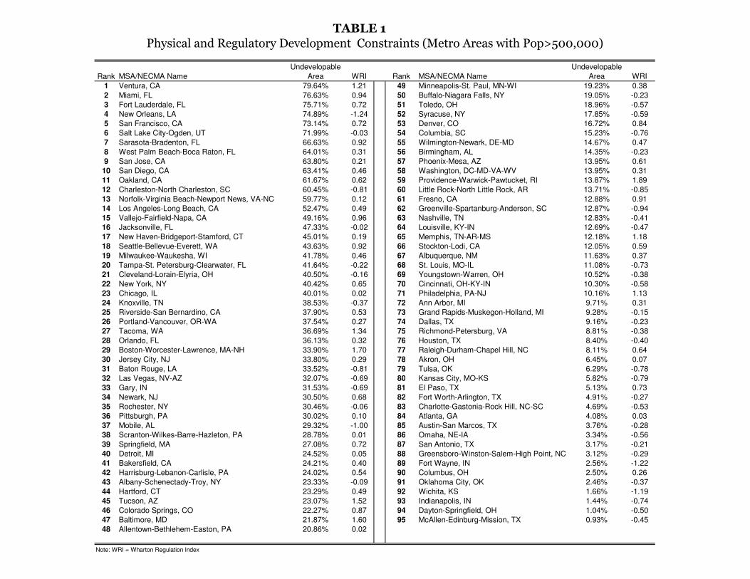
Table 1 displays the percentage of undevelopable area for all metropolitan areas with

population over 500,000 in the 2000 Census for which I also have regulation data (those

included in the later regressions). Of these large metro areas, Ventura (CA) is the most

constrained, with 80 percent of the area within a 50km radius rendered undevelopable by

4

the Pacific Ocean and mountains. Miami, Fort Lauderdale, New Orleans, San Francisco,

Sarasota, Salt Lake City, West Palm Beach, San Diego, and San Jose complete the list of the

top 10 more physically-constrained major metro areas in the US. Many large cities in the

South and Midwest (such as Atlanta, San Antonio, and Columbus) are largely unconstrained.

Table 2 studies the correlates of the newly-constructed land unavailability variable. To

do so, I run a number of independent regressions. The variables in Table 2’s rows appear on

the left-hand-side in each sequential regression, and the geographic-unavailability variable is

always the main right-hand-side control. Regional fixed effects (Northeast, South, Midwest,

West) are included in all regressions. The first column shows the coefficient of the variable of

reference on the unavailable land share, and the second column its associated standard error.

A second set of regressions (2) also controls for a coastal status dummy which identifies

metropolitan areas that are within 100km of the ocean or Great Lakes. The significant

coefficients reveal that geographically land-constrained areas tended to be more expensive in

2000, to have experienced faster price growth since 1970, to have higher incomes, to be more

creative (higher patents per capita), and to have higher leisure amenities (as measured by the

number of tourist visits).3 Observed metropolitan population levels were largely orthogonal

to natural land constraints.

Interestingly, note that none of the major demand-side drivers of recent urban demo-

graphic change (immigration, education, manufacturing orientation, and hours of sun), was

actually correlated with geographic land constraints.

All results hold after controlling for the coastal dummy, indicating that the new land-

availability variable contains information above and beyond that used in studies that focus on

coastal status (Rose, 1989a,b, Malpezzi, 1996). Taking into account the standard deviations

of the different components of land unavailability, mountains contribute towards 42 percent

of the variation in this variable, whereas coastal and internal water loss account for 31 and

26 percent of the variance in land constraints respectively. After controlling for region fixed

effects, as I do throughout the paper, there is no correlation in the data between coastal

area loss and the extent of land constraints begoten by mountainous terrain. The loss of

3Carlino and Saiz (2008) demonstrate that the number of tourism visits is strongly correlated with other

measures of quality of life and a strong predictor of recent city growth.

5

developable land due to the presence of large bodies of internal water (70 percent of which is

attributable to wetlands, as in the Everglades) tends to be positively associated with coastal

area loss and, not surprisingly, negatively associated with mountaineous terrain.

The other major dataset used in the paper is obtained from the 2005 Wharton Regu-

lation Survey. Gyourko, Saiz, and Summers (2008) use the survey to produce a number

of indexes that capture the intensity of local growth control policies in a number of di-

mensions. Lower values in the Wharton Regulation Index, which is standardized across all

municipalities in the original sample, can be thought of as signifying the adoption of more

laissez-faire policies toward real estate development. Metropolitan areas with high values

of the Wharton Regulation Index (WRI henceforth), conversely have zoning regulations or

project approval practices that constrain new residential real estate development. I process

the original municipal-based data to create average regulation indexes by metropolitan area

using the probability sample weights developed by Gyourko, Saiz, and Summers (2008).4

Table 1 displays the average WRI values for all metropolitan areas with populations

greater than 500,000 and for which data is available. A clear pattern arises when contrasting

the regulation index with the land-availability measure. Physical land scarcity is associated

to stricter regulatory constraints to development. 14 out of the top 20 most land-constrained

areas have positive values of the regulation index (which has a mean of -.10 and s.e. of 0.81

across metro areas). Conversely, 16 out of the 20 less land-constrained metropolitan areas

have negative regulation index values.

Other data sources are used throughout the paper: the reader is referred to the Appen-

dixes for descriptive statistics and the meaning and provenance of the remaining variables.

4Note that, because of different sample sizes across cities, in regressions where the WRI is used on the

left-hand side (Table 4) heteroskedasticity could be an issue and therefore Feasible Generalized Least Squares

FGLS are used. In fact, however, the results in Table 4 are very robust to all reasonable weighting schemes

and the omission of metro areas with smaller number of observations in the WRI.

6

3 Geography and Local Development: a Framework

Why should physical or man-made land availability constraints have an impact on housing

supply elasticities? How does geography shape urban development? To characterize the

supply of housing in a city I assume developers to be price takers in the land market.

Consumers within the city compete for locations determining the price of the land input.

Taking land values and construction outlays as given, developers supply housing at cost. All

necesary model derivations and the proofs of propositions are in the mathematical appendix.

The preferences of homogenous consumers in city k are captured by the utility function:

U(Ck) = (Ck)ρ. Consumption in the city (Ck) is the sum of the consumption of city amenities

(Ak) and private goods. Private consumption is equal to wages in the city minus rents, minus

the (monetized) costs of commuting to the CBD, where all jobs are located. Each individual

is also a worker and lives in a separate house, so that the number of housing units equals

population (Hk = POPk). Utility can be thus expressed: U(Ck) = (Ak +wk − γ · r′− t · d)ρ,

where wk stands for the wage in the city, γ for the units of land/housing-space consumption

(assumed constant), r′ for the rent per unit of housing-space consumption, t for the monetary

cost per distance commuted, and d for the distance of the consumer’s residence to the CBD.

As in conventional Alonso-Muth-Mills models (Brueckner, 1987), a non-arbitrage condition

defines the rent gradient: all city inhabitants attain utility Uk via competition in the land

markets. Therefore the total rent paid by an individual (r = γ ·r′) takes the functional form:

r(d) = r0 − td.

Consider a circular city with radius Φk. Geographic or regulatory land constraints make

construction unfeasible in some areas: only a sector (share) Λk of the circle is developable.5

The city radius is thus a function of the number of households and land availability: Φk =√γHkΛk·π

.

Developers are price-takers and buy land at market prices. They build and sell homes

at price P (d). The construction sector is competitive and houses are sold at the cost of

land, LC(d), plus construction costs, CC, which include the profits of the builder: P (d) =

5This feature appears in conventional urban economic models that focus on a representative city (Capozza

and Helesley, 1990). Here, I add heterogeneity in the land availability parameter across cities, and derive

explicit housing supplies elasticities from it.

7

CC+LC(d). In the asset market steady state equilibrium there is no uncertainty and prices

equal the discounted value of rents: P (d) = r(d)i

, which implies r(d) = i ·CC + i ·LC(d). At

the city’s edge there is no alternative use for land so, without loss of generality, LC(Φk) = 0.

Therefore r(Φk) = i · CC, which implies r0 = i · CC + t ·√

γHkΛk·π

.

In this setup, average housing rents in the city, rk, can be shown to be equivalent to

the rents paid by the household living 2/3 of the distance from the CBD to the city’s

edge: rk = r(23Φk)

(see derivation 1 in Mathematical Appendix). The final housing supply

equation in the city has average housing values (P Sk ) expressed as a function of the number

of households:

P Sk = CC +

1

3it ·√

γHk

Λk · π(1)

I next define the aggregate demand function for housing in the city. In a system of

open cities, consumers can move and thus equalize utility across locations, which I normalize

to zero (i.e. the spatial indifference condition is Uk = 0, ∀k) Furthermore, in all cities

and locations wk and Ak are functions of population. I model the level of amenities as:

Ak = Ak − α√POPk. The parameter α mediates the marginal congestion cost (in terms of

rivalry for amenities, traffic, pollution, noise, social capital dilution, crime, etc.). α could also

be interpreted in the context of an alternative but isomorphic model with taste heterogeneity:

people with greater preferences for the city are willing to pay more and move in first, but

later marginal migrants display less of a willingness-to-pay for the city (e.g. Saiz, 2007).

Labor demand is modeled wk = wk − ψ√POPk and is assumed to be downward sloping;

marginal congestion costs weakly increase with population (ψ,α ≥ 0).6 Recalling Hk =

POPk, substituting into the inter-city spatial equilibrium equation, and focusing w.o.l.o.g.

on the spatial indifference condition of consumers living at the CBD I obtain the demand

schedule for housing in the city:

6Of course, cities may display agglomeration economies up to some congestion point (given predetermined

conditions, these may be captured by Ak+ wk). It is only necessary that, in equilibrium, the marginal effect

of population on wages and amenities be (weakly) negative. This is a natural assumption which avoids a

counterfactual equilibria where all activity is concentrated in one single city with AV = 1.

8

√Hk =

Ak + wk

(ψ + α)− i

(ψ + α)P (0) (2)

Note that relative shocks to labor productivity or to amenities (Ak + wk) shift the city’s

demand curve upward, which I will use to identify supply elasticities later.

I can now combine the expression for home values in the CBD via the supply equation

and the city-demand equation (2) to obtain the equilibrium number of households in each

location H∗

k =

(Ak+wk−i·CC

(ψ+α)+t·√

γΛk·π

)2(derivation 2). Note that amenities and wages have to at

least cover the annuitized physical costs of construction for a potential site to be inhabitable.

Within this setup, I first study the supply response to growth in the demand for housing

that is induced by productivity and amenity shocks. Its is clear that ∂PS

k

∂Λk< 0. Other

things equal, more land availability shifts down the supply schedule. Do land constraints

also have an effect with respect to supply elasticities? Defining the city-specific supply

inverse-elasticity of average housing prices as: βSk ≡∂ ln PSk∂ lnHk

one can demonstrate:

Proposition 1

The inverse-elasticity of supply (this is, the price sensitivity to demand shocks) is de-

creasing in land availability. Conversely, as land constraints increase, positive demand shocks

imply stronger positive impacts on the the growth of housing values.

Proposition 1 tells us that land-constrained cities have more inelastic housing supply and

helps us understand how housing prices react to exogenous demand shocks. In addition,

two interesting further questions arise from the general equilibrium in the housing and labor

markets: Why is there any population in areas with difficult housing supply conditions?

Should these areas be more expensive ex-post in equilibrium? Assume that the covariance

between productivity, amenities, and land availability is zero across all locales. Productivity-

amenity shocks are ex-ante independent of physical land availability, which is consistent with

random productivity shocks and Gibrat’s Law explanation for parallel urban growth (Gabaix,

1999). Assume further that the relevant upper tail of such shocks is drawn from a Pareto

distribution. I can now state:

Proposition 2

9

Metropolitan areas with low land availability tend to be more productive or to have

higher amenities; in the observable distribution of metro areas the covariance between land

availability and productivity-amenity shocks in negative.

The intuition for proposition 2 is based on the nature of the urban development process.

As discussed by Eeckhout (2004), existing metropolitan areas are a truncated distribution

of the upper tail of inhabited settlements. In order to compensate for the higher housing

prices that are induced by locations with more difficult supply conditions, consumers need

to be rewarded with higher wages or urban amenities. While costly land development re-

duced ex-ante the desirability of marshlands, wetlands, and mountainous areas for human

habitation, those land-constrained cities that thrived ex post must be more productive or

attractive than comparable locales. Observationally, this implies a positive association be-

tween attractiveness and land constraints, conditional on metropolitan status. Conversely,

land-unconstrained metropolitan areas must be, on average, observationally less productive

and/or amenable.

Note that since the spatial indifference condition has to hold this implies that expected

home values are also decreasing in land availability: metropolitan areas with lower land

availability tend to be more expensive in equilibrium. These conclusions are reinforced if the

ex-ante covariance between productivity/amenities and land availability is negative, albeit

this is not a necessary condition.7

While, due to a selection effect, land-constrained metropolitan areas have higher ameni-

ties, productivity, and prices, they are not necessarily larger. In fact, if productivity-amenity

shocks are approximately distributed Pareto in the upper tail (consistent with the empirical

evidence on the distribution of city sizes in most countries) one can posit:

Proposition 3

Population levels in the existing distribution of metropolitan areas should be independent

of the degree of land availability.

7Glaeser (2005a,b) and Gyourko (2005) emphasize the importance of access to harbors (a factor that

limits land availabilitty) for the earlier development of some of the larger oldest cities in the US: Boston,

New York, and Philadelphia.

10

Proposition 3 tells us that population levels in metropolitan areas are expected to be

orthogonal to initial land availability. In equilibrium higher productivity and/or amenities

are required in more land-constrained cities, which further left-censors their observed distri-

bution of city productivities. With a Pareto distribution of productivity shocks, this effect

exactly compensates for the extra costs imposed by a difficult geography.

In sum, the model tells us that one should expect those geographically-constrained

metropolitan areas that we observe in the data to be more productive or to have higher

amenities (Proposition 2) and the correlation between land availability and population size

to be zero (Proposition 3), precisely the data patterns found in the previous section. In

addition, due to Proposition 3, one should expect metropolitan areas with lower land avail-

ability not only to be more expensive in equilibrium, but also to display lower housing supply

elasticities, as I will demonstrate in the next sections.

4 Geography and Housing Price Elasticities

I now move to assessing how important geographic constraints are to explain local housing

price elasticities. Recall from the model that, on the supply-side, average housing prices in a

city are the sum of construction costs plus land values (themselves a function of the number

of housing units): Pk = CC+LC(Hk). Totally differentiating the log of this expression, and

manipulating, I obtain: d ln Pk =dCC

Pk+ dLC(Hk)

dHk· HkPk· dHkHk

.

For now, I assume changes in local construction costs to be exogenous to local changes

in housing demand: the prices of capital and materials (timber, cement, aluminium, and so

on) are determined at the national or international level, and construction is an extremely

competitive industry with an elastic labor supply. The assumption is consistent with previous

research (Gyourko and Saiz, 2006), but I relax it later. Defining σk =CC

Pkas the initial share

of construction costs on housing prices, and considering that dPkdHk

= dLC(Hk)dHk

, one obtains:

d ln Pk = σk · dCCCC + βSk · dHkHk. As defined earlier in the model, βSk is the inverse-elasticity of

housing supply with respect to average home values. I can re-express this as the empirical

log-linearized supply equation: d ln Pk = σk ·d lnCC+βSk ·d lnHk. Note that by considering

changes in values and quantities initial scale differences across cities are differenced-out

11

(Mayer and Somerville, 2000). Troughout the rest of the paper I use long differences (between

1970 and 2000) and hence focus on long-run housing dynamics, as opposed to high-frequency

volatility.8 However, I will also later briefly discuss results at higher (decadal) frequencies.

The empirical specification also includes region fixed effects (Rjk, for j = 1, 2, 3) and an error

term (εk), and estimates the supply equation in discrete changes:

∆ ln Pk = σk ·∆ lnCCk + βSk ·∆ lnHk +Rjk + εk (3)

Pk is measured by median housing prices in each decennial Census.9 The city-specific

parameter σk (construction cost share in 1970) is calculated using the estimates in Davis and

Heathcote (2007) and Davis and Palumbo (2008), and data on housing prices. Combined

with existing detailed information about the growth of construction costs in each city from

published sources, the city-specific intercept σk·∆ lnCC is thus known and calibrated into the

model. Changes in the housing stock are, of course, endogenous to changes in prices via the

demand-side. Therefore, I instrument for∆ lnHk using a shift-share of the 1974 metropolitan

industrial composition, the log of average hours of sun in January, and the number of new

immigrants (1970 to 2000) divided by population in 1970. The first variable, as introduced

by Bartik (1991) and recently used by Glaeser, Gyourko, Saks (2006), and Saks (2008), is

constructed using early employment levels at the 2-digit SIC level and using national growth

rates in each industry to forecast city-growth due to composition effects. Hours of sun capture

a well-documented secular trend of increasing demand for high-amenity areas (Glaeser et al.

2001; Rappaport, 2007). Finally, previous research (Saiz, 2003, 2007, Ottaviano and Peri,

2007) has shown international migration to be one of the strongest determinants of the

growth in housing demand and prices in a number of major American cities. Immigration

8Short-run housing adjustments involve considerable dynamic aspects, such as lagged construction re-

sponses and serial correlation of high-frequency price changes (Glaeser and Gyourko, 2006).9A long literature, summarized by Kiel and Zabel (1999), demonstrates that the evolution of self-reported

housing prices generally mimics that of actual prices (for a recent confirmation of this fact, see Pence and

Bucks, 2006). The correlation between the change in log median census values and change in the log of the

Freddie Mac repeat sales index between 1980 and 2000 is 0.9 across the 147 cities for which the measures

were available. The repeat sales index, obtained from Freddie Mac, is unavailable in 1970, and its coverage

in our application is limited to the 147 aforementioned cities. Therefore, in this context, I prefer to use the

higher coverage of the Census measure.

12

inflows have been shown to be largely unrelated to other city-wide economic shocks, and very

strongly associated with the pre-determined settlement patterns of immigrant communities

(Altonji and Card, 1989).

The instruments for demand shocks prove to be strong, with an F-test 47.75 compared

to the critical 5 percent value in Stock and Yogo (2005) of 13.91. The instruments also

pass conventional exogeneity tests (with a p-value of 0.6 in the Sargan-Hansen J test). Note

that the specification explicitly controls for all factors that drive physical construction costs.

Equation (3) is estimated using 2SLS, with the assumptions E(εk · Zk) = 0, and with Zk

denoting the exogenous variables: the demand instruments, evolution of construction costs,

the constant, and regional fixed effects in (3).

In Table 3, column 1, I start exploring the data by imposing a common supply inverse-

elasticity parameter for all cities (βSk = βS,∀k). The estimates of βS suggest a relatively

elastic housing supply on average, with an elasticity of 1.54 (1/.65). This is well within the

range of 1 to 3 proposed by the existing literature at the national level (for a review see

Gyourko, 2008). Importantly, unreported regressions where I use each of the demand IV

separately always yield similar and statistically significant results.

From the model in Section 3, I know that the inverse of supply elasticities should be

a function of land availability with ∂βk∂Λk

< 0. A first-degree linear approximation to this

relationship can be posited as: βSk = βS+(1−Λk) ·βLAND.10 The supply equation becomes:

∆ ln Pk = σk ·∆ lnCCk + βS·∆ lnHk + βLAND · (1− Λk) ·∆ lnHk +R

jk + εk (4)

In Table 3, column 2, as in all specifications thereafter, (1 − Λk) - the share of area

unavailable for development - is considered pre-determined and exogenous to supply-side

shocks in the 1970-2000 period. Of course, mountains and coastal status could potentially

be drivers for increased housing demand in the period under consideration. Note, however,

that equation (4) is consistently estimated even if demand shocks ∆ lnHk are also correlated

10Nonlinear versions of the functional relationship between βLANDk and Λk did not add any improvement

of economic or statistical significance to the fit of the supply equation in this small sample of 269 cities. Note

that the specific functional form of ∂βk

∂Λkin the model is driven by the assumptions on the nature of Ricardian

land rents in the model: these are solely due to commuting to the CBD, and commuting costs are linear.

13

with (1 − Λk). Intuitively, land unavailability can be safely included in both the supply

and demand equations insofar there are enough exclusion restrictions specific to the supply

equation.

The results in Table 3, column 2 strongly suggest that the impact of demand on prices

is mediated by physical land unavailability. Moving within the interquartile range of land

unavailability (9 percent to 39 percent), the estimates show the impact of demand shocks on

prices to increase by about 25 percent.

Are the results simply capturing the fact that cities with less land availability tend to

be coastal? Table 3, column 3, allows the impact of demand shocks to vary for coastal and

non-coastal areas. Coastal areas are defined as MSA within 100 kilometers of the ocean (as

calculated by Rappaport and Sachs , 2003). Formally βSk = βS+(1−Λk)·βLAND+COASTk ·

βCOAST , where COAST is a coastal status dummy. The results show the coastal variable to

be not significant. Land unavailability is important within coastal (and non-coastal) areas.

In column 4 of Table 3, the inverse elasticity parameter is approximated by a linear

function of land use regulations and geographic constraints: βSk = βS+ (1− Λk) · βLAND +

lnWRIk · βREG. In this specification lnWRIk stands for the natural log of the Wharton

Regulation Index.11 The supply equation becomes:

∆ ln Pk = σk·∆ lnCCk+βS·∆ lnHk+β

LAND·(1−Λk)·∆lnHk+βREG·lnWRIk·∆ lnHk+R

jk+εk

(5)

For now, lnWRI is assumed to be pre-determined and exogenous to changes in housing

prices through the 1970-2000 period. As in all subsequent specifications hereafter, I cannot

reject that βS= 0: the impact of demand shocks on prices is solely mediated by geographic

and regulatory constraints, which is the assumption that I carry forward. In Table 3, column

5, I explicitly present results of the model with the constraint βS= 0, which largely leaves

the coefficients of interest unchanged.

It is important to remark that independent regressions that consider changes in prices

and housing units in the three decades separately (1970s, 1980s, 1990s) cannot reject the

11I added 3 to the original index to insure that log(WRI) has always positive support, which is consistent

with the theoretical predictions of a positive supply parameter across the board. Alternative (unreported)

normalizations never had major quantitative impacts on the estimates.

14

coefficients on geography and regulations to be statistically equivalent across decades.12

It is apparent that the elasticity of housing supply depends critically on both regulations

and physical constraints. However, standard errors on the land unavailability parameter

are larger. This can be explained by heterogeneity in how binding physical constraints

are. While regulatory constraints matter regardless of the existing level of construction,

physical constraints may not be important until the level of development is large enough to

render them binding Using the model in the previous section, it is straightforward to show

that∂(∂βk∂Λk

)

∂POPk< 0: the (negative) impact of land availability on inverse-elastiticies should

be stronger in larger metro areas. The most parsimonious way to capture this effect is to

model the impact of physical constraints on elasticities as an interacted linear function of

predetermined initial log population levels. In this specification: βSk = (1 − Λk) · βLAND +

(1− Λk) · ln(POPT−1) · βLAND,POP + lnWRI · βREG. Hence the supply equation becomes:

∆ ln Pk =[βLAND + βLAND,POP · ln(POPT−1)

]· (1− Λk) ·∆ lnHk + (6)

σk ·∆lnCCk + βREG · lnWRIk ·∆ lnHk +Rjk + εk

The results in Table 3, column 6, strongly suggest that physical constraints matter more

in larger metropolitan areas, consistent with the theory. Figure 1 depicts the difference

in the inverse of βSk (this is, the supply elasticity) across the interquartile range of land

availability as a function of initial population levels. In the graph, I assign the median level

of regulation to all cities in order to create counterfactuals with respect to differences in

land unavailability exclusively. At the lowest population levels supply elasticity is mostly

determined by regulations: the difference between the 75 percent and 25th percentile in the

distribution of physical land constraints is not large. Nonetheless, geographic constraints

become binding and have a strong impact on prices as metropolitan population becomes

larger. In metropolitan areas above 1,000,000 inhabitants, moving from the 25th to the 75th

percentile of land unavailability implies supply elasticities that are 40 percent smaller.

12The average coefficients across decades are βLAND = 0.29 and βREG = 0.21. Due to the strong mean-

reversion of prices at decadal frequencies, the topography coefficient is closer to zero in the 90s, but larger in

the 80s, whereas the opposite pattern is apparent for the regulation coefficient. They are close to the mean

in the 70s.

15

5 The Indirect Effects of Geography

5.1 Endogenous Regulations

The previous results confirm the well-known empirical link between land use regulations and

housing price growth. Recent examples in this literature include Quigley & Raphael (2005),

Glaeser, Gyourko & Saks (2005a,b), and Saks (2006). However, the existing evidence has

arguably not fully established a causal link: regulations may be endogenous to the evolution

of housing prices.

In the theoretical literature, zoning and growth controls have long been regarded as

endogenous devices to maintain prices high in areas with valuable land (Hamilton, 1975,

Epple, Romer, and Filimon, 1988, Brueckner, 1995). In a review of much of this literature,

Fischel (2001) develops the homevoter hypothesis, according to which zoning and local land

use controls can be largely understood as tools for local homeowners to maximize land prices.

To discuss these issues, consider a stylized version of the supply equation:

∆ ln Pk = β0 + βREG · lnWRIk ·∆ lnHk + β ·∆ lnHk + ξk (7)

Housing supply inverse-elasticities are modelled here as an invariant coefficient (β) plus a

linear function of regulatory constraints (the log of the Wharton Regulation Index). Assume

that, in fact, the local supply elasticity varies for other reasons than regulation that are

uncontrolled for in the model:

∆ ln Pk = β0 + βREG · lnWRIk ·∆ lnHk + β ·∆ lnHk + βδk ·∆ lnHk + ηk︸ ︷︷ ︸ξk

(8)

where βδk is a local deviation from average supply elasticities unrelated to regulation.

Even with suitable instruments for ∆ lnHk, consistent estimates will not be obtained if

lnWRIk is correlated with ξk. Consider as a working hypothesis the following empirical

equation describing the optimal choice of voters with regards to land use policies:

lnWRIk = ϕ0 + ϕ1 · βδk + ϕ2 · βδk ·∆ lnHk + ϕ3 · ln Pk + µk (9)

16

What are the potential sources of regulation endogeneity in equation (9), which includes

an independent error term denoted by µk? In Ortalo-Magné and Prat (2007) voters may

explicitly restrict the supply of land in order to keep its value high, but only have an incentive

to do so in areas where land was initially dear. The only source of supply constraints in

Ortalo-Magné and Prat (2007) comes from regulation, but there are additional reasons why

in areas that were initially land-constrained voters may want further limits on development

(implying ϕ1 > 0 in equation 9). Consider the problem of a voter trying to maximize future

land price growth. From the model in section 2, equilibrium housing prices in an initial steady

state may be obtained as a function of local amenity-productivity levels. Assume now that

we introduce some uncertainty about future amenity-productivity shocks, which are assumed

to be uncorrelated with factors that condition initial population, such as geographic land

availability (Gabaix, 1999). In this context, expected changes to housing prices (E(∆Pk))

are a function of expected productivity shocks (E(∆χk)), as mediated by land availability.

It is staightforward to show (see derivation 3 in the appendix) dE(∆Pk)dΛk

< 0. Reduced

land availability amplifies the effects of productivity shocks on home values. Conversely,

productivity shocks largely translate into population growth in unconstrained cities.

Moreover, d2E(∆Pk)

(dΛk)2 > 0: the marginal impact of additional land constraints on expected

price growth is larger in areas that had already lower land availability initially. The intuition

for this result comes from the geometry of land development. Recall from the model that the

average city radius corresponds to Φk =√

γPOPkΛk·π

; decreasing land availability has a stronger

impact in pushing away the city boundary at low initial values, thereby further increasing

Ricardian land rents. In the presence of positive marginal costs of restrictive zoning, voters

in land-constrained regions have more of an incentive to pass such regulations. Conversely,

marginal changes in zoning regulations do not have much of an expected impact on home

values in areas where land is naturally abundant, thereby reducing their strategic value.

Furthermore, strategic growth-management considerations should be less of an issue in

shrinking cities, where new constraints on growth are not binding, suggesting also that

ϕ2 > 0.

Restrictive land use policies are not exclusively enacted in order to limit the supply of

housing, however. Citizens’ demands for anti-growth regulations partially stem from the

17

perceived nuissances of development, such as increased traffic, school congestion, and aes-

thetic impact on the landscape (Rybczynski, 2007). These issues only arise in growing cities,

and may be more salient in congested areas, where population densities are initially high.

Therefore, restrictive nuisance zoning may be more prevalent in growing, land-constrained

metro areas, which implies again that ϕ2 > 0.

The existing literature offers additional reasons to expect reverse-causality from growing

prices to higher regulations (ϕ3 > 0 in equation 9). Recent examples include Fischel (2001)

and Hilber and Robert-Nicoud (2009), who argue for a demand-side link from higher prices

to increased growth controls. Several mechanisms have been identified that imply such a

reverse causal link.

Rational voters may want to enact restrictive zoning policies in regions with valuable

land even when they do not aim to increase metropolitan housing prices. Changes in the

future local best-and-highest use of land are highly uncertain. Such uncertainty generates

considerable wealth risk on homeowners who are unsure about the nature of future neighbor-

hood change (Breton, 1973). Therefore "since residents cannot insure against neighborhood

change, zoning offers a kind of second-best institution" (Fischel, 2001). In regions with high

land values, voters limit the scope and extent of future land development in their jurisdiction

in order to reduce housing wealth risk. Because all jurisdictions in a region try to deflect risks

and compete à la Tiebout, the equilibrium outcome at the metropolitan level implies stricter

development constraints everywhere. Conversely, concerns about the variability of land val-

ues are absent in regions where home prices are close to, and pinned down by, structural

replacement costs.

Similarly, voters have vested interests in fiscal zoning (Hamilton, 1975, 1976). In areas

with very cheap land, development usually happens at relatively low densities. However, as

land values in a metropolitan area or jurisdiction increase, new entrants into the community

want to consume less land. Simultaneously, in metropolitan areas where the land input is

relatively expensive developers want to use less of it and build at higher densities. However,

existing homeowners do not want new arrivals to pay lower-than-average taxes, which may

induce them to mandate large lot sizes on new development. According to the fiscal-zoning

theories, land use regulations should become more restrictive in areas with expensive land.

18

In order to see if the above theories have empirical content, I start by asking if natural

geographic constraints beget regulatory constraints. Table 4, column 1, displays regressions

similar to equation (9) with the log of the Wharton regulation index on the left-hand side.

The main explanatory variable is the measure of undevelopable area. Geographic constraints

were strongly associated with regulatory constraints in 2005, evidence consistent with ϕ1 > 0

in equation (9). The regression includes other controls, such as regional fixed effects, the

percentage of individuals older than 25 with a bachelor’s degree, and lagged white non-

Hispanic shares.13

Regardless of the evolution of local housing markets, there are regional differences in the

propensity of local governments to regulate economic activity (Kahn, 2002). As a proxy

for preferences for governmental activism (as opposed to laissez-faire) regressions in Table 4

control for the log of the public expenditure on protective inspection and regulation by local

governments at the MSA level as a share of total public revenues. The government expendi-

ture category "Protective inspection and regulation" in the Census of Governments includes

local expenditures in building inspections, weights and measures, regulation of financial in-

stitutions, taxicabs, public service corporations, private utilities; licensing, examination, and

regulation of professional occupations; inspection and regulation or working conditions; mo-

tor vehicle inspection and weighting; and regulation and enforcement of liquor laws and sale

of alcoholic beverages. As expected, areas that tended to regulate economic activity in other

spheres also regulated residential land development more strongly.

Regressions in Table 4 also control for the share of Christians in non-traditional denomi-

nations in 1970, defined as one minus the Catholic and mainline protestant Christian shares.14

Political scientists, economists, and historians of religion have claimed that the ethics and

philosophy of non-traditional Christian denominations (especially those self-denominated

Evangelical) are deeply rooted in individualism and the advocacy for a limited government

13A previous working paper version (Saiz, 2008) explored other potential correlates of land use regulations

across metropolitan areas. Alternative hypotheses based on local politics, optimal regulation of externalities,

and snob-zoning do not change the importance of reverse causation and original land constraints to account

for regulations, and are never quantitatively large.14Mainline Protestant denominations are defined as: United Church, American Baptist, Presbyterian,

Methodist, Lutheran, and Episcopal.

19

role.15 Column 1 in Table 4 (which controls for region fixed effects) finds that a one standard-

deviation increase in the non-traditional Christian share in 1970 was associated with a -0.21

standard-deviation change in land use regulations.

In column 2 of Table 4, I examine another source of endogeneity in equation (9), namely

the possibility that ϕ2 > 0. Land-constrained areas that have been declining or stagnating

for a long time do not seem to display strong anti-growth policies. Consider the case of

Charleston, West Virginia: 71 percent of its 50km radius area is undevelopable according to

our measure, yet the WRI’s value is —1.1. Similar examples are New Orleans (LA), Asheville

(NC), Chattanooga (TN), Elmira (NY), Erie (PA), and Wheeling (WV). In order to capture

the fact that anti-growth regulations may not be important in declining areas, I interact the

geographic-constraints variable by a dummy for MSA in the bottom quartile of urban growth

between 1940 and 1970 (column 2 in Table 4). Lagged growth rates in a period that is, on

average, 45 years in the past, are unlikely to be caused by the regulation environment in

2005. But they are likely to be good predictors of future growth, because of the permanence

of factors that drove productivity during the second half of the 20th century, such as reliance

on manufacturing, mining, or relative scarcity of institutions of higher education. Similarly,

in column 3 of Table 4 I interact the change in housing growth between 1970 and 2000 by

the geographic land-unavailability variable. Of course, housing construction is endogenous

to regulations in this equation. Hence I use the demand shock instruments in Table 3 and

interactions with geographic land unavailability as instrumental variables for the interacted

endogenous variable. The results suggest that regulations are stricter in land-constrained

metro areas that are thriving (ϕ2 > 0). In declining cities, however, regulations are insensitive

to previous factors that made housing supply inelastic.

Finally, in column 4 of Table 4, I test for reverse causation from price levels to higher

regulation (ϕ3 > 0 in equation 9). Since Pt = ∆Pt,t−n + Pt−n, I express the log of housing

values in 2000 as the sum of the change in the log of prices plus the log of initial prices

in 1970 (for comparability with Table 3) and constrain the coefficient on both variables to

15Moberg (1972), Hollinger (1983), Magleby (1992), Holmer-Nadesan (1999), Kyle (2006), Barnett (2008),

Swartz (2008). Crowe (2008) points to a negative correlation between housing price volatility and the Evan-

gelical share, which could be explained by looser land use regulations in Evangelical areas.

20

be the same.16 The instruments now are hours of sun, immigration shocks, and the Bartik

(1991) employment shift-share, and their interactions with geographic land unavailability.

There are 2 endogenous variables: lagged changes in housing prices, and household growth

interacted by the geographic constraints. The equation is estimated via 3SLS, and strongly

suggests that both a constraining geography in growing cities, and higher housing prices led

to a more regulated supply environment circa 2005.

In sum, the regulation equations in Table 4 demonstrate that higher housing prices,

demographic growth, and natural constraints beget more restrictive land-use regulations.

5.2 Endogeneizing Regulations in the Supply Equation

Since regulations are endogenous to εk in equations (5) and (6) one needs to use additional

identifying exclusions to estimate housing supply elasticities. As suggested by the results in

Table 4, the local public expenditure share in protective inspection, and the non-traditional

Christian share in 1970 can be used as instruments for the 2005 WRI: while they predict

land use regulations, they are unlikely to impact land supply otherwise (note that the supply

equation controls for the evolution of construction costs). As seen in Table 4, these variables

prove also to be strong instruments.17 Note that even if these variables were correlated to

demand shocks, the regression have more supply-specific exclusion restrictions than endoge-

nous variables and all parameters are fully identified. In fact, because the two endogenous

variables appear in interacted form, I can now also include to the IV list the interactions of

the instruments used for changes in quantities (hours of sun, employment shift-share, and

immigration shocks) with those used for the regulation index (municipal inspections expen-

diture share and non-traditional Christian share). Importantly, the results are very similar

when I simply use each one of the regulation instruments separately.

Column 1 in Table 5 re-estimates the specification in Table 3, column 5 (elasticities as

linear functions of regulations and geographic constraints), this time allowing for endogenous

16In unconstrained equations, I cannot reject that the separate coefficients on ∆P2000,1970 and P1970 are

statistically equivalent.17Partial R-squared of 0.074 in the first stage and F-test of 10.413, above the 20% maximal bias threshold

(8.75) in Stock and Yogo (2005)

21

regulations. The coefficient on the Wharton Regulation Index declines to about 60 percent of

its previous value. However, when re-estimating the model in equation (6) (land constraints

matter more in large cities), the coefficient on the regulation index takes a value that is

only 8 percent smaller than in the earlier estimates. Therefore, parameters from previous

research are bound to somewhat overestimate the impact of regulations on prices, but it is

still true that more regulated areas tend to be relatively more inelastic, and this impact is

quantitatively large. In Table 5, column 2, a move across the interquartile range in the WRI

of a city of one million inhabitants with average land availability is associated with close to

a 20 percent reduction in supply elasticities: from 1.76 to 1.38.

The impact of constrained geography is larger, especially in larger cities. For example, in

a metro area with average regulations and a population of 1 million, the interquartile change

in the share of unavailable land (from 0.09 to 0.38) implies a 50 percent reduction in supply

elasticities (from 2.45 to 1.25).

In a separate online appendix, the interested reader can further see that endogeneizing

construction costs (which could be themselves a function of geography) and immigration

shocks does not change the main parameters of interest.

5.3 Estimated Elasticities

In this section, I use the coefficients in Table 5, column 2, to estimate supply elasticities

at the metro area level. Such estimates are simple non-linear combinations of the available

data on physical and regulatory constraints, and pre-determined population levels in 2000.

These elasticities are thus based on economic fundamentals related to natural and man-made

land constraints, and should prove useful in calibrating general equilibrium models of inter-

regional labor mobility and to predict the response of housing markets to future demand

shocks.

The population-weighted average elasticity of supply is estimated to be 1.75 in metropol-

itan areas (2.5 unweighted). The results for metropolitan areas with population over 500,000

in 2000 can be found in Table 6. Estimated elasticities using only the geographic, regula-

tory, and initial population variables agree with perceptions about supply-constrained areas.

Miami, Los Angeles, San Francisco, Oakland, New York, San Diego, Boston, Chicago, and

22

Seattle are amongst the top fifteen in the list of most inelastic cities. Houston, Austin, Char-

lotte, Kansas City, and Indianapolis are amongst the large metro areas with highly elastic

housing supply.

Estimated elasticities (this time using pre-determined 1970 population in order to avoid

obvious endogeneity issues) also correlate very strongly with housing price levels in 2000 and

changes over the 1970-2000 period. Figure 2 presents plots relating housing prices (Panel 1)

or changes (Panel 2) on the vertical axis and the inverse of the estimated supply elasticity

by metropolitan area on the horizontal axis. It is clear that a simple linear combination

of physical and regulatory constraints goes very far to explain the evolution of prices, even

without taking into account the differential demand shocks that each city experienced.

6 Conclusion

The paper started by providing empirical content to the concept of land availability in

metropolitan areas. Using satellite-generated data I calculated an exact measure of land

unavailable for real estate development in the metropolitan US. This geographic measure

can be used in future work exploring topics as diverse as housing and mortgage markets,

labor mobility, urban density, transportation, and urban environmental issues.

I then developed a model on the impact of land availability on urban development and

housing prices. In ex-post equilibrium, land-constrained metro areas should have more ex-

pensive housing and enjoy higher amenities or productivity, as confirmed by the data. The

model demonstrates that land constraints should also decrease housing supply elasticities, a

somewhat ad hoc assumption in previous literature.

Empirically, most areas that are widely regarded as supply-inelastic were found, in fact,

to be severely land-constrained by their geography. Deploying a new comprehensive survey

on residential land use regulations, I found that highly-regulated areas tend to also be geo-

graphically constrained. More generally, I found recent housing price and population growth

to be predictive of more restrictive residential land regulations. The results point to the

endogeneity of land use controls with respect to the housing market equilibrium.

Hence I next estimated a model where regulations are both causes and consequences

23

of housing supply inelasticity. Housing demand, construction, and regulations are all de-

termined endogenously. Housing supply elasticities were found to be well-characterized as

functions of both physical and regulatory land constraints, which in turn are endogenous to

prices and past growth.

Geography was shown to be one of the most important determinants of housing supply

inelasticity: directly, via reductions in the amount of land availability, and indirectly, via

increased land values and higher incentives for anti-growth regulations. The results in the

paper demonstrate that geography is a key factor in the contemporaneous urban development

of the United States, and help us understand why robust national demographic growth and

increased urbanization has translated mostly into higher housing prices in San Diego, New

York, Boston, and LA, but into rapidly growing populations in Atlanta, Phoenix, Houston,

and Charlotte.

24

References

[1] Alonso, W. Location and land use, Cambridge, Mass.: Harvard University Press (1964).

[2] Altonji, Joseph & David Card, (1989). "The Effects of Immigration on the Labor Market

Outcome of Less-Skilled Natives," Working Papers 636, Princeton University, Department

of Economics, Industrial Relations Section..

[3] Barnett, Timothy (2008). “Evangelicals and Economic Enlightment.” Paper for the 2008

Annual Conference of The American Political Science Association

[4] Bartik, T. (1991). “Who benefits from state and local economic development policies?”

W.E. Upjohn Institute for Employment Research, Kalamazoo, MI.

[5] Breton, A. (1973). “Neighborhood Selection and Zoning.” In Issues in Urban Public

Economics, ed. Harold Hochman. Saarbrucken: institute Internationale de Finance

Publique.

[6] Brueckner, J, (1987). “The Structure of Urban Equilibria: A Unified Treatment of the

Muth-Mills Model.” In E.S. Mills (Ed.): Handbook of Regional and Urban Economics,

Volume II, Elsevier.

[7] Brueckner, J.K. (1995). “Strategic control of growth in a system of cities.” Journal of

Public Economics, vol. 57, No. 3, pp. 393-416.

[8] Bucks, B. and K. Pence (2006). “Do Homeowners Know Their House Values and Mortgage

Terms?” FEDS Working Paper No. 2006-03.

[9] Burchfield, M, Overman H.G., Puga, D. and M.A. Turner (2006). “Causes of sprawl: A

portrait from space” Quarterly Journal of Economics, 121(2), May 2006: 587-633

[10] Capozza, Dennis R. & Helsley, Robert W., (1990) "The stochastic city," Journal of Urban

Economics, Elsevier, vol. 28(2), pages 187-203, September.

[11] Carlino, J, and A. Saiz (2008). “Beautiful City: Leisure Amenities and Urban Growth.”

Working Paper SSRN-1280157.

[12] Combes, P.P., Duranton, G., Gobillon, L. and S. Roux (2009). “Estimating Agglomeration

Economies with History, Geology, and Worker Effects.” Working Paper.

[13] Crowe, C. (2009). “Irrational Exuberance in the U.S. Housing market: Were Evangelicals

Left Behind?” IMF Working Paper 09/57.

[14] Davis, M. and J. Heathcote (2007). “The Price and Quantity of Residential Land in the

United States.” Journal of Monetary Economics, vol. 54, No. 8, pp. 2595-2620.

[15] Davis, M. and M.G. Palumbo (2008). “The Price of Residential Land in Large U.S.

Cities,” Journal of Urban Economics, vol. 63, No. 1, pp. 352-384.

[16] Eckout, J. (2004) “Gibrat’s Law for (All) Cities”, American Economic Review 94(5), 2004,

1429-1451

[17] Epple, D., T. Romer, and R. Filimon (1988). “Community Development with Endogenous

Land Use Controls.” Journal of Public Economics, vol. 35, pp. 133-162.

[18] Fischel, W. (1985). The Economics of Zoning Laws: A Property Rights Approach to

American Land Use Controls. Baltimore: Johns Hopkins University Press.

[19] Fischel, W. (2001). The Homevoter Hypothesis: How Home Values Influence Local

Government. Cambridge, Mass.: Harvard University Press.

[20] Gabaix, X. (1999). “Zipf's Law For Cities: An Explanation.” Quarterly Journal of

Economics, Vol. 114, No. 3, Pages 739-767

[21] Glaeser, Edward (2005a). “Urban Colossus: Why New York is America’s Largest City,”

Federal Reserve Bank of New York Economic Policy Review 11(2), 2005: 7-24.

[22] Glaeser, Edward (2005b) “Reinventing Boston: 1640-2003 ”Journal of Economic

Geography 5(2), 119-153

[23] Glaeser, E. and J. Gyourko (2003). “The Impact of Building Restrictions on Housing

Affordability.” Federal Reserve Bank of New York’s Economic Policy Review, pp. 21-39.

[24] Glaeser, E. and J. Gyourko (2006). “Housing Cycles.” NBER working paper 12787

[25] Glaeser, E., J. Gyourko and R. Saks (2005a). “Why Is Manhattan So Expensive?

Regulation and Rise in Housing Prices.” Journal of Law and Economics, vol. 48, No. 2, pp.

331-370.

[26] Glaeser, E., J. Gyourko and R. Saks (2005b). “Why Have Housing Prices Gone Up?”,

American Economic Review, vol. 95. No. 2, pp. 329-333.

[27] Glaeser, E., J. Gyourko, and R. Saks (2006). “Urban Growth and Housing Supply.”

Journal of Economic Geography, vol. 6, No. 1, pp. 71–89.

[28] Glaeser, Edward L., Jed Kolko, and Albert Saiz, (2001) "Consumer city," Journal of

Economic Geography, Oxford University Press, vol. 1(1), pages 27-50

[29] Glaeser, E. and A. Saiz (2004). “The Rise of the Skilled City.” Brookings-Wharton Papers

on Urban Affairs, 2004. The Brookings Institution: Washington D.C.

[30] Gyourko, Joseph (2005). “Looking Back to Look Forward: What Can We Learn About

Urban Development from Philadelphia’s 350-Year History?”, Brookings-Wharton Papers

on Urban Affairs, forthcoming.

[31] Gyourko, Joseph (2008). “Housing Supply.” Working Paper, Zell-Lurie Real Estate

Center: The Wharton School: university of Pennsylvania.

[32] Gyourko, J. and A. Saiz (2006). “Construction Costs and the Supply of Housing

Structure.” Journal of Regional Science, vol. 46, No. 4, pp. 661-680.

[33] Gyourko, J., A. Saiz and A.A. Summers (2008). “A New Measure of the Local Regulatory

Environment for Housing Markets: The Wharton Residential Land Use Regulatory Index.”

Urban Studies, vol. 45, No. 3, pp. 693-729.

[34] Hamilton, Bruce W. (1975). “Zoning and Property Taxation in a System of Local

Governments.” Urban Studies 12 (June): pp.205-211

[35] Hamilton, Bruce W. (1976). “Capitalization of Intrajurisdictional Differences in Local Tax

Prices.” American Economic Review 99(Dec): pp.743-753

[36] Hilber, C. and F. Robert-Nicaud (2006). “Owners of Developed Land Versus Owners of

Undeveloped Land: Why Land Use is More Constrained in the Bay Area than in

Pittsburgh.” CEP Discussion Paper No 760 (LSE).

[37] Hollinger (1983). “Individualism and Social Ethics: an Evangelical Syncretism.” University

Press of America: Boston.

[38] Holmer Nadesan, Majia (1999). The discourses of corporate spiritualism and evangelical

capitalism. Management Communication Quarterly : McQ, 13(1), 3-42.

[39] Hwang, M. and J. Quigley (2004). “Economic Fundamentals in Local Housing Markets:

Evidence from U.S. Metropolitan Regions.” Journal of Regional Science, vol. 46, No. 3, pp.

425-453.

[40] Katz, L. and K.T. Rosen (1987). "The Interjurisdictional Effects of Growth Controls on

Housing Prices." Journal of Law and Economics, vol. 30, No. 1, pp. 149-60.

[41] Kahn, M. (2002). “Demographic Change and the Demand for Environmental Regulation.”

Journal of Policy Analysis and Management, vol. 21, No. 1, pp. 45-62.

[42] Kiel, Katherine A. and Jeffrey E. Zabel (1999) "The Accuracy of Owner-Provided House

Values: The 1978-1991 American Housing Survey," Real Estate Economics, vol. 27(2),

pages 263-298.

[43] Kyle Richard G. (2006) ”Evangelicalism: An Americanized Christianity” Transaction

Publishers

[44] Magleby, D. B. 1992. Political behavior. In The encyclopedia of Mormonism, edited by D.

Ludlow. New York: Macmillan.

[45] Malpezzi, S., G.H. Chun, and R.K. Green (1998). “New Place-to-Place Housing Price

Indexes for U.S. Metropolitan Areas, and Their Determinants.” Real Estate Economics,

vol. 26, No. 2, pp. 235-274.

[46] Malpezzi, S. (1996). “Housing Prices, Externalities, and Regulation in U.S. Metropolitan

Areas.” Journal of Housing Research, vol. 7, No. 2, pp. 209-41.

[47] Mayer, C.J. and C.T. Somerville (2000). “Residential Construction: Using the Urban

Growth Model to Estimate Housing Supply.” Journal of Urban Economics, vol. 48, pp. 85-

109.

[48] Mills, E. (1967). “An aggregative model of resource allocation in a metropolitan area.”

American Economic Review, vol. 57, No. 2, pp. 197-210.

[49] Moberg David O. (1972) “The Great Reversal: Evangelism and Social Concern”,

Philadelphia, J. B. Lippincott & Co.

[50] Muth, R., (1969), “Cities and housing,” Chicago: University of Chicago Press.

[51] Ortalo-Magne, F. and A. Prat (2007). "The Political Economy of Housing Supply:

Homeowners, Workers, and Voters." LSE: STICERD - Theoretical Economics Paper Series

No. /2007/514.

[52] Ottavianno, G. and G. Peri (2007). "The Effects of Immigration on US Wages and Rents:

A General Equilibrium Approach." CEPR Discussion Papers 6551 (revised).

[53] Pence, K.M. and B. Bucks (2006). "Do Homeowners Know Their House Values and

Mortgage Terms? " FEDS Working Paper No. 2006-03.

[54] Quigley, J.M. and S. Raphael (2005). “Regulation and the High Cost of Housing in

California.” American Economic Review, vol. 94, No. 2, pp. 323-328.

[55] Rappaport, Jordan, (2007) "Moving to nice weather," Regional Science and Urban

Economics, Elsevier, vol. 37(3), pages 375-398

[56] Rappaport, J. and J.D. Sachs (2003). "The United States as a Coastal Nation." Journal of

Economic Growth 8, 1 (March), pp. 5--46.

[57] Rose, L.A. (1989a). “Topographical Constraints and Urban Land Supply Indexes.” Journal

of Urban Economics, vol. 26, No. 3, pp. 335-347.

[58] Rose, L.A. (1989b). “Urban Land Supply: Natural and Contrived Reactions.” Journal of

Urban Economics, vol. 25, pp. 325-345.

[59] Rybczynski, Witold (2007). “Last Harvest: How a Cornfield became New Daleville.”

Scribner: New York.

[60] Saiz, A. (2003). "Room in the Kitchen for the Melting Pot: Immigration and Rental

Prices." The Review of Economics and Statistics, vol. 85, No. 3, pp. 502-521

[61] Saiz, A. (2007). "Immigration and housing rents in American cities." Journal of Urban

Economics, vol. 61, No. 2, pp. 345-371.

[62] Saiz, A. (2008). “On Local Housing Supply Elasticity” Working Paper: SSRN#1193422.

[63] Saks, R. (2008). “Job Creation and Housing Construction: Constraints on Metropolitan

Area Employment Growth.” Journal of Urban Economics, 64(1), pp.178-195.

[64] Stock, J. H., and M. Yogo. (2005). “Testing for weak instruments in linear IV

regression.” In Identification and Inference for Econometric Models: Essays in Honor of

Thomas Rothenberg, ed. D. W. K. Andrews and J. H. Stock, 80-108. Cambridge:

Cambridge University Press.

[65] Rosenthal, S. and W.C Strange, (2008)."The attenuation of human capital spillovers,"

Journal of Urban Economics, vol. 64(2), pages 373-389, September.

[66] Swartz, David R. (2008) “Left Behind: The Evangelical Left and the Limits of Evangelical

Politics: 1965-1988.” Ph.D. Dissertation (History) University of Notre Dame.

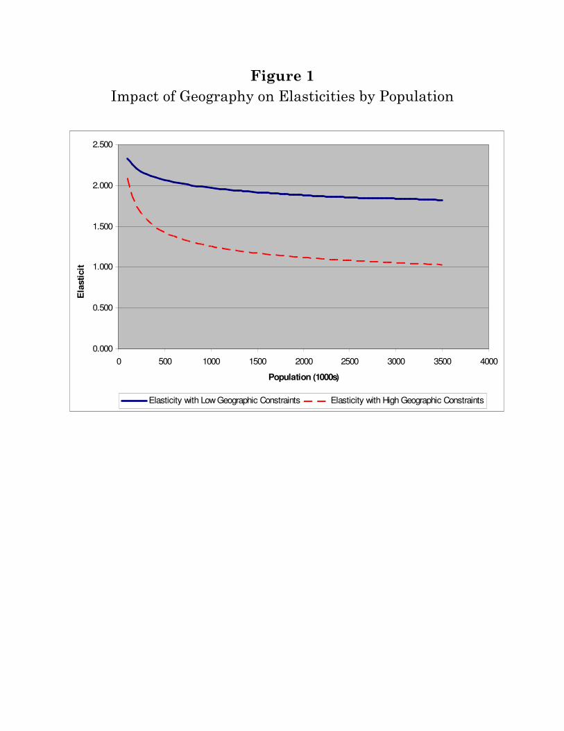
Figure 1

Impact of Geography on Elasticities by Population

0.000

0.500

1.000

1.500

2.000

2.500

0 500 1000 1500 2000 2500 3000 3500 4000

Population (1000s)

Ela

sti

cit

y

Elasticity with Low Geographic Constraints Elasticity with High Geographic Constraints

Figure 2: Estimated Elasticities and Home Values (2000) 2.1: Levels

2.2: Changes

11

11.5

12

12.5

13

0 .5 1 1.5 2 Inverse of Supply Elasticity

Log median house value Fitted values

1.5

2

2.5

3

0 .5 1 1.5 2 Inverse of Supply Elasticity

Log Price 2000 - Log Price 1970 Fitted values

Rank MSA/NECMA Name

Undevelopable

Area WRI Rank MSA/NECMA Name

Undevelopable

Area WRI

1 Ventura, CA 79.64% 1.21 49 Minneapolis-St. Paul, MN-WI 19.23% 0.38

2 Miami, FL 76.63% 0.94 50 Buffalo-Niagara Falls, NY 19.05% -0.23

3 Fort Lauderdale, FL 75.71% 0.72 51 Toledo, OH 18.96% -0.57

4 New Orleans, LA 74.89% -1.24 52 Syracuse, NY 17.85% -0.59

5 San Francisco, CA 73.14% 0.72 53 Denver, CO 16.72% 0.84

6 Salt Lake City-Ogden, UT 71.99% -0.03 54 Columbia, SC 15.23% -0.76

7 Sarasota-Bradenton, FL 66.63% 0.92 55 Wilmington-Newark, DE-MD 14.67% 0.47

8 West Palm Beach-Boca Raton, FL 64.01% 0.31 56 Birmingham, AL 14.35% -0.23

9 San Jose, CA 63.80% 0.21 57 Phoenix-Mesa, AZ 13.95% 0.61

10 San Diego, CA 63.41% 0.46 58 Washington, DC-MD-VA-WV 13.95% 0.31

11 Oakland, CA 61.67% 0.62 59 Providence-Warwick-Pawtucket, RI 13.87% 1.89

12 Charleston-North Charleston, SC 60.45% -0.81 60 Little Rock-North Little Rock, AR 13.71% -0.85

13 Norfolk-Virginia Beach-Newport News, VA-NC 59.77% 0.12 61 Fresno, CA 12.88% 0.91

14 Los Angeles-Long Beach, CA 52.47% 0.49 62 Greenville-Spartanburg-Anderson, SC 12.87% -0.94

15 Vallejo-Fairfield-Napa, CA 49.16% 0.96 63 Nashville, TN 12.83% -0.41

16 Jacksonville, FL 47.33% -0.02 64 Louisville, KY-IN 12.69% -0.47

17 New Haven-Bridgeport-Stamford, CT 45.01% 0.19 65 Memphis, TN-AR-MS 12.18% 1.18

18 Seattle-Bellevue-Everett, WA 43.63% 0.92 66 Stockton-Lodi, CA 12.05% 0.59

19 Milwaukee-Waukesha, WI 41.78% 0.46 67 Albuquerque, NM 11.63% 0.37

20 Tampa-St. Petersburg-Clearwater, FL 41.64% -0.22 68 St. Louis, MO-IL 11.08% -0.73

21 Cleveland-Lorain-Elyria, OH 40.50% -0.16 69 Youngstown-Warren, OH 10.52% -0.38

22 New York, NY 40.42% 0.65 70 Cincinnati, OH-KY-IN 10.30% -0.58

23 Chicago, IL 40.01% 0.02 71 Philadelphia, PA-NJ 10.16% 1.13

24 Knoxville, TN 38.53% -0.37 72 Ann Arbor, MI 9.71% 0.31

25 Riverside-San Bernardino, CA 37.90% 0.53 73 Grand Rapids-Muskegon-Holland, MI 9.28% -0.15

26 Portland-Vancouver, OR-WA 37.54% 0.27 74 Dallas, TX 9.16% -0.23

27 Tacoma, WA 36.69% 1.34 75 Richmond-Petersburg, VA 8.81% -0.38

28 Orlando, FL 36.13% 0.32 76 Houston, TX 8.40% -0.40

29 Boston-Worcester-Lawrence, MA-NH 33.90% 1.70 77 Raleigh-Durham-Chapel Hill, NC 8.11% 0.64

30 Jersey City, NJ 33.80% 0.29 78 Akron, OH 6.45% 0.07

31 Baton Rouge, LA 33.52% -0.81 79 Tulsa, OK 6.29% -0.78

32 Las Vegas, NV-AZ 32.07% -0.69 80 Kansas City, MO-KS 5.82% -0.79

33 Gary, IN 31.53% -0.69 81 El Paso, TX 5.13% 0.73

34 Newark, NJ 30.50% 0.68 82 Fort Worth-Arlington, TX 4.91% -0.27

35 Rochester, NY 30.46% -0.06 83 Charlotte-Gastonia-Rock Hill, NC-SC 4.69% -0.53

36 Pittsburgh, PA 30.02% 0.10 84 Atlanta, GA 4.08% 0.03

37 Mobile, AL 29.32% -1.00 85 Austin-San Marcos, TX 3.76% -0.28

38 Scranton-Wilkes-Barre-Hazleton, PA 28.78% 0.01 86 Omaha, NE-IA 3.34% -0.56

39 Springfield, MA 27.08% 0.72 87 San Antonio, TX 3.17% -0.21

40 Detroit, MI 24.52% 0.05 88 Greensboro-Winston-Salem-High Point, NC 3.12% -0.29

41 Bakersfield, CA 24.21% 0.40 89 Fort Wayne, IN 2.56% -1.22

42 Harrisburg-Lebanon-Carlisle, PA 24.02% 0.54 90 Columbus, OH 2.50% 0.26

43 Albany-Schenectady-Troy, NY 23.33% -0.09 91 Oklahoma City, OK 2.46% -0.37

44 Hartford, CT 23.29% 0.49 92 Wichita, KS 1.66% -1.19

45 Tucson, AZ 23.07% 1.52 93 Indianapolis, IN 1.44% -0.74

46 Colorado Springs, CO 22.27% 0.87 94 Dayton-Springfield, OH 1.04% -0.50

47 Baltimore, MD 21.87% 1.60 95 McAllen-Edinburg-Mission, TX 0.93% -0.45

48 Allentown-Bethlehem-Easton, PA 20.86% 0.02

TABLE 1

Physical and Regulatory Development Constraints (Metro Areas with Pop>500,000)

Note: WRI = Wharton Regulation Index

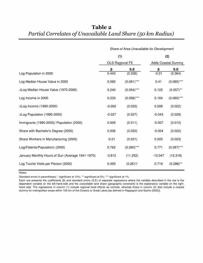
β S.E β S.E

Log Population in 2000 0.443 (0.336) -0.01 (0.364)

Log Median House Value in 2000 0.592 (0.081)*** 0.41 (0.085)***

∆Log Median House Value (1970-2000) 0.240 (0.054)*** 0.122 (0.057)**

Log Income in 2000 0.233 (0.056)*** 0.164 (0.060)***

∆Log Income (1990-2000) -0.002 (0.020) 0.006 (0.022)

∆Log Population (1990-2000) -0.027 (0.027) -0.043 (0.029)

Immigrants (1990-2000)/ Population (2000) 0.009 (0.011) -0.007 (0.012)

Share with Bachelor's Degree (2000) 0.006 (0.020) -0.004 (0.022)

Share Workers in Manufacturing (2000) -0.01 (0.021) 0.005 (0.023)

Log(Patents/Population) (2000) 0.762 (0.260)*** 0.771 (0.287)***

January Monthly Hours of Sun (Average 1941-1970) -3.812 (11.252) -12.047 (12.318)

Log Tourist Visits per Person (2000) 0.493 (0.261)* 0.719 (0.286)**

Notes:

Standard errors in parentheses; * significant at 10%; ** significant at 5%; *** significant at 1%

Each row presents the coefficients (β) and standard errors (S.E) of separate regressions where the variable described in the row is the

dependent variable on the left-hand-side and the unavailable land share (geographic constraint) is the explanatory variable on the right-

hand side. The regressions in column (1) include regional fixed effects as controls, whereas those in column (2) also include a coastal

dummy for metropolitan areas within 100 km of the Oceans or Great Lakes [as defined in Rappaport and Sachs (2003)].

Table 2

OLS-Regional FE Adds Coastal Dummy

Partial Correlates of Unavailable Land Share (50 km Radius)

(1) (2)

Share of Area Unavailable for Development

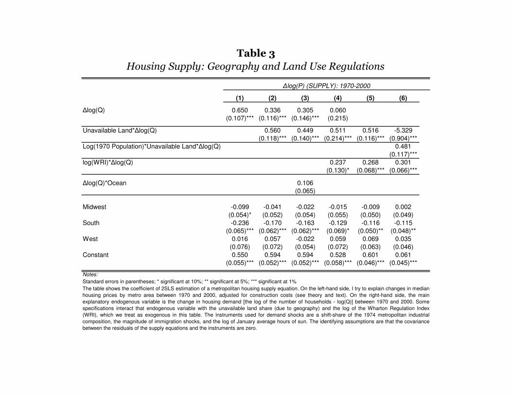
(1) (2) (3) (4) (5) (6)

∆log(Q) 0.650 0.336 0.305 0.060

(0.107)*** (0.116)*** (0.146)*** (0.215)

Unavailable Land*∆log(Q) 0.560 0.449 0.511 0.516 -5.329

(0.118)*** (0.140)*** (0.214)*** (0.116)*** (0.904)***

Log(1970 Population)*Unavailable Land*∆log(Q) 0.481

(0.117)***

log(WRI)*∆log(Q) 0.237 0.268 0.301

(0.130)* (0.068)*** (0.066)***

∆log(Q)*Ocean 0.106

(0.065)

Midwest -0.099 -0.041 -0.022 -0.015 -0.009 0.002

(0.054)* (0.052) (0.054) (0.055) (0.050) (0.049)

South -0.236 -0.170 -0.163 -0.129 -0.116 -0.115

(0.065)*** (0.062)*** (0.062)*** (0.069)* (0.050)** (0.048)**

West 0.016 0.057 -0.022 0.059 0.069 0.035

(0.076) (0.072) (0.054) (0.072) (0.063) (0.046)

Constant 0.550 0.594 0.594 0.528 0.601 0.061

(0.055)*** (0.052)*** (0.052)*** (0.058)*** (0.046)*** (0.045)***

Notes:

Standard errors in parentheses; * significant at 10%; ** significant at 5%; *** significant at 1%

∆log(P) (SUPPLY): 1970-2000

Housing Supply: Geography and Land Use Regulations

Table 3

The table shows the coefficient of 2SLS estimation of a metropolitan housing supply equation. On the left-hand side, I try to explain changes in median

housing prices by metro area between 1970 and 2000, adjusted for construction costs (see theory and text). On the right-hand side, the main

explanatory endogenous variable is the change in housing demand [the log of the number of households - log(Q)] between 1970 and 2000. Some

specifications interact that endogenous variable with the unavailable land share (due to geography) and the log of the Wharton Regulation Index

(WRI), which we treat as exogenous in this table. The instruments used for demand shocks are a shift-share of the 1974 metropolitan industrial

composition, the magnitude of immigration shocks, and the log of January average hours of sun. The identifying assumptions are that the covariance

between the residuals of the supply equations and the instruments are zero.

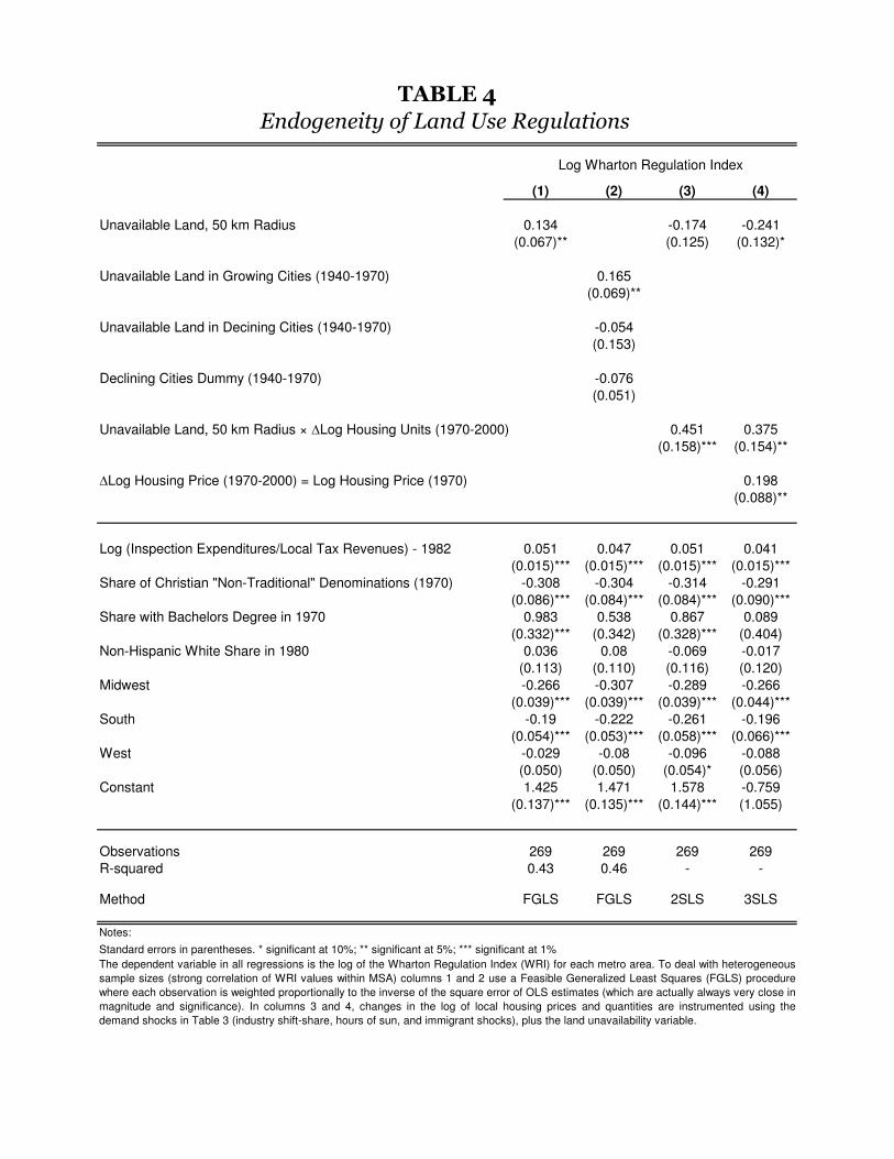
(1) (2) (3) (4)

Unavailable Land, 50 km Radius 0.134 -0.174 -0.241

(0.067)** (0.125) (0.132)*

Unavailable Land in Growing Cities (1940-1970) 0.165

(0.069)**

Unavailable Land in Decining Cities (1940-1970) -0.054

(0.153)

Declining Cities Dummy (1940-1970) -0.076

(0.051)

Unavailable Land, 50 km Radius × ∆Log Housing Units (1970-2000) 0.451 0.375

(0.158)*** (0.154)**

∆Log Housing Price (1970-2000) = Log Housing Price (1970) 0.198

(0.088)**

Log (Inspection Expenditures/Local Tax Revenues) - 1982 0.051 0.047 0.051 0.041

(0.015)*** (0.015)*** (0.015)*** (0.015)***

Share of Christian "Non-Traditional" Denominations (1970) -0.308 -0.304 -0.314 -0.291

(0.086)*** (0.084)*** (0.084)*** (0.090)***

Share with Bachelors Degree in 1970 0.983 0.538 0.867 0.089

(0.332)*** (0.342) (0.328)*** (0.404)

Non-Hispanic White Share in 1980 0.036 0.08 -0.069 -0.017

(0.113) (0.110) (0.116) (0.120)

Midwest -0.266 -0.307 -0.289 -0.266

(0.039)*** (0.039)*** (0.039)*** (0.044)***

South -0.19 -0.222 -0.261 -0.196

(0.054)*** (0.053)*** (0.058)*** (0.066)***

West -0.029 -0.08 -0.096 -0.088

(0.050) (0.050) (0.054)* (0.056)

Constant 1.425 1.471 1.578 -0.759

(0.137)*** (0.135)*** (0.144)*** (1.055)

Observations 269 269 269 269

R-squared 0.43 0.46 - -

Method FGLS FGLS 2SLS 3SLS

Notes:

Standard errors in parentheses. * significant at 10%; ** significant at 5%; *** significant at 1%

Log Wharton Regulation Index

TABLE 4

Endogeneity of Land Use Regulations

The dependent variable in all regressions is the log of the Wharton Regulation Index (WRI) for each metro area. To deal with heterogeneous

sample sizes (strong correlation of WRI values within MSA) columns 1 and 2 use a Feasible Generalized Least Squares (FGLS) procedure

where each observation is weighted proportionally to the inverse of the square error of OLS estimates (which are actually always very close in

magnitude and significance). In columns 3 and 4, changes in the log of local housing prices and quantities are instrumented using the

demand shocks in Table 3 (industry shift-share, hours of sun, and immigrant shocks), plus the land unavailability variable.

(1) (2)

Unavailable Land*∆log(Q) 0.581 -5.260

(0.119)*** (1.396)***

Log(1970 Population)*Unavailable Land*∆log(Q) 0.475

(0.119)***

log(WRI)*∆log(Q) 0.109 0.280

(0.078)* (0.077)***

Midwest -0.009 0.002

(0.049) (0.048)

South -0.075 -0.109

(0.049) (0.049)**

West 0.149 0.059

(0.063) (0.065)

Constant 0.659 0.577

(0.048)*** (0.048)***

Notes:

The table shows the coefficient of 2SLS estimation of a metropolitan housing supply equation. The

specification and instruments used for demand shocks are as in Table 3. Demand shocks are

interacted with the unavailable land share (due to geography) and the log of the Wharton Regulation

Index. The latter variable is treated as endogenous using the share of local public expenditures on

"protective inspections" and the share of non-traditional Christian denominations as instruments. Since

we are instrumenting for log(WRI)*∆log(Q) I also include the interaction between the regulation and

the demand instruments in the IV list.

Housing Supply: Endogenous Regulations

Table 5

Standard errors in parentheses; * significant at 10%; ** significant at 5%; *** significant at 1%

∆log(P) (SUPPLY)

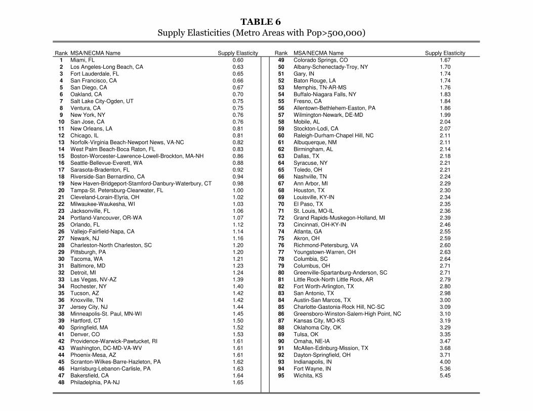
Rank MSA/NECMA Name Supply Elasticity Rank MSA/NECMA Name Supply Elasticity

1 Miami, FL 0.60 49 Colorado Springs, CO 1.67

2 Los Angeles-Long Beach, CA 0.63 50 Albany-Schenectady-Troy, NY 1.70

3 Fort Lauderdale, FL 0.65 51 Gary, IN 1.74

4 San Francisco, CA 0.66 52 Baton Rouge, LA 1.74

5 San Diego, CA 0.67 53 Memphis, TN-AR-MS 1.76

6 Oakland, CA 0.70 54 Buffalo-Niagara Falls, NY 1.83

7 Salt Lake City-Ogden, UT 0.75 55 Fresno, CA 1.84

8 Ventura, CA 0.75 56 Allentown-Bethlehem-Easton, PA 1.86

9 New York, NY 0.76 57 Wilmington-Newark, DE-MD 1.99

10 San Jose, CA 0.76 58 Mobile, AL 2.04

11 New Orleans, LA 0.81 59 Stockton-Lodi, CA 2.07

12 Chicago, IL 0.81 60 Raleigh-Durham-Chapel Hill, NC 2.11

13 Norfolk-Virginia Beach-Newport News, VA-NC 0.82 61 Albuquerque, NM 2.11

14 West Palm Beach-Boca Raton, FL 0.83 62 Birmingham, AL 2.14

15 Boston-Worcester-Lawrence-Lowell-Brockton, MA-NH 0.86 63 Dallas, TX 2.18

16 Seattle-Bellevue-Everett, WA 0.88 64 Syracuse, NY 2.21

17 Sarasota-Bradenton, FL 0.92 65 Toledo, OH 2.21

18 Riverside-San Bernardino, CA 0.94 66 Nashville, TN 2.24

19 New Haven-Bridgeport-Stamford-Danbury-Waterbury, CT 0.98 67 Ann Arbor, MI 2.29

20 Tampa-St. Petersburg-Clearwater, FL 1.00 68 Houston, TX 2.30

21 Cleveland-Lorain-Elyria, OH 1.02 69 Louisville, KY-IN 2.34

22 Milwaukee-Waukesha, WI 1.03 70 El Paso, TX 2.35

23 Jacksonville, FL 1.06 71 St. Louis, MO-IL 2.36

24 Portland-Vancouver, OR-WA 1.07 72 Grand Rapids-Muskegon-Holland, MI 2.39

25 Orlando, FL 1.12 73 Cincinnati, OH-KY-IN 2.46

26 Vallejo-Fairfield-Napa, CA 1.14 74 Atlanta, GA 2.55

27 Newark, NJ 1.16 75 Akron, OH 2.59

28 Charleston-North Charleston, SC 1.20 76 Richmond-Petersburg, VA 2.60

29 Pittsburgh, PA 1.20 77 Youngstown-Warren, OH 2.63

30 Tacoma, WA 1.21 78 Columbia, SC 2.64

31 Baltimore, MD 1.23 79 Columbus, OH 2.71

32 Detroit, MI 1.24 80 Greenville-Spartanburg-Anderson, SC 2.71

33 Las Vegas, NV-AZ 1.39 81 Little Rock-North Little Rock, AR 2.79

34 Rochester, NY 1.40 82 Fort Worth-Arlington, TX 2.80

35 Tucson, AZ 1.42 83 San Antonio, TX 2.98

36 Knoxville, TN 1.42 84 Austin-San Marcos, TX 3.00

37 Jersey City, NJ 1.44 85 Charlotte-Gastonia-Rock Hill, NC-SC 3.09

38 Minneapolis-St. Paul, MN-WI 1.45 86 Greensboro-Winston-Salem-High Point, NC 3.10

39 Hartford, CT 1.50 87 Kansas City, MO-KS 3.19

40 Springfield, MA 1.52 88 Oklahoma City, OK 3.29

41 Denver, CO 1.53 89 Tulsa, OK 3.35

42 Providence-Warwick-Pawtucket, RI 1.61 90 Omaha, NE-IA 3.47

43 Washington, DC-MD-VA-WV 1.61 91 McAllen-Edinburg-Mission, TX 3.68

44 Phoenix-Mesa, AZ 1.61 92 Dayton-Springfield, OH 3.71

45 Scranton-Wilkes-Barre-Hazleton, PA 1.62 93 Indianapolis, IN 4.00

46 Harrisburg-Lebanon-Carlisle, PA 1.63 94 Fort Wayne, IN 5.36

47 Bakersfield, CA 1.64 95 Wichita, KS 5.45

48 Philadelphia, PA-NJ 1.65

TABLE 6

Supply Elasticities (Metro Areas with Pop>500,000)

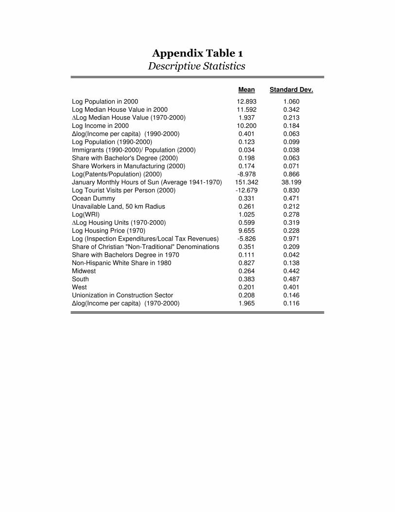
Mean Standard Dev.

Log Population in 2000 12.893 1.060

Log Median House Value in 2000 11.592 0.342

∆Log Median House Value (1970-2000) 1.937 0.213

Log Income in 2000 10.200 0.184

∆log(Income per capita) (1990-2000) 0.401 0.063

Log Population (1990-2000) 0.123 0.099

Immigrants (1990-2000)/ Population (2000) 0.034 0.038

Share with Bachelor's Degree (2000) 0.198 0.063

Share Workers in Manufacturing (2000) 0.174 0.071

Log(Patents/Population) (2000) -8.978 0.866

January Monthly Hours of Sun (Average 1941-1970) 151.342 38.199

Log Tourist Visits per Person (2000) -12.679 0.830

Ocean Dummy 0.331 0.471

Unavailable Land, 50 km Radius 0.261 0.212

Log(WRI) 1.025 0.278

∆Log Housing Units (1970-2000) 0.599 0.319

Log Housing Price (1970) 9.655 0.228

Log (Inspection Expenditures/Local Tax Revenues) -5.826 0.971

Share of Christian "Non-Traditional" Denominations 0.351 0.209

Share with Bachelors Degree in 1970 0.111 0.042

Non-Hispanic White Share in 1980 0.827 0.138

Midwest 0.264 0.442

South 0.383 0.487

West 0.201 0.401

Unionization in Construction Sector 0.208 0.146

∆log(Income per capita) (1970-2000) 1.965 0.116

Appendix Table 1

Descriptive Statistics

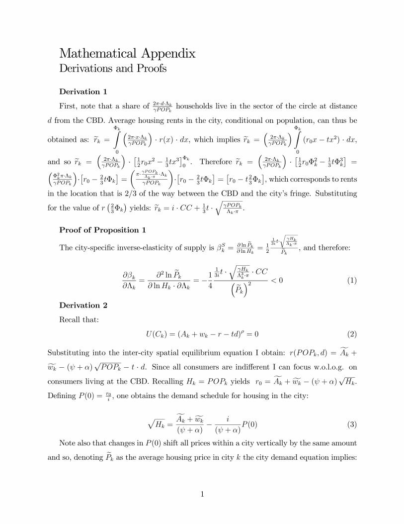
Mathematical AppendixDerivations and Proofs

Derivation 1

First, note that a share of 2π·d·ΛkγPOPk

households live in the sector of the circle at distance

d from the CBD. Average housing rents in the city, conditional on population, can thus be

obtained as: rk =

Φk∫

0

(2π·x·ΛkγPOPk

)· r(x) · dx, which implies rk =

(2π·ΛkγPOPk

) Φk∫

0

(r0x− tx2) · dx,

and so rk =(2π·ΛkγPOPk

)·[12r0x

2 − 13tx3]Φk0. Therefore rk =

(2π·ΛkγPOPk

)·[12r0Φ

2k −

13tΦ3k]=

(Φ2kπ·Λk

γPOPk

)·[r0 − 2

3tΦk]=

(π· γPOPk

Λk·π·Λk

γPOPk

)·[r0 − 2

3tΦk]=[r0 − t23Φk

], which corresponds to rents

in the location that is 2/3 of the way between the CBD and the city’s fringe. Substituting

for the value of r(23Φk)yields: rk = i · CC + 1

3t ·√

γPOPkΛk·π

.

Proof of Proposition 1

The city-specific inverse-elasticity of supply is βSk =∂ ln Pk∂ lnHk

= 12

13it·√

γHkΛk·π

Pk, and therefore:

∂βk∂Λk

=∂2 ln Pk

∂ lnHk · ∂Λk= −

1

4

13it ·√

γHkΛ3k·π · CC

(Pk

)2 < 0 (1)

Derivation 2

Recall that:

U(Ck) = (Ak + wk − r − td)ρ = 0 (2)

Substituting into the inter-city spatial equilibrium equation I obtain: r(POPk, d) = Ak +

wk − (ψ + α)√POPk − t · d. Since all consumers are indifferent I can focus w.o.l.o.g. on

consumers living at the CBD. Recalling Hk = POPk yields r0 = Ak + wk − (ψ + α)√Hk.

Defining P (0) = r0i, one obtains the demand schedule for housing in the city:

√Hk =

Ak + wk(ψ + α)

−i

(ψ + α)P (0) (3)

Note also that changes in P (0) shift all prices within a city vertically by the same amount

and so, denoting Pk as the average housing price in city k the city demand equation implies:

1

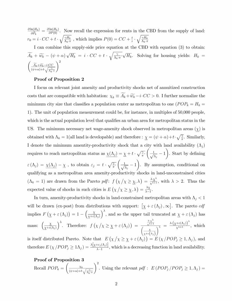
∂ ln(Hk)

∂Pk= ∂ ln(Hk)

∂P (0). Now recall the expression for rents in the CBD from the supply of land:

r0 = i · CC + t ·√

γHkΛk·π

, which implies P (0) = CC + ti·√

γHkΛk·π

I can combine this supply-side price equation at the CBD with equation (3) to obtain:

Ak + wk − (ψ + α)√Hk = i · CC + t ·

√γ

Λk·π·√Hk. Solving for housing yields: Hk =

(Ak+wk−i·CC(ψ+α)+t·

√γ

Λk·π

)2

Proof of Proposition 2

I focus on relevant joint amenity and productivity shocks net of annuitized construction

costs that are compatible with habitation: χk ≡ Ak+wk−i ·CC > 0. I further normalize the

minimum city size that classifies a population center as metropolitan to one (POPk = Hk =

1). The unit of population measurement could be, for instance, in multiples of 50,000 people,

which is the actual population level that qualifies an urban area for metropolitan status in the

US. The minimum necessary net wage-amenity shock observed in metropolitan areas (χ) is

obtained with Λk = 1(all land is developable) and therefore : χ = (ψ + α)+t ·√

γ

π. Similarly,

I denote the minimum amentity-productivity shock that a city with land availability (Λj)

requires to reach metropolitan status as χ(Λj) = χ + t ·√

γ

π·(

1√Λj− 1). Start by defining

ε (Λj) = χ(Λj) − χ , to obtain εj = t ·√

γ

π·(

1√Λj− 1). By assumption, conditional on

qualifying as a metropolitan area amenity-productivity shocks in land-unconstrained cities

(Λk = 1) are drawn from the Pareto pdf : f(χ/χ ≥ χ, λ

)=

λ·χλ

χλ+1, with λ > 2. Thus the

expected value of shocks in such cities is E(χ/χ ≥ χ, λ

)=

λχ

λ−1 .

In turn, amenity-productivity shocks in land-constrained metropolitan areas with Λj < 1

will be drawn (ex-post) from distributions with support:[χ+ ε (Λj) ,∞

]. The pareto cdf

implies F(χ+ ε (Λj)

)= 1 −

(χ

χ+ε(Λj)

)λ, and so the upper tail truncated at χ + ε (Λj) has

mass:(

χ

χ+ε(Λj)

)λ. Therefore: f

(χ/χ ≥ χ+ ε (Λj)

)=

λ·χλ

χλ+1(χ

χ+ε(Λj)

)λ =λ·(χ+ε(Λj))

λ

χλ+1, which

is itself distributed Pareto. Note that E(χ/χ ≥ χ + ε (Λj)

)= E (χ /POPj ≥ 1,Λj ), and

therefore E (χ /POPj ≥ 1Λj ) =λ[χ+εj(Λj)]

λ−1 , which is a decreasing function in land availability.

Proof of Proposition 3

Recall POPk =

(χk

(ψ+α)+t·√

γΛk ·π

)2. Using the relevant pdf : E (POPj /POPj ≥ 1,Λj ) =

2

∞∫

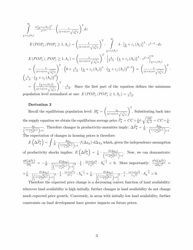
χ+εj(Λj)

λ·[χ+εj(Λj)]λ

zλ+1·(

z

(ψ+α)+t·√

γΛk ·π

)2dz

E (POPj /POPj ≥ 1,Λj ) =(

1

(ψ+α)+t·√

γΛk ·π

)2·

∞∫

χ+εj(Λj)

λ ·[χ+ εj (Λj)

]λ · z1−λ · dz

E (POPj /, POPj ≥ 1,Λj ) =(

1

(ψ+α)+t·√

γΛk·π

)2·[

λ2−λ ·

(χ+ εj (Λj)

)λ · z2−λ]∞χ+εj(Λj)

=

(1

(ψ+α)+t·√

γΛk·π

)2·(0 + λ

λ−2 ·(χ+ εj (Λj)

)λ ·(χ+ εj (Λj)

)2−λ)=

(1

(ψ+α)+t·√

γΛk·π

)2·

(λλ−2 ·

(χ + εj (Λj)

)2)

=

((χ+εj(Λj))

(ψ+α)+t·√

γΛk·π

)2· λλ−2 . Since the first part of the equation defines the minimum

population level normalized at one: E (POPj /POPj ≥ 1,Λj ) = λλ−2 .

Derivation 3

Recall the equilibrium population level: H∗k =

(χk

(ψ+α)+t·√

γΛk·π

)2. Substituting back into

the supply equation we obtain the equilibrium average price P ∗k = CC+13it·√

γH∗k

Λk·π= CC+ 1

3i·

χk(ψ+α

√Λk·π

t·√γ

)+1. Therefore changes in productivity-amenities imply: ∆P ∗k =

13i· ∆χk(

ψ+α√Λk·π

t·√γ

)+1.

The expectation of changes in housing prices is therefore:

E(∆P ∗k

)=

∫13i· ∆χk(

ψ+α√Λk·π

t·√γ

)+1·f(∆χk)·d∆χk which, given the independence assumption

of productivity shocks implies: E(∆P ∗k

)= 1

3i· E(∆χk)(

ψ+α√Λk·π

t·√γ

)+1. Now, we can demonstrate:

dE(∆P ∗k )dΛk

= − 13i· E(∆χk)[(

ψ+α√Λk·π

t·√γ

)+1

]2 · 12 ·(ψ+α)

√π

t·√γ · Λ−1

2

k < 0. More importantly:d2E(∆P ∗k )(dΛk)

2 =

+ 13i· E(∆χk)[(

ψ+α√Λk·π

t·√γ

)+1

]3 · 12 ·(ψ+α)2πt2·γ · Λ−

1

2

k + 13i· E(∆χk)[(

ψ+α√Λk·π

t·√γ

)+1

]2 · 14· (ψ+α)

√π

t·√γ · Λ−3

2

k > 0.

Therefore the expected price change is a decreasing convex function of land availability:

wherever land availability is high initially, further changes in land availability do not change

much expected price growth. Conversely, in areas with initially low land availability, further

constraints on land development have greater impacts on future prices.

3

Data Appendix

1. Data sources

Variable Source Notes

Land Unavailability Calculated by author from

elevation and land use GIS

data from USGS

Wharton Regulation Index Gyourko, Saiz, Summers (2007) See Data section in text

Declining Metro Area: 1950-

1970

Calculated by author from data

in Historical Census Browser –

University of Virginia

A dummy that takes value 1 if

growth is in the lowest quartile of the

metro areas in our sample.

Non-Hispanic White Share

(1970)

HUD State of the Cities

Database (from Census)

BA/BS share (1970) HUD State of the Cities

Database (from Census)

Foreign-Born Share (1970) HUD State of the Cities

Database (from Census)

Tourist Visits per Person (2000) Saiz and Carlino (2008)

Log Patents per Capita Glaeser and Saiz (2004)

Immigration Shock HUD State of the Cities

Database (from Census)

The difference in the number of

foreign-born individuals between

1970 and 2000, divided by metro area

population in 1970

Share workers in manufacturing

1970

HUD State of the Cities

Database (from Census)

Median Housing price

(1970,2000)

HUD State of the Cities

Database (from Census)

Number of Hosing Units

(1970,2000)

HUD State of the Cities

Database (from Census)

Percentage of Christians in

“Non-Traditional”

Churches and Church

membership in the United

Calculated as one minus the share of

Catholic Church adherents and

denominations, 1971 States, 1971 – The Association

of Religion data Archives

mainline protestants (United Church,

American Baptist, Presbyterian,

Methodist, Lutheran, and Episcopal).

% Voting for Carter (1980) County and City data Book

1983

Local Tax Revenues in 1982 Census of Governments 1982 2000 county-based metropolitan

definitions were used to aggregate at

the metro level.

Inspection Expenditures/Local

Tax Revenues 1982

Census of Governments 1982

Coastal Metro Area Dummy Rappaport and Saks (2003) A dummy that takes value one if the

minimum distance in an MSA’s

county is below 100 km.

January Monthly Hours of Sun

(Average 1941-1970)

Natural Amenities Scale –

USDA Economic Research

Service

Construction Costs (Single

Family, Average Quality)

Gyourko and Saiz (2006) –

Originally from Means and Co.

Housing Price Repeat Sales

Index

Freddie Mac purchase-only

Conventional Mortgage Home

Price Index

Land value shares Davis and Heathcote (2006)

Davis and Palumbo (2008)

Davis and Heathcote (2006)

calculate the average share of land

for residential real estate in the US in

1970 to be 20%. In 1984 (the first

year for which their metropolitan

data series is available), Davis and

Palumbo (2008) suggest national and

metropolitan land shares to be very

similar. We therefore adapt an

unweighted average 20% land share

across metropolitan areas in 1970..

We then calculate differences in the

structure cost/value ratio by dividing

the average construction cost in 1970

for a 2,000 sq. ft. home (the average

home size) by the median home value

in each metro area. The final

metropolitan-level estimate of

structural shares in 1970 ( 1itα −

) is

proportional to the aforementioned

ratio, and such that its unweighted

mean across metro areas is 80%.

Central City Areas 1970, 2000 County and City Data Books

1972, 2002