The genomic impacts of drift and selection for hybrid performance in maize

Justin P. Gerke*1, Jode W. Edwards§, Katherine E. Guill†, Jeffrey Ross-Ibarra‡ and Michael D.

McMullen*†

*Division of Plant Sciences, University of Missouri, Columbia MO 65211

§Corn Insects and Crop Genetics Research Unit, USDA-Agricultural Research Service, Ames,

IA, 50011

†Plant Genetics Research Unit, USDA-Agricultural Research Service, Columbia MO 65211

‡Department of Plant Sciences, Center for Population Biology, and Genome Center, University

of California, Davis, CA 95616

1 Present address: DuPont Pioneer, Johnston, Iowa

Running Title: Drift and selection in maize improvement

Key Words / Phrases: Recurrent selection; heterosis; genetic drift; population structure; high-throughput genotyping

Corresponding Author:Justin P. GerkeDuPont Pioneer8305 NW 62ND AveP.O. Box 7060Johnston, IA, 50131justin.gerke@gmail.com

ABSTRACT

Modern maize breeding relies upon selection in inbreeding populations to improve the

performance of cross-population hybrids. The United States Department of Agriculture -

Agricultural Research Service (USDA-ARS) reciprocal recurrent selection experiment between

the Iowa Stiff Stalk Synthetic (BSSS) and the Iowa Corn Borer Synthetic No. 1 (BSCB1)

populations represents one of the longest standing models of selection for hybrid performance.

To investigate the genomic impact of this selection program, we used the Illumina MaizeSNP50

high-density SNP array to determine genotypes of progenitor lines and over 600 individuals

across multiple cycles of selection. Consistent with previous research (Messmer et al., 1991;

Labate et al., 1997; Hagdorn et al., 2003; Hinze et al., 2005), we found that genetic diversity

within each population steadily decreases, with a corresponding increase in population structure.

High marker density also enabled the first view of haplotype ancestry, fixation and

recombination within this historic maize experiment. Extensive regions of haplotype fixation

within each population are visible in the pericentromeric regions, where large blocks trace back

to single founder inbreds. Simulation attributes most of the observed reduction in genetic

diversity to genetic drift. Signatures of selection were difficult to observe in the background of

this strong genetic drift, but heterozygosity in each population has fallen more than expected.

Regions of haplotype fixation represent the most likely targets of selection, but as observed in

other germplasm selected for hybrid performance (Feng et al., 2006), there is no overlap between

the most likely targets of selection in the two populations. We discuss how this pattern is likely to

occur during selection for hybrid performance, and how it poses challenges for dissecting the

impacts of modern breeding and selection on the maize genome.

INTRODUCTION

Although maize is naturally an out-crossing organism, modern breeding develops highly

inbred lines that are then used in controlled crosses to produce hybrids. Hybrid maize has been

so successful that it quickly replaced long-standing mass-selected open pollinated varieties

(Crabb, 1947). Maize inbred lines are now partitioned into separate inbreeding ‘heterotic groups’

that maximize performance and hybrid vigor (heterosis) when an inbred line of one group is

crossed with the other group (Tracy and Chandler, 2006). The shift towards selection of inbred

lines based on their ability to generate good hybrids – referred to as ‘combining ability’ –

constituted an abrupt change from the open-pollinated mass selection that breeders practiced for

millennia (Anderson, 1944; Troyer, 1999).

Multiple studies with molecular markers have indicated that the modern era of single-

cross hybrid maize breeding has led to a dramatic restructuring of population genetic variation

(Duvick et al., 2004; Ho et al., 2005; Feng et al., 2006). Different heterotic groups have diverged

genetically over time to become highly structured and isolated populations. Advances in high

throughput genotyping and the development of a maize reference genome now enable the

observation of maize population structure at high marker density across the whole genome

(Ganal et al., 2011; Chia et al., 2012). So far, these high-density studies have examined a broad

spectrum of germplasm at various points in the history of maize to search for the signals of

population structure and artificial selection (Hufford et al., 2012; van Heerwaarden et al., 2012).

Although selective sweeps remaining from domestication are clearly visible, the impact of

selection during modern breeding appears comparatively small in terms of its impact on genomic

diversity despite steady, heritable improvement in phenotype (Duvick, 2005). The lack of distinct

selection signals from modern breeding may be due to specific selective events occurring in

different populations, necessitating a more focused look within heterotic groups or even single

breeding programs.

In this study, we apply a genomic approach to study the dynamics of genetic variation

over time within an individual selection experiment. The Iowa Stiff Stalk Synthetic (BSSS) and

the Iowa Corn Borer Synthetic No. 1 (BSCB1) Reciprocal Recurrent Selection Program of the

USDA-ARS at Ames, Iowa (hereafter referred to as the Iowa RRS) represents one of the best-

documented public experiments on selection for combining ability and hybrid performance.

BSSS and BSCB1 have been recurrently selected for improved cross-population hybrids (Penny

and Eberhart, 1971). This model of selection, named reciprocal recurrent selection, provides the

generalized model for strategies used in commercial maize breeding (Comstock et al., 1949;

Duvick et al., 2004). The Iowa RRS experiment proves especially relevant because lines derived

from the BSSS population have had a major impact upon the development of commercial

hybrids (Duvick et al., 2004; Darrah and Zuber, 1986), the formation of modern heterotic groups

(Troyer, 1999; Senior et al., 1998), and the choice of a maize reference genome (Schnable et al.,

2009).

MATERIALS AND METHODS

The BSSS and BSCB1 Recurrent Selection Program: The Iowa RRS experiment began with

founder inbred lines (Table S1) that were randomly mated to create the BSSS and BSCB1 ‘cycle

0’ base populations. Each group was then recurrently selected for improved combining ability

with the other group (Penny and Eberhart, 1971; Keeratinijakal and Lamkey, 1993). Initially

approximately 200-250 starting ‘S0’ plants within each population were simultaneously self-

fertilized to generate ‘S1’ lines and crossed to a random sample (4-6) of plants from the other

population to generate testcross seed. The material was evaluated for highly heritable traits

including standability, disease resistance and ear rot resistance in the nursery at the time the

testcross seed was made, and 100 testcrosses were then grown in replicated field trials and

evaluated for grain yield, grain moisture, and standability. S1 seed of 10 selected families within

each population were randomly mated to create a new ‘cycle n+1’ population. After cycle 4, the

testcrosses were carried out on the S1 lines themselves rather than at S0, which leads to another

round of selfing prior to the creation of the next cycle. Ten lines (out of 100) were selected and

advanced to form the next cycle between cycles 1 and 8, and twenty lines were selected between

cycles 9 and 16 (Keeratinijakal and Lamkey, 1993). Founder inbreds and samples from cycles 0,

4, 8, 12, and 16 were genotyped at 39,258 SNPs that passed a set of quality filters and could be

assigned collinear genetic and physical map positions.

Plants and inbred lines used: The plants and inbred lines used in this experiment are

listed in Table S1. We genotyped 36 plants from each of the BSSS and BSCB1 populations at

selection cycles 0, 4, 8, 12, and 16. These plants represent descendants of the original

populations which have been randomly mated to maintain seed. We also genotyped the founder

inbreds for each population, however, seed for the founder lines F1B1, CI.617, WD456, and

K230 were not available. The data for founder line CI.540 was not used because the genotyped

material was heterozygous. A number of derived lines were also genotyped for calibrating

phasing and imputation procedures (see below).

Genotype data: Plants from the cycles of selection, founders, and derived lines were

grown in a greenhouse and tissue was collected at the 3 leaf stage. Tissue was lyophilized,

ground, and DNA extracted by a CTAB procedure (Saghai-Maroof et al., 1984). Samples were

genotyped using the 24-sample Illumina MaizeSNP50 array (Ganal et al., 2011) according to the

Illumina Infinium protocol, and imaged on an Illumina BeadStation at the University of Missouri

DNA core facility. Genotypes were determined with the GenomeStudio v2010.2 software using

the MaizeSNP50_B.egt cluster file, (http://www.illumina.com/support/downloads.ilmn). The

design of the maize SNP50 Chip included a relatively small ascertainment panel of inbred lines,

introducing a bias in the frequencies of SNPs included on the chip (Ganal et al., 2011). However,

because our simulations are based not on theoretical expectations but instead on sampling from

the observed data at cycle 0, we expect ascertainment bias to have a minimal impact on our

results. The effect of this ascertainment bias was shown to be minimal in another study of North

American germplasm (van Heerwaarden et al., 2012).

48,919 SNPs were called on the Illumina platform from the MaizeSNP50_B.egt cluster

file. Genotypes with quality scores of 50 or less were recoded as missing data. Three plants were

removed from the data due to an excess of missing data (the derived line B10, a cycle 0 plant

from BSSS, and a cycle 8 plant from BSSS). In addition, BSCB1 plant 31 from cycle 4 appeared

switched with plant 31 from cycle 8 based on our principal component analysis (PCA), so we

switched the labels for these two genotypes to correct the mistake. To avoid structure among the

missing data, we removed any SNP that was coded as missing in more than 3 plants in either

group of founders or any group of plants from a particular cycle and population. Preliminary

analysis by PCA and heatmap plots of distance matrices revealed two additional likely mix-ups.

Plant 23 from BSSS cycle 8 was a clear outlier from the BSSS population as a whole and plant 2

from BSSS cycle 0 is likely a mislabeled plant from cycle 16. Since there was no evidence

suggesting when mis-labelings occurred, each of these plants was removed from the analysis.

Integrating the genetic and physical map: The interpretation of our results depends

upon a genetic and physical map that is as accurate as possible. We therefore took steps to

improve the positions of the SNP markers on the genetic and physical maps relative to version

5A.59 of the maize genome assembly (maizesequence.org). The probable physical position of

each SNP based was obtained by comparing SNP context sequences to the genome sequence. For

this purpose, SNP context sequences were defined as the sequence 25 bp upstream of the SNP,

the bp representing the SNP itself, followed by 25 bp downstream of the SNP, making a total

sequence length of 51bp. When a single genomic location was queried by two separate probes on

the array, we chose the probe with higher quality calls and dropped the other marker from the

dataset.

To assign a genetic position for each SNP, we used a map derived from the B73xMo17

(IBM) mapping population similar to the IBM framework map in Ganal et al. (Ganal et al.,

2011). This genetic map contains 4,217 framework SNP markers, which provides a much higher

density than the map used to order the 5A.59 release of the maize genome sequence. As a result,

we identified several places in the genome where the physical positions were incorrect according

to our genetic map. These cases included both simple reversals of the physical map relative to the

genetic map, and also the assignment of blocks of markers to the wrong linkage group, which we

refer to as mis-mapped blocks. SNPs at these loci were reordered to match our genetic map. To

maintain collinearity between the genetic and physical map, the physical positions of these SNPs

were reassigned as follows. Individual mis-mapped markers were simply removed from the data.

We also removed small reversals and mis-mapped blocks (<10 kb). Small rearrangements of this

sort are more likely to represent mis-mapped paralagous sequence than true errors in the physical

map. When larger reversals were identified, we transposed the physical positions of the SNPs

from one end of the segment to the other. Mis-mapped blocks were often larger than the physical

gap into which they were moved. We therefore assigned the first SNP of the block to a position

10 kb downstream from the previous SNP on the correct linkage group. We then recalculated

genomic coordinates for the rest of the chromosome based on the marker distances within the

translocated segment. The last SNP of the block was also given a 10 kb cushion between itself

and the next SNP on the correct linkage group.

Only a portion of the SNPs on the array had genetically mapped positions. ‘Unmapped’

SNPs (those with a physical position but no genetic position) bounded by two mapped markers

were moved along with their mapped neighbors if both anchoring mapped markers were also

moved. However, it is unclear whether unmapped SNPs just outside of these anchors should be

kept in place or moved along with the adjacent SNPs. Since most inversions were small relative

to the genetic map (and would therefore still fall in the same window of a sliding window

analysis), these SNPs were left in place. However, markers bordering translocations were

removed to ensure there were no markers mapped to the incorrect linkage group. Unmapped

SNPs were then assigned a genetic position by linear interpolation of genetic vs. physical

distance using the approx() function in R (www.R-project.org). The IBM genetic map distances

were then converted to single-meiosis map distances using the formulae of Winkler et al.

(Winkler et al., 2003). Finally, SNPs located at physical positions outside of those bounded by

the genetic map (such as the telomeres) were assigned the genetic position of their nearest

mapped neighbor. Since moved segments were arbitrarily joined 10 kb from their nearest genetic

neighbor, we acknowledge that the physical positions of these markers are only estimates.

However, the estimated junctions are small relative to the genetic windows used for our analysis.

The final map used is provided as supplemental material (Supplementary File S1)

Haplotype phasing: Although the genotypes of the plants from each population are

unphased, the homozygous genotypes of the founders and derived inbreds provide excellent prior

information for a probabilistic estimation of genotype phase in the populations. We therefore

used fastPHASE (Scheet and Stephens, 2006) to estimate the genotype phase of each plant. To

estimate the error in phasing, we created test cases by combining the genotypes of two derived

inbreds into a hypothetical “F1 hybrid” of unknown phase. This F1 was presented to fastPHASE

with the rest of the data, except that its parent inbreds were removed. Analyses of several

hypothetical F1’s from different cycles of selection revealed very low phasing error rates (Table

S3). Therefore the phased genotypes of cycle 0 plants were used as the starting data for

simulations (see below).

Diversity and principal component analysis: Heterozygosity (H) was measured as:

H = 2p(1-p)

where p and (1-p) are the frequencies of the two SNP alleles. FST (Hudson et al., 1992)was

calculated using the HBKpermute program in the analysis package of the software library

libsequence (Thornton, 2003). All results were plotted using the R package ggplot2 (Wickham,

2009). We conducted PCA by singular value decomposition, as described in (McVean, 2009).

Simulations: Our simulation sought to model the effects of genetic drift in the Iowa

RRS experiment independent of any selection, and our model thus closely followed the

published methods of the Iowa RRS (Penny and Eberhart, 1971; Keeratinijakal and Lamkey,

1993). Starting individuals in each population were constructed by randomly sampling two

distinct haplotypes with replacement from the phased haplotypes of cycle 0. In the actual random

mating scheme used in the Iowa RRS experiment, a single pairing could only contribute four

gametes to the next generation (two kernels each from two ears), and our simulation reflects this.

Advanced cycles were simulated by randomly mating gametes from self-fertilized plants of the

previous cycle until 10 new individuals were created. The first cycle involved two rounds of

random mating, whereas all subsequent cycles used one round. After cycle 5, the process

employed two rounds of selfing instead of one. After cycle 7, the population size was increased

from 10 to 20. At cycles 4, 8, 12, and 16, the plants were randomly mated to match the sample

size of the observed data. The genotypes of these simulated random matings are the final results

of each simulation that were analyzed in the same way as the observed data.

All recombination events in the simulations were carried out in R with the hypred

software package (cran.r-project.org/web/packages/hypred/). The simulations were executed in

parallel on a computing cluster, with unique random number seeds drawn for each simulation.

Statistics were calculated for each simulation using the same formula as with the experimental

data. We used non-overlapping sliding windows of equal genetic distance to account for the non-

independence of markers in low-recombination regions when calculating measures of

significance. For the haplotype-based, single-locus simulations, recombination was simply

replaced with binomial sampling of two alleles.

RESULTS

Increase in population structure and loss of genetic diversity: Founder inbreds and

samples from cycles 0, 4, 8, 12, and 16 were genotyped at 39,258 SNPs that passed a set of

quality filters and could be assigned collinear genetic and physical map positions (See Materials

and Methods for details). Change in population structure throughout the Iowa RRS experiment

can be observed visually by a principal component analysis (PCA). A joint analysis of

individuals from all the selection cycles (Figure 1) clearly separates the BSSS and BSCB1

populations along the first axis of variation, with increasing separation as the experiment

progressed. The second axis of variation primarily separates the cycles from one another within

each population. There is no separation between the founders of the two populations, but at cycle

0, the BSSS population shows more divergence from the founders than does BSCB1. This could

be due to drift during either the population’s construction or its subsequent maintenance.

Structure continued to develop within each population over the course of the experiment. There

is an especially wide gap between cycles 4 and 8, which correlates with the addition of an extra

generation of self-pollination prior to selection at each cycle. The distance between cycles then

decreases dramatically after cycle 8, and this corresponds to doubling in effective population

size.

No new genetic material was intentionally introduced into either population after the

experiments’ inception, so the substantial increase in genetic distance could only arise from the

loss of genetic diversity within each population. Consistent with previous studies of the Iowa

RRS, genome-wide genetic diversity decreased steadily across cycles of selection in both

populations (Figure 2). The decrease in heterozygosity (H) was much smaller when the two

populations are combined, indicating the loss of different alleles within BSCB1 and BSSS. This

leads to strong genetic differentiation, as FST rose by a factor of ten between the founder lines and

the populations at cycle 16.

We noticed an irregular increase in the number of polymorphic markers between BSSS

cycles 4 and 8 (Table S2). All of these newly polymorphic markers were present at extremely

low frequency and were spread among various individuals. This may represent a series of minor

alleles that were not captured in our sample of cycle 4 individuals and thus appeared to

‘resurface’ at cycle 8. Alternatively, the pattern may be the result of minor contamination at some

point in the population’s history. It was observed that an allele of the sugary gene associated with

sweet corn appeared in the population at this time (O. S. Smith, personal communication),

suggesting contamination may be the cause. However, the low frequency of the ‘new’ alleles

(typically only one or two alleles out of 72 possible in 36 diploid samples) means their effect on

the population diversity is minimal. We did not attempt to incorporate this contamination into

our simulation approaches, as it only makes our tests for low heterozygosity slightly more

conservative.

Fixation of large genomic regions: Figure 3 shows heterozygosity varying along the

genome across cycle 16 of each population. Of particular note in this figure are extremely large

regions of zero or near-zero heterozygosity spanning tens of megabases that lie in the

pericentromeric regions. These regions experience low rates of meiotic recombination, which

creates an expanded physical map relative to their genetic length (Ganal et al., 2011). In general,

the majority of fixed haplotype segments are small in genetic space (most are less than 2 cM)

regardless of their physical size. One exception is a region of fixation that spans 7 cM on

chromosome 1 in the BSCB1 population.

The sheer physical size of the pericentromeric regions yields extremely high marker

density on the genetic map, allowing for clear resolution of haplotype phasing and recombination

breakpoints. To further examine the fixation in these regions, we computationally imputed

haplotype phase in the BSSS and BSCB1 populations and used the phased data to track

haplotype frequencies and founder of origin. In most cases, these fixed haplotypes can be traced

back to single founder inbreds. For example, in BSSS a 60 Mb, 1.2 cM region of chromosome 9

became fixed by cycle 12 (Figure 4) and traces back to the founder Os420. In BSCB1, a 60 Mb,

0.7 cM region became fixed on chromosome 4 and traces back to A340 (Figure 5). Table 1 gives

a summary of the large genomic regions that have become fixed or nearly fixed by cycle 16.

These regions represent large blocks of linked alleles that show no evidence of recombination

since at least the development of the founding inbred lines in the 1920’s and 1930’s.

The role of genetic drift: There is clear evidence of phenotypic improvement in

response to selection in the Iowa RRS populations (Smith, 1983; Keeratinijakal and Lamkey,

1993; Schnicker and Lamkey, 1993; Holthaus and Lamkey, 1995; Brekke et al., 2011a; Brekke et

al., 2011b; Edwards, 2011) and large changes in genetic structure indicated by molecular

markers. A central issue for these maize populations and others like them is whether the changes

observed at the molecular level are caused directly by selection on phenotype, or indirectly due

to the genetic drift that selection imposes through inbreeding and small effective population

sizes. To gauge the roles of selection and drift, we conducted simulations of the crossing and

selection schemes used in the RRS experiment, with genetic recombination modeled on a

framework map of a cross between B73 (a BSSS derived line used to construct the reference

genome) with Mo17 (an inbred with some co-ancestry to both the BSSS and BSCB1 founder

germplasm)(Gerdes et al., 1993; Lee et al., 2002). Selections were executed at random in each

simulation, so the patterns observed across simulations represent the expected distribution of

effects caused by recombination and genetic drift. We conducted 10,000 simulations, sampled

individuals from each cycle equal in number to the observed samples, measured heterozygosity,

and compared the results to the observed data.

Averaged across the genome, the vast majority of the reduction in diversity observed in

both populations can be attributed to genetic drift. However we do observe deviations from the

simulated values (Figure S1). The observed data show higher than expected heterozygosity at

cycle 4, suggesting selection for heterozygosity in early cycles, a deviation from simulated and

actual breeding practices, or an under-sampling of the diversity present in the original cycle 0

populations. Nevertheless, as the cycles progress heterozygosity falls more than expected in both

populations and the observed values at cycle 16 are significantly lower than the simulated data.

Simulations across a number of different marker densities were consistent with this result (data

not shown).

To examine the behavior of specific regions, we also calculated the observed and

simulated results for each 2 cM segment of the genome. The dynamics observed across most of

the genome are largely insensitive to changes in window size (we tested from 2-4 cM, data not

shown), and are consistent with strong genetic drift imposed by selection practices. A subset of

loci were flagged as significant, and these loci almost always overlapped regions of fixation or

near-zero heterozygosity in one population. However, in these regions the values obtained by

simulation are often quite low, such that the extreme simulated values sometimes lie only a few

percentage points away from the observed value (Supplementary File S2), indicating that drift

alone can explain most of the drop in diversity.

Since the population size of the Iowa RRS is small (10-20), many biallelic SNPs should

fix by chance regardless of their starting minor allele frequencies. The deviation from simulation

arises not from changes in allele frequencies per se, but rather from the fixation of linked

markers across larger than expected genetic distances. The validity of significance cutoffs

therefore depend on the accuracy of our genetic map, and the maize genetic map is known to

vary among genetic backgrounds across short genetic distances (< 5cM) (McMullen et al., 2009).

Deviations of the observed and simulated results could be due to selection, variation / inaccuracy

in the genetic map, or a combination of these factors.

To explore the roles of selection and drift independent of the genetic map, we returned to

the large regions of fixation in the centromeres which showed no recombination across the full

RRS experiment. Given the lack of recombination, each of these regions can be analyzed by the

simulation of a single locus, and the high density of markers allows the clear resolution of the

individual haplotypes. We used the computationally phased data to measure the frequency of the

fixed haplotype at each cycle, and assessed the probability of observing the fixation event given

the initial frequency. The BSSS chromosome 9 haplotype fixed at cycle 16 was at low frequency

at cycle 0 (7 out of 68 haplotypes), but increased rapidly in frequency by cycle 8 (66 out of 70

haplotypes). Simulation of the haplotype as a single locus in the RRS experiment produces this

increase in frequency in only 3.9% of 1000 independent simulations, whereas the haplotype was

lost in over 80% of the simulations. In BSCB1, a 30 Mb, 1.6 cM region of chromosome 2

became nearly fixed by cycle 8 (67/70) despite a prevalence of 4/72 at cycle 0, which occurred

1.5% of the time by simulation. Although these results suggest that selection may have pushed

these haplotypes to fixation, the fact that fixation of such a rare haplotype still occurred in some

simulations speaks to the strong genetic drift imposed upon the BSSS and BSCB1 populations.

Interestingly, each of these two genomic regions harbored a different cycle 0 haplotype at higher

frequency, but these higher-frequency haplotypes were subsequently lost within the RRS

population. In other cases, the haplotypes which eventually fixed were at moderate frequency in

the cycle 0 populations and drift to fixation in the majority of simulations.

DISCUSSION

Reciprocal recurrent selection serves as a model for the method of hybrid maize improvement

employed broadly in North America (Duvick et al., 2004). In the Iowa RRS experiment, the

BSSS and BSCB1 populations steadily lost genetic diversity as they become more diverged from

one another. Principal component analysis shows that as the effective population size and the

rates of inbreeding were altered, the rates of change in population structure were altered as well.

The population structure and divergence between BSSS and BSCB1 can be largely reproduced

by simulation without any selection. The trends in these populations support the hypothesis that

the majority of the genetic structure observed can be attributed to genetic drift alone, despite

effective selection for phenotypic improvement. This drift was driven by inbreeding through self-

pollination and the small effective population sizes used to select a limited number of high-

performing, potentially related individuals at each cycle. The trends observed in the Iowa RRS

are also a common theme in similar recurrent selection experiments (Romay et al., 2012; C.

Lamkey and A. Lorenz, personal communication). Increased population structure due to

increased inbreeding and lowered effective population size are visible in the modern ‘stiff-stalk’

and ‘non stiff-stalk’ heterotic groups as well (van Heerwaarden et al., 2012). Given the lack of

strong selection signals in each case, genetic drift has most likely played a role in the current

genetic structure of modern maize.

Several key inbreds in the ‘stiff-stalk’ heterotic group, B73, B37 and B14, were derived

from the BSSS population (Darrah and Zuber, 1986; Troyer, 1999). B37 and B14 were derived

from cycle 0, and B73 was derived from a half-sib recurrent selection program also started with

the BSSS population. We examined these three inbreds at the pericentromeric regions listed in

Table 1, and found that in most cases they carry different haplotypes from those that rose to high

frequency in the RRS experiment. Near isogenic lines that substitute these centromeric

haplotypes from key inbreds could be used to determine if the haplotypes at high frequency in

cycle 16 of BSSS provide a phenotypic advantage when crossed with BSCB1.

Both our study and previous work (Labate et al., 1997) identified genetic differentiation

between cycle 0 of BSSS and the founder inbreds. The loss of diversity in the cycle 0 population

likely led to the loss of some rare alleles and haplotypes. BSSS was maintained for several years

before RRS was initiated, and the differentiation could have occurred due to low effective

population size during maintenance. If so, then this drift will have impacted the trajectory of the

RRS program and of the key inbreds derived from BSSS. However, cycle 0 has also undergone

maintenance since the beginning of the RRS experiment, so some genetic drift may have

occurred during this time as well.

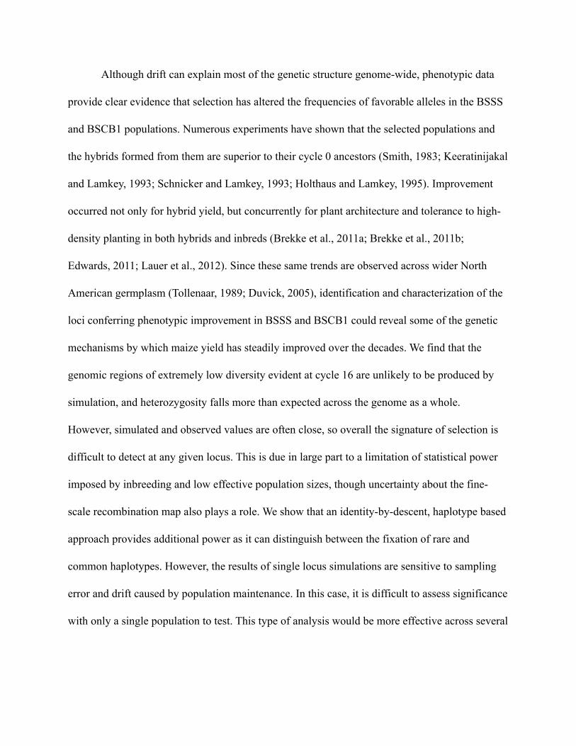
Although drift can explain most of the genetic structure genome-wide, phenotypic data

provide clear evidence that selection has altered the frequencies of favorable alleles in the BSSS

and BSCB1 populations. Numerous experiments have shown that the selected populations and

the hybrids formed from them are superior to their cycle 0 ancestors (Smith, 1983; Keeratinijakal

and Lamkey, 1993; Schnicker and Lamkey, 1993; Holthaus and Lamkey, 1995). Improvement

occurred not only for hybrid yield, but concurrently for plant architecture and tolerance to high-

density planting in both hybrids and inbreds (Brekke et al., 2011a; Brekke et al., 2011b;

Edwards, 2011; Lauer et al., 2012). Since these same trends are observed across wider North

American germplasm (Tollenaar, 1989; Duvick, 2005), identification and characterization of the

loci conferring phenotypic improvement in BSSS and BSCB1 could reveal some of the genetic

mechanisms by which maize yield has steadily improved over the decades. We find that the

genomic regions of extremely low diversity evident at cycle 16 are unlikely to be produced by

simulation, and heterozygosity falls more than expected across the genome as a whole.

However, simulated and observed values are often close, so overall the signature of selection is

difficult to detect at any given locus. This is due in large part to a limitation of statistical power

imposed by inbreeding and low effective population sizes, though uncertainty about the fine-

scale recombination map also plays a role. We show that an identity-by-descent, haplotype based

approach provides additional power as it can distinguish between the fixation of rare and

common haplotypes. However, the results of single locus simulations are sensitive to sampling

error and drift caused by population maintenance. In this case, it is difficult to assess significance

with only a single population to test. This type of analysis would be more effective across several

replicated populations, which can control for genetic drift due to the independence between the

selections in each replicate (C. Lamkey and A. Lorenz, personal communication).

van Heerwaarden et al., 2012 assessed variation and tested for selection across a wider

range of North American maize germplasm using the same SNP array. Although selected loci

were identified in that study, the overall effects on genome diversity and haplotype patterns were

relatively small compared with the impact of domestication. That study was a wide survey across

many germplasm sources. The limited impact of selection could arise because different

haplotypes and loci are selected in different breeding programs. In support of this idea, we find

that the most likely targets of selection between the BSSS and BSCB1 populations occur at non-

overlapping loci. This non-overlap between putatively selected loci in complementary

populations has also been observed in commercial breeding programs (Feng et al., 2006).

The observation that the same targets of selection are not observed in the opposing

heterotic populations bears implications for the genetic mechanisms responsible for heterosis and

the success of maize hybrids. Classic overdominance models of heterosis predict that at a single

locus, two distinct alleles confer heterozygote advantage when combined, while the dominance

model predicts that heterosis is driven by dominance effects and the complementation of linked

alleles in low-recombination regions (dominance or pseudo-overdominance). In the case of true

overdominance, we expect selection should lead to decreased heterozygosity at a locus in both

populations as complementary haplotypes are fixed in each group. We find no evidence of this

genetic phenomenon. The observed pattern instead favors a dominance model, where fixation of

a haplotype in one population simply selects against that same haplotype in the other population.

Because most deleterious alleles are rare in both heterotic groups (S. Mezmouk and J. Ross-

Ibarra, unpublished results), most haplotypes in the second population will have a different suite

of deleterious variants and will complement the fixed haplotype reasonably well such that

selection will have little impact on diversity in the second population. Our data are consistent

with such a process having been important for hybrid improvement in the Iowa RSS experiment,

and the lack of extreme differentiation seen over time across US Corn Belt germplasm is

consistent with a role for such selection in maize hybrid improvement in general (van

Heerwaarden et al., 2012).

Our results are consistent with the dominance and pseudo-overdominance models, but

we caution that the exact outcome of particular models will depend strongly on the effects of

selection, drift, and the frequencies of beneficial alleles. Disentangling these factors remains a

major challenge that will require careful simulation of maize breeding using a wider range of

parameters. This is especially true because in a model of hybrid complementation, genetic drift

in one population can alter the selective value of alleles in the other population. When drift and

selection interact in such a manner, tests for selection that attempt to independently partition the

effects of each force may not provide the full picture. Furthermore, uncertainties in the fine-scale

relationship between genetic and physical distance make it difficult to assign significance in

forward-simulation approaches. In the end, the best test for selection of specific genomic regions

will ultimately be conducted by phenotypic observation in the field in balanced tests of different

haplotypes. In the case of individual breeding programs, genome-wide genotyping such as we

conducted here can identify the lines carrying the recombinant haplotypes and introgressions

necessary to conduct such an experiment.

Table 1. Ancestry of haplotypes fixed in the cycle 16 population.

Population Chromosome

Genetic Interval

(cM)

Physical Interval

(Mb) Founder Inbred Derived Lines with HaplotypeBSSS 3 40.2-41.4 67.7-123 CI187-2 B94BSSS 3 43-48.5 129.2-157.1 NDa B89, B94BSSS 4 39.7-42.1 39.9-82.7 CI187-2 B89, B94, B67, B72, B39, B43BSSS 9 30.6-33.5 20.8-26.6 Oh7b B89, B94, B43, B17, B72, B84,

B67BSSS 9 34.3-35.6c 30.8-90.4c Os420 B89, B94

BSCB1 2 50.2-51.8 80.6-114.5 CC5 B90, B91, B95, B97, B99BSCB1 4 42.1-42.8 82.7-140 NDa B90, B95, B97BSCB1 8 46.1-50.7 125.1-145.6 P8 B90, B97, B91, B99, B54

a ND = Not Determined (Either a recombinant haplotype or originates from an un-genotyped founder)

b Although Oh7 is a BSCB1 founder, it is a descendant of CI.540, an un-genotyped BSSS founder. BSSS

segments matching Oh7 presumably derive from CI.540

c Founders Ind_B2 (BSSS), CI187-2 (BSSS), R4 (BSCB1), and I205 (BSCB1) are all IBD at this region of

chromosome 9

ACKNOWLEDGEMENTS

We thank O. S. Smith and members of the Ross-Ibarra lab for comments on earlier versions of

the manuscript. J.P.G received support for this research as a Merck Fellow of the Life Sciences

Research Foundation. This research was supported by the National Science Foundation

(IOS-0820619) and funds provided to USDA-ARS (MDM). Names of products are necessary to

report factually on available data: however, neither the USDA, nor any other participating

institution guarantees or warrants the standard of the product and the use of the name does not

imply approval of the product to the exclusion of others that may also be suitable.

LITERATURE CITED

ANDERSON, E., 1944 The sources of effective germ-plasm in hybrid maize. Annals of the

Missouri Botanical Garden 31: 355-361.

BREKKE, B., J. EDWARDS, AND A. KNAPP, 2011a Selection and Adaptation to High Plant

Density in the Iowa Stiff Stalk Synthetic Maize (L.) Population. Crop Science 51: 1965.

BREKKE, B., J. EDWARDS, AND A. KNAPP, 2011b Selection and Adaptation to High Plant

Density in the Iowa Stiff Stalk Synthetic Maize (L.) Population: II. Plant Morphology. Crop

Science 51: 2344.

CHIA, J. M., C. SONG, P. J. BRADBURY, D. COSTICH, N. DE LEON et al., 2012 Maize

HapMap2 identifies extant variation from a genome in flux. Nature Genetics 44: 803-807.

COMSTOCK, R. E., H. F. ROBINSON, AND P. H. HARVEY, 1949 A breeding procedure

designed to make maximum use of both general and specific combining ability. Agronomy

Journal 41: 360-367.

CRABB, A. R., 1947 The hybrid-corn makers: prophets of plenty. Rutgers Univ. Press, New

Brunswick.

DARRAH, L. L., AND M. S. ZUBER, 1986 1985 United States farm maize germplasm base and

commercial breeding strategies. Crop Science 26: 1109-1113.

DUVICK, D. N., 2005 The Contribution of Breeding to Yield Advances in maize (Zea mays L.).

Advances in Agronomy 86: 83-145.

DUVICK, D. N., J. S. C. SMITH, AND M. COOPER, 2004 Long-term selection in a

commercial hybrid maize breeding program. Plant Breeding Reviews 24: 109-152.

EDWARDS, J., 2011 Changes in Plant Morphology in Response to Recurrent Selection in the

Iowa Stiff Stalk Synthetic Maize Population. Crop Science 51: 2352.

FENG, L., S. SEBASTIAN, S. SMITH, AND M. COOPER, 2006 Temporal trends in SSR allele

frequencies associated with long-term selection for yield of maize. Maydica 51: 293.

GANAL, M. W., G. DURSTEWITZ, A. POLLEY, A. BERARD, E. S. BUCKLER et al., 2011 A

large maize (Zea mays L.) SNP genotyping array: development and germplasm genotyping, and

genetic mapping to compare with the B73 reference genome. PLoS One 6: e28334.

GERDES, J. T., W. F. TRACY, J. G. COORS, J. L. GEADLEMANN, AND M. K. VINEY, 1993

Compilation of North American maize breeding germplasm. Crop Science Society of America,

Madison, Wisconsin.

HAGDORN, S., K. R. LAMKEY, M. FRISCH, P. E. O. GUIMARAES, AND A. E.

MELCHINGER, 2003 Molecular genetic diversity among progenitors and derived elite lines of

BSSS and BSCB1 maize populations. Crop Science 43: 474-482.

HINZE, L. L., S. KRESOVICH, J. D. NASON, AND K. R. LAMKEY, 2005 Population Genetic

Diversity in a Maize Reciprocal Recurrent Selection Program. Crop Science 45: 2435-2442.

HO, J. C., S. KRESOVICH, AND K. R. LAMKEY, 2005 Extent and distribution of genetic

variation in US maize: Historically important lines and their open-pollinated dent and flint

progenitors. Crop Science 45: 1891-1900.

HOLTHAUS, J. F., AND K. R. LAMKEY, 1995 Population means and genetic variances in

selected and unselected Iowa Stiff Stalk Synthetic maize populations. Crop Science 35:

1581-1589.

HUDSON, R. R., D. D. BOOS, AND N. L. KAPLAN, 1992 A statistical test for detecting

geographic subdivision. Molecular Biology and Evolution 9: 138-151.

HUFFORD, M. B., X. XU, J. VAN HEERWAARDEN, T. PYHAJARVI, J. M. CHIA et al., 2012

Comparative population genomics of maize domestication and improvement. Nature Genetics

44: 808-811.

KEERATINIJAKAL, V., AND K. R. LAMKEY, 1993 Responses to reciprocal recurrent

selection in BSSS and BSCB1 maize populations. Crop Science 33: 73-77.

LABATE, J. A., K. R. LAMKEY, M. LEE, AND W. L. WOODMAN, 1997 Molecular genetic

diversity after reciprocal recurrent selection in BSSS and BSCB1 maize populations. Crop

Science 37: 416-423.

LAUER, S., B. D. HALL, E. MULAOSMANOVIC, S. R. ANDERSON, B. NELSON et al.,

2012 Morphological Changes in Parental Lines of Pioneer Brand Maize Hybrids in the US

Central Corn Belt. Crop Science 52: 1033-1043.

LEE, M., N. SHAROPOVA, W. D. BEAVIS, D. GRANT, M. KATT et al., 2002 Expanding the

genetic map of maize with the intermated B73× Mo17 (IBM) population. Plant Molecular

Biology 48: 453-461.

MCMULLEN, M. D., S. KRESOVICH, H. S. VILLEDA, P. BRADBURY, H. LI et al., 2009

Genetic properties of the maize nested association mapping population. Science 325: 737-740.

MCVEAN, G., 2009 A genealogical interpretation of principal components analysis. PLoS

Genetics 5: e1000686.

MESSMER, M. M., A. E. MELCHINGER, M. LEE, W. L. WOODMAN, E. A. LEE et al., 1991

Genetic diversity among progenitors and elite lines from the Iowa Stiff Stalk Synthetic (BSSS)

maize population: comparison of allozyme and RFLP data. Theoretical and Applied Genetics 83:

97-107.

PENNY, L. H., AND S. A. EBERHART, 1971 Twenty years of reciprocal recurrent selection

with two synthetic varieties of maize (Zea mays L.). Crop Science 11: 900-903.

ROMAY, M. C., A. BUTRÓN, A. ORDÁS, P. REVILLA, AND B. ORDÁS, 2012 Effect of

Recurrent Selection on the Genetic Structure of Two Broad-Based Spanish Maize Populations.

Crop Science 52: 1493-1502.

SAGHAI-MAROOF, M. A., K. M. SOLIMAN, R. A. JORGENSEN, AND R. W. ALLARD,

1984 Ribosomal DNA spacer-length polymorphisms in barley: Mendelian inheritance,

chromosomal location, and population dynamics. Proceedings of the National Academy of

Sciences 81: 8014-8018.

SCHEET, P., AND M. STEPHENS, 2006 A fast and flexible statistical model for large-scale

population genotype data: applications to inferring missing genotypes and haplotypic phase. The

American Journal of Human Genetics 78: 629-644.

SCHNABLE, P. S., D. WARE, R. S. FULTON, J. C. STEIN, F. WEI et al., 2009 The B73 maize

genome: complexity, diversity, and dynamics. Science 326: 1112-1115.

SCHNICKER, B. J., AND K. R. LAMKEY, 1993 Interpopulation genetic variance after

reciprocal recurrent selection in BSSS and BSCB1 maize populations. Crop Science 33: 90-95.

SENIOR, M. L., J. P. MURPHY, M. M. GOODMAN, AND C. W. STUBER, 1998 Utility of

SSRs for determining genetic similarities an relationships in maize using an agarose gel system.

Crop Science 38: 1088-1098.

SMITH, O. S., 1983 Evaluation of recurrent selection in BSSS, BSCB1, and BS13 maize

populations. Crop Science 23: 35-40.

THORNTON, K., 2003 Libsequence: a C++ class library for evolutionary genetic analysis.

Bioinformatics 19: 2325-2327.

TOLLENAAR, M., 1989 Genetic improvement in grain yield of commercial maize hybrids

grown in Ontario from 1959 to 1988. Crop Science 29: 1365-1371.

TRACY, W. F., AND M. A. CHANDLER, 2006 The historical and biological basis of the

concept of heterotic patterns in corn belt dent maize. Plant Breeding: The Arnel R. Hallauer

International Symposium: 219-233.

TROYER, A. F., 1999 Background of US hybrid corn. Crop Science 39: 601-626.

VAN HEERWAARDEN, J., M. B. HUFFORD, AND J. ROSS-IBARRA, 2012 Historical

genomics of North American maize. Proceedings of the National Academy of Sciences 109:

12420-12425.

WICKHAM, H., 2009 ggplot2: elegant graphics for data analysis. Springer Publishing

Company, Incorporated,

WINKLER, C. R., N. M. JENSEN, M. COOPER, D. W. PODLICH, AND O. S. SMITH, 2003

On the determination of recombination rates in intermated recombinant inbred populations.

Genetics 164: 741-745.

FIGURE LEGENDS

Figure 1. Principal component analysis of the SNP data from Iowa RRS. The axes represent the

first two eigenvectors from an analysis of cycles 0-16, with projection of the founder lines onto

the vector space. The variation explained by each eigenvector is given in parentheses on the axes.

The populations steadily diverge at increasing cycles, with less distinction visible between the

founder groups. The comparatively large distance between cycles 4 and 8 corresponds to a

switch from one to two generations of selfing at each cycle. The smaller separation between

cycles 8-16 corresponds to an increase in effective population size from ten to twenty. The BSSS

cycle 0 population has drifted away from the BSSS founders, despite the absence of intentional

selection during the creation and maintenance of cycle 0.

Figure 2. Heterozygosity and FST across cycles. H (left panel) and FST (right panel) plotted as a

function of selection cycle in each population.

Figure 3. Heterozygosity (H) at cycle16 across all ten chromosomes in each population. H

is calculated on 15-marker sliding windows with 5 marker steps. Each point is plotted at the

midpoint of the 15-marker window.

Figure 4. Heterozygosity (H) across chromosome 9 in each cycle of BSSS plotted on the

physical (A) or genetic (B) map. H is calculated on 15-marker sliding windows, with 5 marker

steps between each calculation. Each data point is color-coded based on a linear transformation

of recombination rate (red = low recombination rate). Shaded regions represent 2 cM windows

found to have heterozygosity values significantly lower than expected by simulation at a given

cycle. Light shading denotes significance at P < 0.0025, whereas the darker shading represents

significance at P < 0.001. Comparing the physical and genetic maps reveals that the regions of

fixation are extremely small genetically, but some contain much of the physical content of the

chromosome.

Figure 5. Heterozygosity (H) across chromosome 4 in each cycle of BSCB1 plotted on the

physical (A) or genetic (B) map. H is calculated on 15 marker-sliding windows, with 5 marker

steps between each calculation. Each data point is color-coded based on a linear transformation

of recombination rate (red = low recombination rate). Shaded regions represent 2 cM windows

found to have heterozygosity values significantly lower than expected by simulation at a given

cycle. Light shading denotes significance at P < 0.0025, whereas the darker shading represents

significance at P < 0.001.

Figure S1. Heterozygosity in each population, observed vs. simulated data. Heterozygosity

was calculated as the average across all markers genome-wide in the BSSS (A) and BSCB1 (B)

populations. The observed data is marked by the red line, the simulations by gray dots, and the

median of the simulations by a green dot.

Figure S2. Heterozygosity (H) at cycle16 across all ten chromosomes in each population,

calculated on 15-marker sliding windows with 5 marker steps as in Figure 3. Heterozygosity

values in BSSS (blue dots) and BSCB1 (red dots) are superimposed in one panel. 2 cM windows

of low heterozygosity that were reproduced in less than 10 of 10,000 simulations (P<0.001) are

shaded in light blue (BSSS) or pink (BSCB). At this cutoff, there is no overlap between

highlighted windows in the two populations. (A) Physical map. (B) Genetic map.

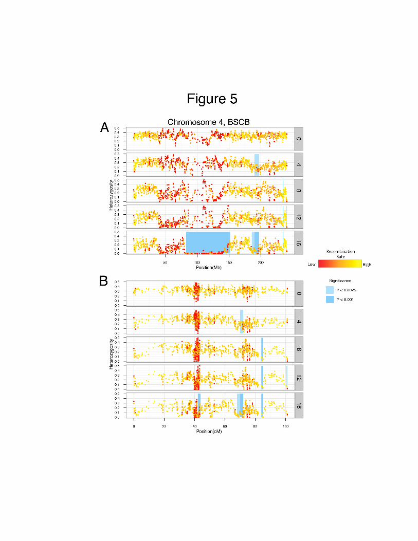
Table S1. Plants and Lines Genotyped in this study.Backgrounds of the founder inbreds are from Hagdorn et al. 2003.

Plants from the selection cyclesPlants from the selection cyclesPlants from the selection cyclesPlants from the selection cyclesPopulation Cycle # plants  

BSSS 0 34BSSS 4 36BSSS 8 35BSSS 12 36BSSS 16 36

BSCB1 0 36BSCB1 4 36BSCB1 8 35BSCB1 12 36BSCB1 16 36

BSSS Founders GenotypedBSSS Founders GenotypedBSSS Founders GenotypedBSSS Founders GenotypedInbred Background / PedigreeBackground / PedigreeBackground / Pedigree

Ind_Tr9_1_1_6 Reid Early Dent (Troyer Strain)Reid Early Dent (Troyer Strain)Reid Early Dent (Troyer Strain)Oh3167B Echelberger ClarageEchelberger ClarageEchelberger Clarage

I224 IodentIodentIodentInd467(744) Reid MediumReid MediumReid Medium

CI.187-2 Krug-Nebraska Reid x IA Gold MineKrug-Nebraska Reid x IA Gold MineKrug-Nebraska Reid x IA Gold MineOs420 Osterland Yellow DentOsterland Yellow DentOsterland Yellow DentI159 IodentIodentIodent

A3G-3-1-3 BL345BxIAI129BL345BxIAI129BL345BxIAI129Ind_Fe2_1073* Troyer Reid (Early)Troyer Reid (Early)Troyer Reid (Early)

Ill_Hy IL High YieldIL High YieldIL High YieldIll_12E unknownunknownunknown

Ind_AH83 Funk 176AFunk 176AFunk 176AInd_B2* Troyer Reid (Late Butler), parent of a founderTroyer Reid (Late Butler), parent of a founderTroyer Reid (Late Butler), parent of a founder

LE23 IL Low EarIL Low EarIL Low Ear*Parents of unavailable line F1B1*Parents of unavailable line F1B1

BSCB1 Founders GenotypedBSCB1 Founders GenotypedBSCB1 Founders GenotypedBSCB1 Founders GenotypedInbred Background / PedigreeBackground / PedigreeBackground / PedigreeI205 IodentIodentIodent

Oh51A [(OH56xWf9)Oh56] (Wooster Clarage x ?)[(OH56xWf9)Oh56] (Wooster Clarage x ?)[(OH56xWf9)Oh56] (Wooster Clarage x ?)A340 4-29 x 64 (Silver King x Northwestern Dent)4-29 x 64 (Silver King x Northwestern Dent)4-29 x 64 (Silver King x Northwestern Dent)Ill_Hy IL High YieldIL High YieldIL High YieldOh33 ClarageClarageClarageOh07 C.I.540xIII.LC.I.540xIII.LC.I.540xIII.L

R4 Funk Yellow DentFunk Yellow DentFunk Yellow DentOh40B eight line LSC compositeeight line LSC compositeeight line LSC composite

P8 Palin ReidPalin ReidPalin ReidL317 LSCLSCLSCCC5 Golden Glow (W23)Golden Glow (W23)Golden Glow (W23)

Founders not analyzedFounders not analyzedFounders not analyzedFounders not analyzedInbred Group ReasonReasonCI.540 BSSS heterozygous genotypeheterozygous genotypeF1B1 BSSS unavailableunavailableCI.617 BSSS unavailableunavailableWD456 BSSS unavailableunavailableK230 BSCB1 source segregates phenotypicallysource segregates phenotypically

Derived Lines UsedDerived Lines UsedDerived Lines UsedDerived Lines UsedInbred Group Cycle NotesB10 BSSS 0thrown out; poor data qualityB42 BSCB1 0B14A BSSS 0Cuzco x B14B43 BSSS 0B10 BSSS 0B37 BSSS 0B44 BSSS 0B17 BSSS 0B69 BSSS 0B39 BSSS 0B90 BSCB1 7B40 BSSS 0B54 BSCB1 0B78 BSSS 8from half-sib recurrent selection programB72 BSSS 3from half-sib recurrent selection programB84 BSSS 7from half-sib recurrent selection programB94 BSSS 8B99 BSCB1 10B11 BSSS 0B89 BSSS 7B95 BSCB1 7B91 BSCB1 8B67 BSSS 0B73 BSSS 5from half-sib recurrent selection programB97 BSCB1 9

Table S2. Evidence of minor contamination between cycles 4 and 8 in BSSS.

SNPS polymorphic in cycle: But not cycle: in BSSS in BSCB14 0 290 2258 0 2242 319

12 0 1227 18116 0 344 1288 4 4499 1081

12 4 2328 66916 4 551 47712 8 1821 140516 8 178 99716 12 542 6660 Founders 1202 17074 Founders 822 8858 Founders 1201 798

12 Founders 816 55016 Founders 445 460

Heterozygosity (H) of SNPS present in cycle 8 but not cycle 4Heterozygosity (H) of SNPS present in cycle 8 but not cycle 4Heterozygosity (H) of SNPS present in cycle 8 but not cycle 4Statistic BSSS BSCB

Mean 0.052 0.052Median 0.028 0.028

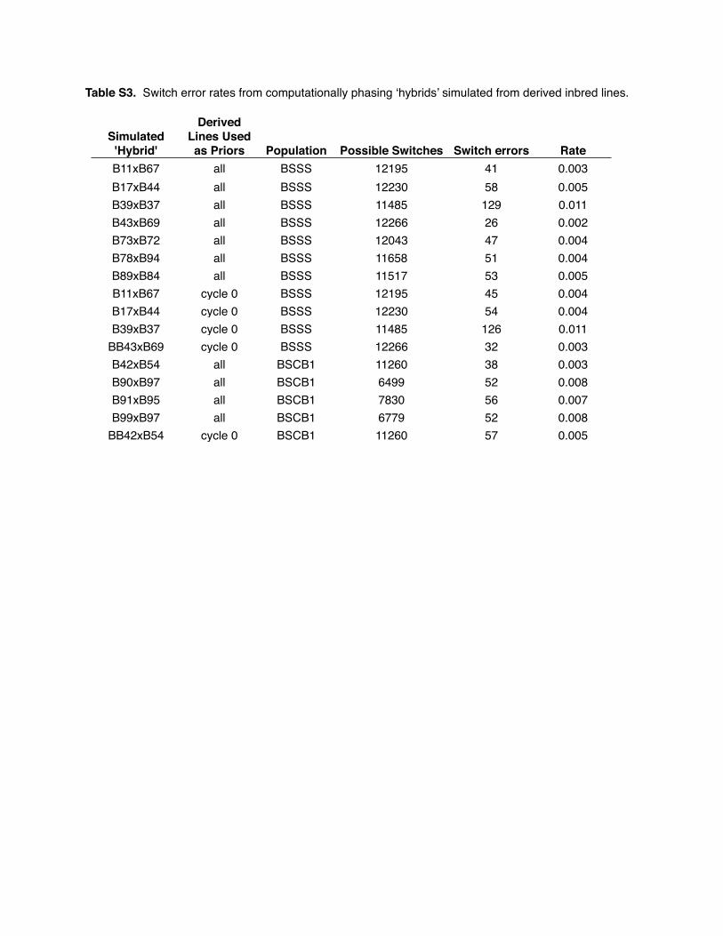
Table S3. Switch error rates from computationally phasing ‘hybrids’ simulated from derived inbred lines.

Simulated 'Hybrid'

Derived Lines Used as Priors Population Possible Switches Switch errors Rate

B11xB67 all BSSS 12195 41 0.003B17xB44 all BSSS 12230 58 0.005B39xB37 all BSSS 11485 129 0.011B43xB69 all BSSS 12266 26 0.002B73xB72 all BSSS 12043 47 0.004B78xB94 all BSSS 11658 51 0.004B89xB84 all BSSS 11517 53 0.005B11xB67 cycle 0 BSSS 12195 45 0.004B17xB44 cycle 0 BSSS 12230 54 0.004B39xB37 cycle 0 BSSS 11485 126 0.011

BB43xB69 cycle 0 BSSS 12266 32 0.003B42xB54 all BSCB1 11260 38 0.003B90xB97 all BSCB1 6499 52 0.008B91xB95 all BSCB1 7830 56 0.007B99xB97 all BSCB1 6779 52 0.008

BB42xB54 cycle 0 BSCB1 11260 57 0.005