The general linear model and Statistical Parametric Mapping · The general linear model and...

The general linear model and Statistical Parametric Mapping

I: Introduction to the GLM

The general linear model and The general linear model and Statistical Parametric MappingStatistical Parametric Mapping

I: Introduction to the GLMI: Introduction to the GLM

AlexaAlexa MorcomMorcom

and Stefan and Stefan KiebelKiebel, , RikRik Henson, Andrew Henson, Andrew Holmes & JHolmes & J--B B PolinePoline

• Introduction• Essential concepts

– Modelling– Design matrix– Parameter estimates – Simple contrasts

• Summary

Overview

Some terminology

• SPM is based on a mass univariate approach that fits a model at each voxel– Is there an effect at location X? Investigate localisation of

function or functional specialisation

– How does region X interact with Y and Z? Investigate behaviour of networks or functional integration

• A General(ised) Linear Model– Effects are linear and additive

– If errors are normal (Gaussian), General (SPM99)

– If errors are not normal, Generalised (SPM2)

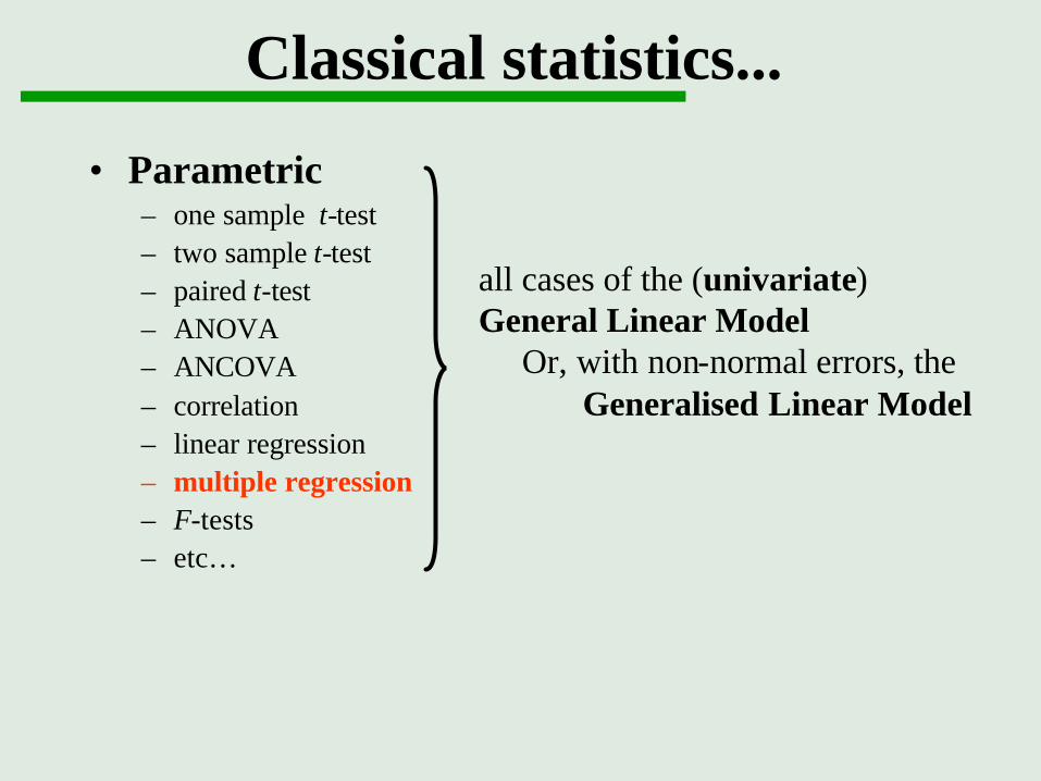
• Parametric– one sample t-test– two sample t-test– paired t-test– ANOVA– ANCOVA– correlation– linear regression– multiple regression– F-tests– etc…

all cases of the (univariate) General Linear Model

Or, with non-normal errors, the Generalised Linear Model

Classical statistics...


• Multivariate?




→ PCA/ SVD, MLM


• Multivariate?• Non-parametric?



→ SnPM


→ PCA/ SVD, MLM

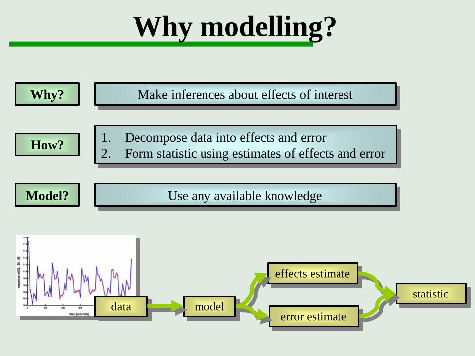
1. Decompose data into effects and error2. Form statistic using estimates of effects and error

1. Decompose data into effects and error2. Form statistic using estimates of effects and error

Make inferences about effects of interestMake inferences about effects of interestWhy?

How?

Use any available knowledgeUse any available knowledgeModel?

datadata modelmodel

effects estimateeffects estimate

error estimateerror estimate

statisticstatistic

Why modelling?

VarianceVariance BiasBias

No smoothingNo smoothing

No normalisationNo normalisation

Massive modelMassive model

but ... not much sensitivity

but ... not much sensitivity

Captures signal

Lots of smoothingLots of smoothing

Lots of normalisationLots of normalisation

Sparse modelSparse model

but ... may misssignal

but ... may misssignal

High sensitivity

A very general model

A very general model

defaultSPM

defaultSPM

Choose your model“All models are wrong, but some are useful”

George E.P.Box

Modelling with SPM

PreprocessingPreprocessing SPMsSPMs

Functional dataFunctional data

TemplatesTemplates

Smoothednormalised

data

Smoothednormalised

data

Design matrixDesign matrix

Variance componentsVariance components

ContrastsContrasts

ThresholdingThresholding

Parameterestimates

ParameterestimatesGeneralised

linearmodel

Generalisedlinearmodel

Modelling with SPM



Preprocessed data: single

voxel

Preprocessed data: single

voxel

Design matrixDesign matrix

Variance componentsVariance components

SPMsSPMs

ContrastsContrasts

Parameterestimates

Parameterestimates

Passive word listeningversus rest

Passive word listeningversus rest

7 cycles of rest and listening

7 cycles of rest and listening

Each epoch 6 scanswith 7 sec TR

Each epoch 6 scanswith 7 sec TR

Question: Is there a change in the BOLD response between listening and rest?


Time series of BOLD responses in one voxel

Time series of BOLD responses in one voxel

Stimulus functionStimulus function

One sessionOne session

fMRI example

GLM essentials

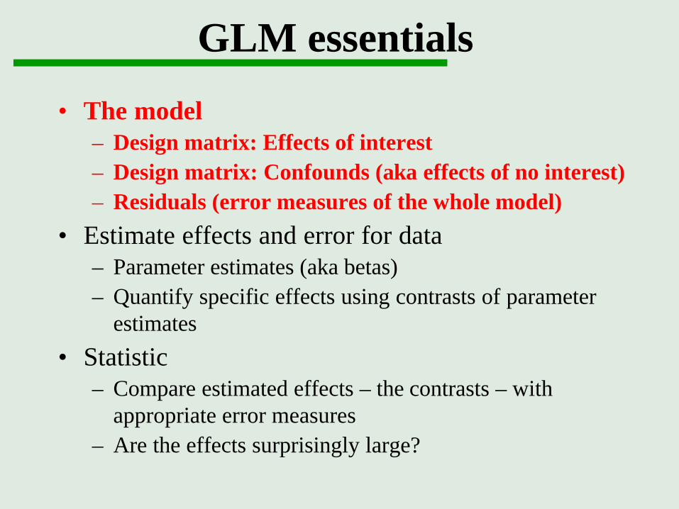
• The model– Design matrix: Effects of interest– Design matrix: Confounds (aka effects of no interest)– Residuals (error measures of the whole model)

• Estimate effects and error for data– Parameter estimates (aka betas)– Quantify specific effects using contrasts of parameter

estimates

• Statistic – Compare estimated effects – the contrasts – with

appropriate error measures– Are the effects surprisingly large?

Intensity

Tim

e

Regression model

= β1 β2+ + erro

r

x1 x2 ε

ε∼Ν(0, σ2Ι)(error is normal andindependently and

identically distributed)



Hypothesis test: β1 = 0?(using t-statistic)

General case

Regression model

= + +1β 2β

Y + ε+= 11xβ 22ˆ xβ

Model is specified by1. Design matrix X2. Assumptions about ε

Model is specified by1. Design matrix X2. Assumptions about ε

General case

Matrix formulation

Yi = β1 xi + β2 + εi i = 1,2,3

Y1 x1 1 β1 ε1Y2= x2 1 + ε2Y3 x3 1 β1 ε3

Y = X β + ε

Y1 = β1 x1 + β2 × 1 + ε1

Y2 = β1 x2 + β2 × 1 + ε2

Y3 = β1 x3 + β2 × 1 + ε3

dummy variables

Matrix formulation

Yi = β1 xi + β2 + εi i = 1,2,3

Y1 x1 1 β1 ε1Y2= x2 1 + ε2Y3 x3 1 β1 ε3

Y = X β + ε

Y1 = β1 x1 + β2 × 1 + ε1

Y2 = β1 x2 + β2 × 1 + ε2

Y3 = β1 x3 + β2 × 1 + ε3

dummy variables

x

y

××

×

β2^

β11

Linear regression

Parameter estimates β1 & β2

Fitted values Y1 & Y2

Residuals ε1 & ε2

^ ^

^ ^

^ ^

Yi

Yi^

Hats = estimates

Hats = estimates

^

Y = β1 × X1 +β2 × X2 + ε

(1,1,1)

(x1, x2, x3)X1

X2O

Y1 x1 1 β1 ε1Y2 = x2 1 + ε2Y3 x3 1 β2 ε3

DATA(Y1, Y2, Y3)

Y

design space

Geometrical perspective

GLM essentials


• Estimate effects and error for data– Parameter estimates (aka betas)– Quantify specific effects using contrasts of

parameter estimates



Parameter estimation

εβ += XY

Estimate parametersEstimate parameters

such that such that ∑=

N

tt

1

2ε minimalminimal

βε ˆˆ XY −=

residualsresiduals

Least squaresparameter estimate

Least squaresparameter estimate

YXXX TT 1)(ˆ −=β

Parameter estimates

Parameter estimates

Ordinary least squares

Parameter estimation

εβ += XY

βε ˆˆ XY −=

residuals = rresiduals = r

YXXX TT 1)(ˆ −=β

Parameter estimates

Parameter estimates

Error variance σ2 = (sum of) squared residuals standardised for df

= rTr / df (sum of squares)…where degrees of freedom df (assuming iid):

= N - rank(X)(=N-P if X full rank)

Error variance σ2 = (sum of) squared residuals standardised for df

= rTr / df (sum of squares)…where degrees of freedom df (assuming iid):

= N - rank(X)(=N-P if X full rank)

Ordinary least squares

Y = β1 × X1 +β2 × X2 + ε

(1,1,1)

(x1, x2, x3)X1

X2O

Y1 x1 1 β1 ε1Y2 = x2 1 + ε2Y3 x3 1 β2 ε3

Y

design space

Estimation (geometrical)

(Y1,Y2,Y3)^ ^ ^Y

ε = (ε1,ε2,ε3)T^ ^ ^^

DATA(Y1, Y2, Y3)

RESIDUALS

GLM essentials


• Estimate effects and error for data– Parameter estimates (aka betas)– Quantify specific effects using contrasts of parameter

estimates



Inference - contrasts

εβ += XY A contrast = a linear combination of parameters: c´ x β à spm_con*img

boxcar parameter > 0 ?boxcar parameter > 0 ?

Null hypothesis:Null hypothesis: 01 =β

t-test: one-dimensional contrast, difference in means/ difference from zero

Does boxcar parameter model anything?

Does boxcar parameter model anything?

Null hypothesis: variance of tested effects = error variance

Null hypothesis: variance of tested effects = error variance

F-test: tests multiple linear hypotheses – does subset of model account for significant variance

à spmT_000*.imgSPM{t} map

à ess_000*.imgSPM{F} map

t-statistic - example

εβ += XY

c = 1 0 0 0 0 0 0 0 0 0 0c = 1 0 0 0 0 0 0 0 0 0 0)ˆ(ˆ

ˆ

ββT

T

cdtSc

t =

X Standard error of contrast depends on the design, and is larger with greater residual error and

‚greater‘ covariance/ autocorrelation

Degrees of freedom d.f. then = n-p, where nobservations, p parameters

Standard error of contrast depends on the design, and is larger with greater residual error and

‚greater‘ covariance/ autocorrelation

Degrees of freedom d.f. then = n-p, where nobservations, p parameters

Contrast of parameter estimates

Contrast of parameter estimates

Variance estimateVariance estimate

Tests for a directional difference in means

Tests for a directional difference in means

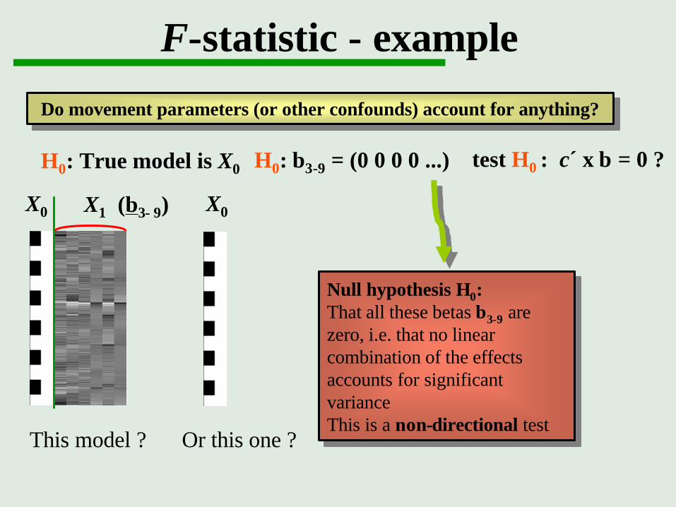
F-statistic - example

Null hypothesis H0:That all these betas β3-9 are zero, i.e. that no linear combination of the effects accounts for significant varianceThis is a non-directional test

Null hypothesis H0:That all these betas β3-9 are zero, i.e. that no linear combination of the effects accounts for significant varianceThis is a non-directional test

H0: β3-9 = (0 0 0 0 ...) test H0 : c´ x β = 0 ?H0: True model is X0

This model ? Or this one ?

Do movement parameters (or other confounds) account for anything?Do movement parameters (or other confounds) account for anything?

X1 (β3−9)X0 X0

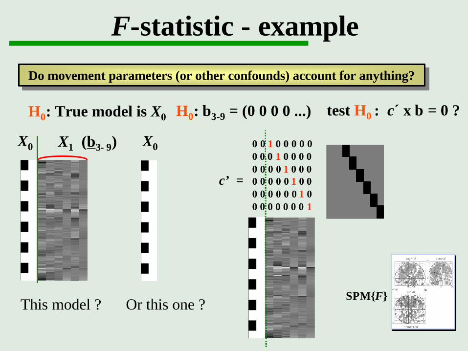
H0: β3-9 = (0 0 0 0 ...)

0 0 1 0 0 0 0 0 0 0 0 1 0 0 0 00 0 0 0 1 0 0 00 0 0 0 0 1 0 00 0 0 0 0 0 1 00 0 0 0 0 0 0 1

c’ =

SPM{F}

test H0 : c´ x β = 0 ?H0: True model is X0

F-statistic - example

Do movement parameters (or other confounds) account for anything?Do movement parameters (or other confounds) account for anything?

X1 (β3−9)X0

This model ? Or this one ?

X0

Summary so far

• The essential model contains – Effects of interest

• A better model?– A better model (within reason) means smaller residual

variance and more significant statistics– Capturing the signal – later– Add confounds/ effects of no interest– Example of movement parameters in fMRI– A further example (mainly relevant to PET)…

Example PET experimentβ1 β2 β3 β4

rank

(X)=

3

12 scans, 3 conditions (1-way ANOVA)yj = x1j b1 + x2j b2 + x3j b3 + x4j b4 + ej

where (dummy) variables:x1j = [0,1] = condition A (first 4 scans)x2j = [0,1] = condition B (second 4 scans)x3j = [0,1] = condition C (third 4 scans)x4j = [1] = grand mean (session constant)

12 scans, 3 conditions (1-way ANOVA)yj = x1j b1 + x2j b2 + x3j b3 + x4j b4 + ej

where (dummy) variables:x1j = [0,1] = condition A (first 4 scans)x2j = [0,1] = condition B (second 4 scans)x3j = [0,1] = condition C (third 4 scans)x4j = [1] = grand mean (session constant)

Global effects

• May be variation in PET tracer dose from scan to scan

• Such “global” changes in image intensity (gCBF) confound local / regional (rCBF) changes of experiment

• Adjust for global effects by:- AnCova (Additive Model) - PET?- Proportional Scaling - fMRI?

• Can improve statistics when orthogonal to effects of interest…

• …but can also worsen when effects of interest correlated with global

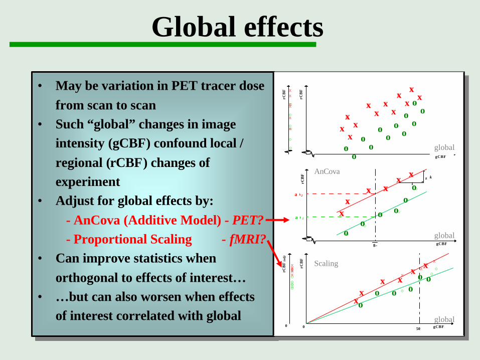
• May be variation in PET tracer dose from scan to scan

• Such “global” changes in image intensity (gCBF) confound local / regional (rCBF) changes of experiment

• Adjust for global effects by:- AnCova (Additive Model) - PET?- Proportional Scaling - fMRI?

• Can improve statistics when orthogonal to effects of interest…

• …but can also worsen when effects of interest correlated with global

rCB

F

x

o

o

o

o

o

o

x

x

x

x

x

gCBF

rCB

F

x

o

o

o

o

o

o

x

x

x

x

x

global

gCBF

rCB

F

x

o

o

o

o

o

o

x

x

x

x

x

g..

α k 1

α k 2

ζ k

1

global

AnCova

globalgCBF

rCB

F

x

oo

o

oo

o

xx

xx

x

0 50

rCB

F (a

dj)

o

0

xxxx

xxooooo

Scaling

xx

x xx

x

oo

o oo

o

xx

x xx x

oo

o oo

o

xx

x xx

x

oo o o

o o

xx

x xx

x

oo

o oo

o

Global effects (AnCova)β1 β2 β3 β4 β5

rank

(X)=

4

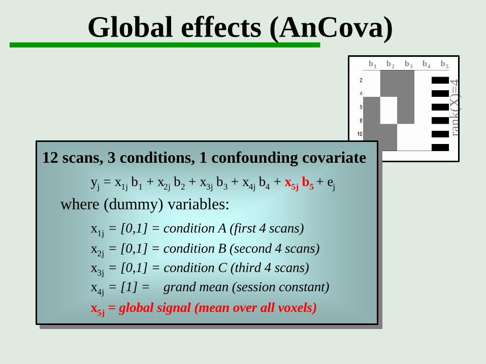
12 scans, 3 conditions, 1 confounding covariateyj = x1j b1 + x2j b2 + x3j b3 + x4j b4 + x5j b5 + ej

where (dummy) variables:x1j = [0,1] = condition A (first 4 scans)x2j = [0,1] = condition B (second 4 scans)x3j = [0,1] = condition C (third 4 scans)x4j = [1] = grand mean (session constant)x5j = global signal (mean over all voxels)

12 scans, 3 conditions, 1 confounding covariateyj = x1j b1 + x2j b2 + x3j b3 + x4j b4 + x5j b5 + ej

where (dummy) variables:x1j = [0,1] = condition A (first 4 scans)x2j = [0,1] = condition B (second 4 scans)x3j = [0,1] = condition C (third 4 scans)x4j = [1] = grand mean (session constant)x5j = global signal (mean over all voxels)

rank

(X)=

4

β1 β2 β3 β4 β5

• Global effects not accounted for

• Maximum degrees of freedom (global uses one)

• Global effects not accounted for

• Maximum degrees of freedom (global uses one)

Global effects (AnCova)

• Global effects independent of effects of interest

• Smaller residual variance

• Larger T statistic• More significant

• Global effects independent of effects of interest

• Smaller residual variance

• Larger T statistic• More significant

• Global effects correlated with effects of interest

• Smaller effect &/or larger residuals

• Smaller T statistic• Less significant

• Global effects correlated with effects of interest

• Smaller effect &/or larger residuals

• Smaller T statistic• Less significant

No GlobalNo Global Correlated globalCorrelated globalOrthogonal globalOrthogonal global

β1 β2 β3 β4

rank

(X)=

3

β1 β2 β3 β4 β5

rank

(X)=

4

• Two types of scaling: Grand Mean scaling and Global scaling- Grand Mean scaling is automatic, global scaling is optional- Grand Mean scales by 100/mean over all voxels and ALL scans

(i.e, single number per session) - Global scaling scales by 100/mean over all voxels for EACH scan

(i.e, a different scaling factor every scan)• Problem with global scaling is that TRUE global is not (normally)

known… … only estimated by the mean over voxels- So if there is a large signal change over many voxels, the global

estimate will be confounded by local changes- This can produce artifactual deactivations in other regions after

global scaling• Since most sources of global variability in fMRI are low frequency

(drift), high-pass filtering may be sufficient, and many people do not use global scaling

• Two types of scaling: Grand Mean scaling and Global scaling- Grand Mean scaling is automatic, global scaling is optional- Grand Mean scales by 100/mean over all voxels and ALL scans

(i.e, single number per session) - Global scaling scales by 100/mean over all voxels for EACH scan

(i.e, a different scaling factor every scan)• Problem with global scaling is that TRUE global is not (normally)

known… … only estimated by the mean over voxels- So if there is a large signal change over many voxels, the global

estimate will be confounded by local changes- This can produce artifactual deactivations in other regions after

global scaling• Since most sources of global variability in fMRI are low frequency

(drift), high-pass filtering may be sufficient, and many people do not use global scaling

Global effects (scaling)

Summary

• General(ised) linear model partitions data into– Effects of interest & confounds/ effects of no interest– Error

• Least squares estimation – Minimises difference between model & data– To do this, assumptions made about errors – more later

• Inference at every voxel– Test hypothesis using contrast – more later– Inference can be Bayesian as well as classical

• Next: Applying the GLM to fMRI

The general linear model and Statistical Parametric Mapping · The general linear model and...

Documents

Transcript of The general linear model and Statistical Parametric Mapping · The general linear model and...