The Future of Rural School Research and Development: Methodological

Innovations for the Next Generation

James A. Bovaird

University of Nebraska-Lincoln

Special Thanks

• Members of the CYFS Statistics & Research Methodology Unit: – Dr. Greg Welch, Dr. Leslie Shaw, Natalie Koziol, Frances Chumney,

Chaorong Wu, Carina McCormick, Ann Arthur, Elizabeth Timberlake

– Dr. Kevin Kupzk, University of Nebraska Medical Center

– Dr. Michael Toland, University of Kentucky

• Colleagues in the National Center for Research on Rural Education

Central Tenets

• Rural education research has and will continue to overcome perceived limitations to true experimentation, yet still approximate the level of knowledge available through random assignment and explicit environmental control.

• Educational policy must be utilitarian, consequently, research impacting educational policy in rural settings must focus on systems-level applications.

• Viable solutions exist in other disciplines and can be translated to rural education research.

Topics to be Discussed Today

• Operational definition of "rural" and its impact on inferences

• Preserving and featuring the uniqueness of rural settings in systems level investigations through advanced statistical modeling

• Quasi-experimentation as an alternative to traditional random assignment

• Efficiency of measurement paradigms to reduce the amount of data necessary for valid inferences

• Innovations in small sample inferential testing

Measuring “Rural”

Some Classifications Schemes Can Get Ugly

This part of the presentation is meant to help make sense of some of the most common systems & their implications.

Establishing Organization

(Researcher)Classification

Unit (Level) of

Classification Description

Office of Management &

Budget (OMB)

Metropolitan and

Micropolitan Statistical

Areas

County

METRO: Areas are based on the presence of an urbanized

area with a population of at least 50,000.

MICRO: Areas are defined as an urban cluster with a

population of at least 10,000 but no more than 50,000.

Counties that do not fit into either of these definitions are

classified as "Outside Core Based Statistical Areas."

United States Census Bureau

(Census)

Urban (Urbanized

Areas or Urban

Clusters) and Rural

Census tract

and/or block

(county based)

URBAN: Urbanized Areas are defined as having 50,000 or

more people and Urban Clusters at least 2,500 and less than

50,000 people.

RURAL: Rural areas consist of all territory located outside of

urbanized areas and urban clusters, thus populations of fewer

than 2,500 residents.

National Center for Education

Statistics (NCES)

Urban-Centric Locale

Codes

School and school-

district

Urban-centric locale codes are based on a combination of

proximity to an urbanized area and population size. School

districts are classified based on the locale code at which the

majority of the district's students are enrolled.

Economic Research Service,

United States Department of

Agriculture (USDA)

Urban Influence Codes County

The OMB's metropolitan and micropolitan statistical areas

are divided into smaller groups based on population,

adjacency to metro areas, and commuting patterns.

Economic Research Service,

United States Department of

Agriculture (USDA)

Rural-Urban Commuting

Area (RUCA)

Census tract and

ZIP code

RUCA codes combine measures of population density,

urbanization, and commuting patterns at the census tract and

ZIP code levels. Coding scheme enables researchers to

create both primary and secondary codes for areas.

Current Work

• Summary and synthesis of current coding strategies

• Empirical evaluation of the impact of different coding strategies

• Empirical evaluation of continuous variable and latent variable approaches to modeling rurality

Modeling the Rural Context

Kansas Kindergarten Readiness Project: Student Readiness for School

• Cross-sectional contextual (county) model of (student) school readiness – Bovaird (2005); Bovaird,

Martinez, & Stuber (2006)

– Multilevel model is appropriate • students nested within

county

• Goal: – To describe the relationship

between county-level contextual characteristics and kindergarten preparedness, controlling for student-level characteristics.

Kansas Kindergarten Readiness Project: The Measures

• Kansas School Entry Assessment

– Teacher-completed measure of kindergarten preparedness

– 41 items in 6 areas of school readiness: symbolic development (Sy), literacy development (Li), mathematical knowledge (Ma), social skills development (So), learning to learn (Le), physical development (Ph)

• Student-level predictors:

– age (Age), body-mass index (BMI), gender (Sex), language status (ELL), eligibility for free or reduced lunch (FRL), IEP status (IEP)

• 21 county-level contextual variables supplied by state agencies grouped into three goal areas:

– Family Goal - children live in safe and stable families that support learning

– Community Goal - children live in safe and stable communities that support learning, health, and family services

– School Goal - children attend schools that support learning

Kansas Kindergarten Readiness Project: The Data

• N = 1,997 kindergartners

• 1-2 kids per teacher (teacher IDs not tracked)

• 233 schools (1-22 kids/school, avg = 6 kids/school)

• 154 districts (1-35 kids/district, avg = 12 kids/district)

• J = 95 counties (1-46 kids/county, avg = 21 kids/county)

– Out of a possible 105 counties in Kansas

Multilevel MIMIC Model

U.S. Population Density by County

Kansas Population Density by County

How Does the Definition of Rural and its Measurement Impact Inference?

• Measurement – Continuous variable

• Population

• Population per square mile

– Categorical variable • Johnson Codes

• Beale RUC Codes

• Other ad hoc categorization (median split)

– Other

• Statistical modeling – Interaction (continuous or

categorical variables)

– Multiple groups SEM

– Spatial nesting

Quasi-Experimental Design Alternatives

Sequentially Designed Experiments: Fixed vs. Sequential Designs

• Fixed experimental design: – Typical design in

education and the social and behavioral sciences

– Sample size and composition (e.g., experimental group allocation) determined prior to conducting the experiment

• Sequential experimental design: – Sample size treated as a

random variable • Allows sequential interim

analyses and decision-making

– Based on cumulative data and previous design decisions

• While maintaining appropriate Type I (α) & Type II (β) error rates

Sequentially Designed Experiments: Primary Benefits & Limitations

• Benefits: – Early termination – Unnecessary exposure – Prevent unnecessarily withholding administration – Financial savings

• Limitations: – Increased design complexity – Increased computational burdens – Threat to validity due to ability for early termination

• Early termination for efficacy, futility, or participant safety • Early termination decision is more complex than just a statistical

criterion

– Consistency across both primary and secondary outcomes, risk groups, etc.

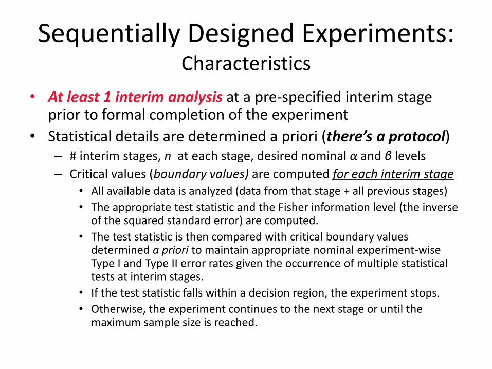
Sequentially Designed Experiments: Characteristics

• At least 1 interim analysis at a pre-specified interim stage prior to formal completion of the experiment

• Statistical details are determined a priori (there’s a protocol) – # interim stages, n at each stage, desired nominal α and β levels

– Critical values (boundary values) are computed for each interim stage • All available data is analyzed (data from that stage + all previous stages)

• The appropriate test statistic and the Fisher information level (the inverse of the squared standard error) are computed.

• The test statistic is then compared with critical boundary values determined a priori to maintain appropriate nominal experiment-wise Type I and Type II error rates given the occurrence of multiple statistical tests at interim stages.

• If the test statistic falls within a decision region, the experiment stops.

• Otherwise, the experiment continues to the next stage or until the maximum sample size is reached.

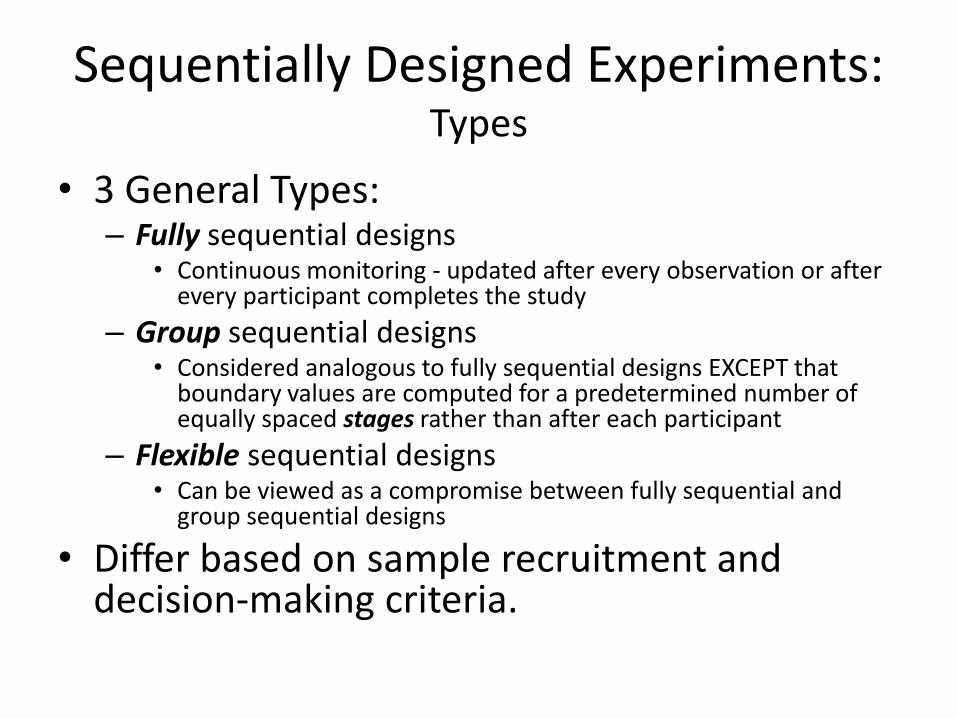
Sequentially Designed Experiments: Types

• 3 General Types: – Fully sequential designs

• Continuous monitoring - updated after every observation or after every participant completes the study

– Group sequential designs • Considered analogous to fully sequential designs EXCEPT that

boundary values are computed for a predetermined number of equally spaced stages rather than after each participant

– Flexible sequential designs • Can be viewed as a compromise between fully sequential and

group sequential designs

• Differ based on sample recruitment and decision-making criteria.

Sequentially Designed Experiments: Empirical Example

• CBC in the Early Grades (Sheridan et al, 2011) • 4-cohort fixed-design cluster randomized trial to

evaluate the effectiveness of a school-based consultation (CBC) approach for students with challenging classroom behaviors – 22 schools, 90 classrooms/teachers, 270 K-3rd grade

students & parents – Randomly assigned as small (2-3) parent-teacher groups to:

• business-as-usual control condition • experimental CBC condition.

• Study designed to detect a medium standardized effect (ES = .38).

Sequentially Designed Experiments: Methodological Study

• Bovaird et al, 2009; Bovaird, 2010 • Procedures

– Implemented a post hoc application of a sequential design and analysis strategy

– Cohort (4) = “Group”

– Assuming eventual “known” fixed design conclusions as true…

• What is the degree to which sample size savings may have been realized if we had implemented a group sequential design rather than a fixed design?

Sequentially Designed Experiments: Sequential vs. Fixed Design Results

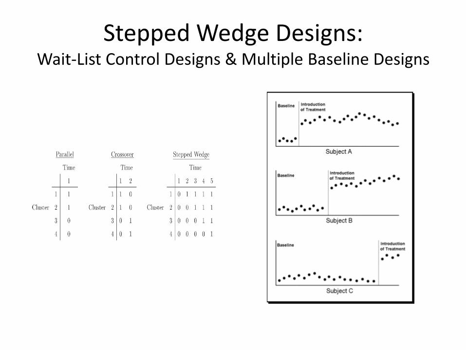
Stepped Wedge Designs: Wait-List Control Designs & Multiple Baseline Designs

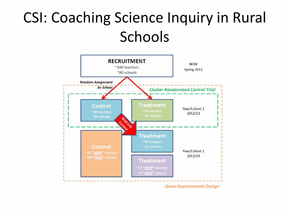
CSI: Coaching Science Inquiry in Rural Schools

CSI: Data Analysis

• The sample size is considered fixed and is determined by the maximum capacity of participating teachers in the treatment condition during a given year. This capacity is fixed at 50 treatment teachers per cohort. – The number of schools is the important sample size in terms of

statistical power.

• Traditional evaluation of the Cluster RCT via MLM/HLM • Re‐evaluation of the full 2‐year data set as a

quasi‐experimental Stepped-Wedge design • Re‐evaluation of the full 2‐year dataset as a

quasi‐experimental design with propensity score matching.

More-Efficient Measurement

Planned Missing Data Designs (PMDDs)

• “Efficiency-of-measurement design” (Graham, Taylor, Olchowski, & Cumsille, 2006) – Random sampling

– Optimal Designs

• See Allison, Allison, Faith, Paultre, & Pi-Sunyer (1997)

• Balance cost ($) with statistical power

– Fractional Factorial Designs

• See Box, Hunter, & Hunter (2005)

• Carefully chosen subset of cells from a factorial design focus “information” on most important conditions while minimizing resources

– Not so different from adaptive testing…

– Measurement Models

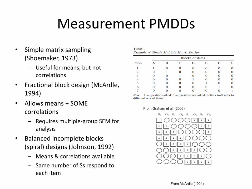
Measurement PMDDs

• Simple matrix sampling (Shoemaker, 1973)

– Useful for means, but not correlations

• Fractional block design (McArdle, 1994)

• Allows means + SOME correlations

– Requires multiple-group SEM for analysis

• Balanced incomplete blocks (spiral) designs (Johnson, 1992)

– Means & correlations available

– Same number of Ss respond to each item

From McArdle (1994)

From Graham et al. (2006)

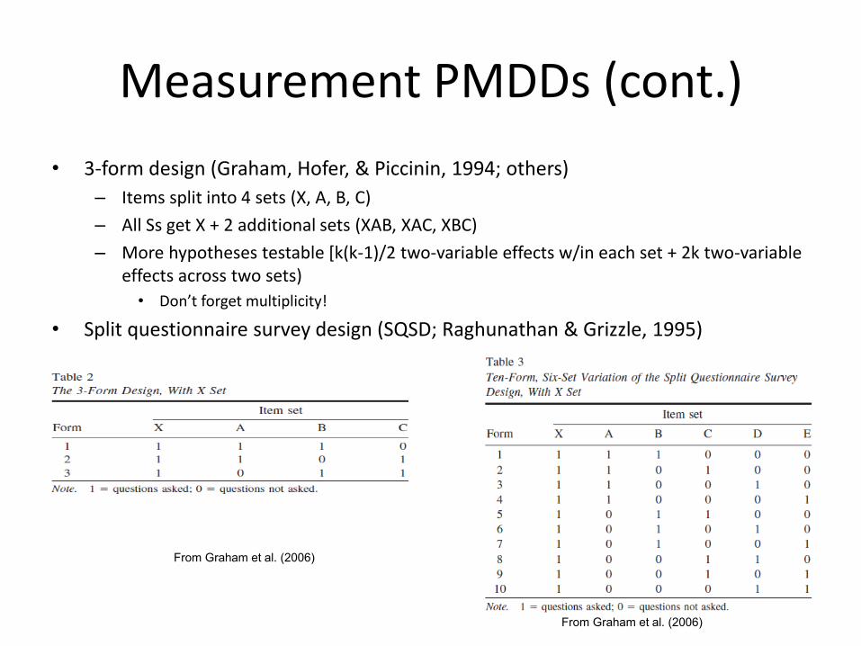
Measurement PMDDs (cont.)

• 3-form design (Graham, Hofer, & Piccinin, 1994; others)

– Items split into 4 sets (X, A, B, C)

– All Ss get X + 2 additional sets (XAB, XAC, XBC)

– More hypotheses testable [k(k-1)/2 two-variable effects w/in each set + 2k two-variable effects across two sets)

• Don’t forget multiplicity!

• Split questionnaire survey design (SQSD; Raghunathan & Grizzle, 1995)

From Graham et al. (2006)

From Graham et al. (2006)

Measurement PMDDs (cont.)

• 2-method measurement – Many cases w/ cheap, relatively noisy (lower reliability) measure

• i.e. self-report

• May require a response bias correction model

– Few cases w/ both cheap and expensive, more reliable measure

• i.e. biological markers

From Graham et al. (2006)

Accelerated Longitudinal Designs

• Convergence design

– Bell (1953)

• Cross-sequential design

– Schaie (1965)

• Cohort-sequential design

– Nesselroade & Baltes (1979)

• Accelerated longitudinal design

– Tonry, Ohlin, & Farrington (1991)

What Does Accelerated Mean?

• Overlapping ‘Cohorts’

– A cohort is a group of participants that begin a study at a common age or grade in school

• Tracked for a limited number of measurement occasions

• Groups are linked at their overlapping time points to approximate the true longitudinal curve/trajectory

GK G1 G2

Time 1 Time 2 Time 3

G1

G2 G3

Time 1 Time 2 Time 3

G2 G3 G4

Time 1 Time 2 Time 3

Cohort 1

Cohort 2

Cohort 3

Accelerated Longitudinal Design

• Advantages

– Allows for assessment of intra-individual change

– Takes less time than a purely longitudinal design

– Subject attrition and cumulative testing effects are not as prevalent

• Possible applications

– Any longitudinal research setting • Developmental research

• Educational or Classroom studies

• Gerontology or aging research

Small Samples but Big Models

Structural Equation Modeling

• A collection of techniques – Allow relationships between:

• 1 or more IVs (continuous or discrete) • One or more DVs (continuous or discrete)

– IVs & DVs can be either measured variables or latent constructs

• Construct: term often used to refer to some attribute we want to measure – In social sciences, most constructs are latent (i.e.,

unobservable) traits – How do you impart clear meaning to scores that measure

an unobservable trait? – Measurement instruments cannot exactly represent the

attributes we seek to measure

Structural Equation Modeling 4 Common Types of SEM Models

Structural Equation Modeling Research Questions

• Model Quality – Does the model fit the data? Does the model produce an estimated population

covariance matrix that is consistent with the sample (observed) covariance matrix? – Which theory (model) produces an estimated population covariance matrix that is most

consistent with the sample covariance matrix?

• Model Parameters

– How much variance in the DV(s) is accounted for by the IV(s)? – What is the value of the path coefficient? Is it significantly different from zero? Which

paths are more/less important? – Does an IV directly affect a specific DV or does the IV affect the DV through an

intermediary, or mediating, variable?

• Special Models

– Do two or more groups differ in the covariance matrices, regression coefficients, or means?

– Does a variable change over time? What is the shape of the change? Do individuals vary in their initial level or rate of change?

– How reliable are each of the measured variables?

Alternatives to SEM: Factor Analysis

• Exploratory – Principal components analysis (PCA)

– Parceling

– Obtain factor scores for higher order constructs

• Confirmatory – Model fit

• Larger # items = higher power w/ smaller N’s

– Parameter significance • Larger # items = lower power w/ smaller N’s

– Parameter precision • Smaller SE’s are easier to obtain by increasing the sample

size rather than reducing variability

Alternatives to SEM: Factor Scores

• Add (or average) variables together that load highly on a factor – variables with large SDs contribute more heavily to the solution – standardize first – in many cases, this will be adequate – Recommended in small samples

• Regression approach – Capitalizes on chance relationships, so factor-scores are biased – Often correlations among scores for factors even if supposed to be orthogonal – Best overall non-Bayesian method

• Bartlett method – Factor scores only correlate with their own factors & scores are unbiased – Factor scores may still be correlated with each other even when “orthogonal”

• Anderson-Rubin approach – Uncorrelated factor scores even if factors are correlated – Best if goal is an orthogonal score

• Empirical Bayes Estimation – Implemented in SEM & MLM programs – Ideal approach, but can suffer from shrinkage in small samples

Alternatives to SEM: Others

• Unweighted (ordinary) Least squares

• Reduce to path analysis

– Create summary score for each construct • PCA vs. FA vs. avg/sum of z-scores

– Analyze as ML with a reduced model

– Analyze with ULS/OLS as a multi-step regression

• Canonical correlation

• ML w/ Re-sampling procedures

– Use bootstrapping to obtain empirical standard errors

Re-sampling Methods

• Use the obtained data to generate a simulated population distribution – Resample hundreds/thousands of times – Defines an empirical sampling distribution – Distributional assumptions are now irrelevant – Validity

• internal – random sampling from the population is not necessary • external – random sampling is essential

• Uses: – Traditional hypothesis testing – Defining confidence intervals – Computing estimate stability – Measure estimate bias

• Types: – Randomization tests, Jackknife, Bootstrapping

Partial Least Squares PLS; Wold (1966, 1973, 1982)

• Uses fixed point (FP) algorithm for parameter estimation – Model parameters divided into subsets – Each set is partially estimated w/ OLS with other subset fixed – Switch & cycled through until convergence

• Avoids improper solutions by replacing factors w/ linear

composites of observed variables like in PCA • Does not rely on distributional assumptions

• Does not solve global optimization problem

– No single criterion consistently minimized/maximized to determine model parameter estimates (i.e. fit function in SEM)

– Difficult to evaluate PLS procedure – No mechanism to evaluate the overall goodness of fit

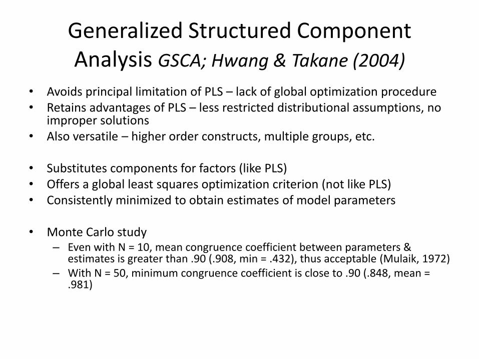
Generalized Structured Component Analysis GSCA; Hwang & Takane (2004)

• Avoids principal limitation of PLS – lack of global optimization procedure • Retains advantages of PLS – less restricted distributional assumptions, no

improper solutions • Also versatile – higher order constructs, multiple groups, etc.

• Substitutes components for factors (like PLS) • Offers a global least squares optimization criterion (not like PLS) • Consistently minimized to obtain estimates of model parameters

• Monte Carlo study

– Even with N = 10, mean congruence coefficient between parameters & estimates is greater than .90 (.908, min = .432), thus acceptable (Mulaik, 1972)

– With N = 50, minimum congruence coefficient is close to .90 (.848, mean = .981)

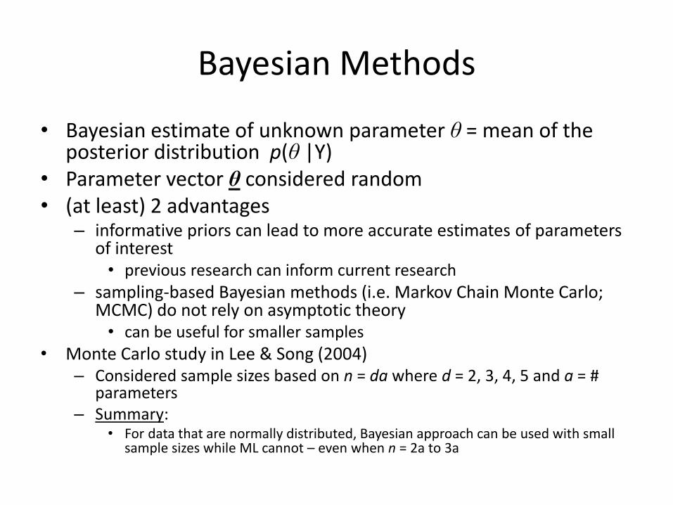
Bayesian Methods

• Bayesian estimate of unknown parameter θ = mean of the posterior distribution p(θ |Y)

• Parameter vector θ considered random • (at least) 2 advantages

– informative priors can lead to more accurate estimates of parameters of interest • previous research can inform current research

– sampling-based Bayesian methods (i.e. Markov Chain Monte Carlo; MCMC) do not rely on asymptotic theory • can be useful for smaller samples

• Monte Carlo study in Lee & Song (2004) – Considered sample sizes based on n = da where d = 2, 3, 4, 5 and a = #

parameters – Summary:

• For data that are normally distributed, Bayesian approach can be used with small sample sizes while ML cannot – even when n = 2a to 3a

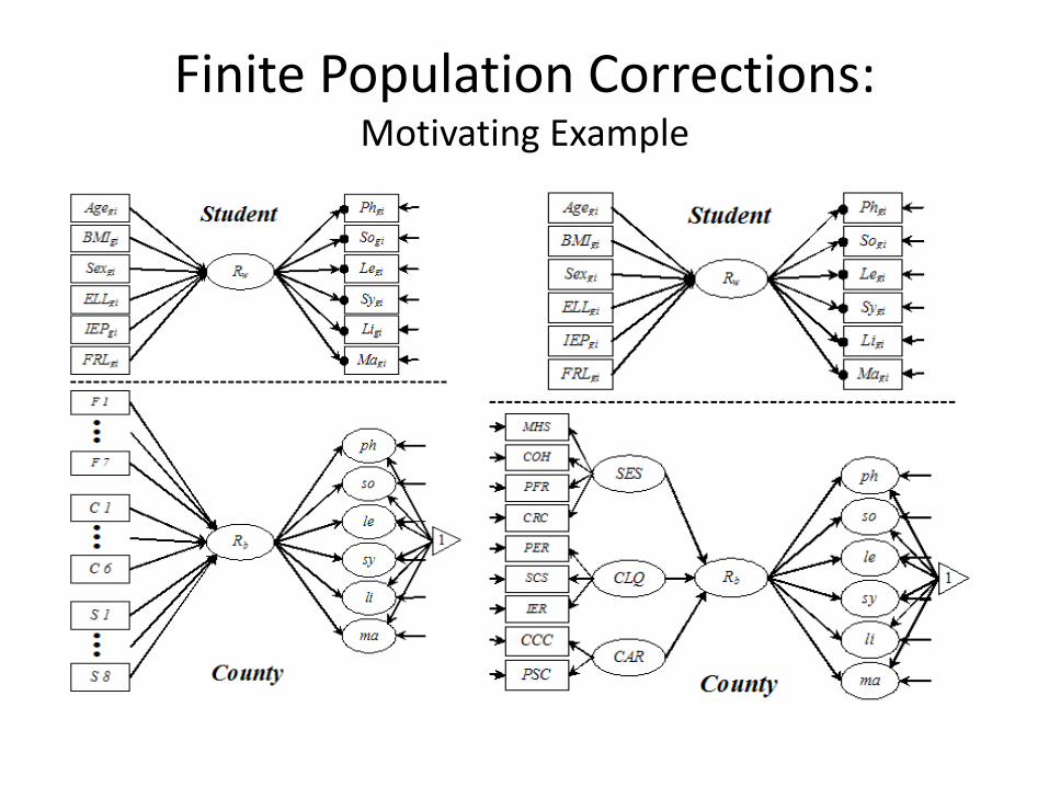
Finite Population Corrections: Motivating Example

Finite Population Corrections: Some Limiting Conditions?

• Problem(s) – Small N - but almost all of the available data

– Small effects – indirect/proxy effects

• Sampling in MLM – possible to obtain proportionally large samples or near-census

sampling at the macro-levels

– especially when sampling from finite geographical locations

• Relevance: – educational testing

– cross-cultural research

– behavioral ecosystems modeling

• Potential solution?? – finite population correction (fpc)

Finite Population Correction (fpc)

• Definition – Reduces sampling error by decreasing the variance related to the

sampling method (sampling without replacement)

– Adjustment factor varies with the sample size, and is directly related to the proportion of the population sampled

• Usefulness – When finite population corrections are omitted, the standard errors

are overestimated

– Standard formulas assume sample taken from a population so large that it may as well be infinite

– The fpc factors may be used to develop confidence estimates or in sample size estimation

Finite Population Correction (fpc)

• Guidelines for applying fpc – May be applied to either the variance or the standard

error • Formula for variance: (N-n) / (N-1) • Formula for standard error: √ ((N-n) / (N-1))

– Proportion of population that may be sampled without application of fpc depends on the research question and the size of effects expected

– When less than 5% of population has been sampled, fpc factor is negligible

– Proportion of population for which fpc should be applied is not completely agreed upon – generally 5% - 10%

Finite Population Corrections: Primary Model Results

Finite Population Corrections: Sub Model Results

Finite Population Corrections: Simple Regression vs. Multiple Regression

0.000

0.005

0.010

0.015

0.020

0.025

0.030

0.035

0.040

0.045

10 20 30 40 50 60 70 80 90

% Sampled (out of 100)

Sta

nd

ard

Err

or

0.494

0.495

0.496

0.497

0.498

0.499

Pa

ram

ete

r E

stim

ate

Pop. B

Mean B

Avg. B

Mean SE

Emp SE

SD B

fpc SE

Avg. SE

0.000

0.005

0.010

0.015

0.020

0.025

0.030

0.035

0.040

30 40 50 60 70 80 90

% Sampled (out of 100)

Sta

nd

ard

Err

or

-0.05

0.00

0.05

0.10

0.15

0.20

0.25

0.30

0.35

Pa

ram

ete

r E

stim

ate

Mean SE

SD B

fpc SE

Mean B

Finite Population Corrections: Relevance

• How realistic, or meaningful are finite samples?

– Very realistic for upper hierarchical levels in education • School districts (NCLB), counties (state ed. depts.), states

(NAEP/NCLB), countries (PISA)

– Moderately realistic for cross-cultural studies when assessing culture/country-level variables

– Potentially realistic for small clinical, under-represented, or geographically isolatable populations

The research reported here was supported by the Institute of Education Sciences, U.S. Department of Education, through Grant # R305C090022 to the University of Nebraska-Lincoln. The opinions expressed are

those of the authors and do not represent views of the Institute or the U.S. Department of Education.