The Fundamental Theorem of Derivative Tradingmt/pdfFiles/FToDT presentation.pdf · The Fundamental...
107
The Fundamental Theorem of Derivative Trading - Exposition, Extensions, and Experiments Martin J¨ onsson Visiting PhD Candidate, Mathematical Institute University of Oxford Department of Mathematical Sciences Mathematical and Statistical Methods in Insurance and Finance University of Copenhagen [email protected] [email protected] February 26, 2016
Transcript of The Fundamental Theorem of Derivative Tradingmt/pdfFiles/FToDT presentation.pdf · The Fundamental...
The Fundamental Theorem of Derivative Trading- Exposition, Extensions, and Experiments
Martin JonssonVisiting PhD Candidate, Mathematical Institute
University of Oxford
Department of Mathematical SciencesMathematical and Statistical Methods in Insurance and Finance
University of Copenhagen
February 26, 2016
Joint work with Simon Ellersgaard and Rolf Poulsen, University of Copenhagen.Based on paper with the same title, to appear in Quantitative Finance.
The Fundamental Theorem of Derivative Trading 2/45

Introduction
The Fundamental Theorem of Derivative Trading 3/45

Introduction
The issue of model uncertainty in the context of derivative hedging
I The art of derivative hedging undoubtedly lies at the heart ofmathematical finance.
I Hedging in real-world practice is, however, a challenging issue: even witha perfect model for the underlying, we still need exact inference for amodel-based hedging strategy to be successful.
I Assuming the standard SDE paradigm for the financial market, the issueemanates from the latent nature of volatility.
I We can only hope for a measured quantity: historical volatility fromlog-returns or implied volatility from observed option prices
The Fundamental Theorem of Derivative Trading 4/45
Introduction
I Measuring Historical Volatility suffers from the usual challenges ofstatistical inference: we need a never ending time series of historicalreturns.
I Reversing Implied Volatility from market option prices might beill-defined...
I ...and it is hard to believe that the market hysteria which drives the pricesof traded options shall capture the market hysteria that drives the pricesof the underlying asset.
The Fundamental Theorem of Derivative Trading 5/45

Introduction
I Studies into robustness of the delta-hedge appear in Karoui,Jeanblanc-Picque & Shreve (1998) with a simple result for theprofit-and-loss of a hedge portfolio under misspecified volatility.
I The result, as we call The Fundamental Theorem of Derivate Trading,will be the usual suspect for our study:
I We derive a more general version, discuss various corollaries andextensions, and test some of its applications in an empirical context.
The Fundamental Theorem of Derivative Trading 6/45
Introduction
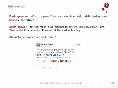
Basic question: What happens if we use a simple model to delta-hedge somefinancial derivative?
Short answer: Not too much if we manage to get the volatility about right.That is the Fundamental Theorem of Derivative Trading.
About to become a text-book result?
The Fundamental Theorem of Derivative Trading 7/45
Introduction
Basic question: What happens if we use a simple model to delta-hedge somefinancial derivative?
Short answer: Not too much if we manage to get the volatility about right.That is the Fundamental Theorem of Derivative Trading.
About to become a text-book result?
The Fundamental Theorem of Derivative Trading 7/45
Assumptions
The Fundamental Theorem of Derivative Trading 8/45
Assumptions
The set-up
I P-dynamics: Objective model for the underlying ”real-world” financialmarket.
I Mi -pricing: Option-pricing model assumed to represent collective optionmarket.
I Mh-hedging: Hedging model used for our personal purposes.
We do not assume a connection between the three models: the objective modelis fixed, the option model is implied by the option market and the hedgingmodel is our personal choice.
The Fundamental Theorem of Derivative Trading 9/45
Assumptions
The real-world financial market model
On a complete, filtered probability space (Ω,F ,F,P), the price processes of ndividend-paying risky assets X t = (X1t , ...,Xnt)
> following
dX t = DX t [µr (t, X t)dt + σr (t, X t)dW t ],
where DX t = diag(X1t , ...,Xnt), and W t is a n-dimensional Brownian motion.The coefficients µr (·, ·) and σr (·, ·) are assumed sufficiently well-behaved forthe SDE to have a unique solution.
X t is defined as the vector (X t ;χt) where χt is a state variable following somedynamics which are irrelevant to what follows.
A money account with price process Bt govern by
dBt = rtBtdt
where rt = r(t,X t) is the locally risk-free rate.
The Fundamental Theorem of Derivative Trading 10/45
Assumptions
The real-world financial market modelOn a complete, filtered probability space (Ω,F ,F,P), the price processes of ndividend-paying risky assets X t = (X1t , ...,Xnt)
> following
dX t = DX t [µr (t, X t)dt + σr (t, X t)dW t ],
where DX t = diag(X1t , ...,Xnt), and W t is a n-dimensional Brownian motion.The coefficients µr (·, ·) and σr (·, ·) are assumed sufficiently well-behaved forthe SDE to have a unique solution.
X t is defined as the vector (X t ;χt) where χt is a state variable following somedynamics which are irrelevant to what follows.
A money account with price process Bt govern by
dBt = rtBtdt
where rt = r(t,X t) is the locally risk-free rate.
The Fundamental Theorem of Derivative Trading 10/45
Assumptions
The Hedging model: our personal perspective
We are completely unaware (or ignorant) of the true form of the real modelµr (·, ·), σr (·, ·) and the existence of χt . Instead, we assume the asset price tofollow a local volatility model (under our pricing measure) represented by adeterministic diffusion function in Rn×n
Mh : σh(t, x).
Mh corresponds to the belief that a European options have a Markovianpricing rule V h
t = V h(t,X t) where V h(t, x) is a deterministic C1,2-functionsatisfying Black-Scholes equation
rtVh = ∂tV
h +∇xVh • ((rt1− qt) x) +
1
2tr[σᵀ
hDx∇2xxV
hDxσh],
V h(T , x) = g(x),
where qt = q(t, x) is the vector of yield rates, • the dot product, theHadamard product, tr[·] the trace operator and ∇x , ∇2
xx the gradient- andHessian operator.
The Fundamental Theorem of Derivative Trading 11/45
Assumptions
The Hedging model: our personal perspectiveWe are completely unaware (or ignorant) of the true form of the real modelµr (·, ·), σr (·, ·) and the existence of χt . Instead, we assume the asset price tofollow a local volatility model (under our pricing measure) represented by adeterministic diffusion function in Rn×n
Mh : σh(t, x).
Mh corresponds to the belief that a European options have a Markovianpricing rule V h
t = V h(t,X t) where V h(t, x) is a deterministic C1,2-functionsatisfying Black-Scholes equation
rtVh = ∂tV
h +∇xVh • ((rt1− qt) x) +
1
2tr[σᵀ
hDx∇2xxV
hDxσh],
V h(T , x) = g(x),
where qt = q(t, x) is the vector of yield rates, • the dot product, theHadamard product, tr[·] the trace operator and ∇x , ∇2
xx the gradient- andHessian operator.
The Fundamental Theorem of Derivative Trading 11/45
Assumptions
The Option-market model
We make the same assumptions on the structure of the pricing model thatrepresents the option market: a European option on X t has a market priceprocess V i
t = V i (t,X t) where V i (t, x) satisfies Black-Scholes equation with alocal volatility function in Rn×n
Mi : σi (t, x).
The local volatility model is consistent with observed market prices: for anobserved set of maturity-T strike-K put/call prices, V i (t,X t ;T ,K) matchesthe market for every (T ,K) and state (t,X t) of the underlying.
The Fundamental Theorem of Derivative Trading 12/45
Assumptions
The Option-market modelWe make the same assumptions on the structure of the pricing model thatrepresents the option market: a European option on X t has a market priceprocess V i
t = V i (t,X t) where V i (t, x) satisfies Black-Scholes equation with alocal volatility function in Rn×n
Mi : σi (t, x).
The local volatility model is consistent with observed market prices: for anobserved set of maturity-T strike-K put/call prices, V i (t,X t ;T ,K) matchesthe market for every (T ,K) and state (t,X t) of the underlying.
The Fundamental Theorem of Derivative Trading 12/45
Assumptions
Remark. The objective model for the financial market (Bt ,X t) is aprobabilistic model, while Mh and Mi correspond to pricing rules V h(t, x),V i (t, x) being deterministic functions. In this context, Mh and Mi are notprobabilistic models per se, although traditionally derived from a probabilisticdescription of the underlying.
The Fundamental Theorem of Derivative Trading 13/45

The Theorem
The Fundamental Theorem of Derivative Trading 14/45
The Theorem
We now consider what happens in following the scenario:
I The asset prices X t follow the real P-dynamics.
I We employ Mh for hedging a European option written on X t , which webuy at time t = 0.
I The option is acquired on the option market, i.e. it has a value processgiven by V i
t = V i (t,X t), t ∈ [0,T ] and we pay V i0 for the option.
I We set out to ∆-hedge the option based on our personal hedging modelMh, which yields the fair price V h
0 at time t = 0, and furthermore, ahedge position ∆h
t ≡ ∇xVh(t,X t) at time t ∈ [0,T ].
I We hold the hedge-portfolio over the entire life-time of the option [0,T ].
The Fundamental Theorem of Derivative Trading 15/45
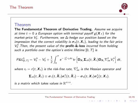
The Theorem
TheoremThe Fundamental Theorem of Derivative Trading. Assume we acquireat time t = 0 a European option with terminal payoff g(XT ) for themarket-price V i
0 . Furthermore, we ∆-hedge our position based on theimpression that the correct volatility is σh(t,X t), leading to the fair priceV h
0 .Then, the present value of the profit-&-loss incurred from holdingsuch a portfolio over the option’s entire lifetime [0,T ] is
P&Lh[0,T ] = V h
0 − V i0 +
1
2
∫ T
0
e−∫ t
0 rudu tr[DX t Σrh(t, X t)DX t∇
2xxV
ht
]dt,
where rt = r(t,X t) is the risk-free rate, ∇2xx is the Hessian operator and
Σrh(t, X t) ≡ σr (t, X t)σᵀr (t, X t)− σh(t,X t)σ
ᵀh (t,X t).
is a matrix which takes values in Rn×n.
The Fundamental Theorem of Derivative Trading 16/45

The Theorem
Proof:
I Let Πt , t ∈ [0,T ], denote the value process of the hedge portfolio longone option with value V i
t and short ∆hkt = ∂xkV
h(t,X t) units of Xkt ,k = 1, . . . , n. That is, ∆h
t = ∇xVh(t,X t) is the vector of units in the
underlying X t , where X t follows the real dynamics.
I Suppose Bt is chosen such that the net value is zero due to continuousre-balancing: Πh
t = V it + Bt −∆h
t • X t = 0.
I From the self-financing condition and previous equation
dΠht = dV i
t + rtBtdt −∆ht • (dX t + qt X tdt)
= dV it −∆h
t • (dX t − (rt1− qt) X tdt)− rtVit dt.
(1)
I Next, apply Ito’s lemma to V ht = V h(t,X t) to obtain
dV ht =
(∂tV
ht +
1
2tr[σ>r (t, X t)D>X t
∇2xxV
ht DX tσr (t, X t)
])dt +∇xV
ht • dX t .
The Fundamental Theorem of Derivative Trading 17/45
The Theorem
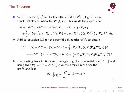
I Substitute for ∂tVht in the Ito differential of V h(t,X t) with the
Black-Scholes equation for V h(t, x). This yields the expression
0 = −dV ht + rtV
ht dt + ∆h
t • (dX t − (rt1− qt) X tdt)
+1
2tr[DX t
(σr (t, X t)σ
>r (t, X t)− σh(t,X t)σ
>h (t,X t)
)DX t∇
2xxV
ht
]dt.
I Add to equation (1) for the portfolio dynamics dΠht , to obtain
dΠht = dV i
t − dV ht − rt(V
it − V h
t )dt +1
2tr[DX t Σrh(t, X t)DX t∇
2xxV
ht ]dt
= e∫ t
0 rudud(e−
∫ t0 rudu(V i
t − V ht ))
+1
2tr[DX t Σrh(t, X t)DX t∇
2xxV
ht ]dt
I Discounting back to time zero, integrating the differential over [0,T ] andusing that V i
T = V hT = g(XT ) give the desired result for the
profit-and-loss
P&Lh[0,T ] ≡
∫ T
0
e−∫ t
0 rudtdΠht .
The Fundamental Theorem of Derivative Trading 18/45
The Theorem
Remarks
I The proof is a careful application of Ito’s lemma and the Black-Scholespricing equation. The important point is that our hedging model isassumed to be a local volatility model.
I The result is a generalization of the work by Karoui, Jeanblanc-Picque &Shreve (1998) (who viewed the result as negative since it proves nobounds for the error), as well as Ahmad & Wilmott (2005).
I The moniker The Fundamental Theorem of Derivative Trading wascoined (we think) by Andreasen (2003).
The Fundamental Theorem of Derivative Trading 19/45

The Theorem
Remarks
I The theorem can be extended in various directions: e.g. ifVt = V (t,Xt ,At) is the price of an Asian option on the continuousaverage At and underlying Xt , the the theorem remains form-invariant.
I The incorporation of jumps to the models is rather straightforward. Wewill consider this dynamical modification in the following.
I Further, for the profit-and-loss formula, we note that the option marketprice enters only through the initial price V i
0 . This is because we look atthe accrued profit throughout the entire life-time [0,T ]. We willelaborate on the mark-to-market situation in the coming.
I Clearly, the profit-and-loss changes sign if we consider the situation wherewe go short the option, long the underlying.
The Fundamental Theorem of Derivative Trading 20/45
Corollaries
The Fundamental Theorem of Derivative Trading 21/45

Corollaries
I The Real Hedge:
If we perfectly match the real dynamics in our∆-hedge; σh(t,X t) = σr (t, X t) a.s. for all t ∈ [0,T ], then our terminalprofit-and-loss is deterministic
P&Lh=r[0,T ] = V r
0 − V i0
provided we hold the hedge portfolio until maturity (and hedgecontinuously in time).
I However, day-to-day fluctuations of the hedge portfolio still evolveserratically:
dΠh=rt =
1
2tr[DX t Σri (t, X t)DX t∇
2xxV
it ]dt
+∇x(V it − V r
t ) •
(µrt − rt1 + qt) X tdt + DX tσr (t, X t)dW t
.
I That is, the mark-to-market P&L dynamics is driven by a dW t-term (theeffect of which is clearly visible when hedging with discrete, dailyrebalancing).
The Fundamental Theorem of Derivative Trading 22/45
Corollaries
I The Real Hedge: If we perfectly match the real dynamics in our∆-hedge; σh(t,X t) = σr (t, X t) a.s. for all t ∈ [0,T ], then our terminalprofit-and-loss is deterministic
P&Lh=r[0,T ] = V r
0 − V i0
provided we hold the hedge portfolio until maturity (and hedgecontinuously in time).
I However, day-to-day fluctuations of the hedge portfolio still evolveserratically:
dΠh=rt =
1
2tr[DX t Σri (t, X t)DX t∇
2xxV
it ]dt
+∇x(V it − V r
t ) •
(µrt − rt1 + qt) X tdt + DX tσr (t, X t)dW t
.
I That is, the mark-to-market P&L dynamics is driven by a dW t-term (theeffect of which is clearly visible when hedging with discrete, dailyrebalancing).
The Fundamental Theorem of Derivative Trading 22/45
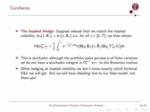
Corollaries
I The Implied Hedge:
Suppose instead that we match the impliedvolatility; σh(t,X t) = σi (t,X t) a.s. for all t ∈ [0,T ], we then obtain
P&Lh=i[0,T ] =
1
2
∫ T
0
e−∫ t
0 rudutr[DX t Σri (t, X t)DX t∇2xxV
it ]dt.
I This is stochastic although the portfolio value process is of finite variation:we do not have a stochastic integral in Πh=i
t w.r. to the Brownian motion.
I When hedging at implied volatility we don’t know exactly which terminalP&L we will get. But we will have bleeding due to our false model, notblow-ups!
The Fundamental Theorem of Derivative Trading 23/45
Corollaries
I The Implied Hedge: Suppose instead that we match the impliedvolatility; σh(t,X t) = σi (t,X t) a.s. for all t ∈ [0,T ], we then obtain
P&Lh=i[0,T ] =
1
2
∫ T
0
e−∫ t
0 rudutr[DX t Σri (t, X t)DX t∇2xxV
it ]dt.
I This is stochastic although the portfolio value process is of finite variation:we do not have a stochastic integral in Πh=i
t w.r. to the Brownian motion.
I When hedging at implied volatility we don’t know exactly which terminalP&L we will get. But we will have bleeding due to our false model, notblow-ups!
The Fundamental Theorem of Derivative Trading 23/45

Corollaries
As for profitability
I The real hedge gives P&L = V r0 − V i
0 (provided continuous hedging): wesimply go short the hedge portfolio if V r
0 < V i0 to make a certain profit.
I The implied hedge: P&L = 12
∫ T0 e−
∫ t0 rudutr[DX t Σri (t, X t)DX t∇2
xxVit ]dt. By
property of the trace operator, we may write
tr[DX t Σri (t, X t)DX t∇2xxV
it ] = X>t (Σri (t, X t) ∇2
xxVit )X t
and we see that the P&L is positive (a.s.) if Σri (t, X t) ∇2xxV
it is a
positive definite matrix at all times (a.s.). By the Schur product theorem,this is the case if Σri (t, X t) and ∇2
xxVit are both positive definite matrices
individually.
The Fundamental Theorem of Derivative Trading 24/45
Corollaries
I Hedging with real volatility; a deterministic terminal P&L but we getthere in an erratic way, or hedging with implied volatility; a stochasticterminal P&L, but we get there in a smooth way.
I For a demonstration of this point we run a simulation experiment basedon Wilmott and Ahmad (2005).
The Fundamental Theorem of Derivative Trading 25/45
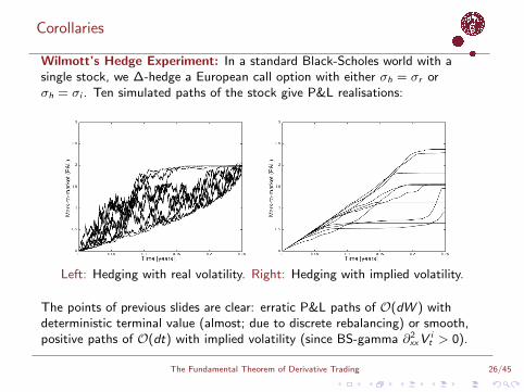
Corollaries
Wilmott’s Hedge Experiment: In a standard Black-Scholes world with asingle stock, we ∆-hedge a European call option with either σh = σr orσh = σi . Ten simulated paths of the stock give P&L realisations:
Left: Hedging with real volatility. Right: Hedging with implied volatility.
The points of previous slides are clear: erratic P&L paths of O(dW ) withdeterministic terminal value (almost; due to discrete rebalancing) or smooth,positive paths of O(dt) with implied volatility (since BS-gamma ∂2
xxVit > 0).
The Fundamental Theorem of Derivative Trading 26/45
Corollaries
Which Free Lunch Would You Like Today, Sir?
I Both strategies of the experiment simply suggest that if we know the realvolatility, e.g. from historical estimation σhist ≈ σr , and its relation to theimplied; σi < σhist (σi > σhist), then we can make a certain profit if we golong (short) the hedge portfolio.
I So, what happens if we run Wilmott’s experiment on market data; arethere any empirical support for these results?
The Fundamental Theorem of Derivative Trading 27/45
Experiments
The Fundamental Theorem of Derivative Trading 28/45

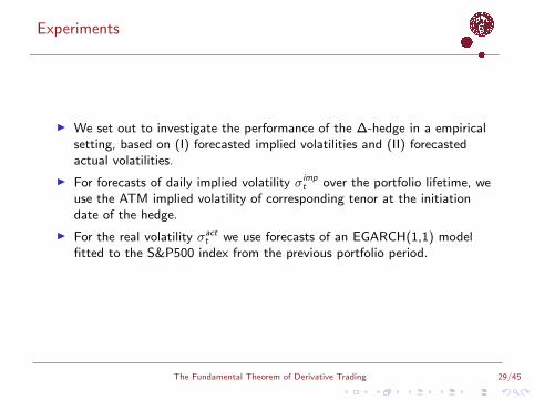
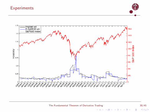
Experiments
I We set out to investigate the performance of the ∆-hedge in a empiricalsetting, based on (I) forecasted implied volatilities and (II) forecastedactual volatilities.
I For forecasts of daily implied volatility σimpt over the portfolio lifetime, we
use the ATM implied volatility of corresponding tenor at the initiationdate of the hedge.
I For the real volatility σactt we use forecasts of an EGARCH(1,1) model
fitted to the S&P500 index from the previous portfolio period.
The Fundamental Theorem of Derivative Trading 29/45
Experiments
The Fundamental Theorem of Derivative Trading 30/45
Experiments
I We investigate 36 hedge portfolios of three-month call options onS&P500, purchased at-the-money and kept until expiry.
I With daily rebalancing, we set up self-financing hedge portfolios based onthe Black-Scholes delta, long or short the call option depending on thesign of (σact
t − σimpt ), and we hold the portfolios until maturity.
The Fundamental Theorem of Derivative Trading 31/45
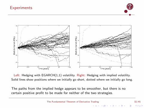
Experiments
Left: Hedging with EGARCH(1,1) volatility. Right: Hedging with implied volatility.
Solid lines show positions where we initially go short, dotted where we initially go long.
The paths from the implied hedge appears to be smoother, but there is nocertain positive profit to be made for neither of the two strategies.
The Fundamental Theorem of Derivative Trading 32/45
Experiments
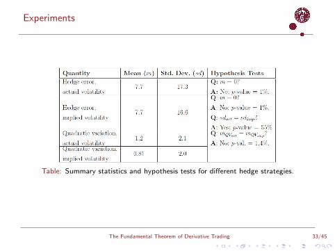
Table: Summary statistics and hypothesis tests for different hedge strategies.
The Fundamental Theorem of Derivative Trading 33/45

Experiments
I Although no certain positive terminal P&L for every path, we have asignificant positive payout on the average.
I If we are concerned about the terminal hedge error only: the strategiesyield equal mean and standard deviation, i.e. the strategies are notsignificantly different in riskiness.
I But when hedging with implied volatility, the quadratic variation of theP&L is more than halved compared to using actual volatility. This shouldmake you sleep better at night.
I At least we got one thing right: we may reduce the erratic behaviour ofour daily P&L-paths by hedging with the implied volatility. However, wecan not hope for a bang-on estimate of the real volatility; σh = σr , whichwould give P&L = V r
0 − V i0 . Neither can we hope for getting the sign
right of (σrt − σi
t), which would guarantee P&L paths positive attermination.
The Fundamental Theorem of Derivative Trading 34/45
Extensions: The Case of Jumps
The Fundamental Theorem of Derivative Trading 35/45
Extensions: The Case of Jumps
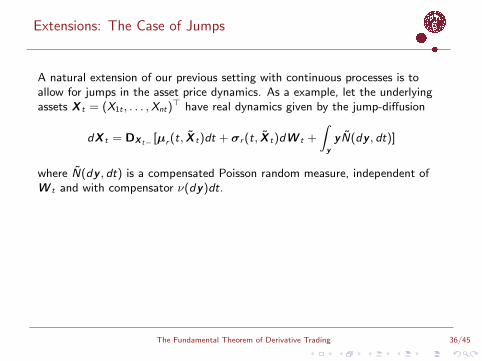
A natural extension of our previous setting with continuous processes is toallow for jumps in the asset price dynamics. As a example, let the underlyingassets X t = (X1t , . . . ,Xnt)
> have real dynamics given by the jump-diffusion
dX t = DX t− [µr (t, X t)dt + σr (t, X t)dW t +
∫yy N(dy , dt)]
where N(dy , dt) is a compensated Poisson random measure, independent ofW t and with compensator ν(dy)dt.
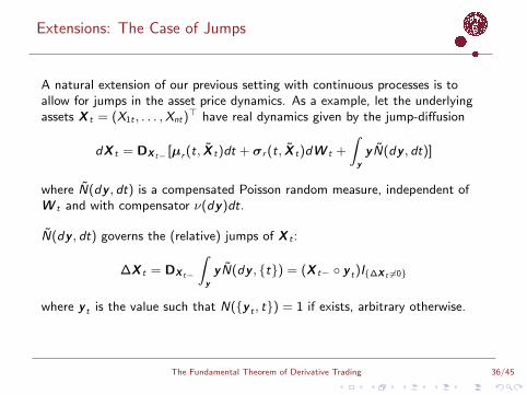
N(dy , dt) governs the (relative) jumps of X t :
∆X t = DX t−
∫yy N(dy , t) = (X t− y t)I∆X t 6=0
where y t is the value such that N(y t , t) = 1 if exists, arbitrary otherwise.
The Fundamental Theorem of Derivative Trading 36/45
Extensions: The Case of Jumps
A natural extension of our previous setting with continuous processes is toallow for jumps in the asset price dynamics. As a example, let the underlyingassets X t = (X1t , . . . ,Xnt)
> have real dynamics given by the jump-diffusion
dX t = DX t− [µr (t, X t)dt + σr (t, X t)dW t +
∫yy N(dy , dt)]
where N(dy , dt) is a compensated Poisson random measure, independent ofW t and with compensator ν(dy)dt.
N(dy , dt) governs the (relative) jumps of X t :
∆X t = DX t−
∫yy N(dy , t) = (X t− y t)I∆X t 6=0
where y t is the value such that N(y t , t) = 1 if exists, arbitrary otherwise.
The Fundamental Theorem of Derivative Trading 36/45
Extensions: The Case of Jumps
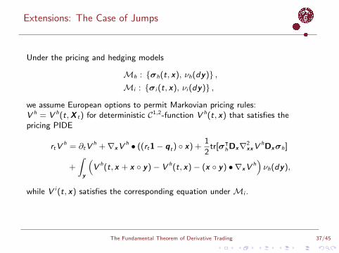
Under the pricing and hedging models
Mh : σh(t, x), νh(dy) ,Mi : σi (t, x), νi (dy) ,
we assume European options to permit Markovian pricing rules:V h = V h(t,X t) for deterministic C1,2-function V h(t, x) that satisfies thepricing PIDE
rtVh = ∂tV
h +∇xVh • ((rt1− qt) x) +
1
2tr[σᵀ
hDx∇2xxV
hDxσh]
+
∫y
(V h(t, x + x y)− V h(t, x)− (x y) • ∇xV
h)νh(dy),
while V i (t, x) satisfies the corresponding equation under Mi .
The Fundamental Theorem of Derivative Trading 37/45
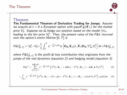
The Theorem
TheoremThe Fundamental Theorem of Derivative Trading for Jumps. Assumewe acquire at t = 0 a European option with payoff g(XT ) for the marketprice V i
0 . Suppose we ∆-hedge our position based on the model Mh,leading to the fair price V h
0 . Then, the present value of the P&L incurredover the option’s entire lifetime [0,T ] is
P&Lh[0,T ] = V h0 −V i
0+1
2
∫ T
0e−
∫ t0 rudu tr
[DX t Σrh(t, X t)DX t∇
2xxV
ht
]dt+P&LJ[0,T ]
where P&LJ[0,T ] is the profit-&-loss contribution that originates from the
jumps of the real dynamics (equation 2) and hedging model (equation 3)
P&LJ =
∆X t 6=0∑0≤t≤T
e−∫ t
0 rudu(V h(t,X t− + ∆X t )− V h(t,X t−)− ∆X t • ∇xV
h)
(2)
−∫
y,te−
∫ t0 rudu
(V h(t,X t− (1 + y))− V h(t,X t−)− (X t− y) • ∇xV
h)νh(dy)dt. (3)
The Fundamental Theorem of Derivative Trading 38/45
Extensions: The Case of Jumps
Remarks
I The proof: in a similar fashion as for the case without jumps but with thepricing PIDE and Ito’s lemma for a n-dimensional semimartingale.
I In fact, we may relax our assumptions to allow for the objective X t to bea general semimartingale and dropping the assumption on Mi as themarket price process V i
t t∈[0,T ] enters only through the initial value V i0 ,
provided we look at the case when hedging throughout [0,T ].
I The terminal hedge error decomposes into three parts originating from (I)the option’s model-to-market price difference, (II) the continuousquadratic variation of X t from the real- and hedging model, (III) thejumps ∆X t from the real dynamics and the hedging modeljump-distribution.
The Fundamental Theorem of Derivative Trading 39/45
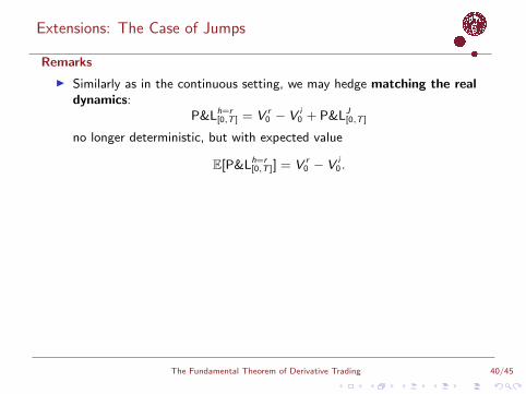
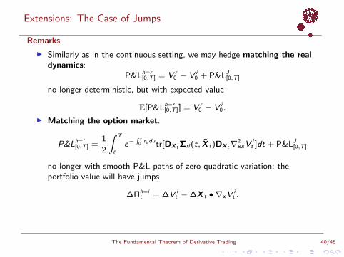
Extensions: The Case of Jumps
Remarks
I Similarly as in the continuous setting, we may hedge matching the realdynamics:
P&Lh=r[0,T ] = V r
0 − V i0 + P&LJ
[0,T ]
no longer deterministic, but with expected value
E[P&Lh=r[0,T ]] = V r
0 − V i0 .
I Matching the option market:
P&Lh=i[0,T ] =
1
2
∫ T
0
e−∫ t
0 rudutr[DX t Σri (t, X t)DX t∇2xxV
it ]dt + P&LJ
[0,T ]
no longer with smooth P&L paths of zero quadratic variation; theportfolio value will have jumps
∆Πh=it = ∆V i
t −∆X t • ∇xVit .
I One may argue that these points are in better agreement with outempirical results.
The Fundamental Theorem of Derivative Trading 40/45
Extensions: The Case of Jumps
Remarks
I Finally, if we consider the case where the pricing function V h(t, x) isconvex in x (e.g. plain vanilla puts and calls), we have that
∆X t 6=0∑0≤t≤T
e−∫ t
0 rudu(V h(t,X t− + ∆X t)− V h(t,X t−)−∆X t • ∇xV
h)
gives a positive contribution to the long-position P&L every time X t
jumps (in either direction). Conversely, for a short position, our hedgeportfolio takes a ”hit” every time a jump occurs: in Talebian termis, shortselling convex payoff options corresponds to...
The Fundamental Theorem of Derivative Trading 41/45
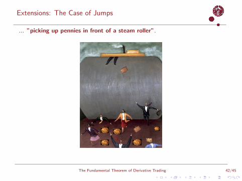
Extensions: The Case of Jumps
... ”picking up pennies in front of a steam roller”.
The Fundamental Theorem of Derivative Trading 42/45

Conclusion
The Fundamental Theorem of Derivative Trading 43/45
Conclusion
I We generalize the fundamental theorem of derivative trading, a result thatquantifies the profit-&-loss of a ∆-hedge under a misspecified volatility.
I We show that hedging with implied volatility yields smooth P&L pathswith changes of O(dt) while any other hedging volatility yields erraticpaths of O(dW ) (in the continuous setting: add jumps otherwise).
I We find empirical support for our theoretical results: there is evidencethat hedging at implied volatility does yield smoother P&L paths.
I However, the most conspicuous implication of the theorem – the easewith which arbitrage can be made if the relative sizes of σhist , σimp areknown – is not as convincing: even if we find a positive average, the P&Lmay readily turn negative.
I Finally, we extend the continuous models to affiliate jumps and may arguethat this setting better explains the results of our empirical investigation.
The Fundamental Theorem of Derivative Trading 44/45
Thank you for your attention!
For complete list of references, please see draft of our paper available at SSRN:
http://papers.ssrn.com/sol3/papers.cfm?abstract_id=2566425.
The Fundamental Theorem of Derivative Trading 45/45