The fundamental solution of compressible and ...

The fundamental solution of compressible andincompressible fluid flow past a rotating obstacle

JSPS-DFG Japanese-German Graduate ExternshipKickoff Meeting

Waseda University, Tokyo, June 17-18, 2014

Reinhard Farwig, TU DarmstadtMilan Pokorny, Charles University PragueToshiaki Hishida, Nagoya University, et al.

ω=|ω|(0,0,1)T

Ω

uoo

K

1 / 25

The fundamental solution of compressible andincompressible fluid flow past a rotating obstacle

JSPS-DFG Japanese-German Graduate ExternshipKickoff Meeting

Waseda University, Tokyo, June 17-18, 2014

Reinhard Farwig, TU DarmstadtMilan Pokorny, Charles University PragueToshiaki Hishida, Nagoya University, et al.

ω=|ω|(0,0,1)T

Ω

uoo

K1 / 25

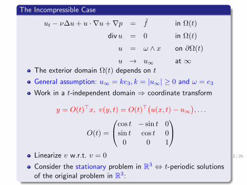
The Incompressible Case

ut − ν∆u+ u · ∇u+∇p = f in Ω(t)

divu = 0 in Ω(t)

u = ω ∧ x on ∂Ω(t)

u → u∞ at ∞The exterior domain Ω(t) depends on t

General assumption: u∞ = ke3, k = |u∞| ≥ 0 and ω = e3

Work in a t-independent domain ⇒ coordinate transform

y = O(t)>x, v(y, t) = O(t)>(u(x, t)− u∞

), . . .

O(t) =

cos t − sin t 0sin t cos t 0

0 0 1

Linearize v w.r.t. v = 0

Consider the stationary problem in R3 ⇔ t-periodic solutionsof the original problem in R3:

2 / 25

The Linear Problem

−ν∆v − (ω ∧ y) · ∇v + u∞ · ∇v + ω ∧ v +∇p = f in R3

div v = 0 in R3

v → 0 at ∞

• Apply the Helmholtz projection P ⇒Modified Stokes/Oseen operator

Aω,u∞(v) = −νP∆v − (ω ∧ y) · ∇v + ω ∧ v + u∞ · ∇v• T. Hishida (1999, 2000): Aω,u∞ does not (!) generate an

analytic semigroup

• Analysis of the fundamental solution in Lq-spaces:R. F., T. Hishida, D. Muller: Pacific J. Math. (2004)R. F.: Tohoku Math. J. (2005)G.P. Galdi, M. Kyed: Proc. Amer. Math. Soc. (2013), (2013)R. F., M. Krbec, S. Necasova: Ann. Univ. Ferrara (2008)R. F., M. Krbec, S. Necasova: Math. Methods Appl. Sci. (2008)

3 / 25

Further Literature

• Spectral properties of Aω,u∞ :R. F., J. Neustupa: Integral Equations Operator Theory (2008)R. F., S. Necasova, J. Neustupa: J. Math. Soc. Japan (2011)

• Explicit representation of the fundamental solution:R. F., R.B. Guenther, S. Necasova, E.A. Thomann: DCDS-A(2014)

• Semigroup estimates:M. Geissert, H. Heck, M. Hieber: J. reine angew. Math. (2006)T. Hishida, Y. Shibata: Arch. Ration. Mech. Anal. (2009)

• Numerous results on the nonlinear problem, e.g. byF.-Hishida, F.-Galdi-Kyed, Galdi-Kyed, Galdi-Silvestre,Geissert-Heck-Hieber, Goetze, Hansel, Heck-Kim-Kozono,Hieber-Shibata, Hieber-Sawada, Hishida-Shibata, et al.

4 / 25

Lq-estimates for the Fundamental Solution

Determine the fundamental solution, prove Lq-estimates

Use cylindrical coordinates y ∼ (r, θ, y3), r = |(y1, y2)| ≥ 0 ⇒(ω ∧ y) · ∇ = ∂θ

Use Fourier transform and cylindrical coordinatesξ ∼ (s, ϕ, ξ3) ⇒ ∂θu(ξ) = ∂ϕu(ξ) ⇒

We get a first order ODE w.r.t. ϕ:

ν|ξ|2v + ikξ3v − ∂ϕv + ω ∧ v = P f , iξ · v = 0,

where v has to be 2π-periodic in ϕ

5 / 25

Lq-estimates for the Fundamental Solution


Use cylindrical coordinates y ∼ (r, θ, y3), r = |(y1, y2)| ≥ 0 ⇒(ω ∧ y) · ∇ = ∂θ

Use Fourier transform and cylindrical coordinatesξ ∼ (s, ϕ, ξ3) ⇒ ∂θu(ξ) = ∂ϕu(ξ) ⇒We get a first order ODE w.r.t. ϕ:

ν|ξ|2v + ikξ3v − ∂ϕv + ω ∧ v = P f , iξ · v = 0,

where v has to be 2π-periodic in ϕ

5 / 25

The solution of the First Order ODE (ν = 1)

v(ξ) =1

1− e−2π|ξ|2∫ 2π

0e−|ξ|

2t−iktξ3O(t)>P f(O(t)ξ) dt

=

∫ ∞0

e−|ξ|2tO(t)>F((Pf)(O(t) · −kte3)) dt

If k = 0 and O(t)>((Pf)(O(t)·) is t-independent ⇒

v(ξ) = 1|ξ|2 P f(ξ) ⇒ ‖∇2v‖q ≤ c‖f‖q for 1 < q <∞

For q = 2: L2-estimates of ∇2v by Plancherel’s Theorem

Evidence that the integral kernel Γ satisfies

|Γ(x, y)| ≥ log |x− y||x− y|

6 / 25

Partition of Unity and Littlewood-Paley Theory (k = 0)

To control ∇2v ∼ ∆v let

ψ(ξ) = |ξ|2e−|ξ|2 , ψt(x) = t−n/2ψ( x√

t

), t > 0

Decompose ψ =∑

j χj ∗ ψ =:∑

j ψj

Use Littlewood-Paley theory for ‖ · ‖q:

‖f‖q ∼∥∥∥(∫ ∞

0|ϕs ∗ f(·)|2ds

s

)1/2∥∥∥q

Decompose operator

T : f 7→ ∆v(x) =

∫R3

K(x, y)Pf(y) dy,

into pieces Tj via ψj , i.e. T =∑Tj

7 / 25

Estimate of Tj (I)

‖Tjf‖q ≤ c2−|j|‖Mj‖1/2SL(L(q/2)′ )‖f‖q

where

Mjg(x) = supr>0

∫ 16r

r/16(|ψjt | ∗ |g|)(O(t)>x)

dt

t

Prove thatMjg(x) ≤ c2−2|j|M(Mθg)(x)

M is the classical Hardy-Littlewood maximal operator,bounded on Lq for each 1 < q <∞

8 / 25

Estimate of Tj (II)

(Mθg)(x) = supr>0

∫ 16r

r/16|g(O(t)>x|dt

t

behaves like a 1D maximal operator in θ for eachr = |(x1, x2)|, x3 and is bounded on Lq for each 1 < q <∞

End of Proof - Incompressible Case

‖Tjf‖q ≤ c2−2|j|‖f‖q ⇒ T is bounded on Lq, q ≥ 2

Complex interpolation ⇒ T is bounded on Lq, 1 < q <∞

9 / 25

The Compressible Case

Flow of a viscous, compressible fluid around (u∞ = 0) or past(0 6= u∞//e3) a rotating obstacle with angular velocityω = e3//u∞:

ρ∂u

∂t+ ρu · ∇u− µ∆u− (µ+ ν)∇divu+∇p(ρ) = ρf

∂ρ

∂t+ div (ρu) = 0

together with the boundary conditions

u(x, t) = ω ∧ x at⋃

t∈(0,∞)

∂Ω(t)× t

u(x, t)→ u∞ as |x| → ∞ρ(x, t)→ ρ∞ as |x| → ∞.

10 / 25

The new system (I) in v, σ

The exterior domain Ω(t) depends on t

Use a coordinate transform as before to work in at-independent domain:

y = O(t)>x, v(y, t) = O(t)>(u(x, t)− u∞

), ρ(y, t) = ρ(x, t)

Linearize v w.r.t. v = 0, linearize ρ w.r.t. to ρ∞ = 1 :ρ = 1 + σ

Consider the stationary problem in R3 ⇔ t-periodic solutionsof the original problem in R3

11 / 25

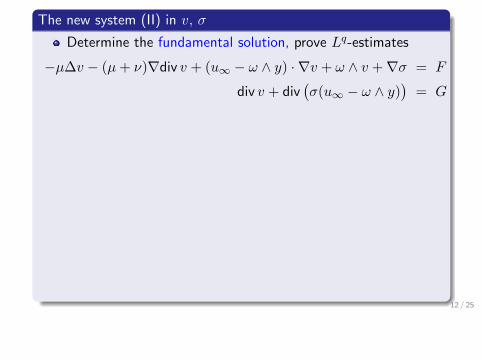
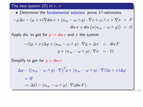
The new system (II) in v, σ


−µ∆v − (µ+ ν)∇div v + (u∞ − ω ∧ y) · ∇v + ω ∧ v +∇σ = F

div v + div(σ(u∞ − ω ∧ y)

)= G

Apply div to get for g := div v and σ the system

−(2µ+ ν)∆g + (u∞ − ω ∧ y) · ∇g + ∆σ = divF

g + (u∞ − ω ∧ y) · ∇σ = G.

Simplify to get for g = div v

∆g −((u∞ − ω ∧ y) · ∇

)2g + (u∞ − ω ∧ y) · ∇(2µ+ ν)∆g

= H

:= ∆G− (u∞ − ω ∧ y) · ∇(divF ).

12 / 25

The new system (II) in v, σ


−µ∆v − (µ+ ν)∇div v + (u∞ − ω ∧ y) · ∇v + ω ∧ v +∇σ = F

div v + div(σ(u∞ − ω ∧ y)

)= G

Apply div to get for g := div v and σ the system

−(2µ+ ν)∆g + (u∞ − ω ∧ y) · ∇g + ∆σ = divF

g + (u∞ − ω ∧ y) · ∇σ = G.

Simplify to get for g = div v

∆g −((u∞ − ω ∧ y) · ∇

)2g + (u∞ − ω ∧ y) · ∇(2µ+ ν)∆g

= H

:= ∆G− (u∞ − ω ∧ y) · ∇(divF ).12 / 25

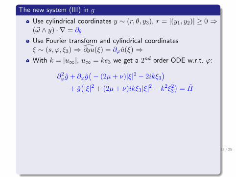
The new system (III) in g

Use cylindrical coordinates y ∼ (r, θ, y3), r = |(y1, y2)| ≥ 0 ⇒(~ω ∧ y) · ∇ = ∂θ

Use Fourier transform and cylindrical coordinatesξ ∼ (s, ϕ, ξ3) ⇒ ∂θu(ξ) = ∂ϕu(ξ) ⇒

With k = |u∞|, u∞ = ke3 we get a 2nd order ODE w.r.t. ϕ:

∂2ϕg + ∂ϕg(− (2µ+ ν)|ξ|2 − 2ikξ3

)+ g(|ξ|2 + (2µ+ ν)ikξ3|ξ|2 − k2ξ23

)= H

Characteristic polynomial

χ(λ) = λ2 −((2µ+ ν)|ξ|2 + 2ikξ3

)λ

+(|ξ|2 + (2µ+ ν)ikξ3|ξ|2 − k2ξ23

)Characteristic zeros

λ1,2(ξ) =1

2

((2µ+ ν)|ξ|2 + 2ikξ3 ±

√(2µ+ ν)2|ξ|4 − 4|ξ|2

).

13 / 25

The new system (III) in g

Use cylindrical coordinates y ∼ (r, θ, y3), r = |(y1, y2)| ≥ 0 ⇒(~ω ∧ y) · ∇ = ∂θ

Use Fourier transform and cylindrical coordinatesξ ∼ (s, ϕ, ξ3) ⇒ ∂θu(ξ) = ∂ϕu(ξ) ⇒With k = |u∞|, u∞ = ke3 we get a 2nd order ODE w.r.t. ϕ:

∂2ϕg + ∂ϕg(− (2µ+ ν)|ξ|2 − 2ikξ3

)+ g(|ξ|2 + (2µ+ ν)ikξ3|ξ|2 − k2ξ23

)= H

Characteristic polynomial

χ(λ) = λ2 −((2µ+ ν)|ξ|2 + 2ikξ3

)λ

+(|ξ|2 + (2µ+ ν)ikξ3|ξ|2 − k2ξ23

)Characteristic zeros

λ1,2(ξ) =1

2

((2µ+ ν)|ξ|2 + 2ikξ3 ±

√(2µ+ ν)2|ξ|4 − 4|ξ|2

).

13 / 25

The solution g

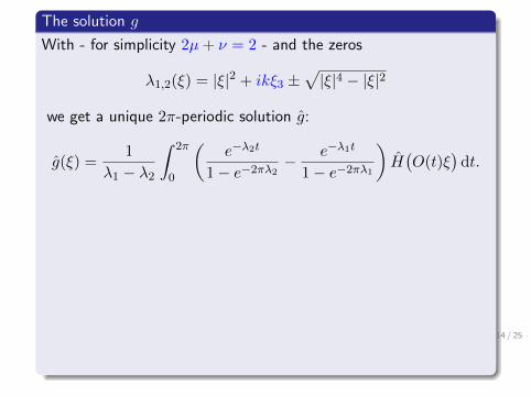
With - for simplicity 2µ+ ν = 2 - and the zeros

λ1,2(ξ) = |ξ|2 + ikξ3 ±√|ξ|4 − |ξ|2

we get a unique 2π-periodic solution g:

g(ξ) =1

λ1 − λ2

∫ 2π

0

(e−λ2t

1− e−2πλ2− e−λ1t

1− e−2πλ1

)H(O(t)ξ

)dt.

If H and H are independent of θ and φ, resp., then

g(ξ) = 2πH(ξ)(|ξ|2 + 2ikξ3|ξ|2 − k2ξ23

)−1.

We also have, with µ1,2(ξ) = |ξ|2 ±√|ξ|4 − |ξ|2,

g(ξ) =

∫ ∞0

e−µ2t − e−µ1t

µ1 − µ2F(H(O(t) · −kte3)

)(ξ) dt

14 / 25

The solution g

With - for simplicity 2µ+ ν = 2 - and the zeros

λ1,2(ξ) = |ξ|2 + ikξ3 ±√|ξ|4 − |ξ|2

we get a unique 2π-periodic solution g:

g(ξ) =1

λ1 − λ2

∫ 2π

0

(e−λ2t

1− e−2πλ2− e−λ1t

1− e−2πλ1

)H(O(t)ξ

)dt.

If H and H are independent of θ and φ, resp., then

g(ξ) = 2πH(ξ)(|ξ|2 + 2ikξ3|ξ|2 − k2ξ23

)−1.

We also have, with µ1,2(ξ) = |ξ|2 ±√|ξ|4 − |ξ|2,

g(ξ) =

∫ ∞0

e−µ2t − e−µ1t

µ1 − µ2F(H(O(t) · −kte3)

)(ξ) dt 14 / 25

Fourier Analysis

Note: µ1,2(ξ) is a smooth multiplier function on R3 \ 0 \ ∂B1

Use a partition of unity 1 = η0 + η1 + η2 where

η0 ∈ C∞0 (B1/2), η1(ξ) = 1 for1

2≤ |ξ| ≤ 2, η2 = 1 in (B4)

c

For |ξ| > 4 all multiplier functions are smooth, Hormander-Mikhlinmultiplier theory ⇒ Lq-estimates, 1 < q <∞For 0 < |ξ| < 1

4 all multiplier functions are smooth,Hormander-Mikhlin multiplier theory ⇒ Lq-estimates, 1 < q <∞Analysis near |ξ| = 1: multiplication of smooth multiplierfunctions (okay) with the crucial multiplier functions

η1(ξ)√

1− |ξ|2χB1(ξ) ∼ (1− |ξ|2)1/2+ ,

η1(ξ)√|ξ|2 − 1χBc

1(ξ) ∼ η1(ξ)(|ξ|2 − 1|)1/2+

15 / 25

Fourier Analysis



η0 ∈ C∞0 (B1/2), η1(ξ) = 1 for1

2≤ |ξ| ≤ 2, η2 = 1 in (B4)

c

For |ξ| > 4 all multiplier functions are smooth, Hormander-Mikhlinmultiplier theory ⇒ Lq-estimates, 1 < q <∞

For 0 < |ξ| < 14 all multiplier functions are smooth,

Hormander-Mikhlin multiplier theory ⇒ Lq-estimates, 1 < q <∞Analysis near |ξ| = 1: multiplication of smooth multiplierfunctions (okay) with the crucial multiplier functions

η1(ξ)√

1− |ξ|2χB1(ξ) ∼ (1− |ξ|2)1/2+ ,

η1(ξ)√|ξ|2 − 1χBc

1(ξ) ∼ η1(ξ)(|ξ|2 − 1|)1/2+

15 / 25

Fourier Analysis



η0 ∈ C∞0 (B1/2), η1(ξ) = 1 for1

2≤ |ξ| ≤ 2, η2 = 1 in (B4)

c


4 all multiplier functions are smooth,Hormander-Mikhlin multiplier theory ⇒ Lq-estimates, 1 < q <∞

Analysis near |ξ| = 1: multiplication of smooth multiplierfunctions (okay) with the crucial multiplier functions

η1(ξ)√

1− |ξ|2χB1(ξ) ∼ (1− |ξ|2)1/2+ ,

η1(ξ)√|ξ|2 − 1χBc

1(ξ) ∼ η1(ξ)(|ξ|2 − 1|)1/2+

15 / 25

Fourier Analysis



η0 ∈ C∞0 (B1/2), η1(ξ) = 1 for1

2≤ |ξ| ≤ 2, η2 = 1 in (B4)

c


4 all multiplier functions are smooth,Hormander-Mikhlin multiplier theory ⇒ Lq-estimates, 1 < q <∞Analysis near |ξ| = 1: multiplication of smooth multiplierfunctions (okay) with the crucial multiplier functions

η1(ξ)√

1− |ξ|2χB1(ξ) ∼ (1− |ξ|2)1/2+ ,

η1(ξ)√|ξ|2 − 1χBc

1(ξ) ∼ η1(ξ)(|ξ|2 − 1|)1/2+ 15 / 25

Bochner-Riesz Means

Theorem: The Bochner-Riesz multiplier operator B1/2 defined by

the multiplier function (1− |ξ|2)1/2+ on R3 can be represented byconvolution with the kernel cJ2(|x|)|x|−2 and is Lq(R3)-bounded ifand only if 6

5 < q < 6.

Let the Bochner-Riesz multiplier operator Bλ on R3 be defined bythe multiplier function (|ξ|2 − 1)λ+η1(ξ) and let Kλ(x) denote thecorresponding integral kernel:

Kλ(x) =2

|x|

∫ 4

1sin(|x|τ)(τ2 − 1)<λei=λ ln(τ

2−1) τη1(τ) dτ

Theorem: For λ ∈ C, <λ > −1

|Kλ(x)| ≤ C(1 + |=λ|

)[<λ]+2

(1 + |x|)<λ+2

(× log(2 + |x|) when <λ ∈ N0

).

Proof: Integration by parts (with sin(|x|τ) to get |x|−(<λ+2))

16 / 25

Details of Proof

Kλ = (|ξ|2 − 1)λ+η1(ξ) defines an L2-multiplier operator

Choose a partition of unity (ψj)j∈N0 on R3 with

supp ψ0 ⊂ B1, supp ψj ⊂ B2j+1 \B2j−1 , define Kjλ = ψjKλ

so that

Kλ = K0λ +

∞∑j=1

Kjλ

K0λ is a bounded convolution operator on each Lq.

Claim: For p ≥ 1 satisfying 34 ≤

1p <

13(2 + <λ) (⇒ <λ > 1

4)

‖Kjλ ∗ f‖p ≤ C(λ)j 2−jδ‖f‖p;

here δ = 12(1 + 2<λ)− 3(1p −

12) > 0.

Consequence: Kλ is a bounded convolution operator on Lp

with p as above

17 / 25

Details of Proof

Kλ = (|ξ|2 − 1)λ+η1(ξ) defines an L2-multiplier operator

Choose a partition of unity (ψj)j∈N0 on R3 with

supp ψ0 ⊂ B1, supp ψj ⊂ B2j+1 \B2j−1 , define Kjλ = ψjKλ

so that

Kλ = K0λ +

∞∑j=1

Kjλ

K0λ is a bounded convolution operator on each Lq.

Claim: For p ≥ 1 satisfying 34 ≤

1p <

13(2 + <λ) (⇒ <λ > 1

4)

‖Kjλ ∗ f‖p ≤ C(λ)j 2−jδ‖f‖p;

here δ = 12(1 + 2<λ)− 3(1p −

12) > 0.

Consequence: Kλ is a bounded convolution operator on Lp

with p as above17 / 25

Proof of Claim, j ∈ N (Part I)

It suffices to consider f with supp f ⊂ cube of side length 2j

⇒ supp Kjλ ∗ f lies in a cube of side length 3 · 2j

Kjλ and Kj

λ are radial ⇒ for such f

‖Kjλ ∗ f‖

2p ≤ c 2

6j( 1p− 1

2)‖Kj

λ ∗ f‖22 = c 2

6j( 1p− 1

2)‖Kj

λf‖22,

‖Kjλf‖

22 =

∞∫0

|Kjλ(r, 0, 0)|2

(∫S2

|f(rθ)|2 dθ)r2 dr.

Fourier Restriction Theorem, 1 ≤ p ≤ 43 ⇒∫

S2

|f(rθ)|2 dθ ≤ Cr−6(p−1)/p‖f‖2p

18 / 25

Proof of Claim, j ∈ N (Part II)

‖Kjλf‖

22 ≤ C2

p ‖f‖2p

∞∫0

|Kjλ(r, 0, 0)|2 r2−6(p−1)/p dr

= C2p ‖f‖2p

∫R3

|Kjλ(ζ)|2 |ζ|−6/p′ dζ

(decompose integral into parts on B1/2 and Bc1/2,

use ψj , ψj ∈ S(R3) or pointwise estimate of Kλ(x))

≤ Cj22−(1+2<λ)j‖f‖2p

Summary: it holds

‖Kjλ ∗ f‖p ≤ Cj 2

3( 1p− 1

2)− 1

2(1+2<λ)j ‖f‖p

19 / 25

Proof of Claim, j ∈ N (Part II)

‖Kjλf‖

22 ≤ C2

p ‖f‖2p

∞∫0

|Kjλ(r, 0, 0)|2 r2−6(p−1)/p dr

= C2p ‖f‖2p

∫R3

|Kjλ(ζ)|2 |ζ|−6/p′ dζ

(decompose integral into parts on B1/2 and Bc1/2,

use ψj , ψj ∈ S(R3) or pointwise estimate of Kλ(x))

≤ Cj22−(1+2<λ)j‖f‖2p

Summary: it holds

‖Kjλ ∗ f‖p ≤ Cj 2

3( 1p− 1

2)− 1

2(1+2<λ)j ‖f‖p 19 / 25

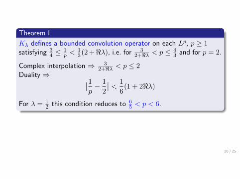
Theorem I

Kλ defines a bounded convolution operator on each Lp, p ≥ 1satisfying 3

4 ≤1p <

13(2 +<λ), i.e. for 3

2+<λ < p ≤ 43 and for p = 2.

Complex interpolation ⇒ 32+<λ < p ≤ 2

Duality ⇒ ∣∣1p− 1

2

∣∣ < 1

6(1 + 2<λ)

For λ = 12 this condition reduces to 6

5 < p < 6.

20 / 25

Theorem II

Let 65 < q < 6 and |u∞| ≤ 1

2 . Furthermore, let G ∈ Lq(R3) and letF = div Φ where Φ, (ω ∧ y) · ∇Φ, u∞ · ∇Φ ∈ Lq(R3)

⇒ the linear problem has a unique solution g ∈ Lq(R3) such that

‖g‖q ≤ c(‖G‖q + ‖ωΦ‖q + ‖(ω ∧ y) · ∇Φ‖q + ‖u∞ · ∇Φ‖q

)

Get v, σ from the system

−µ∆v + (u∞ − ω ∧ y) · ∇v + ω ∧ v +∇σ = F + (µ+ ν)∇gdiv v = g

Theorem III

Let F = div Φ, g as before, let 65 < q < 6. Then v, σ satisfy

‖∇2v‖q + ‖∇σ‖q

≤ c(‖F + (µ+ ν)∇g‖q + ‖µ∇g + (ω ∧ y)g − u∞g‖q

)

21 / 25

Theorem II

Let 65 < q < 6 and |u∞| ≤ 1

2 . Furthermore, let G ∈ Lq(R3) and letF = div Φ where Φ, (ω ∧ y) · ∇Φ, u∞ · ∇Φ ∈ Lq(R3)

⇒ the linear problem has a unique solution g ∈ Lq(R3) such that

‖g‖q ≤ c(‖G‖q + ‖ωΦ‖q + ‖(ω ∧ y) · ∇Φ‖q + ‖u∞ · ∇Φ‖q

)

Get v, σ from the system

−µ∆v + (u∞ − ω ∧ y) · ∇v + ω ∧ v +∇σ = F + (µ+ ν)∇gdiv v = g

Theorem III

Let F = div Φ, g as before, let 65 < q < 6. Then v, σ satisfy

‖∇2v‖q + ‖∇σ‖q

≤ c(‖F + (µ+ ν)∇g‖q + ‖µ∇g + (ω ∧ y)g − u∞g‖q

) 21 / 25

References

• R. Farwig, M. Pokorny: TU Darmstadt, Preprint (2014)——• S. Kracmar, S. Necasova, A. Novotny, A.: Ann. Univ. Ferrara

(2014)——• R. Danchin: Invent. Math. (2000)• F. Charve, R. Danchin: Arch. Ration. Mech. Anal. (2010)——• T. Kobayashi, Y. Shibata: Comm. Math. Phys. (1999)• Y. Shibata, K. Tanaka: J. Math. Soc. Japan (2003)• Y. Shibata, K. Tanaka: Math. Methods Appl. Sci. (2004)• Y. Enomoto, Y. Shibata: Funkcial. Ekvac. (2013)• Y. Enomoto, L. von Below, Y. Shibata, Yoshihiro. Ann. Univ.

Ferrara (2014)

22 / 25

International Research Training Group 1529

Mathematical Fluid Dynamics

Bad Boll, GermanyBad Boll, GermanyOctober 27 – 30, 2014October 27 – 30, 2014

Lecture SeriesLecture Series

Peter Constantin, PrincetonPeter Constantin, PrincetonPDE Problems of Hydrodynamic OriginPDE Problems of Hydrodynamic Origin

Yasunori Maekawa, SendaiYasunori Maekawa, SendaiAnalysis of Incompressible Flows in Unbounded DomainsAnalysis of Incompressible Flows in Unbounded Domains

László Székelyhidi, LeipzigLászló Székelyhidi, LeipzigThe h-Principle in Fluid Mechanics and Onsager's ConjectureThe h-Principle in Fluid Mechanics and Onsager's Conjecture

For further information please visit:www.mathematik.tu-darmstadt.de/~igk/badboll2014or contact: Verena Schmid, +49 6151 16 4694,[email protected]

M. Kyed (Kassel)M. Kyed (Kassel)M. Lopes Filho (Rio de Janeiro)M. Lopes Filho (Rio de Janeiro)P. Maremonti (Naples)P. Maremonti (Naples)P. Mucha (Warsaw)P. Mucha (Warsaw)Š. Nečasová (Prague)Š. Nečasová (Prague)J. Prüss (Halle)J. Prüss (Halle)M. Schoenbek (Santa Cruz)M. Schoenbek (Santa Cruz)F. Sueur (Paris)F. Sueur (Paris)R. Takada (Sendai)R. Takada (Sendai)W. Varnhorn (Kassel)W. Varnhorn (Kassel)E. Zatorska (Warsaw)E. Zatorska (Warsaw)

Autumn School and WorkshopAutumn School and Workshop

Confirmed SpeakersConfirmed Speakers

K. Abe (Nagoya)K. Abe (Nagoya)H. Abels (Regensburg)H. Abels (Regensburg)D. Bothe (Darmstadt)D. Bothe (Darmstadt)L. Brandolese (Lyon)L. Brandolese (Lyon)R. Danchin (Paris)R. Danchin (Paris)K. Disser (Berlin)K. Disser (Berlin)R. Farwig (Darmstadt)R. Farwig (Darmstadt)E. Feireisl (Prague)E. Feireisl (Prague)T. Hishida (Nagoya)T. Hishida (Nagoya)J. Kelliher (Los Angeles)J. Kelliher (Los Angeles)H. Koch (Bonn)H. Koch (Bonn)

Organizers:Organizers:

M. HieberM. HieberH. KozonoH. Kozono 23 / 25

From Incompressibility to Compressibility

Standard estimates for incompressible fluid flow around/past arotating obstacle:

1 < q <∞

Estimates for compressible fluid flow around/past a rotatingobstacle:

Only for6

5< q < 6

24 / 25

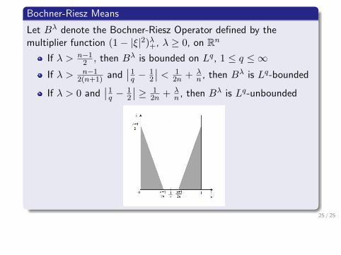
Bochner-Riesz Means

Let Bλ denote the Bochner-Riesz Operator defined by themultiplier function (1− |ξ|2)λ+, λ ≥ 0, on Rn

If λ > n−12 , then Bλ is bounded on Lq, 1 ≤ q ≤ ∞

If λ > n−12(n+1) and

∣∣1q −

12

∣∣ < 12n + λ

n , then Bλ is Lq-bounded

If λ > 0 and∣∣1q −

12

∣∣ ≥ 12n + λ

n , then Bλ is Lq-unbounded

25 / 25

The fundamental solution of compressible and ...

Documents

Transcript of The fundamental solution of compressible and ...