University of New MexicoUNM Digital Repository

Electrical and Computer Engineering ETDs Engineering ETDs

2-8-2011

The Fundamental Resonant Frequency andRadiation Characteristics of Wide Angle ConicalAntennasJulie E. Lawrance

Follow this and additional works at: https://digitalrepository.unm.edu/ece_etds

This Thesis is brought to you for free and open access by the Engineering ETDs at UNM Digital Repository. It has been accepted for inclusion inElectrical and Computer Engineering ETDs by an authorized administrator of UNM Digital Repository. For more information, please contactdisc@unm.edu.

Recommended CitationLawrance, Julie E.. "The Fundamental Resonant Frequency and Radiation Characteristics of Wide Angle Conical Antennas." (2011).https://digitalrepository.unm.edu/ece_etds/152

i

ii

iii

iv

THE FUNDAMENTAL RESONANT FREQUENCY

AND RADIATION CHARACTERISTICS OF

WIDE ANGLE CONICAL ANTENNAS

by

Julie E. Lawrance

B.S., Physics, Occidental College, 1985

M.S., Electrical Engineering, University of New Mexico, 2010

ABSTRACT

Of recent interest for simple compact pulse power systems is the self-resonant wide-angle

conical antenna. In its typical application, this antenna will radiate a transient damped

sine wave pulse whose center frequency is the fundamental resonant frequency of the

antenna. In order to properly design such an antenna, it is important to know the

dependence of the fundamental resonant frequency on both slant height and half cone

angle. Theoretical analysis of this type of antenna is typically based on the mode theory

of antennas (as derived by S.A. Schelkunoff) in which the structure is treated as a conical

transmission line. The theory is quite complicated and leads to two sets of equations

involving infinite sums which must be solved simultaneously; this is a difficult task.

In this effort, the accuracy of simplifications to the theory in predicting the fundamental

resonant frequency of a wide angle conical antenna was explored by comparing the

results obtained based on these approximations to experimental results as well as the

results of numerical simulation using CST Microwave Studio. Good agreement is

obtained between the simulated and experimentally measured results.

It was found that a first order approximation to the theory as derived by C. Papas and R.

King, while otherwise very useful, is insufficient to predict the fundamental resonant

frequency of a wide angle conical antenna with reasonable accuracy; however, a second

order approximation as derived by P.D.P. Smith does yield results that are in good

v

agreement with results of experiment and simulation. It was found that the relationship

between slant height (ℓ) and wavelength (λ) at the fundamental resonant frequency, for

wide half cone angles, corresponds more closely to ℓ= λ /8 than the expected ℓ= λ /4.

Of primary interest was the fundamental resonant frequency as a function of slant height

and half cone angle; however, the peak radiated electric field and the radiation efficiency

of the conical antenna as a function of half cone angle was also explored.

vi

Table of Contents

1. INTRODUCTION AND BACKGROUND ................................................................... 1

2. THEORETICAL ANALYSIS OF THE ELECTRICALLY SMALL WIDE ANGLE

BICONE ANTENNA ......................................................................................................... 5

2.1 An Outline of the Mode Theory of Antennas Applied to the Biconical Dipole (S.A.

Schelkunoff) .................................................................................................................... 6

2.1.1 Fundamental Resonance Obtained from First Order Approximation to the

Theory (C. Papas and R. King) ................................................................................. 10

2.1.2 Fundamental Resonance Obtained From the Second Order Approximation to

the Theory (P. D. P. Smith) ....................................................................................... 15

3. NUMERICAL SIMULATION ................................................................................. 19

3.1 Fundamental Resonance of Wide Angle Monocone Antenna Over an Infinite

Ground Plane ................................................................................................................ 20

3.2 Radiation Characteristics of Wide Angle Monocone Antenna Over an Infinite

Ground Plane ................................................................................................................ 27

3.2.1 Peak Electric Field at r=5m .............................................................................. 27

3.2.2 Radiation Efficiency vs. Half Cone Angle ....................................................... 29

3.2.3 Gain and Beamwidth at Resonant Frequency .................................................. 35

4. EXPERIMENTAL RESULTS OF G.H. BROWN & O.M. WOODWARD AND

COMPARISON WITH RESULTS OF THEORY AND SIMULATIONS ...................... 37

4.1 Fundamental Resonance of Wide Angle Conical Antennas Obtained from

Experiments of G. Brown and O. Woodward ............................................................... 37

5. EXPERIMENTS CONDUCTED BY J.E. LAWRANCE TO EXPLORE

FUNDAMENTAL RESONANT FREQUENCY ............................................................. 40

6. SUMMARY .............................................................................................................. 47

7. CONCLUSION ......................................................................................................... 49

8. REFERENCES ......................................................................................................... 50

Appendix A. Matlab Program to Evaluate Input Impedance from Theory ....................... 52

Appendix B: Effect of Finite Ground Plane (Simulation with CST Microwave Studio) . 54

Appendix C: Resonant Frequency and Radiation Characteristics of Bicone Antenna ..... 57

vii

List of Figures

Figure 1. Compact Pulse Power System with Self-Resonant Bicone Antenna ................... 3

Figure 2. Diagram of a Spherically Capped Biconical Antenna ......................................... 7

Figure 3. Spherically Capped Monocone Fed by a Matched Coaxial Line with Infinite

Ground Flange .................................................................................................................. 10

Figure 4. Input Resistance as a Function of ka for 30° Half Cone Angle ......................... 12

Figure 5. Input Reactance as a Function of ka for 30° Half Cone Angle ......................... 13

Figure 6. ka at Fundamental Resonant Frequency vs. Half Cone Angle (Predicted from

Equations of Papas and King) ........................................................................................... 14

Figure 7. Subscript n as a function of cos(α) reproduced from [7] ................................... 17

Figure 8. Input Resistance and Reactance Calculated by P.D.P. Smith ............................ 18

Figure 9. Hollow Copper Monocone Used in Numerical Simulations ............................. 19

Figure 10. Excitation Signal Used in Simulations ............................................................ 20

Figure 11. Simulated Electric field for a 15º Half Cone Angle (Time Domain) .............. 21

Figure 12. Simulated Electric Field for a 15° Half Cone Angle (Frequency Domain) ..... 22

Figure 13. ka at Fundamental Resonance vs. Half Cone Angle........................................ 23

Figure 14. Gaussian Input Signal For S11 Measurements (Time Domain) ...................... 24

Figure 15. Gaussian Input Signal for S11 Measurements (Frequency Domain) .............. 24

Figure 16. S11 Measurement 45 Deg Half Cone Angle (1 Ohm Port Impedance)........... 25

Figure 17. S11 Measurement 45 Deg Half Cone Angle (53 Ohm Port Impedance)......... 25

Figure 18. Smith Chart Representation of Simulated S11 ................................................ 26

Figure 19. Peak Far Field Electric Field for a 45° Half Cone Angle ................................ 27

Figure 20. Peak Electric Field in Far-Zone Along Radial Axis ........................................ 28

Figure 21. Divide Volume Between Cone and Groundplane into n x p Annular Ring .... 29

Figure 22. Total Capacitance of a Monocone over a Groundplane .................................. 31

Figure 23. Stored Energy as a Function of Half Cone Angle (Charge Voltage = 1 V) .... 32

Figure 24. E(t) @ r=5m, Half Cone Angle=5° ................................................................. 33

Figure 25. Radiated Pulse Total Energy Density for a Half Cone Angle of 5 Degrees .... 33

Figure 26. Radiation Efficiency (Total Pulse Energy in J/m2 per Joule of Stored Charge)

.......................................................................................................................................... 34

Figure 27. Relative Radiation Efficiency as a Function of Half Cone Angle ................... 34

Figure 28. Radiation Pattern for Hollow Cone Over Infinite Groundplane (α=45°) ........ 35

Figure 29. Polar Plot Representation of Radiation Pattern (5° Half Cone Angle) ............ 35

viii

Figure 30. Experimentally Determined Reactance as a Function of Monocone Slant

Height................................................................................................................................ 38

Figure 31. Comparison of Results (Experiment, Theory, and Simulation [CST MWS] .. 39

Figure 32. Schematic Diagram of Experimental Setup ..................................................... 40

Figure 33. High Voltage Charge Pulse ............................................................................. 41

Figure 34. Monocones and Monopole Used In Experiments (α=0°, 10.2°, 42°) ............... 42

Figure 35. Time Domain Electric Field (Monopole of Finite Thickness) ........................ 43

Figure 36. Frequency Domain Electric Field (Monopole of Finite Thickness) ................ 43

Figure 37. Time Domain Electric Field (α=10°, a=.3m5) ................................................. 44

Figure 38. Frequency Domain Electric Field (α=10°, a=.35m) ........................................ 44

Figure 39. Time Domain Electric Field (α=42°, a=.3m) ................................................... 45

Figure 40. Frequency Domain Electric Field (α=42°, a=.3m) .......................................... 45

Figure 41. Fundamental Resonance of a Conical Antenna ............................................... 48

Figure 42. Hollow Cone Over Finite Ground Plane (ground plane radius = 0.3m) .......... 54

Figure 43. Radiated Electric Field, Finite Ground Plane .................................................. 54

Figure 44. Ground Plane Radius = 0.3 meters. ................................................................. 55

Figure 45. Ground Plane Radius = 0.6 meters .................................................................. 55

Figure 46. Ground Plane Radius = 0.9 meters .................................................................. 55

Figure 47. Ground Plane Radius = 1.2m .......................................................................... 55

Figure 48. 30° Bicone Antenna (Slant Height = 0.3 m) .................................................... 57

Figure 49. Radiated Pulse for Bicone with 30° Half Cone Angle .................................... 57

Figure 50. Radiation Pattern for a 30° Bicone Antenna ................................................... 58

Figure 51. Polar Plot of Radiation Pattern ........................................................................ 58

ix

List of Tables

Table 1. Calculated Value of ka for first resonance as a function of half cone angle ....... 13

Table 2. Summary of Results from Modelling with CST Microwave Studio .................. 23

Table 3. Gain and Main Lobe Half Power Beamwidth at Resonant Frequency ............... 36

Table 4. Summary of Experimental Results ..................................................................... 46

Table 5. Effect of Finite Ground Plane on the Fundamental Resonant Frequency ........... 56

1

1. INTRODUCTION AND BACKGROUND

The wide-angle conical antenna is among the more interesting and useful

canonical problems in antenna theory. Analysis of this type of antenna is typically

based on the mode theory of antennas in which the structure is treated as a conical

transmission line. It is relatively straightforward for large half-cone angles if the

slant height of the cone is very large compared to a wavelength [1, 2]; in this case

the antenna can be viewed as a uniform conical transmission line.

Of recent interest for compact pulse power systems is the self-resonant wide-

angle conical antenna. In this application, the slant height is a fraction of a

wavelength at the fundamental resonant frequency. The distributed impedance of

the conical transmission line is no longer uniform but rather it is significantly

modified by radiation.

The mode theory of antennas as applied to this structure was derived by S.A.

Schelkunoff [3, 4] and is outlined in Section 2.1. It reduces the problem to one of

deriving a terminating admittance at the ends of the cone by subjecting

characteristic solutions to Maxwell’s equations - which are valid for the reflected

and radiated waves at the ends of the cone - to the appropriate boundary

conditions. This approach ultimately leads to two sets of equations involving

summations of infinite series which are the eigenfunction expansions of the non-

vanishing radiated and reflected electric- and magnetic- field vectors. These must

be simultaneously solved to determine the coefficients of expansion. This is

virtually an impossible task.

A significant simplification to the theoretical model is obtained by assuming that

a single TEM mode exists inside of the conical transmission line [5, 6]; radiated

fields are then expanded in a series of eigenfunctions. This will be referred to in

this paper as the “first order approximation” and is presented in Section 2.1.1.

2

Including just a single “complementary wave”1 within the region of the conical

transmission line in addition to the TEM mode as well as two outward

propagating complementary waves greatly increases the complexity of the

governing equations; however it has been accomplished and the results are

available in the literature [7, 8]. This will be referred to as the “second order

approximation” and is presented in Section 2.1.2.

The validity of the first and second order approximations to the theoretical model

was explored by comparing the results obtained based on these simplifications to

those of experimental measurement (presented in Section 4) and numerical

modeling(presented in Section 3)2.

Of primary interest were the fundamental resonant frequency and the peak

radiated electric field as measured along the radial axis in the far-field as a

function of half cone angle ranging from 5-85°. Good agreement is obtained

between the simulated and measured results. It was found that the first order

approximation to the theory is insufficient to predict the fundamental resonant

frequency of a wide angle conical antenna with reasonable accuracy; however the

second order approximation does yield results that are in quite good agreement

with results of experiment and numerical modeling.

Wide-angle, self-resonant conical antennas are particularly well-suited to simple

compact pulse power systems. In this type of system, the antenna is charged to

high voltage by a voltage source such as a Marx generator, and a self break switch

is incorporated at the apex of the cone to initiate oscillation of the stored charge.

The radiated waveform from these systems is a transient; specifically, a damped

sine wave with a center frequency determined by the dimensions of the cone.

1 As defined by S. A. Schelkunoff [9], “principal waves” are waves which would exist in an

infinitely long antenna and “complementary waves” are waves which are generated at a

discontinuity, such as an electrically small bicone antenna. 2 Some experimental results were obtained from the literature [10]; however, further laboratory

experiments and all simulations were conducted by J. Lawrance as part of this effort.

3

There are several important considerations that go into the design of such

antennas:

1. It must be able to store energy from a voltage source (i.e., it must have

a relatively large capacitance),

2. It must radiate the stored energy once the switch is closed, and

3. It must be designed to resonate at the desired center frequency.

The desired radiated waveform from these systems is a damped sine wave with a

Q of about 5-6 and a relatively low center frequency – on the order of 100-500

MHz. In this application, the slant height of the cone is a fraction of a wavelength

at some desired center frequency. An example of a compact wideband radiator

employing a self-resonant bicone antenna [11] is shown in the photograph of

Figure 1.

Figure 1. Compact Pulse Power System with Self-Resonant Bicone Antenna

The antenna is charged to high voltage by a 300kV Marx generator. Power

supplies are built into the interior volume of the cones. A self-break switch in oil

located between the two cones is employed to initiate oscillation of the stored

4

charge and subsequent radiation from the source. The result is a very compact,

portable, wideband pulse radiator that weighs less than 20 lbs.

As mentioned previously, the antenna plays a unique role in such a system; i.e., in

addition to being the radiating element, it is also the energy storage device and its

dimensions determine the center frequency of the radiated waveform. In

designing a conical antenna for a simple compact pulse power source such as

described here, it is desirable to determine the appropriate slant height and half

cone angle which will produce the desired center frequency of the radiated wave

with maximum radiation efficiency.

5

2. THEORETICAL ANALYSIS OF THE ELECTRICALLY SMALL

WIDE ANGLE BICONE ANTENNA

The problem of the wide angle conical antenna lends itself most readily to the

“mode theory” of antennas as presented by S. A. Schelkunoff [3]. This theory is

outlined in Section 2.1 to illustrate the complexity of the governing equations

derived using this approach. These equations are very difficult to solve

analytically; however for a few specific antenna geometries, certain assumptions

can be made which make these equations more manageable3.

In the case of the electrically small wide-angle bicone antenna (or monocone

antenna over a ground plane), where the half cone angle is 5-85°, such

assumptions are no longer applicable and the task becomes more difficult.

In order to determine the input impedance wide-angle conical dipole of finite

length, C. Papas and R. King [5] derived a simplified set of equations by

assuming that only the fundamental TEM mode exists in the region of the conical

transmission line and that higher order modes are negligible. Their results are

summarized in Section 2.1.1. This first order approximation yields sufficiently

accurate results for some purposes [16-18]. However, when compared to the

results of simulation and experiment (presented in Sections 3 and 4, respectively),

it was found that it does not accurately predict the fundamental resonance of a

wide angle conical antenna, which is of primary interest for this effort.

P.D.P Smith tackled the problem of including just one additional complementary

wave (in addition to the TEM wave) and two complementary outward

propagating waves in his analysis [7]. His derivation and results are presented in

3 This theoretical approach has been successfully applied in the analysis of the electromagnetic

behavior of electrically small bicone antennas where the half cone angle is on the order of 5° or

less [Ref. 12, 13] as well as to explore the forced oscillations of the cylindrical conductor and the

prolate spheroid [Ref 14,15].

6

Section 2.1.2. These results more accurately predict the fundamental resonant

frequency of a wide angle conical antenna when compared with results of

simulation and experiment. Again, however, in this second order approximation,

with just the inclusion of these two additional waves, the equations become

significantly more complicated4.

2.1 An Outline of the Mode Theory of Antennas Applied to the Biconical

Dipole (S.A. Schelkunoff)

The mode theory of antennas is based on describing modes of propagation by

simple conventional transmission line diagrams, as derived by S.A. Schelkunoff

[3] and summarized here. The analysis is similar to that used for waveguides. In

this approach, a terminal admittance, yt, is defined as:

’

where is the slant height of the cone and,

V0(r)=V0( )cosβ( -r) + jKI0( )sinβ( -r),

I0(r)=I0( )cosβ( -r) + jK-1

V0( )sinβ( -r),

Here, K is the characteristic impedance of the conical transmission line

determined from:

for a bicone antenna, where α ≡ half cone angle (see Fig. 2).

The input impedance is then determined by transforming to the apex of the cone

via:

It should be noted here that, to determine the fundamental resonance of a conical

antenna used in the application of interest in this effort, one needs only to

4 C.T. Tai, in his paper entitled “On the Theory of Biconical Antennas” [19] presents a comparison

of calculated input impedance of a bicone antenna by inclusion of up to three higher modes in the

analysis.

(1)

(2)

(3)

(4)

(5)

7

determine the minimum value for β for which the imaginary component of the

input impedance (i.e., the input reactance) is zero. The complexity of the

equations however, makes determining the input admittance quite difficult. This is

illustrated in this section which outlines Schelkunoff’s derivation of the equations

for the non-vanishing electric-and magnetic field vectors.

The electric- and magnetic- field intensities are related to V0 and I0 by

where,

and V(r) is obtained by integrating Eθ along a meridian as shown in Figure 2. Also

indicated in Figure 2 is a “boundary sphere” which encloses the conical antenna

(just) and at which various boundary conditions may be applied.

Figure 2. Diagram of a Spherically Capped Biconical Antenna

(with Half Cone Angle = α and Slant Height = )

boundary sphere

α

spherical cap

input

meridian

(5)

(6)

(7)

8

Two regions are defined: one inside of the boundary sphere and one outside. The

following boundary conditions are applied (as reproduced from [3]):

1. In the antenna region, the tangential E must vanish at the surface of the

antenna.

2. The field in the antenna region must join continuously the field in the

free space region.

3. The field tangential to the ends of the antenna must vanish .

For condition 3 above, Shelkunoff assumes a spherical cap over the ends of the

dipole as indicated in Figure 2. If only radial currents are taken into account, the

only non-vanishing fields are Eθ, Er, and Hφ.

Fitting characteristics solutions to Maxwell’s equations to the two regions inside

and outside of the boundary sphere results in three equations in each region,

specifically;

Inside the sphere:

where

V(r)=V( )[cosβ( -r) + jKytsinβ( -r)],

KI0(r)=I0( )cosβ( -r) + jK-1V0( )sinβ( -r),

,

α=half cone angle,

,

(8)

(9)

(10)

(11)

(12)

(13)

(14)

(15)

9

Mn(cosθ) is an odd Legendre function defined by:

And the summation is carried out over all the zeros of Mn(cosθ).

The normalized Bessel functions of order n are defined by Schelkunoff in terms

of ordinary Bessel functions as:

Outside of the sphere:

Rk(βr)=Hnk(βr)

The problem becomes one of simultaneously solving these equations for an and bk

which is quite a daunting task.

(16)

(17)

(18)

(19)

(20)

(21)

(22)

10

2.1.1 Fundamental Resonance Obtained from First Order

Approximation to the Theory (C. Papas and R. King)

Based on the work of S.A. Schelkunoff [3-4] and C.T. Tai [13], C. Papas and R.

King [5] evaluated the input impedance of a spherically-capped, monocone

antenna5, fed by a coaxial conductor with an infinite ground flange, matched to

the input impedance of the cone, as shown in Figure 3.

Figure 3. Spherically Capped Monocone Fed by a Matched Coaxial Line with Infinite

Ground Flange

Papas and King used a transmission line analogy and considered only a single

TEM mode in the region of the conical transmission line. In this approach, the

5 The resonant frequency of a monocone over a ground plane is the same as that of a bicone with

the same half cone angle and slant height (refer to Appendix C).

11

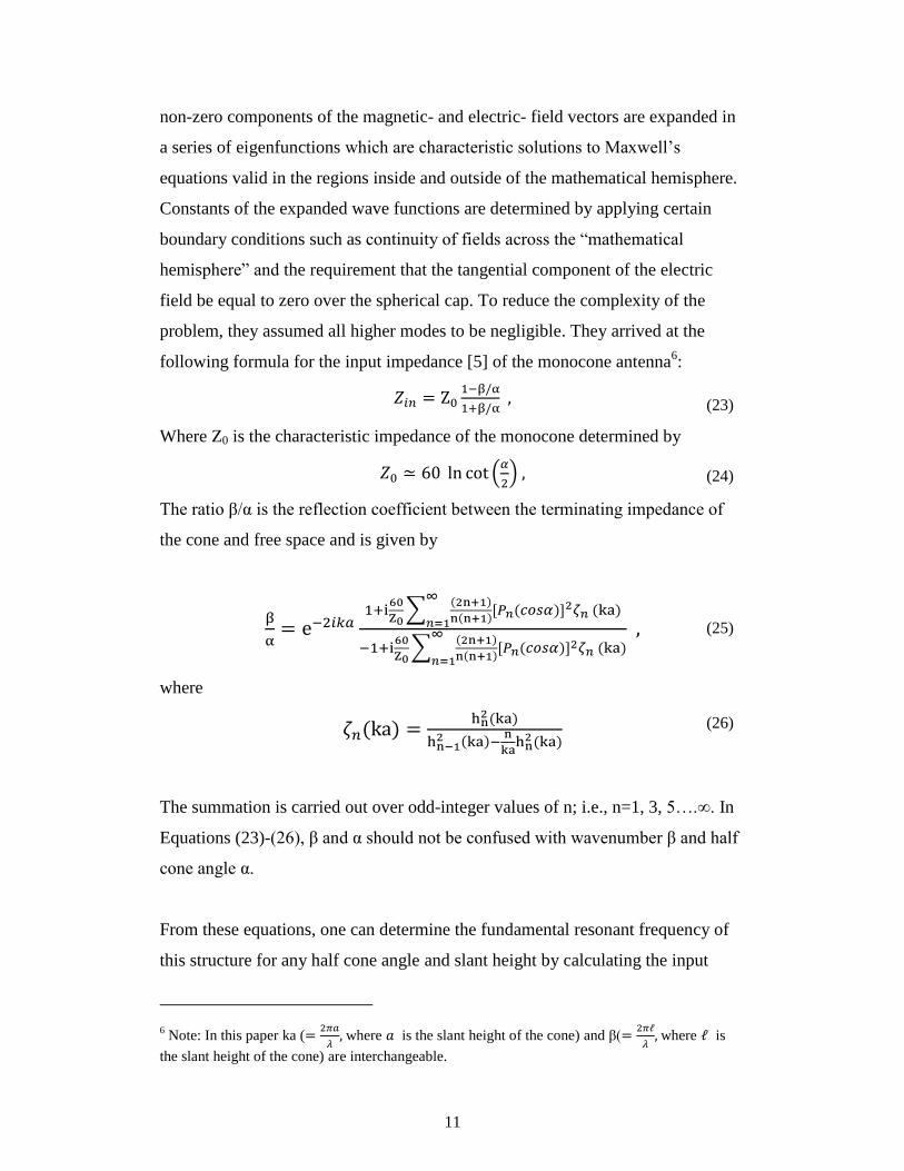
non-zero components of the magnetic- and electric- field vectors are expanded in

a series of eigenfunctions which are characteristic solutions to Maxwell’s

equations valid in the regions inside and outside of the mathematical hemisphere.

Constants of the expanded wave functions are determined by applying certain

boundary conditions such as continuity of fields across the “mathematical

hemisphere” and the requirement that the tangential component of the electric

field be equal to zero over the spherical cap. To reduce the complexity of the

problem, they assumed all higher modes to be negligible. They arrived at the

following formula for the input impedance [5] of the monocone antenna6:

Where Z0 is the characteristic impedance of the monocone determined by

The ratio β/α is the reflection coefficient between the terminating impedance of

the cone and free space and is given by

where

The summation is carried out over odd-integer values of n; i.e., n=1, 3, 5….∞. In

Equations (23)-(26), β and α should not be confused with wavenumber β and half

cone angle α.

From these equations, one can determine the fundamental resonant frequency of

this structure for any half cone angle and slant height by calculating the input

6 Note: In this paper ka (

where is the slant height of the cone) and β(

where is

the slant height of the cone) are interchangeable.

(23)

(24)

(25)

(26)

12

impedance over a range of values of ka and determining the minimum value of ka

for which the reactance (i.e., the imaginary component of this impedance) is zero.

A simple Matlab program was written (refer to Appendix A) to evaluate input

resistance and reactance based on the equations of Papas and King for a range of

half-cone angles as a function of ka, where k=2π/λ and a is the slant height of the

cone. The summations were carried out to n=21, which is more than sufficient to

ensure convergence. An example of results is shown in Figure 4 and Figure 5

which present resistance and reactance calculated from the theory as a function of

ka for a half cone angle of 30 degrees.

Figure 4. Input Resistance as a Function of ka for 30° Half Cone Angle

In Figure 4, it can be seen that the resistance oscillates about the characteristic

impedance as ka increases and for large ka, it approaches the characteristic

impedance of the cone as one might expect. In Figure 5, it can be seen that the

reactance oscillates about zero as ka increases and tends to zero for large ka.

Fundamental resonance occurs at the minimum value of ka for which the

reactance is zero.

13

Figure 5. Input Reactance as a Function of ka for 30° Half Cone Angle

The values for ka which correspond to the fundamental resonant frequency

determined from the equations derived by Papas and King are presented in Table

1 below.

α(degrees) ka

5 1.25

10 1.22

20 1.21

30 1.21

45 1.21

60 1.21

70 1.22

75 1.24

80 1.28

85 1.37

90 1.57

Table 1. Calculated Value of ka for first resonance as a function of half cone angle

14

The calculated values of ka for fundamental resonance are also presented as a

function of half cone angle in Figure 6, along with ka for a =λ/4 and a=λ/5 (shown

by dashed lines). For a uniform transmission line, first resonance is expected at a=

λ/4 (ka=1.57). It is evident in this graph that first resonance predicted from the

first order approximation of Papas and King occurs at closer to a=λ/5 (ka=1.26)

over half cone angles from 5-80º. In the limit, as the half cone angle approaches

90 degrees, ka approaches 1.57, corresponding to resonance at a= λ/4, as one

would expect for a radial transmission line.

Figure 6. ka at Fundamental Resonant Frequency vs. Half Cone Angle (Predicted from

Equations of Papas and King)

It can be seen that the simplified theory predicts a starting point for slant height in

the design of a self resonant antenna at around a=λ/5 for half cone angles between

10 and 80°. This is significantly less than the quarter wave resonance one would

expect for a uniform transmission line.

0.5

0.7

0.9

1.1

1.3

1.5

1.7

0 20 40 60 80 100

ka

Half Cone Angle (Degrees)

ka at First Resonance vs. Half Cone Angle

ka (calculated)

ka (a=lambda/4)

ka (a=lambda/5)

15

2.1.2 Fundamental Resonance Obtained From the Second Order

Approximation to the Theory (P. D. P. Smith)

P.D.P Smith, in a paper published in 1947 [7], uses the same transmission line

analogy of Papas and King, but takes the theory a step further by including just

one higher order term in addition to the TEM mode (for both of the regions inside

and outside of the “mathematical sphere” indicated in Figure 1). In doing so, the

complexity of the problem is greatly increased.

Smith evaluates the terminating admittance, yt, at a distance of λ/4 from the end of

a conical transmission line and then ultimately transforms this to the apex of the

cone to arrive at the input impedance.

Just to illustrate the increased degree of complexity introduced by considering just

a single higher order term in each of the two regions, he arrived at the following

equation for K2yt (which corresponds to the cone impedance 1/4λ from the ends

of the cone):

where K is the characteristic impedance, as defined by Equation 13 and:

,

,

,

(27)

(28)

(29)

(30)

(31)

(32)

(33)

16

The subscript “n” corresponds to expansion of r∙Eθ inside the “mathematical

hemisphere” in terms of reflected waves near the ends; namely:

And the subscript “k” refers to expansion of r∙Eθ in terms of outwardly

propagating waves in the region just outside of the “mathematical hemisphere”:

The high degree of complexity of this problem is manifested when one attempts

to simultaneously solve these equations at r=l for the constants an and bk by

applying the boundary conditions of continuity of fields at the mathematical

boundary and the vanishing of the electric field over the spherical cap.

The subscript “n” is not an integer but rather it is a function of cos(α) and

corresponds to the roots of Ln(cos(α))=0 where Ln satisfies Legendre’s equation.

The value for the first root n as a function of μ=cos(α) is reproduced in Figure 7

below in the curve labeled “n1(μ1)”.

(34)

(35)

(36)

17

Figure 7. Subscript n as a function of cos(α) reproduced from [7]

The results obtained by P.D.P. Smith for the input impedance of a wide angle

cone are reproduced in Figure 8 below. In these calculations, only the first root of

Ln(cos(α))=0 and only k=1,3 were taken into account. These were obtained by

first calculating K2yt from the equation above, corresponding to the impedance at

a distance of 1/4λ from the ends of the cone, and transforming this to the apex of

the cone.

18

Figure 8. Input Resistance and Reactance Calculated by P.D.P. Smith

(reproduced from [7].)

The reactance curves in the right hand side graph of Figure 8 indicate that the

fundamental resonance (corresponding to the first zero crossing for the larger half

cone angles of 20.2°, 38.2° and 50.6°) occur at a value of ka of between 0.8 and

0.9. This is significantly different from the results obtained using the first order

approximation of Papas and King (refer to Figure 6).

19

3. NUMERICAL SIMULATION

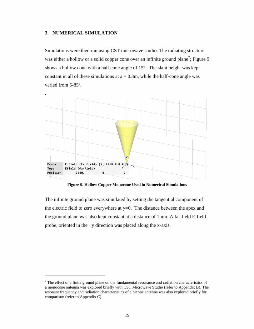
Simulations were then run using CST microwave studio. The radiating structure

was either a hollow or a solid copper cone over an infinite ground plane7; Figure 9

shows a hollow cone with a half cone angle of 15º. The slant height was kept

constant in all of these simulations at a = 0.3m, while the half-cone angle was

varied from 5-85º.

.

Figure 9. Hollow Copper Monocone Used in Numerical Simulations

The infinite ground plane was simulated by setting the tangential component of

the electric field to zero everywhere at y=0. The distance between the apex and

the ground plane was also kept constant at a distance of 1mm. A far-field E-field

probe, oriented in the +y direction was placed along the x-axis.

7 The effect of a finite ground plane on the fundamental resonance and radiation characteristics of

a monocone antenna was explored briefly with CST Microwave Studio (refer to Appendix B). The

resonant frequency and radiation characteristics of a bicone antenna was also explored briefly for

comparison (refer to Appendix C).

20

3.1 Fundamental Resonance of Wide Angle Monocone Antenna Over an

Infinite Ground Plane

The excitation signal is shown in Figure 10. This voltage signal had a slow rise

time of 10ns corresponding to the charging phase, a hold time of 5ns to ensure the

cone was fully charged and a fast fall time of 100 ps, corresponding to closing of

the self break switch which would be employed in a real system. The voltage was

then held to zero for another 55ns or more to ensure this point was “shorted” for

the duration of the measured excitation. Again, this corresponds to realistic

conditions in an actual system.

Figure 10. Excitation Signal Used in Simulations

The measured far-field, vertically polarized electric field radiated from the conical

antenna with this excitation signal for a 15º half cone angle is shown in Figure 11.

21

Figure 11. Simulated Electric field for a 15º Half Cone Angle (Time Domain)

The resulting radiated waveform, as seen in this figure, show an initial sharp

transient spike, which is generated when the switch closes, followed by a damped

sine wave with a Q of about 5.

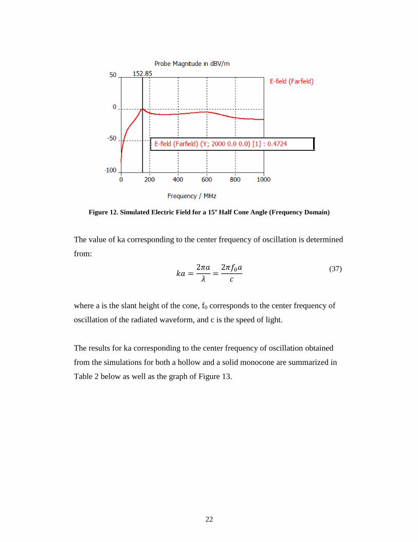
The center frequency of oscillation in this case is 153 MHz, as can be seen in the

frequency domain signal of Figure 12. Since the slant height, a, in this simulation

is 0.3m, this leads to a value for ka (=2πa/λ) of around 0.94. For comparison, the

center frequency one would expect for quarter wave resonance where a = λ/4

would be close to 250 MHz and the value for ka would be equal to 1.57.

22

Figure 12. Simulated Electric Field for a 15° Half Cone Angle (Frequency Domain)

The value of ka corresponding to the center frequency of oscillation is determined

from:

where a is the slant height of the cone, f0 corresponds to the center frequency of

oscillation of the radiated waveform, and c is the speed of light.

The results for ka corresponding to the center frequency of oscillation obtained

from the simulations for both a hollow and a solid monocone are summarized in

Table 2 below as well as the graph of Figure 13.

(37)

23

α (°) ka

(hollow cone)

ka

(solid cone)

5 1.1 1.09

15 0.96 .94

30 0.88 .85

45 0.84 .85

60 0.95 .92

70 1.04 1.01

80 1.16 1.16

85 1.22 1.22

Table 2. Summary of Results of Numerical Simulations

Figure 13. ka at Fundamental Resonance vs. Half Cone Angle

From Numerical Simulations

These results indicate a value for ka at the fundamental resonance at close to a=

λ/8 for half cone angles in the range of 30°- 50°. This is significantly different

from the values predicted by the approximation of Papas and King. Note also that

0

0.2

0.4

0.6

0.8

1

1.2

1.4

1.6

1.8

0 10 20 30 40 50 60 70 80 90

ka

Half Cone Angle (Degrees)

ka vs. Half Cone Angle at Fundamental Resonance

ka (hollow cone)

ka (solid cone)

ka(a=lambda/4)

ka(a=lambda/5)

ka(a=lambda/8)

24

there is not a significant difference in the resonant frequency between that of the

hollow and the solid cones.

S11 simulations were also made as follows: a hollow copper cone over an infinite

ground plane was excited with a broadband Gaussian signal (1MHz – 1GHz) via a

port located between the apex of the cone and ground. The Gaussian signal is

shown in the time- and frequency- domains, respectively in Figures 14 and 15.

Figure 14. Gaussian Input Signal For S11 Measurements (Time Domain)

Figure 15. Gaussian Input Signal for S11 Measurements (Frequency Domain)

25

Two S11 measurements were made for each half cone angle; first with a port

impedance of 1 ohm and then with the port impedance matched to the

characteristic impedance of the cone. Examples of measurements for a half cone

angle of 45 degrees are shown in Figures 16-18 below. In Figure 16, the resonant

frequency observed in the radiated field for this structure in the free-field

simulations (see table 2) can be seen in the S11 measurement at close to 136MHz.

Figure 16. S11 Measurement 45 Deg Half Cone Angle (1 Ohm Port Impedance)

Figure 17 presents the simulated S-Parameter measurement made with the port

impedance matched to the characteristic impedance of the cone, i.e., 53 Ω.

Figure 17. S11 Measurement 45 Deg Half Cone Angle (53 Ohm Port Impedance)

26

A dominant resonant frequency is not evident in this case because the input

impedance is matched to the cone. However, in the Smith Chart representation of

this simulated measurement, shown in Figure 18 below, one can see that the

imaginary component of the impedance first goes to zero at close to 134 MHz.

This corresponds to the resonant frequency of this structure observed in the

radiated electric field simulation (see Table 2).

Figure 18. Smith Chart Representation of Simulated S11

for Hollow Cone with Port Impedance of 53 Ω

The S11 simulations were made to establish that the fundamental resonant

frequency of a monocone over a ground plane can be obtained from the S11

measurement regardless of whether the apex of the cone is shorted or matched to

the impedance voltage source. When the impedance of the voltage source is

matched to the apex of the cone, it will not resonate of course; however, the

frequencies corresponding to zero reactance observed in the Smith Chart

representation of the measurement will reveal the fundamental (as well as higher)

resonances.

27

3.2 Radiation Characteristics of Wide Angle Monocone Antenna Over an

Infinite Ground Plane

The radiated waveform from a monocone over an infinite ground plane (as

described in section 3.1) driven at the apex by the step pulse shown in Figure 10

was simulated by placing a far field electric field probe oriented along the y axis

(i.e., vertically polarized) in the far zone at 5 meters. In addition to the E-field

probe, the full three dimensional radiation pattern was explored with an RCS far

field monitor.

3.2.1 Peak Electric Field at r=5m

The time-domain, vertical electric field at a distance of 5 meters along the radial

axis obtained from numerical simulation for a half cone angle of 45 degrees with

a step pulse excitation is presented in Figure 19. As for all of the simulated

radiated waveforms (refer to Figure 11), a very fast transient spike is evident early

on, followed by a damped sine wave at the resonant frequency over several cycles

of oscillation.

Figure 19. Peak Far Field Electric Field for a 45° Half Cone Angle

28

The peak of the damped sine wave was determined for half cone angles ranging

from 5-88°. The results are summarized in the graph of Figure 20. The peak

electric field at the resonant frequency increases relatively rapidly for half cone

angles of 5° to 30°, then increases more gradually as the half cone angle is

increased from 30° to 60°. It then increases rapidly again from 60° to 80°, after

which it appears to level off for half cone angles of 80° to 88°.

Figure 20. Peak Electric Field in Far-Zone Along Radial Axis

Associated with Damped Sine Wave

If it is desirable to achieve maximum electric field at a specific range when the

charge voltage is fixed (which it often is) the graph of Figure 20 indicates that the

broader the half-cone angle the better.

However, this is not an indication of the radiation efficiency of the conical

antenna, since for a fixed charge voltage, the antenna capacitance and therefore

the stored energy, increases with increasing half cone angle. For a true measure of

relative radiation efficiency (at a fixed point along the equator) as a function of

0

0.02

0.04

0.06

0.08

0.1

0.12

0.14

0.16

0.18

0.2

0 10 20 30 40 50 60 70 80 90

Pea

k E

lect

ric

Fie

ld

Half Cone Angle (Degrees)

E-Peak (V/m)

29

half cone angle, one must calculate the energy density of the radiated waveform

and divide this by the energy stored in the antenna.

3.2.2 Radiation Efficiency vs. Half Cone Angle

The energy (U0) stored in the cone is given by:

Where V is the charge voltage and C is the capacitance of the cone.

An estimate of the cone capacitance can be obtained from , where t is

the transit time determined from (with c = the speed of light and = the

slant height of the cone).

Perhaps a more accurate evaluation of the capacitance of a monocone over a

ground plane can be determined by dividing the volume between the cone and the

ground plane into n x p annular-ring, parallel plate capacitors along equipotential

lines and exploring the limit as n and p approach infinity. This is illustrated in the

drawing of Figure 21.

Figure 21. Divide Volume Between Cone and Groundplane into n x p Annular Ring

Parallel Plate Capacitors Along Equipotential Lines

α

l

i=1 i=n

j=1

j=p

j=2

i=2

Field Lines

Equipotential Lines

(37)

30

This results in a grid of capacitors that fill the volume of interest between the cone

and ground plane and whose plates lie along equipotential surfaces. Some of the

capacitors add in parallel and the rest add in series. If the angle between the

monocone and the ground plane (β=90-α) is divided into p equal subangles, the

capacitance of a single element is given by:

β β

If the slant height is divided into n equal increments then Δr=l/n and the

capacitance of a single element is given by

β

For each value of j, the incremental annular ring capacitors add in parallel so that

β β

As p→∞, β/p→0 and sin(β/p) → β/p, so that this equation reduced to:

The problem is reduced to finding the capacitance of the p disc capacitors as

shown in the drawing, all of which add in series. As p→∞, β/p→0 and sin(β/p) →

β/p, so that the inverse of the total capacitance is given by

Therefore,

(38)

)

(37)

(39)

(40)

(41)

(42)

(43)

31

In the limit, as n,p→∞, this becomes an exact expression for the capacitance of

this structure, ignoring fringe effects .

The results were compared to that obtained by estimating cone capacitance by

C=t/Z0 as shown in Figure 22.

Figure 22. Total Capacitance of a Monocone over a Groundplane

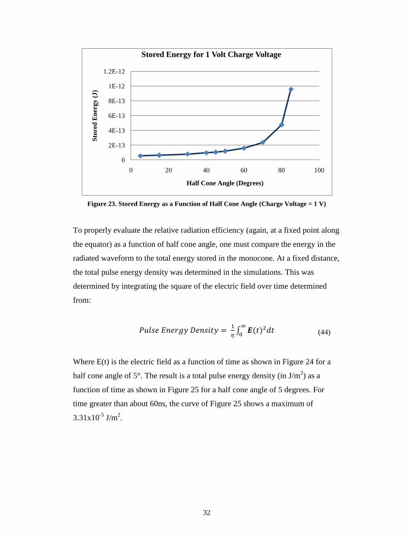
For a fixed charge voltage of 1V, as was used in the simulations, this translates to

a stored energy as a function of half cone angle as shown in Figure 23.

0.00E+00

5.00E-11

1.00E-10

1.50E-10

2.00E-10

2.50E-10

3.00E-10

0 20 40 60 80 100

Cap

acit

ance

(F)

Half Cone Angle (degrees)

Estimated Capacitance vs. Half Cone Angle

Capacitance (Based on Infinitessimal Annular Ring Parallel Plate Capacitors) *

Capacitance[C=t/Z; Z=60*ln(cot(a)/2)]

32

Figure 23. Stored Energy as a Function of Half Cone Angle (Charge Voltage = 1 V)

To properly evaluate the relative radiation efficiency (again, at a fixed point along

the equator) as a function of half cone angle, one must compare the energy in the

radiated waveform to the total energy stored in the monocone. At a fixed distance,

the total pulse energy density was determined in the simulations. This was

determined by integrating the square of the electric field over time determined

from:

Where E(t) is the electric field as a function of time as shown in Figure 24 for a

half cone angle of 5°. The result is a total pulse energy density (in J/m2) as a

function of time as shown in Figure 25 for a half cone angle of 5 degrees. For

time greater than about 60ns, the curve of Figure 25 shows a maximum of

3.31x10-5

J/m2.

0

2E-13

4E-13

6E-13

8E-13

1E-12

1.2E-12

0 20 40 60 80 100

Sto

red

En

erg

y (

J)

Half Cone Angle (Degrees)

Stored Energy for 1 Volt Charge Voltage

(44)

33

Figure 24. E(t) @ r=5m, Half Cone Angle=5°

Figure 25. Radiated Pulse Total Energy Density for a Half Cone Angle of 5 Degrees

To determine relative radiation efficiency, the calculated pulse energy density

should then be divided by the energy initially stored in antenna for the (in this

case) one volt charge voltage. The data are presented as radiated pulse energy (in

Joules/m2 per Joule of stored energy in Figure 26.

-0.08

-0.06

-0.04

-0.02

0

0.02

0.04

0.06

0.08

0 20 40 60 80 100 120 140

Ele

ctri

c F

ield

(V

/m)

time (ns)

Vertically Polarized Electric Field Measured at r=5m

Half Cone Angle = 5 °

0.00E+00

5.00E-06

1.00E-05

1.50E-05

2.00E-05

2.50E-05

3.00E-05

3.50E-05

0 20 40 60 80 100 120 140

Pu

lse

En

erg

y D

ensi

ty (

J/m

^2

)

time (ns)

Radiated Pulse Energy Density α= 5 °, r=5m

Total Energy Density = 3.31 x 10-5

J/m2

34

Figure 26. Radiation Efficiency (Total Pulse Energy in J/m2 per Joule of Stored Charge)

The normalized results are shown in figure 27. The curves of Figures 26 and 27

indicate peak radiation efficiency at a half cone angle of 45°, as one might expect.

Figure 27. Relative Radiation Efficiency as a Function of Half Cone Angle

0.00E+00

2.00E+08

4.00E+08

6.00E+08

8.00E+08

1.00E+09

1.20E+09

1.40E+09

0 10 20 30 40 50 60 70 80 90

Rad

iati

on

Eff

icie

ncy

(J

/m^

2/J

)

Half Cone Angle (Degrees)

Radiation Efficiency

(Radiated Pulse Energy Density Per Joule of Stored Energy)

0

0.2

0.4

0.6

0.8

1

1.2

0 10 20 30 40 50 60 70 80 90

Rad

iati

on

Eff

icie

ncy

(u

nit

less

)

Half Cone Angle (Degrees)

Radiation Efficiency (Normalized to Peak)

35

3.2.3 Gain and Beamwidth at Resonant Frequency

The bicone antenna is not a highly directive (and therefore not a high gain)

antenna. It usefulness is primarily as a broadband radiator. However, simulations

were run to explore the gain and radiation pattern of a monocone over an infinite

groundplane at its fundamental resonant frequency.

A representative three-dimensional radiation pattern is shown in Figure 28, for a

half cone angle of 45°. The radiation pattern was similar over the 5° to 85° range

of half cone angle. The results for all half cone angles are summarized in Table 3.

Figure 28. Radiation Pattern for Hollow Cone Over Infinite Groundplane (α=45°)

The three dimensional plot shown in Figure 28 is presented as a two dimensional

polar plot in Figure 29.

Figure 29. Polar Plot Representation of Radiation Pattern (5° Half Cone Angle)

36

It was found that the half power beamwidth of the main lobe increased slowly

from approximately 40° to 50° as the half cone angle was increased from 5° to

88° and that the gain (dBi) slowly decreased over this range from 4.9 to 4.5 dBi.

Half Cone Angle(°) G (dBi) Main Lobe Beamwidth (°)

5 4.9 41.1

15 4.8 42.3

30 4.7 43.9

45 4.8 45.4

60 4.6 47.8

70 4.5 49.7

80 4.4 51.4

85 4.4 51.9

88 4.5 50.9

Table 3. Gain and Main Lobe Half Power Beamwidth at Resonant Frequency

for Hollow Cone Over Infinite Groundplane

37

4. EXPERIMENTAL RESULTS OF G.H. BROWN & O.M. WOODWARD

AND COMPARISON WITH RESULTS OF THEORY AND

SIMULATIONS

Results of experiments conducted in the 1930’s by G.H. Brown and O. M.

Woodward were then analyzed and compared to results of numerical simulation

and the approximation of Papas and King as well as that of P.D.P. Smith.

4.1 Fundamental Resonance of Wide Angle Conical Antennas Obtained

from Experiments of G. Brown and O. Woodward

Relevant experiments were conducted by G.H. Brown and O. M. Woodward in

the 1930’s in which they measured the input impedance of a cone over a large

ground plane [10]. The measured reactance as a function of the electrical height of

the cone is reproduced in Figure 30. It is important to note that the “flare angle” α

as shown corresponds to twice the half cone angle and the antenna length as

shown is the slant height times the cosine of one half the “flare angle” α. They did

not observe a significant difference between the case of the hollow cone or the

spherically capped cone.

38

Figure 30. Experimentally Determined Reactance as a Function of Monocone Slant Height

(Reproduced from [10])

The results of these experiments (evaluated at fundamental resonance) are

compared to the results of theory and simulation in the graph of Figure 31.

39

Figure 31. Comparison of Results (Experiment, Theory, and Simulation [CST MWS]

Clearly the experimental results of Brown and Woodward agree well with the

simulation results. It is evident that the simplified equations derived by Papas and

King are insufficient to accurately predict fundamental resonance of a wide-angle

conical antenna. Agreement between the theory of Papas and King, the

experimental results of Brown and Woodward and the results of simulation is

only approached in the limits where the half cone angle is very small or very close

to 90°. The results of PDP Smith, however, do agree well with the results of

experiment and simulation.

0

0.2

0.4

0.6

0.8

1

1.2

1.4

1.6

0 10 20 30 40 50 60 70 80 90

ka

Half Cone Angle (Degrees)

Comparison of Results: Experiment, Theory, and Simulation

Simulation (CST MWS)

Experiment [Brown & Woodward]

Theory [Papas & King]

Theory [ P.D. P. Smith]

40

5. EXPERIMENTS CONDUCTED BY J.E. LAWRANCE TO EXPLORE

FUNDAMENTAL RESONANT FREQUENCY

The setup used to create the radiated damped sine wave pulse from a monocone or

a monopole antenna is shown schematically in Figure 32. The antenna was

connected to the ground plane via a self-break gas switch located at the apex. This

component was borrowed from ASR (part number ASR-TYO-001). The antenna

was charged to 10-15kV slowly over approximately 20 microseconds until the

self-break switch closed. The high voltage source was also borrowed from ASR

Corporation (part number PCG-35). The charge pulse was measured with a

Tektronix P6015 high voltage probe connected to a Tektronix TDS2024B

oscilloscope and is presented in Figure 33.

An EG&G ACD-70 free-field D-dot probe (Aeq=0.001 m2) was used to measure

the radiated pulse in the far-field. This sensor was connected through a balun

(EG&G DMB-4) as well as a 500MHz low pass filter (Minicircuits LP500) to the

input of a Tektronix DPO 7254 oscilloscope using a sampling rate of 40Gs/s.

Figure 32. Schematic Diagram of Experimental Setup

0-30kV Variable Voltage

source

41

Figure 33. High Voltage Charge Pulse

Two cones were constructed with half cone angles of 10° and 42°. In addition, the

fundamental resonant frequency of a rod of finite thickness was also measured.

The rod (or monopole) and the two cones are presented in Figure 34. The ground

plane was made from aluminum flashing and covered an area of 2.17 meters x

2.41 meters. The cone or monopole was located in the center of the ground plane

with its axis oriented perpendicular to it.

-40

-30

-20

-10

0

10

0 50 100 150 200 250 300

Vo

lta

ge

(kV

)

time (μs)

High Voltage Charge Pulse

42

Figure 34. Monocones and Monopole Used In Experiments (α=0°, 10.2°, 42°)

The radiated pulse calculated from the measured signal using the standard ddot

equation, i.e

for the rod of finite thickness is shown in Figure 35 in the time domain. The

transient spike associated with closing of the switch is evident early on.

(45)

43

Figure 35. Time Domain Electric Field (Monopole of Finite Thickness)

The resonant frequency of this cone is apparent in Figure 36 which shows the Fourier

transform of the time domain waveform of figure 35. The center of the peak in the

frequency domain occurs at f0 = 170MHz. Since a = 0.41m, this corresponds to ka = 1.45.

Figure 36. Frequency Domain Electric Field (Monopole of Finite Thickness)

Electric Field (16" Monopole)

-2

-1.5

-1

-0.5

0

0.5

1

1.5

2

2.5

0 50 100 150 200

time (ns)

Ele

ctri

c F

ield

(k

V/m

)

44

The time-and frequency-domain electric field waveforms of the measured

damped sine wave radiated from the 10° cone are presented in Figures 37 and 38,

respectively. The cone has a broader bandwidth than the monopole, as one would

expect. The resonant frequency occurs at about 135 MHz. For this cone, a = 0.33

m; this corresponds to a value of ka = 0.95.

Figure 37. Time Domain Electric Field (α=10°, a=.3m5)

Figure 38. Frequency Domain Electric Field (α=10°, a=.35m)

45

The time-and frequency-domain electric field waveforms of the measured damped

sine wave radiated from the 42° cone are presented in Figures 39 and 40,

respectively. This cone also has a broader bandwidth than the monopole, as one

would expect. In addition, the waveform radiated from this structure appears to be

the most heavily damped. The resonant frequency occurs at about 125 MHz. For

this cone, a = 0.31m; this corresponds to a value of ka = 0.81.

Figure 39. Time Domain Electric Field (α=42°, a=.3m)

Figure 40. Frequency Domain Electric Field (α=42°, a=.3m)

Electric Field (40 Degree Cone)

-10

-5

0

5

10

15

20

0 50 100 150 200

time (ns)

Ele

ctr

ic F

ield

(k

V/m

)

46

The results of these experiments are summarized in Table 4. The value of ka

measured experimentally for each resonant structure is listed as well as the

simulated value of ka for comparison.

α (°)

ka

(measured)

ka

(simulated)

0

1.45

1.488

10.2

0.95

1.01

42

0.81

0.84

Table 4. Summary of Experimental Results

These results agree remarkably well with simulated results to within about 5%.

Most notably, they exhibit the λ/8 fundamental resonant behavior for the broadest

half cone angle in this experiment of 42°.

8 This value was determined from [20] for the length at first resonance for a cylindrical stub to

account for the finite length and thickness of the monopole.

47

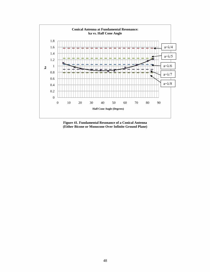
6. SUMMARY

Theoretical analysis of the fundamental resonant frequency and radiation

characteristics of a wide-angle, conical antenna as a function of half cone angle

and slant height has a high degree of complexity. Analysis is based on treating the

conical structure as a transmission line and evaluating the terminating admittance

by determining characteristic solutions to Maxwell’s equations and applying

relevant boundary conditions. Including just a single TEM mode (and neglecting

all others modes) simplifies the problem but leads to significant error in the

prediction of the fundamental resonance of a conical antenna when compared to

results of simulation and experiment. Sufficient improvements to the theory are

obtained by including just a few higher order terms; however this greatly

increases the complexity of the equations.

The results of experiment obtained from the literature, numerical simulation with

CST MWS and the second order approximation to the Schelkunoff mode theory

of antennas derived by P.D.P. Smith are all in good agreement. Experiments

conducted by the author (J.E. Lawrance) also yielded results that were consistent

with these findings. The fundamental resonant frequency of a conical antenna as a

function of half cone angle is presented in the graph of Figure 41. Fundamental

resonance occurs at a significantly lower value than one might expect for large

half cone angles.

In addition, while the radiation efficiency of a conical antenna is maximum at a

45° half cone angle, the peak electric field in the far zone increases with

increasing half cone angle for a constant charge voltage. This is because, for a

fixed charge voltage, the antenna capacitance (and therefore the total stored

energy) increases as the half cone angle is increased.

48

Figure 41. Fundamental Resonance of a Conical Antenna

(Either Bicone or Monocone Over Infinite Ground Plane)

0

0.2

0.4

0.6

0.8

1

1.2

1.4

1.6

1.8

0 10 20 30 40 50 60 70 80 90

ka

Half Cone Angle (Degrees)

Conical Antenna at Fundamental Resonance:

ka vs. Half Cone Angle

a=λ/4

a=λ/7

a=λ/5

a=λ/6

a=λ/8

49

7. CONCLUSION

The self resonant bicone antenna is a useful radiator for compact pulse power

systems due to its relatively small size, its suitability to high voltage

environments, and its broadband radiation characteristics. In this application, the

center frequency and peak amplitude of the radiated pulse will depend on the half

cone angle and cone slant height. In order to maximize stored energy, large half

cone angles are employed in the antenna design.

It is commonly assumed that the relationship between slant height and the

wavelength λ at the fundamental resonant frequency corresponds to λ/4, with

some relatively minor correction for end effects. The results presented herein

establish that this is inaccurate for large half cone angles (i.e., α > 5°) and that in

fact this relationship approaches λ/8.

The gain and radiation pattern of this antenna are similar to that of a dipole of the

same length, as is the case for all electrically small antennas.

If maximizing peak electric field at a fixed distance is desirable – for a fixed

charge voltage – the broader the half cone angle the better. If instead it is desired

to maximize energy radiated along the equator, the optimum half cone angle is

45°.

While most of the theoretical derivations, numerical simulations and experiments

presented in this paper were conducted for a monocone over an an infinite

groundplane, the results are directly applicable to a bicone. For practical

applications, a monocone over a groundplane would not suffice because the

groundplane would have to be unacceptably large to appear infinite. For practical

applications it is preferable to employ a bicone in order to keep the overall

dimensions of the antenna small.

50

8. REFERENCES

1. C.A. Balanis, Antenna Theory, 3rd

Edition, Wiley and Sons, 2005, p. 500-504

2. C.E. Baum, “A Circular Conical Antenna Simulator”, Sensor and Simulation

Notes, Note 36, March 1967

3. S.A. Schelkunoff, Advanced Antenna Theory, Wiley and Sons, 1952

4. S.A. Schelkunoff, “General Theory of Symmetric Biconical Antennas”, Journal of

Applied Physics, Vol. 22, Number 11, Nov. 1951

5. C. H. Papas and R.W.P. King, “Input Impedance of Wide Angle Conical

Antennas Fed By a Coaxial Line”, Proc. I.R.E. , Vol. 39, pp. 1269, Nov 1949

6. C.H. Papas and R.W.P. King, “Radiation from Wide-Angle Conical Antennas Fed

by a Coaxial Line”, Proc. I.R.E., Vol. 39, pp. 49, Jan 1951

7. P.D.P. Smith, “The Conical Dipole of Wide Angle,” Jour. Appl. Phys., vol.19, pp.

11-23; January, 1948

8. P.D.P. Smith, “Ground Plane Field of the Wide Angle Conical Dipole”, Jour.

Appl. Phys., vol. 20, p. 636

9. S.A. Schelkunoff, “Principal and Complementary Waves in Antennas”,

Proceedings of the I.R.E, January, 1946, pp. 23-31

10. G.H. Brown and O.M. Woodward, “Experimentally Determined Radiation

Characteristics of Conical and Triangular Antennas, RCA Review, Vol. 13, pp.

425-452, December, 1952

11. Designed by C. Jerald Buchenauer ca. 1998.

12. S. A. Schelkunoff, “Theory of Antennas of Arbitrary Size and Shape”, Proc.

I.R.E., vol 29, pp. 493-521, April 1941

13. C.T. Tai, “Application of a Variational Principle to Biconical Antennas, Jour.

Appl. Phys., vol. 20, pp. 1076-1084, 1948

14. J.A. Stratton and Chu, “Forced Oscillations of a Cylindrical Conductor”, Journal

of Applied Physics, vol. 12., pp. 230-240 (1941)

15. J.A. Stratton and Chu, “Forced Oscillations of a Prolate Spheroid”, Journal of

Applied Physics, vol. 12., pp. 241-248 (1941)

51

16. D. N. Black and T. A. Brunasso, “An Ultra Wideband Bicone Antenna”, Ultra-

Wideband, IEEE International Conference on Ultra-Wideband, 2006, 15 January,

2007

17. C.W. Harrison, Jr. and C.S. Williams, Jr., “Transients in Wide-Angle Conical

Antennas”, IEEE Trans. AP13, pp. 236-246, 1965

18. M. Armanious, J.S. Tyo, M.C. Skipper, M.D Abdalla, W.D. Prather and J.E.

Lawrance, “IEEE Trans. PS38, pp. 1124-1131, May 2010

19. C.T. Tai, “On the Theory of Biconical Antennas”, Jour. Appl. Phys., vol. , pp.

1155-1160, Dec. 1948

20. C.A. Balanis, Antenna Theory, 3rd

Edition, Wiley and Sons, 2005, p. 510

52

Appendix A. Matlab Program to Evaluate Input Impedance from Theory

clear

alpha=30;

a=alpha*pi/180;

x=cos(a);

Z0=60*log(cot(a/2));

i=(-1)^.5;

ka=.1:.1:10;

zero=0*ka;

Zc=Z0+0*ka;

f0=besselj(0,ka);

f1=besselj(1,ka);

f2=besselj(2,ka);

f3=besselj(3,ka);

f4=besselj(4,ka);

f5=besselj(5,ka);

f6=besselj(6,ka);

f7=besselj(7,ka);

f8=besselj(8,ka);

f9=besselj(9,ka);

f10=besselj(10,ka);

f11=besselj(11,ka);

f12=besselj(12,ka);

f13=besselj(13,ka);

f14=besselj(14,ka);

f15=besselj(15,ka);

f16=besselj(16,ka);

f17=besselj(17,ka);

f18=besselj(18,ka);

f19=besselj(19,ka);

f20=besselj(20,ka);

f21=besselj(21,ka);

g0=bessely(0,ka);

g1=bessely(1,ka);

g2=bessely(2,ka);

g3=bessely(3,ka);

g4=bessely(4,ka);

g5=bessely(5,ka);

g6=bessely(6,ka);

g7=bessely(7,ka);

g8=bessely(8,ka);

g9=bessely(9,ka);

g10=bessely(10,ka);

g11=bessely(11,ka);

g12=bessely(12,ka);

g13=bessely(13,ka);

g14=bessely(14,ka);

g15=bessely(15,ka);

g16=bessely(16,ka);

g17=bessely(17,ka);

g18=bessely(18,ka);

g19=bessely(19,ka);

g20=bessely(20,ka);

g21=bessely(21,ka);

h0=f0-i*g0;

h1=f1-i*g1;

h2=f2-i*g2;

h3=f3-i*g3;

53

h4=f4-i*g4;

h5=f5-i*g5;

h6=f6-i*g6;

h7=f7-i*g7;

h8=f8-i*g8;

h9=f9-i*g9;

h10=f10-i*g10;

h11=f11-i*g11;

h12=f12-i*g12;

h13=f13-i*g13;

h14=f14-i*g14;

h15=f15-i*g15;

h16=f16-i*g16;

h17=f17-i*g17;

h18=f18-i*g18;

h19=f19-i*g19;

h20=f20-i*g20;

h21=f21-i*g21;

zeta1=h1./(h0-(3./ka).*h1);

zeta3=h3./(h2-(3./ka).*h3);

zeta5=h5./(h4-(5./ka).*h5);

zeta7=h7./(h6-(7./ka).*h7);

zeta9=h9./(h8-(9./ka).*h9);

zeta11=h11./(h10-(11./ka).*h11);

zeta13=h13./(h12-(13./ka).*h13);

zeta15=h15./(h14-(15./ka).*h15);

zeta17=h17./(h16-(17./ka).*h17);

zeta19=h19./(h18-(19./ka).*h19);

zeta21=h21./(h20-(21./ka).*h21);

P1=mfun('P',1,x);

P3=mfun('P',3,x);

P5=mfun('P',5,x);

P7=mfun('P',7,x);

P9=mfun('P',9,x);

P11=mfun('P',11,x);

P13=mfun('P',13,x);

P15=mfun('P',15,x);

P17=mfun('P',17,x);

P19=mfun('P',19,x);

P21=mfun('P',21,x);

prod1=((2*1+1)/(1*(1+1)))*P1^2.*zeta1;

prod3=((2*3+1)/(3*(3+1)))*P3^2.*zeta3;

prod5=((2*5+1)/(5*(5+1)))*P5^2.*zeta5;

prod7=((2*7+1)/(7*(7+1)))*P7^2.*zeta7;

prod9=((2*9+1)/(9*(9+1)))*P9^2.*zeta9;

prod11=((2*11+1)/(11*(11+1)))*P11^2.*zeta11;

prod13=((2*13+1)/(13*(13+1)))*P13^2.*zeta13;

prod15=((2*15+1)/(15*(15+1)))*P15^2.*zeta15;

prod17=((2*17+1)/(17*(17+1)))*P17^2.*zeta17;

prod19=((2*19+1)/(19*(19+1)))*P19^2.*zeta19;

prod21=((2*21+1)/(21*(21+1)))*P21^2.*zeta21;

Sum=prod1+prod3+prod5+prod7+prod9+prod11+prod13+prod15+prod17+prod19+prod

21;

ratio=(1+i*(60/Z0).*Sum)./(-1+i*(60/Z0).*Sum).*exp(-2*i*ka);

Zin=Z0*(-2*ratio)./(1+ratio);

figure (1)

plot(ka,[imag(Zin);zero])

figure (2)

plot(ka,[real(Zin);Zc])

54

Appendix B: Effect of Finite Ground Plane (Simulation with CST

Microwave Studio)

The effect of a finite ground plane was briefly explored in simulations with CST

Microwave Studio. The half cone angle was kept constant at 5° and the slant

height of the cone was also kept constant at 0.3m. The ground plane was a 1mm

thick circular disc in the x-z plane as illustrated in Figure 42. The radius of the

ground plane ranged from 0.3 meters to 1.2 meters in 0.3 meter increments.

Figure 42. Hollow Cone Over Finite Ground Plane (ground plane radius = 0.3m)

The vertically polarized electric field measured in this simulation for a ground

plane radius of 0.3m at a distance of 5m along a radial axis is shown in Figure 43.

For this configuration, it was found that the peak field was close to that for an

infinite ground plane (at about 0.03V/m); however the resonant frequency was

found to be higher (at 186MHz, compared to 175 MHz observed with an infinite

gound plane).

Figure 43. Radiated Electric Field, Finite Ground Plane

55

The results can best be seen in the three dimensional plots of the radiation pattern

as the radius of the ground plane is increased. These are presented in Figures 44-

47.

Figure 44. Ground Plane Radius = 0.3 meters.

Figure 45. Ground Plane Radius = 0.6 meters

Figure 46. Ground Plane Radius = 0.9 meters

Figure 47. Ground Plane Radius = 1.2m

56

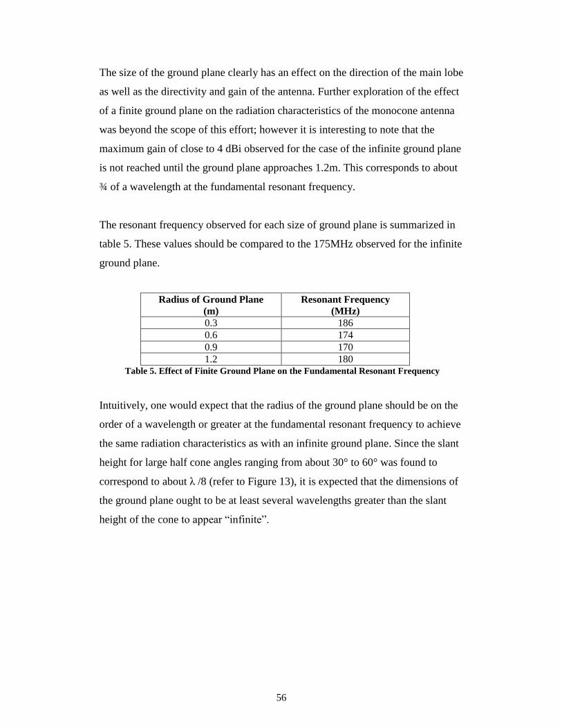
The size of the ground plane clearly has an effect on the direction of the main lobe

as well as the directivity and gain of the antenna. Further exploration of the effect

of a finite ground plane on the radiation characteristics of the monocone antenna

was beyond the scope of this effort; however it is interesting to note that the

maximum gain of close to 4 dBi observed for the case of the infinite ground plane

is not reached until the ground plane approaches 1.2m. This corresponds to about

¾ of a wavelength at the fundamental resonant frequency.

The resonant frequency observed for each size of ground plane is summarized in

table 5. These values should be compared to the 175MHz observed for the infinite

ground plane.

Radius of Ground Plane

(m)

Resonant Frequency

(MHz)

0.3 186

0.6 174

0.9 170

1.2 180 Table 5. Effect of Finite Ground Plane on the Fundamental Resonant Frequency

Intuitively, one would expect that the radius of the ground plane should be on the

order of a wavelength or greater at the fundamental resonant frequency to achieve

the same radiation characteristics as with an infinite ground plane. Since the slant

height for large half cone angles ranging from about 30° to 60° was found to

correspond to about λ /8 (refer to Figure 13), it is expected that the dimensions of

the ground plane ought to be at least several wavelengths greater than the slant

height of the cone to appear “infinite”.

57

Appendix C: Resonant Frequency and Radiation Characteristics of

Bicone Antenna

The fundamental resonant frequency and radiation characteristics of a bicone

antenna with the same slant height as the monocone antenna used in simulations

in Section 3 was also explored briefly. The 30° hollow bicone is shown in Figure

48.

Figure 48. 30° Bicone Antenna (Slant Height = 0.3 m)

The measured electric field along the radial axis at 5m for this structure is shown

in Figure 49. The resonant frequency was found to be 139.9 MHz, identical to that

observed in simulations for the monocone over an infinite ground plane; however

the peak field was one-half that measured for the monocone.

Figure 49. Radiated Pulse for Bicone with 30° Half Cone Angle

58

The radiation pattern for the bicone with 30° half cone angle is shown in Figure 50. It

was similar to that observed for the monocone antenna; however it was a full toroid

rather than the half toroid pattern observed for the monocone structure (compare to

Figure 28).

Figure 50. Radiation Pattern for a 30° Bicone Antenna

The main lobe beamwidth was therefore found to be twice that for the monocone with the

same slant height and half cone angle, as shown in Figure 51.

Figure 51. Polar Plot of Radiation Pattern

Simulations were run for bicone antennas with a slant height of 0.3 meters and half cone

angles of 30° and 60°. The fundamental resonant frequencies were determined to be

identical to those found for the monocone structures over an infinite ground plane with

the same slant height and half cone angle, as expected.