The Full Costs of Thermal Power Production in Eastern Canada Henry David Venema Stephan Barg July 2003

This document was produced as part of the India-Canada Energy Efficiency project. The partners in this project are The Energy and Resources Institute (http://www.teriin.org), the International Institute for Sustainable Development (http://www.iisd.org/) and the Pembina Institute for Alternative Development (http://www.pembina.org/). This project is undertaken with the financial support of the Government of Canada provided through the Canadian International Development Agency. This report documents research conducted collaboratively with The Energy and Resources Institute and is intended to foster North-South collaboration and institutional capacity on energy and climate policy issues of mutual importance. The International Institute for Sustainable Development contributes to sustainable development by advancing policy recommendations on international trade and investment, economic policy, climate change, measurement and indicators, and natural resources management. By using Internet communications, we report on international negotiations and broker knowledge gained through collaborative projects with global partners, resulting in more rigorous research, capacity building in developing countries and better dialogue between North and South.

IISD’s vision is better living for all—sustainably; its mission is to champion innovation, enabling societies to live sustainably. IISD receives operating grant support from the Government of Canada, provided through the Canadian International Development Agency (CIDA) and Environment Canada, and from the Province of Manitoba. The institute receives project funding from the Government of Canada, the Province of Manitoba, other national governments, United Nations agencies, foundations and the private sector. IISD is registered as a charitable organization in Canada and has 501(c)(3) status in the United States.

Copyright © 2003 International Institute for Sustainable Development

Published by the International Institute for Sustainable Development

All rights reserved International Institute for Sustainable Development 161 Portage Avenue East, 6th Floor Winnipeg, Manitoba, Canada R3B 0Y4 Tel: +1 (204) 958-7700 Fax: +1 (204) 958-7710 E-mail: info@iisd.ca Web site: http://www.iisd.org/

Table of Contents

Executive Summary...................................................................................................................................... 1

1 Introduction....................................................................................................................................... 10 1.1 Motivation ................................................................................................................................. 10 1.2 The Canadian Power Sector at a Glance................................................................................. 12 1.3 Calculating Externalities: Theory and Practice ...................................................................... 13

2 The State of the Art: ExternE.......................................................................................................... 16 2.1 Impact-Pathway Methodology ................................................................................................. 16 2.2 Representative ExternE Results ............................................................................................... 18

3 Externalities Research in Canada.................................................................................................... 20

4 Estimating Power Sector Externalities in Canada ......................................................................... 24 4.1 Air Pollution Externalities Overview ....................................................................................... 24

4.1.1 Source-Receptor Model for SO4 and SO2............................................................................. 28 4.1.2 Source-Receptor Model for O3 ............................................................................................. 34 4.1.3 Air Pollution Damages Estimation using AQVM................................................................. 39

4.2 Greenhouse Gas Externalities.................................................................................................. 46 4.2.2 GHG Inventory Analysis ...................................................................................................... 49 4.2.3 Climate Change Damages Estimation .................................................................................. 52

4.3 Aggregate Externalities and Uncertainty Analysis.................................................................. 55 4.4 Sources of Uncertainty and Biases .......................................................................................... 57

5 Policy Implications............................................................................................................................ 58 5.1 Kyoto Compliance..................................................................................................................... 58

6 Conclusions........................................................................................................................................ 61

References ................................................................................................................................................... 62

1

Executive Summary

Introduction The economic or financial cost of a product is often not its full cost because environmental costs are typically neglected. These costs constitute a loss of social welfare due to their negative human health and ecological impacts, and are usually referred to as externalities, because they are considered external to the market price for a product. For example, burning fossil fuels like coal or gasoline creates air pollution, which can damage the health of people who breathe the air. The full cost of this health damage is rarely if ever counted in the price of the goods or services produced when the coal or gasoline is burned, but the cost is nevertheless borne by individuals and society as a whole. Full cost accounting quantifies the economic cost of such externalities. Buyers of gasoline or coal-based electricity therefore pay less than its real cost, and are inclined to use more of it than they otherwise would. Wherever prices of goods or services do not reflect full costs, markets are distorted and society bears the burden of this loss of social welfare. Government regulators frequently attempt to reduce social welfare losses by imposing emission restrictions, but these limits are typically set with respect to estimates of permissible exposure levels, and for many critical pollutants any exposure level is damaging. Unlike financial accounting, full cost accounting can never be precise; the science that links pollution emissions to all their human, material and environmental impacts is incomplete. We simply do not understand all the ways in which pollutants interfere with the proper functioning of our bodies, our infrastructure and the ecosystems that sustain us. Even in cases where we think we understand the direct impacts of pollutants, calculating the economic cost requires people to place a value on their willingness to avoid exposure to the pollutant, and the increased risk to their health posed that exposure poses. Environmental costs remain highly uncertain, although research in techniques for valuating the economic worth of the services that ecosystems provide may, in time, reduce these uncertainties. Despite such fundamental uncertainties, the science and methods for full cost accounting have advanced considerably in recent decades and allow us to make conservative estimates of the magnitudes of some types of externalities. This study uses the available data and analytical approaches to develop estimates for the cost of externalities arising from electricity generation using coal, oil or natural gas in Eastern Canada. The sector is chosen for three related reasons: it is a large emitter of air pollutants and greenhouse gases; it will undergo potentially significant structural changes as Canada complies with the Kyoto Protocol; and alternative investments in non-polluting sources of electricity should include analysis of full costs. Two broad types of externalities are evaluated in this study—the public health costs caused by emissions of sulphur and nitrogen oxides (SOx and NOx) and volatile organic carbon (VOC) in Eastern Canada, and the marginal climate change damages caused by the emissions of

2

greenhouse gasses (GHGs) in Eastern Canada. The data, atmospheric models and costing models that underlie this analysis are largely from Canadian federal government sources. Tables E.1 and E.2 indicate the magnitude of the air pollution and GHG emissions from the thermal power sector, and relative to the national total. This study examined the economic costs associated with SOx, NOx, VOC and GHG emissions from thermal power generation. SOx emissions from thermal power plants react in the atmosphere producing sulphate aerosols (SO4) and sulphur dioxide (SO2), with negative human health and material damage impacts. NOx and VOC react to produce ground-level ozone (O3), which also has a range of negative human health impacts. Thermal power generation (primarily coal) also produces toxic emissions such as mercury, arsenic, dioxins, furans and lead, however the methodology for quantifying the impacts of air toxins is not developed to the point where we could include them in this study.

Table E.1 1995 Selected Criteria Air Contaminants (1995)1 SOX NOX VOC

Electric Power Generation 534,323 254,985 2,980

National Total 2,653,571 2,463,971 3,575,202

Power Sector Percentage 20.14% 10.35% 0.08%

Source: http://www.ecgc.ca/pdb/ape/cape_home_e.cfm

Table E.2 Canadian Power Sector Greenhouse Gas Emissions (kt CO2-eq)

1995 1996 1997 1998 1999 2000

Electricity & Heat Generation

101,000 99,700 111,000 124,000 121,000 128,000

Total 658,000 672,000 682,000 689,000 703,000 726,000

Power Sector Percentage 15.35% 14.84% 16.28% 18.00% 17.21% 17.63%

Source: http://www.ec.gc.ca/pdb/ghg/documents/Gasinventory2000.pdf

The Impact-Pathway Approach for Air Pollutants The major contribution of this study is the application of the impact-pathway approach to the power sector emissions. Recent Canadian studies have reported either the pollutant emission rates for different power generation technologies and fuels, or the health costs of ambient air pollution—not specifically attributable to the power sector. This study isolates the component of air pollution attributable to the power sector and analyses its geographic distribution. Our approach is adapted from two primary sources; ExternE, a large European Commission research project to standardize methods for quantifying power sector externalities in 15 EU countries, and a Canadian study conducted by the 1 The 1995 Criteria Air Contaminant Emissions for Canada (CAPE) database [Environment Canada, 1998] is the most comprehensive government database of air contaminant emissions. The Criteria Air Contaminants are: Total Particulate Matter (TPM), Particulate Matter ≤ 10 microns (PM10), Particulate Matter ≤ 2.5 microns (PM2.5), Sulphur Oxides (SOX), Nitrogen Oxides (NOX), Volatile Organic Compounds (VOC), Carbon Monoxide (CO)

3

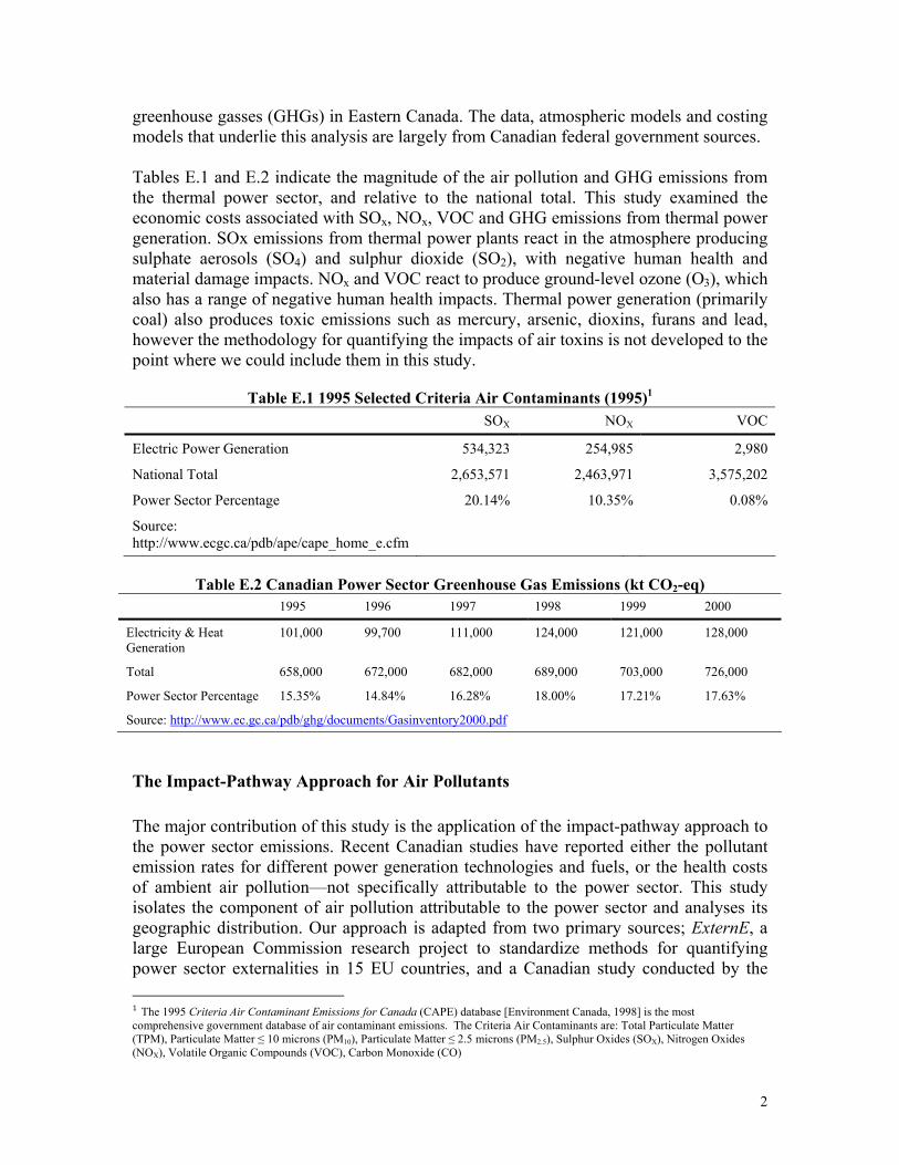
Analysis and Modelling Group (AMG) as part of the National Climate Change Process, The Environmental and Health Co-benefits of Actions to Mitigate Climate Change. ExternE provided the basic conceptual framework for characterizing the emissions, dispersion, impact and cost quantification of air pollutants from the power sector and is shown conceptually in Figure E.1. We adapted the emission-dispersion modelling (steps 1 and 2 of the impact-pathway approach) from earlier studies done for the AMG and calculated the average SO4 and SO2 concentrations in individual Census divisions in Eastern Canada. Unfortunately no comparable air pollution modelling studies exist for Western Canada and our analysis applies only to Ontario, Quebec and the Maritime provinces. We isolated the increment of air pollution attributable to the power sector by using linear proportionality principles previously applied by the AMG. Figures E.2 and E.4 show maps of the average annual SO4 and SO2 concentrations attributable to the power sector. The computational effort required to model the dispersion of emissions from multiple individual power plants is not currently feasible, therefore the impact-pathway analysis attributes damages to the Eastern Canadian power sector as a whole, and not to individual plants. We also developed an impact-pathway model to calculate the ozone concentrations attributable to the power sector within individual Census divisions. The ozone model used monitored ozone data from the National Air Pollution System (NAPS and related the incremental ozone concentration to the increment of NOx and VOC emissions from the power sector.

Figure E.1 The impact-pathway approach.

4

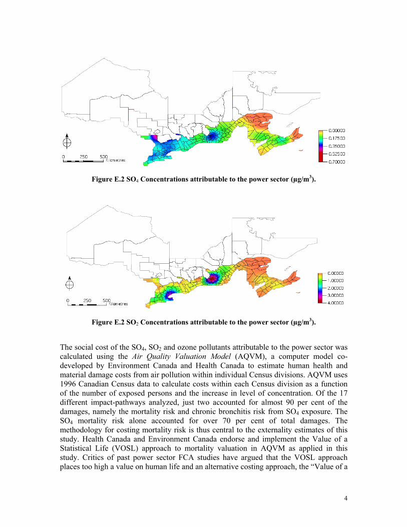
Figure E.2 SO4 Concentrations attributable to the power sector (µg/m3).

Figure E.2 SO2 Concentrations attributable to the power sector (µg/m3). The social cost of the SO4, SO2 and ozone pollutants attributable to the power sector was calculated using the Air Quality Valuation Model (AQVM), a computer model co-developed by Environment Canada and Health Canada to estimate human health and material damage costs from air pollution within individual Census divisions. AQVM uses 1996 Canadian Census data to calculate costs within each Census division as a function of the number of exposed persons and the increase in level of concentration. Of the 17 different impact-pathways analyzed, just two accounted for almost 90 per cent of the damages, namely the mortality risk and chronic bronchitis risk from SO4 exposure. The SO4 mortality risk alone accounted for over 70 per cent of total damages. The methodology for costing mortality risk is thus central to the externality estimates of this study. Health Canada and Environment Canada endorse and implement the Value of a Statistical Life (VOSL) approach to mortality valuation in AQVM as applied in this study. Critics of past power sector FCA studies have argued that the VOSL approach places too high a value on human life and an alternative costing approach, the “Value of a

5

Life Year Lost” (VOLY), which generally produces lower mortality cost estimates, should instead be used. However at the time of this study (December 2002), Health Canada and Environment Canada maintained that the VOLY approach is not sufficiently well-supported in the scientific literature to justify its use. The total public health externalities estimated for all SO4, SO2 and O3 impact-pathways were then attributed to individual fuels used for power generation on the basis of their relative emission rates of precursors to the formation of SO4, SO2 and O3, namely SOX, NOX and VOCs. Figure E.4 illustrates the central estimate and uncertainty bounds (one standard deviation) for the public health externalities by fuel type and reveals the high public health externality cost of coal. Two factors explain coal’s high public health cost: the overwhelming dominance of SO4 mortality risk among the various impact-pathways, and the high SOx emissions rate for coal-fired power compared to other fuels. The public health cost for gas is underestimated because it does create large SOx emissions, but in upstream production stages (not accounted for in this study) and not at the point of combustion.

$0.0171

$0.0038

$0.0001

$0.000

$0.005

$0.010

$0.015

$0.020

$0.025

$0.030

$0.035

COAL GAS OIL Figure E.4 Thermal power air quality externalities in Canada ($/kWh).

Global Warming Global warming damages from GHG emissions constitute the other major externality category evaluated in this study. GHG externalities include the negative effects of global warming on health, agriculture, water supply, sea level rise, ecosystems and biodiversity. The key principle underlying the integrated assessment of global warming is that the location of GHG emissions is irrelevant to the marginal damages they cause since GHGs

6

mix completely with other gas in the atmosphere soon after they are emitted. We could therefore utilize the results of previous studies that have linked General Circulation Models (GCMs) that predict the future climate as a function of atmospheric GHG concentrations, with Integrated Assessment Models (IAMs) that quantify the impacts of the future climate. Quantifying the marginal cost of GHGs is dependent on many assumptions about how impacts are valued, not only in Canada, but globally since, at the margin, a unit of GHG emissions in Canada or anywhere else in the world is equally responsible for impacts everywhere in the world. We therefore based the marginal GHG damage estimate used in this study on the globally averaged valuation of impacts. Our central estimate is $26/tonne CO2-eq, which is in the lower range of published values. This number is the (Canadian dollar) amount developed for the ExternE damage estimates. As a comparison, the Government of Canada currently assumes GHG purchase prices in the range of $10–$15/tonne CO2-eq on the international market. Figure E.5 shows the central estimate and uncertainty bounds (one standard deviation) for global warming externalities for coal, gas and oil-fired power generation in Canada, which are differentiated on the basis of their relative GHG emissions intensity.

0.0223

0.0180

0.0101

$0.000

$0.005

$0.010

$0.015

$0.020

$0.025

$0.030

$0.035

$0.040

COAL GAS OIL

Figure E.5 Thermal power global warming externalities in Canada ($/kWh).

Thermal Power Sector Aggregate Externalities and Uncertainties Figure E.6 shows our central estimate and uncertainty bounds for the aggregate air quality and global warming externalities attributable to the thermal power sector in Eastern Canada. Our estimates are approximately half those of a similar ExternE study in the U.K. The differences can be explained in part by the lower population density in Eastern Canada and hence lower total exposure to air pollutants emitted by the power sector.

7

The results of this study can be considered a conservative first estimate as a large number of known impacts could not be evaluated because neither the data nor the damage function were available. The known but unquantified uncertainties and systematic analytical biases, as well as an assessment of how their omission has biased our central estimates are included below.

Fundamental Uncertainties (damage functions known to exist but data not available)

• Carbon monoxide causing cardiac hospital admissions (bias downward) • Acid deposition impacting fishing yields (bias downward) • Air toxins and risks of cancers, neurological disorders (bias downward) • Ozone damages on agricultural crops (bias downward)

Fundamental Uncertainties (damage functions unknown but believed to exist)

• NOx emissions impacts on agriculture and ecosystems (bias downward) • Air toxics impacts on terrestrial wildlife (bias downward) • Acid deposition impacts on ecosystems (bias downward)

Systematic Analytical Biases

• Power production statistics are not perfectly aligned with 1995–1998 air emissions data; (bias downward with respect to total externalities, unknown with respect to unit externalities).

• 17 per cent systematic under-estimate of GHG emissions (bias downward) • No air quality externalities in Western Canada (bias downward) • No air quality externalities from Eastern Canadian

sources with U.S. receptors (bias downward) • Atmospheric transport mechanisms (bias unknown) • No upstream source-receptor model for gas (bias downward) • GHG costs a subset of unknown size of all impacts (bias downward) • Mortality valuation methodology (bias unknown, probably upward)

8

$0.0218

$0.0394

$0.0102

$0.000

$0.010

$0.020

$0.030

$0.040

$0.050

$0.060

$0.070

COAL GAS OIL

Figure E.6 Thermal power aggregate externalities in Canada ($/kWh).

Policy Implications and Conclusions Canadian thermal power sector externalities cannot be known exactly, however they are clearly non-zero. The fundamental policy implication is that if Canadian thermal power producers had to internalize externalities, their emissions would decrease because it would be economically sound to do so. Reducing emissions from coal-fired power generation should be a particularly important policy objective. The central estimate of coal externalities from this study ($0.0394/kWh) is about 50 per cent higher than the marginal cost of production of electricity from coal (~$0.026/kWh). Excluding global warming damages, the central estimate of the public health externalities alone ($0.0171/kWh) is about 65 per cent of the marginal production cost. Electricity prices for power generated by natural gas are significantly less distorted by the failure to internalize externalities. Our central estimate for gas externalities ($0.0102/kWh) is approximately 20 per cent of the estimated marginal production cost. Public health externalities for gas are negligible—about 0.2 per cent of the marginal production cost (not including externalities from upstream gas production and distribution). Canada’s recent Kyoto ratification provides new impetus for revisiting the mix of generation technologies within the Canadian power sector. The Government of Canada’s Climate Change Action Plan [Government of Canada, 2003], Canada’s nascent strategy for Kyoto compliance, provides illustrative examples of the expected price signal seen by different economic sectors under the current federal plan for Kyoto compliance. Coal-fired power production will see a price increment of about 1.94 per cent of the wholesale cost of production under the federal plan. A fundamental concern is that the thrust of the federal strategy is to ensure that the price signal seen by large emitters (including coal-

9

fired power generators) will be small enough so that appropriate levels of emission reductions may not be realized. The federal government bears a risk that it must purchase emissions reduction credits on international markets to achieve the national target which, in the case of coal-fired power, means that Canada will also be forgoing the domestic air quality co-benefits of domestic action to curb emissions. We examine how the explicit inclusion of externalities would influence power sector investment decision-making with an example based on the Nanticoke coal-fired power plant in southern Ontario. While this example is included for illustrative purposes it does demonstrate how alternative energy strategies based on demand side management and large-scale renewable energy are typically under-valued because the clean air and climate change mitigation co-benefits are not included in the economic analysis. By providing defensible, conservative estimates of the full costs of energy production, this study helps clarify how Canada can achieve significant public health and climate change mitigation co-benefits by decreasing reliance on conventional coal-based power.

10

1 Introduction This study provides an estimate of the public health and global warming costs associated with fossil fuel combustion in the Canadian thermal power sector. Externalities costing exercises such as this are also known as Full Cost Accounting or simply FCA. The study is organized around the following components:

• The policy rationale for estimating environmental externalities in general, and with respect to the power sector specifically (sections 1.1 and 1.2).

• The theoretical rational for estimating externalities and a review of early attempts at estimating power sector externalities (sections 1.3).

• A review of the current state of the art in power sector FCA focusing on source-receptor modelling and the impact-pathway approach (section 2).

• A review of externalities research in Canada (section 3). • The methodology developed at IISD for FCA of the Canadian thermal power

sector (section 4), including specifically: o relevant air quality research in Canada (section 4.1) o the development of source-receptor models for the following air

pollutants: SO4, SO2 and O3 (sections 4.1.1 and 4.1.2); o the public health costs of exposure to ambient SO4, SO2 and O3

attributable to power sector air pollution emissions (sections 4.1.3); o attribution of the public health costs to the major thermal power fuel types:

coal, oil and gas (section 4.1.4); o the standard methodology for estimating global warming externalities

from greenhouse gas emissions (section 4.2.1); o a greenhouse gas emissions inventory analysis for the Canadian thermal

power sector (section 4.2.2); o calculation of global warming damages attributable to the Canadian

thermal power sector (section 4.2.3); and o synthesis of aggregate public health and global warming externalities,

including an analysis of uncertainty (sections 4.3 and 4.4). • A discussion of the implications of FCA in the Canadian power sector in the

broad context of Kyoto compliance and in the specific context of power sector investment decision-making using an illustrative example (section 5).

• Conclusions (section 6).

1. 1 Motivation A key research element of the Green Budget Reform component of the TERI-Canada Energy Efficiency Project is full cost accounting (FCA) of electricity production in India and Canada. The essential thrust of Green Budget Reform is to inform policy-makers about the real cost of production—costs that include environmental externalities.

11

Although the concept of externalities has been firmly ensconced theoretical welfare economics since Pigou [1932] [Ayres and Kneese, 1969], attempts to rigorously apply it in policy-making have only gained prominence more recently. Parties to the United Nations Conference on Environment and Development (UNCED), convened in Rio de Janeiro in 1992 for the Earth Summit and agreed to a set of environmental governance principles, known as Agenda 21, Principle 16 of which states that:

National authorities should endeavor to promote the internalization of environmental costs and the use of economic instruments, taking into account the approach that the polluter should, in principle, bear the cost of pollution, with due regard to the public interest and without distorting international trade and investment.

The central thrust of the European Commission’s Fifth Environmental Action Programme, “Towards Sustainability,” in the 1990s was the integration of the best possible scientific and technical information on environmental externalities within the decision-making process in non-environmental policy areas [Krewitt, 2002]. If externalities are not known or cannot be known exactly, “the traditional economic goal of welfare optimization is a chimera” [EC, 1996]. Much of the existing technical research on environmental externalities has focused on the energy sector and particularly electricity production, primarily because of its economic significance and the large pollutant emissions associated with thermal power generation. The North American Commission for Environmental Cooperation (NACEC) reports, for example, that the U.S. and Canada are among the highest air polluters in the world, “chief among the reasons for this is the fact that these two countries are the highest per capita consumers of fossil fuels”[CEC, 2001, p62]. The electric power sector is a very large consumer of those fossil fuels, indeed. NACEC also reports that North American power plants recorded the largest toxic releases in 1999 among all reporting industrial sectors—more than 450,000 tonnes of pollutant emissions to air, land and water [CEC, 2001].

Clarifying the full costs of power generation for regulators and policy-makers is particularly critical given the large investment requirements in the power sector and the potential shifts in the structure of the power sector. NAFTA governments project that the demand for electricity will grow by 14 per cent in Canada, 66 per cent in Mexico, and 21 per cent in the United States from 2000 to 2009 [CEC, 2002a]. The need for full cost accounting in the power sector is particularly acute because of the non-differentiation in prices among electricity supplies generated from different sources with potentially very different pollution emissions and externalities. Full cost accounting quantifies the environmental externalities associated with electricity production. The basic objective is to make explicit the magnitude of direct environmental costs borne by society from electricity production—thereby influencing decision-makers towards power sector investment decisions that are indeed least cost. In the Canadian context, the power sector FCA exercise also helps illuminate the rationale for Canada’s

12

ratification of the Kyoto Protocol, which compels Canada to curb greenhouse gas emissions including, notably, from the power sector. This study provides a significantly improved estimation of the public health costs associated with thermal power production. The study provides estimates of the domestic co-benefits forgone if emissions reduction credits are purchased on the international market rather than reducing emissions from the domestic power sector. Although the purchase of emissions reduction credits may be the least-cost option in financial terms, if the socio-economic burden of power sector externalities is also considered, the least-cost option in many cases will be to reduce domestic emissions by displacing with lower emissions fuels or through demand side management and/or renewable energy. We anticipate that FCA principles and externalities will be increasingly important considerations as Canada implements its Kyoto compliance strategy.

1.2 The Canadian Power Sector at a Glance The Canadian power sector is dominated by hydropower, but includes substantial amounts of thermal and nuclear power generation. The proportion of non-conventional renewable energy, such as wind and biomass is also increasing. Thermal power (coal, oil and natural gas-fired electrical generation) dominates in the Maritimes, Alberta and Saskatchewan and is a large power supplier in Ontario. Table 1 shows the annual power generation by fuel source [NEB, 1999]. Tables 2 and 3 list the total emissions of greenhouse gasses [Environment Canada, 2001b] and criteria air pollutants from the power sector [Environment Canada, 1998].2

Table 1 1997 Canadian electricity generation by technology and fuel type.

Coal Oil Gas Nuclear Hydro Wind Biomass

Total Generation (GWH) 91,283 9,210 23,963 77,963 341,951 45 6,719

Percentage of Total 16.56% 1.67% 4.35% 14.15% 62.04% 0.01% 1.22%

Source: National Energy Board (1999) Canadian Energy Supply and Demand to 2025 Table A4.1a

Table 2

Canadian power sector greenhouse gas emissions (kt CO2-eq). 1995 1996 1997 1998 1999 2000

Electricity and Heat Generation

101,000 99,700 111,000 124,000 121,000 128,000

Total 658,000 672,000 682,000 689,000 703,000 726,000

Power Sector Percentage

15.35% 14.84% 16.28% 18.00% 17.21% 17.63%

Source: http://www.ec.gc.ca/pdb/ghg/documents/Gasinventory2000.pdf

2 CAPE and GHG emissions from the power sector are very slightly over-estimated (probably less than one per cent) because Statistics Canada figures include a small amount of combined heat and power production.

13

Table 3 1995 Canadian power sector criteria air contaminants (1995).3

TPM PM10 PM2.5 SOX NOX VOC CO

Electric Power Generation

78,797 34,874 18,633 534,323 254,985 2,980 25,359

National Total 15,684,465 5,370,694 1,519,149 2,653,571 2,463,971 3,575,202 17,127,836

Power Sector Percentage

0.50% 0.65% 1.23% 20.14% 10.35% 0.08% 0.15%

Source: http://www.ec.gc.ca/pdb/ape/cape_home_e.cfm Tables 2 and 3 illustrate the large environmental burden of the power sector—responsible for almost 20 per cent of total GHG emissions, including over 20 per cent and 10 per cent of SOX and NOX emissions respectively. The next section describes the conceptual model for analyzing the externalized costs of these environmental burdens.

1.3 Calculating Externalities: Theory and Practice Figure 1.1 illustrates the basic theoretical issue that full cost accounting addresses. Consider a polluter, a coal-based electrical utility, for example, operating with no emissions controls at point F and imposing environmental damages borne by society equivalent to the area under the damage curve, OBCF. Maximizing social welfare requires that either a regulator impose an emissions limit of Q*, or impose an optimized tax on the polluter that equals Q*E, at which point the marginal benefits equal the marginal costs and justifies an emissions reduction to point Q*. A further emissions reduction to the left of Q* cannot be justified because the cost of each emissions reduction unit exceeds the damage reduction (or, in this idealized case, the tax saved). Constructing such an optimized economic instrument to ensure a socially optimal emission level requires, however, knowledge of both the marginal cost of abatement and the marginal damages. Bernow and Madden [1990] argued that the marginal cost of abatement, when emissions are at the limit imposed by regulators, reflects social preferences and the public will and can thus be used as a proxy for marginal damages. The implication of Bernow et al.'s assertion is that regulators know what environmental damages are and always choose the optimal policy where marginal costs equal marginal damages.

3 The 1995 Criteria Air Contaminant Emissions for Canada (CAPE) database [Environment Canada, 1998] is the most comprehensive government database of air contaminant emissions. The Criteria Air Contaminants are:

• Total Particulate Matter (TPM) • Particulate Matter ≤ 10 microns (PM10) • Particulate Matter ≤ 2.5 microns (PM2.5) • Sulphur Oxides (SOX) • Nitrogen Oxides (NOX) • Volatile Organic Compounds (VOC) • Carbon Monoxide (CO)

14

A broad consensus in the policy community agrees that this reasoning is flawed, as it is clear that regulators and policy decision-makers do not know damage costs (and in many cases do not know abatement costs). Without an instrument to enforce the socially optimal level of emissions, society is bearing a loss of welfare equivalent to the area ECF in Figure 1.1, the actual magnitude of which is unknown. The recognition within the policy community that power sector externality costs were high but of unknown magnitude has motivated considerable research effort in the last decade.

Figure 1 Socio-environmental damages and costs. Source: ExternE [1999a]

Hohmeyer [1988] made a seminal attempt at estimating the damage cost of electricity production in Germany by weighting a national emissions inventory by relative toxicity factors, and then pro-rating the estimated total damages from these emissions by the power sector contribution. Pearce et al. [1992] refined damage costing using a fuel cycle approach in which more environmental impacts were considered. All these early studies, however, suffered a major limitation in that damage costs are based on gross averages; regional variations in population density and pollutant concentration were ignored. In 1991, the European Commission and the U.S. Department of Energy (DOE) launched a new, comprehensive research program to address the shortcomings of these early attempts at externalities valuation. The first phase of the project, named ExternE in Europe, produced an operational accounting framework that was subsequently disseminated, improved and applied by 50 teams from 15 European countries [European Commission, 1995], [European Commission, 1999], [Krewitt, 2002]. The U.S. DOE suspended participation in the project at the end of the first phase. Reports documenting the implementation of the ExternE methodology in EU member countries are available at http://externe.jrc.es/reports.html.

15

ExternE established a new scientific standard for quantifying power sector externalities and is being continuously updated to incorporate the latest scientific research [Spadaro and Rabl, 2002]. One of the several major refinements over earlier externalities studies is ExternE’s geographically-explicit damage costing approach. The next section reviews the key features of the ExternE impact-pathway methodology and its relevance to the Canadian study undertaken at IISD.

16

2 The State of the Art: ExternE

2.1 Impact-Pathway Methodology The ExternE project attempted the most through quantification yet of the socio-environmental damages from electricity production. It is the first research project to put plausible financial figures against damages resulting from different forms of electricity production (fossil, nuclear and renewable) for the entire EU. The ExternE methodology is essentially a special case of Life Cycle Analysis (LCA). LCA rigorously accounts for energy and material flows within a defined system or process. The Fuel Cycle Analysis, at the heart of the ExternE methodology, focuses instead on quantifying impacts of the energy and material flows within a given fuel cycle —particularly emissions impacts. Defining all of the impact-pathways for various fuel cycles constitutes a major methodological challenge. Figure 2 illustrates the basic impact-pathway methodology, the steps of which can be grouped and characterized as follows:

Figure 2 Impact-pathway methodology. Source: ExternE [1999a]

.

1. Emissions: the specification of power generation technologies and the magnitude of their associated pollutant release (e.g., tonnes of SOX emitted).

2. Dispersion: the geographically-referenced calculation of incremental pollutant concentration (e.g., through the use of pollutant transport models which simulate the effects of atmospheric dispersion and photo-chemical reactions of the emissions).

17

3. Impacts: the estimation of the damage caused by exposure to the elevated incremental pollution level (e.g., the increased incidence of asthma due to elevated ozone levels).

4. Costs: the economic valuation of these impacts, (e.g., by multiplying the number of asthma cases induced by the willingness-to-pay (WTP) to avoid those cases).

Steps 1, 2 and 3 are also known in the environmental toxicology literature as source-receptor modelling. In its rigorous form, the ExternE methodology requires complete specification of all power generation technologies used, power plant locations, the location of supporting activities, the type of fuel used, the source and composition of the fuel used, and the composition and fate of all combustion products. Essentially every stage of the fuel cycle is subjected to a full impact-pathway methodology as depicted in Figure 2. Applying the impact-pathway methodology to the fuel combustion/power generation stage of the fuel cycle analysis requires (Step 1) constructing a pollutant emissions inventory, and then modelling the dispersion of those pollutants using pollutant air transport models. ExternE used two air quality models for modelling local and regional scale pollutant dispersions: the Industrial Source Complex Model (ISC), and the Windrose Trajectory Model. These models were configured for use throughout Europe and bundled into a single standardized model known as EcoSense [ExternE, 1999a]. Step 3 concerns the assessment of physical impacts at a specific location from elevated air pollution levels and is analyzed using concentration-response [C-R] functions.4 Various possible forms of C-R function that have appeared in the environmental toxicology literature are shown in Figure 3.

Figure 3. Concentration-response functional forms. Source: ExternE [1999a]

4 Also referred to in the literature as dose-response or concentration-response functions [ExternE, 1999a].

18

The concentration axis typically has units of ambient pollution levels, i.e., µg/m, whereas the response axis has impact units, for example, the increased annual mortality risk (%) or reduction in crop yield (tonnes/hectare). Thus the C-R function relates a change in pollution exposure to a change in physical impact. Step 4 quantifies the economic cost of the physical impacts. In the case of some physical impacts such as material damage and crop yield reductions the economic valuation is relatively straightforward using material market prices and crop commodity prices. In the case of human health impacts, economic valuation is typically based on studies of either “willingness-to-pay” (WTP), the surveyed willingness of people to avoid risk exposure, or the actual “cost-of-illness” (COI)5 associated with caring for the expected number of cases associated with pollution concentration increases. WTP is an estimate of economic cost, whereas COI are financial costs and used as a proxy for economic cost—in some cases COI is simply multiplied by two to account for the known downward bias in its ability to reflect economic costs. The major impacts that ExternE analyzed were the following: - human health costs from:

o PM10, SO2, NOx, O3 and CO exposure, o heavy metals, dioxins, other atmospheric micro-pollutant exposure, o radiological exposure, and o occupational health effects;

- building material damages from air pollution; - noise pollution and visual amenity impairments; - the economic cost of accidents associated with the fuel cycle; - terrestrial ecosystem effects; - water use and pollution; and - climate change damages from greenhouse gas emissions.

2.2 Representative ExternE Results In practice ExternE’s rigorous impact-pathway approach was simplified by excluding some upstream stages of the FCA for some emissions. In the various national studies done as part of ExternE, for example, SO2 emissions from power stations were treated as a priority burden, whereas SO2 emissions from other parts of the fuel chain were ignored, since preliminary calculations indicated that the SO2 emissions associated with material inputs to power stations were two to three orders of magnitude lower than from the power generation stage. Furthermore, consistently quantifying site-specific damages was deemed necessary and tractable for air pollution impact-pathways only. For the large majority of fuel cycles and impact-pathways analyzed, damage calculations were based on the detailed analysis of a single benchmark power plant (the “reference plant approach”) to estimate standardized impacts that was then pro-rated to calculate the magnitude of the national-level impact. 5 Cost-of-Illness includes direct medical costs of treating illnesses and lost income as a proxy for work loss, and thus does not capture the total welfare impact of adverse health.

19

The results from the ExternE national study for the U.K., specifically the large health damages associated with air pollution, support the claim that in general site-specific analysis is essential only for air pollution impacts (see Table 4). Health costs associated with air pollution (which are site-specific) and global warming damages (which are not site-specific) clearly constitute the bulk of damages. The remaining damage categories: noise, material damage, crops and occupational health, while site-specific, are small enough so that their ranges are effectively spanned by the uncertainty in the two dominant damage categories. Essentially, greatly increased research effort to refine the accuracy of the lesser damage categories will have negligible effect on the accuracy of the total damage estimation. The results from other country studies are broadly similar, with minor differences attributable to variances in fuel composition and geography, particularly the population density of regions affected by air pollution.

Table 4. Percentage contribution of public health and global warming damages to total damages [ExternE, 1998]

Coal Oil Natural Gas

Public Health 43% 47% 20%

Global Warming 53% 50% 78%

Other 4% 3% 2% Source: ExternE [1998]

20

3 Externalities Research in Canada

Air Quality Valuation In the early 1990s, Ontario Hydro produced some seminal research in power sector externalities. As a major Crown-owned electricity producer and thermal power generator, Ontario Hydro had long been subject to detailed scrutiny of its environmental performance by regulators, government, interest groups and the general public. Ontario Hydro was the one of first Canadian companies to publish an annual environmental report and make sustainable development a part of its mission statement. To operationalize its sustainable development commitment, Ontario Hydro established the Energy and Sustainable Development Division (ESDD) for implementing their "Sustainable Energy Development" strategy. As one tool to meet its sustainable development commitments, Ontario Hydro added externalities costing to its decision-making criteria. It was careful to differentiate between full cost accounting, which calculates the cost of the externalities, from full cost pricing, which would mean actually increasing the price of electricity to reflect those costs. Ontario Hydro established the Business/Environment Integration Department, which was responsible for implementing full cost accounting for electricity production. In December 1993, the FCA working group at Ontario Hydro published a working paper with monetized externalities costs at all fossil and nuclear stations. Ontario Hydro did not attempt to quantify global warming damages. Ontario Hydro used a damage function approach to estimate mortality, morbidity and cancer cases from air pollutants associated with fossil fuel combustion; SO2, SO4, O3, NOx and Total Suspended Particulate (TSP) emissions. Ontario Hydro reported the health costs averaged over all power production modes as $0.00395 $/kWh—well below marginal production costs in Ontario for coal- (~.026 $/kWh) and gas-based (~.045 $/kWh)6 power. While it was undertaking the FCA research, Ontario Hydro had a significant research impact. Ontario Hydro research is cited in early ExternE reports, by the U.S. Environmental Protection Agency, and in a publication of the Canadian Institute of Chartered Accountants [CICA, 1997]. Although Ontario Hydro also cited ExternE in its reports and claimed a similar methodological basis, their fossil energy externality estimates turned out to be about an order of magnitude lower than the central estimates reported in later ExternE national reports [ExternE, 1998]. In 1996, there was a change in government in Ontario, leading to a change in priorities for Ontario Hydro. Ontario Hydro did not publish on the subject of full cost accounting after 1996, and its successor, Ontario Power Generation (OPG), is no longer circulating these studies. It is not known to what degree, if any, the FCA research affected investment decisions at Ontario Hydro. 6 The marginal production costs are estimated from the Nanticoke Conversion Study [Diener Consulting Inc., 2001] available at: http://www.cleanair.web.ca/resource/nant-conv-study.pdf

21

In 1994, the Saskatchewan Energy Conservation and Development Authority produced a report entitled, “Levelized Costs and Full Fuel Cycle: Environmental Impacts of Saskatchewan’s Electrical Supply Options” [SECDA, 1994]. The report analyzed the CO2, NOX and SOX emissions for coal, oil, natural gas, nuclear, biomass, wind and solar photovoltaic generation options in Saskatchewan. The environmental burden imposed by these alternative power technologies was characterized in physical terms only as pollutant emissions rates (i.e., kg SOX/GWh), without any analysis of who and what is impacted by the emissions and the magnitude of the consequent social and environmental costs. In 1996, a research consortium headed by the Alberta Department of Energy and the Alberta Department of Environmental Protection published a similar study entitled, “Full Fuel Cycle Emission Analysis for Existing and Future Electric Power Generation Options in Alberta, Canada” [ABDOE, 1996]. The report documented quantities of upstream and combustion stage emissions of SOX, NOX, VOCs, CO, CO2 and CH4 for 13 different power generation technologies. Again, no study was made of source-receptor relationships, nor was any attempt made to monetize emissions costs. In 1999, Environment Canada and Health Canada co-developed a computer model known as the Air Quality Valuation Model (AQVM) [Environment Canada, 1999a], designed to produce defensible estimates of the benefits to the Canadian public of controlling air pollution. AQVM translates changes in air pollution concentrations to changes in human health and welfare impacts using concentration-response and damage valuations available in the environmental toxicology and environmental economics literature and deemed appropriate for the Canadian context. AQVM is designed for analysis at the Census division level and includes baseline population and ambient air quality data for every Census division in Canada and can be used to model the geographic variation in receptor pollutant loads. The advent of AQVM established a Canadian standard for valuing the public health benefits and costs of changes in ambient air quality. In June 2000, the Ontario Medical Association [OMA, 2000] developed a computer package (ICAP) based on AQVM and used it to estimate the health and economic costs associated with air pollution in Ontario. The OMA study concluded that air pollution cost Ontarians more than one billion dollars annually from hospital admissions, emergency room visits and absenteeism. The estimated annual cost rose to $10 billion if pain, suffering and loss of life were included. The OMA study estimated that approximately 1,900 premature deaths in Ontario could be attributed to exposure to fine particulate matter. The OMA study focused on ambient air quality and its recommendations consequently referred to the need to reduce ambient ozone and fine particulate concentration levels. The OMA was less focused on the precursor emissions of air pollutants. Indeed, the OMA [2001, p.4] stated, “Ontario’s focus should be the reduction of ozone and inhalable and respirable particulates (PM10 and PM2.5) rather than emission data.” The OMA study approach can be interpreted as a receptor-only study. The OMA research did not attempt to use source-receptor analysis to attribute the economic burden felt by the receptor population to the various emitting sectors such as power generation and transportation.

22

The Analysis and Modelling Group (AMG) of the National Climate Change Process (NCCP) has produced the studies in Canada that most closely resemble the source-receptor analysis appropriate for full cost accounting research. In 1998 federal, provincial and territorial Ministers of Energy and the Environment initiated the National Climate Change Process (NCCP). In November 2000, the AMG released a study entitled, “The Environmental and Health Co-Benefits of Actions to Mitigate Climate Change.” The study essentially comprised an externalities valuation exercise of the greenhouse gas reduction co-benefit under four hypothetical Kyoto-compliant scenarios. The study represents the current Canadian state-of-the-art in macro-scale accounting of public health benefits and costs associated with air pollution. The AMG approach used existing air pollution modelling studies, adjusting them to represent the emissions reductions required of the economy to comply with the Canada’s commitments to the Kyoto Protocol. The AMG used AQVM in a somewhat ad hoc fashion and did not perform a geographically-rigorous attribution to individual Census divisions of changes in air pollution. Nonetheless, the AMG study made several methodological advances relevant to full cost accounting in Canada, including the integrated use of: • the Criteria Air Pollution Emissions (CAPE) database, an inventory of air pollutant

precursor emissions by province and economic sector; • the National Air Pollution Systems (NAPS, an air quality database of several hundred

monitoring stations; • the Acid Deposition and Oxidation Model (ADOM) scenario database, ADOM is

regional air quality model maintained by Environment Canada; and • the Air Quality Valuation Model (AQVM). Although the AMG study did not match the geographic rigour that ExternE project achieved with its use of the EcoSense model, it did provide a very useful methodological background for IISD source-receptor analysis.

Greenhouse Gasses The cost of climate change due to GHG emissions in Canada has not been well-studied. Rothman et al. [1997] cite international literature—primarily Tol [1995]—indicating that climate change damages in Canada could amount to one to two per cent of GDP, or approximately 8–16 billion dollars annually (based on 1995 GDP). Environment Canada states that this and other similar damage estimates “downplay the incalculable risk of costly catastrophe scenarios and the possibility of unanticipated impacts, disregard the costs of adapting to a changing climate and all but ignore the social value of most non-market goods and services. As a result, a reasonable argument could be made to either raise or lower existing estimates substantially” [Environment Canada, 2002b]. For the purposes of this study, we used results from external climate change models (described in more detail in section 4.2) that link projected increases in atmospheric greenhouse gas to the economic impacts of climate change, such as the increased

23

incidence of extreme weather events.. Some observers believe that the estimation of climate change damages remains so speculative as to preclude its consideration in policy analysis. This position is not shared, however, by the global re-insurance industry which argues that the incidence of natural catastrophes is increasing exponentially, costing billions of dollars annually (insured and uninsured) and must logically be linked to GHG emissions causing climate change. Attributing any specific natural catastrophe to climate change is not possible, however the Intergovernmental Panel on Climate Change (IPCC) has stressed that an expected outcome of climate change is the increased incidence of extreme climate events [IPCC, 2001]. The IPCC [2001] assessed the likelihood of some future climate impacts as follows:

• higher maximum temperature (very likely); • higher minimum temperature (very likely); • more intense precipitation (very likely); • increased tropical cyclone intensity (likely, over some areas); and • increased droughts and floods associated with El Niño (likely, over some areas).

Although, the relevance of the latter two impact modes may seem slight for Canada, greenhouse gas emissions have equal incremental impact on the global climate system regardless of where they are emitted.7 Canadian GHG emissions are thus—at the margin—equally responsible for adverse climate impacts, relative to emissions anywhere else in the world. Some of these impacts are already believed to be large. In a report prepared for UNEP and released at the recent Eighth Conference of the Parties to the UN Framework Convention on Climate Change (COP-8) in New Delhi, Munich RE (the largest re-insurance company in the world) estimated that natural catastrophes incurred costs of US$56 billion in the first nine months of 2002 and would likely hit US$70 billion USD by year’s end [CNN, 2002]. Munich RE estimates that economic and insured losses from natural catastrophes in the last 10 years have increased 7.7 and 14.3 times respectively compared to the 1960s (in constant dollar terms)—an increase that they argue can only be explained by climatic factors linked to global warming [Munich RE, 2002].

7 The underlying assumption is that GHGs are well-mixed in the atmosphere a short time after emission and the emission location is irrelevant to its incremental impact on the global climate. The well-mixed atmosphere assumption underlies the logic for international trading systems in GHG emission reduction credits.

24

4 Estimating Power Sector Externalities in Canada

4.1 Air Pollution Externalities Overview The major methodological advance claimed by the EU/ExternE over previous FCA studies is its geographically-explicit accounting for source-receptor emissions pathways. An equivalently rigorous study has not been attempted in Canada; the AMG co-benefits study based its accounting of public health co-benefits on geographically-explicit air pollution emission-dispersion modelling results, however the study did not perform a rigorous attribution of air pollutant loads to geographically-distributed pollution receptors. The AMG used existing air pollution scenario results from The Acid Deposition and Oxidation Model (ADOM-II) [Environment Canada, 1997]. ADOM-II models the transport, reactions and deposition of air pollutants across a large portion of eastern North America. More specifically, ADOM-II is an episodic Eulerian chemical transport model originally developed and maintained by Environment Canada to study chemical mechanisms for atmospheric models [Venkatram et al., 1988], [Misra et al., 1989], [Fung et al., 1991], [Padro et al., 1991] [Environment Canada, 1997]. ADOM-II models 47 chemical species, 98 chemical reactions and 16 photolysis reactions. ADOM-II predicts hourly air pollution concentration and deposition fields for a multi-day simulation period using input emissions input data for about 3,000 large individual point sources. ADOM was not designed, nor intended for the long-term simulations required for policy analysis. To construct the mean annual air pollution scenarios used in the AMG study, 116 ADOM simulation days were aggregated, requiring approximately 50 super-computer CPU hours per scenario. The enormous computational cost in constructing and interpreting the air pollution scenario places serious constraints on policy research. Consequently, the only ADOM-II species actually evaluated in the AMG study were sulphate aerosols (SO4) and sulphur dioxide (SO2). No new ADOM-II simulations were conducted for the AMG study; it relied instead on interpolating annual SO4 and SO2 deposition rates for specific policy scenarios from an existing database of ADOM-II simulation scenarios [AMG, 2001]. The AMG also examined the impacts of ground level ozone (O3) level using monitored data that was subsequently adjusted using empirical equations developed in previous studies [AMG, 2001], [Environment Canada, 1997b]. The IISD study, given its time and budgetary constraints, did not attempt to evaluate a larger set of pollutants than was deemed tractable by the NCCP/AMG, which had at its disposal the research departments of several levels of government. IISD adapted much of the methodology established by the AMG, in particular by developing methods for isolating the power sector contribution to air pollutant loadings using the same modelling assumptions as the AMG. The current study also makes a critical methodological refinement with respect to source-receptor modelling by introducing geographically-explicit receptor modelling at the Census division level. Tables 5 and 6 list the concentration-response functions and damage endpoints adopted in AQVM and applied in this study.

25

Table 5. Concentration-response functions. Health event category

SO4

Per capita concentration-response parameter

(probability weights*)

Low 1.14 x 10-5 (22%)

Central 2.55 x 10-5 (67%) Annual mortality risk per 1 µg/m3 change in annual average SO4 concentration. [SO4 MORT]

Sources: Pope et al. (1995); Schwartz et al. [1996] High 5.70 x 10-5 (11%)

For population 25 years and older: Chronic respiratory disease (CB) annual risk per 1 µg/m3 change in annual average SO4 concentration. [SO4 CB]

Source: Abbey et al. [1995] Low Central High

0.71 x 10-4 (25%) 1.35 x 10-4 (50%) 2.00 x 10-4 (25%)

Respiratory hospital admissions (RHA) daily risk factors per 1 µg/m3 change in daily average SO4 concentration. [SO4 RHA]

Source: Burnett et al. [1995]

Low Central High

1.3 x 10-5 (25%) 1.6 x 10-5 (50%) 1.8 x 10-5 (25%)

Cardiac hospital admissions (CHA) daily risk per 1 µg/m3 change in daily average SO4 concentration. [SO4 ERJ]

Source: Burnett et al. [1995]

Low Central High

1.0 x 10-5 (25%) 2.0 x 10-5 (50%) 1.7 x 10-5 (25%)

Net emergency room visits (ERV) daily risk factors per 1 µg/m3 change in daily average SO4 concentration. [SO4 ERV]

Source: Stieb et al. [1995]

Low Central High

6.0 x 10-5 (25%) 7.4 x 10-5 (50%) 8.4 x 10-5 (25%)

For population with asthma (6%) Asthma symptom day (ASD) daily risk factors given a 1 µg/m3 change in daily average SO4 concentration. [SO4 ASD]

Sources: Ostro et al. [1991] Low Central High

3.3 x 10-1 (25%) 6.6 x 10-1 (50%) 9.9 x 10-1 (25%)

For non-asthmatic population (94%) 20 years and older:

Restricted activity day (RAD) daily risk factors given a 1 µg/m3 change in daily average SO4 concentration. [SO4 RAD]

Sources: Ostro [1990] Low Central High

1.55 x 10-2 (25%) 2.68 x 10-2 (50%) 3.81 x 10-2 (25%)

For non-asthmatic population (94%) Net days with acute respiratory symptom (ARS) daily risk factors given a 1 µg/m3 change in daily average SO4 concentration. [SO4 ARS]

Source: Ostro et al. [1993]

Low Central High

4.28 x 10-2 (25%) 13.6 x 10-2 (50%) 22.4 x 10-2 (25%)

For population under age 20: Child acute bronchitis (B) annual risk factors given a 1 µg/m3 change in annual average SO4 concentration. [SO4 B]

Source: Dockery et al. [1996] Low Central High

2.7 x 10-3 (25%) 4.4 x 10-3 (50%) 6.2 x 10-3 (25%)

26

Table 5 (cont’d)

Health event category

Ozone

Per Capita Concentration-response parameter

(probability weights*)

Daily mortality risk factors given a 1 ppb change in daily high-hour ozone concentration [OZONE MORT]

Sources: multiple, see chapter 4 of Environment Canada [1999a]

Low Central High

0.0 x 10-9 (33%) 4.3 x 10-9 (34%) 7.4 x 10-9 (33%)

Respiratory hospital admissions (RHAs) daily risk factors given a 1 ppb change in daily high-hour ozone concentration [OZONE RHA]

Source: Burnett et al. [1997]

Low Central High

0.6 x 10-8 (25%) 1.1 x 10-8 (50%) 1.6 x 10-8 (25%)

Net emergency room visits (ERVs) daily risk factors given a 1 ppb change in daily high-hour ozone concentration [OZONE ERV]

Sources: Stieb et al. [1995]; Burnett et al. [1997]

Low Central High

2.6 x 10-8 (25%) 4.7 x 10-8 (50%) 6.9 x 10-8 (25%)

For population with asthma (6%) Asthma symptom days (ASDs) daily risk factors given a 1 ppb change in daily high-hour ozone concentration [OZONE ASD]

Sources: Whittemore and Korn [1980], Stock et al. [1988]

Low Central High

1.06 x 10-4 (33%) 1.88 x 10-4 (50%) 5.20 x 10-4 (17%)

Fro non-asthmatic population (94%) Minor restricted activity days (MRADs) daily risk factors given a 1 ppb change in daily high-hour ozone concentration [OZONE MRAD]

Source: Ostro and Rothschild [1989]

Low Central High

1.93 x 10-5 (25%) 4.67 x 10-5 (50%) 7.4 x 10-5 (25%)

For non-asthmatic population (94%) Net days with acute respiratory symptoms (ARSs) daily risk factors given a 1 ppb change in daily high-hour ozone concentration [OZONE ARS]

Source: Krupnick et al. [1990]

Low Central High

5.07 x 10-5 (25%) 9.03 x 10-5 (50%) 13.0 x 10-5 (25%)

*Low, central and high estimates are used in uncertainty analysis according to the weights, which appear in parentheses and defined the probability distributions for the Monte Carlo analysis (for additional detail see chapter 4 of Environment Canada [1999a]).

27

Table 6 Economic valuation estimates utilized in AQVM for changes in risks of premature mortality

Selected VRD* estimates (1996 $ million) Population group

Low Central High

> 65 years old $ 2.3 $ 3.9 $7.8

< 65 years old $ 3.1 $5.2 $10.4

Age-weighted average VRD** $ 2.4 $4.1 $8.2

Probability associated with the estimates for uncertainty analysis

33% 50% 17%

* VRD = value of risk of death. ** Assuming 85% of deaths from air pollution are individuals aged 65 and over.

Table 7 Economic valuation estimates utilized in AQVM for morbidity health events

Estimate per event (1996 C$)* Morbidity event category Low Central High

Primary source Type of estimate**

Adult chronic bronchitis

$175,000 $266,000 $465,000 Viscusi et al. [1991] Krupnick and

Cropper [1992]

WTP

Respiratory hospital admission

$3,300 $6,600 $9,800 Canadian Institute for Health Information

[1994]

Adjusted COI

Cardiac hospital admission

$4,200 $8,400 $12,600 Canadian Institute for Health Information

[1994]

Adjusted COI

Emergency room visit

$290 $570 $860 Rowe et al. [1986] Adjusted COI

Child bronchitis $150 $310 $460 Krupnick and Cropper [1989]

Adjusted COI

Restricted activity day

$37 $73 $110 Leohman et al. [1979]

WTP & Adjusted COI

Asthma symptom day

$17 $46 $75 Rowe and Chestnut [1986]

WTP

Minor restricted activity day

$20 $33 $57 Krupnick and Kopp [1988]

WTP

Acute respiratory symptom day

$7 $15 $22 Leohman et al. [1979]

Tolley et al. [1986]

WTP

Probability weights for all morbidity values

33% 34% 33%

* Low, central and high refer to low, central and high estimates used in uncertainty analysis, according to the weights which appear at bottom of table (for additional detail see chapter 4 of Environment Canada [1999a]).

28

** WTP = Contingent valuation WTP estimate. Adjusted COI = COI x 2 to approximate WTP (for additional detail see chapter 5 of Environment Canada [1999a]). 4.1.1 Source-Receptor Model for SO4 and SO2 A schematic for the source-receptor modelling approach applied in this study is shown in Figure 4. At the heart of this approach is the interpolation logic for extracting the incremental power sector contribution to ambient SO4 and SO2 pollution levels (∆SO4 and ∆SO2), which was analogous to the methodology used by the AMG to estimate ambient pollution levels for changes in total precursor emissions under Kyoto-compliance. The scenarios examined by the AMG were based on a linear interpolation of the bounding ADOM scenarios, denoted 5CONLY and CCUSA2 (shown in Figure 5). Each ADOM cell (127 km by 127 km) was linearly interpolated between the corresponding cell of the bounding scenarios, with a correction to keep the American contribution constant (scenario CCONLY). The concentration in each cell was interpolated on the basis of the forecast SOx emissions for the hypothetical AMG scenarios relative to the total SOX emissions associated with existing ADOM scenarios. The following assumptions underlie the interpolation process: • on a regional basis, changes in SOx emissions result in linear response of SO2 and

SO4 concentrations, which is widely accepted in the scientific literature [Royal Society, 2000]; and

• the geographical distribution of emissions is unchanged for different paths and years. The AMG study did not use a geo-referenced coordinate system for the Census districts, thus pollutant loadings associated with the various interpolated scenarios were instead attributed to individual Census districts within the ADOM domain based on ad hoc arguments regarding the location of emission sources [Jacques-Whitford, 2000]. The individual Census division loadings thus defined were then costed using AQVM. The AMG acknowledges that one of the more serious drawbacks to their study is the lack of geographic rigour in source-receptor modelling. This study adapted AMG’s basic methodology to the specific objective of power sector full cost accounting. The study requirements were to: • estimate the existing power sector-only contribution to air pollutant loadings; • attribute the power-sector derived air pollutant loadings to individual Census districts

in a geographically-explicit fashion; and • calculate the location-specific receptor costs due to power sector derived air pollution

at the Census district level.8

8 The Census division receptor unit assumes that people spend all their time within the Census division of residence. Given the high mobility of the Canadian population, particularly in the Windsor-Quebec corridor, this assumption is not realistic but the direction of bias is unknown.

29

SOxSOx

∆SO4∆SO4

Power SectorFuel Combustion

Air photo-

Chemical &transportModellingADOM

Air photo-

Chemical &transportModellingADOM

Public Health Costs

Public Health CostsMaterialDamagesMaterialDamages

∆SO2∆SO2

GISAnalysis

GISAnalysis

Externality costing atCensus Division level

emissions toconcentrations

concentrations to externality costing

Figure 4. SO4, SO2 source-receptor model

Isolating the power sector contribution is done using the same scenario interpolation logic used by the AMG, and is based on:

• the current “business-as-usual” (BAU) scenario case by summing the SOx emissions over all sectors; and

• the current “BAU less power sector” scenario by summing SOx emissions over all sectors except the power sector.

The difference in interpolated concentrations from these two scenarios represents the incremental power sector contribution to ambient pollution levels throughout the ADOM domain. Because the concentration relationship between the bounding ADOM scenarios is linear, the incremental pollutant concentration attributable to power sector contribution can be calculated on the basis of the emissions increment on the ADOM bounding scenarios. This is exactly the same interpolation logic as the AMG used to examine the air quality effects of economy wide changes in total SOX emissions. The 1995 Criteria Air Contaminant Emissions for Canada (CAPE) database [Environment Canada, 1998] lists SOX emissions by sector. The CAPE inventory was the most comprehensive and current delineation of air contaminant emissions available at the time of the AMG study and was the basis for all of the forecasted scenarios examined by the AMG. In 2002, the Commission for Environmental Cooperation of North America published updated estimates of Canadian SOX emissions from the Canadian power sector [CEC, 2002], which were subsequently adopted for this study.9 The bounding ADOM scenarios required for the interpolation were extracted from a data archive maintained by

9 In the latter half of the 1990s OPG switched to low-sulphur coal and installed SO2 scrubbers on two of eight combustion units at their largest coal plant. The 1998 SOX inventory data for Ontario included in the CEC [2002] inventory may not fully reflect all of OPG recent actions. Inspection of OPG’s 1999 Towards Sustainable Development: 1999 Progress Report (http://www.opg.com/envComm/progress99.pdf) suggests that significant SO2 emissions reduction were achieved in 1998 and therefore should be reflected in the SOX emissions data reported by CEC [2002] and used in this study.

30

Environment Canada – Air Quality Research Branch. Both the SO4 and SO2 deposition results were acquired for the bounding ADOM scenarios [Moran, 2001].

Figure 5. ADOM-II Scenarios. The power sector pollutant load was calculated by interpolating between the corresponding grid cells of the emissions scenarios (in the format

shown above) according to the interpolation logic shown below.

Figure 6. ADOM scenario interpolation.

An important modification of the original AMG logic concerns the exclusion of provinces on the edges of the ADOM domain. The AMG study included the SOX emissions in Saskatchewan, Manitoba and Newfoundland in the summed emissions (the ordinate in Figure 6). However these three provinces have zero or very low ambient pollution levels, at least at the spatial resolution captured by ADOM. Including the SOX emissions for these provinces results in the logical contradiction that provinces can contribute substantially to the total SOX emissions inventory but bear no externality costs. These modelling anomalies were unimportant to the AMG study, which attempted to establish the magnitude of co-benefits associated with reduced air pollution levels without concern for where they occurred.

31

The negligible incremental power sector concentrations are modelling artifacts of the original ADOM scenarios, on which the interpolations are based. The pollution concentration values in corresponding grid cells for the original ADOM scenarios differ very little in Saskatchewan, Manitoba and Newfoundland, hence interpolation and differencing produces zero or negligible results. SOX emissions data from Saskatchewan, Manitoba, and Newfoundland were therefore excluded from the emissions summation and the externalities evaluation; these provinces have non-zero local air quality externalities from the power sector but could not be quantified with the source-receptor modelling tools available for this research. Excluding Saskatchewan, Manitoba and Newfoundland power sector SOX emissions contributes to a systematic under-estimate of externalities since including their emissions would have had the effect of elevating concentrations throughout the ADOM domain. The bounding ADOM scenarios for the interpolation, 5CONLY and CCUSA2, had total SOX emissions of 1320 and 1939 kt. Based on the data compiled by the CEC [2002], the total power sector SOX emissions for PEI, NS, NB, PQ and ON were 413.2 kt. Despite the exclusion of Saskatchewan, Manitoba and Newfoundland, the major Canadian airsheds where air pollution from power generation is a concern, were still analyzed, namely the Windsor-Quebec corridor and the remainder of Atlantic Canada.10. Alberta and British Columbia were also excluded from the analysis, as in the AMG study, because these provinces lie completely outside the ADOM domain. The second step of the source-receptor model developed by IISD for this study requires the geographic attribution of the incremental power sector pollutant to individual Census divisions to capture the geographically-varying impact burden and costs. This task is accomplished using geographic information system (GIS) and image processing software, and requires that the pollutant concentration data and a Census division digital map be overlain. The pollutant data and a digital Census division map were re-sampled to a 1 km (nominal) resolution using a raster-based GIS and then projected to common latitude longitude coordinate system. Figures 7 and 8 depict the resulting maps of incremental SO4 and SO2 deposition associated with power sector emissions overlain on the Census division map.

10 The third major airshed in Canada with air quality concerns is the Lower Fraser Valley in British Columbia, however power generation in BC is overwhelmingly hydropower, thus the attribution of externalities to power sector precursor emissions would be negligible.

32

Figure 7. SO4 concentrations attributable to the power sector (µg/m3).

Figure 8. SO2 concentrations attributable to the power sector (µg/m3).

Figure 7 clearly illustrates that the highest SO4 concentrations (dark on this map) occur throughout southern Ontario and in the Sudbury area. The high Sudbury concentrations are an artifact of the ADOM scenario interpolation methodology. Ideally the power sector loadings would be derived from a power sector specific ADOM simulation; the computational expense precluded such a modelling exercise for this study (as it did in the AMG study) and the interpolation methodology does leave large residuals from other sectors, such as from nickel smelting in the Sudbury case. To minimize the influence of the anomalies such as the high Sudbury area concentrations we excluded all Census division outside the Windsor-Quebec and Maritime regions. The Census divisions in which SO4 pollutant burdens were calculated and valuated is therefore limited to those shown in Figure 9. Preliminary comparisons indicated that the exclusion of all the northern Census divisions decreased the total externality burden by less than four per cent, which reflects the both the low pollutant concentration burden and the low population density in these Census districts. Figure 8 shows a somewhat different geographic distribution for SO2 deposition compared to SO4 deposition, an expected result given the different transport mechanisms that govern their dispersion [Environment Canada, 2001a]. For consistency, however, the

33

same Census districts as in the SO4 analysis were excluded from the geographic domain over which externalities were evaluated (as shown in Figure 10). The final source-receptor modelling task is the calculation of the average concentration level within each receptor unit (in our case the Census division). We employed image processing software to calculate the mean incremental pollutant concentration attributable to the power sector within each Census division. The maximum and average mean SO4 and SO2 increments attributable to the power sector are shown in Table 8. The maximum SO4 and SO2 concentration found in this study are of the same magnitude as those determined by AMG [2001], but lower in all cases, particularly for SO4. The different Kyoto compliant scenarios that the AMG analyzed entail economy-wide SOX emissions reductions of about the same magnitude as the total power sector SOX emissions analyzed in this study, however the exclusion of Saskatchewan, Manitoba and Newfoundland emissions reduced the maximum estimated concentration. Furthermore the Census divisions in the Sudbury area with the highest SO4 concentrations were excluded from the analysis as these elevated concentration levels could not be credibly associated with power sector emissions.

Figure 9. SO4 concentrations attributable to the power sector in the costed domain (µg/m3).

Figure 10. SO2 concentrations attributable to the power sector in the costed domain (µg/m3).

34

Table 8. Mean and maximum incremental pollutant concentrations calculated within individual Census divisions attributable to the power sector (µg/m3).

SO4 SO2 mean max mean max

ON 0.248 0.298 0.887 2.29

PQ 0.178 0.327 1.030 2.803

NB 0.086 0.140 0.162 0.329

NS 0.084 0.191 0.145 0.357

PEI 0.068 0.091 0.078 0.093 4.1.2 Source-Receptor Model for O3 Photochemical smog is formed when nitrogen oxides (NOx) and volatile organic compounds (VOCs) react in the presence of sunlight. The thermal power sector is a large emitter of NOx, a by-product of fossil fuel combustion, and to a lesser extent an emitter of VOCs. The primary sources of VOCs are gasoline fumes and the evaporation of solvents. Ground-level ozone is the primary end product of the reactions between NOx and VOCs and a major component of photo-chemical smog. Ground-level ozone (O3), distinct from the protective layer of stratospheric ozone, is hazardous to human health. The effects of breathing ozone include coughing, discomfort and decreased lung capacity. Studies suggest that over the long term, exposure to ozone may lead to increased susceptibility to respiratory illnesses, and premature aging of the lungs. Ozone exposure is typically episodic, the Canadian maximum acceptable standard for ozone exposure is currently 82 parts per billion (ppb) for one hour (currently under review as part of the Canada-Wide Standards setting process). However on hot summer days, the ozone concentration in parts of Ontario and Quebec can be more than double the 82 ppb standard [Environment Canada, 2001], [Environment Canada, 2002].

35

Figure 11. Source-receptor model for ozone.

Figure 11 illustrates the source-receptor model developed by IISD for analyzing ozone externalities. The complex and episodic nature of ozone formation makes detailed regional ozone modelling difficult. Unlike the SO4 and SO2 analysis, the O3 analysis did not use existing ADOM scenarios, because ADOM was developed primarily for analyzing acid deposition and the relative variation in O3 loads by scenario is small and not amenable to policy interpretation [Moran, 2001]. The analysis methodology used here is based on “linear roll-back,” which assumes that air pollution levels respond linearly to changes in precursor emissions levels. The methodology is also a geographically-explicit adaptation of an approach developed for an earlier Environment Canada [1997] study and applied by AMG [2000]. The ozone analysis is based on the expected change in the average peak hour ozone concentration associated with changes in the NOX and VOCs precursor emissions to ozone formation. The algorithm used to relate reductions in NOX and VOCs emissions to changes in ozone levels was developed for the Environment Canada [1997] study and is shown below:

NOx

VOCs

Power Sector Fuel

Combustion

Point O3 Monitoring

Data (NAPs)

Public Health Costs

Crop Damages

GIS Kriging Analysis

PowerSector ∆O3

(Empirical)

Externality costing at Census division level

emissions to concentrations

concentrations to externality costing

36

[ ]

[ ] )(*2*5.0*4003

4003

emissionsoffractionregionalVOC

VOCNOx

NOxSUMDAYMAX

SUMDAYMAX

BASEBASEBASE

÷

∆+

∆−

=−∆

[Equation 1]

The SUMDAYMAXO3-40 is actual monitored data available from Environment Canada’s NAPS network. It is the summation of the measured daily peak hour ozone concentration (ppb) during the ozone season from May 1 to September 30 (153 days) and thus has units of “ppb-days”. The “-40” term refers to measurement of ozone concentration above the 40ppb natural background level [Environment Canada, 1997]. The full equation relates changes in the aggregate ozone exposure statistic to changes in the level of precursor NOX and VOC emissions. The AMG made several important assumptions to apply this uniform roll-back equation on a regional basis: • First, the AMG assumed that the relative changes in provincial-level emissions apply

to each region of the province. • Second, the provincial NOx and VOC reductions occur in ozone precursor transport

regions monitored by the NAPS Network. The AMG argued that since the reductions occur primarily in sectors whose sources are near populated areas in ozone-producing source regions—the regions monitored by NAPS that this assumption is reasonable. [AMG, 2000, p39]. The term “regional fraction of emissions” is an estimation of the fraction of NOX and VOC emissions in the region of each NAP monitor that contributes to ozone monitored at that station as reported by Environment Canada [1997].

• Third, the calculated change in the SUMDAYMAX statistic (calculated for each NAPS monitoring station) could be attributed to nearby Census divisions for assessment using AQVM

The O3 source-receptor model developed for this study also applies the first assumption—necessitated primarily by the structure of the CAPE database which reports NOX and VOC emissions by sector and province only. The second and third assumptions were not required. The NAPS-monitored data was instead used to develop a continuous base map of the SUMDAYMAXO3-40 ozone statistic using Kriging analysis, a geographic interpolation technique widely used in scientific ozone studies [Federov, 1989], [Duc et al., 2000].11 For costing purposes, AQVM requires as input a mean daily change in peak hour ozone concentration as opposed to annual summation of peak hour concentrations, thus the SUMDAYMAXO3-40 base map was divided by the length of the ozone season (153 days).

11 Kriging analysis also underlies the generation of regional ozone maps available at the USEPA’s AirNow Web site (http://www.epa.gov/airnow/canada/) and linked to Environment Canada’s Ground-level Ozone Maps Web site (http://www.ec.gc.ca/air/ozone-maps_e.shtml).

37

With the first assumption, the second term on the right hand side of Equation 1 was established for each province as a function of the power sector NOX and VOC emissions in that province. This pro-ration factor was then used to adjust the average SUMDAYMAXO3-40 and calculate the incremental power sector ∆SUMDAYMAXO3-40 statistic within each Census division in the province as shown in the Equation 2. This geographically-explicit approach eliminated the need for the somewhat ad hoc second and third assumptions. [ ]

[ ]

÷

∆+

∆−

=−∆

2*5.0*4003

4003

BASE

rPowerSecto

BASE

rPowerSectoBASE

rPowerSecto

VOCVOC

NOxNOx

SUMDAYMAX

SUMDAYMAX [Equation 2]

Figure 12 shows the locations of all NAPs ozone monitoring data with complete data records for the five-year period, 1994–1998, the same period used in the AMG study. The five-year average statistic at all these stations was then interpolated (using a kriging algorithm) to establish a continuous map (Figure 13) rather than the set of discrete monitoring station data points. The use of highly aggregated data such as this five-year average provides a high level of confidence in the kriging approach as the monitored data represent the integrated effect of long-term average meteorological conditions. The monitoring stations cluster along the Windsor-Quebec corridor and the Maritimes, thus the kriging analysis has the highest accuracy in the regions of highest population concentration (i.e., where it matters the most). For consistency with the SO4/SO2 analysis, the same Census division exclusions were applied to the kriged map.

Figure 12. Locations of ozone monitoring stations.

Figure 14 shows a map of the mean peak hour ozone concentration for the Census divisions included in the analysis. Image processing techniques were again applied to calculate an average for each Census division, which was then pro-rated by the power sector increment factor (the RHS of Equation 2). The resulting value is interpreted as the incremental contribution from the power sector to the maximum hourly ozone concentration. According to the CAPE database, the power sector NOX and VOC emissions are negligible in Quebec and PEI and were therefore omitted from the ozone analysis. The mean and maximum resulting change in daily maximum hour ozone

38

concentrations attributable to the power sector in New Brunswick, Nova Scotia and Ontario are shown in Table 9.

Figure 13. Kriged SUMDAYMAX-40 monitored ozone data (ppb-day).

Figure 14. Mean peak hour ozone concentration (ppb).

Our results are again very comparable to the AMG [2000] study, which reported a maximum 0.5 ppb change in mean daily peak hour concentration. The high maximum change in Nova Scotia (0.91 ppb) is due to the relatively high precursor NOX emissions from the power sector (33 per cent of all NOX emissions in Nova Scotia). Generally we believe that this methodology produces a large, systematic under-estimate of actual ozone damages for two reasons: health impacts are highly episodic and they correspond to the fairly small number of days of elevated ozone concentrations. The use of simple averaging over the entire 153 day ozone season attenuates the effects of these acute episodes when the major impacts occur. Second, Quebec and PEI are clearly impacted by elevated ozone, but since the precursor emissions from the power sector in these provinces are negligible, we have no way of apportioning the power sector contribution (from other provinces) to ozone formation in these provinces given the limitations of the available methodology.

39

Table 9. Mean peak hour ozone concentration attributable to the power sector (ppb).

mean max

ON 0.400 0.554

NB 0.448 0.616

NS 0.510 0.914

4.1.3 Air Pollution Damages Estimation using AQVM The Air Quality Valuation Model was used to estimate the magnitude of all public health and materials damages associated from exposure to the incremental pollutant concentration attributable to the thermal power sector. AQVM is essentially a database of:

• the concentration-response and damage functions for major air pollutants; and

• population statistics in within each Census district.

AQVM calculates economic costs from air pollution exposure based on pollutant concentration levels within each Census division, as a function of the demographics of each Census division. AQVM calculates the economic externality costs of air pollutant exposure using the following basic relationship:

Ei, j ,k =Ci,k *CRi, j * D j * Popj ,k [Equation 3] Where: • Ei,j,k is the externality cost of ith pollutant at the jth damage endpoint in the kth Census

division. • Ci,k is the concentration of the ith pollutant in the kth Census division. • CRi,j is the concentration-response function of the ith pollutant and the jth damage

endpoint. • Dj is the economic cost of the jth damage endpoint. • Popj,k is the exposed population cohort to the jth damage endpoint in the kth Census

division. Some damage endpoints affect only a single population cohort, for example Child Bronchitis. The relevant population statistic is therefore the child population within each Census division. All demographic and population data in AQVM is derived from the 1996 Canadian Census.

40

AQVM is a purely linear model;12 the CR function is a single parameter that relates an increase in risk to an increase in exposure. For example, the CR function for SO4 mortality risk is defined as the annual increase in mortality risk per change in the annual average SO4 concentration (in units of µg/m3) and is stated as a single parameter, in this case the central estimate is 2.55 x 10-5 (%/µg/m3). Thus the increased risk of mortality associated with an increased annual SO4 exposure of 0 to 1 µg/m3 is the same as the increase in risk associate with an exposure increase of 1 to 2 µg/m3. Tables 5, 6 and 7 lists all the concentration-response (CR) function parameters and economic damage (D) estimates for the mortality and morbidity damage endpoints assembled by Health and Environment Canada for AQVM and applied in this study. The interested reader is directed to the AQVM documentation [Environment Canada, 1999] for further methodological and theoretical detail. Krewitt [2002] reports that critics of the ExternE project argue that its mortality valuation methodology should be based on the “value of life-year lost” (VOLY) approach rather than the “value of a statistical life” (VOSL) approach. The VOSL/VOLY issue has also sparked intense debate in North America. The American Enterprises Institute-Brookings Joint Center for Regulatory Affairs recently produced a working paper [Sunstein, 2003], which argues that the VOLY approach is preferable because the VOSL approach over-estimates the true willingness to pay to avoid premature mortality. The VOSL approach is typically based on the surveyed willingness to pay to avoid accidental death and is averaged over all the age cohorts of the survey group. Mortality effects from air pollution, however, generally affect the elderly whose willingness to pay to avoid premature mortality, it is argued, is substantially less. Pearce [2001] and Krewitt [2002] indicate that more empirical VOLY research is required to validate the claim that VOLY is a more accurate mortality valuation methodology. This study used the mortality valuations based on the VOSL approach as currently endorsed by Environment Canada and Health Canada, implemented in AQVM, and reviewed by an expert panel for the Royal Society of Canada [2001], [Stinson-O’Gorman, 2002]. If VOLY mortality valuation estimates were available for Canada and had they been used in this study, the total air quality externalities would be approximately 60 to 80 per cent lower [Krewitt, 2002]. Since AQVM is a purely linear model, the incremental analysis of the externalities attributable to the power sector in each Census division is straightforward and calculated using the aforementioned source-receptor models. The total power sector air quality externalities in each Census division, ∆Ek, are therefore the summation over pollutants and damage endpoints as follows:

∆Ek =j∑

i∑ ∆Ci,k *CRi, j * Dj * Pop j,k [Equation 4]

Where:

12 AQVM allows the use to specify a threshold concentration level for any pollutant below which no impacts or externalities are incurred. However there is insufficient scientific evidence to assert that such thresholds exist for human health effects [AMG, 2000] and none were applied in this study. The general consensus is that any level of pollutant exposure is damaging.

41

∆Ci,k is the incremental concentration of the ith pollutant in the kth Census division attributable to the power sector (see Figures 6, 9, 10 and Equation 2 for a review of how this is calculated). The total power sector externalities by pollutant and endpoint, summed over all Census division, and ∆Ei,j is defined as:

∆Ei, j =k∑ ∆Ci,k *CRi, j * D j * Pop j,k [Equation 5]

AQVM also provides uncertainty estimates based on a Monte Carlo simulation. Both the CR parameters and damage parameters are uncertain; their uncertainty is characterized using low, central and upper estimates and the relative confidence in each of those estimates (as listed in Tables 5, 6 and 7). The Monte Carlo approach repeats the externality calculation many times (for this study 10,000) using CR and Damage parameter estimates randomly sampled from a statistical distribution that characterizes the parameter’s uncertainty range. The uncertainty analysis simply captures the range of calculated externality costs from many repeated calculations with different values for CR and D, and as such represents a lower bound on the real uncertainty. This uncertainty analysis does not capture model uncertainty; for example we do not consider uncertainty in the source-receptor model, nor in the form of the damage function, for example non-linearities and synergistic effects between multiple pollutants. Essentially the uncertainty analysis tools available in AQVM capture only parameter uncertainty in the slope of the individual damage function. Ideally the uncertainty analysis would also be based on a Monte Carlo analysis of the source-receptor model however with currently available computing power this remains prohibitively expensive [Moran, 2001]. Figure 15 shows the summation of total power sector air quality externalities over all Census divisions in each province which unsurprisingly, shows that the most populous provinces bear vastly larger total externality costs. Figure 16 shows the per capita total power sector externalities in each province. The reader is reminded that the SOX emissions data underlying this analysis are from the period 1995–1998 as compiled by CEC [2002] and 1994–1998 NOX emissions data from NAPS monitoring network [AMG, 2000]. The uncertainty bars in both Figures 15 and 16 show the 17th percentile and 83rd percentile lower and upper bounds respectively and represent approximately one standard deviation on either side of the sample mean. The error bars are not exactly symmetric about the sample mean indicating the underlying distribution is deviates mildly from normal. Figure 17 illustrates the sample mean and bounds on total externalities by damage endpoint and shows the overwhelming dominance of mortality from SO4 exposure among. The upper bound of the next largest damage endpoint (SO4-induced chronic bronchitis) is within the uncertainty bounds of the SO4 mortality. The sum of the mean estimates of all other damage endpoints is easily within the error bounds of SO4 mortality indicating that this analysis would not be substantively different if only SO4 mortality had been considered. The fraction of total emissions in each province attributed to each of SO4, SO2 and O3 is also shown in Table 10, again showing the overwhelming dominance of SO4 damages.

42

Table 10. Total externalities by pollutant (% of total). SO4 SO2 O3

PEI 99.2% 0.8% n/a

NS 90.0% 1.3% 8.6%

NB 88.6% 1.2% 10.3%

PQ 96.0% 4.0% n/a

ON 93.6% 3.4% 3.0%

E. CANADA 94.2% 3.5% 2.2%

$1,421,200 $15,144,000 $10,116,200

$696,869,000

$439,913,000

$230,274,000

$0

$200,000,000

$400,000,000

$600,000,000

$800,000,000

$1,000,000,000

$1,200,000,000

PEI NS NB PQ ON E. CANADA

Figure 15. Total power sector air quality externalities (1996 $).

$22.71

$37.71$30.95

$13.55$16.37

$10.26

$0.00

$10.00

$20.00

$30.00

$40.00

$50.00

$60.00

$70.00

PEI NS NB PQ ON E. CANADA

Figure 16. Per capita power sector air quality externalities (1996 $).

43

$0

$100,000,000

$200,000,000

$300,000,000

$400,000,000

$500,000,000

$600,000,000

$700,000,000

$800,000,000

$900,000,000

$1,000,000,000

SO

4 MO

RT

SO

4 CB

SO

2 Materials

Ozone M

OR

T

SO

4 AR

S

SO

4 AS

D

SO

4 HH

MS

SO

4 RA

D

SO

4 B

Ozone M

RA

D

Ozone A

RS

SO

4 CH

A

SO

4 RH

A

Ozone A

SD

SO

4 ER

V

Ozone R

HA

Ozone A

ER

V

Figure 17. Total power sector air quality externalities by damage endpoint (1996 $).

4.1.4 Fuel Cycle Attribution of Power Sector Externalities. Attributing power sector air quality externalities to specific power generation cycles can be done by examining the relative precursor emission rates of the different power generation cycles. Assigning ozone externality costs to coal-fired power generation for example requires that the emissions rate of precursor NOX and VOC emissions relative to oil and gas-fired generation be known. If (as is the case) the rate of NOX and VOC emissions is significantly lower for oil than for coal, the unit ozone externality attributed to oil ($/kWh) will be lower than for coal. Ideally a complete emissions rate inventory for all individual power plants could be compiled, this is however not possible with current emissions reporting practice in Canada. The Commission for Environmental Cooperation reports that of the North American NAFTA partners, the Canadian power sector is the least comparable in terms of the most recent reporting year and public availability of individual power plant emissions data [CEC, 2002]. We therefore relied on independent fuel cycle analyses to estimate relative precursor emissions rates as shown in Table 11.13

13 The rates shown here are for new conventional plants in the mid-1990s. They do not reflect the actual emissions rates of any specific power plant or utility. They are merely required to be representative of the relative emissions rate for the aggregate capital stock of thermal power generation plants in Eastern Canada.

44

Table 11. Precursor emissions rates and data source.

N0x (t/GWh) VOC (t/GWh) S0x (t/GWh) Coal 1.565 0.016 3.736 SECDA [1994] Table 3.9 ABDOE [1996] Table 6 SECDA Table 3.10

Gas 0.428 0.021 0.002 SECDA [1994] Table 3.17 ABDOE Table 6 ABDOE Table 5

Oil 0.432 0.021 0.831

SECDA [1994] Table 3.17 ABDOE Table 6 SECDA Table 3.18 The attribution methodology uses a proportional weighting approach based on emissions rate in Table 7 to calculate the air quality externalities. The total air quality externalities ep ($/kWh) of the pth fuel cycle (where p=1 for coal, p=2 for gas, and p=3 for oil) is defined by the following recursive set of equations.

ep = ei, pi∑ [Equation 6]

where ei,p ($/kWh) are the externalities from the ith pollutant attributable to the pth fuel cycle, defined as:

ei, p =∆Ei ∗ ai, p

gp

[Equation 7]

where ∆Ei are the total power sector externalities ($) attributable to the ith pollutant, ai,p is the attribution coefficient (%) that defines the fraction of ∆Ei attributable to the pth fuel cycle and gp is the total electrical generation (kWh) of the pth fuel cycle. The attribution coefficient ai,p is defined using simple mass proportionality:

ai, p =ri, p ∗ gp

ri, pi∑ ∗ gp

[Equation 8]

Where ri,p is the emissions rate (t/GWh or g/kWh) of the precursor emissions of the ith pollutant as shown in Table 11. In the case of SO4 and SO2, the relevant precursor emission rate is SOX and for ozone the relevant precursor emission rates are for NOX and VOC. Table 12 lists the attribution coefficients, ai,p calculated using the equation above and shows, for example, that 95.93 per cent of all damage endpoints associated with SO4 and SO2 (which are identical since both are a function of SOX emissions) are from coal-fired power. The underlying mass proportionality assumption is that one tonne of emissions is responsible for the same externalities burden regardless of where that emitted tonne occurred. The application of Equation 8 is not strictly consistent with rigorous source-receptor modelling, which in principle models the geographic fate of emissions from individual plants and thus allows externality estimates for specific plants. This level of analytical detail requires air-transport emissions modelling of multiple individual plants. This level of analytical detail was not practical, nor was it consistent with this project’s intent. The study objective was simply to achieve the best possible geographic characterization of the power sector externalities burden in Eastern Canada and then attribute these externalities in the aggregate rather than assign responsibility to individual plants. The mass proportionality has the effect of averaging out the externality burden across all power

45

plants. Figure 18 shows our estimates for ep (with the 17th and 83rd percentile uncertainty bounds) for the three major thermal power sector fuel cycles in Eastern Canada.

Table 12. Fuel cycle attribution coefficients, ai,p.

Fuel Type Ozone s SO4 SO2 Coal 88.48% 95.93% 95.93% Gas 6.72% 0.03% 0.03% Oil 4.80% 4.04% 4.04%

$0.0171

$0.0038

$0.0001

$0.000

$0.005

$0.010

$0.015

$0.020

$0.025

$0.030

$0.035

COAL GAS OIL

Figure 18. Thermal power air quality externalities in Canada ($/kWh). The negligible air quality externalities for gas illustrates the effect of the very low SOX emissions rate for a typical existing gas-fired power plant, but represents only combustion-stage emissions. Canadian natural gas has an upstream14 SOX emission rate two to three orders of magnitude higher than at combustion stage. Upstream SOX emissions occur during extraction and transportation of natural gas. SOX emissions associated with coal-fired power generation occur overwhelmingly at combustion stage [SECDA, 1994], [ABDOE, 1996]. In the case of gas, the upstream SOX emissions and impacts from those emissions occur largely outside the Eastern Canadian domain over which externalities were costed. Upstream emissions and impacts were not included in this study primarily because no source-receptor model was available to characterize the fate of these emissions. The strict geographic scoping of externalities costs to the Eastern Canadian domain attributable to emissions occurring in the same domain produces another systematic downward bias in the sense that Canadian power sector emissions with impacts in the U.S. are not included nor are U.S. thermal power sector emissions with impacts in Canada considered in this analysis.

14 Emissions associated with extraction and distribution.

46

4.2 Greenhouse Gas Externalities 4.2.1 Climate Change Damages Valuation: Conceptual Overview Quantifying the marginal damages of greenhouse gas (GHGs) emissions is a highly uncertain affair. However, the advent of the Kyoto Protocol signals a wide consensus that, despite large uncertainties, the risk of catastrophic climate change-induced damages warrants an unprecedented international convention and trading regime to reduce GHG emissions. A consistent conceptual approach underlying IPCC research, the Kyoto Protocol and research on marginal GHG damages is that different GHGs with different residency times in the atmosphere and with different heat-trapping properties can be compared on an equivalent basis using the concepts of Radiative Forcing (RF) and Global Warming Potential (GWP) concepts. A simple definition for RF is, the perturbation in W/m2 of the planetary energy balance by a climate change mechanism. The RF for a particular GHG describes its heat-trapping characteristics, which do decay over time. The rationale for introducing the RF concept is that the global mean RF can be related to the equilibrium global-mean surface temperature response, ∆Ts, according to the following equation [CICERO, 2001]:

∆Ts = λ*RF [Equation 9] Where λ is a climate sensitivity parameter with units K / (W/m2). An important underlying RF concept is that GHGs are well-mixed in the atmosphere within a short time after emission. GHGs therefore have the same RF influence regardless of the emission location, thus providing the physical rationale for the international fungibility of emissions credits under the Kyoto Protocol. The concept of Global Warming Potential is a direct extension of the RF concept and facilitates comparison to the largest (by volume) GHG, namely carbon dioxide (CO2). GWP is defined as the time integrated commitment to radiative forcing from the instantaneous release of 1 kg of an arbitrary GHG relative to that of 1 kg of the reference gas CO2, formally stated as follows:

GWP(H )i =RF (t)dt

0

H

∫

RFCO2(t)dt

0

H

∫=

AGWPi

AGWPCO2

[Equation 10]

Where GWP(H) is the global warming potential over the time horizon, H, expressed as a ratio of the absolute global warming potential (AGWP) of the GHG of interest to that of CO2. The UNFCCC adopted a 100 year time horizon for the purposes of the Kyoto Protocol. All GHGs emission can thus be consistently compared and inventoried according to their GWP, which has the units of CO2-equivalents (CO2-eq). By definition CO2 has a GWP of 1. Table 13 shows the GWP for different GHGs.

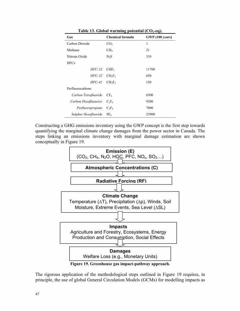
47

Table 13. Global warming potential (CO2-eq). Gas Chemical formula GWP (100 years)

Carbon Dioxide CO2 1

Methane CH4 21

Nitrous Oxide N20 310

HFCs

HFC-23 CHF3 11700

HFC-32 CH2F2 650

HFC-41 CH3F2 150

Perfluorocarbons

Carbon Tetrafluoride CF4 6500

Carbon Hexafluourice C2F6 9200

Perfluoropropane C3F8 7000

Sulphur Hexafluoride SF6 23900

Constructing a GHG emissions inventory using the GWP concept is the first step towards quantifying the marginal climate change damages from the power sector in Canada. The steps linking an emissions inventory with marginal damage estimation are shown conceptually in Figure 19.

Figure 19. Greenhouse gas impact-pathway approach.

The rigorous application of the methodological steps outlined in Figure 19 requires, in principle, the use of global General Circulation Models (GCMs) for modelling impacts as

Emission (E) (CO2, CH4, N2O, HGC, PFC, NOx, SO2…)

Atmospheric Concentrations (C)

Radiative Forcing (RF)

Impacts Agriculture and Forestry, Ecosystems, Energy Production and Consumption, Social Effects

Climate Change Temperature (∆T), Precipitation (∆p), Winds, Soil

Moisture, Extreme Events, Sea Level (∆SL)

Damages Welfare Loss (e.g., Monetary Units)

48

well as multi-sector integrated assessment model (IAM) to quantify the economic outcomes resulting from climate impacts. These steps were outside the scope of this research, and have not been done as part of any other power sector full cost accounting analyses. ExternE used two different external IAM’s, FUND (climate Framework for Uncertainty, Negotiation and Distribution) developed at the Institute for Environmental Studies, Vrije Universiteit, Amsterdam [Tol, 1995, 1996, 1999, 2000], and the Open Framework developed by the Environmental Change Unit, University of Oxford [Downing et al., 1996]. There exists no practical limitation on using these modelling results in for Canadian studies since the geographic location of GHG emissions is irrelevant to assessing the marginal impact of those emissions given the assumption of a well-mixed atmosphere. Canadian emissions are—at the margin—equally responsible for impacts everywhere in the world. The GHG externalities valuation process is similar to the impact-pathways methodology (Figure 19), in that emissions are traced through to their impact endpoints and the damages quantified—with several important caveats [ExternE, 1999b, p.1]: • the geographic location of the emissions source is irrelevant; • the impact complexity makes a disaggregation by impact-pathway impossible; and • the valuation of very long-term effects introduces high uncertainties. Both FUND and the Open Framework model the concentration of the three long-lived anthropogenic GHGs: CO2, CH4 and N2O. The atmospheric GHG concentrations are used to calculate the radiative forcing, which determines average global temperature rise and sea level rise. Both models have been calibrated to IPCC scenario IS92a. The major impacts evaluated by both models are health, agriculture, water supply, sea level rise, ecosystems and biodiversity, and extreme events. FUND uses a non-spatial but inter-temporal dynamic approach that incorporates sensitivity to both the level and rate of climate change. Impacts and damages are aggregated to nine world regions and derived from existing literature. The form of the damage function with respect to temperature increase is developed in considerable detail in the FUND Model. The Open Framework uses a more static approach based on first-order physical impact assessments using a GIS-based tool that links global circulation model (GCMs) results to actual physical impacts, such as loss of agricultural land and wetlands. There is much more emphasis on first-order impacts such as changes in degree-days, areas suitable for agriculture, and hydrologic balance. The Open Framework is disaggregated to the national level. Despite the large differences in model structure between FUND and the Open Framework the marginal damage estimations for CO2 and CH4 and N2O remarkably varied by less than 10 per cent, 20 per cent and 40 per cent [ExternE, 1999] in the base case scenario adopted by ExternE.

49

The similar results between the two models are likely fortuitous; the uncertainty range is very large and important issues such as aspects of socially-contingent damages and ecosystem damages are poorly represented or not included. Human mortality is a major damage component across all impact sectors through the direct effects of extreme temperature, the spread of infectious disease, extreme weather and the socially contingent effects of resource access loss. The mortality valuation methodology is therefore a major determinant of the marginal damages estimation. For any given assumptions on the appropriate mortality valuation method and discount rate (two of many contentious parameters), the calculated marginal damages may well represent a lower bound on actual marginal damages. The proponents of both major models acknowledge, for example, that “the impacts covered by the models used are only a fraction (of unknown size) of all climate change impacts” [Tol and Downing, 2000 p.20]. 4.2.2 GHG Inventory Analysis As a first step towards estimating GHG-related externalities, IISD constructed a GHG inventory for the Canadian power sector with the following features:

• the total emissions by province in kilotonnes (kT) of CO2-eq; • total provincial emissions disaggregate (kT CO2-eq) by fuel type; • emissions intensity by province and fuel type in grams/kWh; and • emissions intensity uncertainty analysis.

Government information sources compile an emissions inventory by province and industrial sector, including the GHG emissions from the electrical generation sector. However, an inventory analysis disaggregated by province and fuel type requires more detailed information on the power generation by fuel type and the quantity of fuel consumed. Table 14 shows 1997 power production by province and fuel type according to National Energy Board statistics [NEB, 1999].15 1997 was chosen as the base year to align as close as possible with the most recent air pollutant emissions data available [Environment Canada, 1998], [CEC, 2002b].

15 For the purposes of this analysis, Heavy Fuel Oil (HFO), Light Fuel Oil (Distillate), and Diesel generation are all treated as “Oil.” Natural gas-based generation via steam cycle, single cycle combustion turbine and combined cycle combustion turbine are all categorized as “Gas.”

50

Table 14. Thermal electric energy production (GWh). Province Coal Oil Gas

Newfoundland 0 1,472 0

P.E.I 21

Nova Scotia 8,036 993

New Brunswick 5,859 4,240

Quebec 889 438

Ontario 23,823 997 9,651

Manitoba 164 21 10

Saskatchewan 11,716 63 875

Alberta 41,685 16 9,067

BC + Territories 0 518 3,922

Canada 91,283 9,230 23,963 Estimating the emissions (in kT CO2-eq) requires the following information:

• the primary energy consumption by province and fuel type in PetaJoules (PJ) [NEB, 1999];

• energy content in GigaJoules (GJ) per tonne of coal and per cubic meter of oil and gas [NCCP, 1999], [Environment Canada, 1999b];

• emissions factors in g/kg for coal, g/l for oil and g/m3 for gas for each of CO2, CH4 and N2O [Environment Canada, 1999b]

• the IPCC standard Global Warming Potential factors for CO2, CH4 and N2O [Environment Canada, 1999b].

The summary emission inventory is shown in Table 15 includes a comparison with the aggregate power sector emissions by province as reported by Environment Canada [EC, 2001b]. The IISD methodology consistently underestimates power sector GHG emissions compared to Environment Canada, with the exception of a one per cent over-estimate in Nova Scotia and, initially, a large over-estimate (105 per cent) in Quebec. Two main factors are responsible for these discrepancies:

1. The Environment Canada category for power sector emissions includes a small amount of combined heat and power production with the effect of biasing total emissions slightly upwards.

2. GHG emissions factors vary widely with the fuel grade, for example the various coal grades: anthracite, lignite, bituminous, etc. The exact composition of the fuel mix in each province was not known and was estimated from secondary sources [NEB, 1999], [Environment Canada, 1999b].

51

A large discrepancy between NEB and Environment Canada data in Quebec could not be readily reconciled, and IISD used the lower estimate for Quebec (shown in Table 15). We believe, therefore, that these emissions (17 per cent below Environment Canada’s estimate) are a consistent under-estimate of actual power sector emissions.

Table 15. Thermal electric GHG emissions (kT CO2-eq).

Province Coal Oil Gas TotalEnvironment

CanadaEstimate

%Difference

Newfoundland 0 1,194 0 1,194 1,210 -1P.E.I 0 25 0 25 39 -36Nova Scotia 7,167 646 0 7,812 7,520 4New Brunswick 4,951 2,502 769 8,221 8,300 -1Quebec 0 361 98 459 459 0Ontario 16,320 762 2,515 19,598 25,800 -24Manitoba 181 20 3 203 233 -13Saskatchewan 13,446 50 463 13,959 15,000 -7Alberta 35,125 14 4,051 39,191 51,300 -24BC + territories 0 341 1,200 1,542 1,627 -5 Canada 77,190 6,294 9,201 92,684 111,000 -17

Table 16 shows the GHG intensity (g/kWh), the total emissions (Table 15) divided by energy production for each province and fuel type (Table 14). Environment Canada reports a five per cent and 40 per cent uncertainty for CO2 and CH4 emissions factors respectively. No uncertainty range is given for N2O. Table 17 shows the one standard deviation uncertainty range for emissions intensity, which is almost exactly five per cent given that power sector GHG emissions as CO2 are about three orders of magnitude greater than CH4 and N2O combined. This uncertainty range is, however, an under-estimate given the lack of knowledge about the exact composition of the fuel mix.

52

Table 16. Thermal electric generation GHG intensity (g/kWh). Province Coal Oil Gas Newfoundland 0 811 0 P.E.I 0 1,186 0 Nova Scotia 892 650 0 New Brunswick 845 590 0 Quebec 0 832 457 Ontario 685 764 261 Manitoba 1,103 942 253 Saskatchewan 1,148 791 529 Alberta 843 870 447 BC + territories 0 659 306 Weighted Avg. 846 682 384

Table 17. GHG intensity: standard deviation (g/kWh).

Province Coal Oil Gas Newfoundland 0.0 40.5 0.0 P.E.I 0.0 59.2 0.0 Nova Scotia 44.3 32.5 0.0 New Brunswick 41.9 29.5 0.0 Quebec 0.0 41.6 22.8 Ontario 33.9 38.2 13.0 Manitoba 54.6 47.0 12.6 Saskatchewan 56.7 39.5 26.3 Alberta 41.8 43.4 22.3 BC + Territories 0.0 32.9 15.3

Weighted Avg. 41.9 34.0 19.1 4.2.3 Climate Change Damages Estimation Monetizing climate change impacts requires an internally consistent valuation strategy for aggregating global damages since all GHG emissions—regardless of their physical location—are equivalent in the sense that they contribute equally to impacts and damages. Conducting research in support of ExternE, Tol and Downing [2000] tackled the global aggregation issue from four different perspectives (after Fankhauser et al. [1997]):

1. from the narrow perspective of a European decision-maker concerned only EU impacts and with EU-level valuations on impacts;

2. (1), plus impacts in other regions of the world with local values;

53

3. (1), plus impacts in other regions with globally averaged values; and 4. (1), plus impacts in other regions with EU values.

Although perspective 1 ignores non EU impacts, it most closely resembles the real-politic of the European decision-maker that the ExternE project is attempting to influence. Perspective 2 values damages at the expressed willingness-to-pay of people outside the EU, which the difficult and potentially objectionable implication that the value of life lost from climate change impacts in, for example Bangladesh is worth less than one lost in the EU. Perspective 3 uses globally averaged damage valuations and Perspective 4 values all impacts regardless of region at EU values. Table 18 lists the marginal costs per tonne of CO2 as calculated using FUND 1.6 for three different social discount rates in year 2000 U.S. dollars. Valuations from the FUND 1.6 model are used in this analysis as this model has been extensively peer-reviewed for use in the ExternE project and use a statistical life valuation methodology consistent with that used in AQVM. For the purposes of this analysis, the third perspective (globally averaged values) is used. Perspective 3 was chosen as the standard central estimate assumption for ExternE work and moreover is the most philosophically consistent with the United Nations Framework Convention on Climate Change (UNFCCC) principle of “common but differentiated responsibilities” among parties (to which Canada is a signatory). [Fankhauser al, 1997].

Table 18. Marginal cost of carbon dioxide emissions (USD/t CO2). Source: Tol and Downing [2000]

Discount Rate

EU Only

Regional Values

World Average

EU Values

0% 0.60 10.61 29.86 123.90 1% 0.46 7.12 20.13 82.55 3% 0.22 3.35 10.09 40.99

The EU-only perspective shows, unsurprisingly, the lowest marginal cost, whereas modelling all global impacts at EU levels (perspective 4) has the highest costs. Table 18 also illustrates the influence of discount rate. Climate change is long-term problem, hence the choice in how future impacts are discounted has critical implications for valuating the marginal costs of emissions today. Tol and Downing [2000] recap the reasons for discounting the future

• Impatience and myopia: consumption today is preferable to consumption tomorrow.

• Economic growth: a dollar today is worth more than in the future because people in the future will be richer.

• Changing relative prices: some impacts, for example on human health, may be valued more in the future.

• Uncertainty: because consumption in the future is not certain, it is worth less than consumption today

54

Of these reasons, only the third argues for a negative discount rate; however the clear recognition that climate change has multi-generational equity implications that should not be minimized leads inevitably to a much lower discount rate than used in conventional cost-benefit analysis (typically 8–12 per cent). The Canadian Analysis and Modelling Group (AMG) argued in their air quality co-benefits study that the appropriate social discount rate for their 20-year period of interest should be two to three per cent, which is consistent with general practice for regulatory analysis in the U.S. [AMG, 2000]. The standardized period of interest for analyzing climate change impacts using IAMs such as FUND is 100 years. The IPCC also uses a standard 100-year period for calculating the equivalent global warming potential of different GHGs, the credits of which are then fungible under the Kyoto Protocol. These considerations argue strongly for low non-negative discounting of future climate change impacts, and therefore, consistent with the central estimates of Tol and Downing [2000], we adopt a one per cent social discount rate, which from Table 18, corresponds to $20.13 USD/t CO2 in year 2000 dollars ($26.36 in 1996 Canadian dollars). Our estimate is in the low range of published values. As part of the IPCC Second Assessment Report, Pearce et al. [1996] surveyed the extant literature finding that the published values for CO2 marginal costs ranged from $5/t to $125/t. De Leo et al. [2001] used a central estimate of 30 Euros/t and a sensitivity range of 0–250 Euros/t. Furthermore on the basis of the precautionary principle, since GHG externality estimations comprise only a fraction (of unknown size) of all climate change impacts, using a marginal cost at the extreme low end of the published range could be construed as particularly imprudent [Krewitt, 2002]. Tol and Downing [2000] also provide estimates of uncertainty based largely on the analysis of Tol [2000]. Similar to the uncertainty methodology used with AQVM, Tol [2000] used Monte Carlo sampling to generate uncertainty ranges based on random sampling of the hypothesized probability distributions of the underlying parameters in the FUND 2.0 model. Tol’s resulting distribution of CO2 marginal cost estimates is approximately log-normal (skewed to the left); however some interpretation caution is advised. First, Monte Carlo analysis captures only parameter uncertainty and not fundamental model uncertainty, and as such represents a lower bound on the true uncertainty. Second, Tol [2000] notes that the probability distributions for the key parameters in FUND are not known and largely based on judgement. For the purposes of this analysis we re-scaled the standard deviation estimates from the FUND 2.0 model [Tol and Downing, 2000] for the World Average Valuation / one per cent discount rate case to the corresponding FUND 1.6 mean marginal CO2 damage estimate.16 The adjusted standard deviation estimate is $18.03 in 1996 Canadian dollars. The global warming externalities for the Canadian thermal power sector are calculated by multiplying the weighted Canadian average GHG intensity (Table 16) by the mean marginal damage estimate, and are shown in Figure 20.

16 Tol and Downing [2000] provide no uncertainty estimates for the FUND 1.6 model. The mortality valuation methodology in FUND 2.0 is inconsistent with that endorsed by Health Canada and Environment Canada as implemented in AQVM, hence FUND 2.0 uncertainty estimates were scaled linearly to the FUND 1.6 mean estimate of marginal CO2 estimates.

55

The uncertainty bounds shown in Figure 20 represent the effect of propagating the uncertainty in GHG intensity (Table 17) with the uncertainty in the marginal cost estimation and assume that we can approximate the probability distribution of both as normal.

0.0223

0.0180

0.0101

$0.000

$0.005

$0.010

$0.015

$0.020

$0.025

$0.030

$0.035

$0.040

COAL GAS OIL

Figure 20. Thermal power global warming externalities in Canada ($/kWh).

4.3 Aggregate Externalities and Uncertainty Analysis The aggregation of air quality and global warming externalities for the thermal power sector in Canada is accomplished by summing the mean air quality externality estimate with the mean global warming externality estimate. The uncertainty bounds shown in Figure 21 are also calculated by propagating the air quality and global warming standard deviation estimates. Similar to the AMG [2000] approach, we assume that the mean of

the 17th and 83rd percentile bounds on air quality externalities estimated with AQVM approximates the standard deviation. This uncertainty estimate is then combined with that of global warming externalities to produce an aggregate standard deviation estimate.

56

Figure 21. Thermal power air quality and global warming externalities in Canada ($/kWh).

$0.0218

$0.0394

$0.0102

$0.000

$0.010

$0.020

$0.030

$0.040

$0.050

$0.060

$0.070

COAL GAS OIL

For comparison, Table 15 shows the central estimates (in 1996 Canadian dollars) for the same three fuel cycles from the ExternE country study in the United Kingdom [ExternE, 1998]. Several factors explain the higher U.K. estimates. First, the U.K. study evaluated a larger set of damage endpoints particularly those related to upstream impacts in the various fuel cycles such as occupational health damages. Second, converting the willingness-to-pay to avoid health related damages is more complicated than the simple currency adjustment used to present the values in Table 19. Nonetheless the broad agreement between these independent studies provides confidence that the range presented for Canadian thermal power externalities is reasonable.

Table 19. U.K. ExternE results ($ CDN/kWh 1996). Coal Oil Gas Canada U.K. Canada U.K. Canada U.K. Public Health 0.017 0.035 0.004 0.03 0.0001 0.005 Global Warming 0.022 0.043 0.018 0.031 0.01 0.019 Other n/a 0.004 n/a 0.002 n/a 0 Sub-total 0.039 0.082 0.022 0.063 0.01 0.025

57

4.4 Sources of Uncertainty and Biases The uncertainty bounds presented in this study reflect only the parameter uncertainty of the costed pathways and do not address fundamental uncertainty and systematic bias. For completeness we provide a list of fundamental uncertainties and known biases in our analysis all of which we believe biases our analysis downward with respect to the total externality burden from the Canadian thermal power sector in 2003. The central estimates for power sector externalities presented in this paper are therefore believed to be a conservative under-estimate. Fundamental Uncertainties (damage functions known to exist but data not available)

• Carbon Monoxide causing cardiac hospital admissions (bias downward) • Acid Deposition impacting fishing yields (bias downward) • Air toxins and risks of cancers, neurological disorders17 (bias downward) • Ozone damages on forests and agricultural crops18 (bias downward)

Fundamental Uncertainties (damage functions unknown but believed to exist)

• NOx emissions impacts on agriculture and ecosystems (bias downward) • Air toxics impacts on terrestrial wildlife (bias downward) • Acid deposition impacts on ecosystems (bias downward)

Systematic Analytical Biases

• Power production statistics are not perfectly aligned with 1995–1998 air emissions data; (bias downward with respect to total externalities, unknown with respect to unit externalities).19

• 17 per cent systematic under-estimate of GHG emissions (bias downward) • No air quality externalities in Western Canada (bias downward) • No air quality externalities from Eastern Canadian

sources with U.S. receptors (bias downward) • Atmospheric transport mechanisms (bias unknown) • No upstream source-receptor model for gas (bias downward) • GHG costs a subset of unknown size of all impacts (bias downward) • Mortality valuation methodology (bias unknown, possibly upward)

17 The Commission for Environmental Cooperation (CEC, 2000) has identified mercury emissions from coal-fired power generation as a priority concern. http://www.cec.org/programs_projects/pollutants_health/smoc/pdfs/Hgnarap.pdf The Canadian Council of Ministers of the Environment (CCME) is developing Canada-Wide Standards for mercury emissions, the first stage of which is a monitoring and reporting program to guide the collection, verification and reporting of mercury emissions data from the electric power generation sector prior to 2005. http://www.ccme.ca/initiatives/standards.html?category_id=53 18 Ozone damage functions for agricultural are available in AQVM, however they are suspected to systematically under-estimate damages and are currently in review [O’Gorman-Stinson, 2002] They were therefore not included in this analysis 19 The 1998 SOx emissions data in Ontario may not fully reflect the recent measures taken by OPG to reduce SOx emissions such as the use of low-sulphur coal and the installation of SO2 scrubbers on 2 of 8 combustion units at Nanticoke resulting in an upward bias of unit externality costs. However, our estimate of the coal-fired GHG emission intensity for Ontario (685 g/kWh) is considerably lower than actually reported by OPG in their Towards Sustainable Development: 2001 Progress Report (~900 g/kWh) suggesting a downward bias. http://www.opg.com/envComm/SED2001Report.pdf

58

5 Policy Implications

5.1 Kyoto Compliance Canadian thermal power sector externalities can not be known exactly, however they are clearly non-zero. The fundamental policy implication is that if Canadian thermal power producers had to internalize externalities via taxation or by the purchase of tradable permits, power sector emissions would decrease because it would be economic to do so. Reducing emissions from coal-fired power generation should be a particularly important policy objective. The central estimate of coal externalities from this study ($0.0394/kWh) is about 50 per cent higher than the marginal cost of production for coal.20 Neglecting global warming damages, just the central estimate of the public health externalities ($0.0171/kWh) is 65 per cent of the marginal production cost. Electricity prices for power generated by natural gas are significantly less distorted by the failure to internalize externalities. Our central estimate for gas externalities ($0.0102/kWh) is approximately 20 per cent of the estimated marginal production cost. Public health externalities for gas are negligible—about 0.2 per cent of the marginal production cost.21 Canada’s recent Kyoto ratification provides new impetus for re-visiting the mix of generation technologies within the Canadian power sector. The Kyoto Protocol allows countries to reduce their own emissions or buy lower-cost emission reduction credits internationally. The Government of Canada’s Climate Change Action Plan [Government of Canada, 2002], Canada’s nascent strategy for Kyoto compliance, treats the thermal power sector within the Large Industrial Emitters category and is proposing that individual firms initially receive free GHG emissions permits equivalent to 85 per cent of their baseline emissions. The supply of permits to individual firms would then grow or shrink over time based on the firm’s emissions intensity factor, reflecting the firm’s relative energy efficiency. The basic rationale for the emissions intensity approach is that it provides a continued incentive to reduce emissions but does not place an absolute cap on any firm’s emissions. Reconciling the emissions intensity approach with the absolute caps on national emissions and with the government’s commitment to cap the cost to large emitters of international emissions reduction credits at $15/tonne creates a potential liability for the federal government. If the GHG permit allocation strategy based on emissions intensity fails to produce the required absolute emissions reductions required to meet the national cap, the federal government will have to purchase emissions reduction credits on the international market (which may conceivably cost more than $15/tonne). The Climate Change Action Plan provides illustrative examples of the expected price signal seen by different economic sectors under the current federal plan for Kyoto compliance.22 Coal-fired power production will see a price increment of 1.94% of the wholesale cost of production, “potentially raising competitiveness issues” [Government

20 $0.026/kWh source: The Nanticoke Conversion Study, Diener Consulting Inc. 2001, p.19. 21 $0.05/kWh Ibid., p.15. 22 The scenarios shown assume 85 per cent free permit allocation and $10/tonne unit carbon price

59

of Canada, 2002, p.32]. A fundamental concern is that the thrust of the Canadian Kyoto compliance strategy will be to make the price signal seen by large emitters (including coal-fired power generators), small enough so that appropriate levels of emission reductions are not realized. The ultimate implication is that the federal government bears a significant risk that it must purchase emissions reduction credits on international markets to achieve the national target and thus forego the large domestic benefits of reduced public health and global warming externalities if domestic emitters had instead reduced emissions.

Internalizing Externalities: Effects on Power Sector Investment Decision-Making The case of Nanticoke, the largest single thermal power plant in Canada, provides an interesting illustrative example of the effect of externalities on investment decision-making. Nanticoke is a 3920 MW coal-fired power plant located on north shore of Lake Erie, directly south of Hamilton. Ontario Power Generation, Nanticoke’s owner-operator, has been heavily criticized in recent years for continuing to operate Nanticoke on coal, primarily because Nanticoke is both the single largest CO2 emissions source and the single largest source of all air pollutants (by total mass) in Canada, according to statistics compiled by the National Pollutant Release Inventory [OCAA, 2002]. The cost of converting Nanticoke to natural gas has been studied by a consortium of consulting engineers sponsored by the Ontario Clean Air Alliance. We illustrate the effects of introducing public health and global warming externalities on the decision to do nothing, convert Nanticoke to natural gas, or displace the energy equivalent to Nanticoke’s annual production by a combination of demand side management (DSM) and renewable energy. The baseline assumptions for the annual cost comparison in the table below are that:

• The capital cost of natural gas conversion is $800 000/MW (2001) and is

annualized at eight per cent over 20 years.23 • Nanticoke’s annual production (21124 GWh) can be met by either natural gas

$0.05 kWh (operating cost)24 or by a combination of DSM and wind at $0.058/kWh in capital costs + $0.005/kWh operating costs.25

• Conversion to natural gas reduces GHG emissions by 61 per cent and generates carbon credits at $10/tonne. Displacement by DSM + renewable energy generates carbon credits equal to 100 per cent of Nanticoke’s GHG emissions.

• The public health and global warming externalities are valued at the central estimates given in this study.

• The wholesale value of energy is equivalent in all cases and not shown.

23 The Nanticoke Conversion Study, Diener Consulting Inc. 2001, p.13. 24 Ibid., p.15. In July 2003, the NYMEX futures price for natural gas delivered in January 2005 was $7.35 CAD/mcf, (trending lower), an increase of about 17 per cent over the base case estimate in the Diener et al. (2001) study and suggests that the operating costs for natural gas conversion presented in Table 20 may be under-estimated. 25 Based on the unit cost for a large-scale wind power project in Quebec in 1999 cited in Low-impact renewable energy policy in Canada: Strengths, Gaps and a Path Forward, Pembina Institute for Appropriate Development, 2003. Pembina also notes in this study that unit wind power costs continue to drop. Wind power is an intermittent resource and not strictly comparable to base-loaded coal power, however a large, geographically dispersed wind resource has the long-term effect of displacing all of the generation modes in the mix of grid power and not strictly coal-fired generation.

60

Table 20. Full cost analysis of Nanticoke conversion in millions of dollars annually. Benefits Costs Externalities Total Annual Cost

Carbon Sales Capital Operating

PublicHealth

Global Warming

incl. Externalities

w/o Externalities

Do nothing 0.0 0.0 -575.9 -359.1 -464.7 -1,399.7 -575.9 Natural gas conversion 123.6 -316.9 -1,056.2 -2.11 -211.2 -1,462.8 -1,249.5 DSM and renewables 202.6 -1,225.2 -105.6 0.0 0.0 -1,128.2 -1,128.2

The influence of externalities on the least cost option is clear in this illustrative example. Conversion to natural gas is only slightly more costly than “do nothing,” and the economic argument is much weaker, particularly since the co-benefits of natural gas conversion are increased compliance with existing air quality regulatory requirements.26 A combination of DSM and renewable energy is the least-cost option by a significant margin. Furthermore this analysis does not account for the risk of natural gas price volatility. Table 20 shows the conversion costs for an existing power plant whose ongoing capital costs are assumed to be zero. Such an analysis would typically be undertaken when the existing plant was nearing the end of its design life, and simply maintaining the plant required significant capital expenditure, which would have the effect of favouring natural gas conversion or DSM and renewable energy alternatives. In the case of an investment decision for a completely new power plant, the argument tilts further in favour of natural gas or DSM and renewable energy when externalities are included.

26 Canada is already a signatory to

• the Ozone Annex to the 1991 Canada-United States Air Quality Agreement that requires that total nitrogen oxide emissions in southern Ontario be capped.

• Canada is also committed to : o The Canada-Wide Acid Rain Strategy for post 2000, which mandates to SO2 emissions reductions, and , o The Canada-Ontario Agreement Respecting the Great Lakes Basin Ecosystem, a management framework for

reducing toxic pollutants in the Great Lakes.

61

6 Conclusions The explicit calculation of environmental externalities can and should inform energy sector policy-making, however this is not routinely the case in Canada or elsewhere. The Kyoto Protocol is an attempt however to internalize, if not the full costs, at least the risk of serious anthropogenic alternation to the global climate system. Canada’s ratification of the Kyoto Protocol also provides the policy context for re-examining the structure of the energy sector from an externalities perspective. Integrating externalities into the investment decision process is particularly important for the power sector, given the large environmental burdens of conventional thermal power and the slow turn-over of capital stock. This study is the first in Canada to use regional scale source-receptor modelling to quantify the air quality and global warming externalities associated with thermal power generation. Our analysis indicates that the air quality and global warming externalities associated with coal-fired electricity production are approximately equal, whereas for oil and gas-fired power, air quality externalities are one and two orders of magnitude respectively less than global warming damages. Both the relative and absolute magnitudes of the externalities coasted in this study compare well to other studies. We believe, however, that because many impact-pathways remain uncosted our externality estimates are conservative A particular important immediate implication of this study concerns Canada’s Kyoto implementation strategy. The Kyoto Protocol allows countries to reduce their own emissions or buy lower cost emission reduction credits internationally. Full cost estimates of thermal power production, such as those reported here can be used to guide the Kyoto compliance strategy, particularly with respect to the magnitude of domestic benefits foregone if international emissions trading is used preferentially to domestic emissions reduction. Coal-fired generation should be particularly closely scrutinized as the magnitude of the externalities burden is in the same range as the marginal production cost.

62

References Abbey et al. [1995a]. Abbey, D.E., B.D. Ostro, F. Petersen, and R.J. Bruchette. 1995a. Chronic Respiratory Symptoms Associated with Estimated Long-term Ambient Concentration of Fine Particulates <2.5 Aerodynamic Diameter (PM2.5) and Other Air Pollutants. Journal of Exposure Analysis and Environmental Epidemiology 5:137-150. Abbey et al. [1995b]. Abbey, D.E., M.D. Lebowitz, P.K. Mills, F.F. Petersen, W.L. Beeson, and R.J. Burchette. 1995b. Long-term Ambient Concentrations of Particulates and Oxidants and Development of Chronic Disease in a Cohort of Nonsmoking California Residents. Inhalation Toxicology 7:19-34. ABDOE [1996]. Full Fuel Cycle Emissions Analysis of Existing and Future Electric Power Generation Options in Alberta, Canada. Alberta Department of Energy, 1996. AMG [2000]. Analysis and Modelling Group. The Environmental and Health Co-benefits of Actions to Mitigate Climate Change, Report of the Environmental and Health Impacts (EHI) Subgroup to the Analysis and Modelling Group, National Climate Change Process. November 2000. Ayres and Kneese [1969]. Ayres, Robert U. and Allen V. Kneese. Production, Consumption and Externalities, American Economic Review, LIX, June 82-97. Bernow and Marron [1990]. Bernow, S. S. and Marron, D. B. 1990. Valuation of Environmental Externalities for Energy Planning and Operations, Tellus Institute, Boston. Burnett et al. [1997]. Burnett, R.T., J.R. Brook, W,.T. Yung, R.E. Dales, and D. Krewski. 1997. Association between Ozone and Hospitalization for Respiratory Diseases in 16 Canadian Cities. Environmental Research 72:24-31. Burnett et al. [1995]. Burnett, R.T., R. Dales, D.Krewski, R. Vincent, T. Dann, and J.R. Brook. 1995. Associations between Ambient Particulate Sulphate and Admissions to Ontario Hospitals for Cardiac and Respiratory Diseases. American Journal of Epidemiology 142(1):15-22. CIHI [1994]. Canadian Institute for Health Information. 1994. Resource Intensity Weights: Summary of Methodology 1994/95. Don Mills, Ontario. [CNN, 2002]. UN: Environmental messes cost billions, CNN, October 31, 2002. http://www.evworld.com/databases/shownews.cfm?pageid=news311002-07 [CEC, 2001]. Commission for Environmental Cooperation, 2001. The North American Mosaic: A State of the Environment Report, Commission for Environmental Cooperation: Montreal.

63

CEC [2002a]. Comission for Environmental Cooperation, 2002. Environmental Challenges and Opportunities of the Evolving North American Electricity Market: Secretariat Report to Council under Article 13 of the North American Agreement on Environmental Cooperation, Comission for Environmental Cooperation: Montreal. CEC [2002b]. Comission for Environmental Cooperation, 2002. Estimating Future Air Pollution from New Electric Power Generation. Working Paper, Comission for Environmental Cooperation: Montreal DeLeo et al. [2001]. DeLeo, G. A., Rizzi, L., Caizzi, A and Gatto, M. The Economic benefits of the Kyoto Protocol. Nature V413 pp478-479. Dockery et al. [1996]. Dockery, D.W., J. Cunningham, A.I. Damokosh, L.M. Neas, J.D. Spengler, P.Koutrakis, J.H. Ware, M. Raizenne, and F.E. Speitzer. 1996. Health Effects of Acid Aerosols on North American Children: Respiratory Symptoms. Environmental Health Perspectives 104:500-505. Diener et al. [2001]. The Nanticoke Conversion Study. Diener Consulting Inc. April 2001. Downing et al. [1996]. Downing, T. E., Eyre, N., Greener, R, Blackwell, D. 1996. Projected costs of climate change for two reference scenarios and fossil fuel cycles. Environmental Change Unit, Oxford. [Duc et al., 2000]. Duc, H., I. Shannon, M. Azzi, 2000. Spatial distribution characteristics of some air pollutants in Sydney. Mathematics and Computers in Simulation 54 pp.1-21. EC [1996]. European Commission/OECD/International Energy Agency workshop, 1996. Environment Canada [1997a]. Environment Canada, Canadian Acid Rain Assessment, Volume 2, Atmospheric Science Assessment Report, Supply and Services Canada, 302 pp., 1997. Environment Canada [1997b]. Atmospheric Science Expert Panel Report, Joint Industry/Government Study, Sulphur in Gasoline and Diesel fuels, Study Secretariat, Environment Canada, August 14, 1997. Environment Canada [1998]. Environment Canada, 1995 Criteria Air Contaminant Emissions for Canada, 1998.

Environment Canada [1999a]. Environment Canada, Canada’s Greenhouse Gas Inventory:1997 Emissions and Removals with Trends, 1999. Environment Canada [1999b]. Environment Canada Air Quality Valuation Model, Version 3.0

64

Environment Canada [2001a]. Precursor Contributions to Ambient Fine Particulate Matter in Canada, 2001. Environment Canada [2001b]. Information on Greenhouse Gas sources and sinks. http://www.ec.gc.ca/pdb/ghg/ (last accessed 2003.01.20) Environment Canada [2002a]. Acid Deposition and Oxidants, Air Quality Research Branch, URL: www.msc.ec.gc.ca/aqrb/issuesado_e.cfm [last accessed 2003.01.09] Environment Canada [2002b]. Canada Country Study: Climate Impacts and Adaptation Policy Summary http://www.ec.gc.ca/climate/ccs/policysummary_e.htm (last accessed 2002.10.15) EPA [1996]. US EPA, Full Cost Accounting for Decision-Making at Ontario Hydro: A Case Study. ExternE [1998]. European Commission. ExternE: Externalities of Energy Vols 1-6 (EC, Brussels, 1998) (http://externe.jrc.es/index.html) ExternE [1999a]. European Commission. ExternE: Externalities of Energy Vol. 7 Methodology 1998 Update (EC, Brussels, 1999) (http://externe.jrc.es/index.html) ExternE [1999b]. European Commission. ExternE: Externalities of Energy Vol. 8 Global Warming (EC, Brussels, 1999) (http://externe.jrc.es/index.html) Federov [1989]. Federvo, V. V., 1989. Kriging and other estimators of spatial field characteristics (with special reference to environmental studies). Atmos. Environ., 23, 175-184. Fung et al. [1991]. Fung, S. C., P. K. Misra, R. Bloxam, and S. Wong. A numerical experiment on the relative importance of H202 and 03 in aqueous conversion of SO2 to SO2-

4 Atmos. Environ., 23, 175-184, 1989. Government of Canada [2002]. Climate Change Plan for Canada. available at http://www.climatechange.gc.ca Hohymeyer [1988]. Hohymeyer, O. The Social Costs of Energy Consumption. Springer-Verlag, Berlin. IPCC [2001]. Inter-governmental Panel on Climate Change, Technical Summary, Climate Change 2001: Impacts, Adaptation and Vulnerability. 2001 Jacques-Whitford [2000]. Jacques Whitford Environmental Limited, Estimating Changes in Ambient Air Quality Due to Changes in Criteria Air Contaminant Emissions Associated with Measures to Reduce Greenhouse Gas Emissions. 2000.

65

Krewitt [2002]. Krewitt, W. External costs of energy – do the answers match the questions? Looking back at 10 years of ExternE. Energy Policy 30, 839-848, 2002. Krupnick and Cropper [1989]. Krupnick, A.J., and M.L. Cropper. 1989 Valuing Chronic Morbidity Damages: Medical Costs, Labor Market Effects, and Individual Valuations. Final Report to U.S. EPA, Office of Policy Analysis. Krupnick and Cropper [1992]. Krupnick, A.J., and M.L. Cropper. 1992. The Effect of Information on Health Risk Valuations. Journal of Risk and Uncertainty 5:29-48. Krupnick and Kopp [1988]. Krupnick, A.J., and R. Kopp. 1988. The Health and Agricultural Benefits from Reductions in Ambient Ozone in the United States. Resources for the Future, Washington, D.C. Discussion Paper QE88-10. Krupnick et al. [1990]. Krupnick, A.J., W. Harrington, and B.Ostro. 1990. Ambient Ozone and Acute Health Effects: Evidence from Daily Data. Journal of Environmental Economics and Management 18(1):1-18. Loeman et al. [1979]. Loehman, E.T., S.V. Berg, A.A. Arroyo, R.A. Hedinger, J.M. Schwarts, M.E. Shaw, R.W. Fahien, V.H. De, R.P. Fishe, D.E. Rio, W.F. Rossley, and A.E.S. Green. 1979. Distributional Analysis of Regional Benefits and Cost of Air Quality Control. Journal of Environmental Economics and Management 6:222-243. Misra et al. [1989]. Misra, P. K., R. Bloxam, C. Fung, and S. Wong, Non-linear response of wet deposition to emissions reduction: a model study, Atmos. Environ, 23 671-687, 1989. Moran [2001]. Moran, M. Air Quality Research Branch, Meteorological Service of Canada, Environment Canada (personal communication), 2001. Munich RE [2002]. Topics: Natural Catastrophes, January-September 2002. Munich, Munchener Ruckversicherungs-Gesellschaft. NEB [1999]. Canadian Energy Supply to 2025. National Energy Board, Ottawa. NCCP [1999]. Analysis and Modelling Group/Natural Resources Canada. Canada’s Energy Outlook: An Update. 1999. NRCan [2001]. Natural Resources Canada, Energy Efficiency Trends in Canada 1990 to 1999: An Update. 1999 Ostro et al. [1989]. Ostro, B.D., and S. Rothschild. 1989. Air Pollution and Acute Respiratory Morbidity: An Observational Study of Multiple Pollutants. Environmental Research 50:238-247.

66

Ostro [1990]. Ostro, B.D. 1990. Associations between Morbidity and Alternative Measures of Particulate Matter. Risk Analysis 10:421-427. Ostro et al. [1991]. Ostro, B.D., M.J. Lipsett, M.B. Wiener, and J.C. Selner. 1991. Asthmatic Responses to Airborne Acid Aerosols. American Journal of Public Health 81:694-702. Ostro et al. [1993]. Ostro, B.D., M.J. Lipsett, J.K. Mann, A. Krupnick, and W. Harrington. 1993. Air Pollution and Respiratory Morbidity among Adults in Southern California. American Journal of Epidemiology 137(7): 691-700. Padro et al. [1991]. Padro, J. G., G. Den Hartog and H. H. Neumann. An investigation of the ADOM dry deposisiton module using summertime O3 measurements above a deciduous forest. Atmos. Environ., 25, 1689-1704, 1991. Pearce et al. [1992]. Pearce, D. W., Bann, C. and Georgiou, S. P., 1992. The Social Costs of Fuel Cycles. HMSO. Pearce [2001]. Pearce, D. W. Energy Policy and Externalities: An Overview. Externalities and Energy Policy: The Life Cycle Analysis Approach. Workshop Proceedingsof the Nuclear Energy Agency/Organisation for Economic Co-operation and Development. Paris, France 15-16 November, 2001. Pembina [2003]. Low-impact Renewable Energy Policy in Canada: Strenths, Gaps and a Path Forward. Pembina Institute for Appropriate Development. 2003 Pigou [1932]. Pigou, A. C. The Economics of Welfare. London. Pope et al. [1995]. Pope, C.A., III, M.J. Thun, M.M. Namboodiri, D.W. Dockery, J.S. Evans, F.E. Speizer, and C.W. Heath, Jr. 1995. Particulate Air Pollution as a Predictor of Mortality in a Prospective Study of U.S. Adults. American Journal of Respiratory and Critical Care Medicine 151:669-674 Rothman et al. [1997]. Rothman, D. S., Demeritt, D., Chiotti, Q., and Burton, I. Costing Climate Change: The Economics of Adpatations and Residual Impacts for Canada in Volume VIII of the Canada Country Study: Climate Impacts and Adaptation, Environment Canada, Hull. Rowe and Chestnut [1986]. Rowe, R.D., and L.G. Chestnut. 1986 Oxidants and Asthmatics in Los Angeles: A Benefits Analysis. Prepared by Energy and Resource Consultants, Inc. Report to the U.S. Environmental Protection Agency, Office of Policy Analysis, Washington, D.C., March. EPA 230-09-86-018. Rowe et al. [1996]. Rowe, R.D., L.G. Chestnut, D.C. Peterson, and C. Miller. 1986. The Benefits of Air Pollution Control in California. (Two volumes). Prepared for California

67

Air Resources Board by Energy and Resource Consultants, Inc., Boulder, Colorado. Contract No. A2-118-32. Schwartz et al. [1996]. Schwartz, J., D.W. Dockery, and L.M. Neas. 1996. Is Daily Mortality Associated Specifically with Fine Particles? Journal of the Air & Waste Management Association 46:927-939 Spadaro and Rabl [2002]. Spadaro, J. V and Rabl, A. 2002. Air pollution damage estimates: the cost per kilogram of pollutant. Int. J. of Risk Assessment and Management 3(1):75-96. Stieb et al. [1995]. Stieb, D.M., R.C., Beveridge, J.R. Brook, R.T. Burnett, A.H. Anis, and R.E. Dales. 1995. Measuring Health Effects, Health Costs and Quality of Life Impacts Using Enhanced Administrative Data: Design and Preliminary Results. Particulate Matter: Health and Regulatory Issues. VIP-49: 131-142. Stock et al. [1988]. Stock, H, B.M. Gehan, P.A. Buffler, C.F. Constant, B.P. His, and M.T. Morandi. 1988. The Houston Area Asthma Study: a Reanalysis. Paper presented at the Annual Meeting of the Air Pollution Control Association, Dallas, Texas, June 19-24. Tolley et al. [1986]. Tolley, G.S., L. Babcock, M. Berger, A. Bilotti, G. Blomquist, R. Fabian, G. Fishelson, C. Kahn, A. Kelly, D. Kenkel, R. Kumm, T. Miller, R. Ohsfeldt, S. Rosen, W. Webb, W. Wilson, and M. Zelder. 1986a. Valuation of Reductions in Human Health Symptoms and Risk. Prepared at the University of Chicago. Final Report for the U.S. EPA, Grant #CR-811053-01-0. January. Tol [1995]. Tol, R., 1995. The Damage Costs of Climate Change: Towards More Comprehensive Calculations. Environmental and Resource Economics, 5, 353-374. Tol [1996]. Tol, R., 1996. The damage costs of climate change: Towards a dynamic representation. Ecological Economics 19, 67-90. Tol [1999]. Tol, R., 1999. New estimates of the damage costs of climate change, Part I: benchmark estimates. D99/02, Institute of Environmental Studies, Vrije Universiteit, Amsterdam. Tol and Downing [2000]. Tol, R. and Downing, T. E., 2000. The marginal costs of climate changing emissions. D-00/08, Institute for Environmental Studies, Vrije Universiteit, Amsterdam. Tolley et al. [1986]. Tolley, G.A., A. Randall, G. Blomquist, R. Fabian, G. Fishelson, A. Frankel, J. Hoehn, R. Krumm, E. Mensah, and T. Smith. 1986b. Establishing and Valuing the Effects of Improved Visibility in Eastern United States. Prepared for the U.S. Environmental Protection Agency, Washington, D.C.

68

Venkatram et al. [1988] Venkatram, A., P. K. Karamchandani and P. K. Misra, Testing a comprehensive acid deposition model. Atmos. Environ. 22, 737-747, 1988. Viscusi et al. [1991]. Viscusi, W.K., W.A. Magat, and J. Huber. 1991. Pricing Environmental Health Risks: Survey Assessments of Risk-Risk and Risk-Dollar Trade-offs for Chronic Bronchitis. Journal of Environmental Economics and Management 21(1):32-51. Whittemore et al. [1980]. Whittemore, A., and Whittemore, A., and E. Korn. 1980. Asthma Whittemore, A., and E. Korn. 1980. Journal of Public Health.