1

The Fourier Transform

Jean Baptiste Joseph Fourier

1768-1830

2

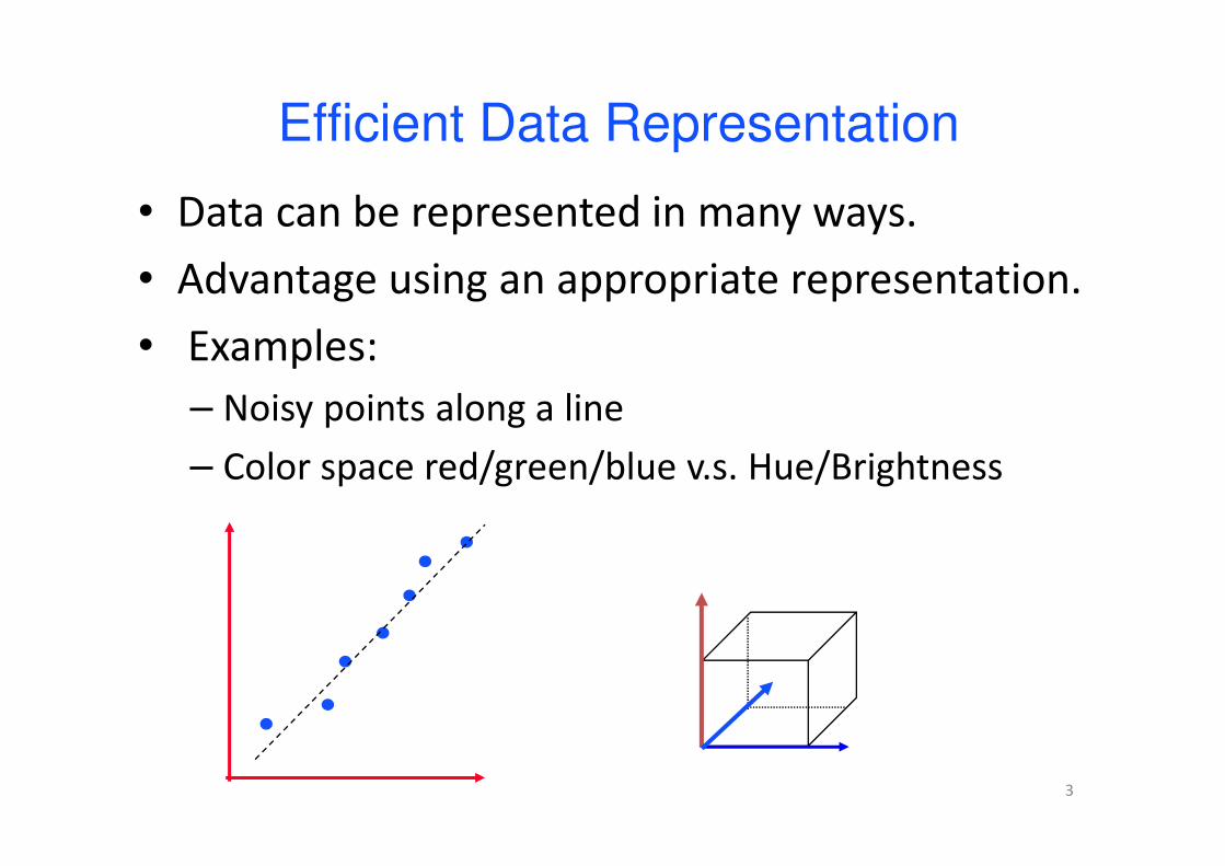
Efficient Data Representation

• Data can be represented in many ways.

• Advantage using an appropriate representation.

• Examples:

– Noisy points along a line

– Color space red/green/blue v.s. Hue/Brightness

3

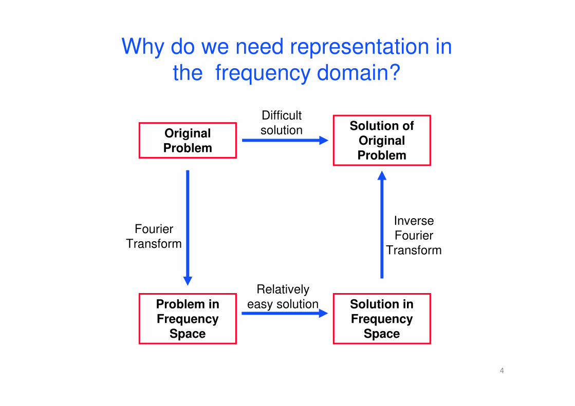
Relatively

easy solution Solution in

Frequency Space

Problem in

Frequency Space

Original Problem

Solution of Original

Problem

Difficult

solution

Fourier

Transform

Inverse

Fourier

Transform

Why do we need representation in the frequency domain?

4

5

How can we enhance such an image?

6

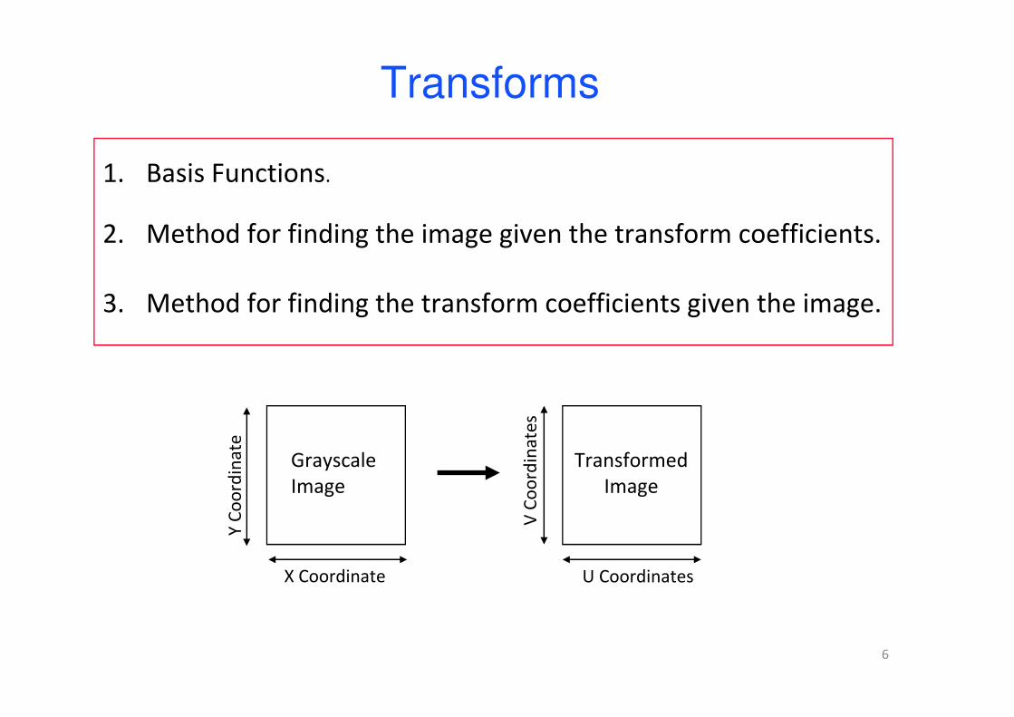
Transforms

1. Basis Functions.

2. Method for finding the image given the transform coefficients.

3. Method for finding the transform coefficients given the image.

U Coordinates

V C

oo

rdin

ate

s

X Coordinate

Y C

oo

rdin

ate

Grayscale

Image

Transformed

Image

7

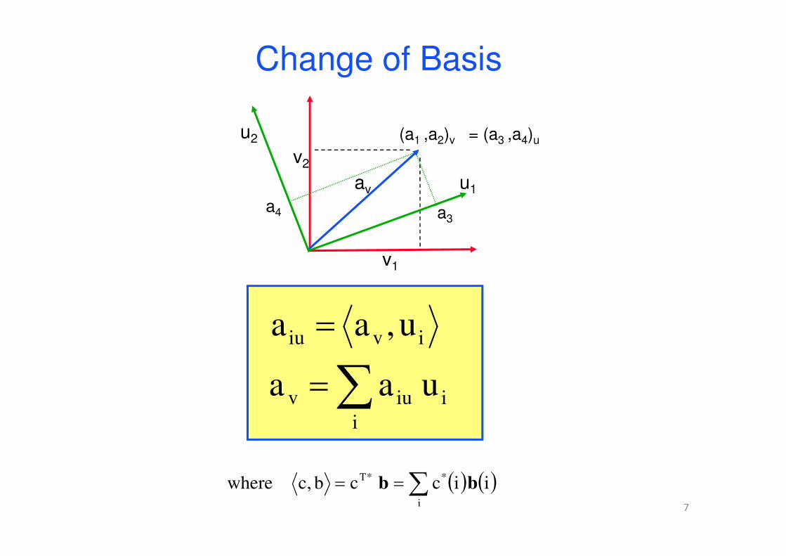
Change of Basis

iviu u,aa =

v2

v1

av

u2

u1

i

i

iuv uaa ∑=

( ) ( )iiccb,cwherei

**Tbb ∑==

(a1 ,a2)v

a3a4

= (a3 ,a4)u

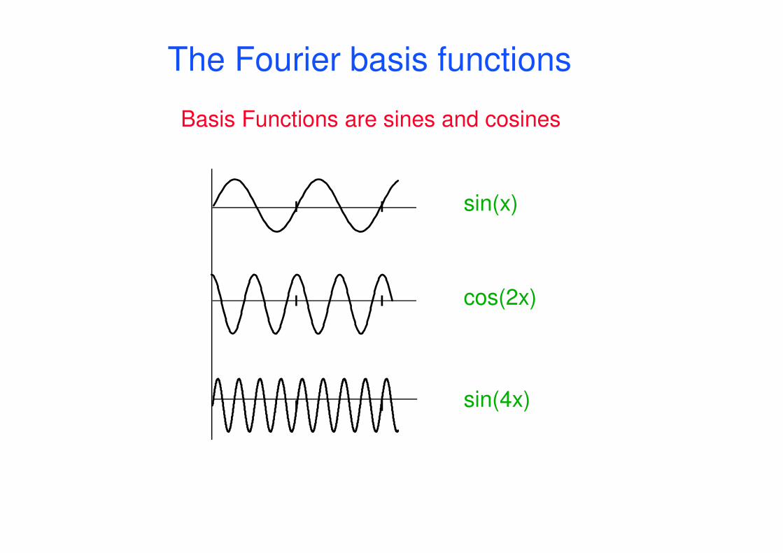
The Fourier basis functions

Basis Functions are sines and cosines

sin(x)

cos(2x)

sin(4x)

9

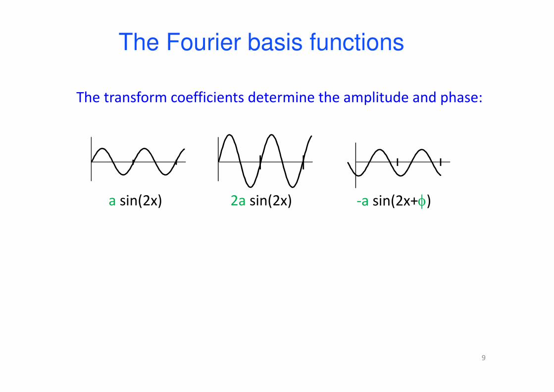
The Fourier basis functions

The transform coefficients determine the amplitude and phase:

a sin(2x) 2a sin(2x) -a sin(2x+φ)

10

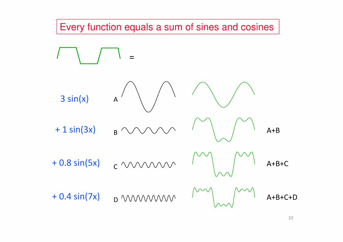
Every function equals a sum of sines and cosines

3 sin(x)

+ 1 sin(3x)

+ 0.8 sin(5x)

+ 0.4 sin(7x)

=

A

B

C

D

A+B

A+B+C

A+B+C+D

11

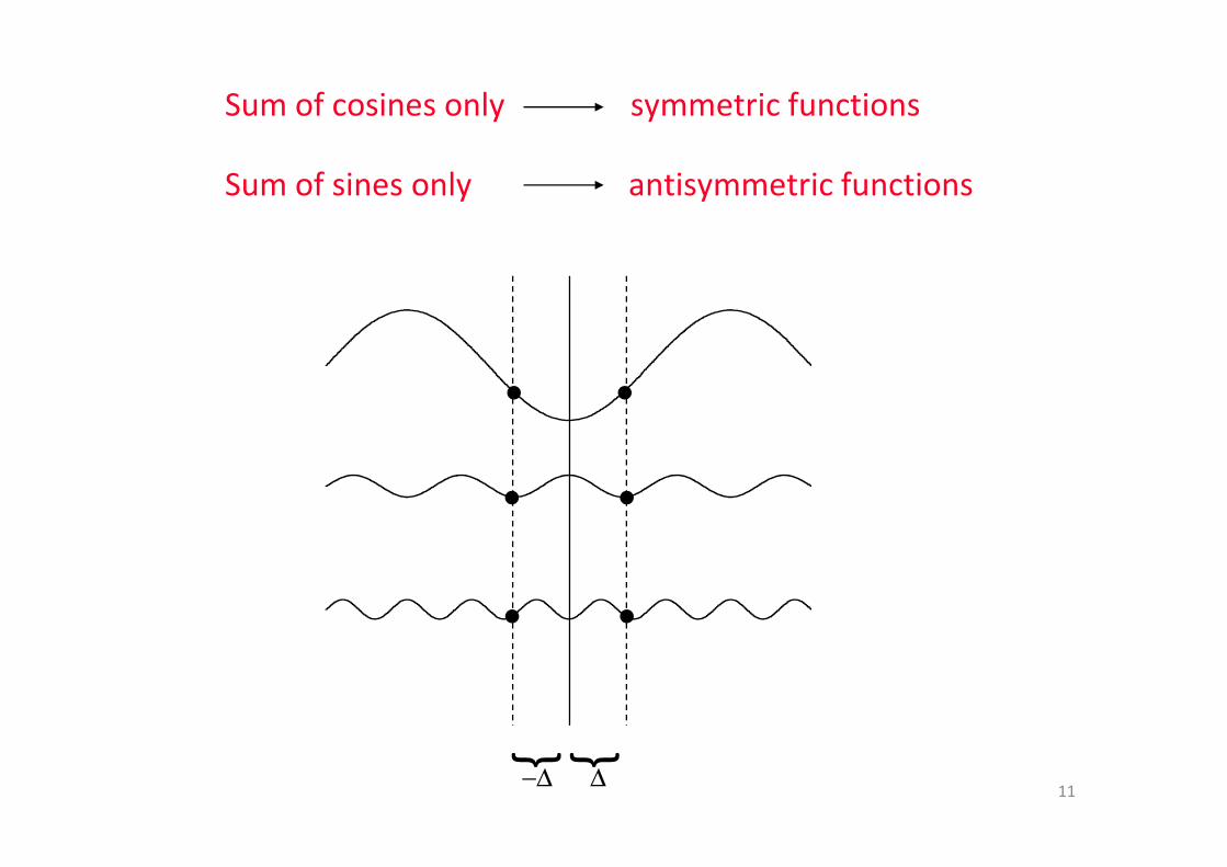
Sum of cosines only symmetric functions

Sum of sines only antisymmetric functions

{ {

∆−∆

12

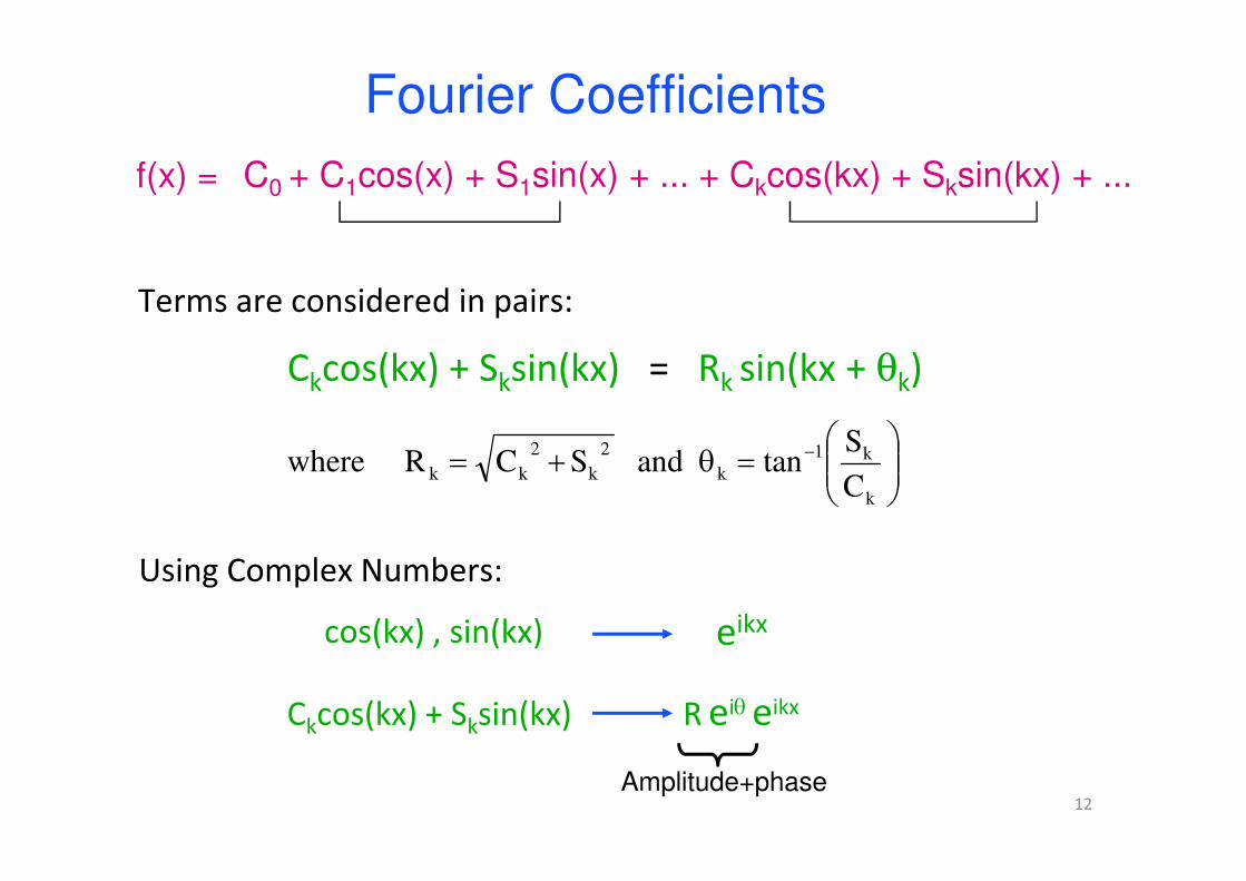
Fourier Coefficients

C0 + C1cos(x) + S1sin(x) + ... + Ckcos(kx) + Sksin(kx) + ... f(x) =

Using Complex Numbers:

Ckcos(kx) + Sksin(kx) = Rk sin(kx + θk)

Terms are considered in pairs:

=θ+= −

k

k1

k

2

k

2

kkC

StanandSCRwhere

cos(kx) , sin(kx) eikx

Ckcos(kx) + Sksin(kx) R eiθeikx

Amplitude+phase

13

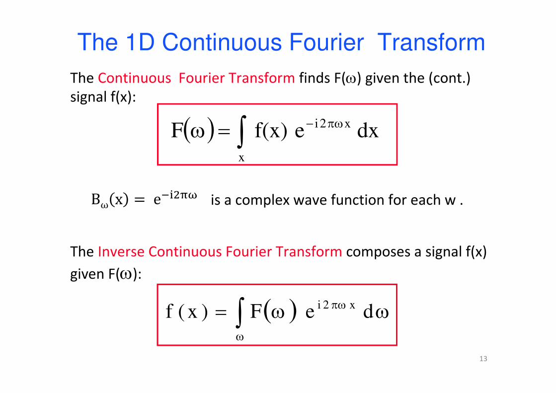
The Inverse Continuous Fourier Transform composes a signal f(x)

given F(ω):

( ) ωω= ∫ω

πω deF)x(f x2i

The Continuous Fourier Transform finds F(ω) given the (cont.)

signal f(x):

( ) dxef(x)Fx

x2i∫ πω−=ω

The 1D Continuous Fourier Transform

is a complex wave function for each w .Bω x = e���

14

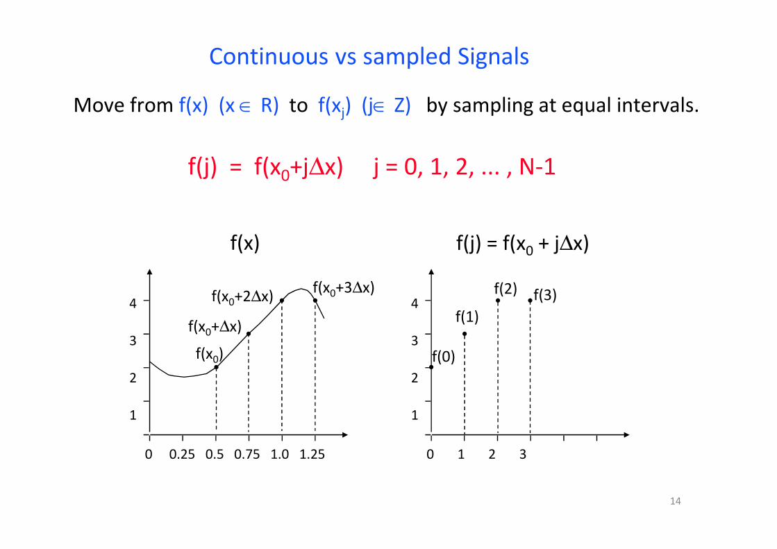
Continuous vs sampled Signals

Move from f(x) (x ∈ R) to f(xj) (j∈ Z) by sampling at equal intervals.

f(j) = f(x0+j∆x) j = 0, 1, 2, ... , N-1

4

3

2

1

0 0.25 0.5 0.75 1.0 1.25

f(x)

f(x0)

f(x0+∆x)

f(x0+2∆x)f(x0+3∆x)

4

3

2

1

0 1 2 3

f(j) = f(x0 + j∆x)

f(0)

f(3)f(2)

f(1)

15

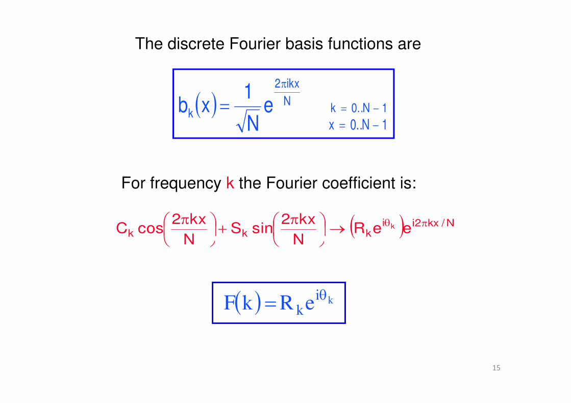
The discrete Fourier basis functions are

( ) 1N..0kN

ikx2

k eN

1xb −=

π

=

( ) N/kx2iikkk eeR

N

kx2sinS

N

kx2cosC k πθ→

π

+

π

( ) kikeRkF

θ=

1N..0x −=

For frequency k the Fourier coefficient is:

16

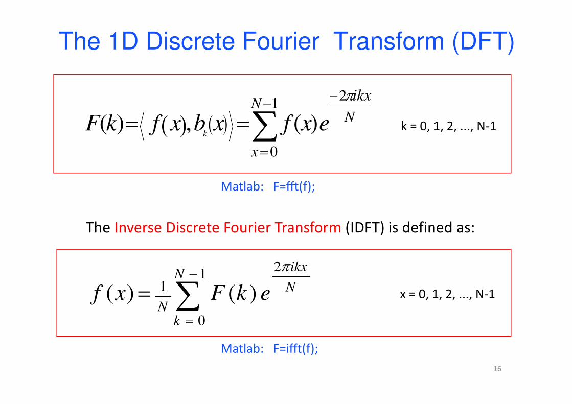
k = 0, 1, 2, ..., N-1( ) ( ) ∑−

=

−

==1

0

2

)(,)(N

x

N

ikx

exfxbxfkFk

π

∑−

=

=1

0

2

1 )()(N

k

N

ikx

NekFxf

π

x = 0, 1, 2, ..., N-1

The Inverse Discrete Fourier Transform (IDFT) is defined as:

Matlab: F=fft(f);

Matlab: F=ifft(f);

The 1D Discrete Fourier Transform (DFT)

17

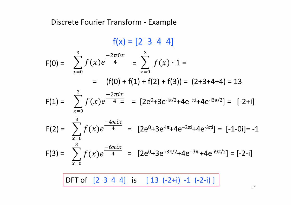
Discrete Fourier Transform - Example

F(0) =

= (f(0) + f(1) + f(2) + f(3)) = (2+3+4+4) = 13

F(1) = = = [2e0+3e-iπ/2+4e−πi+4e-i3π/2] = [-2+i]

F(3) = = [2e0+3e-i3π/2+4e−3πi+4e-i9π/2] = [-2-i]

F(2) = = [2e0+3e-iπ+4e−2πi+4e-3πi] = [-1-0i]= -1

DFT of [2 3 4 4] is [ 13 (-2+i) -1 (-2-i) ]

f(x) = [2 3 4 4]

�

����(�)������

�

����(�)�������

�

����(�)�������

�

����(�)������ = �

���� � ∙ 1 =

18

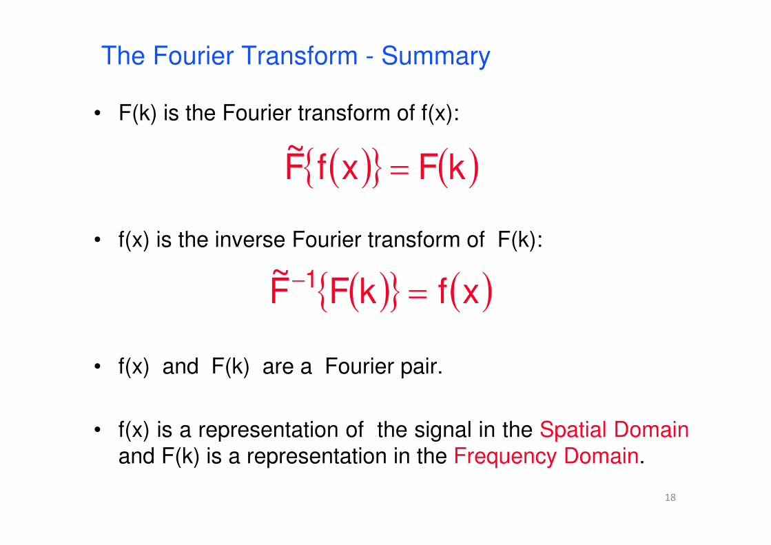
• F(k) is the Fourier transform of f(x):

• f(x) is the inverse Fourier transform of F(k):

• f(x) and F(k) are a Fourier pair.

• f(x) is a representation of the signal in the Spatial Domain

and F(k) is a representation in the Frequency Domain.

( ){ } ( )kFxfF~ =

( ){ } ( )xfkFF~ 1 =−

The Fourier Transform - Summary

19

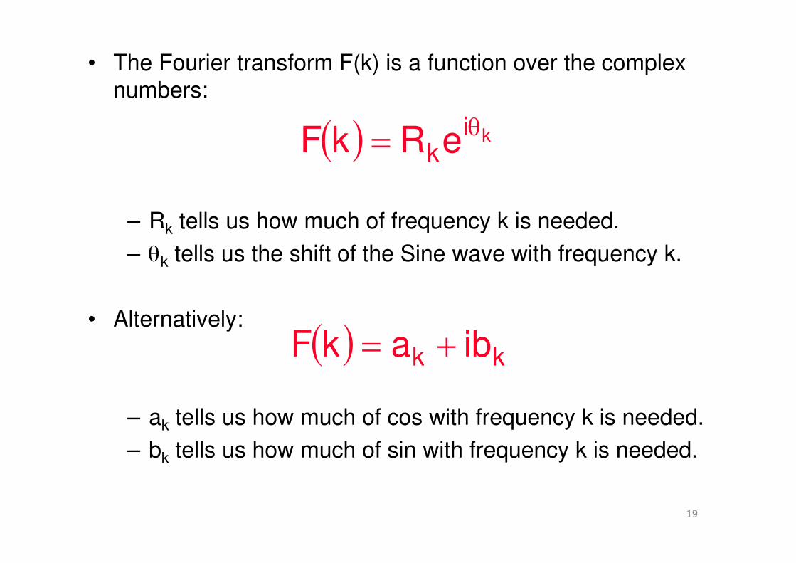
• The Fourier transform F(k) is a function over the complex

numbers:

– Rk tells us how much of frequency k is needed.

– θk tells us the shift of the Sine wave with frequency k.

• Alternatively:

– ak tells us how much of cos with frequency k is needed.

– bk tells us how much of sin with frequency k is needed.

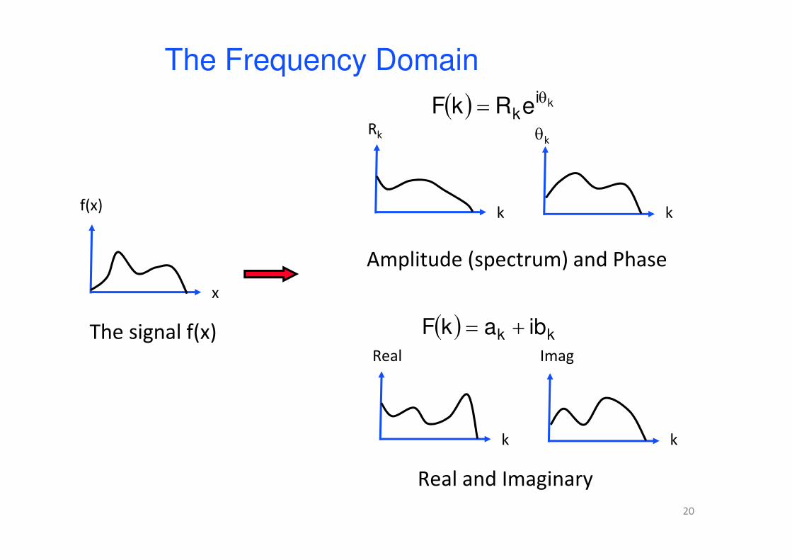
( ) kikeRkF θ=

( ) kk ibakF +=

20

x

f(x) k

Rk

k

θk

( ) kikeRkF θ=

The signal f(x)

k

Real

k

Imag

( ) kk ibakF +=

Amplitude (spectrum) and Phase

Real and Imaginary

The Frequency Domain

21

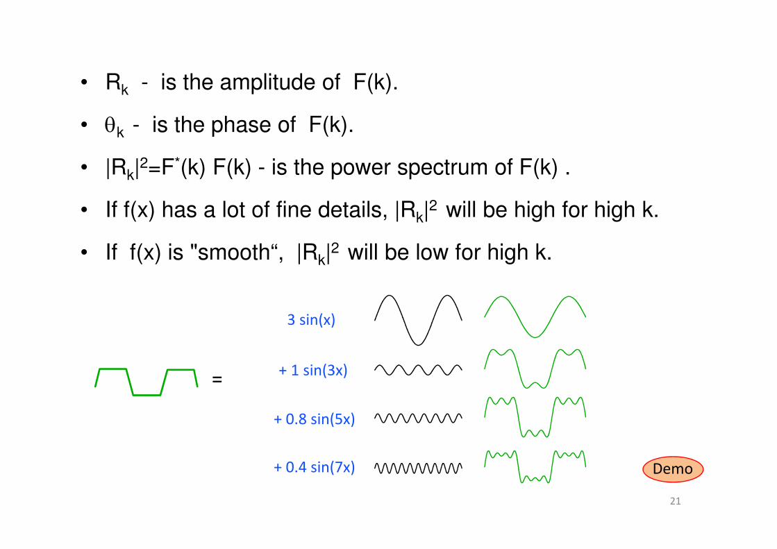
• Rk - is the amplitude of F(k).

• θk - is the phase of F(k).

• |Rk|2=F*(k) F(k) - is the power spectrum of F(k) .

• If f(x) has a lot of fine details, |Rk|2 will be high for high k.

• If f(x) is "smooth“, |Rk|2 will be low for high k.

3 sin(x)

+ 1 sin(3x)

+ 0.8 sin(5x)

+ 0.4 sin(7x)

=

Demo

22

Examples

23

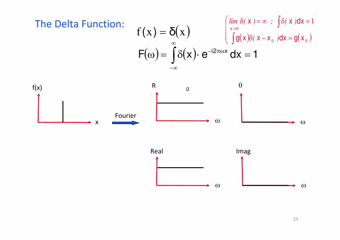
( )xxf δ)( =

( ) ( ) 1dxexF x2i =⋅δ=ω πω−∞

∞−∫

Fourierωx

f(x) R

ω

θ

ω

Imag

The Delta Function:

0

( ) ( )

=−δ

=δ∞=δ

∫∫

→

00

0

1

xgdxxxxg

dxxxx

)(

)(;)(lim

ω

Real

24

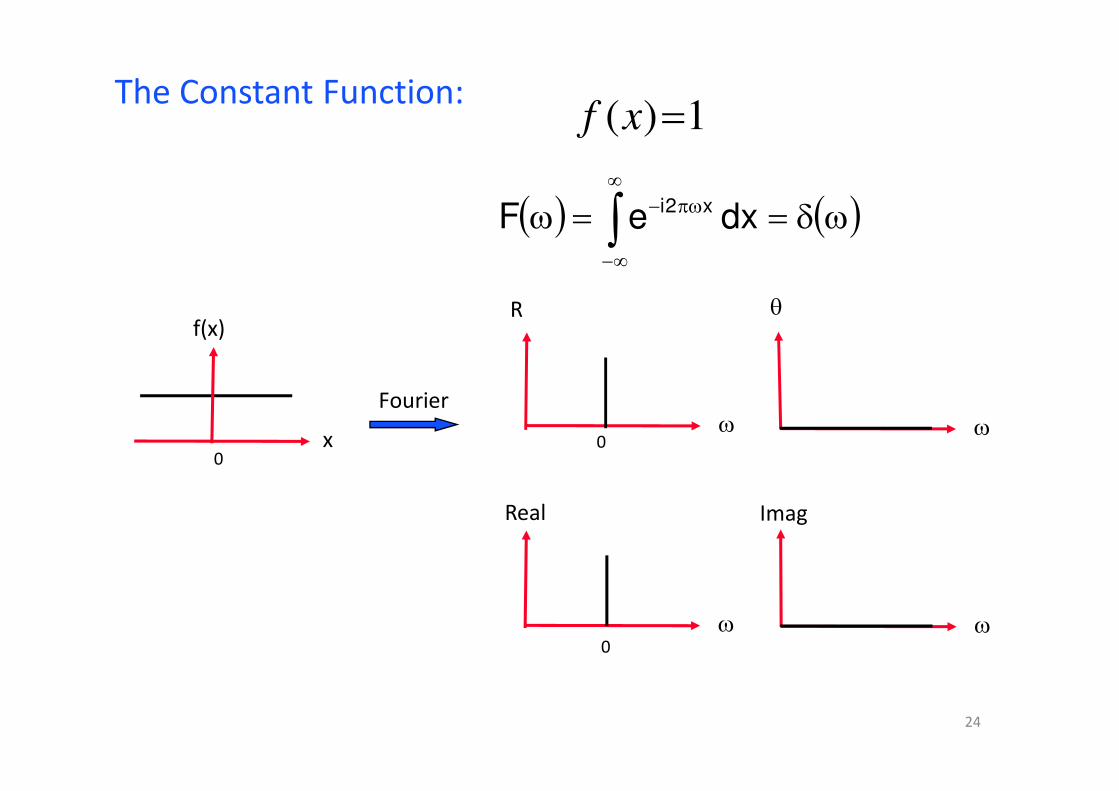
The Constant Function:1)( =xf

( ) ( )ωδ==ω ∫∞

∞−

πω− dxeF x2i

x

f(x)

0

Fourierω

R

ω

θ

0

ω

Real

ω

Imag

0

25

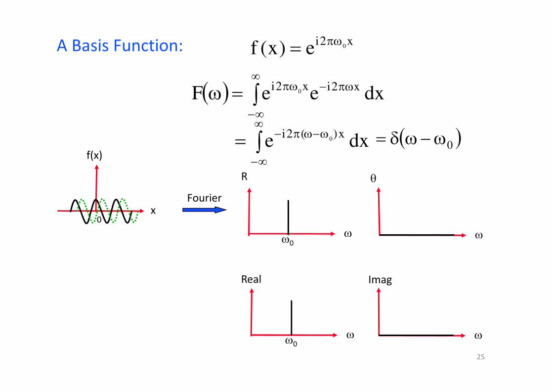
A Basis Function:

Fourier

x2i0e)x(f

πω=

( ) dxeeF x2ix2i0∫

∞

∞−

πω−πω=ω

dxex)(2i

0∫∞

∞−

ω−ωπ−= ( )0ω−ωδ=

x

f(x)

0

ω

R

ω0ω

θ

ω

Real

ω0ω

Imag

26

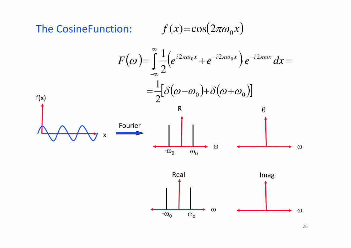
The CosineFunction:

Fourier

( )xxf 02cos)( πω=

( ) ( ) =⋅+= −∞

∞−

−∫ dxeeeFxixixi πωπωπωω 222 00

2

1

( ) ( )[ ]002

1ωωδωωδ ++−=

ω

R

ω

θ

ω0-ω0

ω

Real

ω

Imag

ω0-ω0

x

f(x)

27

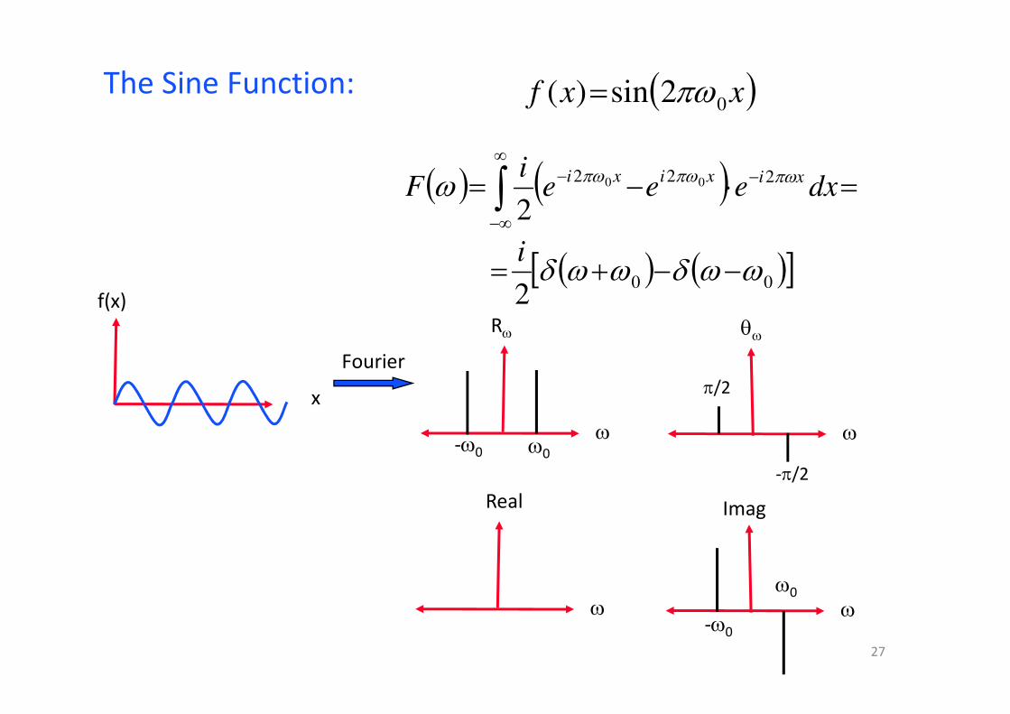
The Sine Function:

Fourier

( )xxf 02sin)( πω=

( ) ( ) =⋅−= −∞

∞−

−∫ dxeeei

Fxixixi πωπωπωω 222 00

2

( ) ( )[ ]002

ωωδωωδ −−+=i

x

f(x)

ω

Rω

ω

θω

ω0-ω0

π/2

-π/2

ω

Real

ω

Imag

ω0

-ω0

28

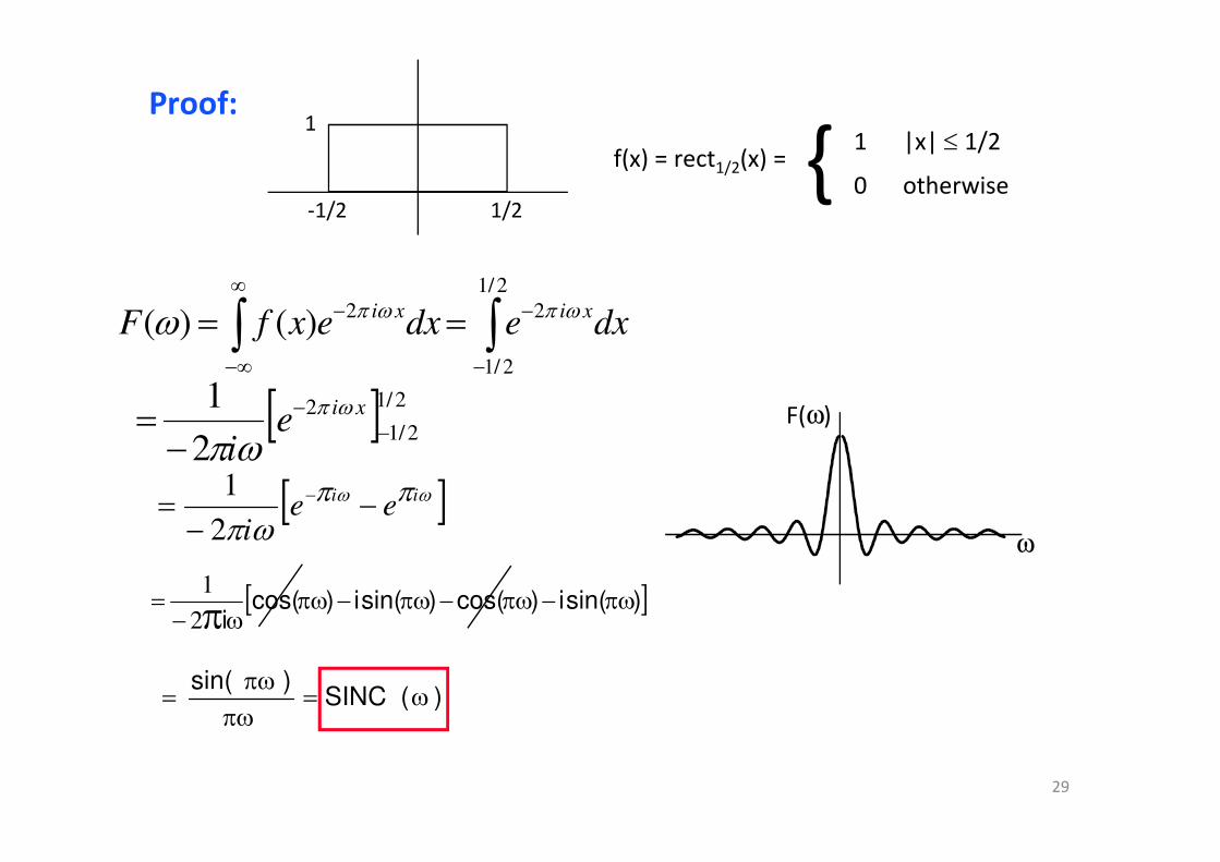
The Window Function (rect):

Fourier

<=

otherwise021if1

)(2

1

xxrect

( ) ( ) ( )πωπωπω

ω πω sincsin

5.0

5.0

2 === ∫−

−dxeF

xi

x

f(x)

-0.5 0.5

Rω

ω

29

Proof:

f(x) = rect1/2(x) = { 1 |x| ≤ 1/2

0 otherwise

1

-1/2 1/2

dxedxexfFxixi ∫∫

−

−∞

∞−

− ==2/1

2/1

22)()( ωπωπω

[ ] 2/1

2/1

2

2

1−

−

−= xi

ei

ωπ

ωπ[ ]ωω ππ

ωπii

eei

−−

= −

2

1

[ ])sin(i)cos()sin(i)cos(i

πω−πω−πω−πωω−

= π21

)(SINC)sin(

ω=πωπω

=

ω

F(ω)

30

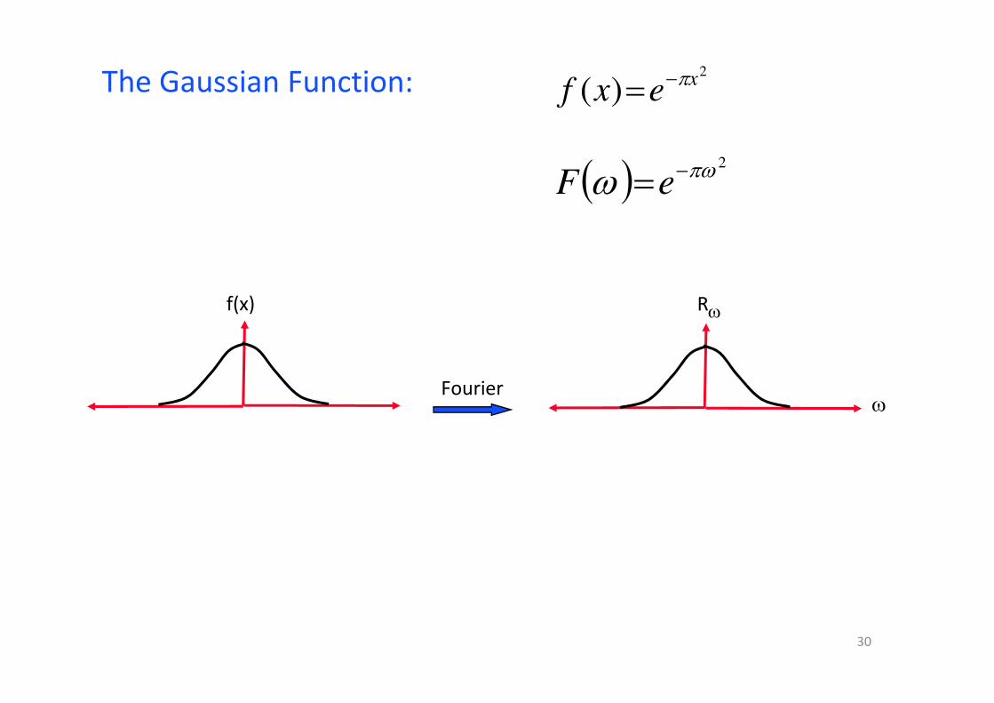
The Gaussian Function:

Fourier

2

)( xexf

π−=

( ) 2πωω −=eF

f(x) Rω

ω

31

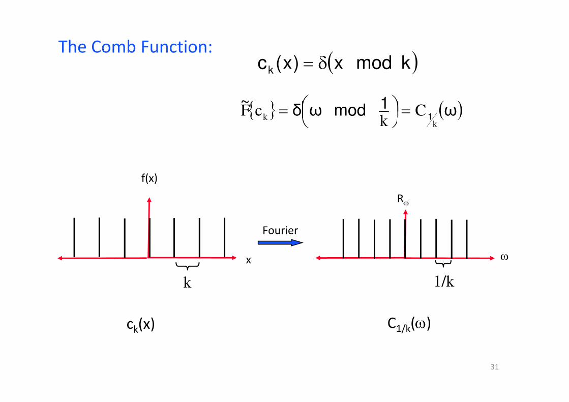
The Comb Function:

Fourier

( )kmodx)x(ck δ=

{ } ( )ω1modωδ~

1k

k Ck

cF =

=

x

f(x)

k

ck(x)

Rω

ω

1/k

C1/k(ω)

32

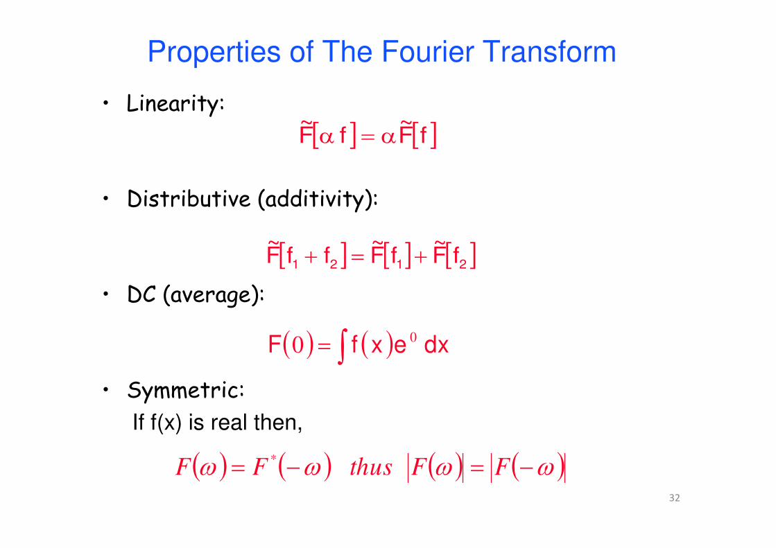
Properties of The Fourier Transform

• Linearity:

• Distributive (additivity):

• DC (average):

• Symmetric:

If f(x) is real then,

[ ] [ ] [ ]2121 fF~

fF~

ffF~ +=+

[ ] [ ]fF~

fF~ α=α

( ) ( ) ( ) ( )ωωωω −=−= FFthusFF*

( ) ( )∫= dxexfF 00

33

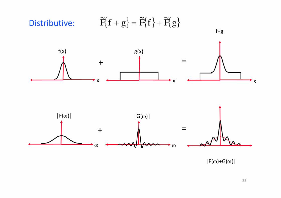
Distributive:

x

f(x)

ω

|F(ω)|

x

g(x)

ω

|G(ω)|

x

f+g

|F(ω)+G(ω)|

{ } { } { }gFfFgfF~~~ +=+

+

+ =

=

34

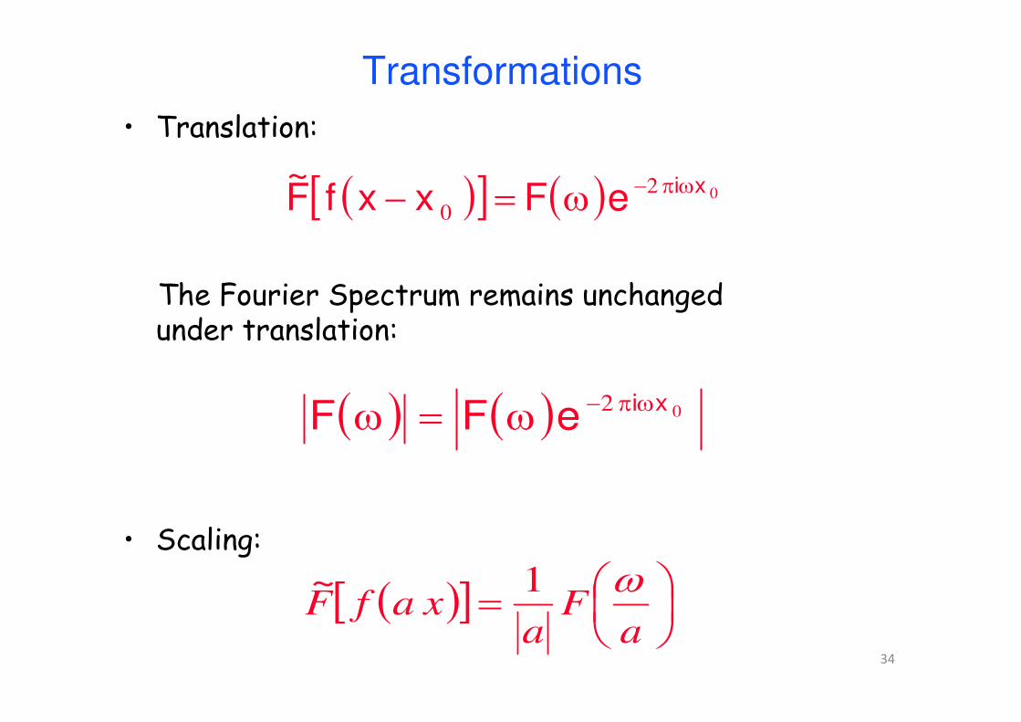
Transformations

• Translation:

The Fourier Spectrum remains unchanged under translation:

• Scaling:

( )[ ] ( ) 02

0

xieFxxfF ωπ−ω=−~

( ) ( ) 02 xieFF ωπ−ω=ω

( )[ ]

=

aF

axafF

ω1~

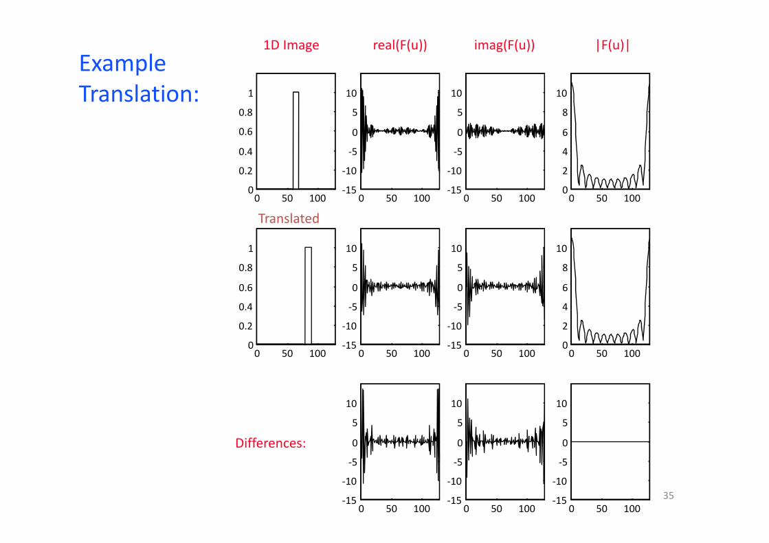
35

Example

Translation:

0 50 1000

0.2

0.4

0.6

0.8

1

0 50 1000

0.2

0.4

0.6

0.8

1

0 50 100-15

-10

-5

0

5

10

0 50 100-15

-10

-5

0

5

10

0 50 100-15

-10

-5

0

5

10

0 50 100-15

-10

-5

0

5

10

0 50 1000

2

4

6

8

10

0 50 1000

2

4

6

8

10

0 50 100-15

-10

-5

0

5

10

0 50 100-15

-10

-5

0

5

10

0 50 100-15

-10

-5

0

5

10

1D Image

Translated

real(F(u)) imag(F(u)) |F(u)|

Differences:

36

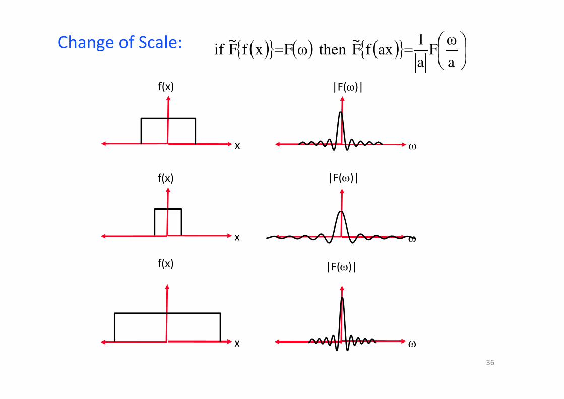
Change of Scale:

x

f(x)

ω

|F(ω)|

x

f(x)

ω

|F(ω)|

x

f(x)

ω

|F(ω)|

( ){ } ( ) ( ){ }

==a

ωF

a

1axfF

~thenωFxfF

~if

37

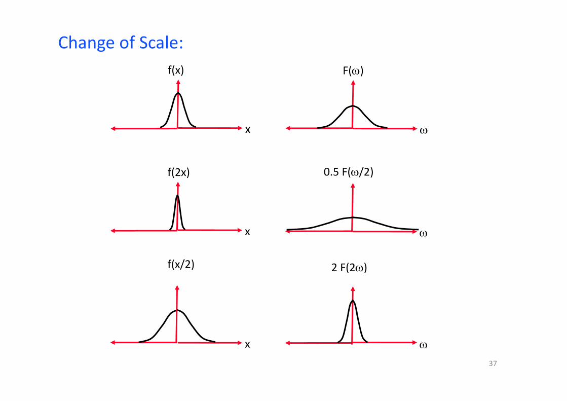
Change of Scale:

x

f(x)

ω

F(ω)

x

f(2x)

ω

0.5 F(ω/2)

x

f(x/2)

ω

2 F(2ω)

38

End