The formation of subglacial streams and mega-scale glacial ...

Proc. R. Soc. A (2010) 466, 3181–3201doi:10.1098/rspa.2010.0009

Published online 21 April 2010

The formation of subglacial streams andmega-scale glacial lineations

BY A. C. FOWLER*

MACSI, Department of Mathematics and Statistics, University of Limerick,Limerick, Republic of Ireland

The instability theory of drumlin formation has been very successful in predicting theexistence of ribbed moraine, as well as its amplitude and wavelength. However, the theoryas it stands has not yet been shown to have the capability of predicting the existenceof three-dimensional bedforms—drumlins—or their more extreme cousins, mega-scaleglacial lineations. We extend the instability theory to include a dynamic descriptionof the local subglacial drainage system, and in particular, we show that a uniformwater-film flow between ice and deformable subglacial till is unstable, and that as aconsequence, lineations will form. Predictions of the transverse wavelengths are consistentwith observations.

Keywords: mega-scale glacial lineations; megaflutes; stream formation; instability

1. Introduction

Mega-scale glacial lineations (MSGLs; Clark 1993) are very long topographicridge-groove corrugations, up to tens of metres in height, hundreds of metres inwidth and up to 100 km in length (figure 1); much longer than drumlins, whichare usually less than a kilometre in length. They were discovered on the now-exposed beds of former ice sheets, and their presence was inferred to record thelocation of ice streams (Clark 1993). This hypothesis has recently been validatedby King et al. (2009), who have found MSGLs under the Rutford ice streamin Antarctica. While it is generally agreed that MSGLs are formed through theaction of ice (although see Shaw et al. (2008) and the reply by Ó Cofaigh et al.(2010)), it is as yet unclear how they do so. The question is of practical, as wellas scientific interest, since it has a bearing on the drag that the bed offers the ice,and hence on how rapidly the ice streams discharge. In a warming climate, theseare important ingredients of the process whereby ice sheets melt or collapse andthe sea level rises.

There have been a number of suggestions as to how such lineations could beformed. Clark et al. (2003) suggest that they are formed through the ‘combing’action of basal ice as it ploughs through sediment. Schoof & Clarke (2008),following Shaw & Freschauf (1973), suggest that they may be formed through

*[email protected]

Received 7 January 2010Accepted 22 March 2010 This journal is © 2010 The Royal Society3181

on September 27, 2010rspa.royalsocietypublishing.orgDownloaded from

mailto:[email protected]

http://rspa.royalsocietypublishing.org/

3182 A. C. Fowler

Figure 1. Mega-scale glacial lineations observed on a satellite image of part of Canada. The MSGLsare the ridge-furrow corrugations of the order of 100 m in width and spacing, and up to 20 km inlength. Direction of ice flow was from right to left; note how the pattern is slightly curved.

a transverse secondary flow in basal ice, which is caused by a non-Newtonianrheology. Many have argued that ribbed moraine, drumlins, megaflutes andMSGLs are part of a continuous spectrum of bedforms (Sugden & John 1976;Aario 1977; Boulton 1987; Rose 1987; Clark 1993), with MSGLs as the upper-end member in the scale. In this view, the bed-forming mechanism provides theobserved shapes, depending on the local ice-flow conditions. Most obviously, onemight suppose that the transition from ribs to drumlins to lineations occurs asthe ice flow increases.

The instability theory of drumlin formation (Hindmarsh 1998; Fowler 2000,2009; Schoof 2007a; Dunlop et al. 2008) is the first theory that is able tosuccessfully predict qualitative characteristics of drumlinoid topography, suchas amplitude and wavelength, on the basis of a physically based mathematicalmodel. As such, its adherents might expect that the theory would provide thebuilding blocks for all the main types of bedforms that are observed. However, thisappears not to be so. In particular, Schoof (2007a) pointed out three difficultieswith the theory. The first is that almost as soon as the bedforms begin to grow,cavities form on their lee. In a later paper, Schoof (2007b) finds that thereare finite-amplitude travelling wave solutions, whose elevation scales with thedeforming till thickness. Since this is most probably of the order of centimetresto metres, it apparently mitigates against observations of drumlins of tens ofmetres elevation (although, in fact, the average elevation of drumlins is actuallyabout 7 m; Clark et al. 2009). This difficulty was potentially resolved by Fowler(2009), who showed that finite-amplitude bedforms of appropriate amplitudecould indeed be obtained, even when cavities were present. However, Fowler’sformulation of the problem is different from Schoof’s, and relies on a plausiblebut heuristic assumption that cavities are infilled by sediments, in the manner ofcrag and tail landforms.

Proc. R. Soc. A (2010)



Mega-scale glacial lineations 3183

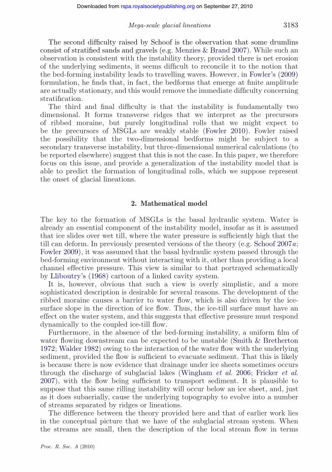
The second difficulty raised by Schoof is the observation that some drumlinsconsist of stratified sands and gravels (e.g. Menzies & Brand 2007). While such anobservation is consistent with the instability theory, provided there is net erosionof the underlying sediments, it seems difficult to reconcile it to the notion thatthe bed-forming instability leads to travelling waves. However, in Fowler’s (2009)formulation, he finds that, in fact, the bedforms that emerge at finite amplitudeare actually stationary, and this would remove the immediate difficulty concerningstratification.

The third and final difficulty is that the instability is fundamentally twodimensional. It forms transverse ridges that we interpret as the precursorsof ribbed moraine, but purely longitudinal rolls that we might expect tobe the precursors of MSGLs are weakly stable (Fowler 2010). Fowler raisedthe possibility that the two-dimensional bedforms might be subject to asecondary transverse instability, but three-dimensional numerical calculations (tobe reported elsewhere) suggest that this is not the case. In this paper, we thereforefocus on this issue, and provide a generalization of the instability model that isable to predict the formation of longitudinal rolls, which we suppose representthe onset of glacial lineations.

2. Mathematical model

The key to the formation of MSGLs is the basal hydraulic system. Water isalready an essential component of the instability model, insofar as it is assumedthat ice slides over wet till, where the water pressure is sufficiently high that thetill can deform. In previously presented versions of the theory (e.g. Schoof 2007a;Fowler 2009), it was assumed that the basal hydraulic system passed through thebed-forming environment without interacting with it, other than providing a localchannel effective pressure. This view is similar to that portrayed schematicallyby Lliboutry’s (1968) cartoon of a linked cavity system.

It is, however, obvious that such a view is overly simplistic, and a moresophisticated description is desirable for several reasons. The development of theribbed moraine causes a barrier to water flow, which is also driven by the ice-surface slope in the direction of ice flow. Thus, the ice-till surface must have aneffect on the water system, and this suggests that effective pressure must responddynamically to the coupled ice-till flow.

Furthermore, in the absence of the bed-forming instability, a uniform film ofwater flowing downstream can be expected to be unstable (Smith & Bretherton1972; Walder 1982) owing to the interaction of the water flow with the underlyingsediment, provided the flow is sufficient to evacuate sediment. That this is likelyis because there is now evidence that drainage under ice sheets sometimes occursthrough the discharge of subglacial lakes (Wingham et al. 2006; Fricker et al.2007), with the flow being sufficient to transport sediment. It is plausible tosuppose that this same rilling instability will occur below an ice sheet, and, justas it does subaerially, cause the underlying topography to evolve into a numberof streams separated by ridges or lineations.

The difference between the theory provided here and that of earlier work liesin the conceptual picture that we have of the subglacial stream system. Whenthe streams are small, then the description of the local stream flow in terms




3184 A. C. Fowler

x

= iice surface

substratum

= s h

Figure 2. Schematic representation of model geometry. Ice with surface z = zi lies above the till;where the effective stress at the base reaches zero, there is also a water layer of depth h.

of a locally defined effective pressure makes sense (Röthlisberger 1972), and weregain the earlier theory (Schoof 2007a; Fowler 2009). A different viewpoint,which we might call ‘wide stream theory’, does not distinguish the scale of thestream flow from that of the ice, and thus the streams become indistinguishablefrom cavities, with their depth being controlled by the criterion that the effectivepressure at the ice–water interface is zero. The only difference is that cavitiesare formed through the deficit pressures generated by ice flow, whereas streamsare caused by the excess pore pressures generated by permeable flow through thetill. As we shall see, from a mathematical point of view, small stream theory is aparticular case of wide stream theory. Our view of the subglacial stream systembears resemblance to the experimental results of Catania & Paola (2001), andour theoretical description of subglacial water flow is similar to that of Le Brocqet al. (2009), although they do not include a dynamic dependence of the waterpressure on the ice flow.

The geometry of the flow we consider is indicated in figure 2. We take axes(x , y, z), with z vertically upwards and x pointing in the direction of ice flow.The ice surface is denoted by z = zi. We define N to be the effective stress at thebase of the ice, which we take to be at z = s. If N > 0, then ice is assumed to reston the underlying wet till, while if N reaches zero, then a water film or streamor cavity of depth h is formed. In general, the bed will thus consist of two parts:attached, where N > 0 and h = 0; and separated, where N = 0 and h > 0. We nowwish to describe the water flow in each regime.

We define a number of different pressures: pw is the water pressure at the icebase z = s; pT is the pressure in the till; and pi is the ice pressure, and in theusual way for ice flow, we subtract the cryostatic component by writing

pi = pa + rig(zi − z) + P, (2.1)

where pa is atmospheric pressure, ri is the density of ice, g is the acceleration dueto gravity and we call P the reduced pressure. Fowler (2010) showed that therelaxation time of the pore pressure in the till was rapid, and so we suppose that





the pore pressure p in the till is hydrostatic,

p = pw + rwg(s − z), (2.2)

where rw is the density of water. If s is the stress tensor in the ice, then theeffective stress at the ice base is

N = −snn − pw, (2.3)

where n is the unit normal (upwards, say) at the interface. The effective pressurein the till is denoted by pe, and can be determined to be (using the fact thatpT = −snn at z = s)

pe = pT − p = N + DrTwg(s − h − z), (2.4)

whereDrTw = (rs − rw)(1 − f), (2.5)

rs is the sediment density and f is the till porosity. Strictly, equation (2.4) assumesthat f is constant, which is probably a reasonable approximation; relation (2.4)applies at both attached and separated parts of the base.

The hydraulic head at the ice base is pw + rwgs, and it is convenient to add aconstant, thus we define the hydraulic head to be

j = pw + rwgs − (pa + rigdi), (2.6)

where di is the local ice depth (at x = 0). This is not the same as zi because weallow for a small ice-surface slope to drive both ice and water flow. The deviatoricstress tensor is defined by

s = −pid + t, (2.7)

where d is the unit tensor, and it follows from this that

N = rig(zi − di) + Drwigs + P − tnn − j, (2.8)

whereDrwi = rw − ri. (2.9)

This determines N in terms of ice flow and hydraulic gradient.

(a) Groundwater flow

In general, water is formed at the base through basal melting at typical ratesof millimetres per year, and this water provides a flux that must be evacuated,essentially in the direction of ice flow. If h = 0, then we suppose water flowsthrough the till and underlying sediments by Darcian flow.

The porosity should be a function of the local effective pressure in the till,thus f = f(pe), while the local water flux is given by −(k/hw)Vj, where k is thepermeability and hw is the viscosity of water. Here and below, V is the horizontalgradient operator (v/vx , v/vy). If we assume a vertical hydrostatic equilibrium for




3186 A. C. Fowler

the pore water (Fowler 2010), then j does not vary vertically. Then, the waterflux integrated over a column of till is

Q = − 1hw

(∫ s

0k dz

)Vj. (2.10)

Conservation of water mass then takes the formv

vt

∫ s

0f dz + V · Q = 0, (2.11)

if we ignore the local melt production term. The justification for this is that thewater flux arises through basal melting over ice-sheet length scales li ∼ 106 m,whereas we are concerned with the bedform length scales l ∼ 102–103 m, so thatthe relative size of the melting term in equation (2.11) to the flux divergence termwill be ∼ (l/li) # 1.

To find a simple form of this equation, suppose that the variations of s, f andk are small. Then, f ≈ f(N ) + f′DrTg(s − z), and if the variation in s is a gooddeal less than the depth of the permeable sediments, then equation (2.11) can bewritten approximately as

f′Nt + DrTgf′st = V ·(

khw

Vj

). (2.12)

If, however, the depth of the aquifer was constant, for example being the depthof deformable till, then the term in st would be absent. More generally, we mightinclude this term, but with a smaller coefficient than in equation (2.12).

(b) Stream/cavity flow

When the ice separates from the till, water can flow through the resultingchannel, whether this be a stream or a cavity. Assuming laminar flow, the waterflux is (Batchelor 1967)

J = − h3

12hwVj, (2.13)

and mass conservation then takes the form

ht + V · J = 0. (2.14)

In fact, there will still be water flow through the till, and the total mass-flowequation should include this, but as we shall see, the flux through a stream isvery much larger than that in the till, so that one can reasonably ignore it.

(c) Sediment flux

The sediment flux owing to the deformation of till has been described by Fowler(2010). It has two elements. The motion of the ice at the interface exerts a dragon the till, and this will cause a mechanical deformation and consequent sedimentflux. Quite how this depends on the sliding velocity ub will depend on the choiceof till rheology. As a saturated granular material, till has a plastic yield stress, butthis statement is not sufficient to determine the flow behaviour (Fowler 2003).Plausible flow rules (e.g. Iverson & Iverson 2001; Jop et al. 2006) suggest aneffective viscous behaviour, and a resulting Couette-type flow would have the





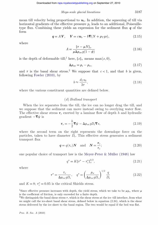
mean till velocity being proportional to ub. In addition, the squeezing of till viahorizontal gradients of the effective pressure pe leads to an additional, Poiseuille-type flux. Combining these yields an expression for the sediment flux q of theform

q = AV , V = cub − bV(N + rTgs), (2.15)

where

A = [t − mN ]+mDrswg(1 − f)

(2.16)

is the depth of deformable till;1 here, [x]+ means max(x , 0),

Drsw = rs − rw, (2.17)

and t is the basal shear stress.2 We suppose that c < 1, and that b is given,following Fowler (2010), by

b ≈ dTu0

3t, (2.18)

where the various constituent quantities are defined below.

(d) Bedload transport

When the ice separates from the till, the ice can no longer drag the till, andwe suppose that the sediment can move instead owing to overlying water flow.The effective shear stress te exerted by a laminar flow of depth h and hydraulicgradient −Vj is

te = −h2

Vj − DrswgDsVs, (2.19)

where the second term on the right represents the downslope force on theparticles, taken to have diameter Ds. This effective stress generates a sedimenttransport flux

q = q(te)N and N = te

te; (2.20)

one popular choice of transport law is the Meyer-Peter & Müller (1948) law

q∗ = K [t∗ − t∗c ]3/2

+ , (2.21)

where

t∗ = te

DrswgDs, q∗ =

(rw

DrswgDs

)1/2 qDs

(2.22)

and K = 8; t∗c = 0.05 is the critical Shields stress.

1Since effective pressure increases with depth, the yield stress, which we take to be mpe, where mis the coefficient of friction, is only exceeded for a finite depth.2We distinguish the basal shear stress t, which is the shear stress at the ice–till interface, from whatwe might call the ice-sheet basal shear stress, defined below in equation (2.34), which is the shearstress delivered by the ice sheet to the basal region. The two would be equal if the bed was flat.




3188 A. C. Fowler

(e) Stream- and sediment-flow models

Summarizing, we have two equations for stream flow and sediment flow. Thesecond of these is the Exner equation. For attached flow, N > 0 and h = 0, we have

f′(Nt + raDrTwgst) = V ·[

khw

Vj

]

and st + V · [A{cub − bV(N + DrTwgs)}] = 0,

(2.23)

where f′ = f′(pe) is the derivative of f with respect to effective pressure and ra is anumber representing the aquifer depth: ra = 1 for a full aquifer in 0 < z < s, whilera = 0 for an aquifer of fixed depth; generally we may suppose that 0 ≤ ra ≤ 1.

For separated flow, where N = 0 and h > 0, we have

ht = V ·[

h3

12hwVj

]

and st − ht + V · [q(te)N ] = 0

(2.24)

(note that the till–water interface is at z = s − h). These equations determine sand N , and s and h, respectively; j is defined by equation (2.8), and the stream-and sediment-flow models are coupled to the ice flow through the normal stressterm in equation (2.8).

(f ) Ice-flow model

The ice-flow model has been described frequently before (Hindmarsh 1998;Fowler 2000; Schoof 2002, 2007a; Fowler 2009, 2010), and is only summarizedhere. We follow Fowler’s (2010) exposition, which assumes flow of Newtonianviscous ice over the bed, as shown in figure 2. The ice base is at z = s and the(gently sloping) ice surface is at z = zi. When written in terms of the reducedpressure P, the Stokes equations take the form

V · u = 0

and 0 = −VP − rigVzi + hiV2u,

}

(2.25)

where u is the ice velocity, and hi is the ice viscosity. Kinematic boundaryconditions are applied at the top and bottom (ignoring both surfaceaccumulation/ablation and basal melting), which describe the time evolution ofeach surface in terms of the normal velocity of the ice. These conditions specifythat ice particles in the surface remain there. In addition, we prescribe boundaryconditions of continuous stress across the top surface, and no normal velocity atthe base, together with a sliding law there of the form

t = f (ub, N )ub

ub, (2.26)

where t is the basal traction.





(g) Non-dimensionalization

The equations are non-dimensionalized in the manner devised by Schoof(2007a), as modified by Fowler (2009). We define an effective pressure scale Nc(which will be chosen later). Three relevant length scales are then

dD = Nc

Drwig, (2.27)

which is a measure of bedform elevation;

dT = Nc

Drswg(1 − f), (2.28)

which is a measure of deforming till depth; and

l =(

hiu0

Drwig

)1/2

, (2.29)

which is a suitable horizontal length scale for bedforms; here, u0 is the horizontalvelocity scale, which is determined from the sliding law. Since MSGLs have typicalwidths of the order of hundreds of metres, it is reasonable to expect that l (whichhas a similar order of magnitude) is appropriate. It should be emphasized thatthis choice of scale does not affect the following analysis.

In a basic uniform state where s = 0, P = 0 and the ice surface has a downwardslope S in the x-direction, there is a basic shear flow for the ice given by

u =[u0 + tb

hi

(z − z2

2di

)]i, (2.30)

where

tb = rigdiS (2.31)

is the basal shear stress of the underlying ice flow; i is the unit vector in thex-direction3. The equations are scaled by choosing

s ∼ dD, x ∼ l , j, N , P, tnn , t, f ∼ Nc, te ∼ DrswgDsdD

l,

zi = dihi, A ∼ dT, h ∼ h0, q ∼ u0dT,

u −[u0u + tb

hi

(z − z2

2di

)]i ∼ dDu0

land t ∼ t0 = dDl

dTu0;

(2.32)

the film-thickness scale is chosen to balance a presumed upstream water fluxQ0, itself derived from a typical melt rate m over a typical catchment length li.

3It should be noted that although this does not exactly satisfy the top-surface boundary conditions,it is an accurate approximation for small surface slopes S .




3190 A. C. Fowler

If we take m ∼ 1 mm yr−1 and li ∼ 1000 km, then Q0 ∼ 103 m2 yr−1. The choice ofh0 is then

h0 =(

12hwlQ0

Nc

)1/3

. (2.33)

A number of parameters are introduced in non-dimensionalizing. In particular,we define

n = dD

l, s = l

diand q = tb

Nc. (2.34)

These represent the aspect ratio of the lower surface (n) and the ‘corrugation’of the lower surface (s). The value of the parameter q depends on the choiceof the effective pressure scale Nc. Previously (Fowler 2009), this was chosen asthe prescribed channel effective pressure scale. In the current context, there maybe no prescribed Nc, and it is then natural to choose Nc = tb, and thus q = 1,which we now do. The dimensionless ice depth hi is defined in terms of a surfaceperturbation H by writing

hi = 1 − sSx + SH , (2.35)

which points out the role of the mean slope of the ice surface.Central to the solution of the ice-flow problem is the assumption that the aspect

ratio is small. This allows us to linearize the geometry to a half space, as wellas linearizing the geometric nonlinearities in the stress and velocity components.With this simplification, we find that the ice velocity is uniform at leading order,u ≈ u(t)i, and thus the leading order form of the dimensionless sliding law is

t = f (u, N ), (2.36)

and u is defined by the requirement that the average stress be equal to one, i.e.

1 = f (u, N ), (2.37)

where the overbar denotes a space average.The dimensionless normal compressive stress at the base is written as

P − tnn = −H − Q, (2.38)

and then the dimensionless hydraulic gradient is

j = −sx + s − Q − N . (2.39)

The surface perturbation H satisfies the approximate equation derived from thekinematic condition

lHt = X, (2.40)

which equates the ice-surface motion to the vertical ice velocity (= X), and thequantities Q and X are determined in terms of the quantities H , K and F , wherethe latter two are defined by

K = ast + usx and F = f (u, N ) − 1. (2.41)

The determination of Q and X is described by Fowler (2010). The Fouriertransforms of Q and X are given by linear combinations of those of H , K and F .





Table 1. Typical values of the dimensional constants in the model. The ice viscosity is calculatedusing Paterson’s (1994) recommended value of the flow-law coefficient at 0◦C and a stress of0.6 × 105 Pa. See text for further explanation.

symbol meaning typical value

ri ice density 917 kg m−3

DrTw till–water density difference (2.5) 103 kg m−3

rw water density 103 kg m−3

di ice depth 103 mDrwi equation (2.9) 83 kg m−3

g gravity 9.8 m s−2

k permeability 10−15 m2

hw water viscosity 1.8 × 10−3 Pa sf porosity 0.4b squeeze coefficient (2.18) 0.4 × 10−2 m2 Pa−1 yr−1

c shearing coefficient (2.15) <1m coefficient of friction 0.6Drsw equation (2.17) 1.6 × 103 kg m−3

Ds grain size 10−4 mK Meyer-Peter and Müller coefficient 8Q0 meltwater flux 103 m2 yr−1

t∗c critical Shields stress 0.05

f′ derivative of f −10−7 Pa−1

hi ice viscosity 2 × 1013 Pa stb basal shear stress (2.31) 104 PaS ice-surface slope 10−3

The additional dimensionless parameters arising from the ice-flow solution are

l = (Drwi)2

riDrsw(1 − f)and a = dT

dD. (2.42)

Typical values are given below using the estimates of dimensional quantities intable 1.

(h) Stream and sediment flow

The equations for stream and sediment flow, equations (2.23) and (2.24), takethe following dimensionless form, taking into account the small aspect ratio.For attached flow where N > 0,

Nt + r ′′st = −GV2j

and st + V · [A{cui − bV(N + r ′s)}] = 0,

}

(2.43)

where

A =[

t

m− N

]

+. (2.44)




3192 A. C. Fowler

Table 2. Typical values of the scales and dimensionless parameter values, using theestimates in table 1.

symbol definition typical value

l length scale (2.29) 279 mNc = tb stress scale (2.31) 104 PadD drumlin-depth scale (2.27) 12.3 mdT till-depth scale (2.28) 1.06 mh0 water-film thickness (2.33) 2.67 mmu0 ice velocity 100 m yr−1

t0 time scale 32.4 yra equation (2.42) 0.086l equation (2.42) 0.78 × 10−2

n equation (2.42) 4.4 × 10−2

s equation (2.42) 0.28G equation (2.46) 0.073r ′ equation (2.46) 12.05r ′′ equation (2.46) ≤ r ′

ra aquifer parameter equation (2.23) ∈ [0, 1]3 equation (2.46) 2.3 × 10−5

b (1/3)an 1.26 × 10−3

k equation (2.46) 0.087d equation (2.46) 0.38 × 10−3

g equation (2.46) 0.69t∗ equation (2.46) 1.13

For separated flow, where N = 0 and h > 0, we have

3ht = V · [h3Vj],st = dht − V · [qN ],

N = te

te, q = k[te − t∗]3/2

+

and te = −Vs − ghVj.

(2.45)

The parameters G, r ′, b, 3, k, d, g and t∗ are defined by

G = kDrsw(1 − f)hw |f′| lu0Drwi

, r ′ = DrTw

Drwi, r ′′ = rar ′, b = bNc

u0l,

3 = h0dTu0

dDQ0, k = (nDs)3/2 K

u0dT

(Drswg

rw

)1/2

,

d = h0

dD, g = Drwih0

2DrswDsand t∗ = t∗

c ldD

.

(2.46)

In table 1 we give values of the dimensional constants that appear in themodel, and in table 2, we derive the corresponding scales and typical values ofthe dimensionless parameters. In comparison with the scales of Fowler (2009),





the primary difference is the choice of stress scale of 104 Pa, compared with4 × 104 Pa. More importantly, we retain the ice viscosity value of 2 × 1013 Pa sused by Fowler (2009) and Schoof (2007a). Most easily, this is explained byusing Paterson’s (1994) recommended values for Glen’s flow law of n = 3 andA = 6.8 × 10−24 Pa−3 s−1, together with a stress of 6 × 104 Pa. However, there isnothing sacrosanct about these values. One might suppose that for a stress of104 Pa, one should choose a higher viscosity of 0.7 × 1015 Pa s, but it is generallythought that at lower stress, the Glen exponent is reduced (or A increases), whichwould result in no such increase. In addition, it is known that basal ice flow oversmall slope topography causes an enhancement of stress (Fowler 1981) by a factorinverse to the slope magnitude. For both these reasons, we suppose that the lowerviscosity may be the more appropriate one.

(i) A reduced model

Suppose that h = 0 everywhere, so that the ice remains adjacent to the till. Ina steady state, we must have the water flux Q = Q0i, and when this is written indimensionless terms, it is

−Vj = Ui, (2.47)

whereU = hwlQ0

dDkNc. (2.48)

Using the estimates in tables 1 and 2, we find U ∼ 1.3 × 105. This large valueimplies that it is not possible for permeable drainage through till to evacuatesubglacial meltwater. Consequently, we suppose that some kind of stream systemmust always exist.

It is a matter of conjecture what form such a stream system should take.One simple possibility is that the high pressure generated by forcing the waterthrough the till will simply evacuate a sufficient number of fine particles to raisethe permeability to the level where it can transmit the water. This would occurthrough piping in the till. However, it is much more probable that such ‘piping’would occur at the weak ice–till interface, thus forming a film of water somemillimetres deep. This causes a conceptual difficulty, if we think of till as a fine-grained continuum. For one thing, Walder (1982) showed that such a film wouldbe unstable (at least for ice flow over hard beds). This is not in itself a problem,insofar as we are endeavouring to find a comparable instability when the ice flowsover a deformable bed, but the typical generalized Weertman sliding law of thedimensionless form

t = uAN B (2.49)

implies that the shear stress becomes zero when the effective pressure reacheszero, and this raises a difficulty, insofar as we assume that the ice delivers a finitebasal stress to the bed. We can resolve this conundrum if we relinquish the ideathat the granularity of the till is finer than the water-film depth. If the effectof the high water pressures is to wash out particles of silt size, then we mayconceptually suppose that the residual clast fraction of the till is able to providea resistance to the ice. In this view, the till provides a resistance even when theeffective pressure is zero, and the stress only decreases to zero when the water-filmthickness reaches a certain value, perhaps of the order of centimetres, depending




3194 A. C. Fowler

on the granulometry of the till. At present, we assume that this is the case. This isbasically the view of Creyts & Schoof (2009), who have explicitly studied modelsof water-film flow below ice supported by larger clasts. An alternative point ofview would allow the effective permeability of the till to increase dramatically asN approaches zero.

In this case, a uniform state consists of a water film of constant thickness abovea flat bed, and we can consider the basic model to consist of a separated flow,given by equations (2.45). Now we adopt the limits 3 → 0, d → 0, so that thereduced model for stream and sediment flow is (with N = 0)

j = −sx + s − Q,

V · [h3Vj] = 0,st = −V · [qN ],

N = te

te, q = k[te − t∗]3/2

+

and te = −Vs − ghVj.

(2.50)

3. Stability analysis

We now wish to consider the stability of a uniform state in which there is aconstant-thickness water film. By choice of the scale for h, the dimensionlesswater flux upstream is −h3Vj = i, and thus the basic uniform water flow over aflat till bed is given by

h = 1s1/3 , j = −sx , s = 0 and te = s2/3gi. (3.1)

The quantities Q in equation (2.50) and X in equation (2.40) are determined bythe perturbed ice flow: Q is (minus) the perturbed normal stress at the ice–tillinterface, while X is the normal velocity of the ice surface. Both quantities arezero in the basic state of the uniform flow. Since it is known (Schoof 2007a) thatthe ribbing instability is explicitly due to the dependence of the till flux on N , andmore particularly through the increasing dependence of the basal shear stress onN in the sliding law, we choose to suppress this dependence in order to highlightthe rilling instability present in equation (2.50). In keeping with our discussion inthe preceding section, we may do this in the present instance by taking a slidinglaw of the dimensionless Weertman form

t = f (u, N ) = uA, (3.2)

which explicitly suppresses the dependence on N . It then follows fromequation (2.37) that u = 1, and from equation (2.41), that F = 0. We assumethat l # 1 in equation (2.40), so that X = 0. We then find from Fowler (2010)that the Fourier transform Q is given by

Q = −kMK , (3.3)





0

1

2

3

4

5

1 2 3 4 5

M

ξ

Figure 3. The function M (x) given by equation (3.5).

where the Fourier transform of g(x , y) is defined by

g =∫∞

−∞

∫∞

∞g(x , y)eik1x+ik2y dx dy, (3.4)

k = |k| = |(k1, k2)|, and

M = M(

ks

)= 1

Z

[(a1a2 − a3a4)(R+ − R−)2 + a1 + a4

]; (3.5)

the coefficient functions in equation (3.5) are defined by Fowler (2010). Figure 3shows a graph of M (x), x = (k/s). M is positive, with M (∞) = 2, M ∼ (4/x) asx → 0.

To study the stability of the basic state, we write

j = −sx + J and h = 1s1/3 + h, (3.6)

and consider J, h and s to be small. Linearization of the model then leads to theequations

hx = 13s4/3 V2J

and st = − q ′0g

3s1/3 V2J + q ′0

(sxx + g

s1/3 Jxx

)+ q0

s2/3g

(syy + g

s1/3 Jyy

),

(3.7)

where

q0 = q(t0), q ′0 = q ′(t0) and t0 = s2/3g. (3.8)

The equations (3.7) are obtained after some algebra, which is omitted here, butis very similar to that involved in studying the Smith–Bretherton overland flow




3196 A. C. Fowler

model (Fowler et al. 2007). From equations (2.50), (3.3) and (2.41), we have

J = s[1 + aSMk − ik1kMu], (3.9)

where we assume an exponential time dependence, s ∝ exp(St). Substituting thisin equation (3.7)2, we find that

S = r + ikc, (3.10)

where r is the growth rate and c is the wave speed, and these are given by

c = − uEk1M1 − aEkM

and r = −D + E1 − aEkM

, (3.11)

where

D = q ′0k

21 + q0k2

2

t0and E = g

s1/3

[(q ′0

3− q0

t0

)k22 − 2

3q′0k

21

]. (3.12)

We now wish to examine equation (3.11) for conditions of instability. We notefirstly that if E < 0, then the steady state is stable. This is, for example, true forthe case where the critical Shields stress is zero, t∗

c = 0. Secondly, D increases andE decreases with k1, so that transverse (rib-like) wave components are stabilizing.Indeed, purely transverse waves are stable. This is the antithesis of the resultfrom the instability theory when the drainage is considered to be passive. Sincelongitudinal rolls are the most unstable, we now put k1 = 0; then we have k = k2,and we find that the wave speed c = 0, and the growth rate is

r‖ = (E∗ − (q0/t0))k2

1 − aE∗Mk3 , (3.13)

where

E∗ = g

s1/3

(q ′0

3− q0

t0

). (3.14)

Now let us take the Meyer-Peter and Müller choice in equation (2.45),

q(t) = k [t − t∗]3/2+ . (3.15)

Inserting this in equation (3.14), we find

E∗ = k(t0 − t∗)1/2[2t∗ − t0]2s

, (3.16)

and thus E∗ > 0 and instability is possible if t∗ < t0 < 2t∗. More precisely, we findthat E∗ > (q0/t0) if

t∗ < t0 < t+ = t∗ +(t∗2 + s2)1/2 − s. (3.17)

In this case, r‖ is positive for 0 < k < k⊥, where the critical wave number isgiven by

k⊥ =(

1aE∗M

)1/3

; (3.18)





this defines k⊥ implicitly (and uniquely), since M = M (k/s), and k3M is amonotonically increasing function. At k = k⊥, the growth rate is infinite, andfor k > k⊥, it is negative.

If, on the other hand,t+ < t < 2t∗, (3.19)

then r is positive for k > k⊥. In both cases, the most rapid (infinite) growth rateoccurs at k = k⊥, and this then provides the natural expected wavenumber forthe patterns we should expect to see.

4. Discussion

The equations (2.50) closely resemble those of the Smith–Bretherton model ofoverland flow (Smith & Bretherton 1972; Fowler et al. 2007), which is hardlysurprising, since the physics of the two situations are very similar; the onlydifference in the present case (apart from the supposed laminarity of the waterflow, as the Reynolds number is about 30 for a delivered flux of 103 m2 yr−1) beingthe effect of the overlying ice on the till elevation through the presence of the termQ in equation (2.50).

The mechanism of instability closely resembles that of the Smith–Brethertonmodel, and is due to the positive feedback between water flow, sediment transportand erosion. Water-flow depth will be larger in an incipient stream, and thisallows faster flow and thus higher erosion and sediment transport. Consequently,the stream deepens further, and this positive feedback causes the instability.

Mathematically, the instability arises from the relation for hx in equation (3.7)1that leads to the negative diffusion term −V2j in equation (3.7)2. In the Smith–Bretherton model, the corresponding term is −V2s, and thus the instabilitywhen it occurs has a growth rate ∝ k2, and is unbounded at large wavenumbers.This ill-posedness in the rill model is regularized by the inclusion of the termcorresponding to that in d in equation (2.45), and this causes the maximallygrowing wavelength to be small but finite. In the present case, the ice acts as adampener, causing large-wavenumber growth to be suppressed, and the infiniterapid growth is shifted to a finite wavenumber.

Inclusion of the term in d in equation (2.45) modifies the stability analysisstraightforwardly. Since d # 1, we find that the term only becomes significant atsmall longitudinal wave numbers, k1 ∼ d. In this case, we still have k ≈ k2, andthe expression for the growth rate is modified to

r = K 2/3[E(1 − K ) − E∗KL]k2⊥[(1 − K )2 + K 2L] , (4.1)

where

K =(

k2

k⊥

)3

, L =(

d

3s4/3E∗k1

)2

and E = E∗ − q0

t0. (4.2)

Figure 4 shows the variation of r with k2 for k1 = 0 and k1 > 0. We can see fromequation (4.2) that the presence of a non-zero longitudinal wavenumber causes astabilization of the system, and the removal of the singularity in equation (3.13).Although this analysis is only linear, it is natural to suppose that the preferred




3198 A. C. Fowler

–4

–2

0

2

4

0 1 2 3

r

k2

Figure 4. The dependence of growth rate r given by equation (4.1) on lateral wavenumber k2, fornominal values k⊥ = 1, E = 1, E∗ = 2 and for values of L = 0 (pure longitudinal rolls, solid line)and L = 0.1 (dashed line).

lateral wavelength will be k⊥, while we expect that the typical longitudinal lengthscale of the lineations will be such that L ∼ 1, and thus

k1 ≈ k‖ = d

3s4/3E∗√

L. (4.3)

We can now define the expected length scales of the lineations by 2pl/k, wherek is the relevant wavenumber and l is the length scale. This gives us expectedwidths of

l⊥ = 2p(aE∗M )1/3l , (4.4)

and typical longitudinal length scales of

l‖ = 6pls4/3E∗√Ld

. (4.5)

Although it requires nonlinear calculation, the expected elevation is of O(dD).To estimate these, we suppose that in the unstable range t0 ≈ (3/2)t∗, so that

E∗ ≈ kt∗3/2

4√

2s, (4.6)

and from figure 3, we select the low s limit M = 2. Using the other parameterestimates in table 2, we then have the preferred width

l⊥ = pl√

2[M2

ak

s

]1/3 (t∗

c

n

)1/2

≈ 394 m, (4.7)

while the preferred length scale is

l‖ = 3plks1/3t∗3/2√

L2√

2d≈ 52.9 km, (4.8)

assuming a nominal value of L = 0.1. The elevation scale is dD = 12.3 m.





These values appear consistent with observation. It remains to assess thelikelihood of instability occurring, that is, whether t0 > t∗. From table 2,we estimate t∗ = 1.13, whereas t0 = s2/3g ≈ 0.3. Uncertainties in parameterestimation mean that the fact that t0 is comparable to t∗ means that instabilitywill plausibly occur. The loosest choice of parameters in table 1 are perhaps thegrain size Ds = 100m and the water flux Q0 = 103 m2 yr−1. A reduction of grainsize to 25m increases g and thus t0 beyond the instability threshold. In fact,since sufficient water flow for sediment transport is the essential condition forinstability, this is virtually guaranteed, since, as discussed above, the formationof a water film at the till surface essentially requires the removal of the finest sizeparticles. In addition, the possible propensity for discharge to be episodic ratherthan uniform suggests that the effective value of t∗ may be lower than indicatedhere, where the value is that appropriate for a constant discharge.

5. Conclusions

We have generalized the instability theory of drumlin formation to allow for adynamic hydraulic regime, rather than the passive, ‘small-stream’ version that hasbeen studied thus far. This generalization may also be seen as a generalization ofthe Smith–Bretherton model of subaerial overland flow to include the effects ofan overlying viscous substrate. We find that the rilling instability still occurs, butthe effect of the overlying ice is to dampen the growth at very short wavelengths,and the resulting maximal growth rates occur at wavelengths that are comparableto those observed in MSGLs. For the particular choice of parameters used here,the width is 394 m. In our presentation, we explicitly exclude the mechanism thatis responsible for the growth of ribbed moraine, that is, the dependence of thesliding velocity on the effective pressure. In this case, we find the most unstablemodes are longitudinal rolls (lineations), but that downstream variations becomeimportant at very long length scales, as much as 50 km.

We anticipate that when the ribbing instability is put back in the model,and both attached and separated regions are treated consistently, that genuinethree-dimensional instabilities will occur, and also that their finite-amplitudeexpressions will reveal the whole spectrum of behaviour, from ribbed moraineto drumlins to MSGLs, and that the stream/cavity system will be an integralpart of the resulting flow. This anticipation awaits future work.

I acknowledge the support of the Mathematics Applications Consortium for Science andIndustry (www.macsi.ul.ie) funded by the Science Foundation Ireland mathematics initiative grant06/MI/005, and also the support of NERC grant NE/D013070/1, Testing the instability theoryof subglacial bedform production. For continuing fruitful discussions, my thanks to Chris Clark,Chris Stokes, Felix Ng, Heike Gramberg, Matteo Spagnolo, Paul Dunlop and Richard Hindmarsh.

ReferencesAario, R. 1977 Associations of flutings, drumlins, hummocks and transverse ridges. GeoJournal. 1,

65–72. (doi:10.1007/BF00195540)Batchelor, G. K. 1967 An introduction to fluid mechanics. Cambridge, UK: Cambridge University

Press.



http://www.macsi.ul.ie

http://dx.doi.org/doi:10.1007/BF00195540


3200 A. C. Fowler

Boulton, G. S. 1987 A theory of drumlin formation by subglacial sediment deformation. In DrumlinSymp. (eds J. Menzies & J. Rose), pp. 25–80, Rotterdam, The Netherlands: Balkema.

Catania, G. & Paola, C. 2001 Braiding under glass. Geology 29, 259–262. (doi:10.1130/0091-7613(2001)029<0259:BUG>2.0.CO;2)

Clark, C. D. 1993 Mega-scale glacial lineations and cross-cutting ice-flow landforms. Earth Surf.Proc. Landf. 18, 1–29. (doi:10.1002/esp.3290180102)

Clark, C. D., Tulaczyk, S. M., Stokes, C. R. & Canals, M. 2003 A groove-ploughing theory forthe production of mega-scale glacial lineations, and implications for ice-stream mechanics.J. Glaciol. 49, 240–256. (doi:10.3189/172756503781830719)

Clark, C. D., Hughes, A. L. C., Greenwood, S. L., Spagnolo, M. & Ng, F. S. L. 2009 Size and shapecharacteristics of drumlins, derived from a large sample, and associated scaling laws. Quat. Sci.Rev. 28, 677–692. (doi:10.1016/j.quascirev.2008.08.035)

Creyts, T. T. & Schoof, C. G. 2009 Drainage through subglacial water sheets. J. Geophys. Res.114, F04008. (doi:10.1029/2008JF001215)

Dunlop, P., Clark, C. D. & Hindmarsh, R. C. A. 2008 Bed ribbing instability explanation: testinga numerical model of ribbed moraine formation arising from coupled flow of ice and subglacialsediment. J. Geophys. Res. 113, F03005. (doi:10.1029/2007JF000954)

Fowler, A. C. 1981 A theoretical treatment of the sliding of glaciers in the absence of cavitation.Phil. Trans. R. Soc. Lond. A 298, 637–685. (doi:10.1098/rsta.1981.0003)

Fowler, A. C. 2000 An instability mechanism for drumlin formation. In Deformation of subglacialmaterials, vol. 176 (eds A. Maltman, M. J. Hambrey & B. Hubbard), pp. 307–319. London, UK:The Geological Society.

Fowler, A. C. 2003 On the rheology of till. Ann. Glaciol. 37, 55–59. (doi:10.3189/172756403781815951)

Fowler, A. C. 2009 Instability modelling of drumlin formation incorporating lee-side cavity growth.Proc. R. Soc. A 465, 2681–2702. (doi:10.1098/rspa.2008.0490)

Fowler, A. C. 2010 The instability theory of drumlin formation applied to Newtonian viscous iceof finite depth. Proc. R. Soc. A 466, 2673–2694. (doi:10.1098/rspa.2010.0017)

Fowler, A. C., Kopteva, N. & Oakley, C. 2007 The formation of river channels. SIAM J. Appl.Math. 67, 1016–1040. (doi:10.1137/050629264)

Fricker, H. A., Scambos, T., Bindschadler, R. & Padman, L. 2007 An active subglacial water systemin West Antarctica mapped from space. Science 315, 1544–1548. (doi:10.1126/science.1136897)

Hindmarsh, R. C. A. 1998 The stability of a viscous till sheet coupled with ice flow, considered atwavelengths less than the ice thickness. J. Glaciol. 44, 285–292.

Iverson, N. R. & Iverson, R. M. 2001 Distributed shear of subglacial till due to Coulomb slip.J. Glaciol. 47, 481–488. (doi:10.3189/172756501781832115)

Jop, P., Forterre, Y. & Pouliquen, O. 2006 A constitutive law for dense granular flows. Nature 441,727–730. (doi:10.1038/nature04801)

King, E. C., Hindmarsh, R. C. A. & Stokes, C. R. 2009 Formation of mega-scale glacial lineationsobserved beneath a West Antarctic ice stream. Nat. Geosci. 2, 585–588. (doi:10.1038/ngeo581)

Le Brocq, A. M., Payne, A. J., Siegert, M. J. & Alley, R. B. 2009 A subglacial water-flow modelfor West Antarctica. J. Glaciol. 55, 879–887.

Lliboutry, L. A. 1968 General theory of subglacial cavitation and sliding of temperate glaciers.J. Glaciol. 7, 21–58.

Menzies, J. & Brand, U. 2007 The internal sediment architecture of a drumlin, Port Byron, NY.Quat. Sci. Rev. 26, 322–335.

Meyer-Peter, E. & Müller, R. 1948 Formulas for bedload transport. In Proc. 2nd Congr.,International Association of Hydraulic Research, Stockholm, pp. 39–64.

Ó Cofaigh, C. et al. 2010 Comment on Shaw. J., Pugin, A. & Young, R. (2008): ‘A meltwaterorigin for Antarctic shelf bedforms with special attention to megalineations’. Geomorphology117, 195–198. (doi:10.1016/j.geomorph.2009.09.036)

Paterson, W. S. B. 1994 The physics of glaciers, 3rd edn. Oxford, UK: Pergamon.Rose, J. 1987 Drumlins as part of a glacier bedform continuum. In Drumlin symposium (eds

J. Menzies & J. Rose), pp. 103–116. Rotterdam, The Netherlands: Balkema.



http://dx.doi.org/doi:10.1002/esp.3290180102

http://dx.doi.org/doi:10.3189/172756503781830719

http://dx.doi.org/doi:10.1016/j.quascirev.2008.08.035

http://dx.doi.org/doi:10.1029/2008JF001215

http://dx.doi.org/doi:10.1029/2007JF000954

http://dx.doi.org/doi:10.1098/rsta.1981.0003



http://dx.doi.org/doi:10.1098/rspa.2008.0490

http://dx.doi.org/doi:10.1098/rspa.2010.0017


http://dx.doi.org/doi:10.1126/science.1136897


http://dx.doi.org/doi:10.1038/nature04801

http://dx.doi.org/doi:10.1038/ngeo581

http://dx.doi.org/doi:10.1016/j.geomorph.2009.09.036



Röthlisberger, H. 1972 Water pressure in intra- and subglacial channels. J. Glaciol. 11, 177–203.Schoof, C. 2002 Mathematical models of glacier sliding and drumlin formation. DPhil thesis, Oxford

University, Oxford, UK.Schoof, C. 2007a Pressure-dependent viscosity and interfacial instability in coupled ice-sediment

flow. J. Fluid Mech. 570, 227–252. (doi:10.1017/S0022112006002874)Schoof, C. 2007b Cavitation in deformable glacier beds. SIAM J. Appl. Math. 67, 1633–1653.

(doi:10.1137/050646470)Schoof, C. & Clarke, G. K. C. 2008 A model for spiral flows in basal ice and the formation of

subglacial flutes based on a Reiner-Rivlin rheology for glacial ice. J. Geophys. Res. 113, B05024.(doi:10.1029/2007JB004957)

Shaw, J. & Freschauf, R. C. 1973 A kinematic discussion of the formation of glacial flutings. Can.Geograph. 18, 19–35. (doi:10.1111/j.1541-0064.1973.tb00189.x)

Shaw, J., Pugin, A. & Young, R. R. 2008 A meltwater origin for Antarctic shelf bedforms withspecial attention to megalineations. Geomorphology 102, 364–375. (doi:10.1016/j.geomorph.2008.04.005)

Smith, T. R. & Bretherton, F. P. 1972 Stability and the conservation of mass in drainage basinevolution. Water Resour. Res. 8, 1506–1529. (doi:10.1029/WR008i006p01506)

Sugden, D. E. & John, B. S. 1976 Glaciers and landscape. London, UK: Edward Arnold.Walder, J. S. 1982 Stability of sheet flow of water beneath temperate glaciers and implications for

glacier surging. J. Glaciol. 28, 273–293.Wingham, D. J., Siegert, M. J. Shepherd, A. P. & Muir, A. S. 2006 Rapid discharge connects

Antarctic subglacial lakes. Nature 440, 1033–1036. (doi:10.1038/nature04660)



http://dx.doi.org/doi:10.1017/S0022112006002874


http://dx.doi.org/doi:10.1029/2007JB004957

http://dx.doi.org/doi:10.1111/j.1541-0064.1973.tb00189.x



http://dx.doi.org/doi:10.1029/WR008i006p01506

http://dx.doi.org/doi:10.1038/nature04660


The formation of subglacial streams and mega-scale glacial ...

Documents

Transcript of The formation of subglacial streams and mega-scale glacial ...