THE FORECASTING AND DIAGNOSIS ANALYSIS OF CASH FLOWS. … · THE FORECASTING AND DIAGNOSIS ANALYSIS...

Journal of Applied Economic Sciences

324

THE FORECASTING AND DIAGNOSIS ANALYSIS OF CASH FLOWS. THE CALCULATION AND COVERING

OF THE TREASURY BALANCES

Floarea GEORGESCU

Spiru Haret University, Romania

[email protected]

Summary

The treasury is the essential element through which the way of achieving results is materialized and the

requirements of financial stability are respected.

A firm which obtains profit not always has a positive treasury because of the gap between the expenses

and revenues recorded in accounting; the statistical records show that most bankruptcies are due to the

weaknesses from treasury’s management.

Based on these cash flows the entire value of the enterprise, the equity capital or the debts can be

evaluated. The investors are interested in comparing the profit obtained by placing money in various investment

opportunities. In this way, taking as reference the size of the opportunity cost (value of yield losses compared

with other investment opportunities) they can assess whether, after a year of operation of the enterprise, the

value of the invested capital decreases or on the contrary, increases.

Keywords: treasury, cash flow, treasury forecast, forecast of financial statements

1. Introduction

One of the most important tasks of the enterprise management is the forecast of the future

economical conditions where the enterprise develops its activity. Based on these forecasts, the

manager consolidates the position of the future activities, depending on the economic, technical and

competitive environment. Thus, the techniques of the financial forecast constitute a useful support for

the simulation of the expected results by the management.

In order to express an image as accessible and comprehensive as possible regarding the future

financial performance of the enterprise, I elaborate a set of forecast financial statement, using the

latest assumptions and estimations of the future activity.

2. The statistical methods used in forecasting the assets, liabilities, equity capital, revenues and

expenditures

The variety of methods and techniques used for the forecasting of the assets, liabilities, equity,

revenues and expenses is very broad. Next we will present some statistical procedures for the

prediction of these elements.

The averages method represents a possibility of disclosing the tendency of asset and passive,

revenues and expenditures by separating the essential causes of influence from the casual ones. We

can use: arithmetic method, timeline and slide method.

The graphic method is the graphical representation of variation of expenditures and incomes,

assets and liabilities of the previous periods, as a cloud of points. By joining these points we obtain a

diagram of their dispersion. This method can be used as a mean of information and interpretation of

the tendency of analyzed elements, being one of the objective criteria for choosing the method of

extrapolation (Bogdan 2008).

The forecasting based on the average gain and the medium rhythm of the dynamics is founded

on the assumption that the ratio of increasing or decreasing of the expenses and incomes changes very

little. For such phenomena which tend to increase like an arithmetic progression is used the average

gain ( )

Yt+1= Yt+ Where:

Yt+1 = the provisional value of the element

Yt = the last known level of the element

[email protected]

Volume V/ Issue 4(14)/ Winter 2010

325

When the development tendency takes the form of a geometrical progression, is used the

medium rhythm of dynamics. In this case the forecast level is obtained using the next relation:

Yt+1= Yt (1+ Rm)

Where:

Rm = the medium rhythm of dynamics of the element in the precedent period

Rm = 1

1

nn

Y

Y

Where: Yn and Y1 are the last and respectively the first term of the analyzed series.

The trend is one of the effective techniques to make predictions. It is a mathematical function

that describes the evolution of curve of the analyzed phenomena. The general form of the trend’s

function is y = f(t), where y is the variable whose value is eliminated, and t is time.

The successful application of the trend technique implies certain restrictions:

• The predicted phenomena will grow in future by the same curve as that of the previous period

• The phenomena varies monotonous, only ascending or descending, throughout the analyzed

period

• choosing the connection and the mathematical function that reflects the evolution of the curve

The specialized literature (Ungureanu, and Matei 2008) recommends the following functions:

for costs

y = at + b

y = at2 + bt + c

y = bat + c

y = at3 + bt

2 + cd +e

y = atcb

bt

+ d

y = at2

cb

bt

+ d

y = acbt

y = ta e

bt+c

y = a + bt

1

for revenues :

y = at + b

y = atb

y = a + bt

1

y = a + bt + ct2

y = a + blog t

The trend regards the predicted phenomena as functions of time, not taking into account the real

factors which are causing them. Through the regression and correlation techniques this limit is

replaced, especially for those phenomena which don’t have a constant evolution. In comparison with

the trend, the regression and correlation techniques replace the variable t with real factors that

determines the phenomenon predicted y = f (x). Also, the regression techniques allow the expression

of the predicted phenomena as a function with multiple variable y = f(x1, x2, ..., xn).

In our case, for expenditures and revenues, the variable t is replaced by production volume.

When costs and revenues are the result of the influence of factors we are using the multiple

regressions.

The techniques of update consist of measuring the influence of time factor in updating the value

elements which makes the objective of the accounting model representation.

Every movement of value, invested by an accounting entity, is part of a process to enhance

value. Through the techniques of update is measured this growth of value. By calculating the current

value we determined the income flow (a0, a1, ..., an) that can be obtained during the period of value


326

allocation. To determinate these income flows, and on it basis to determinate the available value after

n years, means to predict the tendency of the value movement assigned to time t0.

The current value, available after n years of investing, essentially depends on the size of present

value which is assigned, the duration of immobilization and the discount rate.

The size of the present value is provided by the accounting model with empirical character

regarding the assets and expenses of the enterprise, and the immobilization duration coincides with the

period for the available prediction value. The question that concerns us, in fact, is the choice of the

discount rate.

The process of increasing the value represents the process of formatting results (profit / loss).

As a result, the update rate can be only the rate of the invested resources. The recovery rate of the

resources invested (employed capital) is calculated as a ratio between the total result of the unit and

the total invested resources (employed capitals), reflected in the active of the balance sheet.

It is recommended that the discount rate to be determined for a period of at least five years.

Knowing those three factors which determinate the relationship of updated content, the available

amount after n years of the current amount invested is determined as follows:

An = A0 (1+r)n

Where:

An = the available amount of the asset A0 after n years

A0 = the current invested value

n = number of years in which the update takes place

r = the discount rate determinate according to the methodology presented above

In order to increase the exacted of the update calculation, the year can be multiplied with the

coefficient of rotation speed of the allocated value. In these conditions, the above relation becomes:

An = A0

nx

x

r

1

Where:

x = the coefficient of rotation speed of the allocated value

The relations presented above can also be used to determine the size of the future cost or profits.

For the prediction of these quantities is advisable to use the rate of return of the consumed resources or

the turnover and as time unit it can be used the duration of one rotation of production costs.

3. The forecasting analysis of cash flows

In this subchapter we will study the prediction of the future economic conditions, a task

considered critical for the management of any business. In this context we will examine the essential

concepts and techniques of forecasting operational performance and the financial necessary, to support

future operations of a company.

The forecasting of the financial necessities is an essential component of the planning process of

business. On this basis, the management consolidates the position of future activities, according to the

economic, competitive and technological environment. The preparation of the business plans involves

structuring all activities around some specific goals. Through these plans are established strategies and

actions necessary to achieve the desired results in short, medium or long term, a special attention is

placed on the need to create value for shareholders by achieving higher returns of invested capital

costs and promote some consistent investments of growth on long term.

All these plans are quantified in monetary terms as the forecast financial statements and

operational budgets.

The main techniques used in the financial forecasting fall into three groups:

The forecast financial statements;

Budgets of receipts and payments;

Operational budgets.

The forecast financial statements involve an estimate of the financial statements based on a

series of assumptions about the future necessities of the company’s activity regarding the performance

and the financing.1

1 E. Helfert, Techniques of financial analysis, BMT Publishing House, 11 Edition, 2006, cap V, page 170


327

The budgets of recipients and payments are detailed projections for specific period of time

regarding the incidence of cash inflows and outflows on enterprise activity.

The operational budgets are detailed estimates of the company or its structures, on their

revenues and expenditures structure, being attached to both financial statements and cash flow

statements.

In order to obtain a consistent and solid financial projection, it must be exploited the close

connection of the three types of approaches enumerated above. The full picture of the future financial

performance may be obtained by completing a set of predicted financial statements.

In order to demonstrate how to build a forecasting financial statement, we use the example of a

productive company with a complex activity, having in this way the possibility to make more complex

correlations.

The latest financial statements of the company are those of 2009, based on them being able to

forecast the future activity. The forecasts are elaborated on the last quarter of 2009 to determine the

quarterly level of profit and the source of the capital needed at the end of the year.

I realized also an overview image of the whole year, indicating the expected results for 2009

and a forecast for 2010.

3.1. The forecasting situation of the profit and loss account

The forecasting situation of the profit and loss account is usually the first document in the

forecasting process, because the amount of net profit will be included in the forecast balance sheet, to

ensure the consistency between the two situations.

The forecasting of the physical and value volume of sales represents the starting point in the

preparation of this statement. This information can be estimated in a variety of ways, from linear

projections to a complex forecast or through a more simple method based on the historical results. In

the case of Alexandra SA Company, we know that the sales may decrease in the last quarter and we

estimate the result for the whole year 2009, which includes the projected profit for the fourth quarter

and an estimate for 2010. The estimates for the fourth quarter will be based on the result of the third

quarter, the quarter patter being established over the years.

From the statistics notes of the business we observe that there is a decrease in the IV quarter on

volume of sales of about 18-20%. We will use as a working hypothesis the medium value of the

interval, respectively 19%.

The volume of units sold at 30.09.2009 was of 1,496,250 lei and if we add the estimation of the

IV quarter of 416.250 lei, we obtain the incomes from sales gain in 2009, which will be of 176.652

million lei. For 2010, the management of the sales department expects a growth of 150.000 units, and

result a total of sales of 195.937.500 lei.

To estimate the seasonal conditions we can assume that there will be an increase by about 1% of

report of cost of goods sold / sales. This situation will cause a reduction of the gross margin with 1%

of sales, respectively 38.435 lei.

Regarding the expenditure, these also can be estimated by examining the current situation,

available at 30.09.2009. The costs related to sales are 3.281.250 lei. A reduction in the case of costs of

19% is not realistic, given the multitude of existing costs, such as those with personnel salaries which

are fixed. Based on this assumption this indicator can be estimated at 13.312.500 lei. Based on the

information provided by the management for the first nine months of the year, the expenditures are

estimated for the whole year 2009, to 8.306,.50 lei and 8.812.500 lei on 2010.

The operational profit of the IV quarter is reduced with 1.875.000 lei, and the profit rate

decrease almost to half in comparison with the previous level. This is primarily due to the 19%

reduction of the sales associated with the loss afferent to the IV quarter. For the whole year, the

operating profit is estimated at 11.85.0.000 lei and at 16.125.000 lei in 2010. This is due to the

increasing of the sales volume with 40.000 units and the streamlining operational costs, as it can be

seen in their less reduced loss compared with the sales over 2009.

The interests expenses are calculated based on the debts contracted by the firm and are

presented throughout the estimation period. In order to determine the net profit we will calculate the

income tax. In this way, three is a significantly decrease of the net profit in the last quarter.


328

Table 1. The forecasting profit and loss account

-Thousand Lei-

Indicatory The III trimester

2009

Estimate of the

IV trim. 2009

Estimate

2009 Estimate 2010

Value % Value % Value % Value %

Turnover 47 437,50 38 437,50 176 625,00 195937,50

- The sales cost 36 262,50 76,0 29 250,00 76,0 135 206,25 76,0 148500,00 76,0

= Margin on

sales 1 175,00 24,0 9 187,50 24,0 41 418,75 24,0 47 437,50 24,0

- Depreciation 2 156,25 2 250,00 8 737,50 9 187,50

- General

expenses 2 193,75 2 250,00 8 306,25 8 812,50

- Sales expenses 3 281,25 3 093,75 12 525,00 13 312,50

- Interest

expenses 712,50 656,25 2 943,75 3 187,50

GROSS PROFIT 2 831,25 6,0 937,50 2,4 8 906,25 5,1 12 937,50 6,6

- Profit tax 1 020,00 337,50 3 206,25 4 687,50

NET PROFIT 1 811,25 3,8 600,00 1,6 5 700,00 3,2 8 250,00 4,2

- Dividends 375,00 0,00 1 125,00 1 500,00

RETAINED

PROFIT 1 436,25 3.0 600,00 1.6 4 575,00 2,5 6 750,00 3,4

Figure 1.1. The turnover prevision

3.2. The projected balance sheet

The forecast balance sheet will be carried the most recent assumptions and estimates of future

activity and through forecasting, item by item, of the obtained conditions and performances. Thus, it

will reflect the anticipated cumulative impact of the future decisions made by the company's financial

position management.

We can develop the forecast balance sheet for the final of 2009 and 2010 by using the dates

regarding the future operations of the firm.

The turnover prevision

47 437,50 38 437,50

176 625,00

195 937,50

1 1 1

0,00

50 000,00

100 000,00

150 000,00

200 000,00

250 000,00

1 2 3 4 5 6 7

Realised trim. III 2009

Estimate trim. IV 2009

Estimate 2009

Estimate 2010


329

We will estimate the first element of the active, the assets. In the case of the lands there are no

changes, but some certain equipment will be evaluated during the fourth quarter. Their initial cost was

5.625.000 lei, of which 3.562.500 lei represents the depreciated value. These will be sold at their net

value of 2.062.500 lei; the result of this transaction is zero. This transaction will generate an income of

cash of 2.062.500 lei if it is collected.

From the forecast profit and loss account we find out that the normal level of depreciation

expenses in the fourth quarter will be 2.250.000 lei, an amount that must be added to the balance of the

accumulated depreciation. The net result of these changes will be reduced with 1.312.500 lei. The total

assets of operations is reduced with 4.312.500 lei of the net value of buildings and equipment of the

company

During 2010, the company expects to purchase new equipment in amount of 6.562.500 lei, a

value which will be added to the existing balance of buildings and equipments. The calculated

expenses with depreciation for 2003 and included in the forecast profit and loss account are 9.187.500

lei, a value that will be add to the balance of the accumulated depreciation. The value of the intangible

asset will remain unchanged in the fourth quarter of 2009 and for 2010 the company intends to acquire

a license, estimated at 750.000 lei.

In the circulating assets we made the following estimates:

• The inventories of raw materials will be forecast using the monthly consumption and the rate

of supply, information that the company can provide. We was informed that for reasons of continuity,

the company always keep a reserve stock of raw materials worth 5.625.000 lei, the current necessary

being provided through acquisitions that complement this level for both 2009 and 2010.

• Stocks of finished products will register a reduction being correlated with the decrease of sales

and production, a value is estimated at 19%.

• For receivables is expected that at the end of the quarter, 1/3 of the sales volume will represent

unearned receivables and for 2009, the uncollected receivables will represent ½ of the sales volume.

Specifically, if in the IV trimester is expected a volume of sales of 38.437.500 lei, the claims reviews

will be 12.812.500 lei. After some discussions with the sales department manager, who considered a

slight drop in sales in December 2009 compared with the same period of 2008, is forecast a level of

debt of 11.437.500 lei. Similarly, the estimates for 2010 are 13.125.000 lei.

In the passive of the balance sheet we make the following estimates:

• The social capital will increase by 937.500 lei as a result of carrying out operations in the

fourth quarter of 2009. The expected net profit in the statement of profit and loss account for the

fourth quarter will be 600.000 lei, and for 2010 will be 6.750.000 lei.

• The commercial debts are decreasing, as an effect of reducing the activity in the fourth quarter.

We were informed that the effects of pay, amounting 5.625.000 lei will settle in 2010.

• the accrued taxes for the fourth quarter will be 3.375.000 lei and the company must estimate

the taxes of 1.500.000 lei during the quarter, which causes a decrease in tax debts of 1.162.5000 lei.

For 2010 the accumulation of income tax will be 1.500.000 lei.

• It is estimated that the total current liabilities will decrease by 19.200.000 lei at 31.12.2009

and for 2010 they will decrease by 3.750.0000 lei.

By making these assumptions about these accounts and correlate them with the forecast profit

and loss account, we get the amount needed to the equilibration of the balance sheet. In both data this

amount will be given by the net capital deficit or the surplus.

The forecast net capital deficit or surplus serves as a fast estimator of additional debt of the

company, required to draw up the balance sheet or of the unallocated funds available at that time. This

value does not indicate any changes of the financing necessary which may appear that may appear

during these three months. The identification of these variations is possible by generating forecast

balance sheets at intermediate data during the quarter. We can identify major changes of the funding

conditions provided by this situation to generate less data (one month, one week).


330

Table 1. The projected balance sheet at 31.12.2009 and 31.12.2010

(+/-) (+/-) -Thousand Lei-

Element Realized at

31.09.2009

Estimate

changes in

trim. IV 2009

Estimate

31.12.2009

Estimate

changes in

2010

Estimate

31.12.2010

Fixed assets

I. Intangible assets 4 687,50 0,00 4 687,50 750,00 5 437,50

II. Tangible assets 56 062,50 -4 312,50 51 750,00 -2 625,00 49 125,00

1. Lands 9 375,00 0,00 9 375,00 0,00 9 375,00

2. Buildings and

equipments 78 000,00 -5 625,00 72 375,00 6 562,50 78 937,50

(-) Accumulated

depreciation -31 312,50 -1 312,50 -30 000,00 9 187,50 39 187,50

NET FIXED ASSTES 60 750,00 -4 312,50 56 437,50 -1 875,00 54 562,50

Current assets

1. Raw materials 5 625,00 0,00 5 625,00 375,00 6 000,00

2. Finished goods 15 187,50 -2 812,50 12 375,00 1 875,00 14 250,00

3. Claims 15 937,50 -4 500,00 11 437,50 1 687,50 13 125,00

4. Cash 5 437,50 -750,00 -4 687,50 0,00 4 687,50

CURENT ASSETS 42 187,50 -8 062,50 34 125,00 3 937,50 38 062,50

TOTAL ASSETS 102 937,50 -12 375,00 90 562,50 2 062,50 92 625,00

Social equity 15 973,50 937,50 16 875,00 0,00 16 875,00

Exercise result 22 237,50 600,00 22 837,50 6 750,00 29 587,50

Debts on long term 31 875,00 0,00 31 875,00 0,00 31 875,00

Debts on short term 32 887,50 -19 200,00 13 678,50 -3 750,00 9 937,50

1. Commercial debts 4 200,00 -1 537,50 2 662,50 2 250,00 4 912,50

2. Effects for payments 11 250,00 -5 625,00 5 625,00 -5 625,00 0,00

3. Contractual debts 12 750,00 -10 875,00 1 875,00 -1 875,00 0,00

4. Profit tax 4 687,50 -1 162,50 3 525,00 1 500,00 5 025,00

TOTAL PASIV 102 937,50 -17 662,50 85 275,00 3 000,00 88 275,00

- 5 287,50 5 287,50 -937,50 4 350,00


331

Figure 1.2. The assets forecast

We can see that the funding needs at 31.12.2010 of 4.350.000 lei are similar to those from the

projected statement of cash flows and treasury budget at 31.12.2010.

3.3. The projected statement of cash flows

Before we present the projected treasury budget of Alexandra SA company we will make a

further interpretation of the changes from balance sheet in terms of cash flow analysis, using our

estimate of cash flow situation. Such an approach will allow us to identify elements and to correlate

them with the available cash balances contained in the projected balance sheet.

We separate the various components of cash in cash flows from operating, financing and

investment activities. It is clear that the reduction of the operations registered the previously quarter

will determine the reduction of the circulating assets (4.612.500 lei), from which 4.500.000 lei are the

debts.

The sources of funding of capital requirements are nearly triple comparing with the basic

operational cash flows (net income of 600.000 lei and depreciation of 2.250.000 lei); the total cash

flow 7.462.500 lei.

The proposed increase for 2010, affected by seasonal rhythm like last year, will not cause any

major change in the capital requirements. The depreciation and the net income, which are higher than

the level recorded the previous year, will be fully available for the finance of other needs.

To meet different current requirements, there is a reimbursement program of 16.500.000 lei.

Within these current liabilities, the payable effects worth 5.625.000 lei, which reflect the repayment of

commercial debts, while the contractual debts are 10.750.000 lei.

This reimbursement was possible because of the cash received from sales of equipments and of

the exercise of some purchase options by holders. The net outcome of cash of 6.037.500 lei is

equilibrated by the planned reduction of the available cash. The necessary remained for financing at

31.12.2009, of 5.287.500 lei is included in the projected balance sheet, as we have seen in the table

above. The planned capital reimbursements regarding the effects worth 5.625.000 lei and the

contractual debts worth 1.875.000 lei affected the financing needs in December 31. Also they are

The assets forecast

-20 000,00

0,00

20 000,00

40 000,00

60 000,00

80 000,00

100 000,00

120 000,00

1 2 3 4 5

Realised at 31.09.2009

Estimate changes in

trim.IV 2009

Estimate at 31.12.2009

Estimate changes in

2010

Estimate at 31.12.2010


332

planned significant cash outflows for investments in equipments of 6.562.500 lei, patents of

750.000lei and dividends payments worth 1.500.000 lei. In 2010 it recorded a net cash out of 937.500

lei, but in order to maintain the minimum cash target of 4.687.500 lei, is needed a financing of

4.350.000 lei, amount which is expected in the balance sheet at 31.12.2009.

In order to fulfill the business plans on the three types of activities, operating, financing and

investment, the company will have to have a funding within 3.750.000 to 5.625.000 lei. It may be

noted that any changes in he various hypotheses of work related to the forecasting of the cash flows

situation will directly affect the size of the financing necessary.

Table 1. The projected cash flow situation

- Thousand Lei -

Indicators

Estimate

Trim IV 2009

Estimate

31.12.2010

A. Exploitation activity x x

Net profit 600,00 8 250,00

+ Depreciation 2 250,00 9 187,50

Claims value 4 500,00 -1 687,50

Variation of raw materials stocks 0,00 -375,00

Variation of finite products stocks 2 812,50 -1 875,00

Suppliers variation -1 537,50 2 250,00

Variation of the debts with profit tax -1 162,50 1 500,00

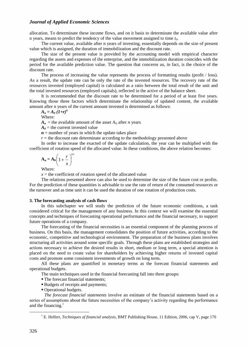
= The net treasury of exploitation activity 7 462,50 17 250,00

B. Investment activity

Payments for the equipments acquisition 0,00 -6 562,50

Payments for the patents acquisitions 0,00 -750,00

Receipts from the equipments sales 2 062,50 0,00

= The net treasury of investments activity 2 062,50 -7 312,50

C. The financing activity

The rambursation of the effects for payments -5 625,00 -5 625,00

Contractual debts rambursation -10 875,00 -1 875,00

Receipts from the options exercitation 937,50 0,00

Dividends payments 0,00 -1 500,00

= The net treasury from the financing activity -15 562,50 -9 000,00

D. The net treasury -6 037,50 937,50

Cash at the beginning of the period 5 437,50 -600,00

Cash at the end of the period -600,00 337,50

Minimum balance of cash 4 687,50 4 687,50

Necessary for financing at 31.12 5 287,50 4 350,00


333

Figure 1.3. The forecast of the net treasury at 31.12.2010

Statement of cash flow forecasting helps to highlight the movements of capital involved in the

balance sheet changes. Forward planning is limited to the static nature of the balance sheet showing

only financed deficit or surplus at a given moment of time, not the creation or variation of these funds.

3.4. The treasury budget

Known as the detailed projections of the cash flows, the treasury budgets are monthly or even

weekly planning vehicles, made in the financial department. The exclusive role of these budgets is to

plan receipts and payments over a period of time. The draw up of the receipts and payments budget

involves the continuous observation of the changes in the cash account in order to establish a level of

cash that would be sufficient to allow payments for falling due obligations. The financial analyst

should plan treasury activity in detail, showing exactly when the moment of cash inflows and

outflows.

The treasury budget shows any shortfall or surplus of funds. The treasury budgeting is a simple

process, much like personal budgeting of revenues and expenditures, where bills are paid with

proceeds from wages, rents, dividends, interest, etc. This correlation is necessary in order to align the

necessary of funds with the available cash. If the collection rate of the company debts from sales,

tends to decrease, there may be serious gaps in cash, as salaries and purchases must be paid currently.

Also, the unplanned payments for certain investments may create temporary needs that must be

covered. Given the emphasis on the level of detail of items, the treasury budget is the most

comprehensive expression of the cash flows analysis, because ultimately, all movements of funds are

included as changes in cash levels.

In order to draw up the treasury budget, must be detailed a plan of projected receipts and

payments. This plan reflects the net effect of the planned activity on the level of cash distributions,

except of the nature of depreciation, which doesn’t represent cash movements.

The time intervals covered by these budgets are selected according to the nature of the business

and trading conditions in which it operates. If the daily changes are significant, such as banks, daily

17 250,00

1 1 1

-7 312,50 -9 000,00

937,50

-10 000,00

-5 000,00

0,00

5 000,00

10 000,00

15 000,00

20 000,00

The forecast of the net treasury

Net treasury

Net treasury of the

financing activity

The net treasury of the Investment activity

The net treasury of the

operating activity


334

forecasts of these movements are necessary. In other circumstances there are sufficient weekly,

monthly or quarterly projections.

In the case of Alexandra SA we will create a treasury budget for the fourth quarter of 2009,

which will increase the capacity of understanding the cash flows of the company.

In the projected balance sheet are presented some basic data related to the business activity,

regarding the sales, production and acquisition. Also, we will present how the annual totals correlate.

For 2010 the totals presented were obtained similarly.

We considered useful to come up with a temporal scale, Table 1.1, in which we point out the

monthly sales volume. Using this scale, any forecast collection can be simulated by delaying cash

earnings by actual number of days of lag. A complete sales and collections plan of the receivables, at

30 days, looks like this:

Table 1.1.

Month

January February March April May June

Sales 15.000 25.000 30.000 45.000 40.000 42.000

Receipts 10.000 15.000 25.000 30.000 45.000 40.000

Figure 1.4. Sales forecasting

The forecasting of sales

15 000

25 000

30 000

45 000

40 000 42 000

0

5 000

10 000

15 000

20 000

25 000

30 000

35 000

40 000

45 000

50 000

1 2 3 4 5 6

Sales


335

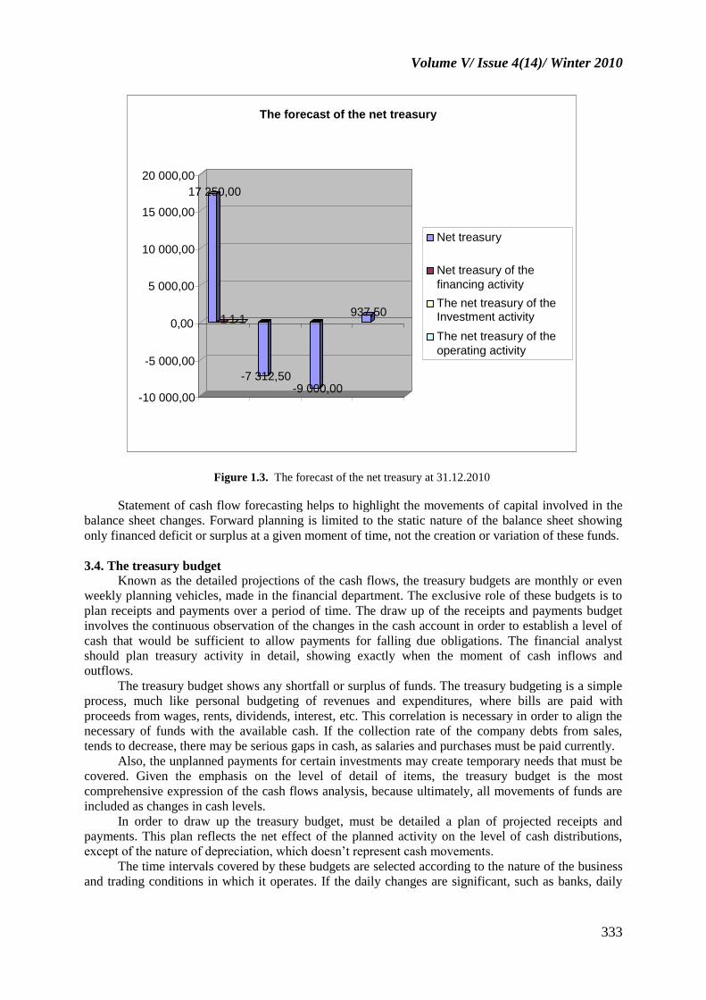
Figure 1.5. The forecasting of receipts

In the case of Alexandra SA Company, the recipients from the exercise of stock options and the

sale of equipments were budgeted in the months in which these transactions took place. The total cash

receipt for each month shows a trend of a lesser reduction than the monthly sales reduction. This

gradual reduction of debt collection is mitigated to a certain extent by the inoperative receipts from

issue of shares and sale of equipments.

If we analyze the cash utilization, we see a gap in terms of purchases on credit. In normal

conditions of a commercial loan for 45 days, we can consider that the parties made by the company

will be mistress for 45 days. Thus, the purchases made during the second half of August and in

September will be paid in October, a structure which will repeat for November and December.

For the fourth quarter of 2009 is provided a seasonal minimum, due to a reduction in sales and

operations since December, thus the period of immobilization of debts changes fast, in conditions of

higher cash receipts over a period of activity less intense than that provided for the reduction of

payments related to purchases and salaries. As a result of this situation, there is a net release of

operational capital, but they are not enough to offset the debt repayments scheduled for October and

November, only in December there is a certain balance between receipts and payments.

Against a possible increase in the volume of operational activity, it would have been necessary a

greater allocation of cash in the financing of the current assets, and thus requires an additional funding.

It can be observed this effect on projected statements for 2010, when the working capital is expected

to increase enough to offset the seasonal decline of the last quarter. If in the fourth quarter of 2009 was

also a period of growth, the treasury budget should have reflected the effect of lag in lower activities

of the previous months and the necessary of cash to finance the achieved production. It is clear that we

need a treasury budget drawn up very carefully, regardless of the business, as the operational level of

receipts and payments trend to fluctuate significant.

The payments related to the productive activity are based on the regressive pattern of production

and reflects a gradual reduction of the volume of inventories.

In order to make simple forecasts, the cost of sold goods was determined based on the sales

estimates. Thus, between the projected situation of the profit and loss account and the treasury budget

there may be some differences due to the different taxes on sales and production. To ensure

consistency is required to canvass the production structure, it must be estimated on the same basis of

The forecasting of receipts

0

5 000

10 000

15 000

20 000

25 000

30 000

35 000

40 000

45 000

50 000

1 2 3 4 5 6

Receipts


336

the sales. Such a difference can occur when minimum seasonal is used by the management to obtain

stocks in advance in order to increase the anticipated sales growth. The recognition of such differences

in sales and production structure represents a key for the increasing of the accuracy of performances

projection, achieving in the same time a correlation between the budgeting of the treasury results and

the projected financial statements.

The final result of the treasury budgeting represents the general picture of the effect of cash on

operational plans that they are based, establishing the cash needs or the surplus at the end of each

month. Note that, in our case, the excess cash at the end of 2009 (5.287.500 lei) and December 31,

2010 (4.350.000 lei) is identical to that obtained in the forecast financial statements. This is not

surprising, because we used the same assumptions throughout the preparation of forecasts.


337

Table 1.2. The projected treasury budget

- Thousand Lei - Luna Total trim. IV

2009

Total year

2010 August September October November December

Basic information

* Sold units 180.000,00 172.500,00 157.500,00 135.000,00 123.750,00 416.250,00 2.062.500,00

* Produced units 187.500,00 187.500,00 131.250,00 127.500,00 116.225,00 375.000,00 2.100.000,00

* Stocks changes 7.500,00 15.000,00 -26.250,00 -7.500,00 -7.500,00 -41.250,00 37.500,00

* Sales on credit 16.687,50 15.937,50 14.437,50 12.562,50 11.437,50 384.375,00 195.937,50

*Acquisitions on credit 2.850,00 2.775,00 1.950,00 1.875,00 1.725,00 5.550,00 31.500,00

Receivables

Claims collection 15.937,50 14.437,50 12.562,50 42.937,50 195.375,00

Options receipts 0,00 937,50 0,00 937,50 0,00

Receipts from equipments sales 0,00 0,00 2.062,50 2.062,50 0,00

TOTAL RECEIPTS 15.937,50 15.375,00 14.625,00 45.937,50 195.375,00

Payments - - - - -

Payments for acquisition 2.812,50 2.362,50 1.912,50 7.087,50 31.125,00

Salaries 2.100,00 2.093,75 1.875,00 6.018,75 33.937,50

Expenses for production 4.743,75 4.725,00 4.631,25 14.100,00 81.375,00

Marketing expenses 1.312,50 1.293,75 1.256,25 3.862,50 18.000,00

General expenses 750,00 750,00 750,00 2.250,00 8.812,50

Interests 0,00 0,00 656,25 656,25 3.187,50

Credit reimbursement 5.625,00 0,00 0,00 5.675,00 5.625,00

Tax payments 1.500,00 0,00 0,00 1.500,00 3.187,50

Contractual payments 0,00 7.500,00 3.375,00 10.875,00 1.875,00

Equipments acquisitions 0,00 0,00 0,00 0,00 6.562,50

Other assets acquisitions 0,00 0,00 0,00 0,00 750,00

Dividends 0,00 0,00 0,00 0,00 1.500,00

TOTAL PAYMENTS 18.843,75 18.675,00 14.456,25 51.975,00 194.437,50

NET RECEIPTS / PAYMENTS -2.906,25 -3.300,00 168,75 -6.037,50 937,50

Cumulated cash flow -2.906,25 -6.243,75 6.037,50 - -

The cash necessary analysis - - - - -

Initial cash 5.437,50 2.531,25 768,75 5.437,50 -600,00

Net receipts -2.906,25 -3.300,00 168,75 -6.037,50 937,50

Final cash 2.531,25 -768,75 -600,00 -600,00 337,50

Minimum balance of cash 4.687,50 -4.687,50 4.687,50 4.687,50 4.687,50

Total cash necessary 2.156,25 5.456,25 5.287,50 5.287,50 4.350,00


338

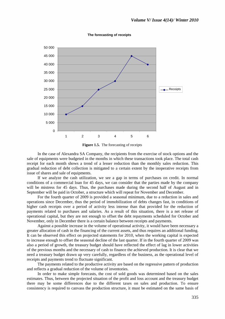
Figure 1.6. The projection of the cash necessary

In conclusion, the treasury budget shows under the form of specific details, the exact incidence

of receipts and cash payments. The treasury budget does not allow finding the minimum or maximum

available and to planning additional financial of the reimbursements, according to the existing needs.

Unlike the forecast situation, the forecast budgets may be prepared for each desired intervals within

the simulation period of fluctuations in cash flow.

If is based on the same assumptions regarding the production, sales volume and handling of

receipts, payments and trade credit, the treasury budget and the forecast situations will be similar

regarding the situations in the alert level of deficit or surplus funds at the end of the period for which

they are prepared.

3.5. Correlation between the company's financial forecast

Between the three typed of predictions (forecast financial statements, treasury budget and

operating budgets), presented in this subchapter, there is a close connection. Thus, they are based on

the same set of assumptions about returns and payments, repayment schedules, operating rates,

inventory levels, etc., these estimates may be correlated with each other precisely as in Figure 1.7.

If it starts from different assumptions about the vectors of influence used, particularly in the

forecast of the financial statements and treasury budget, then the financial plans and the deficit or

surplus funds will be different. Only through careful reasoning on key assumptions can be achieved

reconciliation between them, thus defining formats that contain sufficient detail and historical data

properly grounded.

The total cash necessary

0,00

1 000,00

2 000,00

3 000,00

4 000,00

5 000,00

6 000,00

1 2 3 4 5 6 7

August 2009

September 2009

October 2009

November 2009

December 2009

Trim. IV 2009

Total year 2010


339

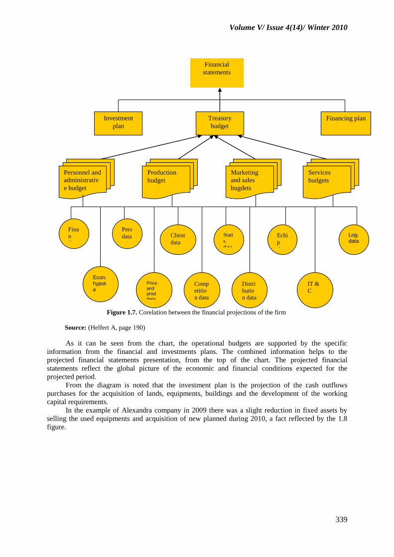
Figure 1.7. Corelation between the financial projections of the firm

Source: (Helfert A, page 190)

As it can be seen from the chart, the operational budgets are supported by the specific

information from the financial and investments plans. The combined information helps to the

projected financial statements presentation, from the top of the chart. The projected financial

statements reflect the global picture of the economic and financial conditions expected for the

projected period.

From the diagram is noted that the investment plan is the projection of the cash outflows

purchases for the acquisition of lands, equipments, buildings and the development of the working

capital requirements.

In the example of Alexandra company in 2009 there was a slight reduction in fixed assets by

selling the used equipments and acquisition of new planned during 2010, a fact reflected by the 1.8

figure.

Financial

statements

Investment

plan

Financing plan Treasury

budget

Personnel and

administrativ

e budget

Production

budget

Marketing

and sales

bugdets

Services

budgets

Fina

n

data

Pers

data

Econ. hypote

Client

data

Stati

s.

data

Echi

p

data

Log. data

Distri

butio

n data

IT &

C

Comp

etitio

n data

Price and prod data


340

Figure 1.8. The evolution of the fixed assets

It was also realized the construction of new manufacturing halls, located in its final stage of

completion, as is clear from the amount due and payable manufacturer (10.875.000 lei), reflected in

the balance of 31/09/2009 and is funded largely of long term debts contracted previously.

Taking into consideration the size of investments and production facility, the company may aim

to attract new long-term financing, whereas the estimates we have done in future operations indicates a

cash deficit on long term, necessary for the obligations payments in amount of 1.875.000 lei (see the

situation from the projected balance sheet).

The financing plan includes the schedule of future increases or decreases in debts or equity

during the projected period, which would involve a significant expansion or restructuring of the

company’s permanent capital, depending on capital requirements. Alexandra SA Company did not

plan any future funding but will require resources to cover the funding needs for the foreseeable future

(fourth quarter 2010), to avoid the dilution of the current monetary funds as the construction is

completed and paid.

In Figure 1.7, in addition to operational budgets and financial forecasts are presented a selection

of the essential information and their sources, information derived from the key and financial vectors.

In the case of Alexandra firm we used only the information provided by the management, which based

their estimates on the understanding of all the conditions affecting the business activity.

Any financial estimates involves both examining past trends as well as specific assumptions

concerning the future of key indicators of conditions that affect revenues, costs and other items of

receipts and payments.

The mathematical calculations, statistical methods and easy access to electronic databases

should not replace the human effort to make realistic assumptions regarding the national or global

outlook on the business performance, which may affect the company's expected performance. Also,

we must not forget that the past is just history; it is considered just the starting point in the forecast.

4. The calculation and covering of the treasury balances

To meet the forecast deficit balance, before resorting to loans are required to be taken the

following measures:

0,00

10 000,00

20 000,00

30 000,00

40 000,00

50 000,00

60 000,00

70 000,00

1 2

The net fixed assets




341

To act to advance the revenues cashing (by reducing the volume and/or duration of the trade

credits to customers or to request the casing in advance of sale’s incomes) and by delaying the

payments (the credit extension for suppliers in legal terms)

Trying to renounce for moment at some expenditures (investment, dividends, etc.).

Trying to achieve some exceptional revenues (sale of fixed assets etc.)

The deficit balance which is resulting from these measures is going be covered with new loans

and discount treasury, whose selection regards the treasurer ability to optimize the size of their actual

cost.

In order to realize a surplus of treasury positions is necessary an analysis of the origin of this

balance.It can come either from a higher working capital, due to contraction of financial debts without

immediate use or needed or a working capital too low, given the maturity of payments greater than the

revenues. In the first case the question of choosing between the cost of financial debt (long term) and

short-term investments, although in principle these two operations are not compatible (circulating

assets can not be covered in long-term loans). In the second case we can see a profitable cash

investment, with the smallest risk and the best liquidity.

In order to maximize the monetary surplus we can be made the following cash investments:

Negotiable monetary investments (investment contracts are not sold through input,

endorsement or negotiation on the stock exchange) term deposits, cash receipts, repurchase operations

etc.

Financial investments: stocks, bonds, options, etc.

In principle, the longer the more profitable is the placement, less liquid but, unlike short-term

investments which are more liquid, but have a lower rate of return.

References

[1] Agrawal A., and Jayaraman, N. 1994. The Dividend Policies of All-equity firms: A Direct Test of

the Theory of Free Cash Flow Theory. Managerial Decision Making Economics 15: 139-148.

[2] Albouy, M., and Dumontier, P. 1985. Faute des-il verser dividends?. Revue Français manageable, January.

[3] Battle, P. 2009. Actionnaires, financiers dirigeants et managers. Historique et perspectives. Revue

Français manageable 35: 319-342.

[4] Bistriceanu, G.D., Adochitei, M.N., and Negrea, E. 2001. The finances of economic agents.

Economic Publishing House. Bucharest.

[5] Bogdan, A.M. 2008. The Evaluation of Final Results in Time. Journal of Applied Economic

Sciences VolumeII Issue2 (3) Summer.

[6] Brezeanu, P. 2006. The financial analysis. Meteor Press Publishing House. Bucharest.

[7] Brezeanu, P. 2003. The financial diagnosis. The financial analysis tools. Economic Publishing

House. Bucharest.

[8] Doval, E. 2009. Dominant logic in investments in knowledge decision-making. Revista

Metalurgica International no.4 (2010). http:/www.metalurgia.ro/Metalurgia_International_

special4_2010.pdf.

[9] Doval, E. 2009. Return on investments in marketing integrated communications within global

environment. Revista Metalurgica International no.4 (2010).

[10] Dragotă, V. 2005. Practical approaches in the finances of companies. IRECSON Publishing

House. Bucharest.

[11] Dragotă, V. 2003. Financial management vol I. Economic Publishing House. Bucharest.

[12] Ungureanu, L., and Matei, V. 2008. Advances in Decisions Analysis. Efficient Methods in

Finance. Journal of Applied Economic Sciences. Volume III. Issue 4 (6).

*** Collections magazines: Tribune economics, Finance, Credit and accounting, General accounting

and expert review, The accounting and audit expertise business.

http://www.metalurgia.ro/Metalurgia_International_%20special4_2010.pdf.

http://www.metalurgia.ro/Metalurgia_International_%20special4_2010.pdf.

THE FORECASTING AND DIAGNOSIS ANALYSIS OF CASH FLOWS. … · THE FORECASTING AND DIAGNOSIS ANALYSIS...

Documents

Transcript of THE FORECASTING AND DIAGNOSIS ANALYSIS OF CASH FLOWS. … · THE FORECASTING AND DIAGNOSIS ANALYSIS...