The Floor Area Ratio Gradient: New York City, 1890-2007

Jason Barr Department of Economics

Rutgers University, Newark jmbarr@rutgers.edu

Jeffrey P. Cohen

Economics, Finance, and Insurance Department

Barney School of Business University of Hartford

professorjeffrey@gmail.com

January 28, 2014

Abstract

An important measure of the capital- land ratio in urban areas is the Floor Area Ratio (FAR),

which gives a building’s total floor area divided by the plot size. Variations in the FAR across

cities remain an understudied measure of urban spatial structure. We examine how the FAR

varies across the five boroughs of New York City. In particular, we focus on the FAR gradient

over the 20th century. First we find that the gradient became steeper in the early part of the 20th

century, but then flattened in the 1930s, and has remained relatively constant since the mid-

1940s. Next we identify the slope of the gradient across space, using the Empire State Building

as our core location. We find significant variation of the slope coefficients, using both ordinary

least squares and geographically weighted regressions. We then identify subcenters, and show

that while accounting for them can better capture New York’s spatial structure, by and large the

city remains monocentric with respect to its FAR. Lastly, we find a nonlinear and nonmontonic

relationship between plot sizes and the FAR across the city.

Key Words: New York City, floor area ratio, locally weighted regression JEL Classification: C14, R14, R33

2

1. Introduction

There is a large literature in economics on measuring the nature of urban spatial structure. The

focus of these works tends to concentrate on density or price measures relative to the urban

core.1 Collectively, this work has provided several key findings about the urban landscape. First,

the price and density gradients drop off at an exponential rate moving away from the center.

Second, over the 20th century there has been a steady and persistent flattening of the gradient, as

central cities have, to some degree, ―hollowed out,‖ while suburban districts have seen large

population and employment increases. Third, especially since the mid-20th century, urban spatial

structure has become poly-centric. With the rise of ―edge cities‖ and smaller suburban

agglomerations, population gradients -- while still dropping rapidly from the center -- tend to be

―bumpy‖ across space.

The aim of this work is to explore an important, but understudied, form of urban density—the

intensity of land use that comes from the buildings themselves; that is, the structural density of

the city (Brueckner, 1987). In particular we focus on the density of commercial structures. The

few studies on structural density have tended to focus on housing (McMillen, 2006), but much

less work has explored the ―shape‖ of commercial buildings across space and over time.

One important measure of structural density is the floor area ratio (FAR), which is the ratio of

total usable floor space to the size of the plot. For example, a 10-story building constructed on

the entire lot would have a FAR of 10, as would a 20-story building on half the lot. The FAR is

also a useful indicator of the capital- land ratio (McMillen, 2006, Clapp, 1980). As land values

rise closer to the city center where transport costs are lower, the monocentric city model implies

firms would substitute more capital (structure) for land (O’Sullivan, 2010).

As McMillen (2006) stresses, the monocentric model is static in nature. It details how density

should fall with distance from the center, at a given time, on the assumption that the parameter

values are fixed. To address this issue we investigate the density gradient over both time and

space. However, it might be the case that density and building age are related. If it is the case, for

example, that older structures tend to exhibit a steeper FAR gradient with respect to the center,

then not accounting for the age of the structure might bias the effects of distance from the center.

Thus if age and distance are positively correlated, omission of the age variable will tend to bias

the distance coefficients downward (or closer to zero). In this paper we control for possible

vintage effects by including in the regression the years of completion for each building.

In particular we focus on New York City from 1890 to 2009, and look at the FAR gradient

across the city. Using a data set over such a long period allows us to investigate the shape of the

gradient over time. Second, we investigate the degree to which the city is monocentric or not. As

1 Anas, et al. (1998) summarize the findings on the population density gradient. Work on land prices include

McMillen 1996 for Chicago and Atack and Margo (1998) for 19th

century New York. McMillen and Singell (1992)

provide evidence for wage grad ients.

3

we discuss in more detail below, we use the location of the Empire State Building as the center

of the city. New York City is comprised of 469 square miles of land, and contains a population

of 8.2 million people. Because it is so large, it can be considered a metropolitan region worthy of

investigation unto itself. Despite New York’s importance, its land use patterns remain

understudied.

In this paper we ask: (1) What does the structural density gradient look like relative to the

center? (2) Has it changed appreciably over time? (3) Is there evidence of poly-centricity within

the city itself? (4) Does controlling for the building age affect the estimates of the FAR gradient?

Since we have data on the plot size, we also examine how lot size affects structural density

across the city, investigating if lot size has a uniform effect, then is its effect is positive or

negative? On one hand a large lot size can promote structural density, since it allows for a more

efficient building layout and helps avoid the ―elevator problem‖ with skyscrapers, which must

allocate a large fraction of internal space for elevator shafts. But this may apply only where land

values are high. In areas were land values are lower, a large plot may encourage less density

because of a concave relationship between price per square foot and size (Colwell and Munneke,

1997). In other words, if the marginal cost of land is decreasing, so will the marginal provision of

structure. It remains an empirical question how plot size and structure density are related.

To answer these questions, we employ the methods of locally weighted regression. By and large,

the density gradient literature has assumed a constant gradient coefficient across space, and uses

ordinary least squares (OLS) to estimate the size of this coefficient. This assumption, however,

can lead to biased estimates or standard errors since gradients can change over both time and

space (McMillen and Redfearn, 2010). While OLS, for example, can include time dummy

variables, they are not able to capture the subtle movements of the gradient.

The LWR procedure estimates a separate coefficient for each observation. In particular, we

estimate geographically weighted regressions, which are based on the geographic distances of

each building from the others.2 We also incorporate a time dimension into the weight matrix that

links all the buildings together. Since our data set includes buildings completed over the 20 th

century, buildings completed in a certain year can only be influenced by completions in the same

or prior years.

LWR models are a more general approach that nests OLS. If the OLS assumption about constant

gradient coefficients is correct, then LWR and OLS will yield the same results. However, for

New York City, we find there is and has been a significant amount of variation in the FAR

gradient coefficients over both time and space, which demonstrates that the OLS assumptions do

not apply in this situation.

2In particular we use one specific form of Locally Weighted Regressions, namely Geographic Weighted

Regressions, which sets the weights as a function of the Euclidean distance between two buildings. For the

remainder o f the paper we the use the term LW R when referring the method used in this paper.

4

Based on our results, we find that the gradient for the city as a whole dropped over the first half

of the 20th century, then remained relatively steady between the late-1940s and mid-1980s, and

then dropped to a new plateau over the last quarter century. The evidence also suggests a further

flattening of the gradient since 2005.

On first approximation the monocentric model appears to be a good representation of structural

density in the city, but LWRs reveal several different ―centers of gravity,‖ which vary across

boroughs. For example, the Empire State Building is a useful ―center‖ for structures completed

within about 8 miles. After that, however, the further away one moves from the center, the less

likely its influence is on the density gradient. In particular we find positive gradient coefficients

at several points outside the center of the city. This provides evidence of several smaller ―nodes‖

within the city or adjacent to it. In addition we find that the exclusion of the year of completion

variable does not appreciably affect the distance coefficients, suggesting we need not be overly

concerned with vintage effects.

As another test for spatial structure, we first run an OLS regression of the log of the FAR on

several control variables, including the distance from the Empire State Building. Based on the

OLS residuals we then identity five areas in the city with clusters of large positive residuals. We

then include these ―subcenters‖ in the regressions and find that while distance to subcenter and

airports are statistically significant, they do not increase the R2 by very much; this suggests that

New York remains largely monocentric. Finally we investigate the LWR coefficients of plot size

on the FAR relative to the center. We find that closer to the core, the effect is positive, and that

after about four miles away from the center the effect becomes negative, on average, and after 10

miles virtually all the coefficients are negative. Further, since the functional form is non- linear, it

suggests that using OLS to estimate its affects may not be appropriate.

The rest of the paper is as follows. The next section provides a brief literature review. Then

Section 3 discusses the data and the results from ordinary least squares. Section 4 discusses the

results from the geographically weighted regressions. Section 5 discusses how we identify

subcenters and the results of OLS regressions with the subcenters. Section 6 presents the

estimated plot size coefficients on the FAR across the city. Finally, Section 7 provides some

concluding remarks.

2. Literature Review

There is a large literature on land rent and population gradients (Anas, et al., 1998), but little

known work that directly addresses the FAR gradient. Some works have contributed to the FAR

gradient literature indirectly, by examining the intra-urban location of tall buildings. One of these

is Frankel (2007), who studies the determinants of locations of tall buildings in the Tel-Aviv

municipal region. He finds, for example, a rising probability that 25+ floor buildings will

constructed in the core district; and the likelihood of these very tall buildings falls as one moves

away from the center. Clapp (1980) looks at the determinants of office space in the Los Angeles

5

metropolitan region, by estimating hedonic office rent equations. He finds that while subcenter

access and distance to employees are important factors, they are weak relative to the pull of the

central business district, where the benefits of face-to-face contacts remain strong.

For New York City, Atack and Margo (1998) investigate land value gradients during the 19 th

century, and find a general flattening of the land price gradient after the Civil War. Haughwout

et al. (2008) investigate the land value gradient from 1999 to 2006 in the New York City

metropolitan area; their aim is to create a land value index over the period. However, their data

show a substantial amount of land value variation in Manhattan, which suggests a standard

gradient model is too simple

McMillen (2006) is the only known work that directly addresses the FAR gradient. This research

includes estimation of the FAR gradient for individual homes in the city of Chicago, based on

both OLS and Spline function approaches. McMillen (2006) notes that closer to the core, lower

commuting costs should raise the value of land, which then should cause the FAR to be higher.

This is a crucial reason for studying the FAR gradient – that is, to confirm this common

underpinning of urban economics. If one confirms that the FAR gradient is downward sloping

and monotonic in a city with only one core, this is consistent with the monocentric city model

(O’Sullivan, 2010). One of our aims in this paper is to demonstrate that the FAR gradient for

Manhattan implies a variation of the monocentric city model with perhaps two cores – the

Empire State Building, and lower Manhattan–is applicable to the city. Furthermore, we

demonstrate that several of the boroughs of New York City have cores of their own, implying a

somewhat more intricate model than the simple monocentric city model might imply for a

smaller city.

As McMillen and Redfearn (2010) discuss, the use of OLS to measure effects that vary across

geographic space can lead to biased results. One can include both spatial and time related fixed

effects in the FAR gradient equation but these coefficients cannot capture the complex nature of

a spatial structure. Thus it is necessary to employ more spatially-oriented estimation procedures.

In particular, locally weighted regressions (LWR), by generating separate coefficient estimates

for each observation, allow for a much more nuanced measurement of an urban area’s spatial

patterns. Specifically, McMillen and Redfearn (2010) demonstrate that LWR leads to a much

smoother distribution of residuals than fixed effects estimation, as well as helps to mitigate

against omitted variable bias.

McMillen (1996) uses LWR to analyze land values in Chicago. His results show how the spatial

distribution of land values evolved from the 1830s to the 1990s. In the earliest period of

Chicago’s history, land values were generally rising uniformly approaching the city center.

However, LWR estimation shows that by the early twentieth century, land values took on a much

more diverse picture, with multiple and smaller peaks throughout the city. By 1990 the land

value gradients were quite varied throughout the city. A standard OLS approach would have

difficulty in capturing this complex pattern.

6

Meese and Wallace (1991) estimate hedonic housing price models with LWR to compare to

standard OLS estimates in several municipalities in California. By using LWR they can see how

index values are determined, once freed from the functional form restrictions of OLS. They find

that the LWR-generated indexes offer both considerable flexibility and precision. McMillen and

Redfearn (2010) estimate hedonic price functions in Chicago using LWR. Their results show that

the effect of distance to an elevated subway line in Chicago can have either a positive or negative

effect on housing price in different neighborhoods.

3. Data

The data set comes from the 2012 ―PLUTO‖ file provided by the New York Department of City

Planning (http://www.nyc.gov/html/dcp/html/bytes/dwn_pluto_mappluto.shtml, 2013). This file

lists extensive information for every property in the City of New York, including a unique

identification number (the ―BBL‖—borough, block and lot number), building address, latitude

and longitude coordinates, year completed, number of floors, the floor area ratio, the lot size, the

building type (and sub-type), and other information related to zoning, and land use.

For our analysis, we included observations from 1890 to 2009 which only had a single structure

on the property. In addition, we removed some properties that had some extreme outlier

characteristics, such as lots less than 100 square feet, and floor area ratios greater than 100. This

created a base data set with 662,161 total properties of all types. Of this we only investigate

commercial properties, i.e., those that housed a business of some kind.

The work on spatial structure aims to look at density changes relative to the central core. For this

paper, we chose the location of the Empire State Building (ESB), at West 34th Street and 5th

Avenue as the ―center.‖ We choose this location because the ESB is generally considered the

economic ―center of gravity‖ of the city (Haughwout, et al., 2009). It is in between lower

Manhattan and the high-rise office district between 42nd and 59th Streets. Manhattan, in

particular, in terms of its structural density is poly-centric.3 Because we are interested in the city

as a whole (which extends some 20 miles outward from the ESB), we use it as an approximate

center.

We also note that the Empire State Building was completed in 1931, and our data set includes

buildings from 1890 to 2009, so a large fraction of structures were completed before the ESB.

However, the ESB represents a kind of central base location, from which the gradient can be

calculated. Moving the center a mile or two in one direction does not appreciably affect the

conclusions. We also explore the issues of multiple centers in the paper as well.

3 See Barr and Tassier (2013) for the reason why midtown emerged as a separate business district.

7

3.1 Descriptive Statistics

Table 1 lists the different types of commercial properties in our sample. There are approximately

41,400 structures in our data set. Stores comprise the greatest proportion of commercial

structures, with a total of approximately 16,000 or 40 percent. Garages/gas stations, and offices,

are the next most common groups of commercial structures, with approximately 6,000 of each

type. The remaining types of properties include warehouses (approximately 5,200), factories

(approximately 3,600), and a relatively small number of lofts, hospitals, hotels, and theaters.

{Table 1: Distribution of Building Types across NYC}

Table 2 lists the distribution of structures across the five boroughs. Brooklyn (approximately 33 percent) and Queens (approximately 30 percent) have the greatest amount, with Staten Island

(slightly under 7 percent) last. Manhattan (17 percent) and Bronx (13 percent) are in the middle.

{Table 2: Distribution of Commercial Structures in the Five Boroughs of NYC}

Table 3 provides descriptive statistics for the FAR. As expected due to its relatively high land

values compared with the other boroughs, Manhattan has the greatest average FAR (and the

greatest standard deviation). Also, as predicted by its relatively low land values, Staten Island

has the lowest structural density in the city.

{Table 3: Descriptive Statistics for FAR across the Five Boroughs of NYC }

3.2 The FAR Gradient

Figure 1 shows the scatter plot of the log of FAR versus distance from the Empire State

Building. On average the gradient is negative, as would be expected; thought it does not appear

to be linear, as there appears to be a general flattening of the gradient further from the core.

Except for the ―bump‖ for downtown Manhattan, there does not appear to be any obvious other

sub-centers or deviations from the negative slope, but we will return to this issue in more detail

in Section 5.

{Figure 1: Scatter plot of lnFAR vs Distance to ESB}

3.3 OLS Results

In this section we present evidence on the nature of the FAR gradient from OLS equations. Table

4 presents the results. We present four equations. Equation (1) is the distance gradient from a

simple OLS regression. It shows that on, average, the FAR decreases about 13% per mile.

Equation (2) is the gradient with quadratic and cubic terms. As the scatter plot shows, adding

these terms provides a better fit, in terms of capturing the ―shape‖ of the gradient.

{Table 4: OLS Results}

8

Equation (3) provides an additional set of controls. We add in the log of the plot size and log of

plot size squared, the year and the year squared, borough dummies, and building type dummies.

For this we included dummies for the sub-categories of building. For example, ―warehouses‖ are

further divided by the city into ―fireproof,‖ ―semi- fireproof,‖ ―frame, metal,‖ etc. (See Pluto Data

Dictionary for full list of types).

Equation (1) shows that the simple OLS regression is able to account for about 25% of the

variation in the FAR gradient across the city. Adding the squared and cubed terms—Equation

(2)—brings it up to 31%.

For the plot area, we see a negative relationship overall. For the Year variable there is a negative

relationship, but the quadratic terms show a leveling off over time. Finally, we can see

differences in average FAR levels across the city. As expected Manhattan has the greatest far

(Staten Island is the omitted borough); Brooklyn, the Bronx and Queens, have roughly similar

FAR values, on average, while Staten Island has the lowest structural density in the city.

Equation (4) is the same as equation (3) but with the addition of polynomial terms for the

distance variable. They add a marginally better fit. In general, the addition of controls reduces

the size of the gradient coefficient. The polynomial terms show monotonicity is preserved.

4. Locally Weighted Regressions

Here, we use a version of weighted least squares, as suggested by McMillen and McDonald

(2004). Implementation of the model gives an estimated parameter for each target observation

(i.e., building):

βi = (∑ wijXjX’j)-1(∑ wijXjYj) ,

where Xj is a vector of control variables including the constant and the distance to the core for

each observation except i; Yj the dependent variable (log of FAR) for all observations except i;

wij is the weight that building j is given for building i; and the summations given by ∑ are taken

over all buildings, j, and wii =0.

We use a Gaussian (standard normal) weighting function (kernel) given by

where dij is the Euclidian distance between building i and j (as measured in degrees latitude and

longitude). McMillen (2010) notes that the choice of the kernel has little effect on the results

since most kernel choices have rapid decay with distance. b>0 is the bandwidth parameter,

discussed more below.

9

If the year of completion of the target observation, building i, was after the other buildings in the

data set then the weight is a function of the geographic distance. If not, then the weight was set to

zero.4

The bandwidth parameter determines the ―variance‖ of the weights. A larger b means that,

ceteris paribus, observations further away will have large weight values. For the LWRs, the

bandwidth value was selected using the standard cross-validation (C-V) method. The C-V

algorithm runs a LWR for each observation for a specific bandwidth value. Then a statistic is

generated that is the mean squared residual of the LWR, where the residual is the difference

between the target value (i.e., lnFARi) and the predicted target value, after omitting the ith

observation from the model. The bandwidth that minimizes this statistic is used. See McMillen

and McDonald (1997) for more information.

For each estimated coefficient we also calculate a standard error, given by equation 2.21 in

Fotheringham et al. (2002). This approach is similar to the F-statistics calculations procedure

described in the appendix of McMillen and Redfearn (2010).

4.1 LWR Results

For the LWRs, we regressed the log of the floor area ratio ( lnFAR) on the log of plot size

(lnArea), the year the building was constructed (Year) and the distance to the Empire State

Building (DESB). Note that the results are from using a bandwidth that minimize the C-V,

which in this case gives b=0.02. We also compare the results from a regression of LnFAR on

DESB and LnFAR on DESB and lnArea, omitting the year.

Table 5 gives the descriptive statistics for the results. We separate the coefficient results into

each borough for comparison. First, focusing on the distance coefficients we see that, on average,

Manhattan has the largest (in absolute value) coefficients, and that the average and median are

negative.

4.2 FAR Gradient over Time

Figure 2 shows the averages of the coefficients for each year. Figure 2a shows the (unweighted)

averages of all the coefficients with standard errors bands equal +/-1.96*(average of the standard

errors). They show that starting in the 1920s, there was a general flattening of the gradient

across the city. Then between around 1940 and 1985 the gradient remained relatively constant,

hovering in the -0.11 range, when it started to flatten again. However, since the mid-2000, the

average has started to decline a bit.

Anas et al. (1998) report estimates for the population density gradient at three points in time (in

miles), 1900, 1940, and 1950. They find it to be 0.32, 0.21, and 0.18, respectively. McDonald

and McMillen (2007) report population a density gradient of 0.12 for New York in 2000. While

4 Setting some weights equal to zero is analogous to specifying a ―window‖ (see McMillen and Redfearn, 2010).

10

our results show the same direction, the FAR gradient for the city of New York appears to have

small coefficients (in absolute value). For the decade of 1900 to 1909 our coefficient averages

about 0.11, for the 1940s, the average is 0.05, 1950s is 0.06, and for 2000s is 0.04. Note that

some of the difference across studies might also be related to the size of regions. Here we focus

on only New York City, but when other studies include metropolitan areas it is likely to increase

the size of the gradient, if density falls off rapidly outside of the central city proper.

Figure 2b shows the averages of the coefficients over time for each borough separately. It shows

that there are different patterns between Manhattan and the outer boroughs over time (Staten

Island is omitted to increase clarity). By and large, the outer boroughs showed a general gradient

flattening between 1900 and 1940, and have remained relatively constant since then.

{Figure 2a and 2b: Avg. LWR coefficients over time.}

Manhattan, on the other hand, has shown a different pattern. First, the average coefficients have

consistently remained large (in absolute value) as would be expected given its importance in the

national economy and its higher land values. Second we see that an opposite trend as compared

to the other boroughs: the gradient in Manhattan appears to have steadily fallen until the early

1960s. From there, over time, the gradient has flattened out. The gradient coefficients also show

much more variation from year to year in Manhattan. In addition, Manhattan’s gradient seems

much more sensitive to the business cycle—falling in years in which the economy is growing,

and moving closer to zero in the years the economy is in recession or depression. For example,

the 1930s to early 1940s, shows the coefficients moving closer to zero, then dropping until the

mid-1960s. Another ―spike‖ toward zero occurs in the mid-1970s and the 1990s. The FAR’s

movements over the course of the business cycle suggests that land values are quite sensitive to

economic activity at the national level.

Figure 3 shows the coefficient estimates versus distance from the Empire State Building. The

results of each borough are presented in separate graphs. The overall pattern shows that the

coefficients very close the Empire State Building are quite large (in absolute value) and moving

away they get closer to zero. In general they flatten out, between mile 5 and 15. Then after that

there are two areas, one at mile 15 and one at mile 20 where the coefficients go above zero This

suggests that in these two areas there are smaller subcenters, on the fringes of the city. We have

more to say about the subcenters in section 5 below. Figure 3 suggests that OLS estimates are

misleading with regard to the shape of the coefficients across the city.

{Figure 3a-d: LWR coefficients vs distance from ESB by borough}

Figure 4 presents a type of intensity map for the distance coefficient estimates (Fotheringham,

2002). Each point on the map is a t-statistic equal to the coefficient estimate divided its standard

error. It shows the relative magnitude of the coefficients. Here we see concentric bands of

coefficients; with the regions of positive coefficients. The dark red dots show the largest t–stats

(in absolute value) and they are a semi-circular area around the Empire State Building.

11

The next semi-circle around that has smaller t-statistics, but all above 10 in absolute value. Two

clusters of black dots (positive t-statistics) occur in three locations (the one in south-western

corner of Staten Island is not shown on the map). One is located in Jamaica, Queens; the other is

Far Rockaway, Queens. These suggest local ―centers of gravity.‖ Jamaica is a local

transportation hub for the Long Island Railroad; Far Rockaway, perhaps, attracts business near

John F. Kennedy Airport. The third cluster is in south west Staten Island, across the river from

Perth Amboy, New Jersey (not shown on map).

{Figure 4: T-stats map for LWR Coefficients}

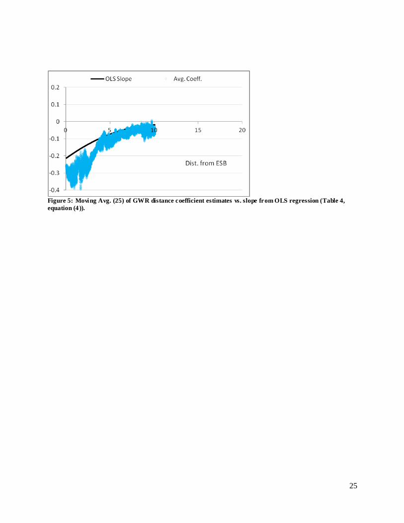
Since the LWR estimates give the slope of the density gradient, we compare them to the slope

coefficients from OLS. In particular, we first took a moving average (25) of the LWR

coefficients versus the distance to the ESB and plotted the scatter plot in Figure 5. Also

presented is the slope of the estimated coefficients from the OLS regression equation (4) Table 4.

In particular, we graph

∂lnFARHat/∂(DESB)=-.215+2(.019)DESB-3(0.001)DESB2.

Figure 5 shows the results. Over the graph suggests a kind of glass-half- full/glass-half-empty

results. On average, the OLS slope coefficients share similar movement compared with the LWR

coefficients; however, the LWR coefficients are able to capture more subtle movements in the

density landscape.

Finally, we reran the LWRs without the year to see if its omission dramatically changed the

distance to the ESB coefficients. We found that it did not. In fact, the correlation coefficient for

the two sets of coefficients was .99, and a regression of coefficients without the year on the

coefficients with year gave an estimated slope coefficient of 1.01 and p-value=0.00. This

suggests that LWRs might offer an ―antidote‖ to the problem of omitted variable bias.

5. Subcenter Identification

As a method to identify possible subcenters in New York City, we used the residuals from

equation (4), table 4. From this list of residuals we then mapped the clusters of residuals that (a)

were greater than 1.47 (two standard deviations away from 0), and had more than 15 of these

residuals within a quarter mile of each other. From this procedure we identified 6 centers or

subcenters in order of size (based on size of cluster). Figure 6 shows the results.

{Figure 6: Map of Subcenters}

In Manhattan the area is north of Grand Central Station (Park and 53rd Street) and Wall Street. In

Brooklyn, there is downtown Brooklyn , and in Queens there is Flushing and Jamaica, and in the

Bronx there is The Hub neighborhood (at East 149th and Third Avenue). The process did not

yield any centers for Staten Island. We note that technically midtown and downtown are not

12

subcenters, but actual centers in their own right, but for exposition we refer to them as subcenters

because of the way we identify them in this section.

A word is in order about the criteria we used. We recognize there is some arbitrariness in

determining the subcenters across the city. However, our aim is to find the largest and most

important ones. If we reduced either one of the thresholds, we risked the possibility of including

false positive identifications, in the sense that a cluster of positive residuals might simply reflect,

for example, a public housing development rather than a true concentration of structural density.

In the end the rule we chose seemed to be a reasonable balance between identifying subcenters

while not being overly liberal. The OLS regressions bear this out in the sense that the coefficient

estimates for the distance to subcenters are statistically significant, but even including the largest

ones don’t increase the R2 by a large amount. Also note that we obtained the exact same centers

when positive residuals greater than one standard deviation, and 45 or more were clustered

within a quarter mile of each other.

We also note that work by McMillen (2001) has used LWRs to identify subcenters. With our

data set, we found that we were able to identify the same subcenters when using the LWR

residuals. In particular, when we took positive LWR residuals that were one standard deviation

away and had 15 or more clustered within a quarter mile of each other, the same six subcenters

appeared.

Lastly, we also included measures of the distance to the closest airport. New York City has two

airports, Laguardia and John F. Kennedy. Distance to these might also affect density, since they

are transportation hubs. In the end, we found that the best specification was to divide the distance

variable into two. The first variable is the distance to the closest airport times a dummy variable

that takes on the value of one if the distance is less than five miles, and zero otherwise. The

second variable is the distance to the airport times a dummy variable that takes on the value of

one if the distance is between five and ten miles away, and zero otherwise. The results show that

moving further away the effect of the airports diminishes. For locations close the airport the FAR

density gradient is close to 0.06 on average. For the next group it falls to about 0.014, on

average.

6. The Effect of Plot Size Across the City

In both the OLS regressions and LWRs we included the plot size as an explanatory variable. The

OLS results show that, on average, there is a negative relationship between the lot size and the

FAR, though the functional form appears nonlinear. Figure 7 shows a scatter plot of the plot area

estimated coefficients versus the distance from the Empire State Building. Here we can see that

the LWRs paint a more subtle picture as compared to the OLS results. Each borough is given a

different color to see how the coefficients vary across the city.

13

The results show that for most of Manhattan and the western portions of Brooklyn and Queens,

the coefficient estimates are positive, on average. After about four miles away, the average

becomes negative, and slowly decreases, so that by 10 miles away virtua lly all of the coefficients

are less than zero. As well the magnitude of the coefficients (in absolute values) steadily

becomes larger as one moves away from the center.

While we leave a more detailed treatment of this result for future work, the relationship is most

likely due to three factors: land values, the types of businesses, and zoning. Because land values

are much higher closer to the center, each plot of land is likely to be used more intensively.

Having a larger plot of land allows the developer to overcome the problems associated with

elevators. Since a skyscraper requires that a large fraction of its internal space is devoted to

elevator shafts, a larger lot can allow a developer to build a taller building and reap a greater

return (Barr, 2012).

Moving away from the center, as land values drop, there is less economic pressure to use the plot

more intensively, and our results show that, in fact, at some point, larger plots are associated with

less structural density. This negative effect might also be related to the types of businesses that

are likely to locate further out from the center. In particular, in the outer boroughs there are more

likely to be retail services that cater to the neighborhood populations, including supermarkets,

shopping centers, and automobile repair shops. These types of stores mostly likely prefer a

flatter, rather than taller, configuration because it is easier for shoppers or workers to navigate

through the space.5

Lastly, it is also likely that zoning rules play a role. First if the zoning laws reduce the FAR

limits in the suburban parts of the city, it will legally promote the relationship we see in Figure 7.

Second, if the zoning rules require developers to provide on-site parking, then this will force a

less- intensive use of space, all else equal. Where land values are relatively cheap, developers

prefer to provide grade-parking, rather than decks or underground garages, because of the

additional expense.

Conclusion

This paper explores a less commonly investigated component of urban spatial structure—the

Floor Area Ratio (FAR), which is a measure of the capital- land ratio. In particular, our goal is to

investigate the FAR gradient across both time and space. We focus on New York City from 1890

to 2009, incorporating practically every extant commercial building in the city—some 40,000

structures completed over the last 120 years. By controlling for the age of the structures, we are

able to determine the FAR gradient over time, with little concern for possible vintage effects.

5 Consider that even in Manhattan most supermarkets are on one floor, and occasionally, only in the most busy

districts do you sometimes find a supermarket with a second level.

14

We estimate the FAR gradient by both ordinary least squares (OLS) and locally weighted

regressions (LWRs). We find that the LWRs are better able to better capture the changes in the

gradient over time, as compared to OLS. In particular we find that the gradient steepened in the

early part of the 20th century, and then began to flatten in the mid part of century, with a plateau

around 1945.

We also find a very different gradient pattern over time in Manhattan, relative to the other

boroughs. In particular, Manhattan’s FAR gradient is much steeper, as would be expected, but it

also appears to be very sensitive to the business cycle—flattening during downturns and

becoming steeper during boom times. This most likely reflects the sensitivity of Manhattan’s

land values to the general level of U.S. output.

Next we compare the LWR gradient coefficients to the slope of the OLS coefficients. We find

that while a cubic functional form for OLS is a reasonable measure of the FAR gradient, it does

not capture the more subtle patterns across space. In particular we find that in some locations in

the outer boroughs the gradient with respect to the center is positive.

This suggests then that there are other ―centers of gravity‖ throughout the city. To explore this in

more detail we identify possible subcenters by looking at positive clusters of OLS residuals. This

procedure identifies six subcenters (two in Manhattan, one in Brooklyn, one in the Bronx and

two in Queens). We then rerun the OLS equations with distance to nearest subcenter and distance

measures to the city’s airports. We find that while these additional controls are statistically

significant, they do not appreciably increase the R2, suggesting that beyond Manhattan,

subcenters are not as important.

Finally, we investigate the relationship between the plot area coefficients from the LWRs and

distance from the center. We find that close to the center, the coefficients are positive, suggesting

that large plots allow land to be used more intensively there. But moving away from the center

the relationship becomes negative, on average, suggesting large plots are used less intensively

further away from the center. We leave further exploration of this relationship for future work,

but we hypothesize that it is related to land values, the mix of businesses in different parts of the

city, and zoning regulations.

15

References

Anas, A., R. Arnott., and K.A. Small. 1998.―Urban spatial structure.‖Journal of Economic Literature, 36(3), 1426-1464.

Atack, J., and Margo, R. A. 1998. ―Location, Location, Location!‖ The Price Gradient for

Vacant Urban Land: New York, 1835 to 1900. The Journal of Real Estate Finance and

Economics, 16(2), 151-172.

Barr, J. 2012. ―Skyscraper Height.‖ The Journal of Real Estate Finance and Economics, 45(3), 723-753.

Brueckner, J. K. 1987. ―The Structure of Urban Equilibria: A Unified Treatment of the Muth-

Mills Model.‖ In Handbook of Regional and Urban Economics, Volume II. Ed. E.S. Mills.

Elsevier Science Publishers.

Clapp, J. M. 1980. ―The Intrametropolitan Location of Office Activities.‖ Journal of Regional Science, 20(3), 387-399.

Colwell, P. F. and Munneke, H. J. 1997. ―The Structure of Urban Land Prices.‖ Journal of

Urban Economics, 41(3), 321-336. Frankel, A. 1997. ―Spatial Distribution of High-rise Buildings within Urban Areas: The Case of

the Tel-Aviv Metropolitan Region.‖ Urban Studies, 44(10), 1973-1996.

Fotheringham, A. S., C. Brunsdon and M. Charlton. 2002. Geographically weighted regression :

the analysis of spatially varying relationships, Hoboken, NJ: Wiley.

Haughwout, A. Orr, J. and Bedoll, D. 2008. ―The Price of Land in the New York Metropolitan

Area.‖ Current Issues in Economics and Finance, 14(3),1-7.

McDonald, J. F. and D. P. McMillen. 2007. Urban Economics and Real Estate: Theory and Policy, Wiley.

McMillen, D. P. 1996. ―One Hundred Fifty Years of Land Values in Chicago: A Nonparametric

Approach.‖ Journal of Urban Economics, 40, 100-124. McMillen, D. P. 2001. ―Nonparametric Employment Subcenter Indentification.‖ Journal of

Urban Economics, 50, 448-742.

McMillen, D. P. 2006. ―Testing for Monocentricity.‖ In A Companion to Urban Economics, eds

R. J. Arnott and D. P. McMillen. Malden: Blackwell Publishing.

16

McMillen. D. P. 2010. ―Issues in Spatial Data Analysis.‖ Journal of Regional Science, 50(1), 119-141.

McMillen, D. P. and Redfearn, C. L. 2010. ―Estimation and Hypothesis Testing for

Nonparametric Hedonic House Prices Functions.‖ Journal of Regional Science, 50(3), 712-733. McMillen, D. P. and Singell, Jr. L. D. 1992. ―Work Location, Residence Location and the

Intraurban Wage Gradient. Journal of Urban Economics, 32(2), 195-213.

Meese, R. and Wallace, N. 1991. ―Nonparametric Estimation of Dynamic Hedonic Price Models and the Construction of Residential Housing Price Indices.‖ Real Estate Economics, 19(5), 308-332.

O'Sullivan, A., 2010. Urban Economics, 7th edition. McGraw-Hill.

17

Tables

Building Type Count Percent

Stores 16,726 40.4

Garages/Gas Stations 6,738 16.3

Offices 5,959 14.4

Warehouses 5,240 12.7

Factories/Industrial 3,644 8.8

Lofts 1,287 3.1

Hospitals/Health 987 2.4

Hotels 662 1.6

Theaters 154 0.4

Total 41,397 100

Table 1: Distribution of Building Types across NYC (excludes residential buildings, asylums and nursing

homes, houses of worship, condominiums, parks buildings, and utility properties)

Borough Frequency Percent Cumulative

Brooklyn 13,942 33.68 33.68

Bronx 5,407 13.06 46.74

Manhattan 6,857 16.56 63.3

Queens 12,447 30.07 93.37

Staten Island 2,744 6.63 100

Total 41,397 100

Table 2: Distribution of Commercial Structures in the Five Boroughs of NYC

Borough Mean Std. Dev Min. Max. Nobs.

BK 1.38 1.20 0.01 23.96 13,567

BX 1.13 0.94 0.01 12.14 5,132

MN 5.84 5.87 0.02 87.67 6,831

QN 1.20 1.37 0.01 37.6 11,781

SI 0.65 0.50 0.01 6.03 2,642

NYC 2.00 3.18 0.01 87.76 39,353

Table 3: Descriptive Statistics for FAR across the Five Boroughs of NYC *difference is nobs . are due to

missing FAR values .

18

(1) (2) (3) (4)

Dist. to Empire State -0.129 -0.507 -0.053 -0.215

(109.10)** (64.98)** (37.60)** (22.65)**

(Dist. to ESB)2 0.044 0.019

(42.67)** (16.87)**

(Dist. to ESB)3 -0.001 -0.001

(34.13)** (15.41)**

Ln(Lot Area) -0.168 -0.177

(3.14)** (3.32)**

Ln(LotArea)2

0.005 0.005

(1.48) (1.63)

Year -0.46 -0.477

(20.25)** (21.05)**

Year2 0.0001 0.0001

(20.22)** (21.02)**

Brooklyn Dummy 0.353 0.424

(20.06)** (22.48)**

Bronx Dummy 0.305 0.366

(16.16)** (18.00)**

Manhattan Dummy 1.27 1.163

(52.03)** (46.23)**

Queens Dummy 0.266 0.309

(15.14)** (16.84)**

Constant 1.05 1.79 452.1 468.9

(109.35)** (106.49)** (20.35)** (21.16)**

# Observations 39953 39953 39944 39944

R2 0.26 0.31 0.42 0.42

Building Type Dummies Yes Yes

P-val for Dummies 0.00 0.00

Table 4: OLS Regression Results. Dependent Variables is ln(FAR) for commercial structures. ** Stat. sig. at

99% ; *Stat. sig. at 95% . Absolute value of robust t-statistics below coefficient estimates.

19

Variable Mean St. Dev.

Avg. St.

Err. Min. Max. # Obs.

New York City

Dist. ESB -0.11 0.12 0.02 -1.27 1.77 39944

Ln(Area) -0.06 0.22 0.03 -1.68 1.30 39944

Year -0.01 0.03 0.01 -0.83 2.38 39944

Brooklyn

Dist. ESB -0.10 0.09 0.01 -0.55 0.35 13566

Ln(Area) -0.10 0.11 0.03 -1.03 1.30 13566

Year -0.01 0.01 0.00 -0.68 1.00 13566

Bronx

Dist. ESB -0.09 0.05 0.02 -0.80 0.76 5132

Ln(Area) -0.08 0.10 0.04 -1.19 0.62 5132

Year -0.01 0.02 0.00 -0.23 0.41 5132

Manhattan

Dist. ESB -0.23 0.13 0.02 -0.67 0.25 6829

Ln(Area) 0.32 0.15 0.03 -1.41 0.49 6829

Year 0.00 0.05 0.01 -0.10 2.38 6829

Queens

Dist. ESB -0.09 0.13 0.02 -1.27 1.77 11780

Ln(Area) -0.15 0.13 0.03 -1.68 0.73 11780

Year -0.01 0.02 0.01 -0.83 0.66 11780

Staten Island

Dist. ESB -0.08 0.13 0.04 -1.26 0.56 2637

Ln(Area) -0.32 0.11 0.06 -1.00 0.96 2637

Year 0.00 0.02 0.01 -0.59 0.40 2637

Table 5: Descriptive statistics for coefficient estimates from the locally weighted regressions.

20

(1) (2) (3) (4)

Dist. to Empire State Bldg. -0.215 -0.238 -0.203 -0.213

(22.86)** (18.71)** (21.34)** (16.76)**

(Dist. to ESB)2

0.019 0.026 0.017 0.022

(17.54)** (13.97)** (15.67)** (12.01)**

(Dist. to ESB)3

-0.001 -0.001 -0.0004 -0.001

(13.78)** (12.18)** (11.75)** (10.48)**

Ln(Area) -0.19 -0.14 -0.198 -0.145

(3.60)** (2.65)** (3.73)** (2.74)**

Ln(Area)2 0.006 0.003 0.006 0.003

(1.91) (1.00) (2.10)* (1.15)

Year -0.454 -0.453 -0.455 -0.452

(20.24)** (20.38)** (20.28)** (20.37)**

Year2

0.0001 0.0001 0.0001 0.0001

(20.21)** (20.34)** (20.25)** (20.33)**

Brooklyn Dummy 0.239 0.579 0.274 0.627

(11.50)** (21.75)** (12.42)** (22.83)**

Bronx Dummy 0.105 0.458 0.212 0.594

(4.40)** (15.64)** (8.41)** (19.44)**

Manhattan Dummy 0.872 1.193 0.93 1.27

(30.56)** (37.03)** (31.97)** (38.81)**

Queens Dummy 0.018 0.411 0.138 0.571

-0.78 (14.03)** (5.76)** (18.79)**

Dist. to Closest Subcenter -0.064 -0.211 -0.072 -0.237

(21.04)** (20.67)** (23.30)** (23.07)**

(Dist. to Subcenter)2

0.026 0.03

(12.76)** (14.51)**

(Dist. to Subcenter)3

-0.001 -0.001

(6.24)** (7.71)**

Dist. Closest Airport x Less than 5 Miles -0.057 -0.064

(16.35)** (18.31)**

Dist. Closest Airport x (5 – 10 Miles) -0.015 -0.013

(9.34)** (8.61)**

Constant 446.4 444.8 447.0 443.9

(20.37)** (20.50)** (20.42)** (20.50)**

R-squared 0.43 0.44 0.43 0.44

Table 6: OLS regressions with distance to closest subcenter and airport . Robust t-statistics in parentheses. **

Significant at 99% ; * significant at 95% . Note all regressions have 39,944 observations; all include building

types dummies (with p-values =0.00).

21

Figure 1: Scatter plot of ln(FAR) versus distance from the Empire State Building for Commercial Structures.

22

Figure 2. Top (2a): average LWR coefficients over time for NYC, 1900-2009. Bottom (2b): average

coefficients over time for each borough (Staten Island Not shown), 1910-2009.

23

Figure 3: LWR coefficient estimates vs. distance from the Empire State Building (miles). Top left (3a): Manhattan and Bronx. Top right (3b): Brooklyn.

Bottom left (3c): Queens. Bottom Right (3d): Staten Island. Note vertices may have different lengths across graphs.

24

Figure 4: Map of t-stats of GWR distance to ESB coefficients. Note Staten Island note shown.

25

Figure 5: Moving Avg. (25) of GWR distance coefficient estimates vs. slope from OLS regression (Table 4,

equation (4 )).

26

Figure 6: Clusters of positive residuals used to identify sub-centers in New York City.

27

Figure 7: Scatter plot of plot area coefficients from GWRs versus distance from the Empire State Building