GEOTECHNICAL ENGINEERING DIVISION FACULTY OF ENGINEERING

CAIRO UNIVERSITY

THIRD GEOTECHNICAL ENGINEERING CONFERENCE

CAIRO UNIVERSITY

JANUARY 5-8, 1997

THE FLAT DILATOMETERDESIGN APPLICATIONS

KEYNOTE LECTURE

Silvano Marchetti

L'Aquila University, Italy

-1-

THE FLAT DILATOMETER : DESIGN APPLICATIONS

Silvano Marchetti

Faculty of Engineering, L'Aquila University, Italy ABSTRACT Since the writer's 1980 ASCE paper (Marchetti, 1980), a considerable amount of literature has been published on the DMT interpretation and design applications. Scope of this report is to highlight a number of significant new findings and practical developments.

1. INTRODUCTION A detailed description of the DMT equipment and

of the initial correlations can be found in the 1980 ASCE paper and will not be repeated herein. Recommended comprehensive references are : Lunne et al. (1989), U.S. DOT (1992), Lutenegger (1988), ASTM Subcommittee D 18.02.10 (1986), Eurocode 7 (1995), Marchetti & Crapps (1981), Schmertmann (1988) (the latter reference, while highly informative and detailed, is bulky and unfortunately difficult to procure). This report tries to avoid material readily found elsewhere. However a brief review of the test methods and of the 1980 correlations is given. Then a number of significant new findings and practical developments are reviewed.

2. ORGANIZATION OF THIS REPORT To help the reader to find the topic of interest, the following table was prepared:

3. DESCRIPTION OF EQUIPMENT AND TEST PROCEDURE

4. INTERPRETATION IN TERMS OF SOIL PROPERTIES AND PARAMETERS 4.1 INTERMEDIATE PARAMETERS

4.2 CONSTRAINED MODULUS M (SAND AND CLAY)

4.3 MODULUS E' (SAND AND CLAY)

4.4 MAXIMUM SHEAR MODULUS GO

4.5 UNDRAINED SHEAR STRENGTH Cu

4.6 OVERCONSOLIDATION RATIO OCR

4.7 Ko IN SITU

4.8 FRICTION ANGLE φφ ' (SAND)

4.9 DR (SAND)

4.10 FLOW CHARACTERISTICS AND PORE PRESSURES

5. PRESENTATION OF DMT RESULTS

6. DISTORTIONS CAUSED BY THE PENETRATION

7. SPECIAL CONSIDERATIONS 7.1 SOME COMMENTS ON THE CURRENT

ROLE OF INSITU TESTING

7.2 PARAMETER DETERMINATION BY "TRIANGULATION"

7.3 DRAINAGE CONDITIONS DURING THE DILATOMETER TEST

8. APPLICATION TO ENGINEERING PROBLEMS 8.1 SETTLEMENTS OF SHALLOW

FOUNDATIONS 8.2 VERTICALLY LOADED PILES

8.3 LATERALLY LOADED PILES

8.4 LIQUEFACTION

8.5 DETECTING SLIP SURFACES IN OVERCONSOLIDATED CLAY SLOPES

8.6 MONITORING DENSIFICATION / STRESS INCREASE

8.7 MONITORING DENSIFICATION/ STRESS DECREASE

8.8 SUBGRADE COMPACTION CONTROL

9. CORRELATION WITH PARAMETERS OBTAINED BY OTHER IN SITU TESTS

10. DIFFERENCES VS AXISYMMETRIC PROBES 10.1 CONSEQUENCES OF PROBE ' S SHAPE.

ARCHING. 10.2 INCREASED COMPLEXITY OF THE

THEORETICAL MODELS

11. CONCLUDING REMARKS 11.1 GUIDE TO THE USE OF DMT IN THE

APPLICATIONS 11.2 PERCEIVED ADVANTAGES

12. BIBLIOGRAPHY

Third Geotechnical Engng. Conf. Cairo University, 421-448 (26 pp.) 5-8 Jan. 1997. Keynote lecture

-2-

3. DESCRIPTION OF EQUIPMENT AND TEST PROCEDURE

The dilatometer (Fig. 1) consists of a steel blade having a thin, expandable, circular steel membrane mounted on one face. The blade is connected, by an electro-pneumatic tube, running through the insertion rods, to a control unit on the surface. The test starts by inserting the dilatometer into the ground. By use of a control unit with a pressure regulator, a gauge and audio signals, the operator determines, in about 1 min, the po-pressure required to just begin to move the memb rane and the p1-pressure required to move

its center 1.1 mm into the soil. The blade is then advanced into the ground of one depth increment, typically 20 cm, using

Fig. 1. General layout of the Dilatometer Test common field equipment. The blade can be: − Pushed, with a Cone penetrometer rig. This method

yields the highest productivity, up to 100 m of profile per day

− Pushed, with the hydraulic capability of a drill rig

− Driven, with SPT or lighter equipment (hammer and rods).

In most cases a DMT sounding starts from the ground surface, with the tube running inside the rods. Alternately, one can start testing from the bottom of a borehole. In this case the tubing can either run all the way up inside the rods, or can exit laterally from the rods at any point above the blade. In all cases the penetration must occur in fresh (not previously penetrated) soil.

3.1.1.1 REMARKS ON THE WORKING PRINCIPLE − The membrane expansion is not a load controlled

test (apply the load and observe settlement) but a displacement controlled test (impose displacement and measure the required pressure). Thus in all soils the central displacement (and at least approximately the strain system imposed to the soil) is the same. It can be noted that the 1.1 mm displacement to 60 mm diameter is proportionally equivalent to a 1.1 m central settlement of a 60 m diameter storage tank.

− The membrane is not a measuring organ but a passive separator soil-gas. The measuring organ is the gage at ground surface. The accuracy is that of gage. The zero offset of the gage can be checked at any time, being at surface. The gage can be replaced with a lower scale gage, to increase the accuracy to any desired level. The method of pressure measurement is the balance of zero (null method), providing high accuracy.

− The blade works as an electric switch (on/off), and is not a transducer. The level of the DMT operator can be the level of an SPT operator

3.1.1.2 REMARKS ON THE CALIBRATION Membrane corrections ∆∆ A, ∆∆ B are usually measured, as a check, in the office before moving to the field. However the initial ∆A, ∆B to be used in the data reduction are those taken just before the sounding (though the difference is generally negligible). The initial ∆A, ∆B values must be in the following ranges: ∆A =0.05 to 0.30 bar, ∆B = 0.05 to 0.80 bar (see Eurocode, 1995). The change of ∆A or ∆B, at the end of the sounding, must not exceed 0.25 bar, otherwise the test shall be repeated.

Time to replace a membrane : In essence, an old membrane should not be replaced so long as ∆A, ∆B are in tolerance. Indeed an old membrane is preferable, in principle, to a new one, having more stable ∆A, ∆B. However, in case of bad wrinkles, scratches etc. a membrane should be changed even if ∆A, ∆B are in tolerance (but ∆A, ∆B are not likely to be in tolerance if the membrane is in really bad shape). Zm = correction of the gage of control box.

Until recently, ∆A, ∆B were sometimes determined using a separate vacuo manometer having the range -1 to 3 bar. In this case the zero offset Zm of the gage of the control box had to be input in the reduction formulae. By contrast, today, with ∆A, ∆B also determined with the gage of the (dual gage) control box, even in case of a possible offset Zm, Zm has

anyway to be put equal to zero in the reduction formulae. In fact, when ∆A, ∆B and all subsequent A, B are taken with the same gage, the Zm correction

is already accounted for in ∆A, ∆B.

-3-

3.1.1.3 ACCURACY AND REPRODUCIBILITY − Displacement = 1.10 mm : Is determined as the

difference between the plexiglass cylinder height and the sensing disk thickness. These components are machined to 0.01 mm accuracy, and, being solid pieces, their dimensions cannot be altered by the operator. Likely temperature dilatation of such components are less than 0.01 mm. Hence the displacement will be 1.10 mm +/- 0.02 mm. Such accuracy in displacement is not easily obtained by a transducer, even if temperature is measured and readings corrected accordingly. Importantly, the possible maximum 0.02 mm error in displacement would cause an error in the derived ED proportional to ED (max 2% of ED even in the

softest soils, i.e. negligible), unlike instruments subjected to fixed (non proportional) amounts of zero shift, introducing a large percentage error in soft soils.

− Accuracy of pressure and displacement : Since the accuracy of both pressure and displacement is high, the instrumental accuracy of the DMT results is also high, despite the simplicity of the operations. In general the operator does not even suspect the high accuracy of his measurements.

− Reproducibility : The high reproducibility of the DMT has been unanimously remarked by all investigators.

Fig. 2. Working principle

3.1.1.4 PUSHING MACHINE Light rigs may be used only in soft soils or to very

short depths. In all other cases light rigs are inadequate and source of problems, and heavy truck penetrometers, incomparably superior, have to be used. Examples of problems with light rigs, such as many SPT rigs, are given below : 1. Such rigs have typically a pushing capacity of

only 2 tons, hence refusal is found very soon (often at 1-2 meters depth).

2. Moreover with many of these rigs : − There is no collar near groundsurface, i.e. no

groundsurface side-guidance of the rods

− There is a hinge-type connection in the rods just below the pushing head, which permits excessive freedom to the rod system

− The distance between the pushing head of the rig and the bottom of the hole is several meters, hence the buckling length of the rods is too high. In some cases the loaded rods have been observed to assume a "Z" shape.

− Oscillations of the rods may cause wrong results. In case of short penetration it is observed sometimes that, under high loads, the "Z" shape of the rods suddenly reverts to the opposite side. This is one of the few cases in which the DMT readings may be instrumentally incorrect. In fact oscillations of the rods cause tilting of the blade, and the membrane is pushed without control close to/ far from the soil.

3.1.1.5 PUSH RODS More and more heavy penetrometer trucks are now

equipped with rods much stronger than the common 36 mm CPT rods. Such stronger rods are typically 50 mm diameter, 1 m length, same steel as CPT rods (yield strength > 10000 bar). Such rods have been introduced as a consequence of the recognition that the rods are "the weakest element in the chain" when working with heavy trucks and the current high strength DMT blades (having a working capacity of approximately 30 tons). The stronger rods have several distinct advantages : − Better lateral stability against buckling in the first

few meters in case of soft soil

− Better lateral stability when the rods are pushed inside an empty borehole

− Possibility of using completely the push capacity of the truck

− Capability of penetrating through cemented layers

− Reduced risk of deviation from the verticality in deep tests.

− Drastically reduced risk of loosing the rods

-4-

Users of such stronger push rods have expressed enthusiasm about their acquisition, especially for use with cemented layers or obstacles.

Obvious drawbacks are the non negligible initial cost and the heavier weight.

4. INTERPRETATION IN TERMS OF SOIL PROPERTIES AND PARAMETERS

The primary way of using DMT results is to interpret them in terms of soil parameters for engineering practice. In this way the engineer can compare and check the parameters obtained by various methods, select the design profiles, then apply his usual design methods. This methodology (design via parameters) opens the door, of course, to a wide variety of engineering applications.

Details concerning the use of DMT results in specific applications are covered in Section 8.

Origin of the correlations: The original 1980 correlations were obtained by calibrating DMT results vs high quality parameters (for details, see Marchetti 1980). Many of these correlations form the basis of today interpretation, having been confirmed by subsequent research.

Intermediate and conventional soil parameters : The interpretation evolved by first identifying three intermediate DMT parameters (ID, KD, ED), then

relating them to soil parameters used in engineering practice. Since the intermediate parameters (in particular ID and KD) have some engineering

usefulness, brief comments on them are given below. A note on deriving three intermediate

parameters from two field readings. There is of course, no creation of information. The DMT is just a two-parameter test. ID, KD, ED have been

introduced because each one of them has some recognizable physical meaning, but only two are independent (if a tree produces 70 good apples and 30 bad apples, the recognition that 70% of the apples are good does not add information, yet can be of some use).

4.1 INTERMEDIATE PARAMETERS

4.1.1 MATERIAL INDEX ID - SOIL TYPE

In general ID provides an expressive profile of soil

type, and, in normal soils, a reasonable soil description. In the range of cohesive soils , however, ID sometimes misdescribes silt as clay and viceversa.

And of course a combination of clay and sand would generally be described by ID as a silt.

When using Id, it should be kept in mind that ID is

not, of course, the results of a sieve analysis , but a parameter reflecting mechanical behavior, possibly

some kind of "rigidity index". With some exaggeration it can be said that, if one is interested in mechanical behavior, it may be more relevant for his application a description based on a mechanical response than on the real grain size distribution.

E.g. if a clay for some reasons behaves more rigidly than most clays, such clay will be probably interpreted by ID as silt. Such description, while

incorrect from the grain size viewpoint, may be more relevant if the interest in soil type was some anticipation on mechanical behavior.

If, on the other hand, the interest is on permeability, then ID should be supplemented by the

other index UD (Section 4.10.5). In particular UD is

needed in a special niche of partially draining soils, where ID could be deceivingly too low (Section 7.3)

because of the partial dissipation in the first minute. ID is a very sensitive and reproducible index,

spanning over 3 order of magnitudes (from 0.1 to 10). An homogenous formation is very well identified by ID.

4.1.2 HORIZONTAL STRESS INDEX KD

KD can be regarded as a Ko amplified by the

penetration. The KD profile is similar in shape to the OCR profile, hence KD is generally helpful for

understanding the deposit and its stress history. The value of KD in NC clays (i.e. KD,NC) =2, i.e. approx. 4 times Ko,NC.

4.1.3 DILATOMETER MODULUS ED

ED is obtained from po and p1 with the theory of

elasticity, for the appropriate dimensions and boundary conditions. ED in general is not usable

alone, especially because it lacks information on stress history. ED should be used only in

combination with KD and ID. The symbol ED should

not evoke special affinity with Young's modulus E. (see Section 7.2).

4.2 CONSTRAINED MODULUS (SAND AND CLAY)

M is the vertical drained confined tangent modulus (at σ'vo) and is the same modulus which, when obtained by oedometer, is called Eoed (= 1/mv).

The symbol MDMT will be used herein sometimes

to emphasize that a particular value of M has been obtained by DMT. MDMT is obtained by applying to ED the correction

factor RM :

MDMT = RM ED (1)

The equations defining RM = f(ID, KD) can be

found in Marchetti (1980).

-5-

Comments − RM varies mostly in the range 1 to 3.

− Experience with hundreds of sites has shown MDMT variable in the range 4 to 4000 bar.

− (Algebraically, it would be possible to express MDMT as a function of Po and p1. But then the role

of each intermediate parameter would be completely hidden).

Necessity of applying the correction RM to ED − ED is derived from soil distorted by the

penetration.

− The direction of loading is horizontal, while M is vertical.

− ED lacks information on stress history and lateral

stress, reflected to some extent by KD. The

necessity of stress history for the realistic assessment of settlements has been emphasized by many Authors (e.g. Leonards and Frost, 1988). In an instructive paper analyzing the settlement of a compacted granular fill, Massarsch (1994) illustrates the importance, for settlement calculations, of the lateral stress increase after soil compaction. According to Massarsch it is necessary (a) Take into account the overconsolidation caused by soil densification (b) Select the tangent modulus with due consideration to the lateral stresses.

− In clays, ED is derived from an undrained

expansion, while M is a drained modulus. Hence a few comments on the correlations are appropriate. In clay ED must be primarily related to Eu. But

reliable Eu are hard to find. A less difficult target is M, being less difficult to find sites with "reliable" M profiles. The conversion undrained to drained has presumably a price in terms of dispersion, but at least can be checked. The relation M-Ed must be a complex function of many parameters, including Skempton pore pressure parameters. Since these parameters (and anisotropy) depend (also) on soil type and stress history, reflected to some extent by ID and KD (available), there is some base for

expecting some degree of correlation between ED - M, with ID and KD as parameters. In short, since

ED was correlated directly to M, the factor RM already incorporates all the involved factors.

The above reasoning is of course no prove of a correlation M- ED, it simply offers some basis for

expecting some degree of correlation. The final word goes to real world comparisons both in terms of MDMT - Mreference or in terms of predicted vs

measured settlements. Both types of comparisons (Figs. 3 and 4, and Fig. 20) are very encouraging.

The Lunne et al. (1989) report, after reviewing the experimental work on the M- ED correlation

accumulated since 1980, concludes with the recommendation of using the original 1980 correlation.

Fig. 3. Comparison of constrained modulus from DMT and from high quality oedometers, Onsoy clay (Lacasse, 1986).

Fig. 4. Comparison of constrained modulus from DMT and from high quality oedometers (Iwasaki et al. 1991)

-6-

4.3 MODULUS E' (SAND AND CLAY) The Young's modulus E' of the soil skeleton can be

derived from M via theory of elasticity, both in sands and clays. For a Poisson's ratio ν = 0.25-0.30 one obtains E' ≈ 0.8 M

4.4 MAXIMUM SHEAR MODULUS GO Correlations have been proposed relating DMT

results to Go. A particularly well documented method has been proposed by Hryciw (1990). Other methods are summarized in the reports by Lunne et al. (1989) and US DOT (1992) .

4.5 UNDRAINED SHEAR STRENGTH The original correlation for Cu (Marchetti, 1980)

Cu = 0.22 σ'vo (0.5 KD)1.25 (2)

has in general been confirmed by subsequent comparisons, as shown by the comprehensive Figs. 5 and 6. Of some interest is the fact that the original 1980 correlation line is intermediate between the subsequent data points. For some stiff UK clays Fig.6 shows that Cu DMT > Cu lab. However,

considering that (a) Stiff clay samples are vulnerable to disturbance, which tends to decrease Cu (b) Many

geotechnical problems are associated to soft clays rather than stiff clays such deviation is considered of little practical concern.

Fig. 5. Correlation KD - Cu (Lacasse and Lunne, 1988).

Fig. 6. Correlation KD - Cu (Powell and Uglow, 1988).

4.6 OVERCONSOLIDATION RATIO OCR

4.6.1 OCR IN CLAY

Marchetti (1980) noted the similarity between the KD profile and the OCR profile. Based on data only

for uncemented clays, he proposed, for uncemented clays

OCR = (0.5 KD)1.56 (3)

In particular Eq. 3 has built-in the correspondence KD =2 for OCR=1 (i.e. KD,NC =2). The latter finding

has been confirmed in many genuinely NC (no cementation, ageing, structure) clay deposits. The resemblance of the KD profile to the OCR profile has

also been confirmed by subsequent comparisons (e.g. Jamiolkowski et al. 1988, Fig. 7).

Research by Powell & Uglow (1988) on the OCR- KD correlation in several UK deposits showed some

deviation from the original 1980 line. However the research indicated: − The original 1980 correlation line is intermediate

between the additional UK data points.

− The datapoints relative to each UK site were in a remarkably narrow band, parallel to the 1980 line.

The narrowness of the datapoints band for each site is a confirmation of the remarkable resemblance of the OCR and KD profiles. The parallelism of the

-7-

datapoints for each site to the 1980 line is a confirmation of its slope.

The 1980 KD - OCR correlation for clay was also

confirmed by a recent comprehensive collection of data by Kamei and Iwasaki (Fig. 8), and, theoretically, by Finno, 1993 (Fig. 29).

Fig.7. Overconsolidated Augusta clay. Left : similarity of KD to the OCR profile. Right : DMT predicted (circles) vs OCR by oedometers (Jamiolkowski et al. 1988)

Fig. 8. Correlation between KD and OCR for cohesive soils from various geographical areas (Kamei and Iwasaki, 1995)

Cemented-aged-structured clays (for brevity called below "cemented clays")

In cemented clays the matter complicates. The original 1980 line, for uncemented clays, is inapplicable. Nor can it be expected a unique OCR- KD correlation for all cemented clays, because the

deviation from Eq. 3 depends on the entity of the cementation. In general datapoints for cemented clays should be kept separated, without attempting to establish a unique average correlation.

NC cemented clay : Marchetti noted that in the Fucino NC cemented clay KD was larger than 2 (say

3.5 to 4 ) and constant with depth, despite being geologically NC.

Similar well >2 KD values, constant with depth,

were found in several geologically NC Norwegian clays (e.g. Onsoy).

However in these and other similar cases the condition of normal consolidation could be easily recognized from the KD profile (despite KD > 2) because KD does not decrease with depth, as in OC

deposits it always does. OC cemented clay : Research in S. Barbara OC

cemented clay showed that the cementation resulted in OCR predictions by Eq. 3 considerably higher than the geological OCR. This confirms that the cementation increases KD i.e. KD is the combined

result of OCR and cementation. This did not surprised S. Barbara clay investigators, who had always noticed, in this clay, higher strength and stiffness than other clays of similar geological OCR. Thus, in a sense, the high OCR predicted by Eq. 3 (an extended OCR) might be for some aspects preferable to the geological OCR, if it is used in correlations for estimating mechanical properties (Marchetti, 1979).

Genuine NC uncemented clay : Recent research in the remo lded reconsolidated NC clay in the shear zone at the base of a landslide has confirmed KD ≈ 2

in a genuine NC clay. This confirms KD ≈ 2 as the

floor value in absence of "cementation".

4.6.1.1 PRACTICAL INDICATIONS FOR ESTIMATING OCR IN VARIOUS CLAYS − The original 1980 correlation is a good base for

getting a first interpretation of OCR, or, at least, information on its shape.

− In general the KD profile is helpful for

understanding the stress history, clearly discerns NC from OC clays, clearly detects shallow or buried desiccation crusts. The KD profile is often

the first diagram to inspect to get at a glance a general grasp on the stress history.

− NC clays : Inspection of KD profile permits to

distinguish genuine NC clays (KD =2= constant with depth) from cemented NC clays (KD = 3 to 5 = constant with depth). In these clays any excess of

-8-

KD compared with the floor value 2 provides an

indication of the intensity of cementation (structure, ageing).

− OC clays : In cemented OC clays inspection of the KD profile does not reveal cementation as clearly

as in NC clays (though the cementation shows up in the form of a less marked decrease of KD with

depth). In such clays the geological OCR will be overpredicted by Eq. 3.

− Highly accurate and detailed profiles of in situ OCR can be obtained by calibrating the OCR predictions vs a few (in theory even one or two - see Powell & Uglow, 1988) high quality oedometers. Since OCR is a parameter difficult and costly to obtain, for which there are not many measuring options, the possibility of projecting via KD a large number of high quality data appears

useful.

− The basic correlation KD - OCR (the one for non

cemented clay, currently expressed by Eq. 3) is expected to be narrow, and should retain the value KD =2 for NC clay, without attempting averages including both the KD for uncemented and

cemented clays. For cemented clays it is simply recommended to combine Eq. 3. with the awareness that such Eq. 3 will overestimate OCR.

4.6.1.2 OCR AT BOTHKENNAR An instructive case history concerning the ability

of DMT to predict OCR is available for the UK national research site of Bothkennar. The results of a first careful investigation (high quality piston samples, Laval samples, Landva's preparation technique, small increment oedometers etc..) were published in Geotechnique (June 1992). The published results (p.171, Fig. 8b) included OCR by various methods and also OCR predicted by DMT. On the base of all the results the Authors concluded "is apparent that [OCR] is approximately constant with depth". This was somewhat in contrast with the OCR profile predicted by DMT, exhibiting at 10 m depth a reentrance suggesting a "a mild buried crust". After many additional tests, one year later (1993), the organizers sent to many investigators around the world updated data on Bothkennar, including a re-edited OCR profile. In this new edition, following the additional investigation, the "mild buried crust" was confirmed.

In conclusion : in this case details of the OCR profile were initially missed by a high quality investigation. An additional investigation confirmed one year later shape details that DMT had predicted at a fraction of the time and cost.

4.6.2 OCR IN SAND

The determination (even the definition) of OCR in sand is more difficult than in clay. While many textbook-overconsolidated-clay exist, due to removal of overburden, OCR in sand is often the result of a complex history of preloading or desiccation or other effects. Moreover while OCR in clay can be determined by oedometers, sample disturbance does not permit the same in sand. Therefore some approximation must be accepted.

A way of getting some information on OCR in sand is to use the ratio MDMT / qc. The basis is the

following: 1. Jendeby (1992) performed DMT and CPT before

and after compaction of a loose sand fill. He found that before compaction (i.e. in nearly NC sand) the ratio MDMT / qc was 7-10, after

compaction (i.e. in OC sand) 12-24. 2. CC research (Baldi et al. 1988) comparing qc

with M (both measured on the CC specimen) found ratios Mcc/ qc : NC sands 4-7, OC sands

12-16. 3. Additional data (Jamiolkowski, 1995) in sands

from instrumented embankments and screw plate, indicated a ratio (in this case E'/ qc ) : in NC

sands 3-8; in OC sands 10-20 4. The well documented finding (Section 8.5) that

compaction effects are felt more sensitively by MDMT than by qc also implies that MDMT / qc is

increased by compaction/ precompression Hence : − OCR in sands can be at least approximately

evaluated from the ratio MDMT / qc, using as

reference the following values : range 5-10 for NC sands, range 12-24 for OC sands.

− The similarity between MDMT / qc and other

reference M / qc, both in NC and OC sand, is in support of the direct use of MDMT in settlement

analysis, as already being inclusive of the OCR effects.

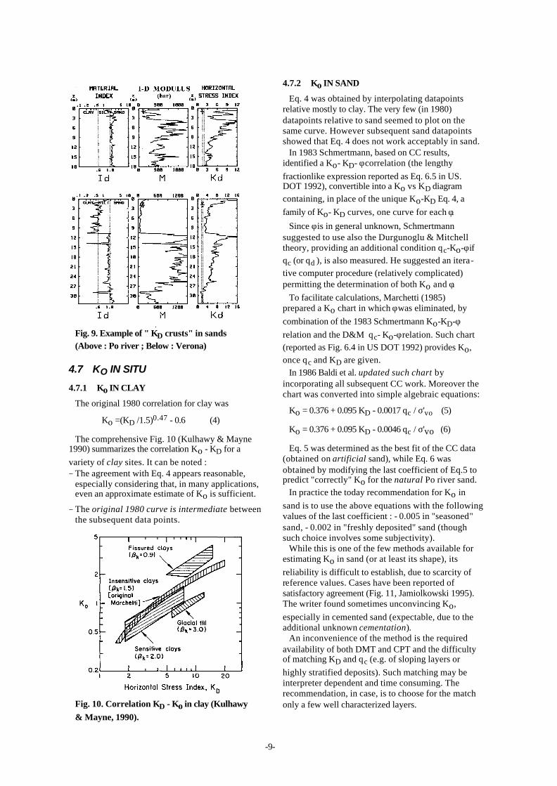
Apart from quantitative estimates, shallow or

buried desiccation crusts in sands appear well highlighted by the KD profile, as exemplified by the " KD crusts" in Fig. 9.

(The shallow " KD crusts" in Fig. 9 are not believed a

consequence of their vicinity to groundsurface, i.e. dilatancy effects, because, if it was so, " KD crusts"

would show up in most sand profiles, which is not the case. Nor is it likely that the Dr variation with depth was such to generate a KD shape so similar to the typical shape of KD in desiccation crusts).

-9-

Fig. 9. Example of " KD crusts" in sands (Above : Po river ; Below : Verona)

4.7 KO IN SITU

4.7.1 Ko IN CLAY

The original 1980 correlation for clay was

Ko =(KD /1.5)0.47 - 0.6 (4)

The comprehensive Fig. 10 (Kulhawy & Mayne 1990) summarizes the correlation Ko - KD for a

variety of clay sites. It can be noted : − The agreement with Eq. 4 appears reasonable,

especially considering that, in many applications, even an approximate estimate of Ko is sufficient.

− The original 1980 curve is intermediate between the subsequent data points.

Fig. 10. Correlation KD - Ko in clay (Kulhawy

& Mayne, 1990).

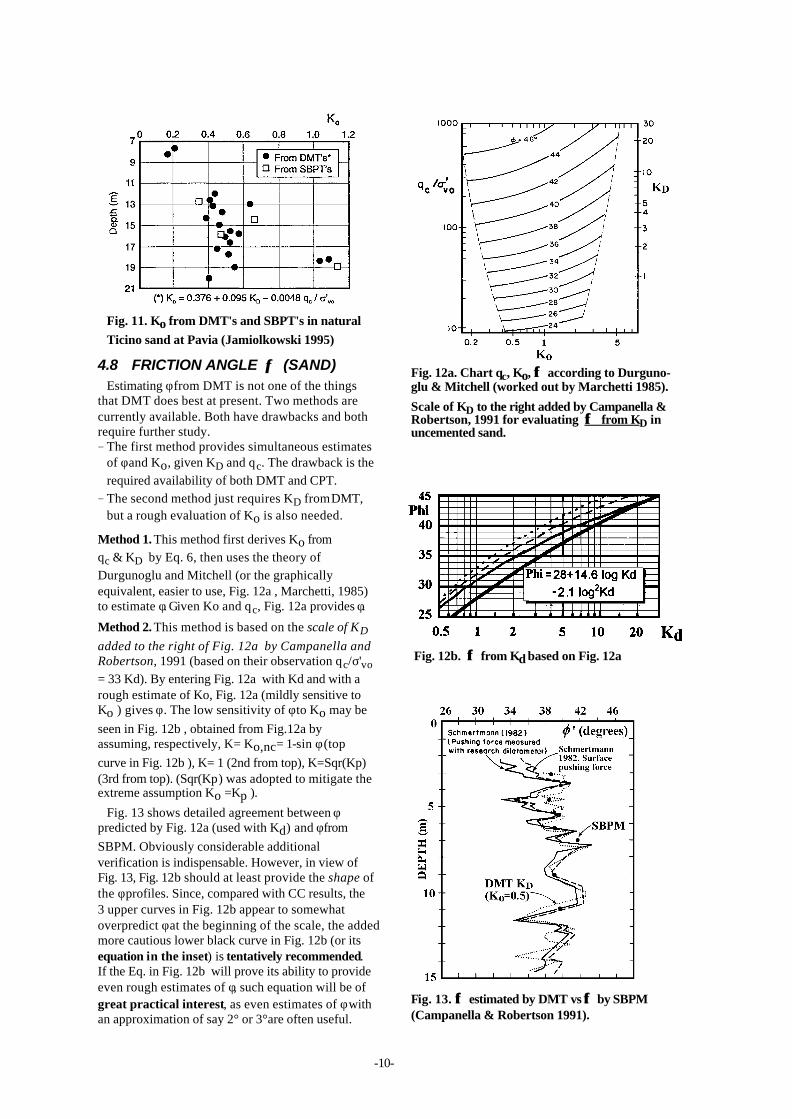
4.7.2 Ko IN SAND

Eq. 4 was obtained by interpolating datapoints relative mostly to clay. The very few (in 1980) datapoints relative to sand seemed to plot on the same curve. However subsequent sand datapoints showed that Eq. 4 does not work acceptably in sand.

In 1983 Schmertmann, based on CC results, identified a Ko- KD- φ correlation (the lengthy

fractionlike expression reported as Eq. 6.5 in US. DOT 1992), convertible into a Ko vs KD diagram

containing, in place of the unique Ko-KD Eq. 4, a

family of Ko- KD curves, one curve for each φ.

Since φ is in general unknown, Schmertmann suggested to use also the Durgunoglu & Mitchell theory, providing an additional condition qc-Ko-φ if

qc (or qd ), is also measured. He suggested an itera-

tive computer procedure (relatively complicated) permitting the determination of both Ko and φ.

To facilitate calculations, Marchetti (1985) prepared a Ko chart in which φ was eliminated, by

combination of the 1983 Schmertmann Ko-KD-φ

relation and the D&M qc- Ko-φ relation. Such chart

(reported as Fig. 6.4 in US DOT 1992) provides Ko,

once qc and KD are given.

In 1986 Baldi et al. updated such chart by incorporating all subsequent CC work. Moreover the chart was converted into simple algebraic equations:

Ko = 0.376 + 0.095 KD - 0.0017 qc / σ'vo (5)

Ko = 0.376 + 0.095 KD - 0.0046 qc / σ'vo (6)

Eq. 5 was determined as the best fit of the CC data (obtained on artificial sand), while Eq. 6 was obtained by modifying the last coefficient of Eq.5 to predict "correctly" Ko for the natural Po river sand.

In practice the today recommendation for Ko in

sand is to use the above equations with the following values of the last coefficient : - 0.005 in "seasoned" sand, - 0.002 in "freshly deposited" sand (though such choice involves some subjectivity).

While this is one of the few methods available for estimating Ko in sand (or at least its shape), its

reliability is difficult to establish, due to scarcity of reference values. Cases have been reported of satisfactory agreement (Fig. 11, Jamiolkowski 1995). The writer found sometimes unconvincing Ko,

especially in cemented sand (expectable, due to the additional unknown cementation).

An inconvenience of the method is the required availability of both DMT and CPT and the difficulty of matching KD and qc (e.g. of sloping layers or

highly stratified deposits). Such matching may be interpreter dependent and time consuming. The recommendation, in case, is to choose for the match only a few well characterized layers.

-10-

Fig. 11. Ko from DMT's and SBPT's in natural

Ticino sand at Pavia (Jamiolkowski 1995)

4.8 FRICTION ANGLE φφ (SAND) Estimating φ from DMT is not one of the things

that DMT does best at present. Two methods are currently available. Both have drawbacks and both require further study. − The first method provides simultaneous estimates

of φ and Ko, given KD and qc. The drawback is the

required availability of both DMT and CPT.

− The second method just requires KD from DMT, but a rough evaluation of Ko is also needed.

Method 1. This method first derives Ko from

qc & KD by Eq. 6, then uses the theory of

Durgunoglu and Mitchell (or the graphically equivalent, easier to use, Fig. 12a , Marchetti, 1985) to estimate φ. Given Ko and qc, Fig. 12a provides φ.

Method 2. This method is based on the scale of KD

added to the right of Fig. 12a by Campanella and Robertson, 1991 (based on their observation qc/σ'vo

= 33 Kd). By entering Fig. 12a with Kd and with a rough estimate of Ko, Fig. 12a (mildly sensitive to Ko ) gives φ . The low sensitivity of φ to Ko may be

seen in Fig. 12b , obtained from Fig.12a by assuming, respectively, K= Ko,nc= 1-sin φ (top

curve in Fig. 12b ), K= 1 (2nd from top), K=Sqr(Kp) (3rd from top). (Sqr(Kp) was adopted to mitigate the extreme assumption Ko =Kp ).

Fig. 13 shows detailed agreement between φ predicted by Fig. 12a (used with Kd) and φ from

SBPM. Obviously considerable additional verification is indispensable. However, in view of Fig. 13, Fig. 12b should at least provide the shape of the φ profiles. Since, compared with CC results, the 3 upper curves in Fig. 12b appear to somewhat overpredict φ at the beginning of the scale, the added more cautious lower black curve in Fig. 12b (or its equation in the inset) is tentatively recommended. If the Eq. in Fig. 12b will prove its ability to provide even rough estimates of φ, such equation will be of great practical interest, as even estimates of φ with an approximation of say 2° or 3°are often useful.

Fig. 12a. Chart qc, Ko, φφ according to Durguno-glu & Mitchell (worked out by Marchetti 1985).

Scale of KD to the right added by Campanella & Robertson, 1991 for evaluating φφ from KD in uncemented sand.

Fig. 12b. φφ from Kd based on Fig. 12a

Fig. 13. φφ estimated by DMT vs φφ by SBPM (Campanella & Robertson 1991).

-11-

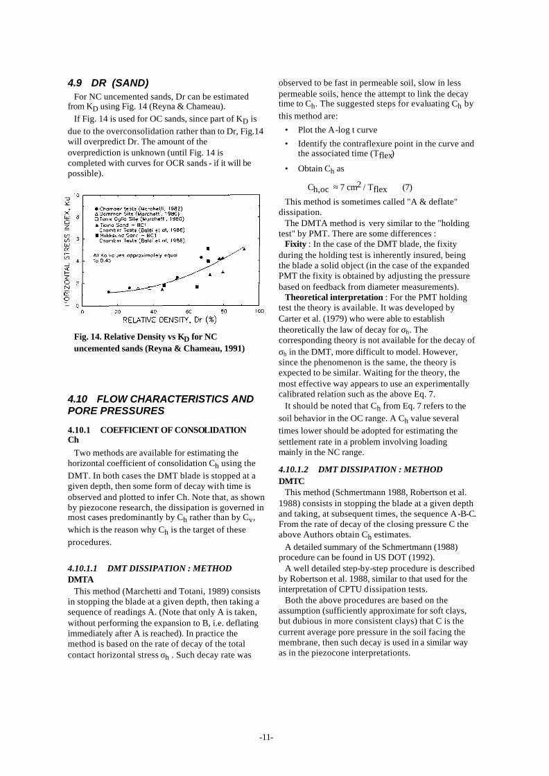
4.9 DR (SAND) For NC uncemented sands, Dr can be estimated

from KD using Fig. 14 (Reyna & Chameau).

If Fig. 14 is used for OC sands, since part of KD is

due to the overconsolidation rather than to Dr, Fig.14 will overpredict Dr. The amount of the overprediction is unknown (until Fig. 14 is completed with curves for OCR sands - if it will be possible).

Fig. 14. Relative Density vs KD for NC uncemented sands (Reyna & Chameau, 1991)

4.10 FLOW CHARACTERISTICS AND PORE PRESSURES

4.10.1 COEFFICIENT OF CONSOLIDATION Ch

Two methods are available for estimating the horizontal coefficient of consolidation Ch using the

DMT. In both cases the DMT blade is stopped at a given depth, then some form of decay with time is observed and plotted to infer Ch. Note that, as shown by piezocone research, the dissipation is governed in most cases predominantly by Ch rather than by Cv,

which is the reason why Ch is the target of these

procedures.

4.10.1.1 DMT DISSIPATION : METHOD DMTA

This method (Marchetti and Totani, 1989) consists in stopping the blade at a given depth, then taking a sequence of readings A. (Note that only A is taken, without performing the expansion to B, i.e. deflating immediately after A is reached). In practice the method is based on the rate of decay of the total contact horizontal stress σh . Such decay rate was

observed to be fast in permeable soil, slow in less permeable soils, hence the attempt to link the decay time to Ch. The suggested steps for evaluating Ch by

this method are:

• Plot the A-log t curve

• Identify the contraflexure point in the curve and the associated time (Tflex)

• Obtain Ch as

Ch,oc ≈ 7 cm2 / Tflex (7)

This method is sometimes called "A & deflate" dissipation.

The DMTA method is very similar to the "holding test" by PMT. There are some differences :

Fixity : In the case of the DMT blade, the fixity during the holding test is inherently insured, being the blade a solid object (in the case of the expanded PMT the fixity is obtained by adjusting the pressure based on feedback from diameter measurements).

Theoretical interpretation : For the PMT holding test the theory is available. It was developed by Carter et al. (1979) who were able to establish theoretically the law of decay for σh. The corresponding theory is not available for the decay of σh in the DMT, more difficult to model. However, since the phenomenon is the same, the theory is expected to be similar. Waiting for the theory, the most effective way appears to use an experimentally calibrated relation such as the above Eq. 7.

It should be noted that Ch from Eq. 7 refers to the

soil behavior in the OC range. A Ch value several

times lower should be adopted for estimating the settlement rate in a problem involving loading mainly in the NC range.

4.10.1.2 DMT DISSIPATION : METHOD DMTC

This method (Schmertmann 1988, Robertson et al. 1988) consists in stopping the blade at a given depth and taking, at subsequent times, the sequence A-B-C. From the rate of decay of the closing pressure C the above Authors obtain Ch estimates.

A detailed summary of the Schmertmann (1988) procedure can be found in US DOT (1992).

A well detailed step-by-step procedure is described by Robertson et al. 1988, similar to that used for the interpretation of CPTU dissipation tests.

Both the above procedures are based on the assumption (sufficiently approximate for soft clays, but dubious in more consistent clays) that C is the current average pore pressure in the soil facing the membrane, then such decay is used in a similar way as in the piezocone interpretationts.

-12-

4.10.2 COEFFICIENT OF PERMEABILITY

Schmertmann and Crapps (1988) suggest the following tentative procedure for deriving Kh from

Ch:

− Estimate Mh using Mh = Ko MDMT , i.e. assuming

M proportional to the effective stress in the desired direction

− Obtain Kh = Ch γw / Mh

4.10.3 ACCURACY OF Ch BY DMT

Given the scarcity of reliable reference values, it is not possible today to evaluate adequately the quality of Ch predicted by DMT. It is only possible to list the

physical reasons why the potentiality of the DMT dissipations appears promising: • The problem of filter smearing or clogging does

not exist with the DMT membrane, because the membrane is anyway a non draining boundary, and what is monitored is a total contact stress (the water flows away from the membrane). Similarly, loss of saturation of the filter is a non-problem in the "bloodless" (dry) DMT dissipations.

• The distortion (turbulence) in the soil surrounding conical tips is more severe.

• Around a cone there is a multiplicity of u(t) decay curves (of different shape). Generally u(t) is measured at one location, but its representativity of u(t) elsewhere is unknown.

• While u(t) vary from point to point, settlements (e.g. under an embankment - the membrane can be regarded as a mini lateral embankment) have a more stable trend, being some kind of integral. The superior stability of Tflex (from DMTA

dissipations) over T50 (CPTU dissipations) is clearly seen in Fig. 6 of the Marchetti & Totani, 1989 paper, hence the superior stability of the inferred Ch.

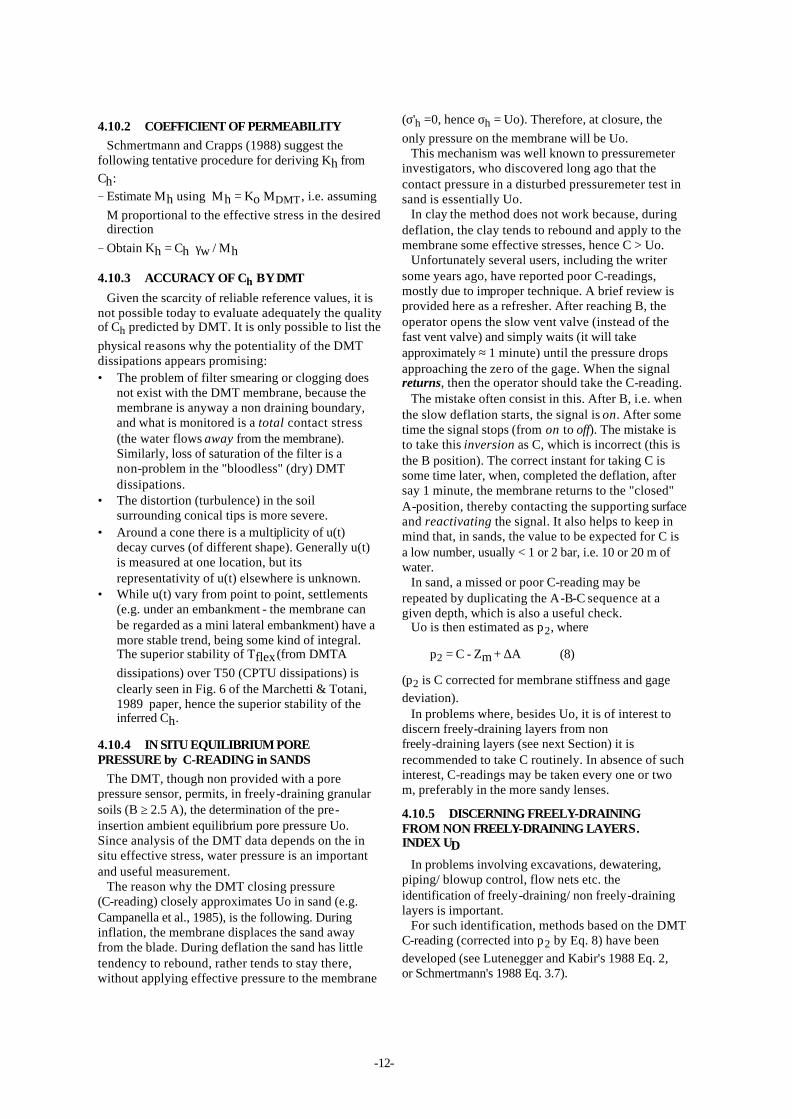
4.10.4 IN SITU EQUILIBRIUM PORE PRESSURE by C-READING in SANDS

The DMT, though non provided with a pore pressure sensor, permits, in freely-draining granular soils (B ≥ 2.5 A), the determination of the pre-insertion ambient equilibrium pore pressure Uo. Since analysis of the DMT data depends on the in situ effective stress, water pressure is an important and useful measurement.

The reason why the DMT closing pressure (C-reading) closely approximates Uo in sand (e.g. Campanella et al., 1985), is the following. During inflation, the membrane displaces the sand away from the blade. During deflation the sand has little tendency to rebound, rather tends to stay there, without applying effective pressure to the membrane

(σ'h =0, hence σh = Uo). Therefore, at closure, the

only pressure on the membrane will be Uo. This mechanism was well known to pressuremeter

investigators, who discovered long ago that the contact pressure in a disturbed pressuremeter test in sand is essentially Uo.

In clay the method does not work because, during deflation, the clay tends to rebound and apply to the membrane some effective stresses, hence C > Uo.

Unfortunately several users, including the writer some years ago, have reported poor C-readings, mostly due to improper technique. A brief review is provided here as a refresher. After reaching B, the operator opens the slow vent valve (instead of the fast vent valve) and simply waits (it will take approximately ≈ 1 minute) until the pressure drops approaching the zero of the gage. When the signal returns, then the operator should take the C-reading.

The mistake often consist in this. After B, i.e. when the slow deflation starts, the signal is on. After some time the signal stops (from on to off). The mistake is to take this inversion as C, which is incorrect (this is the B position). The correct instant for taking C is some time later, when, completed the deflation, after say 1 minute, the membrane returns to the "closed" A-position, thereby contacting the supporting surface and reactivating the signal. It also helps to keep in mind that, in sands, the value to be expected for C is a low number, usually < 1 or 2 bar, i.e. 10 or 20 m of water.

In sand, a missed or poor C-reading may be repeated by duplicating the A-B-C sequence at a given depth, which is also a useful check.

Uo is then estimated as p2, where

p2 = C - Zm + ∆A (8)

(p2 is C corrected for membrane stiffness and gage

deviation). In problems where, besides Uo, it is of interest to

discern freely-draining layers from non freely-draining layers (see next Section) it is recommended to take C routinely. In absence of such interest, C-readings may be taken every one or two m, preferably in the more sandy lenses.

4.10.5 DISCERNING FREELY-DRAINING FROM NON FREELY-DRAINING LAYERS. INDEX UD

In problems involving excavations, dewatering, piping/ blowup control, flow nets etc. the identification of freely-draining/ non freely-draining layers is important.

For such identification, methods based on the DMT C-reading (corrected into p2 by Eq. 8) have been

developed (see Lutenegger and Kabir's 1988 Eq. 2, or Schmertmann's 1988 Eq. 3.7).

-13-

The basis of the method is the following. As discussed in the previous Section, in

freely-draining layers p2 ≈ Uo.

In layers not freely-draining enough to complete the dissipation in the say 1.5 min elapsed since insertion, some excess pore pressure will still exist at the time of the C reading, hence p2 > Uo.

Therefore : p2 = Uo indicates a "freely-draining soil" (= dissipation completed in 1-1.5 min) while p2 > Uo indicates a "non freely-draining soil". The more p2 exceeds Uo, the less permeable is the soil.

Index Ud. Based on the above, the pore pressure

index UD was defined by Lutenegger and Kabir

(1988) as :

UD = (p2-uo) / (po - uo) (9)

In freely-draining soils, where p2 ≈ Uo, UD ≈ 0. In

non freely-draining soils, p2 will be higher then Uo and UD too.

The example in Fig. 15 (Benoit, 1989) illustrates how UD can discern "permeable" layers (UD =0),

"impermeable" layers (UD =0.7) and intermediate

permeability layers (UD between 0 and 0.7), in

agreement with Bq from CPTU. Note that UD , while useful for the above scope,

cannot be expected to offer a scale over the full range of permeabilities. In fact beyond a certain k the test will be drained anyway, below a certain k the test will be undrained anyway.

In layers recognized by UD as non freely-draining,

quantitative evaluation of Ch can be obtained e.g.

using the DMT dissipations described earlier. In layers recognized by UD as freely-draining, the

DMT dissipations will not be performed (the DMT dissipations are not feasible if most of the dissipation occurs in the first minute, because readings cannot be taken in the first ≈ 15 sec).

5. PRESENTATION OF RESULTS Fig. 16 shows the recommended graphical format

of the DMT output. Such output displays 4 profiles, namely Id, M, Cu, KD. This choice is not accidental,

but is the result of a long evolution, resulting from analyzing DMT data at some 500 sites. Experience has shown that these 4 parameters are generally the most significant group to plot (balancing reliability, expressivity, usefulness). Note that KD, though not a

common soil parameter, has been selected as one to be displayed being generally helpful in "understanding" the site history, being similar in shape to the OCR profile.

It is also recommended that the diagrams be presented side by side, and not separated. It is very beneficial for the user to see the diagrams together.

A key question is who should reduce the data and at what point to stop the reduction. Here two viewpoints have to be considered :

(a) If the organization performing the DMTs stops the reduction at ID, KD, ED then it is likely that

errors will be introduced at some later stage, not only by users unfamiliar with DMT reductions, but also by well organized users, just because of the break in the smooth flow of data.

(b) We, as engineers, want to be free to interpret the data ourselves, and strongly dislike some test outputs giving "everything".

The recommendation is that the organization performing the test supplies either ID, KD, ED and

Fig. 15. Use of UD for discerning freely draining layers (UD =0) from non-freely draining (Benoit

1989)

Fig. 16. Recommended graphical presentation of DMT results

-14-

the interpreted parameters (possibly in the recommended graphical format) specifying clearly the correlations used. In many cases the correlations will be the original 1980 correlations, shown often in this reports mostly intermediate between the subsequent data points. Such interpreted parameters can provide a "base" of interpretation. Of course the engineer can later perform a different interpretation by restarting from ID, KD, ED (objective parameters)

using his own correlations. A case in point is the "Settlement of Spread

Footing Prediction", Texas A&M University, (ASCE, 1994). A prediction package, with the re-sults of various field tests, was sent to the predictors.

The writer's group supervised the DMT field work and gave the organizers, for distribution, both ID,

KD, ED, and the interpretations (using the 1980

correlations) of two DMTs. The organizers sent to the participants only the raw data and ID, KD, ED (recalculated by them), without the interpreted MDMT . Unfortunately, in the process, the organizers

mistranscripted the initial test depth for DMT2 (real depth = 1.2 m, wrong depth = 0.2m), so that all the KD they recalculated (and distributed) were also

wrong (list of KD on p. 71 of the Prediction

Symposium Proc., 1994). Hence the predictors, besides lacking the interpreted MDMT , had even to work with the wrong KDs. Result :

− Some predictors, unfamiliar with the reduction, ended up by using ED (confused with a Young's

modulus) instead of M (a gross mistake, see Sections 4.2 and 7.2).

− Some predictors, failing to recognize similarities between DMT1 and DMT2 (largely mislead by the wrong depth and the ensuing wrong KD), explained

the lack of similarity with the "inherent non-reproducibility of sands and the inevitable vagaries in such soils".

Fig. 17 . Profiles of M obtained in sand by two DMTs at the prediction tests site (Texas A&M)

Had the organizers distributed Fig. 17 (included in the documents given by the writer to Texas A&M for distribution - believed a remarkable example of reproducibility in sand) every interested predictor could have produced classical settlement predictions using M in the usual ways. Rest of the story :

Footing 3x3 m : Eq. 10, with MDMT in Fig. 17,

predicts 4.8 mm/bar, which, after a footing rigidity correction of 0.8, becomes 3.84 mm/bar. Hence, to cause the "working conditions" settlement 0.5% B (Section 8.1), equal to 15 mm, a load of 3.91 bar has to be applied, i.e. 3519 KN on a 9 m2 footing. Thus for a 3519 KN load S1-DMT =15 mm, while

Sobserved (Fig. 3 on p. 97 of ASCE, 1994),was 12 mm, with an S1-DMT overprediction of +25%.

Footing 1.5x1.5 m.: Similarly, for an applied load of 844 KN, S1-DMT = 7.5 mm (0.5% B), vs Sobserved

= 6.5 mm (Fig. 6 on p. 100 of ASCE, 1994), with a +15% overprediction.

6. DISTORTIONS CAUSED BY THE PENETRATION

Fig. 18 compares the distortions caused by conical tips and by wedges. It can be noted:

Fig. 18 . Deformed grids by Baligh & Scott (1975)

-15-

− Distortions are considerably lower for wedges, reducing the amount of back-extrapolation needed to infer pre-penetration soil properties.

− The cone penetration creates considerable turbulence. The strain pattern bears no resemblance to that of a cylindrical cavity expansion (that would produce a deformed grid made of vertical and horizontal lines), as assumed in many theoretical studies.

− The strain produced by conical tips should not be of concern when looking for strength, but perhaps makes it difficult to investigate compressibility.

7. SPECIAL CONSIDERATIONS

7.1 SOME COMMENTS ON THE CURRENT ROLE OF INSITU TESTING

An interesting view on the today role of insitu testing was expressed by Schmertmann at the banquet talk at the Symposium CPT '95 in Sweden.

"I believe that...while in the past the laboratory had a primary role in a site investigation, and in situ testing a complementary role...we have reached a stage where in situ has a primary role, and the laboratory a complementary role".

Schmertmann cited as an example the Sunshine Skyway Suspension Tampa Bridge, where Schmertmann & Crapps were responsible for the geotechnical design. He reported that 99% of the testing was run in situ, 1% in the laboratory (and the reason of the 1% in the laboratory was to avoid colleague criticism).

(Of course audience and speaker were well aware that the laboratory is the central source of our basic understanding, including insitu tests).

If the trend towards insitu testing continues, it is foreseeable that more and more investigations will consist of penetration tests, fast, economical, reproducible. In simple problems involving only soil rupture it is possible that CPT alone will suffice. In problems involving deformations and stress state, also tests able to provide such information will be used.

In many practical cases the availability of the 3 independent determinations

qc (CPT) KD (DMT) M(DMT)

should represent a respectable base of information. 7.2 PARAMETER DETERMINATION BY "TRIANGULATION"

Unlike laboratory tests, in situ tests are generally unable to measure "pure" soil properties. In situ tests generally provide responses which are a mixed function of such "pure" soil properties. In order to isolate them, it is necessary a "triangulation".

Say that dominant soil information are : stiffness, strength, state of stress. Hence three independent responses are needed. Conceptually:

R1 = f1 (M, Strength, σh)

R2 = f2 (M, Strength, σh)

R3 = f3 (M, Strength, σh)

Invert matrix and get

M

Strength

σh

=

=

=

g1 (R1,R2,R3)

g2 (R1,R2,R3)

g3 (R1,R2,R3 )

MDMT is along these lines, being obtained as a function of ID , KD , ED (though only two are

independent parameters - see Section 4 ). It is foreseeable that in the future we shall see more "triangulations".

The above concepts explain the previous recommendation to avoid correlations with ED alone, i.e. not in combination with other parameters. In particular ED lacks information on stress history. Hence ED should only be used in combination with KD (and ID) to get M. Then, if

Young's modulus E' is needed, it can be estimated as E' ≈ 0.8 M

7.3 DRAINAGE CONDITIONS DURING THE DILATOMETER TEST

In a clean sand the DMT is a perfectly drained test. Both excess pore pressures ∆u (∆u,penetration and ∆u,expansion) are virtually zero throughout the test, whose duration (say 1 min) is sufficient for any excess to dissipate.

In a low permeability clay the opposite is true, i.e. the test is undrained and the excesses do not undergo any appreciable dissipation.

It should be noted, however, that, for opposite reasons, at any given time, the pore pressure distribution around the blade is constant in both cases. In the drained case the pore pressure is everywhere Uo (the equilibrium pore pressure), in the undrained case the pore pressures do not vary (in absence of movement).

There is however a niche of soils (in the silts region) for which 1 min is insufficient for full drainage, but sufficient to permit some dissipation. In these partial drainage soils the data obtained can be misleading to an unaware user. In fact the reading B, which follows A by say 15 sec, is not the "proper match" of A, because in the 15 sec from A to B, excess has been dissipating and B is too low, with the consequence that the difference B-A is also too low and so are the derived values Id, Ed, M. In such soils ID will possibly end up in the extreme left hand

of its scale (ID =0.1 or less) and M will also show, at

least occasionally, very low values.

-16-

This situation is not very frequent, the writer noted it only in two sites so far (Drammen clay-Norway and and Garigliano clay-Italy).

To be sure, in case of very low ID and M, there is

some ambiguity because the low values of B-A could just be the normal response of a low permeability very soft clay. The ambiguity can be solved with the help of C-readings (or UD - Section 4.10.5, Eq. 9). If

the UD values in the "low B-A" layers are

intermediate between those found in the free-draining layers and those found in the non free-draining layers, than the above interpretation of partial drainage is presumably correct. Of course the partial drainage explanation can also be verified by means of laboratory sieve analysis or permeability tests.

In practice, if the partial drainage explanation of the low B-A is confirmed, all results dependent from B-A (recognizable by very depressed ID troughs)

have to be ignored.

8. APPLICATION TO ENGINEERING PROBLEMS

As mentioned earlier, the primary way of using DMT results is "design via parameters".

However this Section provides some details on the use of DMT in some specific applications.

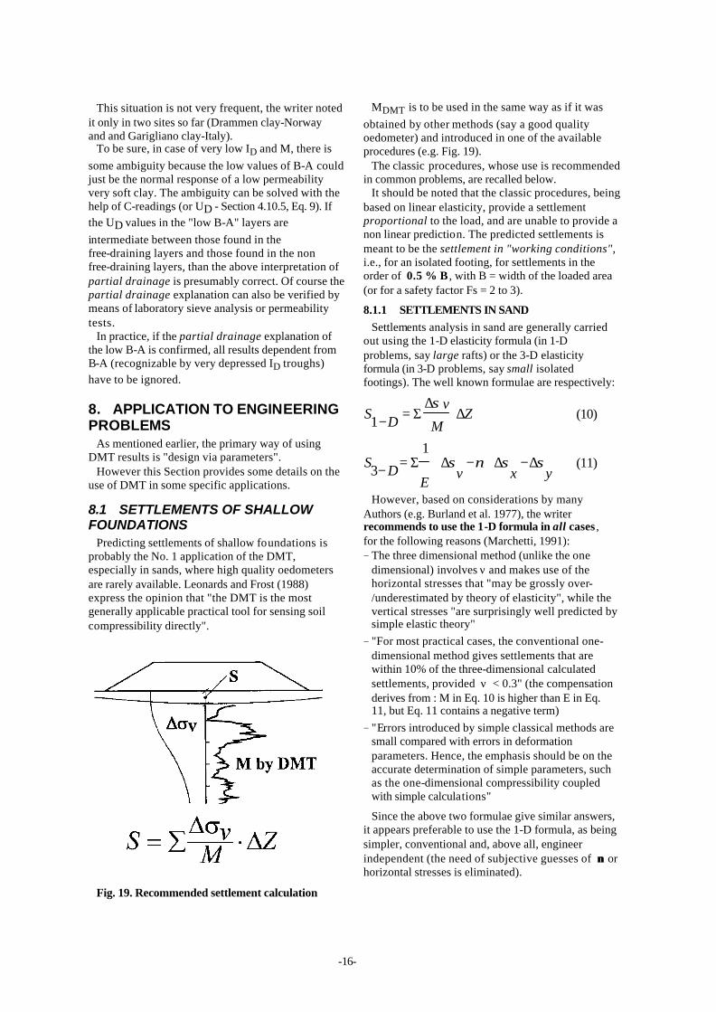
8.1 SETTLEMENTS OF SHALLOW FOUNDATIONS

Predicting settlements of shallow foundations is probably the No. 1 application of the DMT, especially in sands, where high quality oedometers are rarely available. Leonards and Frost (1988) express the opinion that "the DMT is the most generally applicable practical tool for sensing soil compressibility directly".

Fig. 19. Recommended settlement calculation

MDMT is to be used in the same way as if it was

obtained by other methods (say a good quality oedometer) and introduced in one of the available procedures (e.g. Fig. 19).

The classic procedures, whose use is recommended in common problems, are recalled below.

It should be noted that the classic procedures, being based on linear elasticity, provide a settlement proportional to the load, and are unable to provide a non linear prediction. The predicted settlements is meant to be the settlement in "working conditions", i.e., for an isolated footing, for settlements in the order of 0.5 % B , with B = width of the loaded area (or for a safety factor Fs = 2 to 3).

8.1.1 SETTLEMENTS IN SAND

Settlements analysis in sand are generally carried out using the 1-D elasticity formula (in 1-D problems, say large rafts) or the 3-D elasticity formula (in 3-D problems, say small isolated footings). The well known formulae are respectively:

SD

v

MZ

1− = ⋅Σ∆

∆σ

(10)

SD

Ev x y3

1

− = ⋅ − ⋅ −

Σ ∆ ∆ ∆σ ν σ σ (11)

However, based on considerations by many Authors (e.g. Burland et al. 1977), the writer recommends to use the 1-D formula in all cases , for the following reasons (Marchetti, 1991): − The three dimensional method (unlike the one

dimensional) involves ν and makes use of the horizontal stresses that "may be grossly over-/underestimated by theory of elasticity", while the vertical stresses "are surprisingly well predicted by simple elastic theory"

− "For most practical cases, the conventional one-dimensional method gives settlements that are within 10% of the three-dimensional calculated settlements, provided ν < 0.3" (the compensation derives from : M in Eq. 10 is higher than E in Eq. 11, but Eq. 11 contains a negative term)

− "Errors introduced by simple classical methods are small compared with errors in deformation parameters. Hence, the emphasis should be on the accurate determination of simple parameters, such as the one-dimensional compressibility coupled with simple calculations"

Since the above two formulae give similar answers, it appears preferable to use the 1-D formula, as being simpler, conventional and, above all, engineer independent (the need of subjective guesses of νν or horizontal stresses is eliminated).

-17-

In case it is opted for the use of the 3-D formulae, E can be derived from M using the theory of elasticity, that, for ν = 0.25, provides E = 0.83 M (a factor not very far from unity). Indeed M and E are often used interchangeably in view of the involved approximation.

8.1.2 SETTLEMENTS IN CLAY

The primary settlement in clay is usually calculated by the classic log formulae using the coefficients Cc and Cr determined by oedometer tests. Alternatively, and with similar results, the settlement are calculated using the average Eoed derived from the laboratory curve in correspondence of the expected stress range.

Since DMT provides M rather Cc and Cr, the method to be used is the second one, resulting again in the use of Eq. 10.

If E' of the clay skeleton is required, it can be obtained as E' ≈ 0.8 M.

It should be noted that in some highly structured clays, whose oedometer curves exhibit a sharp break and a dramatic fall in slope across the preconsolidation pressure pc, M from DMT could

be an inadequate average if the loading straddles pc.

However in many common clays, and probably in most sands, the M fluctuation across pc is mild, and

M can be considered an adequate average modulus.

8.1.3 MANIPULABILITY OF THE CALCULATED SETTLEMENT

A distinct characteristic of S1-DMT (the result of Eq. 10 when MDMT is used) is that S1-DMT is the end

product of a seamless non subjective chain, from in situ to the office. In fact: − Field raw data are independent from operator

− The factor for converting ED to M is not chosen by

the person making interpretation, but is obtained as RM =M / ED =f (ID, KD)

− S1-DMT is independent from the person calculating

the settlements

This non manipulability facilitates accumulation of consistent comparative data.

To be sure, in 3-D problems in OC clays, some margin of manipulation still exists and should be kept under control. As said earlier, S1-DMT is to be

treated as if it was obtained by using Eoed. Therefore

if S1-DMT is used to predict the primary settlement, S1-DMT should still be corrected for rigidity, depth,

Skempton-Bjerrum correction. While the rigidity correction (if applicable, typically 0.8) and the depth correction (if applicable, typically 0.8 to 1) are near unity, hence no substantial, in 3-D problems in OC clays the correction factor could often be 0.2 to 0.5 (<<1). "According to the book" the latter correction should be applied. However considering that :

− The application of the Skempton-Bjerrum correction is equivalent to reducing S1-DMT by a factor 2 to 5

− Terzaghi & Peck's book states that "if the applied load exceeds pc, the modulus from even good

oedometers may be 2 to 5 times smaller than the in situ modulus"

these two factors approximately cancel out. Therefore, pending a specific study on this

particular condition, the writer is in favor of adopting as primary settlement Sc (even in 3-D problems in

OC clays) directly S1-DMT from Eq. 10, without the

Skempton-Bjerrum correction (while adopting, if applicable, the rigidity and the depth corrections).

The resilience of S1-DMT to manipulation is of

course no prove of accuracy, it simply facilitates comparisons. Accuracy forms the object of next Section.

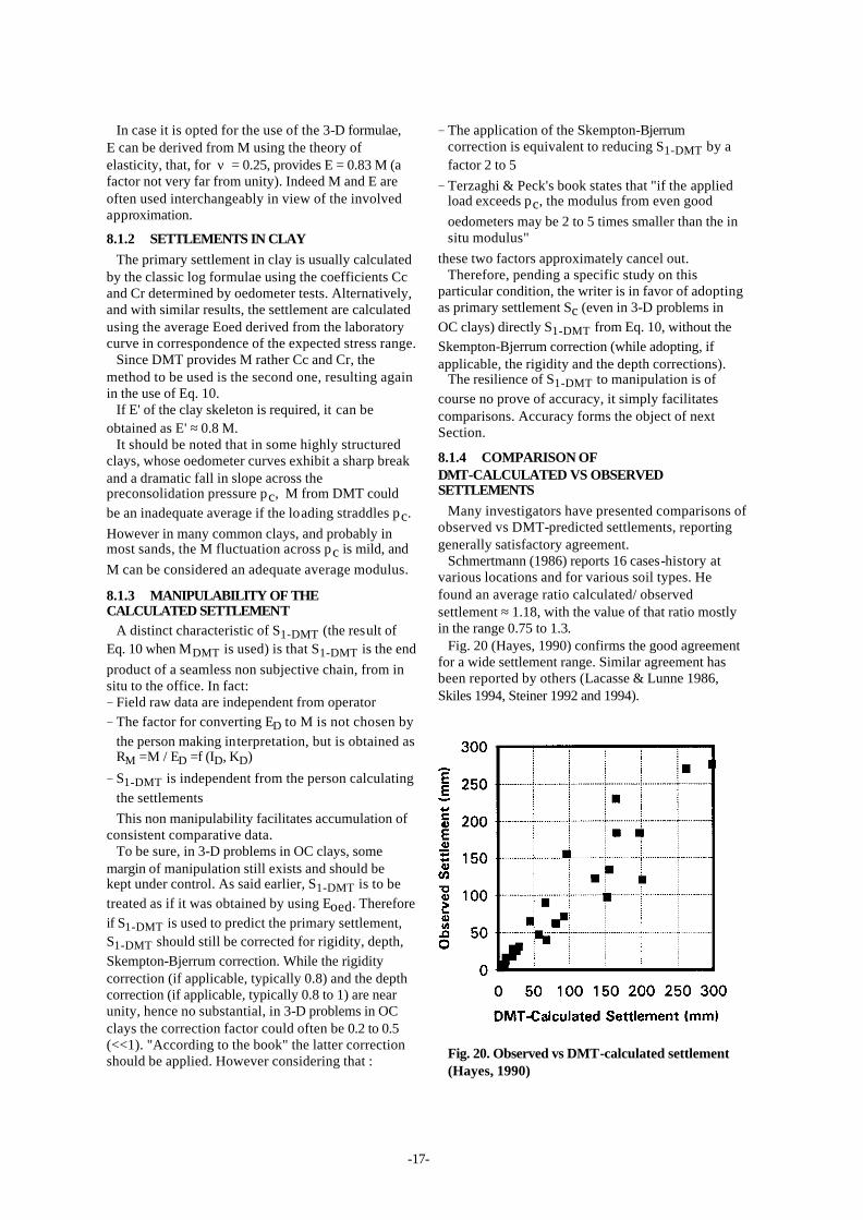
8.1.4 COMPARISON OF DMT-CALCULATED VS OBSERVED SETTLEMENTS

Many investigators have presented comparisons of observed vs DMT-predicted settlements, reporting generally satisfactory agreement.

Schmertmann (1986) reports 16 cases-history at various locations and for various soil types. He found an average ratio calculated/ observed settlement ≈ 1.18, with the value of that ratio mostly in the range 0.75 to 1.3.

Fig. 20 (Hayes, 1990) confirms the good agreement for a wide settlement range. Similar agreement has been reported by others (Lacasse & Lunne 1986, Skiles 1994, Steiner 1992 and 1994).

Fig. 20. Observed vs DMT-calculated settlement (Hayes, 1990)

-18-

8.2 VERTICALLY LOADED PILES

8.2.1 BORED PILES

No special method has been developed for the design of bored piles. (An exception is the method developed by Peiffer for screw piles, described in a next Section, applicable even to bored piles). Therefore the design of bored piles using DMT is generally carried out via soil parameters.

8.2.2 DRIVEN PILES

8.2.2.1 THE DMT-σσhc METHOD This method (Marchetti et al. 1986) was developed

for the case of piles driven in clays. The method is based on the determination of σ'hc (effective

horizontal stress against the DMT blade at the end of the reconsolidation). Then a ρ factor is applied to σ'hc , and the product is used as an estimate of the pile skin friction fs. The method has deep conceptual

roots, being an application of concepts and theories developed by Baligh (1985). However the method has two drawbacks : (a) In clays, the determination of σ'hc can take considerable time (the reconso-

lidation around the blade of impermeable clays can take many hours if not one or two days) which makes the σ'hc determination expensive, especially

in offshore investigations for offshore piles (b) The ρ factor has been found to be not a constant, but a rather variable factor (mostly in the range 0.10 to 0.20). Therefore, until methods for guiding the selection of are developed, the uncertainty in fs is too wide. Nevertheless, in important jobs, the method could helpfully be used to supplement other methods, e.g. for getting information on the shape of the fs profile, or to establish a floor value to fs..

8.2.2.2 HORIZONTAL PRESSURE AGAINST PILES DRIVEN IN CLAY DURING INSTALLATION

Totani et al. (1994) report a finding of practical interest for the engineers deciding the thickness of the shell of mandrel-driven piles in clay. These investigators describe measurements of σh (total) on

a pile driven in a lightly OC clay. The pile was instrumented with 12 total pressure cells, frequently measured during driving. At each depth the pressure σh against the pile was found to be "exactly equal" to po determined by a normal DMT. This finding is in

accordance to theoretical findings by Baligh (1985), predicting σh independent from the dimensions of

the penetrating object (these results suggest independence of σh even from the shape).

8.2.2.3 WARNING OF LOW SKIN FRICTION IN CALCAREOUS SAND

Some calcareous sands are known to generate very low friction on pile shaft, with the consequence of

unusually low pile bearing capacity for lateral friction. Methods for predicting skin friction in such sands are currently not available. However DMTs performed in calcareous sand (Fig. 21) indicate an unusually low KD in such sands. This suggests

− The low fs in these sands is largely due to low σ'h

− The low KD measured by DMT in calcareous sands

is a potentially useful warning for expecting a low friction capacity.

Fig. 21. DMT results in the Plouasne (Brittany) calcareous sand

8.2.3 SCREW PILES

Peiffer (1997) developed a method for estimating the shaft friction of Atlas screw piles based on po

from DMT. The DMT is run in the usual way, but should be performed next to the pile (1 D away from the shaft) after its execution.

Peiffer's method is intermediate between a real design method and a pile load test. It is not a real design method because the estimates are obtained after the pile is executed, nor is it a load test because the bearing capacity is estimated from soil properties and not by loading the pile.

Actually the Peiffer method follows the inescapable logic dictated by some well established facts. It is widely recognized that pile capacity largely depends on execution - besides soil type. Hence one cannot pretend to estimate the pile bearing capacity based only on measurements on the original soil, but should more rationally base such estimates on measurements on the soil after the installation.

This method, though developed for screw piles (and a variety of other piles, all aimed to avoiding soil decompression), is in principle applicable also to bored piles, because the relaxation due to the installation will anyway be incorporated in the after-the-pile DMT results.

-19-

8.3 LATERALLY LOADED PILES Methods have been developed for deriving p-y

curves from DMT results. In particular the writer recommends the papers by Robertson et al. (1987) and by Marchetti et al. (1991).

Robertson 1987 (the reader interested in using the method in design is advised to procure the full paper) clearly illustrates all the steps to estimate p-y curves, both for sands and clays. Validations of the Robertson 1987 method by Marchetti et al. (1991) indicated remarkably good agreement between predicted and observed behavior (first time loading).

Marchetti et al. (1991) streamlined the Robertson method for clay (anchored to the Skempton ε 50 -

Matlock cubic parabola approach), and proposed a more direct procedure for predicting the p-y curves (only for clay). However, since the accuracy appears similar, use of the Robertson method (covering also sands) is adequate.

The p-y curves derived using these methods are the end product of a non subjective chain from in situ to the office. Actually the DMT was originally conceived for the objective determination of the parameters needed for this problem.

Various investigators have stressed the ability of the DMT to obtain considerable data even at shallow depths, i.e. in the layers dominating pile response. Detailed chapters on the use of DMT in this application can be found in Lunne et al. (1989) and US DOT (1992).

An extensive verification program of the existing methods vs observed lateral pile behavior (Project Brite Euram II) is currently in progress, lead and coordinated by NGI, by a group including Boyle, Lunne and Mokkelbost.

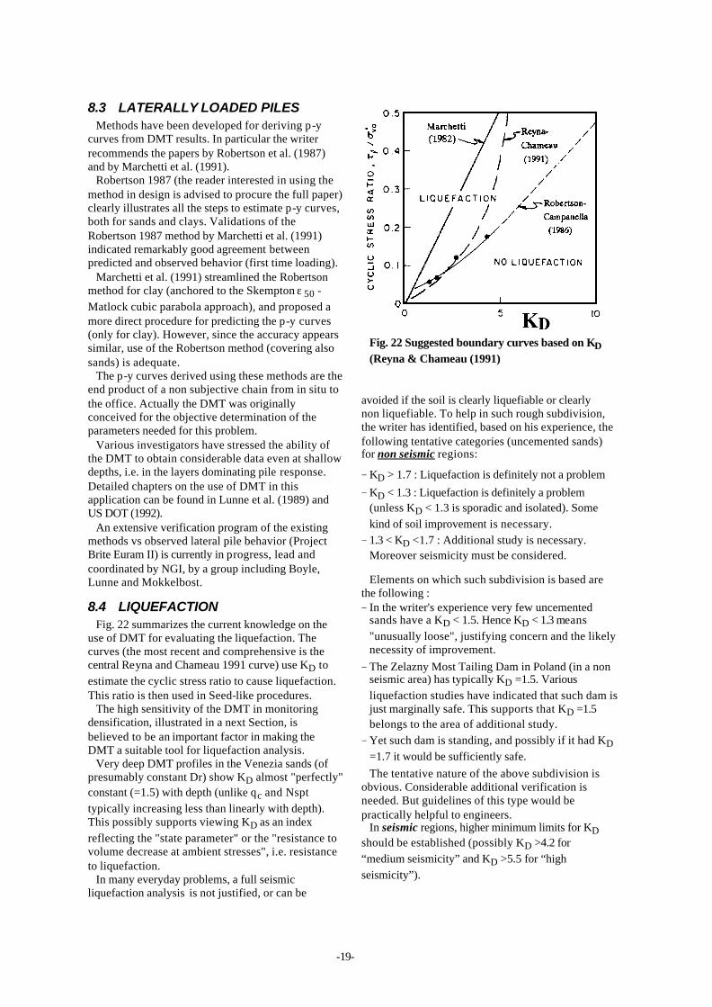
8.4 LIQUEFACTION Fig. 22 summarizes the current knowledge on the

use of DMT for evaluating the liquefaction. The curves (the most recent and comprehensive is the central Reyna and Chameau 1991 curve) use KD to

estimate the cyclic stress ratio to cause liquefaction. This ratio is then used in Seed-like procedures.

The high sensitivity of the DMT in monitoring densification, illustrated in a next Section, is believed to be an important factor in making the DMT a suitable tool for liquefaction analysis.

Very deep DMT profiles in the Venezia sands (of presumably constant Dr) show KD almost "perfectly" constant (=1.5) with depth (unlike qc and Nspt

typically increasing less than linearly with depth). This possibly supports viewing KD as an index

reflecting the "state parameter" or the "resistance to volume decrease at ambient stresses", i.e. resistance to liquefaction.

In many everyday problems, a full seismic liquefaction analysis is not justified, or can be

Fig. 22 Suggested boundary curves based on KD (Reyna & Chameau (1991)

avoided if the soil is clearly liquefiable or clearly non liquefiable. To help in such rough subdivision, the writer has identified, based on his experience, the following tentative categories (uncemented sands) for non seismic regions:

− KD > 1.7 : Liquefaction is definitely not a problem

− KD < 1.3 : Liquefaction is definitely a problem (unless KD < 1.3 is sporadic and isolated). Some

kind of soil improvement is necessary.

− 1.3 < KD <1.7 : Additional study is necessary. Moreover seismicity must be considered.

Elements on which such subdivision is based are the following : − In the writer's experience very few uncemented

sands have a KD < 1.5. Hence KD < 1.3 means

"unusually loose", justifying concern and the likely necessity of improvement.

− The Zelazny Most Tailing Dam in Poland (in a non seismic area) has typically KD =1.5. Various

liquefaction studies have indicated that such dam is just marginally safe. This supports that KD =1.5 belongs to the area of additional study.

− Yet such dam is standing, and possibly if it had KD

=1.7 it would be sufficiently safe.

The tentative nature of the above subdivision is obvious. Considerable additional verification is needed. But guidelines of this type would be practically helpful to engineers.

In seismic regions, higher minimum limits for KD should be established (possibly KD >4.2 for

“medium seismicity” and KD >5.5 for “high

seismicity”).

-20-

8.5 DETECTING SLIP SURFACES IN OVERCONSOLIDATED CLAY SLOPES

Totani et al. (1997) developed a quick method for detecting slip surfaces in overconsolidated clay slopes, based on the inspection of the KD profiles.

The method is based on the following two elements: (a) The sequence of sliding, remo ulding and

reconsolidation (illustrated in Fig. 23) generally leaves the clay in the slip zone(s) in a (nearly) NC state, with loss of structure, ageing or cementation.

(b) Correlations established by several researchers in many different clays have shown that in genuinely NC clays (no structure, ageing or cementation) the horizontal stress index KD from the DMT is approximately equal to 2.

Therefore if an OC clay slopes contains layers with KD ≈ 2, then these layers are likely to be part of a

slip surface (active or quiescent). In essence, the method consists in identifying zones of NC clay in a slope, which, otherwise, exhibits an OC profile, using KD ≈2 as the identifier of the NC zones.

Fig. 23. Detecting slip surfaces in OC clays by means of DMT- KD (Totani et al., 1997)

The method was validated by inclinometers. A point considered of interest is that the method

involves looking for a specific numerical value KD ≈2 rather than simply searching for weak zones,

which could be located just as easily by means of other in situ tests.

Some practical conclusion given in that paper are: − The method provides a faster response than

inclinometers in locating slip surfaces.

− The method enables to quickly detect even quiescent slip surfaces (not revealed by inclinome-ters), which may be reactivated by fresh activity.

− On the other hand the proposed method itself cannot establish if a slope is presently moving and what the movements are, while inclinometer can.

− In many cases, DMT and inclinometers could helpfully be used in combination.

Confirmation KD,NC ≈≈ 2 for genuine NC clays as byproduct of the slip surface research.

A byproduct of the above slip surface research was the confirmation of the value KD, NC ≈ 2 for genuine NC clays. In fact

− In all the layers where sliding was confirmed by inclinometers, it was found KD ≈ 2.

− The clay in the remolded sliding band has certainly lost any trace of ageing, structure, cementation, i.e. such clay is a good example of genuine NC clay

Thus KD ≈ 2 appears the floor value for KD,NC . If a geologically NC clay has KD > 2, any excess of KD

above 2 is a signal of one or more of the above effects (ageing, structure, cementation).

8.6 MONITORING DENSIFICATION / STRESS INCREASE

DMT has been frequently used for monitoring soil improvement, by comparing DMT results before and after the treatment. Compaction is reflected by a brisk increase of both KD and M. However, since

often treatments aim to reducing settlements, specifications are generally set in terms of minimum M values.

Schmertmann (1986) reports a large number of before-after CPTs and DMTs carried out for monitoring dynamic compaction at a power plant site (mostly sand). The treatment increased substantially both qc and MDMT , but the increase in MDMT was

found to be approximately twice the increase in qc.

Jendeby (1992) reports before-after CPTs and DMTs carried out for monitoring the deep compaction produced in a loose sand fill with the "vibrowing". He found a substantial increase of both qc and MDMT , but MDMT increased at a faster rate

(nearly twice), a result similar to the previous case. Higher sensitiv\ity of MDMT , compared with qc,

was reported by Pasqualini and Rosi (1993) in monitoring a vibroflotation treatment. These Authors also noted that the DMT clearly detected the improvement even in layers marginally influenced by the treatment, where the benefits were undetected by CPT.

DMT has also been used extensively by Ghent investigators Peiffer, Van Impe, Cortvrindt and Bottiau for comparing soil changes caused by various pile installation methods. For instance De Cock et al. (1993) describe the use of before-after DMTs to verify, in terms of KD, the installation

-21-

Fig. 24. DMTs before-after for comparing soil changes caused by the installation of various piles (here an Atlas pile). DeCock et al. 1993.

effects of the Atlas pile (Fig. 24). Before-after CPTs were also used, but the Authors concluded that "the DMTs before and after pile installation demonstrate more clearly [than CPT] the beneficial result of the displacement effect of the Atlas pile".

All the above results concurrently suggest that the DMT is uniquely sensitive even to slight changes of stresses/ density in the soil and therefore is particularly suitable when the expected changes are so small that they cannot be detected by other common in situ test.

Sawada and Sugawara (1995) used both SBPM and DMT for comparing the effectiveness of three types of densification methods. They found both SBPM and DMT effective verification tools, and pointed out the convenience of the DMT in view of the low time and cost involved.

Stationary DMT as pressure sensing elements DMT blades have also been used to sense

variations in stress state/ density using them not as penetration tools, but as stationary spade cells. In this application DMT blades are inserted at the levels where changes are expected, then readings (only A) are taken with time.

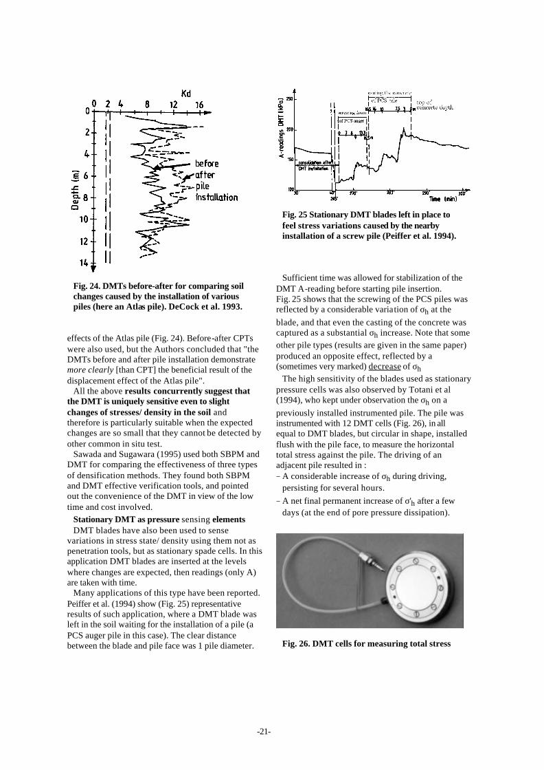
Many applications of this type have been reported. Peiffer et al. (1994) show (Fig. 25) representative results of such application, where a DMT blade was left in the soil waiting for the installation of a pile (a PCS auger pile in this case). The clear distance between the blade and pile face was 1 pile diameter.

Fig. 25 Stationary DMT blades left in place to feel stress variations caused by the nearby installation of a screw pile (Peiffer et al. 1994).

Sufficient time was allowed for stabilization of the DMT A-reading before starting pile insertion. Fig. 25 shows that the screwing of the PCS piles was reflected by a considerable variation of σh at the

blade, and that even the casting of the concrete was captured as a substantial σh increase. Note that some

other pile types (results are given in the same paper) produced an opposite effect, reflected by a (sometimes very marked) decrease of σh

The high sensitivity of the blades used as stationary pressure cells was also observed by Totani et al (1994), who kept under observation the σh on a

previously installed instrumented pile. The pile was instrumented with 12 DMT cells (Fig. 26), in all equal to DMT blades, but circular in shape, installed flush with the pile face, to measure the horizontal total stress against the pile. The driving of an adjacent pile resulted in : − A considerable increase of σh during driving,

persisting for several hours.

− A net final permanent increase of σ'h after a few days (at the end of pore pressure dissipation).

Fig. 26. DMT cells for measuring total stress

-22-

Concerning DMT blades used as stationary pressure cells, it may be noted that, while able to detect stress variations, they do not provide absolute estimates of the stresses before and after construction, in contrast with before-after continuous DMTs. Moreover a stationary blade can only provide information at one location. Yet there are a number of applications in which practical reasons make them preferable.

8.7 MONITORING DENSIFICATION / STRESS DECREASE

The DMT has been used not only to feel the increase, but also the possible reduction of density or horizontal stress.

Peiffer and his colleagues, as mentioned in the previous Section, used the DMT to monitor the decompression caused by various types of piles.

Some investigators (e.g. Hamza, 1995 for Cairo Metro works) have used before-after DMT to get information on the decompression caused by the execution of diaphragm walls.

The use of before-after DMT has been proposed (but not used yet) for monitoring the (probably small) decompression effects of microboring (the technique consisting in boring inclined holes under a tilting buildings to induce settlements in the less sinking side). This use appears particularly apt (even in view of the high sensitivity of DMT), for mapping the soil volume influenced by the treatment. Less straightforward appears the interpretation in terms of Ko decrease.

8.8 SUBGRADE COMPACTION CONTROL

Some experience exists on the use of DMT for evaluating the suitability of the compacted groundsurface (i.e. the subgrade soil) to support the road superstructure (subbase, base, pavements).

Borden (1986), based on laboratory work on molds and large calibration chamber, involving A-2-4 to A-7-5 soils, tentatively suggested to estimate CBR% (corrected, unsoaked) as :

CBR% = 0.058 ED (bar)-0.475 (12)

Marchetti (1994) describes the use of DMT as a fast acceptance tool for the subgrade compaction in a 90 km road in Bangladesh. The procedure was the following: − Perform a few preliminary DMTs in the accepted

subgrade (i.e. satisfying the conventional specifications)

− Based on such preliminary MDMT profiles, define a suitable average MDMT profile, to be used as the

acceptance profile (such profile should indicate explicitly MDMT,MAX )

For the mentioned road the original specifications for the subgrade were : (a) 95% of modified Proctor (b) CBR = 10 (c) Eplate (0.5-1.5 bar) = 300 bar.

These specifications, after the preliminary DMTs in accepted areas, were converted into the MDMT

equivalent acceptance profile in Fig. 27. The DMT could then be used as an economical production method for quality control of the compaction, with only occasional verifications. DMT testing was very fast (60 DMT profiles to a depth of 2-3 m, at 10 cm depth intervals, in 4 days) and avoided a large number of time consuming and tiresome laboratory and insitu CBR tests and plate load tests.

Interestingly, all the after-compaction MDMT

profiles had the typical shape of the profile shown in Fig. 27, with the maximum MDMT found almost

invariably at 25-26 cm depth. It would be helpful to engineers the availability of

acceptance profiles similar to Fig. 27 but applicable to roads of various classes.

Cases have been reported of after construction checks with the blade penetrating directly through asphalt.

Fig. 27. MDMT acceptance profile as a fast method for verifying compaction of subgrade

9. CORRELATION WITH PARAMETERS OBTAINED BY OTHER IN SITU TESTS RELATION DMT / SPT

According to Schmertmann & Crapps (1988): − The estimation of NSPT from DMT would be a

"gross misuse of the DMT data"

− Any such correlation depends on soil type and is probably site specific, and should always be confirmed before use in design

− When using such correlation the engineer should be aware of the high variation in SPT blowcount

− Datapoints expressing graphically a possibly site specific correlation for the Gainesville FL area indicate the following

NSPT = M(bar) / 40 (13)

-23-

RELATION DMT / PMT Some information exists about the relation between

DMT and PMT parameters. Cross correlations, if existing and available, would be of great practical value to the engineer, permitting to tap into the vast experience accumulated, especially by French Engineers, on the use of PMT data to practical applications (design of footings, piles etc.). Preliminary indications suggest :

po/pL ≈ 0.8 (Schmertmann, 1987) (14)

Epmt ≈ 0.4 ED(Kalteziotis et al. 1991) (15)

Dumas (1992) used the DMT in a verification testing of a Dynamic Compaction project. The settlement calculated with DMT was in good agreement with that calculated with the PMT.

Ortigao et al. (1996) used both Menard-PMT and DMT for investigating the Brasilia porous clay for the Brasilia Underground Line. They report good agreement between PMT and DMT moduli.

Contributions DMT/PMT have also been presented by Lutenegger (1988), Sawada (1995).

10. DIFFERENCES VS AXISYMMETRIC PROBES

10.1 CONSEQUENCES OF PROBE’S SHAPE. ARCHING.

The shape of the probe (cross section and curvature in the transition zone) has important consequences on the parameters that can be determined.

Hughes and Robertson (1985) analyzed the horizontal stresses against the CPT sleeve in sands. They showed that at the level of the conical tip σh

reaches very high values, while, behind the tip, σh

undergoes an enormous stress reduction. The penetration of the cone creates of zone of high residual stress, at some distance from the sleeve. The resulting stiff annulus of precompressed sand is a screen limiting σh at interface, while the enormous

unloading makes undetermined σh .

(This mechanism may be viewed as a form of an arching phenomenon, possibly in part responsible of qc or Nspt increasing less than linearly with depth).

A "plane" tip (DMT width/thickness ratio ≈ 6) should eliminate (reduce) arching and improve the possibility of measuring σh. Also the stress

reduction after the wedge is considerably smaller due to the streamlined shape in the transition zone.

Moreover, in the case of the CPT sleeve, what is measured is a vertical force, from which σh is

inferred by assigning a value to δδ , itself unknown and variable. By contrast DMT measures directly horizontal stresses.

Many investigators (e.g. An Bin Huang, 1994, using a coupled DEM-BEM numerical technique) have confirmed the difficulty of estimating in sand the in situ σh by CPT :"the lateral stress behind the

cone is not expected to be sensitive to the in situ lateral stress...typical FR in sand are small and subject to significant fluctuations...the practicality of using FR to correlate to soil stress history may be questionable...OCR is not expected to have significant effect on qc values... (the insensitivity of qc to OCR had been pointed out before by many

investigators, see e.g. Leonards & Frost 1988). Of course the difficulty of estimating σh by CPT

does not even a bit prove the ability of DMT to do so. Simply the above geometrical advantages support the legitimacy of better expectations. The final word, as usual, goes to comparisons, i.e. to the accumulation of more figures of the type of Fig. 11.

10.2 INCREASED COMPLEXITY OF THE THEORETICAL MODELS

The DMT is more difficult to model than axisymmetric tips for at least two reasons : 1. The penetration of the DMT blade is a truly

three-dimensional problem, in contrast with the two-dimensional nature of cone penetration

2. The DMT is made of two stages − Stage 1 . Insertion. − Stage 2 . Expansion. (Moreover expansion is not

the continuation of Stage 1)

As a consequence, theoretical solutions have been developed sofar only for the first stage (insertion). The three existing solutions (to the writer's knowledge) have been worked out by Whittle and Aubeny (1992), Yu & Booker (1992), Finno (1993).

Fig. 28 (Whittle and Aubeny) shows that the strains in the soil in the central part of the blade are much less than the strains near the edges. Therefore (besides the overall distortion being lower than with cones) the membrane is located in front

Fig. 28. Shear strains for simple plate due to penetration (Whittle & Aubeny, 1992).

-24-

of the least distorted soil. Fig. 29 (Finno, 1993) shows that the theoretical computed range for the OCR- KD correlation is in agreement with the 1980 KD - OCR correlation established via calibrations.

The writer expects more theoretical confirmations of correlations established via calibrations. If a correlation has a physical base, its theoretical derivation will follow.

Fig. 29. Theoretical KD vs OCR (Finno, 1993)

11. CONCLUDING REMARKS

11.1 GUIDE TO THE USE OF DMT IN THE APPLICATIONS

The DMT best applications are believed to be : − Constrained modulus M (clays and sands) − Undrained shear strength Cu (clays)

− Predicting settlements − Monitoring soil improvement (or relaxation) − Recognizing soil type − Discerning freely-draining layers from non

freely-draining layers − Detecting active/ quiescent slip surfaces in clay

slopes

Useful information is also obtained on: − OCR and Ko in clay

− Coefficient of consolidation − P-y curves for laterally loaded piles

Rough estimates (additional study required) are obtained of: − Sand liquefiability − Friction angle in sand − Ko in sand

11.2 PERCEIVED ADVANTAGES − Variety of insertion equipment. − Simple and economical to operate and maintain. − High reproducibility. − Nearly continuous profiles. − Immediate availability of the results.

− The results are presented in terms of familiar geotechnical parameters, directly comparable with the same parameters obtained by existing methods.

− DMT is a two-parameter test, and one of them contains information on stress history (dominating soil behavior). Many common penetration tests just give one parameter.

− The blade, being flat, largely avoids soil arching effects, in contrast with circular probes where arching is unavoidable causing insensitivity/ instability of the lateral stress above the cone shoulder (Section 10.1)

− Compaction control : DMT parameters M and KD

are highly sensitive even to slight modifications produced in the soil. The sensitivity (and speed) of the DMT is particularly suited when the expected soil changes are so small that it is felt they cannot be detected by other common in situ test.

− The DMT, besides its primary scope of investigating mechanical properties, determines the equilibrium pore pressure in sand, discerns freely-draining from non freely-draining soils, provides estimates of some flow characteristics. The DMT tip is more rugged and cobbleproof than the CPTU. The DMT methods for evaluating Ch

and K are bloodless ("dry"), by replacing the delicate task of measuring pore pressures with the simpler task of measuring σh.

− Coefficient of permeability and consolidation : due to the lower distortions in the soil and the absence of problems of saturation, filter clogging, smearing, DMT is believed to provide useful estimates of these parameters.

SETTLEMENT CALCULATIONS DMT appears particularly suitable for settlement

analysis and in problems requiring accurate soil compressibility data. The superior accuracy of DMT moduli compared with moduli from penetration tests, documented by many studies (Section 8.1.4), appears due to: − The wedge-shaped tip deforms the soil

considerably less than conical tips. − The modulus obtained by expanding a membrane

(a mini load test) is more closely correlated to insitu soil modulus than a penetration resistance.

− The moduli obtained by DMT (Ed or M) are among the most reproducible moduli obtained in experimental soil mechanics.

− The modulus M obtained by DMT is the only modulus that routinely takes into account the possible existence of high lateral stresses (also felt by the instrument) that reduce considerably soil compressibility (Massarsch, 1994).

-25-

12. BIBLIOGRAPHY ASCE (1994). Predicted and Measured Behavior of Five

Spread Footings On Sand. Proceedings of a Prediction Symposium Sponsored by Fed. Highway Admin., Asce Geot. Spec. Publ. No. 41, 255 pp.

ASTM Subcommittee D 18.02.10 (1986). J.H. Schmertmann, Chairman, Suggested Method for Performing the Flat Dilatometer Test, ASTM Geotechn. Testing Journal, Vol. 9, No. 2, 93-101. June.

Baligh, M.M. (1985). Strain path method. ASCE J. GE, Vol. 111, GT9 : 1108-1136.

Baligh M. M. & Scott R. F. (1975). Quasi Static Deep Penetration in Clays. ASCE J. GE, Vol. 101, GT11 : 1119-1133.

Baldi, G., Bellotti, R., Ghionna, V., Jamiolkowski, M., Marchetti, S. & Pasqualini, E. (1986). Flat Dilatometer Tests in Calibration Chambers. Proc. In Situ '86 ASCE Spec. Conf. on "Use of In Situ Tests in Geotechn. Engineering". Virginia Tech, Blacksburg, VA, June 23-25, 1986. ASCE Geotechn. Special Publ. No. 6: 431.

Baldi, G., Bellotti, R., Ghionna, V. & Jamiolkowski, M. (1988). Stiffness of Sands from CPT, SPT and DMT. ICE, Proc. Penetration Testing in the UK. Univ. of Birmingham. Paper No. 42: 299-305. July.

Benoit J. (1989). Personal communication to the writer. Borden, R.H.et al. (1986). Evaluation of Pavement

Subgrade Support Characteristics by Dilatometer Test Proc. 64th Annual Meeting of the Transportation Res. Board., Transp. Res. Record 1022. June.

Burland J.B., Broms B.B and De Mello V. F. B. (1977). Behavior of foundations and structures, Proc. 9th ICSMFE, 2, 495-546.

Campanella, R.G., Robertson, P.K., Gillespie, D.G. & Grieg, J. (1985). Recent Developments in In-Situ Testing of Soils. Proc. XI ICSMFE, S. Francisco, Vol. 2: 849-854.

Campanella, R.G. & Robertson, P.K. (1991). Use and Interpretation of a Research Dilatometer. Canad. Geotechn. Journal, Vol. 28: 113-126.

Carter J.P., Randolph M. F. & Wroth C. P. (1979). Stress and pore pressure changes in clay during and after the expansion of a cylindrical cavity. Int. J. Numer. Anal. Methods Geomech. 3: 305-322.

De Cock F., Van Impe W.F., Peiffer H. (1993). Atlas screw piles and tube screw piles in stiff tertiary clays, Proc. BAP II Ghent 1993 Balkema, 359-367.

Dumas J.C.(1992). Comparisons of settlements predicted by PMT and DMT in a silty-sandy soil in Quebec. Personal communication.

Eurocode 7 - European Committee For Standardization (1995). Part 3 Geotechnical design assisted by field tests, Sec. 3.7: Flat Dilatometer Test. (1995 draft).

Finno R. J. (1993). Analytical Interpretation of Dilatometer Penetration Through Saturated Cohesive Soils, Geotechnique 43 No.2, 241-254.

Hamza M. And Richards D.P. (1995). Correlations of DMT, CPT and SPT in Nile Basin Sediment, Proc. 11th Afr. Conf. SMFE, Cairo Egypt, 437-446

Hayes J.A. (1990). The Marchetti Dilatometer and Compressibility, Seminar on " In Situ Testing and Monitoring", Southern Ont. Section Canad. Geot. Society, Sept., 21 pp.

Hryciw R.D. (1990). Small-Strain-Shear Modulus of Soil by Dilatometer, ASCE Jnl GE, Vol. 116, No. 11, Nov 1990, 1700-1716.

Huang An Bin (1994). An analytical Study of Cone Penetration Tests in Granular Material, Canad. Geot. J.Vol.31, 1, Feb 1994, 91-103

Hughes J.M.O. & Robertson P.K.(1985). Full displacement pressuremeter testing in sand. Canad Geot. Jnl. Vol. 22, 3 August : 298-307.

Iwasaki K. et. al (1991). Applicability of the Marchetti Dilatometer Test to Soft Ground in Japan. GEOCOAST '91, Sept. 1991, Yokohama 1/6.

Jamiolkowski, M. (1995). "Welcome address", CPT '95, Int. Symp. On Cone Penetr. Testing, Swedish Geot. Soc., Linkoping

Jamiolkowski, M., Ghionna, V., Lancellotta, R. & Pasqualini, E. (1988). New Correlations of Penetration Tests for Design Practice. ISOPT-1, FL, V. 1: 263-296

Jendeby L. (1992). Deep Compaction by Vibrowing. Nordic Geotechnical Meeting NGM-92, Vol. 1, 19-24

Kalteziotis, N.A., Pachakis, M.D. & Zervogiannis, H.S. (1991). Applications of the Flat Dilatometer Test (DMT) in Cohesive Soils. Proc. X ECSMFE, Firenze, Vol.1, 125-128 (comparisons with Menard PMT).

Kamey T. And Iwasaki K. (1995). Evaluation of undrained shear strength of cohesive soild using a Flat Dilatometer. Soils and Foundations, Vol. 35, 2, 111-116, June.

Kulhawy, F. & Mayne, P. (1990). Manual on Estimating Soil Properties for Foundation Design. Report No. EL-6800 Electric Power Research Institute,. Cornell Univ. Ithaca, N.Y., 250 pp.

Lacasse, S. (1986). Interpretation of Dilatometer Test. Final Report on: In Situ Site Investigation Techniques and Interpretation for Offshore Practice. Norwegian Geotechnical Inst. Sept.

Lacasse, S. & Lunne, T. (1986). Dilatometer Tests in Sand. Proc. In Situ '86 ASCE Spec. Conf. Virginia Tech, Blacksburg.686-699

Lacasse, S. & Lunne, T. (1988). Calibration of Dilatometer Correlations. Proc. ISOPT-1, Florida, Vol. 1: 539-548.

Lunne, T., Lacasse, S.& Rad, N.S. (1989). State of the Art Report on In Situ Testing of Soils, Proc. XII ICSMFE, Rio de Janeiro, Vol.4.: 2339-2403.

Lutenegger A.J. (1988). Current Status of the Marchetti Dilatometer Test. General Report, Proc. ISOPT I, Mar., Orlando, Florida, Vol. 1, 137-155

Lutenegger, A.J. & Kabir, M.G. (1988). Dilatometer C-reading to help determine stratigraphy. Proc. ISOPT-1, Orlando, Vol. 1: 549-554.

Marchetti, S. (1979). The in Situ Determination of an "Extended" Overconsolidation Ratio. Proc. 7th European Conf. SMFE, Brighton, Vol. 2: 239-244.

Marchetti S. (1980). In Situ Tests by Flat Dilatometer. ASCE Jnl GE, Vol. 106, No. 3, Mar 1980, 299-321.

Marchetti S. (1985). On the Field Determination of Ko in

Sand. Discussion Session No. 2A, Proc. 11th ICSM FE, S.Francisco, Vol.5, 2667-2673.

Marchetti, S. (1991). Discussion of the paper by Leonards G.A. & Frost J.D. (in ASCE Jnl GE Vol. 114, No.7,Jul 1988,791-809) "Settlements of Shallow Foundations on Granular Soils"in ASCE J. GE, Vol. 117, 1, 174-179.

Marchetti S. (1994). An example of use of DMT as an help for evaluating compaction of Subgrade and underlying Embankment. Internal Techn. Note, Draft.

Marchetti, S. & Crapps, D.K. (1981). Flat Dilatometer Manual. Internal Report of G.P.E. Inc.

Marchetti, S., Totani, G., Campanella, R.G., Robertson, P.K. & Taddei, B. (1986). The DMT-σhc Method for Piles Driven in Clay. Proc. In Situ '86 ASCE Spec.

-26-

Conf. on "Use of In Situ Tests in Geotechnical Engineering". Virginia Tech, Blacksburg, VA. ASCE Geotechn. Special Publ. No. 6: 765.

Marchetti S., Totani G. (1989). Ch Evaluations from DMTA Dissipation Curves., Proc. XII ICSMFE, Rio de Janeiro, Aug., Vol. 1, 281-286.

Marchetti S. et al.(1991). P-y Curves from DMT Data for Piles Driven in Clay. Proc. 4th Int. Conf. "Deep Found. Inst. on Piling and Deep Foundations", Stresa

Massarsch K.R. (1994). Settlement Analysis of Compacted Granular Fill. Proc. 13 ICSMFE New Delhi, Vol.1, 325-328.

Ortigao J.A.R. (1994). Dilatometer tests in Brasilia porous clay, Proc. 7th Int. Congress Int. Assoc. Of Engineering. Geology, Lisboa Portugal, Sept., 359-365

Ortigao J.A.R., Cunha R.P. & Alves L.S. (1996). In situ tests in Brasilia porous clay. Can. Geot. J. 33: 189-198

Pasqualini E. & Rosi, C. (1993). Experiences from a vibroflotation treatment. (in Italian), Meeting of the Geotechnical National Research Council Group, Rome, Nov., 237-240.

Peiffer H., Van Impe W.F.,Cortvrindt G. and Bottiau M.(1994). DMT Measurements around PCS-PILES in Belgium. Proc. 13 ICSMFE New Delhi, V. 2, 469-472.

Peiffer H.(1997). Evaluation and automatisation of the dilatometer test and interpretation towards the shaft bearing capacity of piles., Doctoral Thesis, Ghent University

Powell, J.J.M. & Uglow, I.M. (1988). The Interpretation of the Marchetti Dilatometer Test in UK Clays. ICE Proc. Penetration Testing in the UK. Univ. of Birmingham, Paper 34: 121-125.

Reyna F. & Chameau J.L.(1991). Dilatometer Based Liquefaction Potential of Sites in the Imperial Valley. 2nd Int. Conf. on Recent Advances in Geot. Earthquake Engrg. and Soil Dyn. St. Louis. May.

Robertson P.K. and Campanella R.G. (1986). Estimating Liquefaction Potential of Sands Using the Flat Plate Dilatometer. ASTM Geot. Testing Jnl, Mar, 38-40.

Robertson, P.K., Campanella, R.G., Gillespie, D. & By, T. (1988). Excess Pore Pressure and the Flat Dilatometer Test. Proc. ISOPT-1, Orlando, FL, Vol. 1: 567-576.

Robertson P.K., Davies M.P., Campanella R.G. (1987). Design of Laterally Loaded Driven Piles Using the Flat Dilatometer. Geot. Testing Jnl, V.12, No. 1, Mar, 30-38

Sawada S. And Sugawara N. (1995). Evaluation of densification of loose sand by SBP and DMT. Proc. 4th Int. Symp. On Pressuremeter,17-19 May '95, Balkema, 101-107.

Schmertmann, J.H. (1983). Revised Procedure for Calculating K0 and OCR from DMT's with ID>1.2 and which Incorporates the Penetration Measurement to Permit Calculating the Plane Strain Friction Angle. DMT Digest No. 1. GPE Inc., Gainesville, Fl., U.S.A.

Schmertmann J.H.S.(1986). Dilatometer to compute Foundation Settlement. Proc. In Situ '86, ASCE Spec. Conf., Virginia Tech, Blacksburg, June 1986, 303-321.

Schmertmann J.H.S.(1986). CPT/ DMT Quality Control of Ground Modification at a Power Plant. Proc. In Situ '86, ASCE Spec. Conf., Virginia Tech, Blacksburg, VA, June 1986, 985-1001.

Schmertmann J.H.S.(1987). DMT Digest No. 9 - May 1987. Schmertmann Editor. Item 9A : Some interrelationship with po in clays

Schmertmann & Crapps, Inc. (1988). Guideline Summary for Using the CPT and Marchetti DMT for Geotechnical

Design. Rept. No. FHWA-PA-87-014-84-24 to PennDOT, Office of Research and Special Studies, Harrisburg, PA, in 4 volumes with the 3 below concerning primarily the DMT: Vol. I - Summary (78 pp.); Vol III - DMT Test Methods and Data Reduction (183 pp.); Vol. IV - DMT Design Method and Examples (135 pp.).

Skiles D.L. and Townsend F.C. (1994). Predicting Shallow Foundation Settlement in Sand from DMT. "Settlement '94" ASCE Conf. at Texas A&M, Geot. Spec. Pub. 40, 132-142

Steiner, W., Metzger, R. & Marr, W.A. (1992). An Embankment On Soft Clay With An Adjacent Cut. ASCE Conf. on Stability and Performance of Slopes and Embankments II. Berkeley, CA, 705-720.

Steiner W. (1994). Settlement Behaviour of an Avalanche Protection Gallery Founded on Loose Sandy Silt. Settlement '94 ASCE Conf. at Texas A&M, Vol. 1, 207-221

Totani G.,Marchetti S.,Calabrese M. and Monaco P. (1994). Field Studies of an instrumented full-scale Pile driven in Clay. Proc. 13 ICSMFE New Delhi, Vol.2, 695-698.

Totani G., Calabrese M., Marchetti S. and Monaco P (1997). Use of in situ flat dilatometer (DMT) for ground characterization in the stability analysis of slopes", Proc. XIV ICSMFE, Hamburg Session 1.2

U.S. DOT (1992). Departm. of Transportation. The Flat Dilatometer Test. Civ. Eng. Dept. Texas A&M Univ. For Fed. Highway Administr. Washington D.C., Publ. FHWA-SA-91-044, by Briaud J.L. & Miran J., 102 pp.

Whittle, A.J., Aubeny, C.P. (1992). The effects of installation disturbance on interpretation of in situ tests in clay. Proc. Wroth Memorial Symp., Oxford, 27-29 July : 742-767

Yu, H.S. & Booker, J.R. (1992). Analysis of the Dilatometer Test in Undrained Clay. Proc. Wroth Memorial Symp., Oxford,27-29 July : 783-795.