THE FIRST PUBLIC RELEASE OF SOUTH POLE TELESCOPE...
18
The Astrophysical Journal, 743:90 (18pp), 2011 December 10 doi:10.1088/0004-637X/743/1/90 C 2011. The American Astronomical Society. All rights reserved. Printed in the U.S.A. THE FIRST PUBLIC RELEASE OF SOUTH POLE TELESCOPE DATA: MAPS OF A 95 deg 2 FIELD FROM 2008 OBSERVATIONS K. K. Schaffer 1 ,2,3 , T. M. Crawford 1 ,4 , K. A. Aird 5 , B. A. Benson 1 ,2 , L. E. Bleem 1 ,6 , J. E. Carlstrom 1 ,2 ,4,6 ,7 , C. L. Chang 1 ,2 ,7 , H. M. Cho 8 , A. T. Crites 1 ,4 , T. de Haan 9 , M. A. Dobbs 9 , E. M. George 10 , N. W. Halverson 11 , G. P. Holder 9 , W. L. Holzapfel 10 , S. Hoover 1 ,6 , J. D. Hrubes 5 , M. Joy 12 , R. Keisler 1 ,5 , L. Knox 13 , A. T. Lee 10 ,14 , E. M. Leitch 1 ,4 , M. Lueker 15 , D. Luong-Van 5 , J. J. McMahon 16 , J. Mehl 1 , S. S. Meyer 1 ,2 ,4 ,6 , J. J. Mohr 17 ,18,19 , T. E. Montroy 20 , S. Padin 1 ,4 ,15 , T. Plagge 1 ,4 , C. Pryke 1 ,2 ,4 ,21 , C. L. Reichardt 10 , J. E. Ruhl 20 , E. Shirokoff 10 , H. G. Spieler 14 , B. Stalder 22 , Z. Staniszewski 15 , A. A. Stark 22 , K. Story 1 ,6 , K. Vanderlinde 9 , J. D. Vieira 15 , and R. Williamson 1 ,4 1 Kavli Institute for Cosmological Physics, University of Chicago, 5640 South Ellis Avenue, Chicago, IL 60637, USA; [email protected] 2 Enrico Fermi Institute, University of Chicago, 5640 South Ellis Avenue, Chicago, IL 60637, USA 3 Liberal Arts Department, School of the Art Institute of Chicago, 112 S Michigan Ave, Chicago, IL 60603, USA 4 Department of Astronomy and Astrophysics, University of Chicago, 5640 South Ellis Avenue, Chicago, IL 60637, USA 5 University of Chicago, 5640 South Ellis Avenue, Chicago, IL 60637, USA 6 Department of Physics, University of Chicago, 5640 South Ellis Avenue, Chicago, IL 60637, USA 7 Argonne National Laboratory, 9700 S. Cass Avenue, Argonne, IL 60439, USA 8 NIST Quantum Devices Group, 325 Broadway Mailcode 817.03, Boulder, CO 80305, USA 9 Department of Physics, McGill University, 3600 Rue University, Montreal, Quebec H3A 2T8, Canada 10 Department of Physics, University of California, Berkeley, CA 94720, USA 11 Department of Astrophysical and Planetary Sciences and Department of Physics, University of Colorado, Boulder, CO 80309, USA 12 Department of Space Science, VP62, NASA Marshall Space Flight Center, Huntsville, AL 35812, USA 13 Department of Physics, University of California, One Shields Avenue, Davis, CA 95616, USA 14 Physics Division, Lawrence Berkeley National Laboratory, Berkeley, CA 94720, USA 15 California Institute of Technology, MS 249-17, 1216 E. California Blvd., Pasadena, CA 91125, USA 16 Department of Physics, University of Michigan, 450 Church Street, Ann Arbor, MI 48109, USA 17 Department of Physics, Ludwig-Maximilians-Universit¨ at, Scheinerstr. 1, 81679 M¨ unchen, Germany 18 Excellence Cluster Universe, Boltzmannstr. 2, 85748 Garching, Germany 19 Max-Planck-Institut f¨ ur extraterrestrische Physik, Giessenbachstr. 85748 Garching, Germany 20 Physics Department, Center for Education and Research in Cosmology and Astrophysics, Case Western Reserve University, Cleveland, OH 44106, USA 21 Department of Physics, University of Minnesota, 116 Church Street S.E. Minneapolis, MN 55455, USA 22 Harvard-Smithsonian Center for Astrophysics, 60 Garden Street, Cambridge, MA 02138, USA Received 2011 July 28; accepted 2011 October 24; published 2011 November 23 ABSTRACT The South Pole Telescope (SPT) has nearly completed a 2500 deg 2 survey of the southern sky in three frequency bands. Here, we present the first public release of SPT maps and associated data products. We present arcminute- resolution maps at 150 GHz and 220 GHz of an approximately 95 deg 2 field centered at R.A. 82. ◦ 7, decl. −55 ◦ . The field was observed to a depth of approximately 17 μK arcmin at 150 GHz and 41 μK arcmin at 220 GHz during the 2008 austral winter season. Two variations on map filtering and map projection are presented, one tailored for producing catalogs of galaxy clusters detected through their Sunyaev–Zel’dovich effect signature and one tailored for producing catalogs of emissive sources. We describe the data processing pipeline, and we present instrument response functions, filter transfer functions, and map noise properties. All data products described in this paper are available for download at http://pole.uchicago.edu/public/data/maps/ra5h30dec-55 and from the NASA Legacy Archive for Microwave Background Data Analysis server. This is the first step in the eventual release of data from the full 2500 deg 2 SPT survey. Key words: cosmic background radiation – cosmology: observations – methods: data analysis – surveys Online-only material: color figures 1. INTRODUCTION 1.1. Signals in the Millimeter-wave Sky Millimeter-wavelength (mm-wave) maps of the sky contain rich cosmological and astrophysical information. Away from the Galactic plane, the mm-wave sky is dominated by the cosmic microwave background (CMB) at large and intermediate angular size scales. The CMB features on scales of roughly 5 arcmin to many degrees primarily arise from temperature fluctuations at the surface of last scattering, and mm-wave measurements of these anisotropies have enabled powerful constraints on cosmological models (e.g., Komatsu et al. 2011; Dunkley et al. 2011; Keisler et al. 2011). Interactions of CMB photons with matter can induce secondary anisotropies through processes such as gravitational lensing and scattering, and measurements of these additional anisotropies are potentially powerful probes of cosmic structure. The CMB features on scales smaller than about 5 arcmin are dominated by secondary anisotropy due to the inverse Compton scattering of CMB photons by free electrons, known as the Sunyaev–Zel’dovich (SZ) effect (Sunyaev & Zel’dovich 1972). On these small scales, emissive extragalactic sources also contribute significantly to the mm-wave sky. These sources are of considerable astrophysical and cosmological interest themselves, particularly the population of high-redshift, dusty, star-forming galaxies (DSFGs) that make up the bulk of the cosmic infrared background (CIB; Lagache et al. 2005). The current generation of mm-wave telescopes is just beginning to exploit the scientific potential of these small-scale signals. 1
Transcript of THE FIRST PUBLIC RELEASE OF SOUTH POLE TELESCOPE...
The Astrophysical Journal, 743:90 (18pp), 2011 December 10 doi:10.1088/0004-637X/743/1/90C© 2011. The American Astronomical Society. All rights reserved. Printed in the U.S.A.
THE FIRST PUBLIC RELEASE OF SOUTH POLE TELESCOPE DATA: MAPS OFA 95 deg2 FIELD FROM 2008 OBSERVATIONS
K. K. Schaffer1,2,3, T. M. Crawford1,4, K. A. Aird5, B. A. Benson1,2, L. E. Bleem1,6, J. E. Carlstrom1,2,4,6,7,C. L. Chang1,2,7, H. M. Cho8, A. T. Crites1,4, T. de Haan9, M. A. Dobbs9, E. M. George10, N. W. Halverson11, G. P. Holder9,
W. L. Holzapfel10, S. Hoover1,6, J. D. Hrubes5, M. Joy12, R. Keisler1,5, L. Knox13, A. T. Lee10,14, E. M. Leitch1,4,M. Lueker15, D. Luong-Van5, J. J. McMahon16, J. Mehl1, S. S. Meyer1,2,4,6, J. J. Mohr17,18,19, T. E. Montroy20,
S. Padin1,4,15, T. Plagge1,4, C. Pryke1,2,4,21, C. L. Reichardt10, J. E. Ruhl20, E. Shirokoff10, H. G. Spieler14, B. Stalder22,Z. Staniszewski15, A. A. Stark22, K. Story1,6, K. Vanderlinde9, J. D. Vieira15, and R. Williamson1,41 Kavli Institute for Cosmological Physics, University of Chicago, 5640 South Ellis Avenue, Chicago, IL 60637, USA; [email protected]
2 Enrico Fermi Institute, University of Chicago, 5640 South Ellis Avenue, Chicago, IL 60637, USA3 Liberal Arts Department, School of the Art Institute of Chicago, 112 S Michigan Ave, Chicago, IL 60603, USA
4 Department of Astronomy and Astrophysics, University of Chicago, 5640 South Ellis Avenue, Chicago, IL 60637, USA5 University of Chicago, 5640 South Ellis Avenue, Chicago, IL 60637, USA
6 Department of Physics, University of Chicago, 5640 South Ellis Avenue, Chicago, IL 60637, USA7 Argonne National Laboratory, 9700 S. Cass Avenue, Argonne, IL 60439, USA
8 NIST Quantum Devices Group, 325 Broadway Mailcode 817.03, Boulder, CO 80305, USA9 Department of Physics, McGill University, 3600 Rue University, Montreal, Quebec H3A 2T8, Canada
10 Department of Physics, University of California, Berkeley, CA 94720, USA11 Department of Astrophysical and Planetary Sciences and Department of Physics, University of Colorado, Boulder, CO 80309, USA
12 Department of Space Science, VP62, NASA Marshall Space Flight Center, Huntsville, AL 35812, USA13 Department of Physics, University of California, One Shields Avenue, Davis, CA 95616, USA
14 Physics Division, Lawrence Berkeley National Laboratory, Berkeley, CA 94720, USA15 California Institute of Technology, MS 249-17, 1216 E. California Blvd., Pasadena, CA 91125, USA
16 Department of Physics, University of Michigan, 450 Church Street, Ann Arbor, MI 48109, USA17 Department of Physics, Ludwig-Maximilians-Universitat, Scheinerstr. 1, 81679 Munchen, Germany
18 Excellence Cluster Universe, Boltzmannstr. 2, 85748 Garching, Germany19 Max-Planck-Institut fur extraterrestrische Physik, Giessenbachstr. 85748 Garching, Germany
20 Physics Department, Center for Education and Research in Cosmology and Astrophysics, Case Western Reserve University, Cleveland, OH 44106, USA21 Department of Physics, University of Minnesota, 116 Church Street S.E. Minneapolis, MN 55455, USA
22 Harvard-Smithsonian Center for Astrophysics, 60 Garden Street, Cambridge, MA 02138, USAReceived 2011 July 28; accepted 2011 October 24; published 2011 November 23
ABSTRACT
The South Pole Telescope (SPT) has nearly completed a 2500 deg2 survey of the southern sky in three frequencybands. Here, we present the first public release of SPT maps and associated data products. We present arcminute-resolution maps at 150 GHz and 220 GHz of an approximately 95 deg2 field centered at R.A. 82.◦7, decl. −55◦. Thefield was observed to a depth of approximately 17 μK arcmin at 150 GHz and 41 μK arcmin at 220 GHz duringthe 2008 austral winter season. Two variations on map filtering and map projection are presented, one tailored forproducing catalogs of galaxy clusters detected through their Sunyaev–Zel’dovich effect signature and one tailoredfor producing catalogs of emissive sources. We describe the data processing pipeline, and we present instrumentresponse functions, filter transfer functions, and map noise properties. All data products described in this paperare available for download at http://pole.uchicago.edu/public/data/maps/ra5h30dec-55 and from the NASA LegacyArchive for Microwave Background Data Analysis server. This is the first step in the eventual release of data fromthe full 2500 deg2 SPT survey.
Key words: cosmic background radiation – cosmology: observations – methods: data analysis – surveys
Online-only material: color figures
1. INTRODUCTION
1.1. Signals in the Millimeter-wave Sky
Millimeter-wavelength (mm-wave) maps of the sky containrich cosmological and astrophysical information. Away from theGalactic plane, the mm-wave sky is dominated by the cosmicmicrowave background (CMB) at large and intermediate angularsize scales. The CMB features on scales of roughly 5 arcminto many degrees primarily arise from temperature fluctuationsat the surface of last scattering, and mm-wave measurementsof these anisotropies have enabled powerful constraints oncosmological models (e.g., Komatsu et al. 2011; Dunkley et al.2011; Keisler et al. 2011). Interactions of CMB photons withmatter can induce secondary anisotropies through processes
such as gravitational lensing and scattering, and measurementsof these additional anisotropies are potentially powerful probesof cosmic structure. The CMB features on scales smaller thanabout 5 arcmin are dominated by secondary anisotropy due to theinverse Compton scattering of CMB photons by free electrons,known as the Sunyaev–Zel’dovich (SZ) effect (Sunyaev &Zel’dovich 1972). On these small scales, emissive extragalacticsources also contribute significantly to the mm-wave sky. Thesesources are of considerable astrophysical and cosmologicalinterest themselves, particularly the population of high-redshift,dusty, star-forming galaxies (DSFGs) that make up the bulk ofthe cosmic infrared background (CIB; Lagache et al. 2005). Thecurrent generation of mm-wave telescopes is just beginning toexploit the scientific potential of these small-scale signals.
1
The Astrophysical Journal, 743:90 (18pp), 2011 December 10 Schaffer et al.
The SZ effect consists of two components: the kinetic SZ(kSZ) effect and the thermal SZ (tSZ) effect. The kSZ effect isdue to Doppler shifting of CMB photons by the bulk velocityof electrons along the line of sight. The tSZ effect is due tothe scattering of CMB photons by hot, thermally distributedelectrons, primarily in galaxy clusters. This interaction resultsin a spectral distortion of the CMB with a null at approximately220 GHz. At observing frequencies above this null, the tSZeffect produces an increment in measured CMB flux, whileat frequencies below the null, it produces a decrement. Theresulting tSZ features in the mm-wave sky can be used to detectand characterize massive galaxy clusters. Galaxy clusters tracethe largest peaks in the matter density field of the universe,and their abundance as a function of mass and redshift is asensitive probe of structure growth. Galaxy clusters selectedin a fine-angular-scale tSZ survey provide a nearly mass-limited and nearly redshift-independent sample for constrainingcosmological parameters such as the dark energy equation ofstate parameter w and the normalization of the matter powerspectrum σ8 (e.g., Carlstrom et al. 2002). Such constraints arealready being realized with just the first small fraction of datafrom large mm-wave surveys (Vanderlinde et al. 2010; Sehgalet al. 2010).
Measurements of the tSZ power spectrum provide additionalcosmological constraints, independent of those from the pri-mary CMB and from catalogs of individually detected clusters(Lueker et al. 2010; Dunkley et al. 2011; Shirokoff et al. 2011).These measurements can also inform models of the physicalprocesses in galaxy clusters (e.g., Shaw et al. 2010; Battagliaet al. 2010). Measurements of the kSZ power spectrum aresensitive to, among other processes, the reionization history ofthe universe (e.g., Zahn et al. 2005), and limits on kSZ frommm-wave measurements have already ruled out some reioniza-tion scenarios (Mortonson & Hu 2010).
Two populations of extragalactic sources contribute mostsignificantly to the mm-wave sky away from the Galactic plane:sources for which the flux decreases or is roughly constantwith frequency, consistent with synchrotron emission fromactive galactic nuclei (AGNs); and sources for which the fluxincreases with frequency, consistent with thermal emissionfrom DSFGs. Since the discovery by the SCUBA instrument(Holland et al. 1999) of a population of moderate-to-high-redshift DSFGs responsible for a significant fraction of the totalCIB emission, DSFGs have been an active area of mm-wave andsubmillimeter (sub-mm) research. The recent discovery of a sub-population of strongly lensed, higher-redshift DSFGs (Vieiraet al. 2010; Negrello et al. 2010) has further increased interest inthese sources. Measurements of synchrotron-emitting sources inmm-wave bands have the potential to constrain models of AGNphysics (e.g., De Zotti et al. 2010).
1.2. The South Pole Telescope and Survey
The South Pole Telescope (SPT) is a 10 m telescope designedto survey a large area of the sky at mm and sub-mm wavelengthswith arcminute angular resolution and low noise (Ruhl et al.2004; Padin et al. 2008; Carlstrom et al. 2011). The currentSPT receiver is a three-band (95, 150, and 220 GHz) bolometercamera optimized for studying the CMB and the tSZ effect.Since the SPT was commissioned in 2007, the majority ofobserving time has been spent on a survey of 2500 deg2
designated the SPT–SZ survey. The final data set from theSPT–SZ survey will consist of maps for 19 contiguous subfieldsof 70–230 deg2, observed during the austral winter seasons of
2008 through 2011. The final depth for most of the survey willbe approximately 42, 18, and 85 μK arcmin23 at 95, 150, and220 GHz, with roughly 200 deg2 (including the field discussed inthis work) having deeper 220 GHz data. Following completionof the SPT–SZ survey, the receiver will be reconfigured forpolarization sensitivity and will image a subset of the SPT–SZsurvey area to significantly lower noise levels.
While three-frequency data from the complete 2500 deg2
survey will eventually be released, the first public map releasefrom the SPT–SZ survey consists of data taken during the2008 season, when the SPT receiver was primarily sensitivein the 150 and 220 GHz bands. This first release presents mapscovering approximately 95 deg2 observed in those two bands.The area covered by these maps is referred to as the ra5h30dec-55 field, named for the J2000 coordinates of the approximatefield center. This was the first large field mapped to surveydepth by the SPT and was centered on a 45 deg2 subregionoptically surveyed by the Blanco Cosmology Survey24 (BCS;S. Desai et al. 2011, in preparation). The BCS data werecollected before the SPT was deployed, in anticipation of usingthe combination of optical and mm-wave data for joint galaxycluster analyses. The center of the BCS region, and hence thecenter of the ra5h30dec-55 field, is R.A. 82.◦7, decl. −55.◦0.The ra5h30dec-55 field has been studied in detail to extractpower spectrum measurements (Lueker et al. 2010; Hall et al.2010; Shirokoff et al. 2011; Keisler et al. 2011) and to producecatalogs of emissive sources (Vieira et al. 2010) and SZ-selectedgalaxy clusters (Staniszewski et al. 2009; Vanderlinde et al.2010; Williamson et al. 2011).
This paper presents the 2008 SPT maps of the ra5h30dec-55 field at 150 GHz and 220 GHz, discussing in detail theaspects of the instrument response and data processing thatare relevant for interpreting and using the maps. We presentmaps with two variations in filtering and map projection, onedesigned for cluster finding and one designed for the detectionand characterization of emissive sources. It is not possible tosummarize all relevant features of the maps in a simple set ofdata products without some loss of information, which limitsthe use of these maps for certain types of analysis. In particular,the data products presented here are not sufficient to producean extremely accurate noise model, nor to perform a cross-spectrum analysis for estimating the CMB power spectrum, norto perform jackknife analyses to test for contamination (e.g.,Shirokoff et al. 2011; Keisler et al. 2011). All of these wouldrequire all maps of individual observations of the ra5h30dec-55field, which is an order-of-magnitude larger set of data productsthan what we are currently releasing. Individual-observationmaps may be included in future releases.
Regardless of the intended use of the maps, we emphasize theimportance of understanding how the SPT instrument response,data processing, map-making, and noise properties affect thesignals of interest. To that end, after describing the instrumentand observing strategy in Sections 2 and 3, we focus the majorityof the paper (Sections 4 and 5) on a detailed discussion of theseproperties of the data. The maps themselves are presented inSection 6, which also presents cross-checks of analyses usingthese maps compared to previously published SPT analyses.Section 7 describes the data products available online. We
23 Throughout this work, map signal and noise amplitudes are expressed inunits of K-CMB, expressing deviations from the average measured intensity asequivalent temperature fluctuations in the CMB.24 http://cosmology.illinois.edu/BCS
2
The Astrophysical Journal, 743:90 (18pp), 2011 December 10 Schaffer et al.
provide an example calculation using these data products inthe Appendix.
2. INSTRUMENT
The SPT is a 10 m off-axis Gregorian telescope located atthe National Science Foundation’s Amundsen–Scott South PoleStation, where atmospheric conditions are among the best in theworld for mm and sub-mm observations (e.g., Radford 2011).The receiver images the sky using an array of transition-edge-sensor (TES) bolometers readout using frequency-multiplexedSuperconducting QUantum Interference Device (SQUID) am-plifiers. A description of the instrument design and performancecan be found in Carlstrom et al. (2011). Here, we summarize theaspects of the instrument design and performance that are mostrelevant for understanding the data products in this release.
The detector array in the SPT–SZ receiver is made up ofsix wedge-shaped sub-arrays, each of which has 140 detectorpixels configured to observe in one of the 95 GHz, 150 GHz, or220 GHz observing bands.25 These three observing bands havebeen selected to coincide with “windows” of high atmospherictransmission, and to optimize discrimination of the tSZ spectralsignature. The observing bands are defined on the low-frequencyend by a circular waveguide coupled to each detector, and onthe high-frequency end by low-pass metal-mesh filters mountedabove each detector wedge (Ade et al. 2006). Detectors acrossa given wedge have similar bandpass profiles, with an averagebandwidth of 35 GHz for the 150 GHz band and 44 GHz forthe 220 GHz band in the 2008 receiver. Details on the measuredbands for 2008 are given in Section 4.1 and discussed further inL. E. Bleem et al. (2011, in preparation).
Data from each individual bolometer channel are digitizedat 1 kHz, then digitally low-pass filtered and down-sampled to100 Hz before being written to disk. We refer to the resulting datastream as time-ordered data (TOD). The optical time responseof each detector is approximately described by a single-polelow-pass filter with time constants varying between 10 and30 ms for different detectors. Measurements of the time responsefunctions are presented in Section 4.2. The measured timeresponse is deconvolved from the data during analysis, andadditional anti-aliasing filters are applied when the data arebinned to create maps, as described in Section 5.2.
Each detector’s beam, defined as the response of the detectoras a function of angle to a point source on the sky, is determinedby the combination of a conical feedhorn above the detectorand the optical design of the telescope (Padin et al. 2008). Themain lobes of the beams are well described by two-dimensionalGaussians with average full widths at half-maximum (FWHM)of 1.15 and 1.05 arcmin at 150 GHz and 220 GHz, respectively.Individual detector beam profiles vary, primarily depending ontheir placement in the focal plane. However, a single averagebeam for each frequency is appropriate for characterizing the ef-fective angular response in the final maps. Beam measurementsare presented in Section 4.4.
Noise in the SPT–SZ data comes from four main sources:(1) noise due to statistical fluctuations in photon arrival time,(2) noise intrinsic to the detectors, (3) noise from the readoutsystem, and (4) brightness temperature fluctuations in theatmosphere, mostly due to inhomogeneous mixing of watervapor. The first two components are expected to contributeessentially “white” noise (i.e., equal amplitude at all temporal
25 Each detector wedge has 161 potential bolometer channels, of which 140are read out.
frequencies). Readout noise has a white noise component aswell as a “1/f ” component, with power decreasing as temporalfrequency increases. The spatial power spectrum of atmosphericfluctuations increases steeply with increasing spatial scale (e.g.,Bussmann et al. 2005), leading to noise in the TOD that risessteeply at low temporal frequencies. The atmosphere dominatesthe SPT noise at frequencies below 1 Hz, while the photon noisedominates at the higher temporal frequencies that correspondto the signal region for cluster and point source science.Typical single-detector noise-equivalent-temperatures (NETs)expressed in CMB units range from approximately 380 to540 μK
√s at 150 GHz and 640 to 850 μK
√s at 220 GHz for the
data presented here. These NETs are estimated from the detectornoise power spectra in a band corresponding to multipole� ∼ 3000 in the scan direction, using the absolute temperaturecalibration described in Section 4.5.2 of this release. Given thetypical numbers of detectors with good performance during2008 observations, the total mapping speed was approximately29 μK
√s at 150 GHz and 74 μK
√s at 220 GHz for the 2008
season.
3. OBSERVATIONS
The primary observing mode for the SPT is scanning acrossthe sky at constant elevation. Because the SPT is located within1 km of the geographic South Pole, this corresponds almost ex-actly to scans at constant declination. Complete observations ofa field are assembled from many consecutive scans at steppedpositions in elevation. Throughout each roughly 36 hr cryogeniccycle, we perform multiple short calibration measurements in-terleaved with the field observations. These calibration mea-surements include observations of a small chopped signal froma non-aperture-filling thermal source, two-degree scans in eleva-tion, and observations of the Galactic H ii regions RCW38 andMAT5a (NGC3576), which are common calibration sources formm-wave CMB experiments (Puchalla et al. 2002; Coble et al.2003; Kuo et al. 2007). This set of regular calibrations allows usto characterize instrument response and monitor detector per-formance, as described in Section 4.
Between February 13 and June 5 2008, 421 observationswere performed of the ∼95 deg2 ra5h30dec-55 field, eachtaking about 2 hr of observing time. Each complete observationcomprised 176 constant-elevation scans across the field, withelevation offsets of 0.◦125 between pairs of scans back and forthacross the field. Twenty different initial starting elevations wereused for successive observations, at offsets of 0.◦005. Variationsin the starting position of successive observations enhance theuniformity of coverage in combined maps. Approximately halfof the observations of this field were performed with an azimuthscanning speed of 0.44 deg s−1, with the remaining observationsperformed at 0.48 deg s−1.
4. CHARACTERIZATION OF INSTRUMENT RESPONSE
4.1. Observing Bands
The SPT spectral bandpasses are measured using a beam-filling Fourier Transform Spectrometer (FTS), as described in L.E. Bleem et al. (2011, in preparation). Transmission spectra weremeasured for ∼50% of the detectors on each of the six detectorwedges. For a given wedge, the detector transmission spectraare highly uniform, with well-defined band edges at low andhigh frequencies that are set by a precision-machined circularwaveguide and a common metal-mesh low-pass filter. For
3

The Astrophysical Journal, 743:90 (18pp), 2011 December 10 Schaffer et al.
Table 1SPT Average Band Properties
Property 150 GHz 220 GHz
Real Delta-fn. Approx. Real Delta-fn. Approx.
Band center (GHz) 153.4 150 219.8 220Bandwidth (GHz) 35.2 · · · 43.7 . . .
Conversion factors for power-law spectraRadio, α = −0.5 (MJy sr−1 K−1) 396.3 398.6 476.7 483.7Rayleigh-Jeans, α = 2 (MJy sr−1 K−1) 389.6 398.6 487.7 483.7Dusty, α = 3.5 (MJy sr−1 K−1) 375.6 398.6 487.5 483.7
Effective fSZ
Te = 0 −0.923 −0.954 0.006 0.038Te = 8 keV −0.876 −0.903 −0.046 −0.018
detectors in the same wedge, the band center has an rms variationof ∼1%. For each band, we construct an average response byweighting each detector’s transmission spectrum by the inversesquare of the detector’s NET. Uncertainties in the final spectra ineach band are dominated by the absolute frequency calibrationof the FTS. We can verify this by comparing the measuredversus expected location of the low band edge (due to the circularwaveguide cutoff), and we estimate this absolute frequency scaleto be accurate to 0.3 GHz. The 150 and 220 GHz transmissionspectra, averaged over all detectors in a given band, are availablefor download (see Section 7), expressed as the response to abeam-filling, flat-spectrum (I (ν) = constant) source, with thepeak transmission normalized to unity.
In Table 1, we give the band center and effective bandwidthfor the 150 and 220 GHz bands. We have defined the band centerto be
νcen =∫
νf (ν) dν∫f (ν) dν
, (1)
where f (ν) is the transmission spectrum averaged over alldetectors in a given observing band, and the effective bandwidthis defined to be
∫f (ν) dν.
To convert the SPT maps from CMB temperature units tointensity, one must consider both the spectrum of the sourceand the spectrum of the CMB. For a source with a spectrumI (ν) = I0S(ν), this conversion factor is
I0
ΔT=
∫AΩ(ν) dB
dT(ν, TCMB)f (ν) dν∫
AΩ(ν)S(ν)f (ν) dν, (2)
where AΩ(ν) is the telescope throughput, or etendue, and(dB/dT )(ν, TCMB) is the differential change in brightness ofthe CMB for a change in temperature. For beam-filling sourcesin a single-mode system such as the SPT–SZ receiver, AΩ(ν) =c2/ν2.
Spectra of astrophysical sources in mm-wave bands are typi-cally approximated as power laws, such that I (ν) = I0(ν/ν0)α .In Table 1, we give example conversion factors between CMBunits and MJy sr−1 for beam-filling sources with α values typi-cal of some common mm-wave source families. The conversionfactors are quoted for ν0 equal to the nominal band center, i.e.,either 150 or 220 GHz. For comparison, we also quote the con-version factor that we would obtain if our bands were infinitelynarrow and centered on the nominal band center. (The conver-sion factor in this case is simply (dB/dT )(ν, TCMB) × 1020,reflecting the definition of 1 MJy = 10−20 W m−2 Hz−1.)
To convert a measured temperature fluctuation in a CMB mapto an equivalent tSZ Comptonization or Compton-y parameter
(e.g., Carlstrom et al. 2002), one simply divides the measuredΔT by the mean CMB temperature and a frequency-dependenttSZ factor. For delta-function bands, this factor is equal to
fSZ(ν) =(
xex + 1
ex − 1− 4
)(1 + δSZ(x, Te)), (3)
where x = hν/kBTCMB, δSZ(x, Te) is a small relativisticcorrection (e.g., Nozawa et al. 2000), and Te is the electrontemperature of the cluster. For SPT bands and a beam-fillingsource, the effective band-averaged fSZ is equal to
〈fSZ〉 =∫
ν−2fSZ(ν) dBdT
(ν, TCMB)f (ν) dν∫ν−2 dB
dT(ν, TCMB)f (ν) dν
. (4)
In Table 1, we give values of effective, band-averaged fSZ fortwo values of Te (0 and 8 keV) for both the real bands and thedelta-function approximations.
4.2. Detector Time Constants
The temporal response function of SPT detectors over thesignal band of interest for this work (�10 Hz) can be describedby a single-pole low-pass filter, with each detector character-ized by a single time constant. The time constants are measuredperiodically using the chopped thermal calibrator. The time con-stants are estimated by fitting the amplitude and phase responseof each detector using a sequence of chopper frequencies from5 to 10 Hz. Time constants are verified using fast scans of thedetectors across bright astrophysical sources. Maps constructedusing only left-going scans can be subtracted from maps con-structed with only right-going scans to verify that residual timeconstant errors do not contribute significant spurious signal inthe combined maps. Exactly these tests were performed in CMBpower spectrum analyses of SPT data including the ra5h30dec-55 field (Lueker et al. 2010; Shirokoff et al. 2011; Keisler et al.2011), and no spurious signal was found. The time constantsdo not change significantly over a season or with receiver tem-perature over the range of data used in the final maps, so foranalysis purposes a single time constant parameter is associatedwith each detector for all observations during a given season.Time constants for the 2008 receiver configuration vary betweenabout 10 and 30 ms across the detector array, with median val-ues of 19 ms and 17 ms for 150 GHz and 220 GHz detectors,respectively.
4.3. Pointing Reconstruction and Astrometry
The real-time pointing model used to control the telescopeis initially calibrated using optical star cameras mounted on the
4

The Astrophysical Journal, 743:90 (18pp), 2011 December 10 Schaffer et al.
telescope structure, as described in more detail in Carlstromet al. (2011). The pointing reconstruction of the mm-wave datais then calculated offline using daily measurements of GalacticH ii regions and information from thermal, linear displacement,and tilt sensors.
During each cryogenic cycle, full observations are performedof the H ii regions RCW38 and MAT5a. For each of theseobservations, the response of each detector is fit to a scaled,translated version of a template image of the H ii region. Afterany modification of the focal plane or optical configuration(typically once a year), a set of the RCW38 observations isused to measure each detector’s pointing offset relative to thetelescope boresight. The daily observations of both RCW38 andMAT5a throughout the observing season are used to constrainthe pointing model over time, and the RCW38 measurementscontribute to estimation of relative calibrations, as described inSection 4.5.1. After the pointing model has been corrected usingthe H ii region and telescope sensor information, random errorsin the pointing reconstruction of roughly 7′′ rms remain fromobservation to observation. These random errors contribute tothe width of the effective beam in the final co-added maps, asdescribed in the following section.
The absolute astrometry of the final co-added maps wasinitially calibrated by comparing the SPT positions of a handfulof sources to those sources’ positions in the 843 MHz SydneyUniversity Molongolo Sky Survey catalog (Mauch et al. 2003).This calibration was expected to be accurate at the 10′′ level. Therecent publication of the Australia Telescope 20 GHz Survey(AT20G) catalog (Murphy et al. 2010) provides an even moreaccurate astrometric calibration. The astrometry in the AT20Gcatalog is tied to Very Long Baseline Interferometry (VLBI)calibrators and is accurate at the 1′′ level. Using 17 sources inthe SPT 150 GHz data, we find very low scatter between SPTand AT20G positions. We do, however, see a small (<10′′) butstatistically significant mean offset from the AT20G positions.We correct this offset by simply changing the definition of thefield center for the ra5h30dec-55 maps from its nominal valueof R.A. 82.◦70000, decl. −55.◦00000 to R.A. 82.◦70247, decl.−55.◦00076. After this correction has been applied, the SPTpositions of the 17 sources agree with the AT20G positionsto better than 1′′ in the mean, with arcsecond-level scatter.An estimated uncertainty of 2′′ in each dimension accountsfor statistical uncertainty in the SPT source detections andsystematic uncertainties due to potential offsets in the sourcecenters at the ATCA and SPT observing bands and potentialoffsets between the SPT 150 GHz and 220 GHz maps.
4.4. Beams
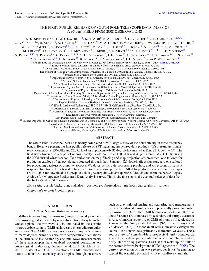
A thorough understanding of the detector beams, or angularresponse functions, is critical for interpreting the signals in SPTmaps. Sky signals are convolved with these functions in theprocess of observation, leading to the extended appearance ofpoint sources in the maps and the suppression of small-scalepower in the angular power spectrum. The structure of the SPTbeams can be characterized as a Gaussian main lobe out toa radius of 1 arcmin, near sidelobes at radii between 1 and5 arcmin, and a diffuse, low-level sidelobe at radii between 5and 40 arcmin relative to the beam center.
Dedicated observations of planets are valuable for measuringthe far sidelobes, since planets are bright enough to adequatelyprobe the tails of the response function. Planet observationsare less useful for studying the main beam, however, becauseof the limited dynamic range of the detectors, and because
the planets are extended sources. We use observations of thebrightest quasar in each survey field to characterize the mainbeam shape. We reconstruct a two-dimensional profile of thebeam by stitching together measurements of the “inner beam”within a 4 arcmin radius, and an “outer beam” covering radiifrom 4 arcmin to 40 arcmin.
The outer-beam measurements are based on seven dedicatedobservations of Venus performed in 2008 March, and onededicated observation of Jupiter performed in 2008 August.The observations consisted of a sequence of azimuth scans with0.5 arcmin elevation steps between scans. Because the detectorsare saturated when they observe the planets directly (and requireseveral detector time constants to recover), only data fromthe first half of each scan is used. For Jupiter observations,the impact of the Jovian satellites, which is very small tobegin with, is mitigated by subtracting a template based ontheir known locations. The Venus and Jupiter data are filteredto remove atmospheric noise and CMB fluctuations, with thelocations of the planets masked in the filtering. The averagescan-synchronous signal, as measured at distances larger than40 arcmin from the planet, is subtracted from the maps.
The inner beam shapes for this data release are measuredusing a bright quasar that appears in the ra5h30dec-55 fielditself and a bright quasar that appears in the other field observedby SPT in 2008, the ra23h30dec-55 field. We have no evidencethat the beam shape differs between these two fields. A smallmap is constructed around the brightest source in each field. Thesource is masked to a radius of 5 arcmin and filtering is appliedto remove atmospheric noise and CMB. The residual CMBand noise in the central beam region leads to an approximatelyconstant offset to the absolute response in this map. The innerbeam profile based on the quasar map is then stitched togetherwith the outer beam profile from Jupiter, with an iterativeprocedure that uses the Venus maps to determine the scalingbetween the two components and to correct for the constantoffset in the inner maps.
This procedure leads to a composite two-dimensional beamprofile that describes both the main beam and far-sideloberesponse of the instrument. In addition, because the inner-beam measurement is based on the final co-added maps ofthe fields, it encapsulates the contribution of several-arcsecondrandom pointing variations to the effective angular response inthe final maps. Pointing variations increase the effective beamwidth by approximately 3% and 5% at 150 GHz and 220 GHz,respectively.
The inner and outer beam profiles for both bands are presentedin Figure 1. The composite beam maps are available fordownload, as described in Section 7.
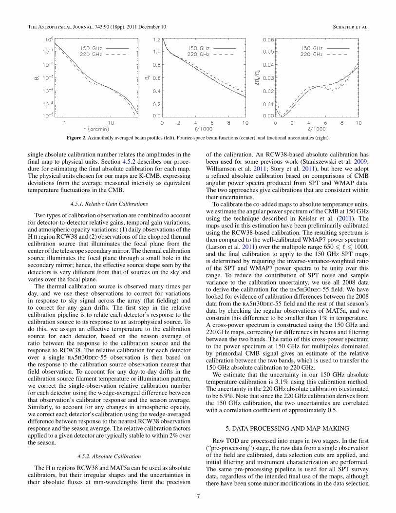
In many applications, it is preferable to use a simplifiedapproximation to the beam profiles rather than the full two-dimensional angular response functions. Azimuthally averagedbeam functions in map space and Fourier space are presentedin Figure 2. Using the flat-sky approximation, we calculate theFourier transform (FT) of the composite beam map, B(�, φ�).From this, we compute the azimuthally averaged beam function,
B� =√
1
2π
∫|B(�, φ�)|2 dφ�. (5)
There is a small bias (<0.5% fractional error at � < 10,000) inthis estimate of B� due to residual map noise and we removethis bias.
5
The Astrophysical Journal, 743:90 (18pp), 2011 December 10 Schaffer et al.
(a) 150 GHz inner beam (b) 220 GHz inner beam
(c) 150 GHz outer beam (d) 220 GHz outer beam
Figure 1. Two-dimensional average beam functions for the ra5h30dec-55 field. Panels (a) and (b) show the 150 GHz and 220 GHz two-dimensional beam profiles ona linear scale, emphasizing the structure of the “inner beam.” Panels (c) and (d) show the beam functions on a logarithmic scale out to much greater radii, emphasizingthe structure of the “outer beam,” and showing the stitching of the two beam estimates at a radius of 4 arcmin. Note that in panels (c) and (d) the absolute value hasbeen taken in order to display the image on a logarithmic scale, but this visually exaggerates the appearance of the noise in the innermost 4 arcmin of the beam.
The normalization of B(�) is somewhat arbitrary, in that itis degenerate with the absolute, CMB-power-spectrum-basedcalibration factor described in Section 4.5.2. Our CMB-power-spectrum-based calibration uses the multipole range 650 �� � 1000, so we choose to normalize B(�) to 1 at � = 800to minimize the correlation between beam uncertainty andcalibration uncertainty.
The uncertainty in our estimate of B(�) arises from severalstatistical and systematic effects, including residual atmosphericnoise in the maps of Venus and Jupiter, and the weak dependenceof B� on the choice of radius used to stitch together the innerand outer beam maps. We consider seven sources of uncertaintyin total. In Figure 2, we show the quadrature sum of these
error estimates, which approximates the total uncertainty. Thebeam functions are uncertain at the few percent level, and thisuncertainty increases mildly with increasing multipole number.
4.5. Calibration
Averaging measurements from many detectors within a givenobservation requires correcting for their relative gains. To aver-age multiple single-observation maps together, we also needto correct for inter-observation detector gain variations andchanges in atmospheric opacity that affect the calibration ofthe whole array. Section 4.5.1 describes our procedure for es-timating detector-to-detector and day-to-day relative calibra-tions. When all of these relative calibration factors are applied, a
6
The Astrophysical Journal, 743:90 (18pp), 2011 December 10 Schaffer et al.
Figure 2. Azimuthally averaged beam profiles (left), Fourier-space beam functions (center), and fractional uncertainties (right).
single absolute calibration number relates the amplitudes in thefinal map to physical units. Section 4.5.2 describes our proce-dure for estimating the final absolute calibration for each map.The physical units chosen for our maps are K-CMB, expressingdeviations from the average measured intensity as equivalenttemperature fluctuations in the CMB.
4.5.1. Relative Gain Calibrations
Two types of calibration observation are combined to accountfor detector-to-detector relative gains, temporal gain variations,and atmospheric opacity variations: (1) daily observations of theH ii region RCW38 and (2) observations of the chopped thermalcalibration source that illuminates the focal plane from thecenter of the telescope secondary mirror. The thermal calibrationsource illuminates the focal plane through a small hole in thesecondary mirror; hence, the effective source shape seen by thedetectors is very different from that of sources on the sky andvaries over the focal plane.
The thermal calibration source is observed many times perday, and we use these observations to correct for variationsin response to sky signal across the array (flat fielding) andto correct for any gain drifts. The first step in the relativecalibration pipeline is to relate each detector’s response to thecalibration source to its response to an astrophysical source. Todo this, we assign an effective temperature to the calibrationsource for each detector, based on the season average ofratio between the response to the calibration source and theresponse to RCW38. The relative calibration for each detectorover a single ra5h30dec-55 observation is then based onthe response to the calibration source observation nearest thatfield observation. To account for any day-to-day drifts in thecalibration source filament temperature or illumination pattern,we correct the single-observation relative calibration numberfor each detector using the wedge-averaged difference betweenthat observation’s calibrator response and the season average.Similarly, to account for any changes in atmospheric opacity,we correct each detector’s calibration using the wedge-averageddifference between response to the nearest RCW38 observationresponse and the season average. The relative calibration factorsapplied to a given detector are typically stable to within 2% overthe season.
4.5.2. Absolute Calibration
The H ii regions RCW38 and MAT5a can be used as absolutecalibrators, but their irregular shapes and the uncertainties intheir absolute fluxes at mm-wavelengths limit the precision
of the calibration. An RCW38-based absolute calibration hasbeen used for some previous work (Staniszewski et al. 2009;Williamson et al. 2011; Story et al. 2011), but here we adopta refined absolute calibration based on comparisons of CMBangular power spectra produced from SPT and WMAP data.The two approaches give calibrations that are consistent withintheir uncertainties.
To calibrate the co-added maps to absolute temperature units,we estimate the angular power spectrum of the CMB at 150 GHzusing the technique described in Keisler et al. (2011). Themaps used in this estimation have been preliminarily calibratedusing the RCW38-based calibration. The resulting spectrum isthen compared to the well-calibrated WMAP7 power spectrum(Larson et al. 2011) over the multipole range 650 � � � 1000,and the final calibration to apply to the 150 GHz SPT mapsis determined by requiring the inverse-variance-weighted ratioof the SPT and WMAP7 power spectra to be unity over thisrange. To reduce the contribution of SPT noise and samplevariance to the calibration uncertainty, we use all 2008 datato derive the calibration for the ra5h30dec-55 field. We havelooked for evidence of calibration differences between the 2008data from the ra5h30dec-55 field and the rest of that season’sdata by checking the regular observations of MAT5a, and weconstrain this difference to be smaller than 1% in temperature.A cross-power spectrum is constructed using the 150 GHz and220 GHz maps, correcting for differences in beams and filteringbetween the two bands. The ratio of this cross-power spectrumto the power spectrum at 150 GHz for multipoles dominatedby primordial CMB signal gives an estimate of the relativecalibration between the two bands, which is used to transfer the150 GHz absolute calibration to 220 GHz.
We estimate that the uncertainty in our 150 GHz absolutetemperature calibration is 3.1% using this calibration method.The uncertainty in the 220 GHz absolute calibration is estimatedto be 6.9%. Note that since the 220 GHz calibration derives fromthe 150 GHz calibration, the two uncertainties are correlatedwith a correlation coefficient of approximately 0.5.
5. DATA PROCESSING AND MAP-MAKING
Raw TOD are processed into maps in two stages. In the first(“pre-processing”) stage, the raw data from a single observationof the field are calibrated, data selection cuts are applied, andinitial filtering and instrument characterization are performed.The same pre-processing pipeline is used for all SPT surveydata, regardless of the intended final use of the maps, althoughthere have been some minor modifications in the data selection
7
The Astrophysical Journal, 743:90 (18pp), 2011 December 10 Schaffer et al.
criteria and pre-processing algorithms over the history of SPTdata analysis.
In the second (“map-making”) stage, additional filtering isperformed on the pre-processed TOD and the data are binnedinto single-observation maps used for final co-adds. The filteringapplied in the map-making stage is typically customized fordifferent analyses, as is the choice of map projection. Asdescribed in detail below, we present two specific combinationsof filtering and map projection in this release.
We characterize the effect of the filtering and projectionchoices by describing the Fourier-space properties of the maps.We refer to features in the Fourier plane using the correspondingangular wavenumbers in radians k. The maps are oriented suchthat at the center of the map, the x-direction corresponds to R.A.and the y-direction corresponds to declination.
5.1. Data Selection and Pre-processing
The first steps in the pre-processing pipeline are to character-ize detector performance, assemble measured response charac-teristics, and calculate calibration factors and weights.
Summary statistics are first calculated to characterize thereceiver setup and the TOD for each detector. Each detector’sTOD for an entire 2 hr observation is used to estimate the powerspectral density (PSD) for that detector. A fit to the noise PSDis then used to identify line-like features that deviate from a 1/fplus white noise profile. Additional noise statistics are calculatedfor the SQUIDs.
Next, a set of responsivity statistics is assembled for everydetector. These include the amplitude of the detector’s responseto the chopped thermal calibrator, the amplitude of its responseduring a calibration observation of RCW38, and the amplitudeof its response to a two-degree elevation scan performedbefore each field observation. These response parameters areused to calculate daily gain calibrations for each detector, aspreviously described in Section 4.5. They are also used to definedata selection cuts.
Preliminary cuts verify that each bolometer’s bias voltage andreadout configuration settings are within the nominal ranges andthat the TOD values for each channel remain within the dynamicrange of the digitizer. Once these initial cuts have been applied,bad bolometers are rejected with progressively more and morestringent assessments of responsivity and noise.
The first such cuts enforce a minimum signal-to-noise re-sponse to the chopped calibration source and a minimum re-sponse to the routine elevation scans. Bolometers are alsorejected if their response to the elevation scans does not fit theexpected modulation of the atmosphere. If a detector’s responseto the chopped calibration source or the short elevation scansis more than three standard deviations away from the medianresponse for detectors of the same band, it is also rejected. De-tectors are rejected if their PSDs exhibit wide line-like featuresor too many lines. After all of these cuts are applied, a final pairof cuts rejects bolometers with calibration constants or noiseweights that deviate by more than a factor of three from themedian for each band. The median numbers of detectors thatpass cuts for the ra5h30dec-55 field observations (quoted inSection 5.6) reflect the bolometers selected through this process.
The bolometer data are parsed into scans, defined as tempo-rally contiguous periods of constant-velocity azimuth scanningin either direction across the field. Cutting periods of time whenthe telescope is accelerating (at the ends of each scan) removesabout 5% of the total TOD for an observation. All data for a givenscan are cut if the receiver temperature exceeded the nominal
operating value at any time during the scan, if the telescope fol-lowing error (absolute value of the commanded position minusthe position recorded by the encoders) exceeded 20′′ at any timeduring the scan, or if there were data acquisition problems lead-ing to bolometer data or pointing data drop-outs during the scan.Typically about 5% of scans are cut for these reasons. Data foran individual bolometer in an individual scan are also rejectedif that bolometer shows evidence of step-function features inits TOD (which can sometimes occur due to “flux jumps” inthe SQUIDs), if the SQUID or bolometer noise for that scan isexcessive, or if any of the digitized SQUID data approach thelimits of the dynamic range. A spike-finding algorithm identi-fies cosmic-ray-like events in the TODs for individual detectors.If there are fewer than five in a given scan, and the spike fea-tures are relatively small, we remove them and interpolate overthe gaps; otherwise, we flag and ignore affected TODs for theduration of the scan. Typically, around 5% of otherwise well-performing bolometers are cut from each scan for any of thesereasons.
Because a varying subset of detectors will sometimes showsensitivity to the receiver’s pulse-tube cooler (a phenomenonalso seen in other TES bolometer systems with pulse-tubecoolers, e.g., Dicker et al. 2009), we apply a notch filter toremove a small amount of bandwidth from all data during thepre-processing stage. Combining all data that pass selection cutsfor a given observation, we identify the fundamental frequencyof the pulse-tube cooler and notch-filter a conservative 0.007 Hzof bandwidth around this frequency as well as any strongharmonics. For the 2008 ra5h30dec-55 field observations, thepulse tube operating frequency was 1.62 Hz. If all harmonics ofthis frequency were always cut, this would represent an absolutemaximum of 0.4% of the total bandwidth; the actual bandwidthcut is smaller since typically only the first few harmonics arecut. We have verified that this notch filter has a negligible effecton further analysis, and we neglect it in further analysis steps.
After all pre-processing, the offline pointing model is usedto calculate corrected pointing positions to associate with everytime sample, and the pre-processed data are written into anintermediate data format for further analysis.
5.2. Filtering
After the pre-processing stage of data analysis, the TOD as-sociated with a given field observation is further filtered ona scan-by-scan basis. The processing of each scan (1) decon-volves the detector temporal response functions, (2) removeshigh-frequency temporal noise that translates to spatial scalessmaller than the pixel resolution in the maps, and (3) removes at-mospheric noise while minimizing the filtering of signal power.
The time-constant deconvolution and low-pass anti-aliasingfilters are applied in a single Fourier-domain operation on eachscan for each detector. The time-constant deconvolution takesinto account the measured time constants for every individualdetector (see Section 4.2). A cutoff frequency of 25 Hz is usedfor the low-pass filter applied to the TOD, chosen to limit noiseon spatial scales smaller than the 0.25 arcmin map pixels withoutsuppressing power on the spatial scales of the SPT beams.
Prior to averaging the data into maps, additional time-domain filtering is applied to remove atmospheric noise. Theatmospheric contamination resides primarily at low temporalfrequencies, so a high-pass filter is an effective way to removethe most contaminated data. However, the application of aFourier-domain high-pass filter will also distort the appearanceof bright point sources in the final maps, introducing “ringing”
8
The Astrophysical Journal, 743:90 (18pp), 2011 December 10 Schaffer et al.
patterns. This effect can be avoided by filtering in the timedomain via fitting to slowly varying template functions andmasking the locations of known bright point sources during thefit. Point-source masking of this sort has been performed forone of the sets of maps in this release, but not for the other, asexplained in Section 5.3.
In all variations of our analysis, we fit out a mean and slope aswell as higher-order polynomials from each scan. In some pastwork we have subtracted Legendre polynomials and in others aseries of sines and cosines (Fourier modes). In either case theresult is a time-domain high-pass filter that allows for point-source masking as needed. For the maps in this release, we havefit Fourier modes up to a temporal frequency that correspondsto a spatial high-pass cutoff of k = 300 in the scan direction,or kx = 300 (because the scan direction corresponds to thex-direction in our maps).
Atmospheric noise is highly correlated across the detectorarray. By taking this correlation into account, we can filteradditional atmospheric noise without affecting small-scale skysignal. For each TOD sample, we subtract the mean value acrossevery detector in a given wedge. This filter can also be performedwith the locations of bright point sources masked, and thismasking is performed in one set of maps in this release (aswith the masking in the time-series filters).
5.3. Filtering Variations for Maps in This Release
This paper presents two sets of maps, one tailored to clusteranalysis and one tailored to point-source analysis.26 For clusteranalysis, the point sources in the maps are viewed as a fore-ground. The locations of known point sources are masked in thefiltering for these maps in order to prevent artifacts from ringing,which could affect cluster extraction. The brightest 201 sourcesare masked in the filtering, with the top 9 masked to a radiusof 5 arcmin and the rest masked to 2 arcmin. The source listused for constructing the mask was created by merging togetherall sources detected at greater than 5σ significance in either150 GHz or 220 GHz maps, from the published point-sourcecatalog for this field (Vieira et al. 2010), and adding any sourcesthat lie outside the field boundaries used for detection in thatwork but that are strongly detected in an analysis using all mappixels.
When the point sources themselves are the object of study,it is preferable to filter them in the same way as the otherparts of the map, so that the effect of filtering on signal can becompletely characterized. For the set of maps tailored to point-source analysis, the brightest point sources are not masked inthe filtering. We also choose different map projections for thetwo sets of maps, as described below. All other parameters ofthe data processing and filtering are equivalent in both sets ofmaps.
5.4. Map Projections
After all data selection and filtering has been performed, weuse the corrected pointing information to average and bin thedata into pixels in a two-dimensional map. For small areas ofthe sky, analysis of the maps is greatly simplified by using aflat-sky approximation. This allows two-dimensional FTs to beused (rather than spherical harmonic transforms) for analyzingsignal power, noise, and instrument response as a function of
26 The majority of extragalactic emissive sources appear point like in thearcminute-resolution SPT maps, and we use “point source” and “emissivesource” interchangeably in this work.
angular scale. However, any choice of map projection will leadto some distortions of information in the map. The characterof these distortions varies depending on the selected projection,meaning that some analyses may be easier to perform on mapswith one projection while others may be easier with another.
In past work we have employed several different projectionschemes, of which two have been selected for presentation here.Past SPT cluster-finding analysis has used the Sanson-Flamsteedprojection (e.g., Calabretta & Greisen 2002), which projectsconstant-elevation scans into pixel rows in the final map. Thisprojection choice simplifies the characterization and treatmentof signal filtering, because the TOD processing effectivelyoperates on map rows. The disadvantage of this projection is thatit is not distance preserving, and sky features near the cornersof the maps will therefore have slightly distorted shapes (forexample, a 1 arcmin circle will appear to have an ellipticity ofε ∼ 0.12 near the corner of the ra5h30dec-55 map). We haveselected this projection for the maps tailored to cluster finding.
The second projection employed here, for the maps tailoredto point-source analysis, is the oblique Lambert equal-area az-imuthal projection. For the typical size, shape, and center loca-tion of SPT maps, this sky projection preserves both distancesand areas to high accuracy (Snyder 1987), which means thatthe effective beam shape will not vary significantly for differentlocations in the map. This is particularly advantageous for recon-structing point-source amplitudes using variants of the CLEANalgorithm (Hogbom 1974). The disadvantage of this projectionis that the effective filtering has a strong position dependence,since the angle between the scan direction and the map pixelrows changes across the map. For constant-declination scans,this angle, α, can be expressed as
α = tan−1(A/B), (6)
where
A = γ sin θ0 sin(φ0 − φ)
× (sin θ0 cos θ + sin θ cos θ0 cos(φ0 − φ))
+ cos θ0 sin(φ0 − φ),
B = γ sin θ0 sin2(φ0 − φ) sin θ + cos(φ0 − φ),
and
γ = 0.5
1 + cos θ0 cos θ + sin θ0 sin θ cos(φ0 − φ).
Here φ equals the R.A. in radians, while θ = π/2−declination,also in radians. Unsubscripted variables represent the pixellocation and the subscript “0” denotes the field center.
In Sections 6.2 and 6.3, we will discuss the impact of thechoice of projection on the signal and noise properties in thesemaps.
5.5. Weights
The weights used to co-add data from many detectors intoa single-observation map are calculated by averaging the cal-ibrated PSD for each detector between 1 and 3 Hz. For thetelescope scan speeds used in observations of the ra5h30dec-55 field, this frequency range corresponds to a multipole rangeof roughly 1500 < � < 4500 in the scan direction, a reason-able overlap with the scales of interest for source and clusterdetection and for high-� power spectrum analyses.
9
The Astrophysical Journal, 743:90 (18pp), 2011 December 10 Schaffer et al.
When we average the data from individual detectors to obtaina measurement of the map value in a particular pixel, wecalculate the total weight for that pixel by combining the weightsfrom each individual detector. These pixel weights are usedto combine the multiple single-observation maps into a finalco-added map (see Section 5.6). The primary source of noisevariation between single-observation maps is the weather, whichis accurately reflected in the calibrated 1–3 Hz noise estimatesfor the individual detectors in all but the poorest-weather days.
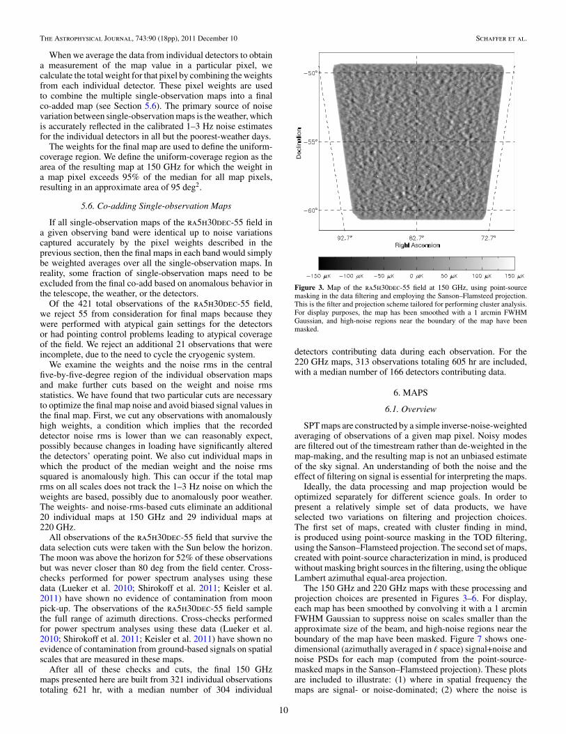
The weights for the final map are used to define the uniform-coverage region. We define the uniform-coverage region as thearea of the resulting map at 150 GHz for which the weight ina map pixel exceeds 95% of the median for all map pixels,resulting in an approximate area of 95 deg2.
5.6. Co-adding Single-observation Maps
If all single-observation maps of the ra5h30dec-55 field ina given observing band were identical up to noise variationscaptured accurately by the pixel weights described in theprevious section, then the final maps in each band would simplybe weighted averages over all the single-observation maps. Inreality, some fraction of single-observation maps need to beexcluded from the final co-add based on anomalous behavior inthe telescope, the weather, or the detectors.
Of the 421 total observations of the ra5h30dec-55 field,we reject 55 from consideration for final maps because theywere performed with atypical gain settings for the detectorsor had pointing control problems leading to atypical coverageof the field. We reject an additional 21 observations that wereincomplete, due to the need to cycle the cryogenic system.
We examine the weights and the noise rms in the centralfive-by-five-degree region of the individual observation mapsand make further cuts based on the weight and noise rmsstatistics. We have found that two particular cuts are necessaryto optimize the final map noise and avoid biased signal values inthe final map. First, we cut any observations with anomalouslyhigh weights, a condition which implies that the recordeddetector noise rms is lower than we can reasonably expect,possibly because changes in loading have significantly alteredthe detectors’ operating point. We also cut individual maps inwhich the product of the median weight and the noise rmssquared is anomalously high. This can occur if the total maprms on all scales does not track the 1–3 Hz noise on which theweights are based, possibly due to anomalously poor weather.The weights- and noise-rms-based cuts eliminate an additional20 individual maps at 150 GHz and 29 individual maps at220 GHz.
All observations of the ra5h30dec-55 field that survive thedata selection cuts were taken with the Sun below the horizon.The moon was above the horizon for 52% of these observationsbut was never closer than 80 deg from the field center. Cross-checks performed for power spectrum analyses using thesedata (Lueker et al. 2010; Shirokoff et al. 2011; Keisler et al.2011) have shown no evidence of contamination from moonpick-up. The observations of the ra5h30dec-55 field samplethe full range of azimuth directions. Cross-checks performedfor power spectrum analyses using these data (Lueker et al.2010; Shirokoff et al. 2011; Keisler et al. 2011) have shown noevidence of contamination from ground-based signals on spatialscales that are measured in these maps.
After all of these checks and cuts, the final 150 GHzmaps presented here are built from 321 individual observationstotaling 621 hr, with a median number of 304 individual
Figure 3. Map of the ra5h30dec-55 field at 150 GHz, using point-sourcemasking in the data filtering and employing the Sanson–Flamsteed projection.This is the filter and projection scheme tailored for performing cluster analysis.For display purposes, the map has been smoothed with a 1 arcmin FWHMGaussian, and high-noise regions near the boundary of the map have beenmasked.
detectors contributing data during each observation. For the220 GHz maps, 313 observations totaling 605 hr are included,with a median number of 166 detectors contributing data.
6. MAPS
6.1. Overview
SPT maps are constructed by a simple inverse-noise-weightedaveraging of observations of a given map pixel. Noisy modesare filtered out of the timestream rather than de-weighted in themap-making, and the resulting map is not an unbiased estimateof the sky signal. An understanding of both the noise and theeffect of filtering on signal is essential for interpreting the maps.
Ideally, the data processing and map projection would beoptimized separately for different science goals. In order topresent a relatively simple set of data products, we haveselected two variations on filtering and projection choices.The first set of maps, created with cluster finding in mind,is produced using point-source masking in the TOD filtering,using the Sanson–Flamsteed projection. The second set of maps,created with point-source characterization in mind, is producedwithout masking bright sources in the filtering, using the obliqueLambert azimuthal equal-area projection.
The 150 GHz and 220 GHz maps with these processing andprojection choices are presented in Figures 3–6. For display,each map has been smoothed by convolving it with a 1 arcminFWHM Gaussian to suppress noise on scales smaller than theapproximate size of the beam, and high-noise regions near theboundary of the map have been masked. Figure 7 shows one-dimensional (azimuthally averaged in � space) signal+noise andnoise PSDs for each map (computed from the point-source-masked maps in the Sanson–Flamsteed projection). These plotsare included to illustrate: (1) where in spatial frequency themaps are signal- or noise-dominated; (2) where the noise is
10
The Astrophysical Journal, 743:90 (18pp), 2011 December 10 Schaffer et al.
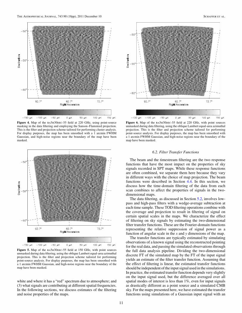
Figure 4. Map of the ra5h30dec-55 field at 220 GHz, using point-sourcemasking in the data filtering and employing the Sanson–Flamsteed projection.This is the filter and projection scheme tailored for performing cluster analysis.For display purposes, the map has been smoothed with a 1 arcmin FWHMGaussian, and high-noise regions near the boundary of the map have beenmasked.
Figure 5. Map of the ra5h30dec-55 field at 150 GHz, with point sourcesunmasked during data filtering, using the oblique Lambert equal-area azimuthalprojection. This is the filter and projection scheme tailored for performingpoint-source analysis. For display purposes, the map has been smoothed witha 1 arcmin FWHM Gaussian, and high-noise regions near the boundary of themap have been masked.
white and where it has a “red” spectrum due to atmosphere; and(3) what signals are contributing at different spatial frequencies.In the following sections, we discuss estimates of the filteringand noise properties of the maps.
Figure 6. Map of the ra5h30dec-55 field at 220 GHz, with point sourcesunmasked during data filtering, using the oblique Lambert equal-area azimuthalprojection. This is the filter and projection scheme tailored for performingpoint-source analysis. For display purposes, the map has been smoothed witha 1 arcmin FWHM Gaussian, and high-noise regions near the boundary of themap have been masked.
6.2. Filter Transfer Functions
The beam and the timestream filtering are the two responsefunctions that have the most impact on the properties of skysignals recorded in SPT maps. While these response functionsare often combined, we separate them here because they varyin different ways with the choice of map projection. The beamfunctions were described in Section 4.4. In this section, wediscuss how the time-domain filtering of the data from eachscan combines to affect the properties of signals in the two-dimensional maps.
The data filtering, as discussed in Section 5.2, involves low-pass and high-pass filters with a wedge-average subtraction ateach time sample. These TOD filtering operations combine withthe coverage and projection to result in filtering of signal oncertain spatial scales in the maps. We characterize the effectof filtering on sky signals by estimating the two-dimensionalfilter transfer functions. These are the Fourier-domain functionsrepresenting the relative suppression of signal power as afunction of angular scale in the x and y dimensions of the map.
The transfer functions are typically estimated by simulatingobservations of a known signal using the reconstructed pointingfor the real data, and passing the simulated observations throughthe full data analysis pipeline. Dividing the two-dimensionaldiscrete FT of the simulated map by the FT of the input signalyields an estimate of the filter transfer function. Assuming thatthe effect of filtering is linear, the estimated transfer functionsshould be independent of the input signal used in the simulations.In practice, the estimated transfer function depends very slightlyon the input signal used, but the difference averaged over allspatial modes of interest is less than 1%, even for input signalsas drastically different as a point source and a simulated CMBsky. For the maps presented here, we have estimated the transferfunctions using simulations of a Gaussian input signal with an
11
The Astrophysical Journal, 743:90 (18pp), 2011 December 10 Schaffer et al.
Figure 7. One-dimensional (azimuthally averaged in � space) signal+noise and noise PSDs for each observing frequency. Left panel: signal+noise and noise-onlyPSDs from the raw map, uncorrected for beam and filtering effects. Right panel: as in left panel, but with the beam and filter transfer function divided out. Azimuthalaverages are calculated using rough noise weighting, with noisier modes at low kx (or �x ) receiving less weight and modes below kx = �x = 400 ignored entirely.These demonstrate that the 150 GHz map is signal dominated at nearly all spatial frequencies out to � = 10,000, but that the 220 GHz map has significant noisecontributions, particularly at � � 5000. The essentially white character of the map noise is evident above � = 2000 in the raw map PSDs. The signal+noise PSDs withthe beam and transfer function divided out show that the damping tail of the primary CMB (steeply falling with �) dominates the signal below � 2500, while thecontribution from point sources (flat with �) dominates above � 2500.
(A color version of this figure is available in the online journal.)
(a) Filter transfer function for 150 GHz (b) Filter transfer function for 220 GHz
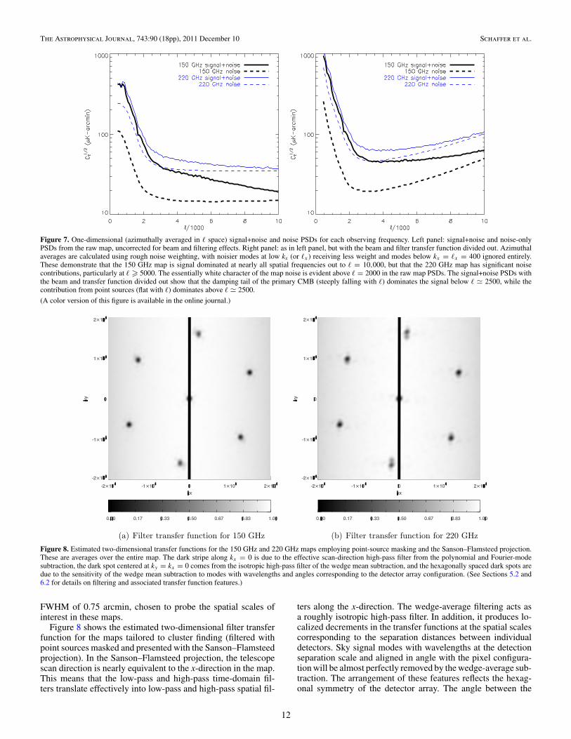
Figure 8. Estimated two-dimensional transfer functions for the 150 GHz and 220 GHz maps employing point-source masking and the Sanson–Flamsteed projection.These are averages over the entire map. The dark stripe along kx = 0 is due to the effective scan-direction high-pass filter from the polynomial and Fourier-modesubtraction, the dark spot centered at ky = kx = 0 comes from the isotropic high-pass filter of the wedge mean subtraction, and the hexagonally spaced dark spots aredue to the sensitivity of the wedge mean subtraction to modes with wavelengths and angles corresponding to the detector array configuration. (See Sections 5.2 and6.2 for details on filtering and associated transfer function features.)
FWHM of 0.75 arcmin, chosen to probe the spatial scales ofinterest in these maps.
Figure 8 shows the estimated two-dimensional filter transferfunction for the maps tailored to cluster finding (filtered withpoint sources masked and presented with the Sanson–Flamsteedprojection). In the Sanson–Flamsteed projection, the telescopescan direction is nearly equivalent to the x-direction in the map.This means that the low-pass and high-pass time-domain fil-ters translate effectively into low-pass and high-pass spatial fil-
ters along the x-direction. The wedge-average filtering acts asa roughly isotropic high-pass filter. In addition, it produces lo-calized decrements in the transfer functions at the spatial scalescorresponding to the separation distances between individualdetectors. Sky signal modes with wavelengths at the detectionseparation scale and aligned in angle with the pixel configura-tion will be almost perfectly removed by the wedge-average sub-traction. The arrangement of these features reflects the hexag-onal symmetry of the detector array. The angle between the
12
The Astrophysical Journal, 743:90 (18pp), 2011 December 10 Schaffer et al.
(a) Center filter transfer function for 150 GHz map (b) Corner filter transfer function for 150 GHz map
(c) Center filter transfer function for 220 GHz map (d) Corner filter transfer function for 220 GHz map
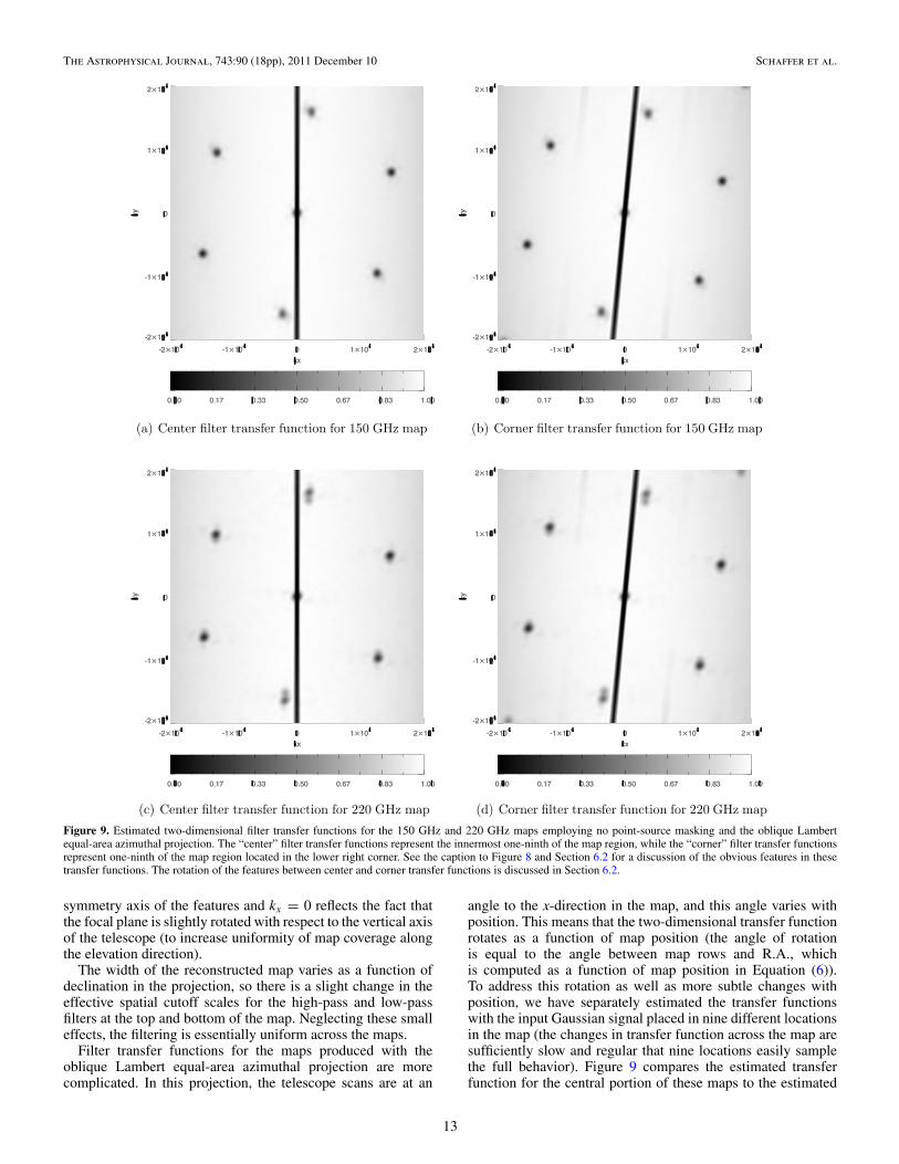
Figure 9. Estimated two-dimensional filter transfer functions for the 150 GHz and 220 GHz maps employing no point-source masking and the oblique Lambertequal-area azimuthal projection. The “center” filter transfer functions represent the innermost one-ninth of the map region, while the “corner” filter transfer functionsrepresent one-ninth of the map region located in the lower right corner. See the caption to Figure 8 and Section 6.2 for a discussion of the obvious features in thesetransfer functions. The rotation of the features between center and corner transfer functions is discussed in Section 6.2.
symmetry axis of the features and kx = 0 reflects the fact thatthe focal plane is slightly rotated with respect to the vertical axisof the telescope (to increase uniformity of map coverage alongthe elevation direction).
The width of the reconstructed map varies as a function ofdeclination in the projection, so there is a slight change in theeffective spatial cutoff scales for the high-pass and low-passfilters at the top and bottom of the map. Neglecting these smalleffects, the filtering is essentially uniform across the maps.
Filter transfer functions for the maps produced with theoblique Lambert equal-area azimuthal projection are morecomplicated. In this projection, the telescope scans are at an
angle to the x-direction in the map, and this angle varies withposition. This means that the two-dimensional transfer functionrotates as a function of map position (the angle of rotationis equal to the angle between map rows and R.A., whichis computed as a function of map position in Equation (6)).To address this rotation as well as more subtle changes withposition, we have separately estimated the transfer functionswith the input Gaussian signal placed in nine different locationsin the map (the changes in transfer function across the map aresufficiently slow and regular that nine locations easily samplethe full behavior). Figure 9 compares the estimated transferfunction for the central portion of these maps to the estimated
13
The Astrophysical Journal, 743:90 (18pp), 2011 December 10 Schaffer et al.
(a) Noise PSD for the 150 GHz map (b) Noise PSD for the 220 GHz map
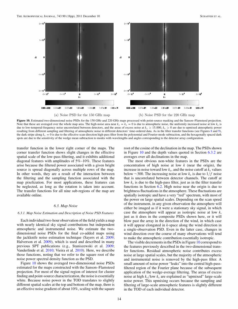
Figure 10. Estimated two-dimensional noise PSDs for the 150 GHz and 220 GHz maps processed with point-source masking and the Sanson–Flamsteed projection.Note that these are averaged over the whole map area. The high-noise area near ky = kx = 0 is due to atmospheric noise, the uniformly increased noise at low kx isdue to low-temporal-frequency noise uncorrelated between detectors, and the areas of excess noise at ky 15,000, kx 0 are due to upmixed atmospheric powerresulting from different sampling and filtering of atmospheric noise in different detectors’ time-ordered data. As in the filter transfer functions (see Figures 8 and 9),the dark stripe along kx = 0 is due to the effective scan-direction high-pass filter from the polynomial and Fourier-mode subtraction, and the hexagonally spaced darkspots are due to the sensitivity of the wedge mean subtraction to modes with wavelengths and angles corresponding to the detector array configuration.
transfer function in the lower right corner of the maps. Thecorner transfer function shows slight changes in the effectivespatial scale of the low-pass filtering, and it exhibits additionaldiagonal features with amplitudes of 5%–10%. These featuresarise because the filtered power associated with a given brightsource is spread diagonally across multiple rows of the map.In other words, they are a result of the interaction betweenthe filtering and the sampling function associated with themap pixelization. For most applications, these features canbe neglected, as long as the rotation is taken into account.The transfer functions for all nine sub-regions of the map areavailable online.
6.3. Map Noise
6.3.1. Map Noise Estimation and Description of Noise PSD Features
Each individual two-hour observation of the field yields a mapwith nearly identical sky signal contributions but independentatmospheric and instrumental noise. We estimate the two-dimensional noise PSDs for the final co-added maps usingthe jackknife noise estimation technique (Sayers et al. 2009;Halverson et al. 2009), which is used and described in manyprevious SPT publications (e.g., Staniszewski et al. 2009;Vanderlinde et al. 2010; Vieira et al. 2010). Here, we describethose functions, noting that we refer to the square root of thenoise power spectral density function as the PSD.
Figure 10 shows the averaged two-dimensional noise PSDsestimated for the maps constructed with the Sanson–Flamsteedprojection. For most of the signal region of interest for clusterfinding and point-source characterization, the noise is essentiallywhite. Because noise power in the TOD translates to slightlydifferent spatial scales at the top and bottom of the map, there isan effective noise gradient of about 10%, scaling with the square
root of the cosine of the declination in the map. The PSDs shownin Figure 10 and the depth values quoted in Section 6.3.2 areaverages over all declinations in the map.
The most obvious non-white features in the PSDs are theconcentration of high noise at low k (near the origin), theincrease in noise toward low kx, and the noise cutoff at kx valuesbelow ∼300. The increasing noise at low kx is due to 1/f noisethat is uncorrelated between detector channels. The cutoff atlow kx is due to the high-pass filter, just as in the filter transferfunctions in Section 6.2. High noise near the origin is due tobrightness fluctuations in the atmosphere. These fluctuations arespatially isotropic and have a very “red” spectrum, with most ofthe power on large spatial scales. Depending on the scan speedof the instrument, in any given observation the atmosphere willeither be imaged as if it were a stationary sky signal, in whichcase the atmosphere will appear as isotropic noise at low k,just as it does in the composite PSDs shown here, or it willblow past the array in the direction of the wind, in which caseit will appear elongated in k-space along the wind direction ina single-observation PSD. Even in the latter case, changes inwind direction over the course of many observations will tendto make the atmospheric contribution essentially isotropic.
The visible decrements in the PSDs in Figure 10 correspond tothe features previously described in the two-dimensional trans-fer functions. Residual atmospheric noise contributes excessnoise at large spatial scales, but the majority of the atmosphericand instrumental noise is removed by the high-pass filter. Asmall amount of noise power “leaks” into the central high-pass-filtered region of the Fourier plane because of the subsequentapplication of the wedge-average filtering. The areas of excessnoise at high ky/low kx are explained as “upmixed” large-scalenoise power. This upmixing occurs because the sampling andfiltering of large-scale atmospheric features is slightly differentin the TOD of each individual detector.
14

The Astrophysical Journal, 743:90 (18pp), 2011 December 10 Schaffer et al.
(a) Center noise PSD for the 150 GHz map (b) Corner noise PSD for the 150 GHz map
(c) Center noise PSD for the 220 GHz map (d) Corner noise PSD for the 220 GHz map
Figure 11. Estimated two-dimensional noise PSDs for selected sub-regions of the 150 GHz and 220 GHz maps processed with no point-source masking and the obliqueLambert equal-area azimuthal projection. The “center” PSDs represent the innermost one-ninth of the map region, while the “corner” PSDs represent one-ninth of themap region located in the lower right corner. See the caption to Figure 10 and Section 6.3.1 for a discussion of the obvious features in these PSDs. The faint lines atconstant kx (not apparent in the Figure 10 PSDs) are due to readout lines (see Section 6.3.1 for details). The rotation of the features between center and corner PSDs isdiscussed in Section 6.3.1.
Figure 11 shows the averaged two-dimensional noise PSDsestimated for the center and lower right corner of the mapswith the oblique Lambert equal-area azimuthal projection.The properties are similar to those for the Sanson–Flamsteedprojection, with the added rotation for positions away from thecenter of the map (the reason for this rotation and the value ofthe rotation angle are identical to those discussed for the filtertransfer functions in Section 6.2). In these PSDs, the effect ofresidual high-frequency readout-related line features is visibleas vertical strips at high kx. These are less visible in the full-map average PSDs presented in Figure 10, but the features are
present. These features have a negligible effect on analysesperformed with the maps.
As with the transfer functions, PSDs have been estimated fornine sub-regions of the oblique Lambert equal-area azimuthalprojection maps, and these data products are available todownload.
6.3.2. Map Noise Accounting
The noise PSDs discussed in Section 6.3.1 can be used to es-timate the effective map depths, but it is important to highlightthat these numbers depend on the absolute calibration and on
15
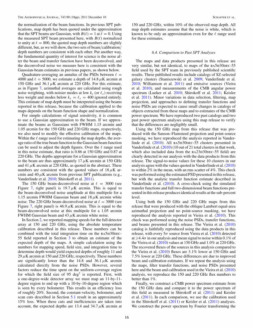
The Astrophysical Journal, 743:90 (18pp), 2011 December 10 Schaffer et al.
the normalization of the beam functions. In previous SPT pub-lications, map depth has been quoted under the approximationthat the SPT beams are Gaussian, with B(�) = 1 at � = 0. Usingthe measured SPT beam presented here, with B(�) normalizedto unity at � = 800, the quoted map depth numbers are slightlydifferent, but, as we will show, the two sets of beam/calibration/depth numbers are consistent with each other. Put another way,the fundamental quantity of interest for science is the noise af-ter the beam and transfer function have been deconvolved, andthe deconvolved noise we measure here is consistent with theGaussian-beam estimates in previous papers, as shown below.
Quadrature-averaging an annulus of the PSDs between � =4000 and � = 5000, we estimate a depth of 14.8 μK arcmin at150 GHz and 36.1 μK arcmin at 220 GHz. For this estimate,as in Figure 7, azimuthal averages are calculated using roughnoise weighting, with noisier modes at low kx (or �x) receivingless weight and modes below kx = �x = 400 ignored entirely.This estimate of map depth must be interpreted using the beamsreported in this release, because the calibration applied to themaps depends on the beam function shape and normalization.
For simple calculations of signal sensitivity, it is commonto use a Gaussian approximation to the beam. If we approx-imate the beams as Gaussians with FWHM 1.15 arcmin and1.05 arcmin for the 150 GHz and 220 GHz maps, respectively,we also need to modify the effective calibration of the maps.Within the � range used for estimating the map depths, the aver-age ratio of the true beam function to the Gaussian beam functioncan be used to adjust the depth figures. Over the � range usedin this noise estimate, that ratio is 0.86 at 150 GHz and 0.87 at220 GHz. The depths appropriate for a Gaussian approximationto the beam are thus approximately 17 μK arcmin at 150 GHzand 41 μK arcmin at 220 GHz, as quoted in the abstract. Thesenumbers are consistent with the quoted values of 18 μK ar-cmin and 40 μK arcmin from previous SPT publications (e.g.,Vanderlinde et al. 2010; Shirokoff et al. 2011).
The 150 GHz beam-deconvolved noise at � = 3000 (seeFigure 7, right panel) is 19.7 μK arcmin. This is equal tothe beam-deconvolved noise amplitude at this multipole for a1.15 arcmin FWHM Gaussian beam and 18 μK arcmin whitenoise. The 220 GHz beam-deconvolved noise at � = 3000 (seeFigure 7, right panel) is 46.9 μK arcmin. This is equal to thebeam-deconvolved noise at this multipole for a 1.05 arcminFWHM Gaussian beam and 43 μK arcmin white noise.
In Section 2, we reported mapping speeds for the full detectorarray at 150 and 220 GHz, using the absolute temperaturecalibration described in this release. These numbers can becombined with the total integration time on the ra5h30dec-55 field reported in Section 3 to obtain an estimate of theexpected depth of the maps. A simple calculation using thenumbers for mapping speed, field size, and integration time todetermine depth would yield expected depths of roughly 11 and29 μK arcmin at 150 and 220 GHz, respectively. These numbersare significantly lower than the 14.8 and 36.1 μK arcmincalculated directly from the noise PSDs. However, severalfactors reduce the time spent on the uniform-coverage regionfor which the field size of 95 deg2 is reported. First, witha one-degree-wide detector array we must map an 11-by-11-degree region to end up with a 10-by-10-degree region whichis seen by every bolometer. This results in an efficiency lossof roughly 20%. Second, the constant-velocity, bolometer, andscan cuts described in Section 5.1 result in an approximately15% loss. When these cuts and inefficiencies are taken intoaccount, the expected depths are 13.4 and 34.7 μK arcmin at
150 and 220 GHz, within 10% of the observed map depth. Allmap depth estimates assume that the noise is white, which isknown to be only an approximation even for the � range usedfor these estimates.
6.4. Comparison to Past SPT Analyses
The maps and data products presented in this release arevery similar, but not identical, to maps of the ra5h30dec-55field used by the SPT team in previously published scientificresults. These published results include catalogs of SZ-selectedgalaxy clusters (Staniszewski et al. 2009; Vanderlinde et al.2010; Williamson et al. 2011) and emissive sources (Vieiraet al. 2010), and measurements of the CMB angular powerspectrum (Lueker et al. 2010; Shirokoff et al. 2011; Keisleret al. 2011). Minor variations in data selection, filtering, mapprojection, and approaches to defining transfer functions andnoise PSDs are expected to cause small changes in catalogs ofobjects extracted from these maps and to estimates of the CMBpower spectrum. We have reproduced two past catalogs and twopast power spectrum analyses using this map release to verifythat the differences are negligibly small.
Using the 150 GHz map from this release that was pro-duced with the Sanson–Flamsteed projection and point-sourcemasking, we have reproduced the analysis reported in Vander-linde et al. (2010). All ra5h30dec-55 clusters presented inVanderlinde et al. (2010) (10 out of 21 total clusters in that work,which also included data from the ra23h30dec-55 field) areclearly detected in our analysis with the data products from thisrelease. The signal-to-noise values for these 10 clusters in ouranalysis agree with the values quoted in Vanderlinde et al. (2010)to within 2% in the mean, with an rms scatter of 4%. This checkwas performed using the estimated PSD presented in this release,but with the analytic transfer function estimate described inVanderlinde et al. (2010). A cross-check using the simulatedtransfer functions and full two-dimensional beam functions pre-sented in this release produces identical results at the sub-percentlevel.
Using both the 150 GHz and 220 GHz maps from thisrelease that were produced with the oblique Lambert equal-areaazimuthal projection and no point-source masking, we havereproduced the analysis reported in Vieira et al. (2010). Thischeck was performed using the noise PSDs, transfer functions,and beams presented in this release. The Vieira et al. (2010)catalog is faithfully reproduced using the data products in thisrelease, with every 5σ source from Vieira et al. (2010) detectedat �4.4σ in our analysis and mean signal to noise within 0.1% ofthe Vieira et al. (2010) values at 150 GHz and 1.0% at 220 GHz.The recovered fluxes of the sources in this analysis compared tothe Vieira et al. (2010) fluxes are 3.1% lower at 150 GHz and7.5% lower at 220 GHz. These differences are due to improvedbeam and calibration estimates. If we repeat the analysis usingthe maps, filter transfer functions, and noise PSDs presentedhere and the beam and calibration used in the Vieira et al. (2010)analysis, we reproduce the 150 and 220 GHz flux numbers tobetter than 1%.
Finally, we construct a CMB power spectrum estimate fromthe 150 GHz data and compare it to the power spectrum ofthis field as measured in Shirokoff et al. (2011) and Keisleret al. (2011). In each comparison, we use the calibration usedin the Shirokoff et al. (2011) or Keisler et al. (2011) analyses.We construct the power spectrum by Fourier transforming the
16
The Astrophysical Journal, 743:90 (18pp), 2011 December 10 Schaffer et al.
point-source-masked 150 GHz map times an adapted version ofthe apodization mask used in Shirokoff et al. (2011) or Keisleret al. (2011), correcting for the beam and transfer function,squaring, azimuthally averaging in � space, and subtracting off anoise bias calculated by azimuthally averaging the squared noisePSD (also corrected for beam and transfer function). Fouriermodes with significantly elevated noise or where the transferfunction is near zero were excluded from the signal and noiseaverages.
We find that this simply calculated power spectrum of thera5h30dec-55 map presented here, using the Shirokoff et al.(2011) calibration and masks, agrees with the power spectrumof this field from the Shirokoff et al. (2011) analysis to within3% in power (1.5% in temperature). This small difference isattributable to mode-mixing and window-function effects thatare not taken into account in the simple analysis performedhere. We find that the power spectrum of the ra5h30dec-55map presented here, calculated using the Keisler et al. (2011)calibration and masks, agrees with the power spectrum of thisfield from the Keisler et al. (2011) analysis to within 1% inpower (0.5% in temperature).
7. CONCLUSIONS AND AVAILABLE DATA PRODUCTS
We have presented the first publicly released maps from theSPT, of a 95 deg2 field observed during the 2008 season intwo frequency bands (150 and 220 GHz). We have describedthe observations, data selection, filtering, and map-makingapproaches used to create these maps. In addition, we havecharacterized the instrument bands and beams, the filter transferfunctions, and the noise properties of the maps. The maps andauxiliary data products documented in this paper are availableonline for download and use by the broader community. Thefull set of data products, available at http://pole.uchicago.edu/public/data/maps/ra5h30dec-55 and from the NASA LegacyArchive for Microwave Background Data Analysis server,includes the following.
1. Maps. Two versions of both the 150 GHz and 220 GHzmaps of the ra5h30dec-55 field are given. One versionuses the Sanson–Flamsteed projection and point-sourcemasking in the filtering, and the other version uses theoblique Lambert equal-area azimuthal projection with nopoint-source masking.
2. Beams. Two-dimensional beam functions for 150 GHz and220 GHz are provided, as well as one-dimensional beamaverages in real and Fourier-space representations and anestimate of beam uncertainties.
3. Bands. Measured bandpass functions for 150 GHz and220 GHz are provided.
4. Filter transfer functions. Two sets of transfer functions areprovided, corresponding to the two choices of projectionand filtering. For the oblique Lambert equal-area azimuthalprojection, transfer functions estimated for nine sub-regionsof the map are given.
5. Noise PSDs. Two sets of noise PSDs are provided, cor-responding to the two choices of projection and filtering.For the oblique Lambert equal-area azimuthal projection,PSDs estimated for nine sub-regions of the map are given.An example of a calculation using these data products isdescribed in the Appendix.
We have checked that these data products, when used in anal-yses similar to published analyses of this field’s data, faithfully
reproduce the published results. The data release and this ac-companying paper are the first step toward an eventual releaseof data from the full 2500 deg2, three-band SPT–SZ survey.
The South Pole Telescope is supported by the Na-tional Science Foundation through grants ANT-0638937 andANT-0130612. Partial support is also provided by the NSFPhysics Frontier Center grant PHY-0114422 to the Kavli In-stitute of Cosmological Physics at the University of Chicago,the Kavli Foundation, and the Gordon and Betty Moore Founda-tion. The McGill group acknowledges funding from the NationalSciences and Engineering Research Council of Canada, CanadaResearch Chairs program, and the Canadian Institute for Ad-vanced Research. Partial support at Harvard is provided byNSF grants AST-1009012, AST-1009649, and MRI-0723073.B.A.B. is supported by a KICP Fellowship. M.D. and N.H.acknowledge support from Alfred P. Sloan Research Fellow-ships. R.K. acknowledges support from NASA Hubble Fellow-ship grant HF-51275.01. J.J.M. acknowledges support from theDFG supported Excellence Cluster Universe and the transregioprogram TR33: Dark Universe. B.S. acknowledges partial sup-port from the Brinson Foundation. We acknowledge the use ofthe Legacy Archive for Microwave Background Data Analysis(LAMBDA). Support for LAMBDA is provided by the NASAOffice of Space Science.
APPENDIX
EXAMPLE CALCULATION
As a simple introduction to the use of the data productspresented here, and as a means for users to check that theyare interpreting the data as intended, we present an example of atypical calculation, namely, the estimation of the flux of a pointsource in the map.
The most straightforward way to estimate the flux of a pointsource with a known position is to read off the map value at thepixel that corresponds to that position, and to convert that valuein K-CMB to a value in MJy sr−1 using the conversion factorsin Table 1. To convert that to a point-source flux in Jy, one needsan effective solid angle. It is tempting to simply use the solidangle of the beam; however, that implicitly assumes that signalsin the map have undergone no filtering beyond beam smoothing,which is not necessarily the case. In the case of a filtered map,the effective solid angle to use in this calculation is (e.g., Vieiraet al. 2010)
ΔΩ =[
1
4π2
∫d2k B(kx, ky) F (kx, ky)
]−1
, (A1)
where B(kx, ky) is the two-dimensional Fourier-space beamfunction and F (kx, ky) is the two-dimensional Fourier-spacefilter transfer function.
This calculation will give an unbiased estimate of the sourceflux, but the estimate will be noisier than it has to be, becauseall spatial modes are treated equally, regardless of noise. If themap is filtered further to downweight noisy modes, the signal-to-noise on objects with a known angular profile (such as pointsources) can be improved. The Fourier-space optimal filter forsources of a known shape is (e.g., Haehnelt & Tegmark 1996)
ψ(kx, ky) ≡ τ (kx, ky)N−1(kx, ky)√τ 2(kx, ky)N−1(kx, ky)
, (A2)
17
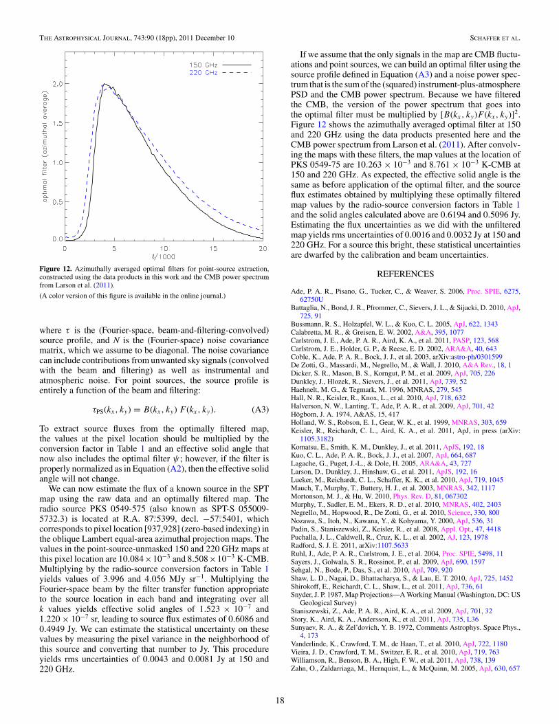
The Astrophysical Journal, 743:90 (18pp), 2011 December 10 Schaffer et al.
Figure 12. Azimuthally averaged optimal filters for point-source extraction,constructed using the data products in this work and the CMB power spectrumfrom Larson et al. (2011).
(A color version of this figure is available in the online journal.)
where τ is the (Fourier-space, beam-and-filtering-convolved)source profile, and N is the (Fourier-space) noise covariancematrix, which we assume to be diagonal. The noise covariancecan include contributions from unwanted sky signals (convolvedwith the beam and filtering) as well as instrumental andatmospheric noise. For point sources, the source profile isentirely a function of the beam and filtering:
τPS(kx, ky) = B(kx, ky) F (kx, ky). (A3)
To extract source fluxes from the optimally filtered map,the values at the pixel location should be multiplied by theconversion factor in Table 1 and an effective solid angle thatnow also includes the optimal filter ψ ; however, if the filter isproperly normalized as in Equation (A2), then the effective solidangle will not change.
We can now estimate the flux of a known source in the SPTmap using the raw data and an optimally filtered map. Theradio source PKS 0549-575 (also known as SPT-S 055009-5732.3) is located at R.A. 87.◦5399, decl. −57.◦5401, whichcorresponds to pixel location [937,928] (zero-based indexing) inthe oblique Lambert equal-area azimuthal projection maps. Thevalues in the point-source-unmasked 150 and 220 GHz maps atthis pixel location are 10.084×10⁻³ and 8.508×10⁻³ K-CMB.Multiplying by the radio-source conversion factors in Table 1yields values of 3.996 and 4.056 MJy sr−1. Multiplying theFourier-space beam by the filter transfer function appropriateto the source location in each band and integrating over allk values yields effective solid angles of 1.523 × 10⁻⁷ and1.220 × 10−7 sr, leading to source flux estimates of 0.6086 and0.4949 Jy. We can estimate the statistical uncertainty on thesevalues by measuring the pixel variance in the neighborhood ofthis source and converting that number to Jy. This procedureyields rms uncertainties of 0.0043 and 0.0081 Jy at 150 and220 GHz.
If we assume that the only signals in the map are CMB fluctu-ations and point sources, we can build an optimal filter using thesource profile defined in Equation (A3) and a noise power spec-trum that is the sum of the (squared) instrument-plus-atmospherePSD and the CMB power spectrum. Because we have filteredthe CMB, the version of the power spectrum that goes intothe optimal filter must be multiplied by [B(kx, ky)F (kx, ky)]2.Figure 12 shows the azimuthally averaged optimal filter at 150and 220 GHz using the data products presented here and theCMB power spectrum from Larson et al. (2011). After convolv-ing the maps with these filters, the map values at the location ofPKS 0549-75 are 10.263 × 10⁻³ and 8.761 × 10⁻³ K-CMB at150 and 220 GHz. As expected, the effective solid angle is thesame as before application of the optimal filter, and the sourceflux estimates obtained by multiplying these optimally filteredmap values by the radio-source conversion factors in Table 1and the solid angles calculated above are 0.6194 and 0.5096 Jy.Estimating the flux uncertainties as we did with the unfilteredmap yields rms uncertainties of 0.0016 and 0.0032 Jy at 150 and220 GHz. For a source this bright, these statistical uncertaintiesare dwarfed by the calibration and beam uncertainties.
REFERENCES
Ade, P. A. R., Pisano, G., Tucker, C., & Weaver, S. 2006, Proc. SPIE, 6275,62750U
Battaglia, N., Bond, J. R., Pfrommer, C., Sievers, J. L., & Sijacki, D. 2010, ApJ,725, 91
Bussmann, R. S., Holzapfel, W. L., & Kuo, C. L. 2005, ApJ, 622, 1343Calabretta, M. R., & Greisen, E. W. 2002, A&A, 395, 1077Carlstrom, J. E., Ade, P. A. R., Aird, K. A., et al. 2011, PASP, 123, 568Carlstrom, J. E., Holder, G. P., & Reese, E. D. 2002, ARA&A, 40, 643Coble, K., Ade, P. A. R., Bock, J. J., et al. 2003, arXiv:astro-ph/0301599De Zotti, G., Massardi, M., Negrello, M., & Wall, J. 2010, A&A Rev., 18, 1Dicker, S. R., Mason, B. S., Korngut, P. M., et al. 2009, ApJ, 705, 226Dunkley, J., Hlozek, R., Sievers, J., et al. 2011, ApJ, 739, 52Haehnelt, M. G., & Tegmark, M. 1996, MNRAS, 279, 545Hall, N. R., Keisler, R., Knox, L., et al. 2010, ApJ, 718, 632Halverson, N. W., Lanting, T., Ade, P. A. R., et al. 2009, ApJ, 701, 42Hogbom, J. A. 1974, A&AS, 15, 417Holland, W. S., Robson, E. I., Gear, W. K., et al. 1999, MNRAS, 303, 659Keisler, R., Reichardt, C. L., Aird, K. A., et al. 2011, ApJ, in press (arXiv:
1105.3182)Komatsu, E., Smith, K. M., Dunkley, J., et al. 2011, ApJS, 192, 18Kuo, C. L., Ade, P. A. R., Bock, J. J., et al. 2007, ApJ, 664, 687Lagache, G., Puget, J.-L., & Dole, H. 2005, ARA&A, 43, 727Larson, D., Dunkley, J., Hinshaw, G., et al. 2011, ApJS, 192, 16Lueker, M., Reichardt, C. L., Schaffer, K. K., et al. 2010, ApJ, 719, 1045Mauch, T., Murphy, T., Buttery, H. J., et al. 2003, MNRAS, 342, 1117Mortonson, M. J., & Hu, W. 2010, Phys. Rev. D, 81, 067302Murphy, T., Sadler, E. M., Ekers, R. D., et al. 2010, MNRAS, 402, 2403Negrello, M., Hopwood, R., De Zotti, G., et al. 2010, Science, 330, 800Nozawa, S., Itoh, N., Kawana, Y., & Kohyama, Y. 2000, ApJ, 536, 31Padin, S., Staniszewski, Z., Keisler, R., et al. 2008, Appl. Opt., 47, 4418Puchalla, J. L., Caldwell, R., Cruz, K. L., et al. 2002, AJ, 123, 1978Radford, S. J. E. 2011, arXiv:1107.5633Ruhl, J., Ade, P. A. R., Carlstrom, J. E., et al. 2004, Proc. SPIE, 5498, 11Sayers, J., Golwala, S. R., Rossinot, P., et al. 2009, ApJ, 690, 1597Sehgal, N., Bode, P., Das, S., et al. 2010, ApJ, 709, 920Shaw, L. D., Nagai, D., Bhattacharya, S., & Lau, E. T. 2010, ApJ, 725, 1452Shirokoff, E., Reichardt, C. L., Shaw, L., et al. 2011, ApJ, 736, 61Snyder, J. P. 1987, Map Projections—A Working Manual (Washington, DC: US
Geological Survey)Staniszewski, Z., Ade, P. A. R., Aird, K. A., et al. 2009, ApJ, 701, 32Story, K., Aird, K. A., Andersson, K., et al. 2011, ApJ, 735, L36Sunyaev, R. A., & Zel’dovich, Y. B. 1972, Comments Astrophys. Space Phys.,
4, 173Vanderlinde, K., Crawford, T. M., de Haan, T., et al. 2010, ApJ, 722, 1180Vieira, J. D., Crawford, T. M., Switzer, E. R., et al. 2010, ApJ, 719, 763Williamson, R., Benson, B. A., High, F. W., et al. 2011, ApJ, 738, 139Zahn, O., Zaldarriaga, M., Hernquist, L., & McQuinn, M. 2005, ApJ, 630, 657
18