Comparison between the finite differences, finite volume ...

Vincent Chiaruttini, Georges CailletaudVincent Chiaruttini, Georges [email protected]@onera.fr
Non Linear Computational Mechanics Athens MP06/2012–Non Linear Computational Mechanics Athens MP06/2012–
The Finite Element method forThe Finite Element method fornonlinear structural problemsnonlinear structural problems

2 FE analysis for non linear mechanics Athens MP06 - V.Chiaruttini–FE analysis for non linear mechanics Athens MP06 - V.Chiaruttini–
OutlineOutline
Generalities on computational strategies for nonlinear problemsExamples (contact, crack propagation, non-linear behaviour, geometrical non-linearities)
Classical algorithm for nonlinear or time dependant problems
Local numerical aspects of plasticityElastic-plastic behaviour
Local integration of non-linear models
Global numerical aspects of plasticitySolution process
Consistent tangent matrix
Examples of solution process
Presentation of Z-mat

3 FE analysis for non linear mechanics Athens MP06 - V.Chiaruttini–FE analysis for non linear mechanics Athens MP06 - V.Chiaruttini–
Non-linearities in structural problemsNon-linearities in structural problems
Contact
Due to the non-penetration condition
Crack propagation problem under time dependant loading
When crack propagates the solution becomes non-linearly time dependant
Geometrical nonlinearities
For large deformation, instabilities can also occur (buckling)
Nonlinear constitutive relationship
Non linear behaviour: elastoplasticity, damage, viscosity

4 FE analysis for non linear mechanics Athens MP06 - V.Chiaruttini–FE analysis for non linear mechanics Athens MP06 - V.Chiaruttini–
Solution processSolution process
Iterative algorithmScalar example
For any kind of regular function, no direct process exists
Iterative algorithmStop when a convergence criterion is satisfied
Newton methodBuilt on the linear verification of the first order Taylor development nullity
¯nding u j f(u) = 0
building un ! u j f(u) = 0rank k j jf(uk)j < "crit
f(uk+1) ¼ f(uk) + (uk+1 ¡ uk) f0(uk) = 0
u0 u2u1
f(u)
u
) uk+1 = uk ¡ f(uk)=f0(uk)

5 FE analysis for non linear mechanics Athens MP06 - V.Chiaruttini–FE analysis for non linear mechanics Athens MP06 - V.Chiaruttini–
Solution processSolution process
Newton methodBuilt on the linear verification of the first order Taylor development nullity
Convergence depends on u0
When convergesRank k errorRecurrence on error relationshipTaylor expansion closely to the exact solution
Quadratic convergenceClose enough to the solution each iteration produces twice more significant new digits
f(uk+1) ¼ f(uk) + (uk+1 ¡ uk) f0(uk) = 0
) uk+1 = uk ¡ f(uk)=f0(uk)
ek = uk ¡ uek+1 ¡ ek = uk+1 ¡ uk = ¡f(uk)=f 0(uk)
f (uk) = f 0(u)ek +1
2f 00(u)e2k + o(e2k)
f 0(uk) = f 0(u) + f 00(u)ek + f 000(u)e2k + o(e2k)
ek+1 = ek ¡2f 0ek + f 00e2k
2f 0 + f 00ek + f 000e2k+ o(e2k) =
f 00(u)2f 0(u)
e2k + o(e2k) = O(e2k)

6 FE analysis for non linear mechanics Athens MP06 - V.Chiaruttini–FE analysis for non linear mechanics Athens MP06 - V.Chiaruttini–
Solution processSolution process
Newton methodQuadratic convergence
Require to update the derivative at each iteration
Modified Newton methodsConstant direction
Linear convergence ek+1 = (1¡ f 0(u)=K)ek + o(jekj) = O(jekj)
f 0(uk) ¼ K = cst = f 0(u0)
u0 u2u1
f(u)
u
uk+1 = uk ¡ f(uk)=K

7 FE analysis for non linear mechanics Athens MP06 - V.Chiaruttini–FE analysis for non linear mechanics Athens MP06 - V.Chiaruttini–
Solution processSolution process
Newton methodQuadratic convergence
Require to update the derivative at each iteration
Modified Newton methodsConstant direction Linear convergenceSecant update
Golden ratio convergence order
u0 u2u1
f(u)
u
f 0(uk) ¼ K = cst = f 0(u0)
uk+1 = uk + f(uk)uk ¡ uk¡1
f(uk)¡ f(uk¡1)ek+1 = O(jekj
1+p5
2 )
8 FE analysis for non linear mechanics Athens MP06 - V.Chiaruttini–FE analysis for non linear mechanics Athens MP06 - V.Chiaruttini–
Solution processSolution process
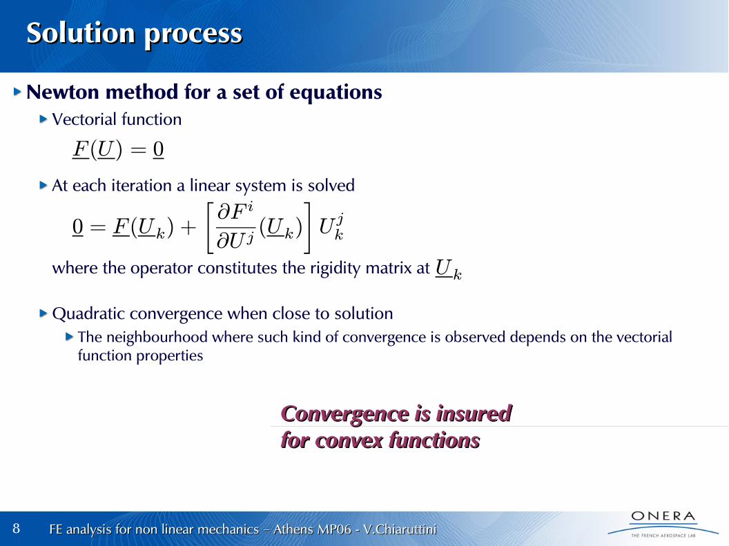
Newton method for a set of equationsVectorial function
At each iteration a linear system is solved
where the operator constitutes the rigidity matrix at
Quadratic convergence when close to solutionThe neighbourhood where such kind of convergence is observed depends on the vectorial function properties
F (U) = 0
0 = F (Uk) +
·@F i
@U j(Uk)
¸U jk
Uk
Convergence is insuredConvergence is insuredfor convex functionsfor convex functions

9 FE analysis for non linear mechanics Athens MP06 - V.Chiaruttini–FE analysis for non linear mechanics Athens MP06 - V.Chiaruttini–
Examples of convergence using a Newton algorithmExamples of convergence using a Newton algorithm

10 FE analysis for non linear mechanics Athens MP06 - V.Chiaruttini–FE analysis for non linear mechanics Athens MP06 - V.Chiaruttini–
Examples of convergence using a Newton algorithmExamples of convergence using a Newton algorithm

11 FE analysis for non linear mechanics Athens MP06 - V.Chiaruttini–FE analysis for non linear mechanics Athens MP06 - V.Chiaruttini–
ODE integrationODE integration
Time dependant problem are ruled by differential equationsReduce high order differential systems to first order
General formulation
Euler-type integration schemesFinite difference time discretization
θ-method (method-B)
Explicit Forward Euler (θ=0) Crank-Nicholson (θ=0.5) Implicit Euler (θ=1)Conditionally stable Unconditionally stable Unconditionally stable1st order accurate 2nd order accurate 1st order accurate
d2y
dt2+ g(t)
dy
dt= r(t) ,
½dydt = z(t)dzdt = r(t) ¡ g(t) z(t)
[ _Y ] = [F (t; [Y ])] [ _Y (t = t0)] = [Y0]
_Y (t) = F (t; Y )
Y n+1 ¡ Y n¢t
= µFn+1(Y n+1) + (1¡ µ)Fn(Y n)
forward methods _Y (tn+1) ¼Y n+1 ¡ Y n
¢t
Y (tn) = Yn; tn+1 = tn +¢t

12 FE analysis for non linear mechanics Athens MP06 - V.Chiaruttini–FE analysis for non linear mechanics Athens MP06 - V.Chiaruttini–
ODE integrationODE integration
Time dependant problem are ruled by differential equationsRunge-Kutta explicit integration
Minimal multiple evaluations of on a given time increment to insure a specific order accuracy, based on Taylor expansionRK1 is the forward explicit Euler schemeRK2 using one mid-point sub calculation at
2nd order method
RK4 popular method using 4 sub calculations
4th order method
F (t; y(t))
tn+ 12
yn+1 = yn +¢t f¡tn+1=2; yn+1=2
¢yn+1=2 = yn +
¢t
2f (tn; yn)
yn+1 = yn +¢t=6 (k1 + 2k2 + 2k3 + k4)
k1 = f(tn; yn)
k4 = f(tn+1=2; yn +¢tk3)
k2 = f(tn+1=2; yn + (¢t=2)k1)k3 = f(tn+1=2; yn + (¢t=2)k2)
Initial slope on the interval
Mid interval slope using k1
Mid interval slope using k2
Final slope using k3 on the interval
yn+1 = yn +¢ty0n + (¢t=2)y00n + o(¢t2)

13 FE analysis for non linear mechanics Athens MP06 - V.Chiaruttini–FE analysis for non linear mechanics Athens MP06 - V.Chiaruttini–
OutlineOutline
Generalities on computational strategies for nonlinear problemsExamples (contact, crack propagation, non-linear behaviour, geometrical non-linearities)
Classical algorithm for nonlinear or time dependant problems
Local numerical aspects of plasticityElastic-plastic behaviour
Local integration of non-linear models
Global numerical aspects of plasticitySolution process
Consistent tangent matrix
Examples of solution process
Presentation of Z-mat
14 FE analysis for non linear mechanics Athens MP06 - V.Chiaruttini–FE analysis for non linear mechanics Athens MP06 - V.Chiaruttini–
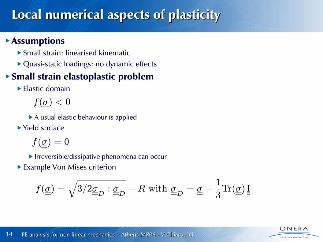
Local numerical aspects of plasticityLocal numerical aspects of plasticity
AssumptionsSmall strain: linearised kinematicQuasi-static loadings: no dynamic effects
Small strain elastoplastic problemElastic domain
A usual elastic behaviour is applied
Yield surface
Irreversible/dissipative phenomena can occur
Example Von Mises criterion
f(¾) < 0
f(¾) = 0
f(¾) =q3=2¾
D: ¾
D¡R with ¾
D= ¾ ¡ 1
3Tr(¾) I

15 FE analysis for non linear mechanics Athens MP06 - V.Chiaruttini–FE analysis for non linear mechanics Athens MP06 - V.Chiaruttini–
Local numerical aspects of plasticityLocal numerical aspects of plasticity
Small strain elastoplastic problemPlastic strain
Strain partition
Rigidity
Yield surface evolution (convex), hardeningWhen the yield surface evolves
Isotropic hardening yield surface increase→Kinematic hardening yield surface translation→
Flow rulesPlasticity (normality rule)
Cumulated plastic strain rate
" = "e + "in = "e + "p
¾ = A : "e = A : (" ¡ "p)
_"p = _ @f
@¾; _ ¸ 0; f(¾) · 0; _ f(¾) = 0
p(t) =
Z t
0
r3
2
¡_"p(¿) : _"p(¿)
¢d¿³= _ for a Von Mises criterion
´
f = 0

16 FE analysis for non linear mechanics Athens MP06 - V.Chiaruttini–FE analysis for non linear mechanics Athens MP06 - V.Chiaruttini–
Local numerical aspects of plasticityLocal numerical aspects of plasticity
Common formalism for viscoplasticity/multipotentials/large strainStrain partition
Small strain Large strain
Elasticity
Flow rulesPlasticity (state must stay on the yield surface at the end of the increment)
Viscoplasticity (state expected to be on the relevant equipotential at the end of the increment)
Hardening rules
" = "e + "in = "e + "p + "vp F = E P
¾ = A : "e
_"p =X
s
_ sns
_"vp =X
s
_vsms
_ s from _fs = 0
_vs =
¿f s
K
Àn
_YI = fct(YI ; "p; "vp)

17 FE analysis for non linear mechanics Athens MP06 - V.Chiaruttini–FE analysis for non linear mechanics Athens MP06 - V.Chiaruttini–
Numerical solution processNumerical solution process
Elastoplastic exampleRelations
Equilibrium and strain definition
Behaviour
Boundary conditions (initial equilibrium and no plasticity)
r¾ + f = 0 " =1
2
¡r u+rT u
¢
t 2 [0; T ]
_p ¸ 0 ¾eq ¡R(p) · 0_"p = _p3
2¾eq¾D
u = ud on @u
¾ ¢ n = F on @f
²p(t = 0) = 0
¾ = A : ("¡ "p)
_p (¾eq ¡R(p)) = 0
¾eq =
r3
2k¾
Dk

18 FE analysis for non linear mechanics Athens MP06 - V.Chiaruttini–FE analysis for non linear mechanics Athens MP06 - V.Chiaruttini–
Numerical solution processNumerical solution process
Elastoplastic exampleMechanical stateTemporal discretization
Incremental temporal approach using a regular gridThe solution is search incrementaly at each time step tn+1 (all previous step states being known)
Spatial discretizationFE method in displacement
Nonlinearity comes from the non linear relation between stress and strain relation
Local integration of the mechanical behaviourAt each point of the structure process is defined by the following process
Global equilibriumVerified by the solution of the nonlinear variational formulation
tn+1 = tn +¢t
8u¤ 2 U0ad;Z
¾n+1
: "¤d =
Z
fn+1
:u¤d+
Z
@F
Fn+1:u¤dS
S(x; t) =©u(x; t); "(x; t); "p(x; t); ¾(x; t)
ª
(un+1;Sn) ! ¾n+1
= F(un+1;Sn)
R(un+1;u¤;Sn) = 0;8u¤ 2 U0ad

19 FE analysis for non linear mechanics Athens MP06 - V.Chiaruttini–FE analysis for non linear mechanics Athens MP06 - V.Chiaruttini–
Local behaviour integration processLocal behaviour integration process
Generic interface for any constitutive equationGauss point process (where the element variational formulation is integrated)Definition
External parameters (ep) imposed as inputIntegrated variables (vint)Auxiliary variables (vaux) just for outputCoefficients (coef) material parametersPrimal and dual variables prescribed variables and associated fluxes
Primal: strain increment on the current time interval (input to the local integration process)Dual: stress obtained useful for variational formulation (as output of the local integration process)
Local GP integration ODE integration to get
vint, vaux, dual variables
Dual variablesPrimal variables
"p; "
p
¾
F(un+1;Sn)

20 FE analysis for non linear mechanics Athens MP06 - V.Chiaruttini–FE analysis for non linear mechanics Athens MP06 - V.Chiaruttini–
Local behaviour integration processLocal behaviour integration process
Time integrationNormality rule as an ODE
Explicit integration Runge-Kutta (RK4 usually, beware of stability condition)→
Implicit integration → θ-methods (stable but requires a local Jacobian computation)
_"p = _p3
2¾eq¾D
, "pn+1
= "pn+
Z tn+1
tn
_"p(¿) d¿

21 FE analysis for non linear mechanics Athens MP06 - V.Chiaruttini–FE analysis for non linear mechanics Athens MP06 - V.Chiaruttini–
Local behaviour integration processLocal behaviour integration process
Elastic prediction and correction algorithmSolution depends on the test (is the evolution purely elastic on ∆t ?)
Elastic prediction
Convexity of the yield surface gives
purely elastic evolution, prediction is correct
Else a plastic evolution is observedA correction must be applied on the elastic prediction
where is the outward unit normal to the final yeld surface
¾eq ¡R(p) · 0
¾en+1
= ¾n+A : ¢"e
n
f(¾en+1
; pn) ¸ f(¾n+1
; pn +¢pn)
f(¾en+1
; pn) · 0
8<:
¾n+1
= ¾en+1
"pn+1
= "pn
pn+1 = pn
¢pn > 0; ¢pn f(¾n+1; pn +¢pn) = 0 ) f(¾n+1
; pn +¢pn) = 0
¾n+1
= ¾en+1
¡A : ¢"pn
¢"pn= ¢pn
r3
2Nn+1
¢pn > 0
Nn+1

22 FE analysis for non linear mechanics Athens MP06 - V.Chiaruttini–FE analysis for non linear mechanics Athens MP06 - V.Chiaruttini–
Local behaviour integration processLocal behaviour integration process
Elastic prediction and correction algorithmSolution depends on the test (is the evolution purely elastic on ∆t ?)
Elastic prediction
Convexity of the yield surface gives
purely elastic evolution, prediction is correct
Else a plastic evolution is observedA correction must be applied on the elastic prediction
where is the outward unit normal to the final yeld surface
¾eq ¡R(p) · 0
¾en+1
= ¾n+A : ¢"e
n
f(¾en+1
; pn) ¸ f(¾n+1
; pn +¢pn)
f(¾en+1
; pn) · 0
8<:
¾n+1
= ¾en+1
"pn+1
= "pn
pn+1 = pn
¢pn > 0; ¢pn f(¾n+1; pn +¢pn) = 0 ) f(¾n+1
; pn +¢pn) = 0
¾n+1
= ¾en+1
¡A : ¢"pn
¢"pn= ¢pn
r3
2Nn+1
¢pn > 0
Nn+1

23 FE analysis for non linear mechanics Athens MP06 - V.Chiaruttini–FE analysis for non linear mechanics Athens MP06 - V.Chiaruttini–
Radial return algorithmRadial return algorithm
For von Mises based criteria or isotropic or linear kinematic hardeningThe corrective term is oriented by the final normal that can be computed a priori
For von Mises criterion the final normal is collinear to the elastic predictor deviator
Lamé coefficient
Final state on the yeld surface gives to verify
that allows to find
A : ¢"pn
Nn+1
=¾eDn+1
k¾eDn+1
k ¾n+1
= ¾en+1
¡A : ¢pn
r3
2Nn+1
¹¾eqn+1 = ¾e;eqn+1 ¡ 3¹¢pn
¾e;eqn+1 ¡ 3¹¢pn ¡R(pn +¢pn) = 0
¢pn
f(¾n+1; pn+1) = 0
f(¾n; pn) = 0
¾Dn
¾Dn+1
¾eDn+1

24 FE analysis for non linear mechanics Athens MP06 - V.Chiaruttini–FE analysis for non linear mechanics Athens MP06 - V.Chiaruttini–
Generalized radial return algorithmGeneralized radial return algorithm
Closest point projection techniqueFor a generalized normality rule
Fluxes
f(¾n+1; pn+1) = 0
f(¾n; pn) = 0
¾Dn
¾Dn+1
¾eDn+1
¢"p =@f
@¾¢p ¢®I =
@f
@YI¢p
¢¾ = A :¡¢"¡¢"P
¢
¢YI =MI ¢®I
¢§ =
·¢¾¢YI
¸=
"A : ¢"
0
#¡"
A 0
0 MI
#"@f@¾@f@YI
#¢p

25 FE analysis for non linear mechanics Athens MP06 - V.Chiaruttini–FE analysis for non linear mechanics Athens MP06 - V.Chiaruttini–
Generic formulation of the local integration processGeneric formulation of the local integration process
26 FE analysis for non linear mechanics Athens MP06 - V.Chiaruttini–FE analysis for non linear mechanics Athens MP06 - V.Chiaruttini–
OutlineOutline
Generalities on computational strategies for nonlinear problemsExamples (contact, crack propagation, non-linear behaviour, geometrical non-linearities)
Classical algorithm for nonlinear or time dependant problems
Local numerical aspects of plasticityElastic-plastic behaviour
Local integration of non-linear models
Global numerical aspects of plasticitySolution process
Consistent tangent matrix
Examples of solution process
Presentation of Z-mat
27 FE analysis for non linear mechanics Athens MP06 - V.Chiaruttini–FE analysis for non linear mechanics Athens MP06 - V.Chiaruttini–
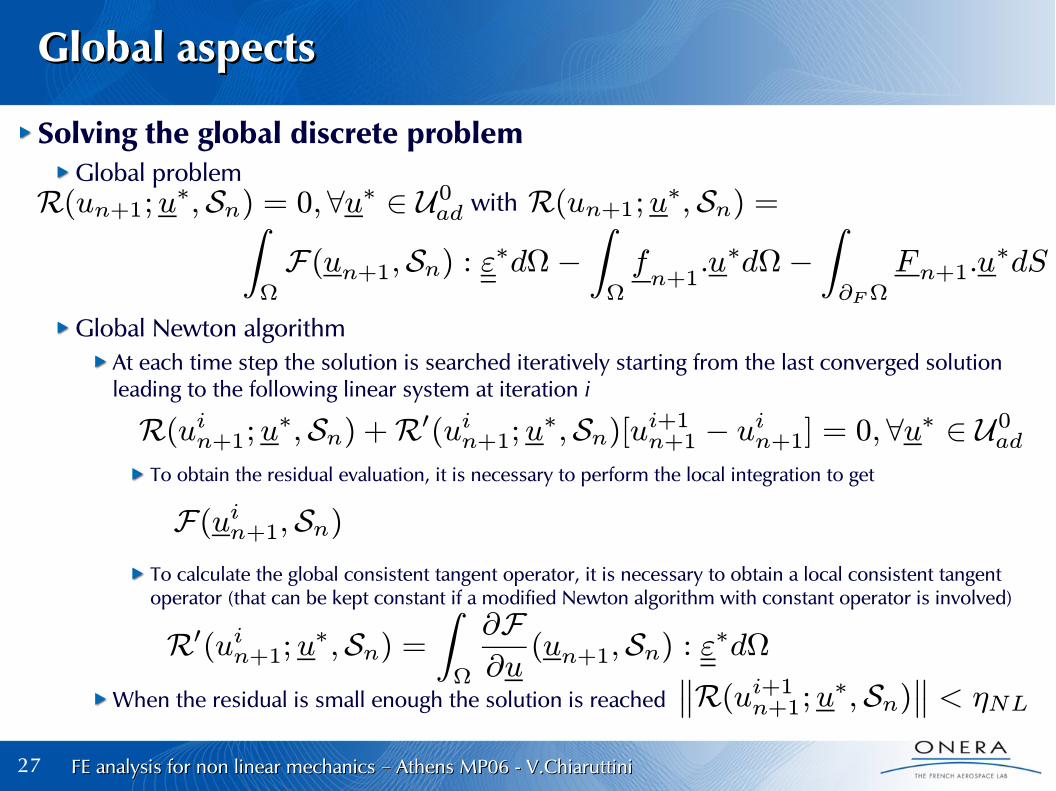
Global aspectsGlobal aspects
Solving the global discrete problemGlobal problem
with
Global Newton algorithmAt each time step the solution is searched iteratively starting from the last converged solution leading to the following linear system at iteration i
To obtain the residual evaluation, it is necessary to perform the local integration to get
To calculate the global consistent tangent operator, it is necessary to obtain a local consistent tangent operator (that can be kept constant if a modified Newton algorithm with constant operator is involved)
When the residual is small enough the solution is reached
R(un+1;u¤;Sn) = 0;8u¤ 2 U0adZ
F(un+1;Sn) : "¤d¡Z
fn+1
:u¤d¡Z
@F
Fn+1:u¤dS
R(un+1;u¤;Sn) =
F(uin+1;Sn)
R(uin+1;u¤;Sn) +R0(uin+1;u¤;Sn)[ui+1n+1 ¡ uin+1] = 0; 8u¤ 2 U0ad
R0(uin+1; u¤;Sn) =Z
@F@u
(un+1;Sn) : "¤d°°R(ui+1n+1;u¤;Sn)
°° < ´NL

28 FE analysis for non linear mechanics Athens MP06 - V.Chiaruttini–FE analysis for non linear mechanics Athens MP06 - V.Chiaruttini–
Local consistent tangent operatorLocal consistent tangent operator
In the local integration process

29 FE analysis for non linear mechanics Athens MP06 - V.Chiaruttini–FE analysis for non linear mechanics Athens MP06 - V.Chiaruttini–
OutlineOutline
Generalities on computational strategies for nonlinear problemsExamples (contact, crack propagation, non-linear behaviour, geometrical non-linearities)
Classical algorithm for nonlinear or time dependant problems
Local numerical aspects of plasticityElastic-plastic behaviour
Local integration of non-linear models
Global numerical aspects of plasticitySolution process
Consistent tangent matrix
Examples of solution process
Presentation of Z-mat

30 FE analysis for non linear mechanics Athens MP06 - V.Chiaruttini–FE analysis for non linear mechanics Athens MP06 - V.Chiaruttini–
Viscoelastic with isotropic hardeningViscoelastic with isotropic hardening

31 FE analysis for non linear mechanics Athens MP06 - V.Chiaruttini–FE analysis for non linear mechanics Athens MP06 - V.Chiaruttini–
Viscoelastic with isotropic hardeningViscoelastic with isotropic hardeningImplementationImplementation
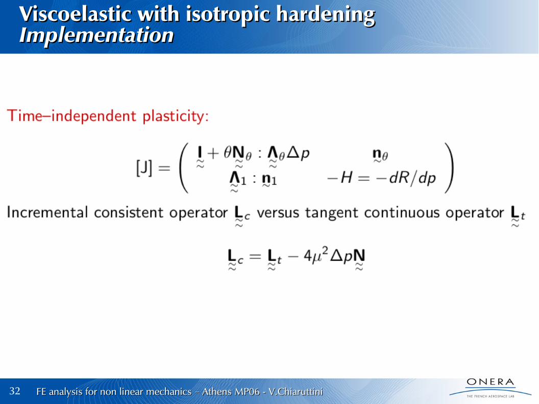
32 FE analysis for non linear mechanics Athens MP06 - V.Chiaruttini–FE analysis for non linear mechanics Athens MP06 - V.Chiaruttini–
Viscoelastic with isotropic hardeningViscoelastic with isotropic hardeningImplementationImplementation

33 FE analysis for non linear mechanics Athens MP06 - V.Chiaruttini–FE analysis for non linear mechanics Athens MP06 - V.Chiaruttini–
Viscoelastic with isotropic hardeningViscoelastic with isotropic hardeningImplementationImplementation

34 FE analysis for non linear mechanics Athens MP06 - V.Chiaruttini–FE analysis for non linear mechanics Athens MP06 - V.Chiaruttini–
Large strain viscoelastic with isotropic hardening Large strain viscoelastic with isotropic hardening

35 FE analysis for non linear mechanics Athens MP06 - V.Chiaruttini–FE analysis for non linear mechanics Athens MP06 - V.Chiaruttini–
System of residualsSystem of residuals

36 FE analysis for non linear mechanics Athens MP06 - V.Chiaruttini–FE analysis for non linear mechanics Athens MP06 - V.Chiaruttini–
AlgorithmAlgorithm

37 FE analysis for non linear mechanics Athens MP06 - V.Chiaruttini–FE analysis for non linear mechanics Athens MP06 - V.Chiaruttini–
Tangent matrixTangent matrix

38 FE analysis for non linear mechanics Athens MP06 - V.Chiaruttini–FE analysis for non linear mechanics Athens MP06 - V.Chiaruttini–
OutlineOutline
Generalities on computational strategies for nonlinear problemsExamples (contact, crack propagation, non-linear behaviour, geometrical non-linearities)
Classical algorithm for nonlinear or time dependant problems
Local numerical aspects of plasticityElastic-plastic behaviour
Local integration of non-linear models
Global numerical aspects of plasticitySolution process
Consistent tangent matrix
Examples of solution process
Presentation of Z-mat

39 FE analysis for non linear mechanics Athens MP06 - V.Chiaruttini–FE analysis for non linear mechanics Athens MP06 - V.Chiaruttini–
Presentation of the Z-mat libraryPresentation of the Z-mat library

40 FE analysis for non linear mechanics Athens MP06 - V.Chiaruttini–FE analysis for non linear mechanics Athens MP06 - V.Chiaruttini–
Inside Z-matInside Z-mat
41 FE analysis for non linear mechanics Athens MP06 - V.Chiaruttini–FE analysis for non linear mechanics Athens MP06 - V.Chiaruttini–
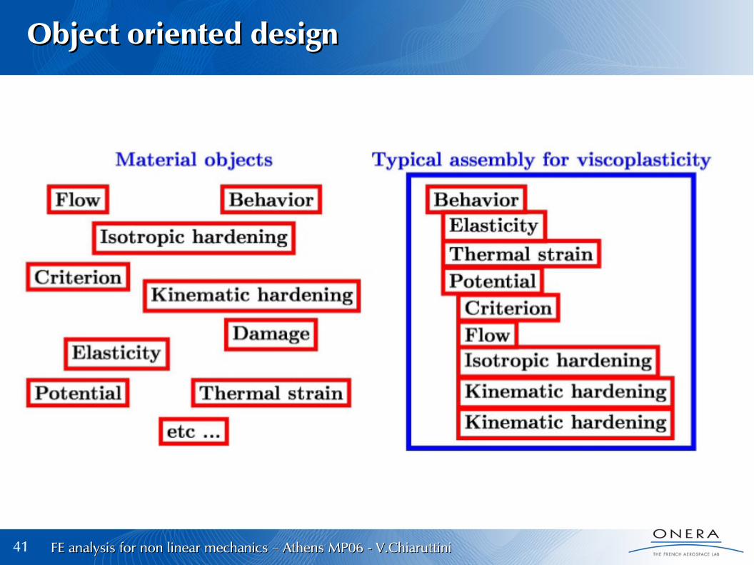
Object oriented designObject oriented design

42 FE analysis for non linear mechanics Athens MP06 - V.Chiaruttini–FE analysis for non linear mechanics Athens MP06 - V.Chiaruttini–
Isotropic and non-linear kinematic modelIsotropic and non-linear kinematic model

43 FE analysis for non linear mechanics Athens MP06 - V.Chiaruttini–FE analysis for non linear mechanics Athens MP06 - V.Chiaruttini–
Datafile examplesDatafile examples

44 FE analysis for non linear mechanics Athens MP06 - V.Chiaruttini–FE analysis for non linear mechanics Athens MP06 - V.Chiaruttini–
ZebFront interface layer for efficientZebFront interface layer for efficientbehaviour developmentbehaviour development
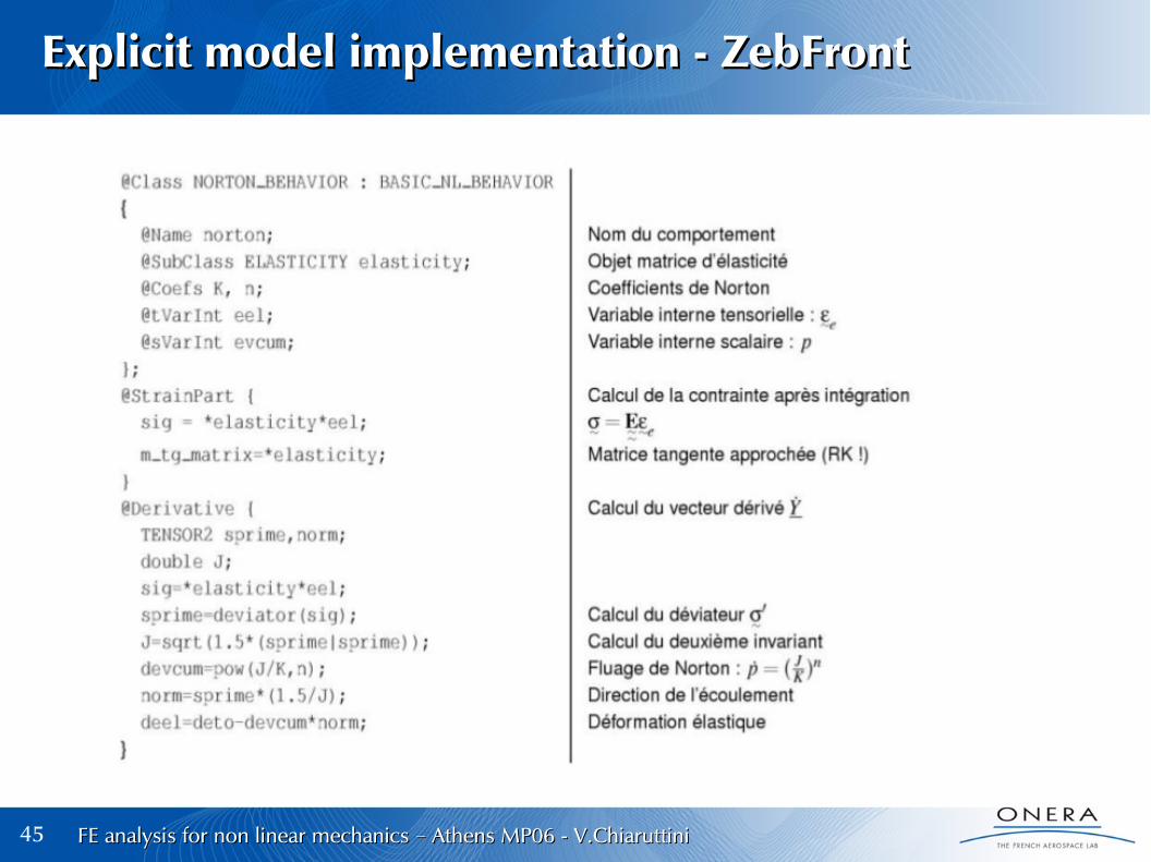
45 FE analysis for non linear mechanics Athens MP06 - V.Chiaruttini–FE analysis for non linear mechanics Athens MP06 - V.Chiaruttini–
Explicit model implementation - ZebFrontExplicit model implementation - ZebFront

46 FE analysis for non linear mechanics Athens MP06 - V.Chiaruttini–FE analysis for non linear mechanics Athens MP06 - V.Chiaruttini–
Implicit model implementation - ZebFrontImplicit model implementation - ZebFront

47 FE analysis for non linear mechanics Athens MP06 - V.Chiaruttini–FE analysis for non linear mechanics Athens MP06 - V.Chiaruttini–
Multimat capabilitiesMultimat capabilities

48 FE analysis for non linear mechanics Athens MP06 - V.Chiaruttini–FE analysis for non linear mechanics Athens MP06 - V.Chiaruttini–
Multimat capabilitiesMultimat capabilities

FE analysis for non linear mechanics Athens MP06 - V.Chiaruttini–FE analysis for non linear mechanics Athens MP06 - V.Chiaruttini–
ReferencesReferences
Bonnet M., Frangi A. (2006)Analyse des solides déformables par la méthode des éléments finis. Editions Ecole Polytechnique.Belytschko, T., Liu, W., and Moran, B. (2000).Nonlinear Finite Elements for Continua and Structures.Besson, J., Cailletaud, G., Chaboche, J.-L., and Forest, S. (2001).Mecanique non linéaire des matériaux. Hermes.–Ciarlet, P. and Lions, J. (1995).Handbook of Numerical Analysis : Finite Element Methods (P.1), Numerical Methods for Solids (P.2). North Holland.Dhatt, G. and Touzot, G. (1981).Une présentation de la méthode des élements finis. Maloine.Hughes, T. (1987).The finite element method: Linear static and dynamic finite element analysis. Prentice Hall –Inc.Simo, J. and Hughes, T. (1997).Computational Inelasticity. Springer Verlag.Zienkiewicz, O. and Taylor, R. (2000).The finite element method, Vol. I-III (Vol.1: The Basis, Vol.2: Solid Mechanics, Vol. 3: Fluid dynamics). Butterworth Heinemann.–