The Financial Projection Model 2.0 and its Implementation...

The Financial Projection Model 2.0

and its Implementation into

Stress Testing and Other Projections

Murat Arslaner

The author is a Financial Sector Specialist in the Finance and Markets Global Practice of the World Bank ([email protected]). The author would like to acknowledge the significant contributions of Ines Gonzalez Del Mazo for editorial support. The author would also like to thank Mario Guadamillas, Aquiles A. Almansi, Joaquin G. Gutierrez, James Seward, Martin Melecky, Vahe Vardanyan, Attila Csajbok, Jorge G Patino for their time in review of drafts and their many useful comments. The views presented in the paper do not necessarily represent the views of the World Bank.

1

Contents

Abbreviations and Acronyms ....................................................................................................................... 3 Executive Summary ...................................................................................................................................... 4 Background ................................................................................................................................................... 5 Uses of the Model ......................................................................................................................................... 5

Viability Assessment ................................................................................................................................ 6 Liquidation Value (Cost) .......................................................................................................................... 7 Present Value ............................................................................................................................................ 7 Other Projections ...................................................................................................................................... 7

Potential Users of the Model ......................................................................................................................... 8 Prerequisites for the Robust Uses of the Model ............................................................................................ 8

Diagnostic ................................................................................................................................................. 8 Data ........................................................................................................................................................... 8 Skills ......................................................................................................................................................... 9

Disclaimer for Using the Model.................................................................................................................... 9 The Model`s Main Features ........................................................................................................................ 10 The Structure of the Model ......................................................................................................................... 13 The Core Methodology ............................................................................................................................... 14

General .................................................................................................................................................... 14 Sequence of Projections and Balancing Mechanism .............................................................................. 15

Data Requirement and Historical (Trend) Information ............................................................................... 19 Implied Assumptions .................................................................................................................................. 22 Projections Assumptions ............................................................................................................................. 23 Baseline Projection ..................................................................................................................................... 23 Projection Horizon ...................................................................................................................................... 24 Projections: Static or Dynamic Balance Sheet ............................................................................................ 24 Analyzing Projection Results ...................................................................................................................... 25 Viability Assessment .................................................................................................................................. 26

General .................................................................................................................................................... 26 Risk Parameters ...................................................................................................................................... 28 Inputting Risk Parameters into the Model .............................................................................................. 29 Metrics .................................................................................................................................................... 29 Individual or System-Wide Projections .................................................................................................. 31

Liquidation Value Calculation .................................................................................................................... 34 Present Value Calculation ........................................................................................................................... 35 Appendix B. Methodology in Mathematical Notation ................................................................................ 45 Appendix C. Viability and Performance Indicators .................................................................................... 48 Appendix D. The World Bank Terms and Conditions ................................................................................ 49

2

Figures and Tables

Figure 1. Common uses of the Model Figure 2. Structure of FPM 2.0 Figure 3. Dashboard Tab of FPM 2.0 Figure 4. Architecture of FPM 2.0 Figure 5. A projection of the Balance Sheet, Profit Loss Accounts, Funds Flows, Capital Adequacy Ratios, and Liquidity Ratios from the base period to period one Figure 6. Projections for financial and regulatory reports based on positive or negative net Funds Flow Figure 7. Kinds of information that can be derived from historical data Figure 8. Structure of the data entry process Figure 9. Complementing FPM 2.0 with macro scenarios Figure 10. Transmission of shocks in the banking system Table 1. The IMF’s next generation stress testing tools versus the World Bank Group’s FPM 2.0 Table 2. Types of reports that can be inputted in the Model Table 3. Main risks and risk factors used in a viability assessment

3

Abbreviations and Acronyms AFS Available for sale BS Balance sheet CAMEL Capital Adequacy, Asset Quality, Management Capability, Earnings, and

Liquidity CAR Capital adequacy ratio CB Central bank ELA Emergency lending assistance FF Funds flow FX Foreign exchange FPM Financial Projection Model HFT Held for trading HTM Held-to-maturity IMF International Monetary Fund LGD Losses given default LR Liquidity ratio NFL Nonperforming loan NIM Net Interest Margin PD Probability of default PLA Profit loss accounts ROA Return on Assets ROE Return on Equity RR Reserve Requirement RWA Risk-weighted assets

4

Executive Summary This technical note explains the methodology and possible uses of the updated version of the Financial Projection Model (FPM 2.0). This new version of the Model reflects the comments and suggestions from internal World Bank Group staff and supervisory authorities. The updated version has a more user friendly interface, improved methodologies, simplified structure, and easier process for inputting data and developing projection assumptions. The Model is a projection tool that can be used to project banks’ financial statements (balance sheet and income statement), as well as regulatory rates and performance indicators (capital adequacy, liquidity, and foreign exchange position ratios), based on a set of assumptions regarding the banks` assets, liabilities, capital, liquidity, foreign exchange position, incomes, and expenses. The Model assists in assessing the viability, liquidation value, and present value of a bank under consideration. As a projection tool, the Model can also be used in other projections, such as recapitalization, business planning, merger, reorganization, and restructuring, as long as the required data are available and relevant assumptions are developed in a coherent and consistent way. The Model was developed to assist supervisors and regulators in their duties. As a multipurpose analytical tool, the FPM 2.0 can help the authorities improve their analytical capacity on assessing the vulnerability of the banking system on an individual and system-wide basis. Other potential users include banks, which could use the Model to project their performance and results. The Model’s key factors for effective and precise performance are quality data and user’s expertise. The Model is a predesigned tool that projects data over time; therefore, the quality and the granularity of data will have consequences for the model’s results. In addition, users need to have the technical skills and knowledge related to financial reporting and analysis of banks, financial projections, and scenario development to create assumptions that will lead to robust results. Other information about the bank’s business model will also contribute to accuracy. In conclusion, the Model, if used correctly, can be a powerful analytical tool that can provide a technically solid and clear perspective of the financial dynamics of banks in a reasonably rapid and efficient manner. In addition, it can be complemented by other analytical tools, such as econometric models, that would help in the development of more consistent and realistic scenarios.

5

Background The first version of the Financial Projection Model (FPM) was developed by Murat Arslaner, Joon Soo Lee, and Joaquin Gutierrez to assess the financial condition of a bank over a projected horizon under a set of assumptions. The Model was unique in terms of allowing users to perform an integrated risk assessment taking into account the linkages among credit, interest rate, and liquidity risks and second-round effects in a forward-looking way. The team, under Joaquin Gutierrez`s lead, started to develop the Model in 2008, when the global financial crisis emerged, with the objective of helping authorities in assessing the risks faced by individual banks and developing corrective actions to address the buildup of those risks. The Model was inspired in different degrees by previous models developed since 1982 by Joaquin Gutierrez, Alfredo Bello, and Sophie Sirtaine in their respective work and engagements, but the new version does not replicate the models generated by these authors. The new version, FPM 2.0, features improved methodologies and a simplified structure, along with a more user friendly interface based on earlier implementation experiences in several countries, as well as feedback from financial sector specialists at the World Bank Group (appendix A). The Model also has an intuitive way of integrating historical trend information with future expectations into the process to develop projection assumptions. It allows users to run projections over both individual banks and the entire banking system with or without taking into account contagion channels through balance sheet interconnectedness. It also incorporates an integrated approach to liquidity and solvency. The structure of the Model has been simplified by combining related tabs, removing FX and derivatives sections, reducing the number of items on the balance sheets and income statements, as well as by improving some of the formulas (appendix B). A user guide has been included in this new version of the Model to provide guidance on how to insert the data, develop the assumptions, and run and read projections.

Uses of the Model As a multipurpose analytical tool, the Model can be used mainly in:

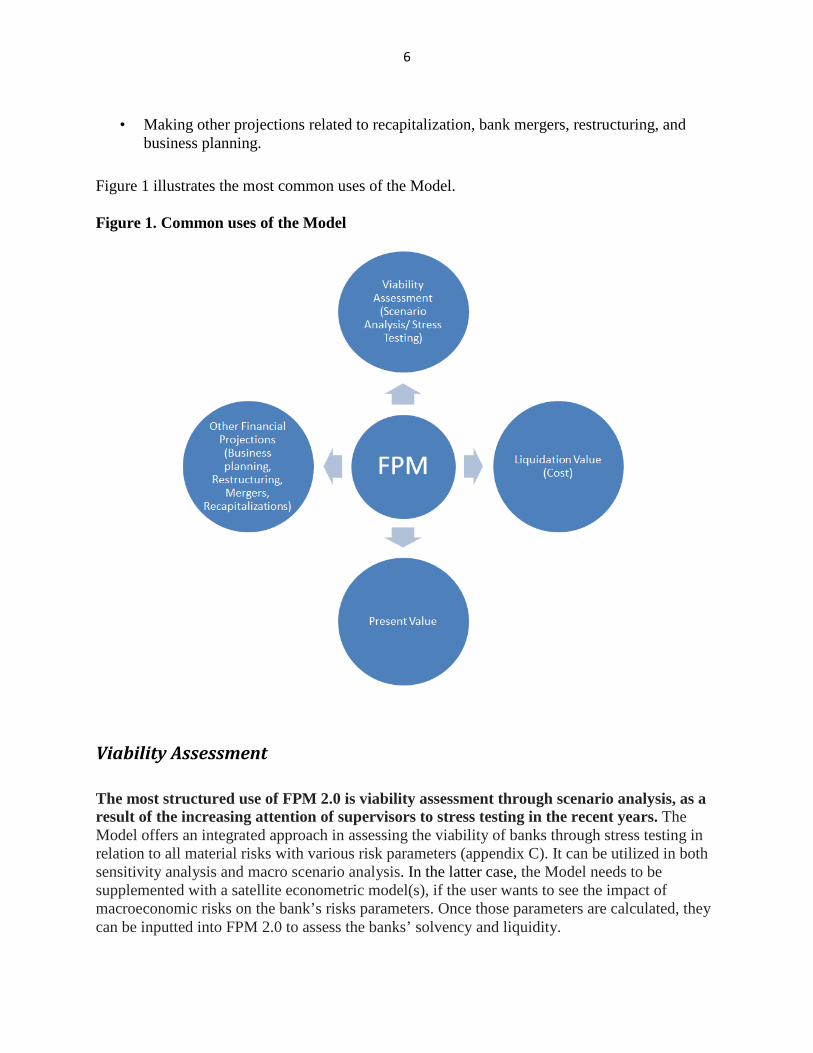
• Assessing banks’ viability based on a set of assumptions (scenarios), including stress testing, in a dynamic way, and evaluating solvency and liquidity1

• Evaluating the liquidation value (cost) of the bank under various assumptions, including the expected recovery rates on assets

• Calculating the present value of the bank under an income approach based on a discounted cash flow analysis

1 FPM 2.0 does not include macroeconomic models to map macroeconomic scenarios to banking risk parameters. Therefore, it is necessary to combine FPM 2.0 with satellite econometric models in developing robust and consistent scenarios in macro stress testing.

6

• Making other projections related to recapitalization, bank mergers, restructuring, and business planning.

Figure 1 illustrates the most common uses of the Model. Figure 1. Common uses of the Model

Viability Assessment

The most structured use of FPM 2.0 is viability assessment through scenario analysis, as a result of the increasing attention of supervisors to stress testing in the recent years. The Model offers an integrated approach in assessing the viability of banks through stress testing in relation to all material risks with various risk parameters (appendix C). It can be utilized in both sensitivity analysis and macro scenario analysis. In the latter case, the Model needs to be supplemented with a satellite econometric model(s), if the user wants to see the impact of macroeconomic risks on the bank’s risks parameters. Once those parameters are calculated, they can be inputted into FPM 2.0 to assess the banks’ solvency and liquidity.

7

FPM 2.0 can contribute to supervisory efforts in developing economies by offering an integrated risk assessment framework. To keep up with new international standards and best practices, authorities in developing economies are increasingly considering stress testing as an integral part of banking supervision. They are currently improving or building stress testing capacities, as well as building in-house modeling capability. FPM 2.0 can contribute to their needs, since it is inspired from real banking practices, it has been developed on a simple platform, and it can be customized to local needs.

Liquidation Value (Cost)

The Model has a very simple methodology to project the liquidation value of a failed or falling bank under a set of assumptions regarding asset loss rates (or recovery rates), insured deposits, covered liabilities, tangible and intangible assets valuations, and liquidation expenses. Users may benefit from the projection on a liquidation cost when assessing the cost of liquidating a bank under various deposit insurance schemes. It is suggested that users treat the liquidation value cautiously and use it only as a benchmark. Liquidation projections can be useful for supervisory authorities to assess the potential cost of a failure if the failed bank is to be liquidated. In practice, however, the cost/benefit analysis of liquidation is much more complex than the way it is presented in the Model. Moreover, especially for a systemic bank, a liquidation option might not be feasible—even if the liquidation cost is less costly than other options.

Present Value The Model can also be used to value a bank under the income approach based on cash flow projections and with assumptions about appropriate discount factors. Since in many cases privatization will follow rehabilitation, the Model can help the authorities simulate the present value of future cash flows for pricing considerations. When a sale is contemplated, comparative testing by means of alternative simulations permits an analysis of the feasibility of the business plan of the potential acquirer. This analysis can corroborate whether the bank will be able to sustain itself through shareholder support and under the new management.

Other Projections

FPM 2.0 can be utilized in any type of projection, such as bank mergers, recapitalization, restructuring, and business planning, as long as the required data are available and the relevant assumptions are developed in a coherent and consistent way. Financial projections aim to ascertain how banks will perform in the future under a particular set of assumptions that are representative of given or expected business results and/or the economic environment.

8

Potential Users of the Model FPM 2.0 is intended as a multipurpose analytical tool mainly for financial authorities (central banks, financial supervision authorities, ministries, and deposit insurance agencies). FPM 2.0 can assist supervisory and regulatory authorities, which are increasingly seeking analytical tools to assess the vulnerabilities of their banks. In addition, these authorities may be the users that benefit the most from this model, since they have technical capabilities and access to more granular and better quality data. For example, some of the data on nonperforming loan (NPL) dynamics and incomes and expenses’ subcategories might not be publicly available. Data availability and quality are key for robust projections .Without appropriate data, the Model will suffer. On the other hand, potential users include also other actors that might be interested in the Model’s projection feature. For example, banks might be interested in using the model to develop business plans and assess the risks they face. Basel II stipulates that banks are required to conduct stress tests within the context of assessing market and credit risks in the case that they choose to use internal models. Moreover, as part of Pillar II, supervisory authorities are becoming more detailed in prescribing how banks should assess their risks through stress testing.

Prerequisites for the Robust Uses of the Model

Diagnostic

Knowing the strengths and vulnerabilities of the banking system on an individual bank by bank basis and as a whole is very important to perform an affective viability assessment of the banks with FPM 2.0. Authorities have various tools, such as on-site and off-site supervision, that can be used for the diagnostic of the banking system. However, many countries may not have efficient supervision or effective collaboration among the teams that are performing diagnostics and/or those conducting viability assessment of banks. It is recommended that the authorities invest in improving supervision, as well as in improving cooperation within their teams, to be able to use the Model robustly.

Data Successful uses of the Model require reliable data. Using poor quality data is likely to result in a projection that is not credible. Less granular data might also prevent users from completing robust analysis of banks. If data quality issues are not addressed before running the Model, it is recommended that users try to overcome this problem by inputting more realistic projection assumptions that reflect known and expected events.

9

Skills In order to run a robust projection, users need to possess skills in financial reporting and analysis, financial projections, developing scenarios, and reading projection results. It is the users` responsibility to review and validate the Model before using it. Users should make sure that the Model`s methodology is appropriate for the specifics of the projection that they intend to run. Once passed this validation check, the Model can be implemented to generate relevant projections. When running a projection, not only both good quality and granular data and a robust diagnosis are important, but also a realistic and consistent set of projection assumptions. Although scenario development is mostly an art rather than a science, it is recommended that users apply other analytical tools, such as Monte Carlo simulation and econometric models, to make the scenarios more consistent and realistic.

Disclaimer for Using the Model The Model contains simplifications of real banking practices. Although the Model’s core methodology is inspired from real banking practices, certain simplifications were necessary. These simplifications and limitations might reduce the preciseness of the projection results. As revealed during the global financial crisis, almost all models fell short of identifying the risks and their magnitudes. Accordingly, the results of the model should always be considered as plausible scenarios rather than exact projections of the future. The Model’s results are based on the quality of the inputted data and the skills of the user to develop precise scenarios. As discussed, the model is just a tool. The reliability and robustness of its results will depend on the reliability of the data and the skills of the user to develop plausible scenarios. In conclusion, users should not base their decisions solely on the Model`s results. It is imperative that projection results be viewed with extreme caution and that users consider a range of relevant qualitative and quantitative information while taking appropriate decisions. FPM 2.0 shall be subject to the terms and conditions applicable for the materials, communication tools, and new tools made available to the public on the World Bank Group`s website (see http://www.worldbank.org/terms and appendix D).

http://www.worldbank.org/terms

10

The Model`s Main Features The main features of FPM 2.0 are:

• Excel-based: Formulas are developed in basic mathematical notations using algebra that any user with basic mathematics and knowledge of Excel can understand and even replicate.

• Simplicity: The Model uses simplified methodologies to project individual items on balance sheet and income statement based on rules of thumb, without applying complex econometric analyses.

• Forward-looking: The Model projects financial statements and performance indicators for users to assess risks over a future horizon.

• Inspired from actual banking practices: The Model`s main methodologies, including its balancing mechanism, are inspired from actual banking practices.

• Convenient for scenarios with any granularity: The Model can generate projections for various purposes based on very simple sensitivity analyses or comprehensive scenario analyses.

• Flexibility to define the projection horizon and the frequency: The projection horizon is the number of future periods for which the financial projections are generated. The frequency of a projection period refers to the length of the period. The model makes projections over a maximum of 12 future periods with a choice of six frequencies (annual, semi-annual, quarterly, monthly, weekly, and daily). In addition, each period can be assigned a different frequency.

• Accommodative to any degree of granularity on financial reports and other regulatory forms: The Model can be run over medium-level disaggregated data as well as high-level aggregated data. However, the preciseness of the results will be affected if data are very aggregated.

• Provides benchmarks for the development of projection assumptions: The Model calculates historical rates (implied assumptions) over the past as benchmarks for users to develop their own projection assumptions.

• Works for both individual banks and the entire system: The Model can be run over both individual banks and the whole banking system.

• Familiar structure for data entry and projections: Data can be loaded in local format and then mapped to FPM 2.0’s format. Projection results are generated in a generic format that is common or familiar in many jurisdictions.

• Informative: The Model generates well-defined CAMEL performance indicators that enable users to analyze projection results, as well as to identify sources of potential solvency or liquidity problems in a quick and effective way.2

2 CAMEL is a widely used supervisory rating system to assess a bank`s financial, operational, and managerial strengths and weaknesses. Supervisors use selected performance indicators to generate a rating for each component which are used to calculate a composite rating. In a CAMEL approach, C stands for Capital Adequacy, A for Asset Quality, M for Management Capability, E for Earnings, and L for Liquidity. In FPM 2.0, although enough

11

• Integrated approach for assessing all material risks: The Model can be used to assess credit, interest rate, liquidity, market, operational, and foreign exchange risks in an integrated way.

The limitations of FPM 2.0 are:

• Dependence on linear projections: Despite some feedback loops, most of the items are projected based on linear relationships.

• Lack of econometric analysis: Although the results of macroeconometric models can be fed into it, the Model itself does not estimate the coefficients between macroeconomic and banking risk factors. On one hand, there are limitations to using Excel to conduct robust econometric analysis. On the other hand, there is not sufficient historical data available in many countries for key items such as nonperforming loans (NPLs) to calculate default rates or loss given default rates. Therefore, if a country has available data and possesses the necessary skills and capabilities, is highly recommended that they develop satellite econometric models and input their results into FPM 2.0.

• Lack of correlations among different assets classes and liabilities: The Model does not have a methodology to estimate the correlations among different assets classes or liabilities, in terms of their risk factors. For example, if the loan quality deteriorates in one sector, the loan quality for other sectors might be impacted in the second round. This kind of analysis needs to be done outside of the Model through econometric models. Data availability and quality might hinder the ability of users to conduct econometric analysis.

• Lack of behavioral reactions: The Model assumes that banks will not react to changes in risk factors by deleveraging or adjusting portfolios. However, users can calibrate projection assumptions after each robust projection has been run to incorporate some behavioral reactions based on judgment.

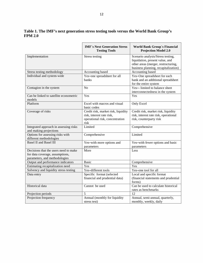
To give some idea about how FPM 2.0 differs from other tools, table 1 compares FPM 2.0 with the International Monetary Fund’s (IMF`s) stress testing tools for solvency and liquidity stress tests.3

performance indicators are developed under a CAMEL approach, no rating system is developed, since any rating methodology would be very subjective and may not be applicable in different countries. 3 Only the IMF stress testing tools publicly available in the IMF’s website are considered.

12

Table 1. The IMF’s next generation stress testing tools versus the World Bank Group’s FPM 2.0

IMF`s Next Generation Stress Testing Tools

World Bank Group`s Financial Projection Model 2.0

Implementation Stress testing Scenario analysis/Stress testing, liquidation, present value, and other areas (merger, restructuring, business planning, recapitalization)

Stress testing methodology Accounting based Accounting based Individual and system-wide Yes–one spreadsheet for all

banks Yes–One spreadsheet for each bank and an additional spreadsheet for the entire system

Contagion in the system No Yes–- limited to balance sheet interconnectedness in the system

Can be linked to satellite econometric models

Yes Yes

Platform Excel with macros and visual basic codes

Only Excel

Coverage of risks Credit risk, market risk, liquidity risk, interest rate risk, operational risk, concentration risk

Credit risk, market risk, liquidity risk, interest rate risk, operational risk, counterparty risk

Integrated approach in assessing risks and making projections

Limited Comprehensive

Options for assessing risks with different methodologies

Comprehensive Limited

Basel II and Basel III Yes–with more options and parameters

Yes–with fewer options and basic parameters

Decisions that the users need to make for data coverage, assumptions, parameters, and methodologies

More Less

Output and performance indicators Basic Comprehensive Estimating recapitalization need Yes Yes Solvency and liquidity stress testing Yes–different tools Yes–one tool for all Data entry Specific format (selected

financial and prudential data) Local and specific format (financial statements and prudential forms)

Historical data Cannot be used Can be used to calculate historical rates as benchmarks

Projection periods 5 12 Projection frequency Annual (monthly for liquidity

stress test) Annual, semi-annual, quarterly, monthly, weekly, daily

13

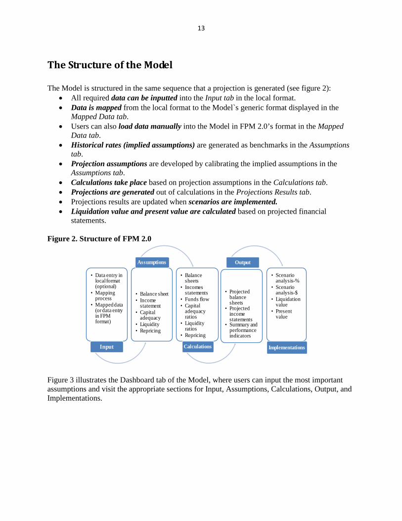
The Structure of the Model The Model is structured in the same sequence that a projection is generated (see figure 2):

• All required data can be inputted into the Input tab in the local format. • Data is mapped from the local format to the Model`s generic format displayed in the

Mapped Data tab. • Users can also load data manually into the Model in FPM 2.0’s format in the Mapped

Data tab. • Historical rates (implied assumptions) are generated as benchmarks in the Assumptions

tab. • Projection assumptions are developed by calibrating the implied assumptions in the

Assumptions tab. • Calculations take place based on projection assumptions in the Calculations tab. • Projections are generated out of calculations in the Projections Results tab. • Projections results are updated when scenarios are implemented. • Liquidation value and present value are calculated based on projected financial

statements. Figure 2. Structure of FPM 2.0

• Data entry in local format (optional)

• Mapping process

• Mapped data (or data entry in FPM format)

Input

• Balance sheet• Income

statement• Capital

adequacy• Liquidity• Repricing

Assumptions

• Balance sheets

• Incomes statements

• Funds flow• Capital

adequacy ratios

• Liquidity ratios

• Repricing

Calculations

• Projected balance sheets

• Projected income statements

• Summary and performance indicators

Output

• Scenario analysis-%

• Scenario analysis-$

• Liquidation value

• Present value

Implementations

Figure 3 illustrates the Dashboard tab of the Model, where users can input the most important assumptions and visit the appropriate sections for Input, Assumptions, Calculations, Output, and Implementations.

14

Figure 3. Dashboard tab of FPM 2.0

The Core Methodology

General The Model, which was developed using expert judgment and inspiration from real banking practices, aims to project banks` financial statements and performance indicators on an individual and a system-wide basis over a projection horizon and in various frequencies based on projection assumptions developed by users. Projected financial statements include the balance sheet, income statement, and funds flow statement (different from cash flow statement). Performance indicators are defined under a CAMEL (Capital, Asset Quality, Management, Earnings, and Liquidity) framework, including prudential ratios on capital adequacy, liquidity, and FX position. Assumptions are expectations about how independent variables will affect financial statements and prudential ratios with given methodologies. Therefore, projection results depend purely on the relationships, mostly linear with some feedback loops, between dependent and independent variables defined in the formulas and projection assumptions. The Model is a system of equations (mini models) that includes the linkages among balance sheets, income statements, funds flows, and performance indicators (appendix B).4 The formulas range from simple multiplications (such as: cash account is equivalent to the percentage

4 The methodology is explained in mathematical notation based on a simplified FPM.

15

of total deposits) to complex conditional statements (such as: if the funds flow is positive at the end of the period, the model is programmed to reduce the previous balance of emergency lending assistance before adding the residual balance to banks, securities, and loans in proportion to their historical share of total interest earning assets). The Model`s methodology combines historical trend information (historical rates/implied assumptions) with a forward-looking approach to incorporate known and expected facts and events that might affect the conditions of the bank in the future. Implied assumptions serve as the starting point for users to develop projection assumptions. Users should take into account known or expected events in the process of developing assumptions. Once the baseline projection is generated, users can implement scenario analyses to be able to capture the divergences from the baseline.

Sequence of Projections and Balancing Mechanism FPM 2.0 generates projection results for the next consecutive 12 periods based on the most recent available data and projection assumptions. Although Excel aims to solve all equations for all periods in one attempt simultaneously, conditions and feedback loops, defined as part of the methodology (such as the fact that a bank cannot pay dividends if the bank does not have profit) require an iterative process. Moreover, most of the equations are dependent on other equations (such as the central bank’s reserve requirement, which is calculated as a percentage of deposits). Therefore, once the projection is initiated, the results will be updated repeatedly until the Model converges to one solution satisfying all equations.5 The Model generates projection results for each period by applying projection assumptions to the respective line items. The projection starts when users start the process (by hitting F9 on the keyboard or selecting the “Calculate Now” ribbon under the Formulas title) after entering all necessary data and projection assumptions. Projection assumptions include but are not limited to growth rates for liabilities, interest rates on assets and liabilities, dividend rates on equity securities and investments, default rates on loans, provisioning rates for nonperforming loans, gains and losses on securities, and repayment of loans. Because of the interconnectedness among the items as well as among the projection periods, the Model updates projection results on a continuous basis through iteration. The Model will stop running once the projection results are generated for all periods after the sufficient number of iterations. The Model has a balancing mechanism that ensures that the projected balance sheet is always balanced automatically, regardless of the levels of projection assumptions entered into the Model. Once the projection assumptions are applied to the items on the balance sheet and income statement, the funds flow for each period will be computed. The balancing mechanism checks the sign of the funds flow, which can be zero, negative, or positive, and makes the necessary adjustments on the asset and/or liability sides of the balance sheet for the respective periods. Excess funds will be invested in assets and funds shortages will be satisfied 5 To see the sequence of a projection, the users can set the number of iterations as 1.

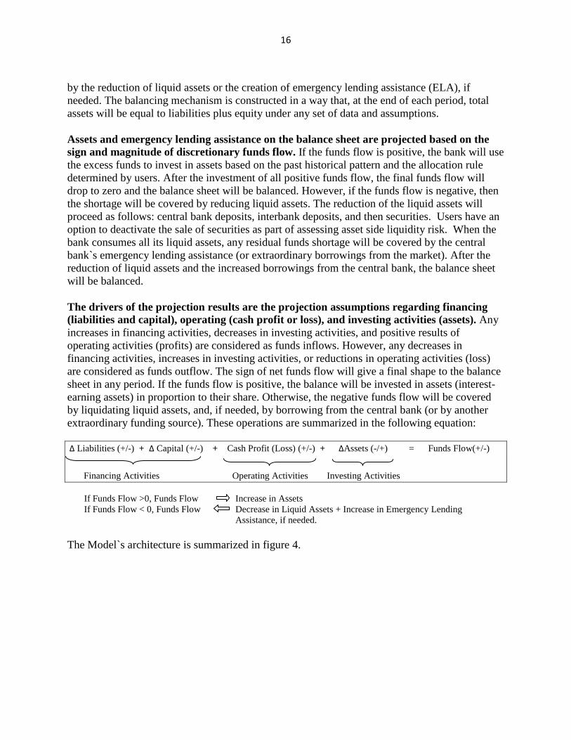
16

by the reduction of liquid assets or the creation of emergency lending assistance (ELA), if needed. The balancing mechanism is constructed in a way that, at the end of each period, total assets will be equal to liabilities plus equity under any set of data and assumptions. Assets and emergency lending assistance on the balance sheet are projected based on the sign and magnitude of discretionary funds flow. If the funds flow is positive, the bank will use the excess funds to invest in assets based on the past historical pattern and the allocation rule determined by users. After the investment of all positive funds flow, the final funds flow will drop to zero and the balance sheet will be balanced. However, if the funds flow is negative, then the shortage will be covered by reducing liquid assets. The reduction of the liquid assets will proceed as follows: central bank deposits, interbank deposits, and then securities. Users have an option to deactivate the sale of securities as part of assessing asset side liquidity risk. When the bank consumes all its liquid assets, any residual funds shortage will be covered by the central bank`s emergency lending assistance (or extraordinary borrowings from the market). After the reduction of liquid assets and the increased borrowings from the central bank, the balance sheet will be balanced. The drivers of the projection results are the projection assumptions regarding financing (liabilities and capital), operating (cash profit or loss), and investing activities (assets). Any increases in financing activities, decreases in investing activities, and positive results of operating activities (profits) are considered as funds inflows. However, any decreases in financing activities, increases in investing activities, or reductions in operating activities (loss) are considered as funds outflow. The sign of net funds flow will give a final shape to the balance sheet in any period. If the funds flow is positive, the balance will be invested in assets (interest- earning assets) in proportion to their share. Otherwise, the negative funds flow will be covered by liquidating liquid assets, and, if needed, by borrowing from the central bank (or by another extraordinary funding source). These operations are summarized in the following equation: ∆ Liabilities (+/-) + ∆ Capital (+/-) + Cash Profit (Loss) (+/-) + ∆Assets (-/+) = Funds Flow(+/-)

Financing Activities Operating Activities Investing Activities

If Funds Flow >0, Funds Flow Increase in Assets If Funds Flow < 0, Funds Flow Decrease in Liquid Assets + Increase in Emergency Lending

Assistance, if needed. The Model`s architecture is summarized in figure 4.

17

Figure 4. Architecture of FPM 2.06

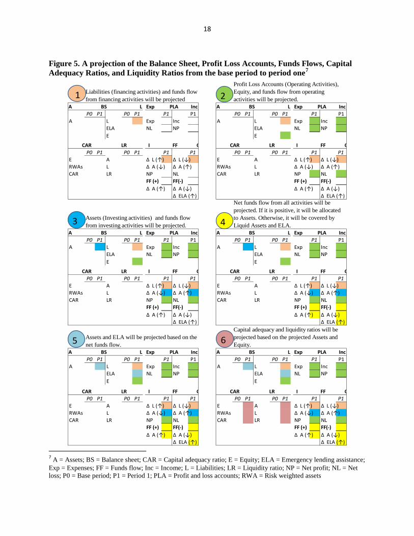
The methodology does not include automatic reactions by banks to particular assumptions or projections results. For example, higher default rates on loans do not trigger a deleveraging process or an adjustment in portfolios. Considering that banks have numerous ways to react to any changes in risk factors, it is almost impossible (and very speculative) to assume that banks will react to projection results or assumptions in a certain way. On the other hand, after reviewing the projection results, users have the flexibility to include particular reactions in the second round by calibrating respective projection assumptions. Figure 5 presents a Projection of Balance Sheet (BS), Profit Loss Accounts (PLA), Funds Flow (FF), Capital Adequacy Ratios (CAR), and Liquidity Ratios (LR) from the base period (P0) to period one (P1) in six steps.

6 CB=central bank

18

Figure 5. A projection of the Balance Sheet, Profit Loss Accounts, Funds Flows, Capital Adequacy Ratios, and Liquidity Ratios from the base period to period one7

P0 P1 P0 P1 P1 P1 P0 P1 P0 P1 P1 P1A L Exp Inc A L Exp Inc

ELA NL NP ELA NL NPE E

P0 P1 P0 P1 P1 P1 P0 P1 P0 P1 P1 P1E A Δ L (↑) Δ L (↓) E A Δ L (↑) Δ L (↓)RWAs L Δ A (↓) Δ A (↑) RWAs L Δ A (↓) Δ A (↑)CAR LR NP NL CAR LR NP NL

FF (+) FF(-) FF (+) FF(-)Δ A (↑) Δ A (↓) Δ A (↑) Δ A (↓)

Δ ELA (↑) Δ ELA (↑)











Net funds flow from all activities will be projected. If it is positive, it will be allocated to Assets. Otherwise, it will be covered by Liquid Assets and ELA.

Liabilities (financing activities) and funds flow from financing activities will be projected

Profit Loss Accounts (Operating Activities), Equity, and funds flow from operating activities will be projected.

Assets (Investing activities) and funds flow from investing activities will be projected.

A BS L Exp PLA Inc

CAR

A BS L Exp PLA Inc

CAR LR I FF O LR I FF O

A BS L Exp PLA Inc A BS L Exp PLA Inc

I FF O I FF O CAR LRCAR LR

Assets and ELA will be projected based on the net funds flow.

Capital adequacy and liquidity ratios will be projected based on the projected Assets and Equity.

CAR LR CAR LR

Exp PLA IncExp PLA Inc

I FF O I FF O

A BS L A BS L

1 2

3 4

5 6

7 A = Assets; BS = Balance sheet; CAR = Capital adequacy ratio; E = Equity; ELA = Emergency lending assistance; Exp = Expenses; FF = Funds flow; Inc = Income; L = Liabilities; LR = Liquidity ratio; NP = Net profit; NL = Net loss; P0 = Base period; P1 = Period 1; PLA = Profit and loss accounts; RWA = Risk weighted assets

19

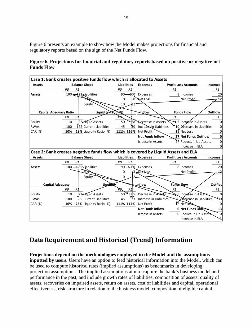
Figure 6 presents an example to show how the Model makes projections for financial and regulatory reports based on the sign of the Net Funds Flow. Figure 6. Projections for financial and regulatory reports based on positive or negative net Funds Flow Case 1: Bank creates positive funds flow which is allocated to Assets

P0 P1 P0 P1 P1 P1Assets 100 122 Liabilities 90 100 Expenses 8 Incomes 20

ELA 0 0 Net Loss Net Profit 12Equity 10 22

P0 P1 P0 P1 P1 P1Equity 10 22 Liquid Assets 50 58 Decrease in Assets 5 Increase in Assets 0RWAs 100 122 Current Liabilities 45 50 Increase in Liabilities 10 Decrease in Liabilities 0CAR (%) 10% 18% Liquidity Ratio (%) 111% 116% Net Profit 12 Net Loss 0

Net Funds Inflow 27 Net Funds Outflow 0Icrease in Assets 27 Reduct. in Liq.Assets 0

Increase in ELA 0

Case 2: Bank creates negative funds flow which is covered by Liquid Assets and ELA

P0 P1 P0 P1 P1 P1Assets 100 85 Liabilities 90 60 Expenses 8 Incomes 20

ELA 0 3 Net Loss Net Profit 12Equity 10 22

P0 P1 P0 P1 P1 P1Equity 10 22 Liquid Assets 50 37.5 Decrease in Assets 5 Increase in Assets 0RWAs 100 85 Current Liabilities 45 33 Increase in Liabilities 0 Decrease in Liabilities -30CAR (%) 10% 26% Liquidity Ratio (%) 111% 114% Net Profit 12 Net Loss 0

Net Funds Inflow 0 Net Funds Outflow 13Icrease in Assets 0 Reduct. in Liq.Assets 10

Increase in ELA 3

Inflow Funds Flow OutflowCapital Adequacy Ratio Liquidity Ratio (%)

Expenses Profit Loss Accounts IncomesAssets Balance Sheet Liabilities

Assets Balance Sheet Liabilities Expenses Profit Loss Accounts Incomes

Capital Adequacy Liquidity nflow Funds Flow Outflow

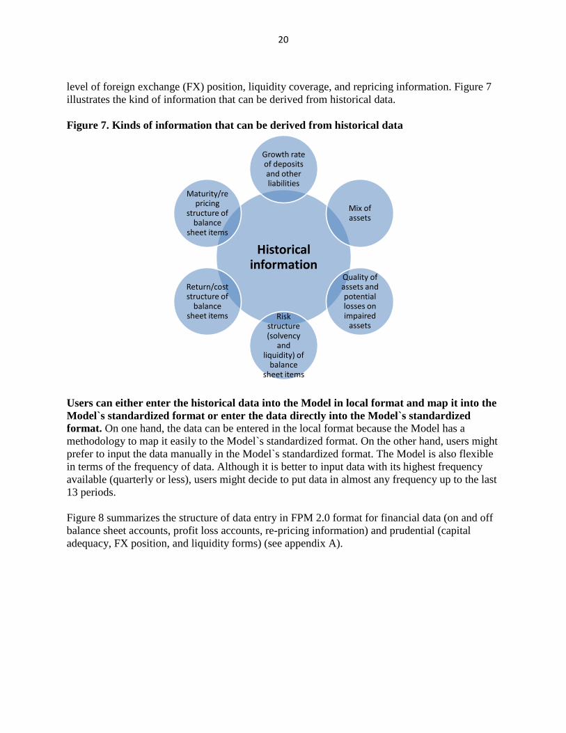
Data Requirement and Historical (Trend) Information Projections depend on the methodologies employed in the Model and the assumptions inputted by users. Users have an option to feed historical information into the Model, which can be used to compute historical rates (implied assumptions) as benchmarks in developing projection assumptions. The implied assumptions aim to capture the bank`s business model and performance in the past, and include growth rates of liabilities, composition of assets, quality of assets, recoveries on impaired assets, return on assets, cost of liabilities and capital, operational effectiveness, risk structure in relation to the business model, composition of eligible capital,

20

level of foreign exchange (FX) position, liquidity coverage, and repricing information. Figure 7 illustrates the kind of information that can be derived from historical data. Figure 7. Kinds of information that can be derived from historical data

Historical information

Growth rate of deposits and other liabilities

Mix of assets

Quality of assets and potential losses on impaired

assetsRisk

structure (solvency

and liquidity) of

balance sheet items

Return/cost structure of

balance sheet items

Maturity/repricing

structure of balance

sheet items

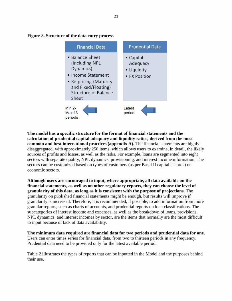
Users can either enter the historical data into the Model in local format and map it into the Model`s standardized format or enter the data directly into the Model`s standardized format. On one hand, the data can be entered in the local format because the Model has a methodology to map it easily to the Model`s standardized format. On the other hand, users might prefer to input the data manually in the Model`s standardized format. The Model is also flexible in terms of the frequency of data. Although it is better to input data with its highest frequency available (quarterly or less), users might decide to put data in almost any frequency up to the last 13 periods. Figure 8 summarizes the structure of data entry in FPM 2.0 format for financial data (on and off balance sheet accounts, profit loss accounts, re-pricing information) and prudential (capital adequacy, FX position, and liquidity forms) (see appendix A).

21

Figure 8. Structure of the data entry process

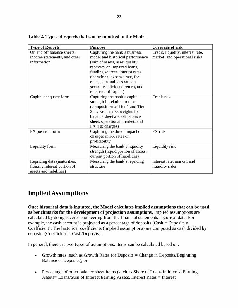
The model has a specific structure for the format of financial statements and the calculation of prudential capital adequacy and liquidity ratios, derived from the most common and best international practices (appendix A). The financial statements are highly disaggregated, with approximately 250 items, which allows users to examine, in detail, the likely sources of profits and losses, as well as the risks. For example, loans are segmented into eight sectors with separate quality, NPL dynamics, provisioning, and interest income information. The sectors can be customized based on types of customers (as per Basel II capital accords) or economic sectors. Although users are encouraged to input, where appropriate, all data available on the financial statements, as well as on other regulatory reports, they can choose the level of granularity of this data, as long as it is consistent with the purpose of projections. The granularity on published financial statements might be enough, but results will improve if granularity is increased. Therefore, it is recommended, if possible, to add information from more granular reports, such as charts of accounts, and prudential reports on loan classifications. The subcategories of interest income and expenses, as well as the breakdown of loans, provisions, NPL dynamics, and interest incomes by sector, are the items that normally are the most difficult to input because of lack of data availability. The minimum data required are financial data for two periods and prudential data for one. Users can enter times series for financial data, from two to thirteen periods in any frequency. Prudential data need to be provided only for the latest available period. Table 2 illustrates the types of reports that can be inputted in the Model and the purposes behind their use.

22

Table 2. Types of reports that can be inputted in the Model Type of Reports Purpose Coverage of risk On and off balance sheets, income statements, and other information

Capturing the bank`s business model and historical performance (mix of assets, asset quality, recovery on impaired loans, funding sources, interest rates, operational expense rate, fee rates, gain and loss rate on securities, dividend return, tax rate, cost of capital)

Credit, liquidity, interest rate, market, and operational risks

Capital adequacy form Capturing the bank`s capital strength in relation to risks (composition of Tier 1 and Tier 2, as well as risk weights for balance sheet and off balance sheet, operational, market, and FX risk charges)

Credit risk

FX position form Capturing the direct impact of changes in FX rates on profitability

FX risk

Liquidity form Measuring the bank`s liquidity strength (liquid portion of assets, current portion of liabilities)

Liquidity risk

Repricing data (maturities, floating interest portion of assets and liabilities)

Measuring the bank`s repricing structure

Interest rate, market, and liquidity risks

Implied Assumptions Once historical data is inputted, the Model calculates implied assumptions that can be used as benchmarks for the development of projection assumptions. Implied assumptions are calculated by doing reverse engineering from the financial statements historical data. For example, the cash account is projected as a percentage of deposits (Cash = Deposits x Coefficient). The historical coefficients (implied assumptions) are computed as cash divided by deposits (Coefficient = Cash/Deposits). In general, there are two types of assumptions. Items can be calculated based on:

• Growth rates (such as Growth Rates for Deposits = Change in Deposits/Beginning Balance of Deposits), or

• Percentage of other balance sheet items (such as Share of Loans in Interest Earning

Assets= Loans/Sum of Interest Earning Assets, Interest Rates = Interest

23

Income/Beginning Balance of Respective Balance Sheet Exposure, Reserve Ratio = Reserve Requirements/Total Deposits) or profit and loss items.

For the implied assumptions to be computed, a minimum of two period’s historical data, in any frequency, is needed. Average implied assumptions are calculated based on arithmetic averages of historical implied assumptions. Users are able to determine the number of historical periods in the calculation of average implied assumptions. Therefore, users need to be very careful in deciding the coverage of data points to be used in implied assumptions calculations. Any unintentional judgment can result in unrealistic projections. For example, users might have used the average of the last three years` implied interest rates, when the income statement lines are actually driven by the interest rates of just the past year. In addition, implied assumptions can be deactivated. If users do not want the Model to generate implied assumptions as benchmarks, it would be enough to load the required data for only the latest available period from which the projection would start. In this case, users need to develop all projection assumptions without taking into account the implied assumptions.

Projections Assumptions In addition of the implied assumptions, users need to develop their own projection assumptions to assess the viability of a bank more accurately. Those projection assumptions should reflect the events and conditions that have already occurred (or are expected to occur) and that might affect the bank`s financial condition over the projection horizon. If the historical rates (implied assumptions), such as default rates, provisioning rates, and/or interest rates, are not reflecting the reality on ground, it is necessary to calibrate them for projection purposes. Although implied assumptions can be used as benchmarks upon which users can base their judgments about projection assumptions, they are not a prerequisite. If users do not have historical data or prefer not to input historical data, projections assumptions can be developed based on expert judgment. By default, projection assumptions are linked to implied assumptions for convenience and users can enter their own projections assumptions manually by overriding the linkages. In addition to assumptions specific to individual items, users need to input some key assumptions—as well as constraints and rules (such as activating/deactivating market and funding liquidity risks, and/or minimum regulatory capital adequacy ratios)—in the Dashboard of the Model.

Baseline Projection The Model will generate a baseline projection based on the behavior set for each financial statement item and the projection assumptions (appendix A). Due to the nature of the assumption development process, the baseline projection reflects the users` expectations about

24

the bank`s financial position, results of operations, and level of risks, market conditions, to the best of their knowledge and expectations. Projection assumptions need to be consistent with one another and with the information used as the basis for the assumptions. Implied assumptions are useful, but may not be sufficient. Making projections based only on implied assumptions is a statistical method to calculate future items. However, it ignores the effects that are known or expected to exist; therefore, it may result in unrealistic projections. For more realistic projections, users are urged to calibrate implied assumptions to reflect the impact of events that have already affected the banks but are not yet reflected in the bank`s financial data or events that are expected to affect the bank`s conditions over the future projection horizon.

Projection Horizon The projection horizon is the number of future periods—in frequencies from daily to annual—for which the financial projections are generated. Users can run projections on the basis of the end-period financial statements for over 12 periods, with a different selected frequency for each projection period. In a usual stress testing, it is suggested that the Model be implement over a period of three years in quarterly frequency. A three-year horizon is considered sufficient time for some adverse shocks to be reflected in the bank`s solvency and liquidity. Various frequencies give users the flexibility to run projections over the desired horizons taking into account feedback and second-round effects. For example, users might be interested in running a projection for a bank over 12 periods to assess the bank`s sustainability under severe liquidity shocks. Longer frequencies may be needed to make projections for present value calculations or reorganization plans.

Projections: Static or Dynamic Balance Sheet The Model can be used for projections over a static or dynamic balance sheet. On the Dashboard, users can set a ceiling on the growth of the balance sheet items. If the ceiling is set as zero percent, the balance sheet growth will come only from the bank`s profitability, and the mix of the loan portfolio will change based on restructuring-workout, write-off, and default assumptions. For simplicity and consistency, it is suggested that users start with a projection on the assumption of a static balance sheet. In this case, assets and liabilities that mature within a projection period are assumed to be replaced with similar items in terms of type and residual maturity as at the start of the projection. Since the balance sheet growth depends on the funds flow from investment, financing, and operating activities, even if there is no change in the balance sheet items, the balance sheet numbers will change because of the impact of the operational funds flow. Consequently, interest earning assets will evolve based on the sign of operational funds flow, as well as the degree of asset quality. Positive funds flow will be

25

allocated into interest earning assets, following the same proportion that was allocated in the past, with the same business model, over the projection period. If the activities create negative funds flow, the shortage will be covered by liquidating liquid assets, and if those assets are not enough, by borrowing from the central bank.

Analyzing Projection Results Projection results can be assessed by analyzing the projected financial statements, as well as the performance indicators developed under a CAMEL approach. The Model will generate the financial statements in the format that the historical data was loaded in the Mapped Data tab. Having a standardized format for both input and output is expected to make easier for the users to assess the projection results. Users may find easier to assess the projection results against various CAMEL indicators such as CAR, Tier I ratio, liquidity ratio, ROA, ROE, NIM and leverage ratio. The Model also generates some indicative information on recapitalization needs, liquidity needs, liquidation costs, and the present value of the bank. When involved in system-wide projections, the Model also generates the number of defaults and the approximate default dates over the projection horizon. Projection results can be analyzed bank-by-bank or collectively. Since individual banks’ balance sheets are at the core of FPM 2.0, the model produces a rich set of information, and may also be used both to obtain baseline projections for individual banks and to analyze their individual performance under stress. The summary of viability and performance indicators, aside projected financial statements, is provided in figure 8 (appendix C).

26

Figure 8. Viability and performance indicators

Financial Statements

Balance Sheet

Profit Loss Account

Funds Flow

Viability Indicators

Capital Need (Total, Tier I, Core Tier I)

Liquidity Need

Liquidation Value (Cost)

Present Value

Performance Indicators (CAMEL)

Capital

Asset Quality

Management

Earnings

Liquidity

Viability Assessment

General The projections, which should reflect all known and expected events, should provide information regarding the bank`s viability. In order to test the bank`s viability under various scenarios, including stress scenarios, users can rerun the Model. A scenario analysis can be implemented against the baseline projection generated with the calibrated implied assumptions. The Model has a comprehensive approach in doing a viability assessment against credit, interest rate, market, and liquidity risks, as well as a simplified approach for assessing FX and operational risks. The Model can be used simple stress testing, like sensitivity analysis. This type of analysis is recommended in countries that have basic supervisory data and lack the necessary historical data or good quality data for econometric modeling. With FPM 2.0, users can test the impact of change(s) in the risk factors, considering other factors fixed. In addition, the Model can be complemented with comprehensive macro scenarios. To analyze the impact of macro scenarios in banks, it is necessary to calculate the impact of macroeconomic shocks in banking risk factors outside the model by means of satellite econometric models. Once those parameters are calculated, they can be inputted into FPM 2.0 (figure 9).

27

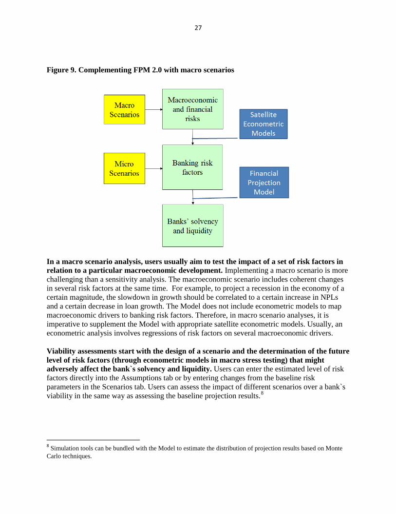
Figure 9. Complementing FPM 2.0 with macro scenarios

In a macro scenario analysis, users usually aim to test the impact of a set of risk factors in relation to a particular macroeconomic development. Implementing a macro scenario is more challenging than a sensitivity analysis. The macroeconomic scenario includes coherent changes in several risk factors at the same time. For example, to project a recession in the economy of a certain magnitude, the slowdown in growth should be correlated to a certain increase in NPLs and a certain decrease in loan growth. The Model does not include econometric models to map macroeconomic drivers to banking risk factors. Therefore, in macro scenario analyses, it is imperative to supplement the Model with appropriate satellite econometric models. Usually, an econometric analysis involves regressions of risk factors on several macroeconomic drivers. Viability assessments start with the design of a scenario and the determination of the future level of risk factors (through econometric models in macro stress testing) that might adversely affect the bank`s solvency and liquidity. Users can enter the estimated level of risk factors directly into the Assumptions tab or by entering changes from the baseline risk parameters in the Scenarios tab. Users can assess the impact of different scenarios over a bank`s viability in the same way as assessing the baseline projection results.8

8 Simulation tools can be bundled with the Model to estimate the distribution of projection results based on Monte Carlo techniques.

28

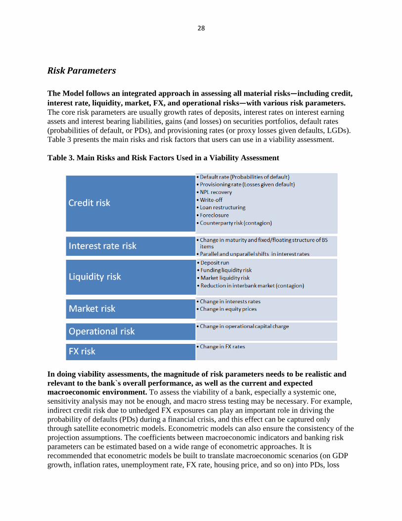
Risk Parameters The Model follows an integrated approach in assessing all material risks—including credit, interest rate, liquidity, market, FX, and operational risks—with various risk parameters. The core risk parameters are usually growth rates of deposits, interest rates on interest earning assets and interest bearing liabilities, gains (and losses) on securities portfolios, default rates (probabilities of default, or PDs), and provisioning rates (or proxy losses given defaults, LGDs). Table 3 presents the main risks and risk factors that users can use in a viability assessment. Table 3. Main Risks and Risk Factors Used in a Viability Assessment

In doing viability assessments, the magnitude of risk parameters needs to be realistic and relevant to the bank`s overall performance, as well as the current and expected macroeconomic environment. To assess the viability of a bank, especially a systemic one, sensitivity analysis may not be enough, and macro stress testing may be necessary. For example, indirect credit risk due to unhedged FX exposures can play an important role in driving the probability of defaults (PDs) during a financial crisis, and this effect can be captured only through satellite econometric models. Econometric models can also ensure the consistency of the projection assumptions. The coefficients between macroeconomic indicators and banking risk parameters can be estimated based on a wide range of econometric approaches. It is recommended that econometric models be built to translate macroeconomic scenarios (on GDP growth, inflation rates, unemployment rate, FX rate, housing price, and so on) into PDs, loss

29

given defaults (LGDs), interest rates, and growth rates for the balance sheet items. Then, the estimated risk factors need to be fed into the Model to assess their impact on various metrics, including the solvency and liquidity of the bank. Users can define hypothetical, historical, or probabilistic scenarios, or a combination of them. The usual practice is to apply historical calibration. With this technique, the size of the change in a variable is determined according to the largest change that this variable experienced over a certain period of time in the past. The selection of this time period is closely related to the type of risk being analyzed and to the circumstances prevailing in the bank’s operating environment over that period. If there is enough time series data for selected variables, users can also use the distribution of changes in variables to select a given percentile or a certain probability of occurrence and to determine the value that the variable would have in an extreme situation. In other cases, especially when available data of the required quality is scarce, users can use hypothetical calibration based on expert judgment. In a hypothetical calibration, a change in the variable is an input based on assumptions that might not have been observed in the past.

Inputting Risk Parameters into the Model Users can implement risk parameters two different ways:

1. Calibrating projection assumptions in the Assumptions tab (such as changing the implied

default rates from 1% to 5% over a year manually).

2. Defining changes from the baseline projection assumptions as percentage points (such as increasing the default rates over a year by 4 percentage points) in the Scenario Analysis -% tab, or entering absolute changes in the Scenario Analysis -$ tab (such as adding $100 million, equivalent to 4% of performing loans, in the NPLs category, and subtracting the same amount in the Performing Loans category in the first projection period).

Metrics The Model is equipped with a variety of metrics to help users analyze the viability of banks based on different scenarios. In general, a viable bank is a bank that operates without government support in the form of capital or liquidity. Therefore, the most important metrics to determine the viability of a bank are solvency and liquidity. In many jurisdictions, banks with regulatory capital adequacy ratios below the minimum requirement are considered insolvent, given that the bank cannot raise capital within a reasonable period of time. Moreover, a bank that has problems meeting its obligations to pay its borrowers is deemed to have a liquidity issue. However, in practice, it is very complicated to assume that a bank with a liquidity problem is unviable since the central bank can provide liquidity to the bank, as long as it is solvent, under an emergency lending scheme. Therefore, the main viability test for a bank is the adequacy of its

30

capital level. In the Model, regulatory capital adequacy and liquidity are set as thresholds for triggering a default. On the other hand, all other CAMEL performance indicators might also be included in the assessment of the viability of banks. In practice, liquidity and solvency are interrelated and very hard to separate. For example, in the event of funding liquidity risk, a liquidity problem may turn into a solvency problem if the bank cannot raise funds by liquidating assets. The closure of markets or fire sales may increase funding costs, and therefore lead to the insolvency of the bank. On the other hand, a solvency problem can also lead to a liquidity problem, since solvency is the main risk factor that is taken into account by fund providers. For example, a bank with a solvency problem might have difficulty in rolling over its current borrowings or acquiring new borrowings. Solvency tests

For projection purposes, it is assumed that a bank is solvent if the regulatory capital adequacy ratios over the projection horizon are above a threshold set by users. Users have flexibility to set the threshold that ensures that a bank has sufficient capital to be able to withstand shocks, without breaching minimum capital adequacy requirements. The Model projects various regulatory capital adequacy ratios, such as Total/Tier 1/Core Tier 1 capital adequacy ratios, and risk-weighted assets (RWA). In addition to basic leverage ratios, other capital adequacy indicators are also projected by the Model, such as capital shortfalls (the amount of capital needed to maintain the regulatory capital adequacy ratios above the minimum). The regulatory capital adequacy ratio, the main solvency indicator, is measured as eligible capital (Tier I Capital + Tier 2 Capital) divided by risk weighted assets (sum of risk-weighted assets for on- and off-balance sheet items, together with market risk, operational risk, and foreign exchange risk). The evolution of eligible capital reflects projected after-tax net income for each period minus cash dividends. Paid-up capital is projected as part of the scenario analysis. Other Tier1 and Tier 2 items will evolve as a proxy of underlying items based on the latest available capital adequacy report. Risk-weighted assets will be projected by applying risk weights, which are calculated based on the latest available report, to underlying projected items (gross income for calculating risk-weighted assets for operational risk, trading portfolio for market risk, FX position for FX risk). The Model’s approach is suitable for different methods to calculate risk-weighted assets such as the regulatory weights or any other risk rating models suggested by the Basel Capital Accords. Liquidity tests

Liquidity tests examine banks` capacity to generate enough funds from their activities to withstand any cash outflows. Because of its nature, a liquidity shock can easily lead to a default, even if the bank is solvent. A maturity mismatch can easily create a liquidity distress in the form of a deposit run or a dry-up of funding in investment markets. With the model, users can simulate funding liquidity risk and/or market liquidity risk conditions. The Model also has channels of risk propagation that can turn a specific liquidity problem into a liquidity crisis.

31

Individual or System-Wide Projections The Model can generate projections on an individual and a system-wide basis. System-wide projections aim to assess the viability of the whole financial system, as opposed to individual projections, which are designed to stress individual banks. The system-wide Model allows users to run standardized or tailor-made scenarios over all banks simultaneously, with or without taking into account the contagion in the banking system.

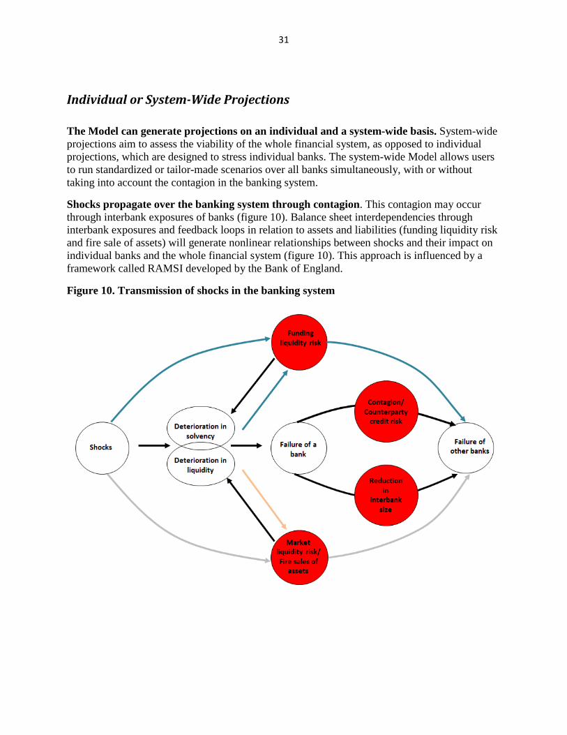
Shocks propagate over the banking system through contagion. This contagion may occur through interbank exposures of banks (figure 10). Balance sheet interdependencies through interbank exposures and feedback loops in relation to assets and liabilities (funding liquidity risk and fire sale of assets) will generate nonlinear relationships between shocks and their impact on individual banks and the whole financial system (figure 10). This approach is influenced by a framework called RAMSI developed by the Bank of England.

Figure 10. Transmission of shocks in the banking system

32

Funding liquidity risk

Funding liquidity risk appears when a bank has problems in rolling over its existing liabilities or raising new ones because of a perceived solvency problem about itself by wholesale lenders. The level of total capital adequacy ratio, a solvency indicator, is set as a trigger for funding liquidity risk. Once activated by users, if the bank`s capital adequacy ratio deteriorates beyond the threshold, the bank would not be able to roll over its maturing debt and raise new debt from the money and capital markets. Unlike wholesale lenders, depositors are assumed to have little incentive to evaluate the solvency of banks and move their deposits to other banks with better solvency. This behavior is also related to explicit or implicit safety nets in the system. The closure of the money and capital markets to a bank with a solvency problem may lead to a liquidity problem that might ultimately trigger a fire sale of securities. A fire sale of securities can reduce security prices dramatically, which might force all banks to write down their securities, especially the ones carrying big trading portfolios. However, the Model does not automatically map a fire sale of securities of a bank to a wider reduction of securities in the market. The magnitude of the reduction in securities prices need to be defined by users manually by changing respective assumptions.

(Fire) sale of securities

A bank with liquidity needs is assumed to liquidate money market operations. The liquidation process will be triggered by discrete cash flows generated by operating, investment, and financing activities during the period. Excess funds flows are invested in loans and securities portfolios, based on the allocation rule determined by users. Banks can pay dividends to their shareholders—provided that they comply with the minimum capital adequacy ratio before investing in loans and securities. Negative cash flows are covered by the reduction of money market operations and by the sales of Held for Trading securities in the first place and Available for Sale securities in the second place. After the sale of securities, if a funds shortage continues, the central bank is assumed to provide emergency lending assistance to cover the shortage. The bank with liquidity needs cannot raise money in the interbank market since the volume of this market is assumed to be constrained by the supply side. In the Model, banks can satisfy the liquidity needs that have not been covered by the interbank market through the central bank`s emergency lending assistance. In addition, the fire sale of assets may lead to a further deterioration of capital adequacy, while solving the liquidity problem. The impact of a fire sale of assets on profitability—and, ultimately, capital adequacy—depends on the sales loss rate, which is decided by users. When the total capital adequacy ratio falls below the threshold as a result of the assets fire sale, the bank is considered in default.

Contagion

Users can assess the impact of contagion via interbank connectedness. Even though there may be other interdependencies between banks, the Model recognizes only those linkages that

33

stem from interbank exposures. Contagion occurs if the failure of a bank (or banks) leads to subsequent defaults on other banks. In the Model, default occurs when a bank`s total capital adequacy ratio falls short of the minimum requirement—the threshold—which is expected to be set by users. The Model can be customized to include liquidity indicators or other performance indicators in the definition of default. When a bank`s capital adequacy ratio is projected to be lower than the threshold in any period, the bank is considered to have defaulted. A default in one of the banks of the system can lead to new defaults. The Model performs a viability check for each period and determines if any more banks have defaulted. Default affects other banks through two channels: through the reduction in the size of the interbank market, and through the counterparty loss to surviving banks. The loss- sharing generated by the defaulted bank`s net interbank liabilities may result in the fact that some other banks` capital adequacy ratio falls short from the threshold, as well. The additional new defaults can bring some more banks to default in a third round, and so forth. The loop will repeat until the default cascade ends over the projection horizon.

• Counterparty Risk The surviving banks might incur losses because of their exposures to the defaulted bank(s) if the defaulted bank(s) is a net interbank borrower. It is assumed that a defaulted bank will not be able to repay its net interbank liabilities. Therefore, those net interbank liabilities will have to be written off and the lender banks will incur the losses. The lender banks are assumed to share the losses originated from the defaulted bank(s) in proportion to their share of total interbank assets. Although this is a suboptimal method of distributing losses to the surviving banks, it can be implemented easily if actual exposures data are not available or actual exposures are not stable for loss projections.

• Drying up of interbank market The surviving banks might borrow less in the interbank market because of the reduction of the size of the market, in the case that the defaulted bank(s) was/were a net interbank lender. The Model is constructed to ensure that total interbank assets are equal to total interbank liabilities following a default in each period. To maintain this condition, the Model first projects the surviving banks` interbank assets and then distributes them to the borrower banks in proportion to these banks` total interbank liabilities before the default.

34

Liquidation Value Calculation The liquidation cost (or value) of a bank is calculated by applying loss rates to its asset accounts under various deposit insurance schemes. The liquidation cost is not the only input in decision-making with respect to a failed or failing bank. In practice, the calculation of liquidation costs is much more complex than the Model`s methodology. Moreover, especially for a systemic bank, a liquidation option might not be feasible even if the liquidation cost is less than the cost of other options. Therefore, users are suggested to take the liquidation value cautiously as a benchmark and support it with other quantitative and qualitative approaches. The Model calculates the liquidation value at the date of default if a bank is projected to default. For the Model to project a liquidation value, users need to input expected loss rates on assets and off-balance sheet exposures in the Liquidation tab. Developing loss rates might be difficult in countries with no liquidation experience or no available historical loss data. In this case, loss rates can be developed based on due diligence or a review of asset quality. Otherwise, users may choose to input the loss rates of other countries with a similar level of financial development. The net asset value is the present value of the assets considered for liquidation, taking into consideration the liquidation expenses, revalued effect of tangible assets, and the appraisal of intangible assets, as well as the projected insured deposits and covered liabilities. For example, a failed bank can have very profitable subsidiaries and associates, which should be included in the valuation of assets. The bank can also have profitable business units, such as credit card and financial consulting services, which can be sold separately to interested investors. The deposit insurance fund can also ask for premiums in return for transferring bank`s deposits and loans to the acquirers. The insurer can make additional discounts over the expected value of the assets, given that there could be a potential risk, which might hinder the realization of the expected value of the assets. Liquidation expenses include all expenditures necessary to implement the liquidation of a bank, such as the salaries, the rent of premises, and the fees for legal and professional services. Users have to enter into the Model the expense ratio over the asset values for the liquidation expenses, the average years to complete the transaction, and the opportunity cost of liquidation. Covered liabilities have priority to be paid over insured liabilities. Covered liabilities are comprised of all liabilities supported by collateral (usually repos, covered bonds, and foreign borrowings). The deposit insurance fund must pay these liabilities up to their collateral value.

35

Present Value Calculation FPM 2.0 calculates the present value of the stream of dividends available for discretionary distribution at the end of the projection periods. After the projection horizon, FPM 2.0 also adds the present value of the estimated perpetuity for period 12 of the projection, which simulates the residual value of the banks at that date. This calculation excludes from the discretionary dividends in each period any foreseen material capital investment and regulatory capital adequacy needs. By default, discount rates are linked to the costs of liabilities and capital; however, it is possible that users could override the formulas and enter the discount rates manually.

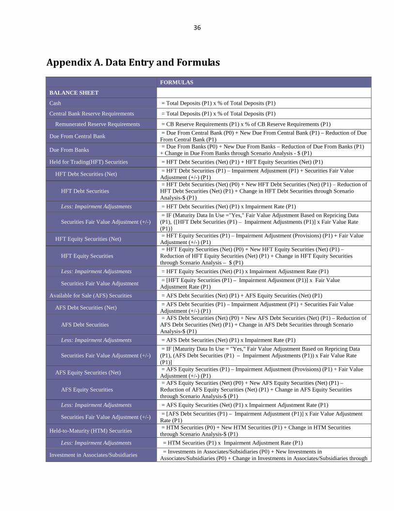
36

Appendix A. Data Entry and Formulas

FORMULAS

BALANCE SHEET

Cash = Total Deposits (P1) x % of Total Deposits (P1)

Central Bank Reserve Requirements = Total Deposits (P1) x % of Total Deposits (P1)

Remunerated Reserve Requirements = CB Reserve Requirements (P1) x % of CB Reserve Requirements (P1)

Due From Central Bank = Due From Central Bank (P0) + New Due From Central Bank (P1) – Reduction of Due From Central Bank (P1)

Due From Banks = Due From Banks (P0) + New Due From Banks – Reduction of Due From Banks (P1) + Change in Due From Banks through Scenario Analysis - $ (P1)

Held for Trading(HFT) Securities = HFT Debt Securities (Net) (P1) + HFT Equity Securities (Net) (P1)

HFT Debt Securities (Net) = HFT Debt Securities (P1) – Impairment Adjustment (P1) + Securities Fair Value Adjustment (+/-) (P1)

HFT Debt Securities = HFT Debt Securities (Net) (P0) + New HFT Debt Securities (Net) (P1) – Reduction of HFT Debt Securities (Net) (P1) + Change in HFT Debt Securities through Scenario Analysis-$ (P1)

Less: Impairment Adjustments = HFT Debt Securities (Net) (P1) x Impairment Rate (P1)

Securities Fair Value Adjustment (+/-) = IF (Maturity Data In Use ="Yes," Fair Value Adjustment Based on Repricing Data (P1), {[HFT Debt Securities (P1) – Impairment Adjustments (P1)] x Fair Value Rate (P1)}

HFT Equity Securities (Net) = HFT Equity Securities (P1) – Impairment Adjustment (Provisions) (P1) + Fair Value Adjustment (+/-) (P1)

HFT Equity Securities = HFT Equity Securities (Net) (P0) + New HFT Equity Securities (Net) (P1) – Reduction of HFT Equity Securities (Net) (P1) + Change in HFT Equity Securities through Scenario Analysis – $ (P1)

Less: Impairment Adjustments = HFT Equity Securities (Net) (P1) x Impairment Adjustment Rate (P1)

Securities Fair Value Adjustment = [HFT Equity Securities (P1) – Impairment Adjustment (P1)] x Fair Value Adjustment Rate (P1)

Available for Sale (AFS) Securities = AFS Debt Securities (Net) (P1) + AFS Equity Securities (Net) (P1)

AFS Debt Securities (Net) = AFS Debt Securities (P1) – Impairment Adjustment (P1) + Securities Fair Value Adjustment (+/-) (P1)

AFS Debt Securities = AFS Debt Securities (Net) (P0) + New AFS Debt Securities (Net) (P1) – Reduction of AFS Debt Securities (Net) (P1) + Change in AFS Debt Securities through Scenario Analysis-$ (P1)

Less: Impairment Adjustments = AFS Debt Securities (Net) (P1) x Impairment Rate (P1)

Securities Fair Value Adjustment (+/-) = IF [Maturity Data In Use = "Yes," Fair Value Adjustment Based on Repricing Data (P1), (AFS Debt Securities (P1) – Impairment Adjustments (P1)) x Fair Value Rate (P1)]

AFS Equity Securities (Net) = AFS Equity Securities (P1) – Impairment Adjustment (Provisions) (P1) + Fair Value Adjustment (+/-) (P1)

AFS Equity Securities = AFS Equity Securities (Net) (P0) + New AFS Equity Securities (Net) (P1) – Reduction of AFS Equity Securities (Net) (P1) + Change in AFS Equity Securities through Scenario Analysis-$ (P1)

Less: Impairment Adjustments = AFS Equity Securities (Net) (P1) x Impairment Adjustment Rate (P1)

Securities Fair Value Adjustment (+/-) = [AFS Debt Securities (P1) – Impairment Adjustment (P1)] x Fair Value Adjustment Rate (P1)

Held-to-Maturity (HTM) Securities = HTM Securities (P0) + New HTM Securities (P1) + Change in HTM Securities through Scenario Analysis-$ (P1)

Less: Impairment Adjustments = HTM Securities (P1) x Impairment Adjustment Rate (P1)

Investment in Associates/Subsidiaries = Investments in Associates/Subsidiaries (P0) + New Investments in Associates/Subsidiaries (P0) + Change in Investments in Associates/Subsidiaries through

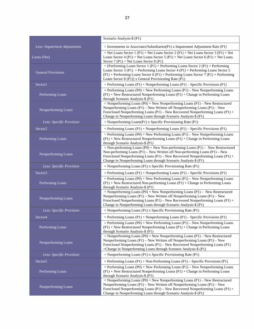
37

Scenario Analysis-$ (P1)

Less: Impairment Adjustments = Investments in Associates/Subsidiaries(P1) x Impairment Adjustment Rate (P1)

Loans (Net) = Net Loans Sector 1 (P1) + Net Loans Sector 2 (P1) + Net Loans Sector 3 (P1) + Net Loans Sector 4 (P1) + Net Loans Sector 5 (P1) + Net Loans Sector 6 (P1) + Net Loans Sector 7 (P1) + Net Loans Sector 8 (P1)

General Provisions

= [Performing Loans Sector 1 (P1) + Performing Loans Sector 2 (P1) + Performing Loans Sector 3 (P1) + Performing Loans Sector 4 (P1) + Performing Loans Sector 5 (P1) + Performing Loans Sector 6 (P1) + Performing Loans Sector 7 (P1) + Performing Loans Sector 8 (P1)] x General Provisioning Rate (P1)

Sector1 = Performing Loans (P1) + Nonperforming Loans (P1) – Specific Provisions (P1)

Performing Loans = Performing Loans (P0) + New Performing Loans (P1) – New Nonperforming Loans (P1) + New Restructured Nonperforming Loans (P1) + Change in Performing Loans through Scenario Analysis-$ (P1)

Nonperforming Loans

= Nonperforming Loans (P0) + New Nonperforming Loans (P1) – New Restructured Nonperforming Loans (P1) – New Written off Nonperforming Loans (P1) – New Foreclosed Nonperforming Loans (P1) – New Recovered Nonperforming Loans (P1) + Change in Nonperforming Loans through Scenario Analysis-$ (P1)

Less: Specific Provision = Nonperforming Loans(P1) x Specific Provisioning Rate (P1)



Nonperforming Loans

= Non-performing Loans (P0) + New Non-performing Loans (P1) – New Restructured Non-performing Loans (P1) – New Written off Non-performing Loans (P1) – New Foreclosed Nonperforming Loans (P1) – New Recovered Nonperforming Loans (P1) + Change in Nonperforming Loans through Scenario Analysis-$ (P1)

Less: Specific Provision = Nonperforming Loans (P1) x Specific Provisioning Rate (P1)


Performing Loans = Performing Loans (P0) + New Performing Loans (P1) – New Nonperforming Loans (P1) + New Restructured Non-performing Loans (P1) + Change in Performing Loans through Scenario Analysis-$ (P1)

Nonperforming Loans





Nonperforming Loans

= Nonperforming Loans (P0) + New Nonperforming Loans (P1) – New Restructured Nonperforming Loans (P1) – New Written off Nonperforming Loans (P1) – New Foreclosed Nonperforming Loans (P1) – New Recovered Nonperforming Loans (P1) +Change in Nonperforming Loans through Scenario Analysis-$ (P1)


Sector5 = Performing Loans (P1) + Non-Performing Loans (P1) – Specific Provisions (P1)


Nonperforming Loans


38




Nonperforming Loans





Nonperforming Loans





Nonperforming Loans

= Nonperforming Loans (P0) + New Nonperforming Loans (P1) – New Restructured Nonperforming Loans (P1) – New Written-off Nonperforming Loans (P1) – New Foreclosed Nonperforming Loans (P1) – New Recovered Nonperforming Loans (P1) + Change in Nonperforming Loans through Scenario Analysis-$ (P1)


Interest Accrued Receivables on Loans = Total Interest Income from Loans (P1) x Interest Accrual Rate (P1) + Change in Interest Accrued Receivables on Loans through Scenario Analysis-$ (P1)

Foreclosed Assets = Foreclosed Assets (P0) + New Foreclosed Nonperforming Loans (P1) + Change in Foreclosed Assets through Scenario Analysis-$ (P1)

Less: Impairment Adjustments = Foreclosed Assets (P1) x Provisioning Rate (P1)

Other Assets = Other Liabilities (P1) x Other Assets-to-Other Liabilities Rate (P1) + Change in Other Assets through Scenario Analysis-$ (P1)

TOTAL ASSETS

= Cash (P1) + CB Reserve Requirement (P1) + Due From CB (P1) + Due From Banks (P1) + HFT Securities (Net) (P1) + AFS Securities (Net) (P1) + HTM Securities (Net) (P1) + Investments in Associates/Subsidiaries (Net) (P1) + Loans (Net) (P1) + Interest Accrued Receivables on Loans (P1) + Foreclosed Assets (Net) (P1) + Other Assets (P1)

LIABILITIES & EQUITY

LIABILITIES

Deposits = SUM (Deposits1 + Deposits2 + Deposits3+ Deposits1 + Deposits2 + Deposits3 + Deposits4) (P1)

Deposits1 = Deposits1 (P0) x [1+ Growth Rate (P1)] + Change in Deposits through Scenario Analysis-$ (P1)




Due to Banks = Due to Banks (P0) x [1+ Growth Rate (P1)] + Change in Due to Banks through

39

Scenario Analysis-$ (P1)

Due to Central Bank = Due to Central Bank (P0) x [1+ Growth Rate (P1)] + Change in Due to Central Bank through Scenario Analysis-$ (P1)

Emergency Lending Assistance (ELA) from Central Bank = Funding Deficit Needs to be Covered by ELA (P1)

Borrowings1

= IF [AND (Funding Liquidity Risk = "Yes," Projected CAR (P0) < Regulatory Minimum CAR), IF (Maturity Data in Use, Residual of Previous Borrowings1 (P1), 0), + Borrowings1 (P0) x (1+ Growth Rate (P1))] + Change in Borrowings1 through Scenario Analysis-$ (P1)

Borrowings2

= IF [AND (Funding Liquidity Risk ="Yes", Projected CAR (P0) <Regulatory Minimum CAR), IF(Maturity Data in Use, Residual of Previous Borrowings2 (P1), 0), + Borrowings2 (P0) x (1+ Growth Rate (P1)] + Change in Borrowings2 through Scenario Analysis-$ (P1)

Subordinated Loans = Subordinated Bonds 1 (P0) x [1+ Growth Rate (P1)] + Change in Subordinated Bonds through Scenario Analysis-$ (P1)

General Provisions for Off-Balance Sheet Liabilities = Financial Guarantees (P1) x Provisioning Rate (P1)

Other Liabilities = Other Liabilities 1 (P0) x [1+ Growth Rate (P1)] + Change in Other Liabilities through Scenario Analysis-$ (P1)

TOTAL LIABILITIES

= Total Deposits (P1) + Due to Banks (P1) + Due to Central Bank (P1) + ELA from Central Bank (P1) + Borrowings1 (P1) + Borrowings1 (P1) + Borrowings2 (P1) + Subordinated Bonds (P1) + General Provisions for Off-Balance Sheet Liabilities (P1) + Other Liabilities (P1)

SHAREHOLDER`S EQUITY

Common Stocks = Common Stock (P0) + Change in Common Stock through Scenario Analysis-$ (P1)

Preferred Stocks = Preferred Stock (P0) + Change in Preferred Stock through Scenario Analysis-$ (P1)

Retained Earnings = Retained Earnings (P0) + Retained Earnings (P1)

Fair Value Adjustments for AFS Securities = AFS Debt Securities Fair Value Adjustment (P1) + HFT Debt Securities Fair Value Adjustment (P1)

Other Equity = Other Equity (P0) + Change in Other Equity through Scenario Analysis-$ (P1)

TOTAL SHAREHOLDER`S EQUITY = Common Stock (P1) + Preferred Stock (P1) + Retained Earnings (P1) + Gains/Losses on AFS Securities (P1) + Other Equity (P1)

TOTAL LIABILITIES & EQUITY = Total Shareholder's Equity (P1) + Total Liabilities (P1)

OFF-BALANCE SHEET ACTIVITY

Financial Guarantees = Financial Guarantees (P0) x [1+ Growth Rate (P1)]

Contingent Commitments = Contingent Commitments (P0) x [1+ Growth Rate (P1)]

Derivatives = Derivatives (P0) x [1+ Growth Rate (P1)]

OTHER INFORMATION

Flow of NPLs

New NPLs = SUM (Sector1, Sector2, Sector3, Sector4, Sector5, Sector6, Sector7, Sector8)

Sector1 = Performing Loans (P0) x Default Rate (P1)



40






Restructured/Worked out NPLs = SUM (Sector1, Sector2, Sector3, Sector4, Sector5, Sector6, Sector7, Sector8)

Sector1 = [Nonperforming Loans (P0) + New Nonperforming Loans (P1)] x Default Rate (P1)








Written-off NPLs = SUM (Sector1, Sector2,Sector3, Sector4, Sector5, Sector6, Sector7, Sector8)

Sector1 = [Nonperforming Loans (P0) + New Nonperforming Loans (P1)] x Write-off Rate (P1)








Foreclosed NPLs = SUM (Sector1, Sector2,Sector3, Sector4,Sector5, Sector6,Sector7, Sector8)

Sector1 = [Nonperforming Loans (P0) + New Nonperforming Loans (P1)] x Foreclosure Rate (P1)








Recovered/Sold NPLs = SUM (Sector1, Sector2, Sector3, Sector4, Sector5, Sector6, Sector7, Sector8)

Sector1 = [Nonperforming Loans (P0) + New Nonperforming Loans (P1)] x Recovery Rate (P1)



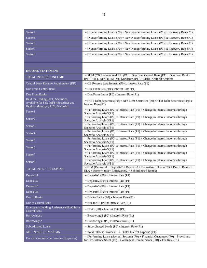
41






INCOME STATEMENT

TOTAL INTEREST INCOME = SUM (CB Remunerated RR (P1) + Due from Central Bank (P1) + Due from Banks (P1) + HFT, AFS, HTM Debt Securities (P1) + Loans [Sector1: Sector8]

Central Bank Reserve Requirement (RR) = CB Reserve Requirement (P0) x Interest Rate (P1)

Due From Central Bank = Due From CB (P0) x Interest Rate (P1)

Due From Banks = Due From Banks (P0) x Interest Rate (P1) Held for Trading(HFT) Securities, Available for Sale (AFS) Securities and Held-to-Maturity (HTM) Securities

= [HFT Debt Securities (P0) + AFS Debt Securities (P0) +HTM Debt Securities (P0)] x Interest Rate (P1)

Sector1 = Performing Loans (P0) x Interest Rate (P1) + Change in Interest Incomes through Scenario Analysis-$(P1)








TOTAL INTEREST EXPENSE =SUM (Deposits1 + Deposits2 + Deposits3 + Deposits4 + Due to CB + Due to Banks + ELA + Borrowings1+ Borrowings2 + Subordinated Bonds)

Deposits1 = Deposits1 (P0) x Interest Rate (P1)




Due to Banks = Due to Banks (P0) x Interest Rate (P1)

Due to Central Bank = Due to CB (P0) x Interest Rate (P1) Emergency Lending Assistance (ELA) from Central Bank = ELA1 (P0) x Interest Rate (P1)

Borrowings1 = Borrowings1 (P0) x Interest Rate (P1)

Borrowings2 = Borrowings2 (P0) x Interest Rate (P1)

Subordinated Loans = Subordinated Bonds (P0) x Interest Rate (P1)

NET INTEREST MARGIN = Total Interest Income (P1) – Total Interest Expense (P1)

Fee and Commission Incomes (Expenses) = [Performing Loans (Sector1:Sector8) (P0) + Financial Guarantees (P0) – Provisions for Off-Balance Sheet (P0) + Contingent Commitments (P0)] x Fee Rate (P1)

42

Gains (Losses) on Securities

=+[HFT Debt Securities (Net) (P0) + HFT Equity Securities (Net) (P0) + AFS Debt Securities (Net) (P0) + AFS Equity Securities (Net) (P0)] x Gains (Losses) Rate (P1) + HFT Debt Securities Fair Value Adjustment (P1) + HFT Equity Securities Fair Value Adjustment (P1) + IF(OR(Impairment Adjustment Rate (P1) = 100%, Fair Value Adjustment Rate (P1) = -100%),0,(Sale of AFS Equity Securities (P1)/((1-Impairment Adjustment Rate (P1)) x (1+Fair Value Adjustment Rate (P1)))) x ((1-Impairment Adjustment Rate (P1)) x Fair Value Adjustment Rate (P1))) + IF(OR(Impairment Adjustment Rate (P1) =100%,Fair Value Adjustment Rate (P1) = -100%),0,(Sale of AFS Debt Securities (P1) /((1-Impairment Adjustment Rate (P1)) x (1+Fair Value Adjustment Rate (P1)))) x ((1-Impairment Adjustment Rate (P1)) x Impairment Adjustment Rate (P1)))

Gains (Losses) on Investments = [Investments in Associates/Subsidiaries (P0) – Impairment Adjustment (P0)] x Gains (Losses) Rate (P1)

Dividend Incomes = [HFT Equity Securities (P0) – Impairment Adjustment (P0) + AFS Equity Securities (P0) – Impairment Adjustment (P0) + Investments in Associates/Subsidiaries – Impairment Adjustment (P0)] x Dividend Rate (P1)

Other Operating Incomes (Expenses) = Total Interest Incomes (P1) x Other Operating Incomes (Expenses) Rate (P1)+ FX Evaluation Gains (Losses) (P1)

GROSS OPERATING MARGIN = Net Interest Incomes (P1) + Fee and Commission Incomes (Expenses) (P1) + Gains (Losses) on Securities (P1) + Gains (Losses) on Investments in Associates/Subsidiaries (P1) + Dividend Incomes (P1) + Other Operating Incomes (Expenses)

Operational Expenses (-) = (Performing Loans [Sector1:Sector2] (P1) + Nonperforming Loans [Sector1:Sector2] + Total Deposits (P1) + Financial Guarantees]) x Operational Expense Rate (P1)

NET OPERATING MARGIN = Gross Operating Margin (P1) – Operational Expenses (P1) Gains (Losses) on the Sale of Foreclosed Assets

= [Foreclosed Assets (P0) + New Foreclosed Assets (P1) – Foreclosed Assets (P1)] x Gains (Losses) Rate (P1)

Provisions (-) = SUM [for Loans (P1) + for Securities (P2) + for Investments in Associates/Subsidiaries (P1) + for Foreclosed Assets (P1)]

For Loans = General Provisions (P1) – General Provisions (P0) + Specific Provisions + [Sector1:Sector8] (P1) – Specific Provisions [Sector1:Sector8] (P0) + Written-off Nonperforming Loans [Sector1:Sector8] (P1)

For Securities

= HFT Debt Securities Impairment Adjustment (P1) + HFT Equity Securities Impairment Adjustment (P1) + AFS Debt Securities Impairment Adjustment (P1) – AFS Debt Securities Impairment Adjustment (P0) + AFS Equity Securities Impairment Adjustment (P1) – AFS Equity Securities Impairment Adjustment (P0) + HTM Securities Impairment Adjustment (P1) – HTM Securities Impairment Adjustment (P0) + +IF (OR (Impairment Adjustment Rate (P1) =100%, Fair Value Adjustment Rate (P1) = -100%),0,(Sale of AFS Equity Securities (P1) /((1 – Impairment Adjustment Rate (P1)) x (1+Fair Value Adjustment Rate (P1)))) x Impairment Adjustment Rate (P1))+IF(OR(Impairment Adjustment Rate (P1) =100%, Fair Value Adjustment Rate (P1) = -100%),0,(Sale of AFS Debt Securities (P1)/((1 – Impairment Adjustment Rate (P1)) x (1 + Fair Value Adjustment Rate (P1)))) x Impairment Adjustment Rate (P1))

For Investments = Impairment Adjustment (P1) – Impairment Adjustment (P0)

For Foreclosed Assets = Impairment Adjustment (P1) – Impairment Adjustment (P0)

Recoveries from Written of Loans = Written-off Nonperforming Loans [Sector1:Sector2] (P0) x Recovery Rate (P1)

Other Incomes (Expenses) = Gross Operating Margin (P1) x Other Incomes (Expenses) Rate (P1) + Change in Other Incomes (Expenses) through Scenario Analysis-$ (P1)

Extraordinary Incomes (Expenses) = Change in Other Extraordinary Incomes (Expenses) through Scenario Analysis-$ (P1)

NET INCOME BEFORE TAX = Net Operating Margin (P1) + Gains (Losses) on the Sale of Foreclosed Assets (P1) – Provisions (P1) + Recoveries From Written of Loans (P1) + Other Incomes (Expenses) (P1) + Extraordinary Incomes (Expenses) (P1)

Current Income Tax = Net Income Before Tax (P1) x Income Tax Rate (P1)

NET INCOME AFTER TAX = Net Income Before Tax (P1) – Current Income Tax (P1)

Dividends on Preferred Stocks = IF((Retained Earnings (P0) + Net Income After Tax (P1))<0,0,MIN(Preferred Stocks (P1) X Dividend Rate (P1), (Retained Earnings (P0) + Net Income After Tax (P1)), Excess = Capital (P1))) + Change in Dividends through Scenario Analysis-$ (P1))

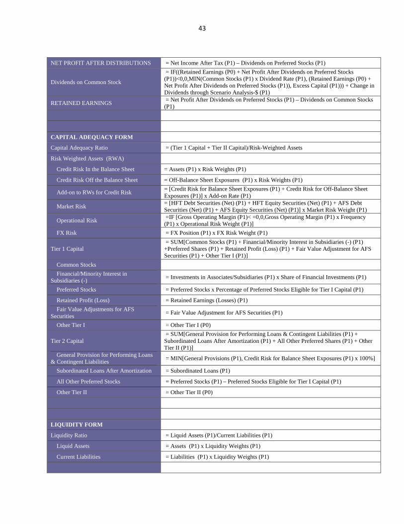
43

NET PROFIT AFTER DISTRIBUTIONS = Net Income After Tax (P1) – Dividends on Preferred Stocks (P1)

Dividends on Common Stock

= IF((Retained Earnings (P0) + Net Profit After Dividends on Preferred Stocks (P1))<0,0,MIN(Common Stocks (P1) x Dividend Rate (P1), (Retained Earnings (P0) + Net Profit After Dividends on Preferred Stocks (P1)), Excess Capital (P1))) + Change in Dividends through Scenario Analysis-$ (P1)

RETAINED EARNINGS = Net Profit After Dividends on Preferred Stocks (P1) – Dividends on Common Stocks (P1)

CAPITAL ADEQUACY FORM

Capital Adequacy Ratio = (Tier 1 Capital + Tier II Capital)/Risk-Weighted Assets

Risk Weighted Assets (RWA)

Credit Risk In the Balance Sheet = Assets (P1) x Risk Weights (P1)

Credit Risk Off the Balance Sheet = Off-Balance Sheet Exposures (P1) x Risk Weights (P1)

Add-on to RWs for Credit Risk = [Credit Risk for Balance Sheet Exposures (P1) + Credit Risk for Off-Balance Sheet Exposures (P1)] x Add-on Rate (P1)

Market Risk = [HFT Debt Securities (Net) (P1) + HFT Equity Securities (Net) (P1) + AFS Debt Securities (Net) (P1) + AFS Equity Securities (Net) (P1)] x Market Risk Weight (P1)

Operational Risk =IF [Gross Operating Margin (P1)< =0,0,Gross Operating Margin (P1) x Frequency (P1) x Operational Risk Weight (P1)]

FX Risk = FX Position (P1) x FX Risk Weight (P1)

Tier 1 Capital = SUM[Common Stocks (P1) + Financial/Minority Interest in Subsidiaries (-) (P1) +Preferred Shares (P1) + Retained Profit (Loss) (P1) + Fair Value Adjustment for AFS Securities (P1) + Other Tier I (P1)]

Common Stocks Financial/Minority Interest in

Subsidiaries (-) = Investments in Associates/Subsidiaries (P1) x Share of Financial Investments (P1)

Preferred Stocks = Preferred Stocks x Percentage of Preferred Stocks Eligible for Tier I Capital (P1)

Retained Profit (Loss) = Retained Earnings (Losses) (P1) Fair Value Adjustments for AFS

Securities = Fair Value Adjustment for AFS Securities (P1)

Other Tier I = Other Tier I (P0)

Tier 2 Capital = SUM[General Provision for Performing Loans & Contingent Liabilities (P1) + Subordinated Loans After Amortization (P1) + All Other Preferred Shares (P1) + Other Tier II (P1)]

General Provision for Performing Loans & Contingent Liabilities = MIN[General Provisions (P1), Credit Risk for Balance Sheet Exposures (P1) x 100%]

Subordinated Loans After Amortization = Subordinated Loans (P1)

All Other Preferred Stocks = Preferred Stocks (P1) – Preferred Stocks Eligible for Tier I Capital (P1)

Other Tier II = Other Tier II (P0)

LIQUIDITY FORM

Liquidity Ratio = Liquid Assets (P1)/Current Liabilities (P1)

Liquid Assets = Assets (P1) x Liquidity Weights (P1)

Current Liabilities = Liabilities (P1) x Liquidity Weights (P1)

44

FX POSITION FORM

FX Position Ratio = Net FX Position (P1)/Eligible Capital (P1)

Net FX Position-Local currency (LC.CY) = Eligible Capital (P1) x Net FX Position Rate (P1)

Eligible Capital = Eligible Capital (P1)

45

Appendix B. Methodology in Mathematical Notation

#BALANCE SHEET #1. ASSETS (1.1) HFT_Debt_Securities_Net(t+1) = HFT_Debt_Securities_Net(t) +

New_HFT_Debt_Securities_Net(t+1) – Reduction_of_HFT_Debt_Securities_to_Cover_Negative_Funds_Flow_Net_(t+1)

(1.2) Loans_Net(t+1) = Performing_Loans(t+1) + Non_Performing_Loans(t+1) - General_Provisions (-

)(t+1) - Specific_Provision (-)(t+1) (1.3) General_Provisions (-)(t+1) = Performing_Loans(t+1) * General_Provisioning_Rate(t+1) (1.4) Performing_Loans(t+1) = Performing_Loans(t) + New_Performing_Loans(t+1) +

Performing_Loans(t) * Default_Rate(t+1) + (Non_Performing_Loans(t) + Performing_Loans(t) * Default_Rate(t+1)) * Restructuring_Workout_Rate(t+1)

(1.5) Non_Performing_Loans(t+1) = Non_Performing_Loans(t) + Performing_Loans(t) *

Default_Rate(t+1) - (Non_Performing_Loans(t) + Performing_Loans(t) * Default_Rate(t+1)) * Restructuring_Workout_Rate(t+1) - (Non_Performing_Loans(t) + Performing_Loans(t) * Default_Rate(t+1)) * Foreclosure_Rate(t+1) (t+1) - (Non_Performing_Loans(t) + Performing_Loans(t) * Default_Rate(t+1)) * Write_off_Rate(t+1) - (Non_Performing_Loans(t) + Performing_Loans(t) * Default_Rate(t+1)) * Recovery_Rate(t+1)

(1.6) Specific_Provision (-)(t+1) = NonPerforming_Loans(t+1) * Specific_Provisioning_Rate(t+1) (1.7) Foreclosed_Assets(t+1) = Foreclosed_Assets(t) + (Non_Performing_Loans(t) + Performing_Loans(t)

* Default_Rate(t+1)) * Foreclosure_Rate(t+1) (1.8) Total_Assets(t+1) = HFT_Securities_Net(t+1) + Loans_Net(t+1) + Foreclosed_Assets_Net(t+1) #2. LIABILITIES & EQUITY #LIABILITIES (2.1) Deposits(t+1) = Deposits(t) * (1+ Growth_Rate_of_Deposits(t+1)) (2.2) Emergency_Lending _Assistance_(ELA)(t+1) = Final _Funds_Shortage_To_Be_Covered_by_ELA(t+1) (2.3) Total_Liabilities(t+1) = Deposits(t+1) + ELA(t+1) #SHAREHOLDER’S EQUITY (2.4) Paid_up_Capital(t+1) = Paid_up_Capital(t) (2.5) Retained_Earnings(t+1) = Retained_Earnings(t) + Net_Profit_After_Distributions(t+1)

46

(2.6) Total_Shareholder_Equity(t+1) = Paid_up_Capital(t+1) + Retained_Earnings(t+1) (2.7) Total_Liabilities_and_Equity(t+1) = Total_Shareholder_Equity(t+1) + Total Liabilities(t+1) # PROFIT AND LOSS ACCOUNT #3. INCOME STATEMENT (3.1) Total_Interest_Incomes(t+1) = HFT_Debt_Securities_Net(t+1) + Loans_Net(t+1) (3.2) HFT_Debt_Securities_Net(t+1) = HFT_Debt_Securities_Net(t) * Interest_Rate_on_Securities(t+1) (3.3) Loans_Net(t+1) = Performing_Loans(t) * Interest_Rate_on_Loans(t+1) (3.4) Total_interest_expenses(t+1) = Deposits(t+1) + ELA(t+1) (3.5) Deposits(t+1) = Deposits(t) * Interest_Rate_on_Deposits(t+1) (3.6) ELA(t+1) = ELA(t) * Interest_Rate_on_ELA(t+1) (3.7) Net_Interest_Incomes(t+1) = Total_Interest_Incomes(t+1) - Interest Expenses(t+1) (3.8) Operational_Expenses(-) (t+1) = (Performing_Loans(t+1) + Non_Performing_Loans(t+1)) * Operational_Expense_Rate(t+1) (3.9) Net_Operating_Incomes(t+1) = Net_Interest_Incomes(t+1) - Operational Expenses (-) (t+1) (3.10) Provisions (-)(t+1) = General_Provisions(t+1) - General_Provisions(t) + Specific_Provisions(t+1) – Specific_Provisions(t) + (Non_Performing_Loans(t) + Performing_Loans(t) * Default_Rate(t+1)) * Write_off_Rate(t+1) (3.11) Net_Income_Before_Distributions(t+1) = Net_Operating_Incomes(t+1) – Provisions (-)(t+1) (3.12) Dividends(t+1) = IF((Retained_Earnings(t) + Net_Income_Before_Distributions(t+1))<0,0,MIN(Paid_up_Capital(t+1) * Dividend_Rate(t+1), (Retained_Earnings(t) + Net_Income_After_Tax(t+1)))) (3.13) Net_Profit_After_Distributions(t+1) = Net_Income_Before_Distributions(t+1) - Dividends(t+1) # FUNDS FLOW STATEMENT #4. FUNDS FLOW (4.1) Funds_Flow(t+1) = Deposits(t+1) – Deposits(t) + Capital(t+1) – Capital(t) + Net_Profit_After_Distributions(t+1) + Provisions (-)(t+1) + (Non_Performing_Loans(t) + Performing_Loans(t) * Default_Rate(t+1)) * Recovery_Rate(t+1) (4.2) Payments_of_Previous_ELA(t+1) = ELA(t) (4.3) Funds_Flow_After_Paying_Previous_ELA (t+1) = Funds_Flow(t+1) – Payments_of_ELA(t+1)

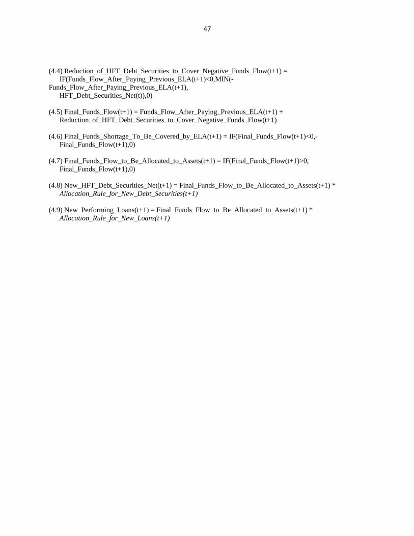
47

(4.4) Reduction_of_HFT_Debt_Securities_to_Cover_Negative_Funds_Flow(t+1) = IF(Funds_Flow_After_Paying_Previous_ELA(t+1)<0,MIN(-Funds_Flow_After_Paying_Previous_ELA(t+1), HFT_Debt_Securities_Net(t)),0) (4.5) Final_Funds_Flow(t+1) = Funds_Flow_After_Paying_Previous_ELA(t+1) + Reduction_of_HFT_Debt_Securities_to_Cover_Negative_Funds_Flow(t+1) (4.6) Final_Funds_Shortage_To_Be_Covered_by_ELA(t+1) = IF(Final_Funds_Flow(t+1)<0,- Final_Funds_Flow(t+1),0) (4.7) Final_Funds_Flow_to_Be_Allocated_to_Assets(t+1) = IF(Final_Funds_Flow(t+1)>0, Final_Funds_Flow(t+1),0) (4.8) New_HFT_Debt_Securities_Net(t+1) = Final_Funds_Flow_to_Be_Allocated_to_Assets(t+1) * Allocation_Rule_for_New_Debt_Securities(t+1) (4.9) New_Performing_Loans(t+1) = Final_Funds_Flow_to_Be_Allocated_to_Assets(t+1) * Allocation_Rule_for_New_Loans(t+1)

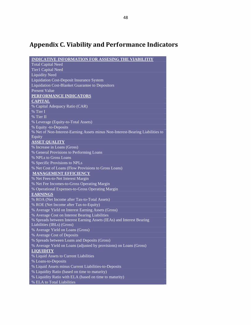
48

Appendix C. Viability and Performance Indicators INDICATIVE INFORMATION FOR ASSESING THE VIABILITIY Total Capital Need Tier1 Capital Need Liquidity Need Liquidation Cost-Deposit Insurance System Liquidation Cost-Blanket Guarantee to Depositors Present Value PERFORMANCE INDICATORS CAPITAL % Capital Adequacy Ratio (CAR) % Tier I % Tier II % Leverage (Equity-to-Total Assets) % Equity -to-Deposits % Net of Non-Interest-Earning Assets minus Non-Interest-Bearing Liabilities to Equity ASSET QUALITY % Increase in Loans (Gross) % General Provisions to Performing Loans % NPLs to Gross Loans % Specific Provisions to NPLs % Net Cost of Loans (Flow Provisions to Gross Loans) MANAGEMENT EFFICIENCY % Net Fees-to-Net Interest Margin % Net Fee Incomes-to-Gross Operating Margin % Operational Expenses-to-Gross Operating Margin EARNINGS % ROA (Net Income after Tax-to-Total Assets) % ROE (Net Income after Tax-to-Equity) % Average Yield on Interest Earning Assets (Gross) % Average Cost on Interest Bearing Liabilities % Spreads between Interest Earning Assets (IEAs) and Interest Bearing Liabilities (IBLs) (Gross) % Average Yield on Loans (Gross) % Average Cost of Deposits % Spreads between Loans and Deposits (Gross) % Average Yield on Loans (adjusted by provisions) on Loans (Gross) LIQUIDITY % Liquid Assets to Current Liabilities % Loans-to-Deposits % Liquid Assets minus Current Liabilities-to-Deposits % Liquidity Ratio (based on time to maturity) % Liquidity Ratio with ELA (based on time to maturity) % ELA to Total Liabilities

49

Appendix D. The World Bank Terms and Conditions

The International Bank for Reconstruction and Development and its officers, agents, employees, and content providers (referred to below as “The World Bank” or “we” or “us” or “our”) maintain this web site (the "Site") as part of efforts to provide broad public access to information. We encourage you to use the information and data it contains (the "Materials") as well as communications tools designed to facilitate this use. Unless explicitly stated otherwise, the Site, the Materials, those communications tools, and any new tools made available by us that alter or improve your use of the Site or the Materials shall be subject to this agreement (these “Terms and Conditions”), and by using the Site you consent to be bound hereby. The Financial Projection Model 2.0 (FPM 2.0) is also subject to this agreement.

For some of the Materials, such as the Datasets listed in The World Bank Data Catalog or the Publications made available in the Open Knowledge Repository, The World Bank has specific terms of use, all of which are hereby incorporated by reference. Those specific terms of use are available on the pages through which the relevant Materials are accessible, and are also collected here:

http://www.worldbank.org/terms-of-use-datasets

http://www.worldbank.org/terms-of-use-okr

For the remainder of the Materials, you may make non-commercial uses thereof, but you may not make any commercial use, including without limitation reselling them, charging to access them, charging to redistribute them, or charging for derivative works based on them. The foregoing license is conditioned upon your providing proper attribution to The World Bank and its content providers in the following format: “The World Bank: The World Bank authorizes the use of this material subject to the terms and conditions on its website, http://www.worldbank.org/terms.”

The World Bank administers this Site. The World Bank Group is comprised of IBRD (International Bank for Reconstruction and Development), IDA (International Development Association), IFC (International Finance Corporation), MIGA (Multilateral Guarantee Agency), and ICSID (International Centre for Settlement of Investment Disputes). All Materials on this Site from the various members of The World Bank Group, and other content providers, appear subject to these Terms and Conditions. In addition, the members of The World Bank Group and such content providers may have additional terms and conditions that govern the use of their material.

Unless expressly stated otherwise, the findings, interpretations, and conclusions expressed in the Materials in this Site are those of the various authors of the Materials and are not necessarily those of The World Bank Group's Boards of Executive Directors or its member countries.

No Endorsement

You may not publicly represent or imply that The World Bank is participating in, or has sponsored, approved, or endorsed the manner or purpose of your use or reproduction of the Materials. The World Bank will prosecute, to the fullest extent of the law, any use of World Bank Materials in a manner that falsifies, misrepresents, disparages, or fraudulently uses the Materials.

No Association

You may not use any trademark, official mark, official emblem, or logo of The World Bank, or any of its other means of promotion or publicity, without The World Bank's prior written consent nor in any event to represent or imply an association or affiliation with The World Bank.

Usernames and Interactive Tools

In order to access certain portions and features of the Site, you may have to create a “username” and complete an account registration process. If you do so, you agree to provide accurate, current, and complete information about yourself as prompted by the Site's registration forms. You also agree to update your account information in a prompt manner in order to keep it true, accurate, current and complete. You are responsible for maintaining the confidentiality of your account password and username, and are fully responsible for all activities that occur under your password or username. Please immediately notify The World Bank of any unauthorized use of your password or username or any other breach of security.

If this Site contains tools that enable you to “Post” (i.e., upload, post, make available, communicate, send, share, or transmit) Materials (collectively referred to as “Interactive Tools”), you agree not to use the Interactive Tools to do any of the following:

> Violate any applicable law or encourage or provide instructions to another to do so. > Defame, abuse, harass, stalk, threaten, or otherwise violate the legal rights (such as rights of privacy and publicity) of others. > Post any infringing, obscene, indecent, or unlawful material or information. > Misrepresent your identity. > Collect or store personal information about anyone. > Send “spam” email messages to anyone. > Upload or attach files that contain viruses, corrupted files, or any other similar software or programs that may damage the operation of another's computer. > Delete any author attributions, legal notices, or proprietary designations or labels in any file that is uploaded. > Falsify the origin or source of software or other material contained in a file that is uploaded. > Advertise or offer to sell any goods or services, or conduct or forward surveys, contests, or chain letters on the Site. > Download any file posted by another user that you know, or reasonably should know, cannot be legally distributed in such manner.

https://openknowledge.worldbank.org/

https://openknowledge.worldbank.org/

http://www.worldbank.org/terms-of-use-datasets

http://www.worldbank.org/terms-of-use-okr

http://www.worldbank.org/terms

50

You acknowledge that exchanges using Interactive Tools are public and not private communications. Further, you acknowledge that Postings by other users are not endorsed by The World Bank, and such Postings should not be considered reviewed, screened, or approved by The World Bank. The World Bank reserves the right for any or no reason to remove without notice any Materials or Posts received from users.

You grant The World Bank a royalty-free, irrevocable, transferrable, sublicensable, and non-exclusive perpetual license throughout the universe for use in any and all media whether now known or hereafter devised to use and exploit (including without limitation by reproduction, distribution, public display, adaptation, and/or public performance) any and all Materials that you Post.

Application Program Interfaces

The World Bank Application Programming Interfaces (“APIs”) are tools that allow you to retrieve and use certain Materials. The World Bank APIs enable retrieval of various Materials, grouped generally into calls to retrieve Materials found on the Site.

For use of the APIs in connection with some of the Materials (such as Datasets listed in The World Bank Data Catalog), The World Bank has specific terms of use, all of which are hereby incorporated by reference. Those specific terms of use are available on the pages through which the relevant Materials are accessible, and are also collected here: http://www.worldbank.org/terms-datasets. For use of the APIs in connection with other Materials, you may use the APIs to facilitate non-commercial uses of the Materials, but you may not use the APIs to facilitate commercial uses of the Materials, including without limitation reselling them, charging to access them, charging to redistribute them, or charging to create derivative works based on them.

The World Bank may release updated versions of the APIs at its sole discretion. New versions may not be compatible with previous implementations, and you agree to use the most recently updated version.

You agree not to modify, distribute, decompile, disassemble, or reverse engineer any portion of the APIs or any software of The World Bank.

You may not use the APIs in a manner that exceeds reasonable request volume or constitutes excessive or abusive usage, as determined by The World Bank at its sole discretion.

You may not use the APIs in a manner that is unlawful or that harms The World Bank, its service providers, its content providers, or any other person, as determined by The World Bank at its sole discretion.

The World Bank may monitor your use of the APIs. You may not use any technical means to interfere with such monitoring, and we may use technical means to overcome any such interference.

You agree not to facilitate access to Materials by using our APIs without entering into binding agreements with users of the Materials which limit use of the Materials in a manner that is consistent with these Terms and Conditions.

Please contact The World Bank at API [email protected] with any questions regarding the APIs.

Procedure for Sending Complaints Regarding Materials

If you believe that your rights, or the rights of a third party, including any intellectual property rights, are being violated in any way by any Materials on the Site, please contact us at:

Complaints: The World Bank Senior Vice President and Group General Counsel 1818 H Street, NW Washington, D C 20433 USA Tel: 202 473 3015 Fax: 202 522 1589 email: [email protected]

We will work to prevent unlawful activity from taking place on or through the Site.

Procedure for Sending Copyright Notices under the Digital Millennium Copyright Act

If you have a good faith belief that your copyright is being infringed by any Materials on the Site and you want to provide The World Bank with a notification of claimed infringement under the Digital Millennium Copyright Act (DMCA), please send a Notice of Claimed Infringement, including the information listed below, to The World Bank’s Designated Copyright Agent:

Designated Copyright Agent: The World Bank Senior Vice President and Group General Counsel 1818 H Street, NW Washington, D C 20433 USA Tel: 202 473 3015 Fax: 202 522 1589 email: [email protected]

The World Bank has instituted a policy designed to enable, at The World Bank’s sole discretion, the expeditious removal of infringing material and the termination of the usernames and access of users who qualify as repeat infringers. Please make sure that any Notice of Claimed Infringement you send to The World Bank’s Designated Copyright Agent includes all of the following:

> A physical or electronic signature of a person authorized to act on behalf of the owner of an exclusive right that is allegedly infringed. > An identification of the copyrighted work claimed to have been infringed, or, if multiple copyrighted works are covered by a single notification, a representative list of such works.

http://www.worldbank.org/terms-datasets

mailto:[email protected]



51

> An identification of the material that is claimed to be infringing or to be the subject of infringing activity and that is to be removed or access to which is to be disabled, and information reasonably sufficient to permit us to locate the material. > Information reasonably sufficient to permit us to contact you, such as an address, telephone number, and, if available, an electronic mail address at which you may be contacted. > A statement that you have a good faith belief that use of the material in the manner complained of is not authorized by the copyright owner, its agent, or the law. > A statement that the information in the notification is accurate, and, under penalty of perjury, that you are authorized to act on behalf of the owner of an exclusive right that is allegedly infringed.

Disclaimers, Releases, and Limitations on Liability

YOU USE THE SITE, MATERIALS AND API AT YOUR SOLE RISK. THE WORLD BANK PROVIDES THE SITE, MATERIALS, AND APIS "AS IS" AND "AS AVAILABLE". THE WORLD BANK EXPRESSLY DISCLAIMS TO THE FULL EXTENT PERMITTED BY LAW ALL WARRANTIES OF ANY KIND RELATED TO THE SITE, MATERIALS, AND APIS, WHETHER EXPRESS OR IMPLIED, INCLUDING, BUT NOT LIMITED TO, THE IMPLIED WARRANTIES OF MERCHANTABILITY, FITNESS FOR A PARTICULAR PURPOSE, AND NON-INFRINGEMENT. YOU WILL BE SOLELY RESPONSIBLE FOR ANY DAMAGE TO YOUR COMPUTER SYSTEM OR LOSS OF DATA THAT RESULTS FROM YOUR USE OF THE SITE, MATERIALS, OR APIS. THE WORLD BANK MAKES NO WARRANTY THAT (1) THE SITE, MATERIALS, OR APIS WILL MEET YOUR REQUIREMENTS; (2) THE SITE, MATERIALS OR APIS WILL BE UNINTERRUPTED, TIMELY, SECURE, OR ERROR-FREE; (3) THE RESULTS OF THE SITE, MATERIALS, OR APIS WILL BE ACCURATE OR RELIABLE; (4) THE QUALITY OF ANY PRODUCTS, SERVICES, OR MATERIAL OBTAINED BY YOU THROUGH THE SITE WILL MEET YOUR EXPECTATIONS; OR (5) THE SITE, ITS SERVERS, THE MATERIALS, OR APIS, OR COMMUNICATIONS SENT FROM THE WORLD BANK WILL BE FREE OF VIRUSES OR OTHER HARMFUL COMPONENTS. NO INFORMATION OBTAINED BY YOU FROM THE WORLD BANK OR THROUGH THE SITE SHALL CREATE ANY WARRANTY NOT EXPRESSLY STATED IN THESE TERMS AND CONDITIONS.

The World Bank may or may not review Materials that you Post, but it shall have the right (but not the obligation) in its sole discretion to review, reject, or remove any and all Materials at any time for any or no reason whatsoever with or without notice to you.

The World Bank reserves the right, at its sole discretion for any reason or no reason at any time and from time to time and with or without notice to you, to modify or discontinue, temporarily or permanently, the Site (or any part thereof) or to terminate your username and account and/or your access to the Site (or any part thereof). Under no circumstances shall The World Bank be liable for any loss, damage, liability, or expense incurred or suffered which is claimed to result from your use of this Site, including without limitation, any fault, error, omission, interruption, or delay with respect thereto.

Under no circumstances, including, but not limited to, negligence, shall The World Bank or ANY ENTITY THAT IS A MEMBER OF THE WORLD BANK GROUP, or any other content provider, be liable for any direct, indirect, incidental, special, EXEMPLARY, or consequential damages, even if The World Bank has been advised of the possibility of such damages.

You specifically acknowledge and agree that The World Bank is not liable for any conduct of any User. You hereby release The World Bank from claims, demands, and damages (actual and consequential) of every kind and nature, known and unknown, arising out of or in any way connected with the conduct of any User. You also waive California Civil Code §1542, which says: "A general release does not extend to claims which the creditor does not know or suspect to exist in his favor at the time of executing the release, which if known by him must have materially affected his settlement with the debtor." You also waive any and all benefits and rights that would otherwise accrue to you by reason of the provisions of any federal or state statute or principle of common law of any state of the United States, or any political entity or nation, province, or local law or regulation that may govern this release, which statute, regulation, law, or principle provides in substance something similar to California Civil Code § 1542.

This Site may contain advice, opinions, and statements of various content providers. The World Bank does not represent or endorse the accuracy or reliability of any advice, opinion, statement, or other information provided by any content provider, or any User of this site, or other person or entity. Reliance upon any such opinion, advice, statement, or other information shall also be at your own risk. The World Bank shall not be liable to any you or anyone else for any inaccuracy, error, omission, interruption, timeliness, completeness, deletion, defect, failure of performance, computer virus, communication line failure, alteration of, or use of any content herein, regardless of cause, for any damages resulting therefrom.

As a condition of use of this Site, you agree to indemnify The World Bank and other members of The World Bank Group from and against any and all actions, claims, losses, damages, liabilities, and expenses (including reasonable attorneys' fees) arising out of your use of this Site, including without limitation any claims alleging facts that if true would constitute a breach by you of these Terms and Conditions. You will cooperate as fully as reasonably required in the defense of any such claim. The World Bank reserves the right, at its own expense, to assume the exclusive defense and control of any matter otherwise subject to indemnification by you, and you shall not in any event settle any matter without the written consent of The World Bank.

Other parties may have ownership interests in some of the Materials contained on the Site. The World Bank in no way represents or warrants that it owns or controls all rights in all Materials, and The World Bank will not be liable to you for any claims brought against you by third parties in connection with your use of any Materials.

Nothing in this Site or any Materials shall be construed, implicitly or explicitly, as containing any investment recommendations. The World Bank is not registered under the U.S. Investment Advisers Act of 1940. Accordingly, nothing in such Site, or in such Materials, constitutes an offer of or an invitation by or on behalf of The World Bank to purchase or sell any shares or securities, nor should it be considered as investment advice.

This Site may contain links to third-party web sites. The linked sites are not under the control of The World Bank, which is not responsible for the contents of any linked site or any link contained in a linked site. The World Bank does not endorse the linked to sites.

52

You acknowledge that these Terms and Conditions constitute a non-exclusive agreement. The World Bank may develop products or services that compete with products or services that you offer without incurring any liability.

Governing Law

Any dispute between The World Bank and you arising out of, or in connection with, the Site or your use of the Site which cannot be amicably settled between the parties to such dispute shall be arbitrated in accordance with the Commercial Arbitration Rules of the American Arbitration Association then in effect by one arbitrator appointed in accordance with those rules. The arbitration shall take place in the District of Columbia. Any resulting arbitration decision shall be final and binding on both parties. Judgment upon any arbitration award in favor of The World Bank may be entered in any court having jurisdiction thereof. The World Bank Terms and Conditions and the relationship between you and The World Bank shall be governed by the laws of the District of Columbia as an agreement wholly performed therein without regard to its conflict of law provisions.

Preservation of Immunities

Nothing herein shall constitute or be considered to be a limitation upon or a waiver of the privileges and immunities of the International Bank for Reconstruction and Development or of any World Bank Group entity, which are specifically reserved.

Miscellaneous

These Terms and Conditions may be amended by The World Bank from time to time at our sole discretion. Upon amendment, we will place a notice on our homepage. Please periodically review the controlling version of these Terms and Conditions. By continuing to use the Site subsequent to The World Bank making available an amended version of these Terms and Conditions, you thereby acknowledge, agree, and consent to such amendment.

These Terms and Conditions include The World Bank Privacy Policy, available at http://www.worldbank.org/privacy, which is hereby incorporated by reference.

The failure of The World Bank to exercise or enforce any right or provision of these Terms and Conditions shall not constitute a waiver of such right or provision. No waiver by The World Bank of any provision of this Agreement shall be binding except as set forth in writing and signed by its duly authorized representative.

These Terms and Conditions are fully assignable by The World Bank and will be binding upon and inure to the benefit of our successors and assigns.

No agency, partnership, joint venture, employee-employer, or franchiser-franchisee relationship is intended or created by these Terms and Conditions. You agree not make any public statements that assert or imply any relationship with The World Bank, unless you have The World Bank's prior written approval.

If any provision of these Terms and Conditions is found by a court of competent jurisdiction to be invalid, the court should nevertheless endeavor to give effect to the parties' intentions as reflected in the provision, and the other provisions of these Terms and Conditions remain in full force and effect.

The World Bank reserves all rights not expressly granted under these Terms and Conditions, and no other rights are granted by implication or estoppel or otherwise.

The headings in these Terms and Conditions are for convenience only and have no legal or contractual effect.

http://www.worldbank.org/privacy

The Financial Projection Model 2.0 and its Implementation...

Documents

Transcript of The Financial Projection Model 2.0 and its Implementation...