Vortex Mathematics & The Fibonacci Spiral: Unlocking The Fibonacci Sequence

The Fibonacci Sequence Under Various Moduli
Marc Renault
May, 1996
A thesis submitted toWake Forest University
in partial fulfillment of the degree ofMaster of Arts in Mathematics

2

Contents
1 Leonardo of Pisa and the Fibonacci Sequence 3
2 The Binet Formula 11
3 Modular Representations of Fibonacci Sequences 173.1 The Period . . . . . . . . . . . . . . . . . . . . . . . . . . . . . . . . . . . . . 173.2 The Distribution Of Residues . . . . . . . . . . . . . . . . . . . . . . . . . . . 303.3 The Zeros Of F(mod m) . . . . . . . . . . . . . . . . . . . . . . . . . . . . . . 34
4 Personal Findings 474.1 Spirolaterals And The Fibonacci Sequence . . . . . . . . . . . . . . . . . . . . 474.2 Fibonacci Subsequences . . . . . . . . . . . . . . . . . . . . . . . . . . . . . . 55
A The First 30 Fibonacci and Lucas Numbers 63
B k(m), α(m), and β(m) for 2 ≤ m ≤ 1000 65
C One Period Of F (mod m) for 2 ≤ m ≤ 50 75
1

2 CONTENTS

Chapter 1
Leonardo of Pisa and theFibonacci Sequence
Fibonacci, the pen name of Leonardo of Pisa which means son of Bonacci, was born in Pisa,
Italy around 1170. Around 1192 his father, Guillielmo Bonacci, became director of the Pisan
trading colony in Bugia, Algeria, and some time thereafter they traveled together to Bugia.
From there Fibonacci traveled throughout Egypt, Syria, Greece, Sicily, and Provence where
he became familiar with Hindu-Arabic numerals which at that time had not been introduced
into Europe.
He returned to Pisa around 1200 and produced Liber Abaci in 1202. In it he presents
some of the arithmetic and algebra he encountered in his travels, and he introduces the place-
valued decimal system and Arabic numerals. Fibonacci continued to write mathematical
works at least through 1228, and he gained a reputation as a great mathematician. Not
much is known of his life after 1228, but it is commonly held that he died some time after
1240, presumably in Italy.
Despite his many contributions to mathematics, Fibonacci is today remembered for the
sequence which comes from a problem he poses in Liber Abaci. The following is a paraphrase:
A man puts one pair of rabbits in a certain place entirely surrounded by a wall.
The nature of these rabbits is such that every month each pair bears a new pair
which from the end of their second month on becomes productive. How many
pairs of rabbits will there be at the end of one year?
If we assume that the first pair is not productive until the end of the second month, then
3

4 CHAPTER 1. LEONARDO OF PISA AND THE FIBONACCI SEQUENCE
clearly for the first two months there will be only one pair. At the start of the third month
the first pair will beget a pair giving us a total of two pair. During the fourth month the
original pair begets again but the second pair does not, giving us three pair, and so on.
Assuming none of the rabbits die we can develop a recurrence relation. Let there be Fn
pairs of rabbits in month n, and Fn+1 pairs of rabbits in month n+1. During month n+2,
all the pairs of rabbits from month n + 1 will still be there, and of those rabbits the ones
which existed during the nth month will give birth. Hence Fn+2 = Fn+1 +Fn. The sequence
which ensues when F1 = F2 = 1 is called the Fibonacci sequence and the numbers in the
sequence are the Fibonacci numbers.
n: 1 2 3 4 5 6 7 8 9 10 11 12 ...Fn: 1 1 2 3 5 8 13 21 34 55 89 144 ...
Thus the answer to Fibonacci’s problem is 144.
Interestingly, it was not until 1634 that this recurrence relation was written down by
Albert Girard.
Despite its simple appearance the Fibonacci sequence contains a wealth of subtle and
fascinating properties. For example,
Theorem 1.1 Successive terms of the Fibonacci sequence are relatively prime.
Proof: Suppose that Fn and Fn+1 are both divisible by a positive integer d.
Then their difference Fn+1 − Fn = Fn−1 will also be divisible by d. Continuing,
we see that d|Fn−2, d|Fn−3, and so on. Eventually, we must have d|F1. Since
F1 = 1 clearly d = 1. Since the only positive integer which divides successive
terms of the Fibonacci sequence is 1, our theorem is proved.
One of the purposes of this chapter and the next is to develop many of the identities
needed in chapters three and four. All of these can be found in either [4] or [20]. Given
the recursive nature of the sequence, proof by induction is often a useful tool in proving
identities and theorems involving the Fibonacci numbers. One of the most useful is the
following.
Identity 1.2 Fm+n = Fm−1Fn + FmFn+1.

5
Proof: Let m be fixed and we will proceed by inducting on n. When n = 1,
then Fm+1 = Fm−1F1 + FmF2 = Fm−1 + Fm which is true.
Now let us assume the identity is true for n = 1, 2, 3, . . . , k, and we will show
that it holds for n = k + 1. By assumption
Fm+k = Fm−1Fk + FmFk+1
and
Fm+(k−1) = Fm−1Fk−1 + FmFk.
Adding the two we get Fm+k + Fm+(k−1) = Fm−1(Fk + Fk−1) + Fm(Fk+1 + Fk)
which implies Fm+(k+1) = Fm−1Fk+1 + FmFk+2 which is precisely our identity
when n = k + 1.
As an example of this identity, we see that F12 = F8+4 = F7F4 +F8F5 = 13(3)+21(5) =
144.
It is often useful to extend the Fibonacci sequence backward with negative subscripts.
The Fibonacci recurrence can be written as Fn = Fn+2 − Fn+1 which allows us to do this.
n: ... -7 -6 -5 -4 -3 -2 -1 0 1 2 3 4 ...Fn: ... 13 -8 5 -3 2 -1 1 0 1 1 2 3 ...
Sequences such as the Fibonacci sequence which can be extended infinitely in both directions
are called “bilateral”.
With some inspection another useful identity presents itself:
Identity 1.3 F−n = (−1)n+1Fn.
Now we can combine the above two identities to obtain
Identity 1.4 Fm−n = (−1)n(FmFn+1 − Fm+1Fn)
Another important fact about the Fibonacci sequence is easily tackled with induction.
Theorem 1.5 Fm|Fmn for all integers m,n.
Proof: Let m be fixed and we will induct on n. If either m or n equals zero,
then the theorem is true by easy inspection. For n = 1 it is clear that Fm|Fm.

6 CHAPTER 1. LEONARDO OF PISA AND THE FIBONACCI SEQUENCE
Now let us assume that the theorem holds for n = 1, 2, . . . , k and we will
show that it also holds for n = k + 1. Using identity 1.2 we see Fm(k+1) =
Fmk−1Fm + FmkFm+1. By assumption Fm|Fmk, and so Fm divides the entire
right side of the equation. Hence Fm divides Fm(k+1) and the theorem is proved
for n ≥ 1. Since Fmn differs from F−mn by at most a factor of -1, then Fm|Fmn
for n ≤ −1 as well.
A surprising result, with a surprisingly simple geometric proof is demonstrated in the
following identity.
Identity 1.6 F 21 + F 2
2 + F 23 + · · ·+ F 2
n = FnFn+1.
Proof: We can think of the squares of Fibonacci numbers as areas, and then
put them together in the manner below.
1 × 1 1 × 1
2× 2
3× 3
5× 5
8× 8. . .
...
We can find the area of the above rectangle by summing the squares, F 21 +F 2
2 +
F 23 +F 2
4 +F 25 +F 2
6 , or by multiplying height times width, F6 ·(F5 +F6) = F6 ·F7.
The general case for the sum of the squares of n Fibonacci numbers follows easily.
The following identity will be useful to us and it, too, can be proved geometrically.
Identity 1.7 F 2n + F 2
n+1 = F2n+1.

7
Proof:
Fn+Fn+1=Fn+2︷ ︸︸ ︷Fn × Fn
Fn+1 × Fn+1 Fn+1 − Fn = Fn−1
The area above can be represented as Fn−1Fn+1 + FnFn+2. From identity 1.2
this simplifies to Fn+(n+1) = F2n+1.
Here is another identity involving the square of Fibonacci numbers.
Identity 1.8 Fn+1Fn−1 − F 2n = (−1)n.
Proof:
Fn+1Fn−1 − F 2n = (Fn−1 + Fn)Fn−1 − F 2
n
= F 2n−1 + Fn(Fn−1 − Fn)
= F 2n−1 − FnFn−2
= −(FnFn−2 − F 2n−1).
We can now repeat the above process on the last line to attain
−(FnFn−2 − F 2n−1) = (−1)2(Fn−1Fn−3 − F 2
n−2)
= (−1)3(Fn−2Fn−4 − F 2n−3)
...
= (−1)n(F1F−1 − F 20 )
= (−1)n
It was the 19th century number theorist Edouard Lucas who first attached Fibonacci’s
name to the sequence we have been studying. He also investigated generalizations of the
sequence.
8 CHAPTER 1. LEONARDO OF PISA AND THE FIBONACCI SEQUENCE
A generalized Fibonacci sequence, G, is one in which the usual recurrence relation
Gn+2 = Gn+1+Gn holds, but G0 and G1 may take on arbitrary values. The Lucas sequence,
L, is an example of a generalized Fibonacci sequence where L0 = 2 and L1 = 1. It continues
2, 1, 3, 4, 7, 11, .... There are many interesting relationships between the Fibonacci and
Lucas sequences, and we give two of the most basic here.
Identity 1.9 Ln = Fn−1 + Fn+1.
Proof: We will prove the identity by induction. It is easy to see that L1 = 1 =
0 + 1 = F0 + F2 and L2 = 3 = 1 + 2 = F1 + F3. Now suppose that the identity
holds for Lr and Lr+1:
Lr = Fr−1 + Fr+1
Lr+1 = Fr + Fr+2
Adding the two equations gives us Lr+2 = Fr+1 + Fr+3 and subtracting the top
equation from the bottom yields Lr−1 = Fr−2 + Fr. Thus the identity holds for
all positive and negative r.
Identity 1.10 F2n = FnLn.
Proof: F2n = Fn+n = Fn−1Fn + FnFn+1 = Fn(Fn−1 + Fn+1) = FnLn.
We make a distinction between a Fibonacci sequence, meaning any generalized Fibonacci
sequence, and the Fibonacci sequence, meaning the sequence with G0 = 0 and G1 = 1.
Some authors generalize the sequence even more by using the relation Sn+2 = bSn+1 +
aSn. A further generalization examines sequences with the relation Sn = c1Sn−1 +c2Sn−2 +
· · · + ckSn−k for constants k and ci. Throughout this paper we will concentrate primarily
on the Fibonacci sequence, though we will have occasion to make use of the generalized
form Gn+2 = Gn+1 + Gn. We end this chapter with two identities from [20] involving the
generalized Fibonacci sequence.

9
Identity 1.11 Gm+n = Fn−1Gm + FnGm+1.
Proof: For the cases n = 0 and n = 1 we have
Gm = F−1Gm + F0Gm+1
Gm+1 = F0Gm + F1Gm+1
which is true since F−1 = 1, F0 = 0, and F1 = 1. By adding the two equations
it is easy to see that our identity continues to hold for n = 2, 3, . . . and so on.
Subtracting the first equation from the second indicates that the identity also
holds for negative n.
Identity 1.12 Gm−n = (−1)n(FnGm+1 − Fn+1Gm)
Proof: This identity follows by substituting −n for n in the above identity and
then using identity 1.3.

10 CHAPTER 1. LEONARDO OF PISA AND THE FIBONACCI SEQUENCE

Chapter 2
The Binet Formula
While the recurrence relation and initial values determine every term in the Fibonacci
sequence, it would be nice to know a formula for Fn so we wouldn’t have to compute all the
preceding Fibonacci numbers. Such a formula was discovered by Jacques-Philippe-Marie
Binet in 1843. Vajda [20] observes that this was actually a “rediscovery” since Abraham
DeMoivre knew about this formula as early as 1718. However, history has favored Binet
with the credit. Much of the material in this chapter can be found in [20].
Let us find the values for x which will give us the generalized Fibonacci sequence xn+2 =
xn+1 + xn. Since we are not concerned with the case where x = 0 which gives us the trivial
sequence, we may divide through by xn to attain x2 = x + 1, that is, x2 − x− 1 = 0. The
two roots of this equation are
τ =1 +
√5
2σ =
1−√
52
. (2.1)
Note the following properties of τ and σ:
τ + σ = 1 τ − σ =√
5 τσ = −1 (2.2)
Now 1, τ, τ2, τ3, . . . and 1, σ, σ2, σ3, . . . are in fact generalized Fibonacci sequences since
τn+2 = τn+1 + τn and σn+2 = σn+1 + σn. Indeed, any linear combination of τn and σn
forms the nth term of some Fibonacci sequence.
Gn = ατn + βσn (2.3)
As we see, (ατn+βσn)+(ατn+1+βσn+1) = α(τn+τn+1)+β(σn+σn+1) = ατn+2+βσn+2.
11

12 CHAPTER 2. THE BINET FORMULA
Any Fibonacci sequence can be expressed this way for particular values of α and β. We
show this by expressing α and β in terms of G0, G1, τ , and σ.
First, notice that G0 = α + β and G1 = ατ + βσ. Since β = G0 − α we can write
G1 = ατ + (G0 − α)σ
= α(τ − σ) + G0σ
= α√
5 + G0σ
which implies
α =G1 −G0σ√
5. (2.4)
Similarly α = G0 − β and so
G1 = (G0 − β)τ + βσ
= G0τ + β(σ − τ)
= G0τ − β√
5
which implies
β =G0τ −G1√
5. (2.5)
Now, once we know G0 and G1 we can use equations 2.4 and 2.5 to determine α and β, and
then the formula for Gn follows from equation 2.3.
For example, in the Fibonacci sequence F0 = 0 and F1 = 1, and so α = 1/√
5 and
β = −1/√
5. Thus
Fn =τn − σn
√5
. (2.6)
In the Lucas sequence L0 = 2 and L1 = 1.
α =1− 2σ√
5=
(τ + σ)− 2σ√5
=τ − σ√
5= 1.
β =2τ − 1√
5=
2τ − (τ + σ)√5
=τ − σ√
5= 1.
Thus
Ln = τn + σn. (2.7)
DeMoivre was able to derive the formula for Fn in a different way, using generating
functions. We demonstrate this technique next.
13
Let g(x) =∑∞
i=0 Fixi. It follows that g(x)− F0x
0 − F1x1 = g(x)− x. Hence
g(x)− x =∞∑
i=2
Fixi =
∞∑i=2
(Fi−1xi + Fi−2x
i)
= x∞∑
i=1
Fixi + x2
∞∑i=0
Fixi
= xg(x) + x2g(x).
Now we have g(x)− xg(x)− x2g(x) = x. That is,
g(x) =x
1− x− x2=
x
1− (τ + σ)x + τσx2
=x
(1− τx)(1− σx)=
(τ − σ)x√5(1− τx)(1− σx)
=1− σx√
5(1− τx)(1− σx)− 1− τx√
5(1− τx)(1− σx)
=1√
5(1− τx)− 1√
5(1− σx).
Expressing 11−τx and 1
1−σx as the sums of geometric series we get
g(x) =1√5(1 + τx + τ2x2 + · · ·)− 1√
5(1 + σx + σ2x2 + · · ·)
= [(τ − σ)x + (τ2 − σ2)x2 + · · ·]/√
5
The coefficient of xn, in other words Fn, is (τn − σn)/√
5, just as we suspected.
We can use the generating function to attain some unusual results. Taking our equation
g(x) =x
1− x− x2=
∞∑i=0
Fixi
and dividing through by x we get
11− x− x2
=∞∑
i=0
Fixi−1. (2.8)
When x = 1/2,
4 =∞∑
i=0
Fi
2i−1

14 CHAPTER 2. THE BINET FORMULA
which implies
2 =∞∑
i=0
Fi
2i. (2.9)
Another remarkable summation identity is obtained by differentiating both sides of equa-
tion (2.8)
1 + 2x
(1− x− x2)2=
∞∑i=0
(i− 1)Fixi−2.
When x = 1/2,
32 =∞∑
i=0
(i− 1)Fi
2i−2
8 =∞∑
i=0
(i− 1)Fi
2i=
∞∑i=0
iFi
2i−
∞∑i=0
Fi
2i
8 =∞∑
i=0
iFi
2i− 2
10 =∞∑
i=0
iFi
2i. (2.10)
The next identity is clearly more complicated than those we’ve looked at before, yet its
proof yields readily to the Binet formula. The interesting thing about it is that it gives us
insight into the recurrence relation governing subsequences of the Fibonacci sequence. This
identity shows how every nth term of the Fibonacci sequence is related.
15
Identity 2.1 Fm+n = LnFm + (−1)n+1Fm−n.
Proof:
LnFm + (−1)n+1Fm−n = (τn + σn)(τm − σm
√5
) + (−1)n+1(τm−n − σm−n
√5
)
=τm+n − τnσm + σnτm − σm+n
√5
+(−1)n+1τm−n − (−1)n+1σm−n
√5
=τm+n − (−1)nσm−n + (−1)nτm−n − σm+n − (−1)nτm−n + (−1)nσm−n
√5
=τm+n − σm+n
√5
= Fm+n
It is easy to see that when n = 1 in the above identity, we get the usual Fibonacci
recurrence relation, Fm+1 = (1)Fm + (1)Fm−1. When n = m we get identity 1.10: F2n =
LnFn.
Identity 2.2 Fn = 12n−1 [
(n1
)+
(n3
)5 +
(n5
)52 +
(n7
)53 + · · ·].
Proof:
Fn =τn − σn
√5
=1
2n√
5[(1 +
√5)n − (1−
√5)n]
Now expand using the binomial theorem:
=1
2n√
5
[(1 +
(n
1
)√5 +
(n
2
)√52
+(n
3
)√53
+ · · ·)
−(1−
(n
1
)√5 +
(n
2
)√52−
(n
3
)√53
+ · · ·)]
=1
2n−1√
5
[(n
1
)√5 +
(n
3
)√53
+(n
5
)√55
+ · · ·]
=1
2n−1
[(n
1
)+
(n
3
)5 +
(n
5
)52 +
(n
7
)53 + · · ·
]Lastly in this chapter we use τ and σ to demonstrate some simple greatest-integer iden-
tities. Though we will not use these, much research has been done in this area and they are
certainly of interest in their own right.

16 CHAPTER 2. THE BINET FORMULA
Identity 2.3 Fn = b τn√
5+ 1
2c for all n.
Proof: |Fn − τn√
5| = | σ
n√
5| < 1
2 for all n.
Identity 2.4 Fn+1 = bτFn + 12c for n ≥ 2.
Proof: |Fn+1 − τFn| = | τn+1−σn+1
√5
− τn+1−σnτ√5
| = |σn(τ−σ)√
5| = |σn| < 1
2 for all
n ≥ 2.

Chapter 3
Modular Representations ofFibonacci Sequences
One way to learn some fascinating properties of the Fibonacci sequence is to consider the
sequence of least nonnegative residues of the Fibonacci numbers under some modulus. One
of the first modern inquiries into this area of research was made by D. D. Wall [22] in 1960,
though J. L. Lagrange made some observations on these types of sequences in the eighteenth
century. Typically, the variable m will be used only to denote a modulus.
3.1 The Period
Perhaps the first thing one notices when the Fibonacci sequence is reduced mod m is that
it is periodic. For example,
F (mod 4) = 0 1 1 2 3 1 0 1 1 2 3 ...F (mod 5) = 0 1 1 2 3 0 3 3 1 4 0 4 4 3 2 0 2 2 4 1 0 1 1 2 3 ...
See appendix C for a list of the Fibonacci sequence under various moduli.
Any (generalized) Fibonacci sequence modulo m must repeat. After all, there are only
m2 possible pairs of residues and any pair will completely determine a sequence both forward
and backward. If we ignore the pair 0,0 which gives us the trivial sequence, then we know
that the period of any Fibonacci sequence mod m has a maximum length of m2 − 1.
It will always happen that the first pair to repeat will be the pair we started with.
Suppose that this were not so. Then we might have the sequence a, b, ..., x, y, ..., x, y, ...
where the pair a, b is not contained in the block x, y, ..., x, y. However, we know that this
17
18 CHAPTER 3. MODULAR REPRESENTATIONS OF FIBONACCI SEQUENCES
block repeats backward as well as forward, and so the pair a, b cannot be in the sequence.
This gives us our contradiction.
We can say some things about where the zeros will appear in the modular representation
of the Fibonacci sequence. Recall from identities 1.2 and 1.4 that
Fs+t = Fs−1Ft + FsFt+1
Fs−t = (−1)t(FsFt+1 − Fs+1Ft).
If Fs ≡ Ft ≡ 0 then clearly Fs+t ≡ 0 and Fs−t ≡ 0. Hence all the zeros of F (mod m) are
evenly spaced throughout the sequence. Since F (mod m) is periodic for any m and F0 = 0
we can say that any integer will divide infinitely many Fibonacci numbers. In addition,
all the Fibonacci numbers divisible by a given integer are evenly spaced throughout the
sequence.
We know that F (mod m) is periodic, so the question naturally presents itself: What is
the relationship between the modulus of a sequence and its period? We will examine some
results in this area.
Each author seems to have his or her own notation, but the following definitions come
from Wall. Let k(m) denote the period of the Fibonacci sequence modulo m. Let h(m)
denote the period of any generalized Fibonacci sequence modulo m. From our previous ex-
ample we see that k(4) = 6 and k(5) = 20. The following are some immediate consequences
of the definition.
Fn ≡ Fn+r·k(m) (mod m)
Gn ≡ Gn+r·h(m) (mod m)
Fk(m) ≡ 0 (mod m) (3.1)
Fk(m)−1 ≡ Fk(m)+1 ≡ Fk(m)+2 ≡ 1 (mod m) (3.2)
We will often use the fact that if Fn ≡ 0 (mod m) and Fn+1 ≡ 1 (mod m) then k(m)|n.
This result follows immediately from the periodicity of F (mod m).
We now demonstrate some very general properties of F (mod m) using our notation.
The following three theorems can be found in [22]. The reader is encouraged to examine the
table in appendix B which gives the period of F (mod m) for 2 ≤ m ≤ 1000, and observe the

3.1. THE PERIOD 19
behavior of k(m) as m varies. After noticing that F (mod m) is periodic one notices that
almost all of the periods are even. Though Wall provides the next theorem, the proof is the
author’s.
Theorem 3.1 For m ≥ 3, k(m) is even.
Proof: For ease of notation let k = k(m), and we will consider all congruences
to be taken modulo m. From identity 1.3 we know that if t is odd then Ft = F−t
and if t is even then Ft = −F−t. We will assume k to be odd and show that m
must equal 2.
We know that F1 = F−1 ≡ Fk−1. Now k−1 is even so Fk−1 = −F1−k ≡ −F1.
Thus F1 ≡ −F1, and as a result m = 2.
Another curious feature of F (mod m) is that k(n)|k(m) whenever n|m. Surprisingly,
this property is true of generalized Fibonacci sequences as well.
Theorem 3.2 If n|m, then for a given Fibonacci sequence, h(n)|h(m).
Proof: Let h = h(m). We need to show that G(mod n) repeats in blocks
of length h. We do this by showing that Gi ≡ Gi+h (mod n) regardless of our
choice for i. Certainly we know that Gi ≡ Gi+h (mod m), so for some 0 ≤ a < m
we have Gi = a + mx and Gi+h = a + my.
Now say m = nr and let us substitute nr for m in the previous two equations.
Then Gi = a+nrx and Gi+h = a+nry. We can say that a = a′+nw (0 ≤ a′ < n)
and this time substitute for a in the previous equations. Now Gi = a′+n(w+rx)
and Gi+h = a′+n(w+ry). Of course this implies that Gi ≡ Gi+h (mod n) which
was needed to be shown.
We can make this theorem more exact by expressing h(m) in terms of h(peii ) where m
has the prime factorization m =∏
peii .
Theorem 3.3 Let m have the prime factorization m =∏
peii . Then h(m) = lcm[h(pei
i )],
the least common multiple of the h(peii ).

20 CHAPTER 3. MODULAR REPRESENTATIONS OF FIBONACCI SEQUENCES
Proof: By our previous theorem h(peii )|h(m) for all i. It follows that lcm[h(pei
i )]|h(m).
Second, since h(peii )|lcm[h(pei
i )] we know G(mod peii ) repeats in blocks of
length lcm[h(peii )]. Hence Glcm[h(p
eii
)] ≡ G0 and Glcm[h(peii
)]+1 ≡ G1 (mod peii )
for all i. Since all the peii are relatively prime, the Chinese Remainder Theo-
rem assures us that Glcm[h(peii
)] ≡ G0 and Glcm[h(peii
)]+1 ≡ G1 (mod m). Thus
G(mod m) repeats in blocks of length lcm[h(peii )] and we can say that h(m)|lcm[h(pei
i )].
This concludes the proof.
Hence we have reduced the problem of characterizing k(m) into the problem of charac-
terizing k(pe). Before we develop theorems which speak to this problem, however, we look
at a related result. We see in the following theorem that it is not necessary to break a
modulus all the way into its prime factorization in order to attain information about k(m).
Theorem 3.4 h([m,n]) = [h(m), h(n)] where brackets denote the least common multiple
function.
Proof: Since m|[m,n] and n|[m,n] we know that h(m)|h([m,n]) and h(n)|h([m,n]).
It follows that [h(m), h(n)]|h([m,n]).
Say we have the prime factorization [m,n] = pe11 . . . pet
t . Then h([m,n]) =
h(pe11 . . . pet
t ) = [h(pe11 ) . . . h(pet
t )]. Since peii divides m or n for all i, certainly
h(peii ) divides h(m) or h(n) for all i. Thus [h(pe1
1 ) . . . h(pett )]|[h(m), h(n)]. In
other words, h([m,n])|[h(m), h(n)].
Hence h([m,n]) = [h(m), h(n)].
Now we turn our attention back to the matter of solving k(pe) in terms of pe. The general
case of this theorem is somewhat involved, so to motivate the ideas we look at a couple of
specific cases. We will demonstrate that k(2e) = 3 ·2e−1 and k(5e) = 4 ·5e. These results can
be found in [11], but the proofs there are somewhat incomplete. For example, Kramer and
Hoggatt show that F3·2e−1 ≡ 0 (mod 2e) and F3·2e−1+1 ≡ 1 (mod 2e) and they immediately
conclude that k(2e) = 3 · 2e−1. However, this only demonstrates that k(2e)|3 · 2e−1. The
proof below takes this point into consideration.
Theorem 3.5 k(2e) = 3 · 2e−1.

3.1. THE PERIOD 21
Proof: By inspection, k(2) = 3 and k(4) = 6, so the theorem holds for e = 1, 2.
Suppose k(2r) = 3 · 2r−1, so that F3·2r−1 ≡ 0 and F3·2r−1+1 ≡ 1 (mod 2r) and
we will induct on r.
By identity 1.10,
F3·2r = (F3·2r−1)(F3·2r−1−1 + F3·2r−1+1)
The first factor on the right, F3·2r−1 ≡ 0 (mod 2r). It is an easy matter to see
that every third Fibonacci number is even and the rest are odd, so the second
factor on the right, F3·2r−1−1 + F3·2r−1+1 ≡ 0 (mod 2). Thus their product,
F3·2r ≡ 0 (mod 2r+1).
By identity 1.7,
F3·2r+1 = (F3·2r−1)2 + (F3·2r−1+1)2
≡ (0 or 2r)2 + (1 or 2r + 1)2 (mod 2r+1)≡ 0 + 1 (mod 2r+1)≡ 1 (mod 2r+1)
Thus we know k(2r+1)|3 · 2r.
We know that k(2r)|k(2r+1), and by our induction hypothesis k(2r) = 3 ·
2r−1. Thus k(2r+1) = either 3 · 2r−1 or 3 · 2r. We will show that the latter is
true by proving F3·2r−1+1 6≡ 1 (mod 2r+1). More precisely, we will prove that
F3·2r−1+1 ≡ 2r + 1 (mod 2r+1).
Let us add this statement to our induction hypothesis: assume F3·2r−2 ≡ 0
and F3·2r−2+1 ≡ 2r−1 + 1 (mod 2r). By inspection this is the case for r = 3. We
will induct on r to show that F3·2r−1+1 ≡ 2r + 1 (mod 2r+1).
By identity 1.7,
F3·2r−1+1 = (F3·2r−2+1)2 + (F3·2r−2)2.
Let us look at the first term on the right.
F3·2r−2+1 ≡ (2r−1 + 1) or (2r−1 + 1 + 2r) (mod 2r+1)
(2r−1 + 1)2 = 22r−2 + 2r + 1 ≡ 2r + 1 (mod 2r+1)
(2r−1 + 1 + 2r)2 = (3 · 2r−1 + 1)2
= 9 · 22r−2 + 3 · 2r + 1 ≡ 2r + 1 (mod 2r+1)
22 CHAPTER 3. MODULAR REPRESENTATIONS OF FIBONACCI SEQUENCES
Thus
(F3·2r−2+1)2 ≡ 2r + 1 (mod 2r+1).
Let us look at the second term on the right.
F3·2r−2 ≡ 0 or 2r (mod 2r+1)
02 ≡ 0 (mod 2r+1)
(2r)2 = 22r ≡ 0 (mod 2r+1)
Thus
(F3·2r−2)2 ≡ 0 (mod 2r+1).
Consequently F3·2r−1+1 ≡ 2r + 1 (mod 2r+1) and the theorem follows.
Before we prove a similar theorem for k(5e) we first need to mention a lemma which
provides insight into one of the divisibility properties of the Fibonacci sequence.
Lemma 3.6 Let p be an odd prime and suppose pt|Fn but pt+16 |Fn for some t ≥ 1. If p6 | v
then pt+1|Fnvp but pt+26 | Fnvp.
The proof of this lemma is too involved to be examined here, but it can be found in [20].
Since F5 = 5, clearly 5 goes into F5 once. By the the lemma then, 5 goes into Fn·5t
exactly t times if 56 | n.
Theorem 3.7 k(5e) = 4 · 5e.
Proof: First we will show that for all e, F4·5e ≡ 0 and F4·5e+1 ≡ 1 (mod 5e).
By the lemma above clearly F4·5e ≡ 0 (mod 5e). From identity 1.7 we have
F4·5e+1 = (F2·5e)2 + (F2·5e+1)2.
Applying our lemma to the first term on the right gives us (F2·5e)2 ≡ 02 ≡
0 (mod 5e). By identity 1.8, the second term on the right, (F2·5e+1)2 = F2·5eF2·5e+2+
(−1)2·5e+2 ≡ 1 (mod 5e).
Thus we know that F4·5e ≡ 0 and F4·5e+1 ≡ 1 (mod 5e) and it follows that
k(5e)|4 · 5e for all e.

3.1. THE PERIOD 23
We proceed now by induction using the hypothesis k(5r) = 4 · 5r. By inspec-
tion this is the case for r = 1. We induct on r to show k(5r+1) = 4 · 5r+1.
Since 4 · 5r = k(5r)|k(5r+1) and k(5r+1)|4 · 5r+1, we know k(5r+1) = either
4 · 5r or 4 · 5r+1. In the first case, F4·5r contains exactly r factors of 5 and hence
F4·5r 6≡ 0 (mod 5r+1). Hence we must have k(5r+1) = 4 · 5r+1 and our theorem
is proved.
We have proved k(pe) = pe−1k(p) for p = 2 and p = 5, and we now turn to proving it
for all p. While the general theorem is slightly less strict than these special cases, it does
give us great insight into the periodic behavior of the Fibonacci sequence. One proof, by
Robinson[15], also shows how matrices may be used to discover facts about the Fibonacci
sequence. We will be working with the matrix U defined by
U =[
0 11 1
]which has the property that
Un =[
Fn−1 Fn
Fn Fn+1
]. (3.3)
This matrix has been called the Fibonacci matrix because of this property. Note that
Uk(m) = I + mB ≡ I (mod m) for some 2 × 2 matrix B. And, if Un ≡ I (mod m) then
k(m)|n.
Theorem 3.8 If t is the largest integer such that k(pt) = k(p) then k(pe) = pe−tk(p) for
all e ≥ t.
Proof: Since Uk(pe) = I + peB we can write Upk(pe) = (I + peB)p = Ip +(p1
)Ip−1(peB) +
(p2
)Ip−2(peB)2 + · · ·. Thus Upk(pe) ≡ I (mod pe+1). Clearly
Uk(pe+1) ≡ I (mod pe+1) and so we have k(pe+1)|pk(pe). Combine this fact with
the knowledge that k(pe)|k(pe+1) and as a result k(pe+1) = k(pe) or pk(pe).
Now let us assume that k(pe+1) = pk(pe) and we will induct on e to arrive
at k(pe+2) = pk(pe+1).
By assumption k(pe) 6= k(pe+1) and so we know that Uk(pe) = I +peB where
p6 |B. Hence Upk(pe) = (I +peB)p = Ip +(
p1
)Ip−1(peB)+
(p2
)Ip−2(peB)2 + · · · ≡
I +pe+1B (mod pe+2). (The astute reader may notice that this congruence does
24 CHAPTER 3. MODULAR REPRESENTATIONS OF FIBONACCI SEQUENCES
not actually hold for p = 2, e = 1. However, since we have proven the case for
p = 2 in theorem 3.5 we may assume p ≥ 3.) That is, Uk(pe+1) = Upk(pe) ≡
I + pe+1B 6≡ I (mod pe+2). This implies k(pe+1) 6= k(pe+2) so we must have
k(pe+2) = pk(pe+1) and the induction is complete.
Now let t be the largest e such that k(pe) = k(p). Then k(pe) = k(p) for
1 ≤ e ≤ t and k(pe) = k(pe−t) for e ≥ t.
Remarkably, the conjecture that t = 1 for all primes has existed since Wall’s paper
in 1960, but neither a proof nor a counter example has yet been found. Once again we
have been able to reduce the problem of finding the period of the Fibonacci sequence given
a modulus. All that remains (other than proving t = 1 for all primes, of course) is to
characterize k(p) in terms of p. However, this undertaking has proven to be extraordinarily
difficult, and the best we can do is to describe some bounds on k(p).
Theorems 3.11 through 3.13 will describe upper bounds on k(p), but we must first take
some time to develop certain divisibility properties of the Fibonacci sequence found in [20].
We will make use of these three facts for primes, p:
(i)( p
n
)≡ 0 (mod p) for 1 ≤ n ≤ p− 1
(ii)(
p− 1n
)≡ (−1)n (mod p) for 0 ≤ n ≤ p− 1
(iii)(
p + 1n
)≡ 0 (mod p) for 2 ≤ n ≤ p− 1
We will also use the following lemma:
Lemma 3.9 5 is a quadratic residue modulo primes of the form 5t ± 1 and a quadratic
nonresidue modulo primes of the form 5t± 2.
Proof: Using the Legendre symbol and the law of quadratic reciprocity we
know that ( 5p ) = (p
5 ) since 5 is a prime of the form 4t + 1. Then,(5
5t + 1
)=
(5t + 1
5
)=
(15
)= 1
(5
5t− 1
)=
(5t− 1
5
)=
(45
)= 1.
3.1. THE PERIOD 25
However, (5
5t + 2
)=
(5t + 2
5
)=
(25
)= −1
(5
5t− 2
)=
(5t− 2
5
)=
(35
)= −1.
Using identity 2.2 we have 2p−1Fp =(
p1
)+
(p3
)5 + · · ·+
(pp
)5
p−12 . Applying (i) above
and Fermat’s theorem we get Fp ≡ 5p−12 (mod p). Now from the lemma we know that
5p−12 ≡ 1 (mod p) if and only if p = 5t±1, and 5
p−12 ≡ −1 (mod p) if and only if p = 5t±2.
Hence,
If a prime p is of the form 5t± 1 then Fp ≡ 1 (mod p).If a prime p is of the form 5t± 2 then Fp ≡ −1 (mod p).
The converse of these statements is not true, for in fact F22 = 17711 = 85(22) + 1 ≡
1 (mod 22), and quite clearly, 22 is not prime.
Again we use identity 2.2 and see 2p−2Fp−1 =(
p−11
)+
(p−13
)5 + · · ·+
(p−1p−2
)5
p−32 . By
(ii) above, 2p−2Fp−1 ≡ −(1 + 5 + 52 + · · ·+ 5p−32 ) (mod p). Summing the geometric series
yields,
2p−2Fp−1 ≡ −5p−12 − 14
(mod p).
Clearly if 5p−12 ≡ 1 (mod p) then 2p−2Fp−1 ≡ 0 (mod p). Certainly 2p−2 6≡ 0 (mod p) so it
would have to be that Fp−1 ≡ 0 (mod p). Hence,
If a prime p is of the form 5t± 1 then Fp−1 ≡ 0 (mod p).
Finally, identity 2.2 gives us 2pFp+1 =(
p+11
)+
(p+13
)5 + · · · +
(p+1
p
)5
p−12 . By (iii)
above, 2pFp+1 ≡(
p+11
)+
(p+1
p
)5
p−12 = (p + 1) + (p + 1)5
p−12 ≡ 1 + 5
p−12 (mod p). Now
when 5p−12 ≡ −1 (mod p) we will have 2pFp+1 ≡ 0 (mod p). Since 2p ≡ 2 (mod p), it would
have to be that Fp+1 ≡ 0 (mod p). Thus,
If a prime p is of the form 5t± 2 then Fp+1 ≡ 0 (mod p).
Collecting our results provides us with the following theorem.
Theorem 3.10 If a prime p is of the form 5t± 1 then Fp−1 ≡ 0 and Fp ≡ 1 (mod p). If a
prime p is of the form 5t± 2 then Fp ≡ −1 and Fp+1 ≡ 0 (mod p).
26 CHAPTER 3. MODULAR REPRESENTATIONS OF FIBONACCI SEQUENCES
Now at last we can present some theorems concerning the character of k(p).
Theorem 3.11 If p is a prime, p 6= 5, then k(p)|p2 − 1.
Proof: By inspection, k(2) = 3, and the theorem holds for p = 2. Now let
us assume p odd. To prove the theorem we will show that Fp2−1 ≡ 0 and
Fp2 ≡ 1 (mod p).
If p = 5t ± 1 then p|Fp−1. We know that p − 1|p2 − 1 and so Fp−1|Fp2−1.
Hence p|Fp2−1. If p = 5t ± 2 then p|Fp+1. We know that p + 1|p2 − 1 and so
Fp+1|Fp2−1. Hence p|Fp2−1. Thus for all p 6= 5, Fp2−1 ≡ 0 (mod p).
To prove Fp2 ≡ 1 (mod p), we first note that 2p2−1Fp2 =(
p2
1
)+
(p2
3
)5 +
· · · +(
p2
p2
)5
p2−12 . Now 2p2−1 = (2p−1)p+1 ≡ 1 (mod p) and
(p2
n
)≡ 0 (mod p)
for 1 ≤ n ≤ p2 − 1. Hence Fp2 ≡ (5p−12 )p+1 ≡ (±1)p+1 ≡ 1 (mod p).
Thus the theorem is proved.
Theorem 3.12 If a prime p is of the form 5t± 1 then k(p)|p− 1.
Proof: Since p = 5t ± 1, theorem 3.10 tells us that Fp−1 ≡ 0 and Fp ≡
1 (mod p). Hence F (mod p) repeats in blocks of length p− 1. Thus k(p)|p− 1.

3.1. THE PERIOD 27
Theorem 3.13 If a prime p is of the form 5t± 2 then k(p)|2p + 2.
Proof: Suppose p = 5t ± 2. By theorem 3.10 then, Fp+1 ≡ 0 (mod p). Since
p + 1|2p + 2 and the zeros of F (mod p) are evenly spaced, we can say F2p+2 ≡
0 (mod p).
We also know that Fp ≡ −1 (mod p). By the usual recurrence relation
then, Fp+2 ≡ Fp+3 ≡ −1 (mod p). Now we can write F2p+3 = F(p+1)+(p+2) =
FpFp+2 + Fp+1Fp+3 ≡ (−1)(−1) + (0)(−1) ≡ 1 (mod p).
Thus k(p)|2p + 2.
We now consider upper and lower bounds for k(m) where m can be any integer m ≥ 2.
It was noted earlier that k(m) ≤ m2 − 1, but can we do better than this? One method of
determining an upper bound is to use the two preceding theorems to show that k(p) = p2−1
if and only if p = 2 or 3. Then by application of theorem 3.8 it can be proved that k(pe) <
(pe)2 − 1 for e ≥ 2. Finally, we can use theorem 3.4 to demonstrate that k(m) < m2 − 1 for
all composite m.
However, the author would like to propose a more elegant way of proving this inequality.
If k(m) = m2 − 1 for some m, then every possible pair of residues except 0, 0 appears in
F (mod m). It will be seen in section 3.3 that a single period of F (mod m) contains at most
four zeros. Consequently, F (mod m) contains at most four 0, r pairs where 1 ≤ r < m.
Hence, for m ≥ 6 there is some 0, r pair not represented in F (mod m) and we must have
k(m) < m2 − 1. It is a simple matter to check the remaining cases. When m = 2 or 3,
k(m) = m2 − 1 and when m = 4 or 5, k(m) < m2 − 1.
Unfortunately, empirical evidence indicates that this upper bound becomes less and less
precise as m increases. For 2 ≤ m ≤ 299 we find by inspection that k(m) ≤ 6m. For
300 ≤ m ≤ 1000 we find k(m) ≤ 4m. There does not appear to be any other material
published concerning upper bounds on k(m).
A sharp lower bound on k(m) was given by Paul Catlin[5] in 1974. We see here an
interesting interaction between the Lucas and Fibonacci numbers. We present his theorem
without proof.
28 CHAPTER 3. MODULAR REPRESENTATIONS OF FIBONACCI SEQUENCES
Theorem 3.14 Given a modulus m > 2, let t be any natural number such that Lt ≤ m.
Then k(m) ≥ 2t with equality if and only if Lt = m and t is odd.
In the beginning of the section we saw some results which helped to define the overall
character of h(m) and thus of k(m). In the last part of this section we present some results
due to Wall on the relationship between h(m) and k(m). The first of these is strikingly
simple.
Theorem 3.15 h(m)|k(m).
Proof: For ease of notation, let k = k(m). Applying identity 1.11 and then
equations 3.1 and 3.2 we get Gk = Fk−1G0 + FkG1 ≡ G0 (mod m) and Gk+1 =
FkG0 + Fk+1G1 ≡ G1 (mod m). Thus G(mod m) repeats in blocks of length
k(m). From this we can conclude h(m)|k(m).
We can elicit equality between h(m) and k(m) by putting stricter conditions on m.
Theorem 3.16 If a prime p is of the form 5t± 2 then h(pe) = k(pe).
Proof: For ease of notation, let h = h(pe). Certainly,
Gh −G0 ≡ 0 (mod pe), and
Gh−1 −G1 ≡ 0 (mod pe).
By identity 1.11 the above is equivalent to
(Fh−1G0 + FhG1)−G0 = G1Fh + G0(Fh−1 − 1) ≡ 0 (mod p)
(Fh−1G1 + Fh+1G2)−G1 = G2Fh + G1(Fh−1 − 1) ≡ 0 (mod p)
We now have a system of equations which we may treat as a matrix with
determinant D = G21 − G0G2. We will assume that D ≡ 0 (mod p) and arrive
at a contradiction.
When D ≡ 0 (mod p) then G21−G0G2 = G2
1−G0(G0 + G1) = G21−G0G1−
G20 ≡ 0 (mod p). This last congruence is impossible if p = 2 (we ignore the

3.1. THE PERIOD 29
trivial case G0 = G1 = 0) so we may assume p to be odd. Multiply both sides
by −4.
4G20 + 4G0G1 − 4G2
1 ≡ 0 (mod p)
Add 5G21 to both sides.
4G20 + 4G0G1 + G2
1 = (2G0 + G1)2 ≡ 5G21 (mod p)
Now multiply both sides by Gp−31 and apply Fermat’s theorem to the right.
Gp−31 (2G0 + G1)2 ≡ 5 (mod p)
Since p is odd, this implies that 5 is a quadratic residue modulo p. However,
by lemma 3.9, this contradicts our hypothesis that p = 5t ± 2. Therefore,
D 6≡ 0 (mod p), and this implies that D 6≡ 0 (mod pe).
Since the determinant of our matrix is not congruent to zero (mod pe), it
must have a unique solution modulo pe. Certainly Fh ≡ 0 and (Fh−1 − 1) ≡
0 (mod pe) satisfy the system, and so Fh ≡ 0 and Fh−1 ≡ 1 (mod pe). From the
recurrence relation, Fh+1 ≡ 1 (mod pe) as well.
Since h = h(pe) our results tell us that k(pe)|h(pe). By theorem 3.15 we
know h(pe)|k(pe). Hence h(pe) = k(pe).
Wall proved several other results regarding the relationship between h(m) and k(m). We
present some of these here without proof. As usual, p denotes a prime number.
Theorem 3.17 Let D = G21 −G0G1 −G2
0. If gcd(D,m) = 1 then h(m) = k(m).
Theorem 3.18 If h(pe) = 2t + 1 for some generalized Fibonacci sequence, then k(pe) =
4t + 2.
Theorem 3.19 If p > 2 and k(pe) = 4t + 2 then there exists some generalized Fibonacci
sequence where h(pe) = 2t + 1.
Theorem 3.20 Let p be odd and p 6= 5. If h(pe) is even then h(pe) = k(pe).
We end the section with two curious theorems pertaining to the period of F (mod m)
which did not seem to fit logically elsewhere within this section. We defer their proofs to the
30 CHAPTER 3. MODULAR REPRESENTATIONS OF FIBONACCI SEQUENCES
end of section 3.3 where we will have developed other ideas sufficiently to make their proofs
easy. The curious feature here is that the modulus of the sequence is an actual Fibonacci
or Lucas number. Theorem 3.45 can be found in [7] and theorem 3.46 can be found in [17].
Theorem 3.45 If n ≥ 5 is odd then k(Fn) = 4n. If n ≥ 4 is even then k(Fn) = 2n.
Theorem 3.46 If n ≥ 3 is odd then k(Ln) = 2n. If n ≥ 2 is even then k(Ln) = 4n.
These theorems indicate that for any even t ≥ 6 there is some m such that k(m) = t.
Also, k(m) can not equal 4, otherwise F4 = 3 ≡ 0 and F3 = 2 ≡ 1 (mod m) which is not
possible. Hence the range of k(m) is 3 union the set of all even numbers greater than or
equal to 6.
3.2 The Distribution Of Residues
In this section we look at what is known about the distribution of residues within a single
period of F (mod m). That is, how frequently each residue is expected to appear. We start
off with a more specific question: for which moduli will all the residues appear with equal
frequency within a single period? If F (mod m) exhibits this property it is said to be uniform
or uniformly distributed. Kuipers and Shiue[12] proved that the only time F (mod m) can
possibly be uniform is when m = 5e.
It is not difficult to see that if F (mod m) is uniform, then necessarily m|k(m). We use
this requirement to prove that 5 is the only prime for which F (mod p) is uniform.
We first note that by inspection F (mod 2) is not uniform but F (mod 5) is, with each
residue appearing four times per period. Let us consider odd primes p.
If p = 5t ± 1 then F (mod p) cannot be uniform. For such p, we know k(p)|p − 1, but
p6 | p− 1 and so p6 | k(p).
If p = 5t± 2 then F (mod p) cannot be uniform. In this case k(p)|2p + 2, but for odd p
we know p6 | 2p+2. Hence p6 | k(p). Thus 5 is the only prime for which F (mod p) is uniform.
Now we mention a second fact about uniform distribution: if F (mod m) is uniform and
n|m, then F (mod n) is also uniform. Suppose m = nr. Then in one period of F (mod m)
each of the residues 0, 1,..., n− 1 occurs with equal frequency as do the residues n, n+1,...,

3.2. THE DISTRIBUTION OF RESIDUES 31
3 3 3 3 3 3 3 3 3 3 3 33 3 3 3 3 3 3 3
38
138
18 18 18
38
3
23 23
3
1318
23 23
13 138
F(mod 5)
F(mod 25)
20 terms
100 terms
Figure 3.1: Comparing residues mod 5 and mod 25. The residues mod 25 are “stratified”to display them more clearly.
2n−1, and so on until (r−1)n, (r−1)n+1,..., rn−1. Thus within k(m) terms of F (mod n)
the residues 0, 1, 2, . . ., (n− 1) appear with equal frequency, say t times. Since k(n)|k(m)
we can find these k(m) terms by simply repeating the first k(n) terms. If k(m)k(n) = u, then
within k(n) terms each residue appears tu times. Hence F (mod n) is uniform.
Putting these two facts together provides us with the following theorem.
Theorem 3.21 The only possible values of m for which F (mod m) is uniform are m = 5e.
It takes a very clever proof to finally settle the issue as we will demonstrate next. Nieder-
reiter provided such a proof in [14].
Theorem 3.22 F (mod 5e) is uniform for all integers e ≥ 1.
Before we start in earnest, we present the basic idea behind the proof. We know that
k(5e) = 4 · 5e and so “it will suffice to show that among the first 4 · 5e elements of the
sequence, we find exactly four elements, or, equivalently, at most four elements from each
residue class mod 5e.”
For example, modulo 5 we see that the residue 3 appears exactly four times per period.
Modulo 25, the residues 3, 8, 13, 18, and 23 each appear exactly four times in one period.
Each of the five sections in figure 3.1 represents one period mod 5, and the bottom portion
shows where the residues 3, 8, 13, 18, and 23 appear in relation to the threes.
Proof: Let us assume that F (mod 5r−1) is uniform and we will use induction
on r. We have seen that the hypothesis holds for r = 2.

32 CHAPTER 3. MODULAR REPRESENTATIONS OF FIBONACCI SEQUENCES
Consider integers a and b such that 0 ≤ a < 5r−1 and 0 ≤ b < 5r. (In the
figure we show a = 3 and r = 2.) Fn ≡ a (mod 5r−1) has four solutions: n = c1,
c2, c3, c4, with 0 ≤ c1, c2, c3, c4 < 4 · 5r−1. Suppose b ≡ a (mod 5r−1) and n = d
is a solution to Fn ≡ b (mod 5r) where 0 ≤ d < 4 · 5r. Then Fd ≡ a (mod 5r−1).
Hence by periodicity we must have d ≡ ci (mod 4 · 5r−1) for some i. We will
show that there is only one solution d such that d ≡ ci (mod 4 · 5r) for each i.
Suppose m ≡ n (mod 4 ·5r−1) and Fm ≡ Fn (mod 5r). Let 0 ≤ m,n < 4 ·5r,
and without loss of generality, say m ≤ n. We will prove that, in fact, m = n.
From identity 2.2, Fn ≡ Fm (mod 5r) implies∑j=0
5j
(n
2j + 1
)≡ 2n−m
∑j=0
5j
(m
2j + 1
)(mod 5r).
Now 4·5r−1|n−m and by the Euler-Fermat theorem, φ(5r) = 5r−5r−1 = 4·5r−1.
Thus 2n−m ≡ 1 (mod 5r). Hence we have,∑j=0
5j
[(n
2j + 1
)−
(m
2j + 1
)]≡ 0 (mod 5r) (3.4)
Here we use the known identity(
s+tu
)=
∑ui=0
(si
) (t
u−i
)to obtain
(n
2j+1
)=∑2j+1
i=0
(n−m
i
) (m
2j+1−i
). That is,
(n
2j + 1
)=
(m
2j + 1
)+
2j+1∑i=1
(n−m
i
) (m
2j + 1− i
).
Substituting this result into equation (3.4) gives us
∑j=0
[2j+1∑i=1
5j
(n−m
i
) (m
2j + 1− i
)]≡ 0 (mod 5r).
We claim that for j ≥ 1 each term in brackets is divisible by 5r. Consider
5j(
n−mi
)= 5j(n−m)!
i!(n−m−i)! . Cancelling out 5’s from i! against 5j always leaves at
least one power of 5 in the latter. This is so since the largest value for i is 2j +1
and the largest exponent t such that 5t divides (2j + 1)! is given by
t =∞∑
i=1
b2j + 15i
c <∞∑
i=1
2j + 15i
=2j + 1
4< j.
3.2. THE DISTRIBUTION OF RESIDUES 33
(The above identity can be found in [4]).
Since there is a factor of 5r−1 in n − m we get the desired divisibility
property. Hence only the term corresponding to j = 0 remains. That is,
n −m ≡ 0 (mod 5r). Now we can say that 5r|n −m and 4 · 5r−1|n −m. Thus
4 · 5r|n − m. We know that 0 ≤ m,n < 4 · 5r, and so we must conclude that
n = m.
Therefore any residue mod 5r appears at most four times, which implies
that each residue must appear exactly four times, which gives us F (mod 5r) is
uniform. The induction is complete and the theorem proved.
While F (mod m) is uniformly distributed only for m = 5e, one wonders if there is at least
a predictable distribution of residues under different moduli. In 1992 E. T. Jacobson[10]
fully described the distribution of residues in F (mod 2e) and F (mod 2i · 5j) for i ≥ 5, and
j ≥ 0. We present his results below without proof.
Let v(m, b) be the number of occurrences of b as a residue in one period of F (mod m).
We have seen that v(5e, b) = 4 for all b (mod 5e).
Theorem 3.23 For F (mod 2e) the following is true:
For 1 ≤ e ≤ 4:
v(2, 0) = 1v(2, 1) = 2v(4, 0) = v(4, 2) = 1v(8, 0) = v(8, 2) = v(16, 0) = v(16, 8) = 2v(16, 2) = 4v(2e, b) = 1 if b ≡ 3 (mod 4) and 2 ≤ e ≤ 4v(2e, b) = 3 if b ≡ 1 (mod 4) and 2 ≤ e ≤ 4v(2e, b) = 0 in all other cases.
For e ≥ 5:
v(2e, b) =
1, if b ≡ 3 (mod 4)2, if b ≡ 0 (mod 8)3, if b ≡ 1 (mod 4)8, if b ≡ 2 (mod 32)0, for all other residues.
For F (mod 2i · 5j) where i ≥ 5, and j ≥ 0, the following is true:

34 CHAPTER 3. MODULAR REPRESENTATIONS OF FIBONACCI SEQUENCES
v(2i · 5j , b) =
1, if b ≡ 3 (mod 4)2, if b ≡ 0 (mod 8)3, if b ≡ 1 (mod 4)8, if b ≡ 2 (mod 32)0, for all other residues.
It does not appear that any other work has been published on the distribution of residues
for other moduli.
3.3 The Zeros Of F(mod m)
The previous section indicates that the problem of describing all the residues for a given
modulus can be quite difficult, but when we restrict our attention to the behavior of the
zeros, many fascinating relationships become readily apparent.
Let α(m) denote the subscript of the first positive term of the Fibonacci sequence which
is divisible by m. Vinson calls this the restricted period of F (mod m). Since the subscripts
of the terms for which Fn ≡ 0 (mod m) form a simple arithmetic progression, it is clear that
α(m)|k(m). In fact one sees without too much difficulty that α(m)|n if and only if m|Fn.
We use this idea in the following theorem.
Theorem 3.24 α(m)|α(mn).
Proof: By definition, we know that mn|Fα(mn). Clearly then m|Fα(mn), and
so α(m)|α(mn).
Let s(m) be the least residue of Fα(m)+1 modulo m. Because of the relationship (Fα(m), Fα(m)+1) =
s(m)(0, 1) (mod m) we call s(m) the multiplier of F (mod m).
Finally, let β(m) denote the order of s(m) modulo m. In other words, s(m)β(m) ≡
1 (mod m), and if n < β(m) then s(m)n 6≡ 1 (mod m).
Note the table in appendix B which compares the values of m, k(m), α(m), and β(m).
The next theorem ties together these three functions nicely. Robinson[15] states and proves
it, but also mentions that is a well known property. The proof presented here is the author’s.
Theorem 3.25 k(m) = α(m)β(m).

3.3. THE ZEROS OF F(MOD M) 35
Proof: Suppose that a single period of F (mod m) is partitioned into smaller,
finite subsequences A0, A1, A2, . . . as shown below:
0 1 · · · s1︸ ︷︷ ︸A0
0 s1 · · · s2︸ ︷︷ ︸A1
0 s2 · · · s3︸ ︷︷ ︸A2
0 s3 · · · · · · · · · 0 1 (3.5)
Each subsequence Ai has α(m) terms, it contains exactly one zero, and s1 =
s(m).
Every subsequence Ai for i ≥ 1 is a multiple of A0. More precisely, the
following congruences hold modulo m.
A1 ≡ s1A0
A2 ≡ s2A0
...
An−1 ≡ sn−1A0
An ≡ snA0
...
Now the last term in An−1 is sn, and the last term in A0 is s1. Thus
sn ≡ (sn−1) · s1
≡ (sn−2) · s1 · s1
≡ (sn−3) · s1 · s1 · s1
...
≡ sn1
with congruences modulo m. Since β(m) is the order of s1, sequence (3.5) can
be rewritten as
0 1 · · · 0 s1 · · · 0 s21 · · · 0 s3
1 · · · · · · · · · 0 sβ(m)−11 · · · 0 1
Thus β(m) can be interpreted in a different way: it is the number of zeros in
a single period of F (mod m). Clearly it follows that k(m) = α(m)β(m).
There is an identity which follows from the proof.

36 CHAPTER 3. MODULAR REPRESENTATIONS OF FIBONACCI SEQUENCES
Identity 3.26 Fn·α(m)+r ≡ Fnα(m)+1 · Fr (mod m).
Proof: The identity comes from the fact that An ≡ sn1A0. More specifically,
the rth term of An is congruent to sn1 times the rth term of A0 modulo m.
As a point of interest, note the property that gcd(m, si) = 1 for all i. This must be the
case since (si)β(m) = (si1)
β(m) = (sβ(m)1 )i ≡ 1 (mod m). We could also draw this conclusion
from theorem 1.1, realizing that if m|Fn then m and Fn+1 have no nontrivial divisors in
common.
The following theorem doesn’t appear to give us any immediate insight into F (mod m),
but a couple of nice corollaries follow from it. The proof comes from Robinson [15], but he
acknowledges that Morgan Wood knew the result in the early 1930’s.
Theorem 3.27 k(m) = gcd(2, β(m)) · lcm[α(m), γ(m)] where γ(2) = 1 and γ(m) = 2 for
m > 2.
Proof: By identity 1.8, F 2n − Fn+1Fn−1 = (−1)n+1 so
F 2α(m) − Fα(m)+1Fα(m)−1 = (−1)α(m)+1.
Since Fα(m) ≡ 0 and Fα(m)+1 ≡ Fα(m)−1 (mod m),
−F 2α(m)+1 ≡ (−1)α(m)+1 (mod m).
That is,
(s(m))2 ≡ (−1)α(m) (mod m). (3.6)
Thus (s(m))2 and (−1)α(m) have the same order modulo m. Specifically,
β(m)gcd(2, β(m))
=γ(m)
gcd(α(m), γ(m))
where γ(m) is the order of −1 modulo m. Thus
k(m) = α(m)β(m) = α(m)gcd(2, β(m)) · γ(m)gcd(α(m), γ(m))
= gcd(2, β(m)) · lcm[α(m), γ(m)].
Corollary 3.28 k(m) is even for m > 2.

3.3. THE ZEROS OF F(MOD M) 37
Proof: By the proceeding theorem, if k(m) is odd we must have lcm[α(m), γ(m)]
odd. For that to happen γ(m) must be odd. By the nature of γ(m) then m = 2.
Hence the contrapositive (for applicable values of m): If m > 2 then k(m) is
even.
One of the more surprising properties of F (mod m) is demonstrated in the following
corollary.
Corollary 3.29 β(m) = 1, 2, or 4.
Proof:
k(m) = gcd(2, β(m)) · lcm[α(m), γ(m)]
= (1 or 2) · (α(m) or 2α(m))
= α(m), 2α(m), or 4α(m).
Therefore β(m) = 1, 2, or 4.
Recall that it is this theorem which allows us to say that k(m) < m2 − 1 for m ≥ 6.
We have already seen that α(m) shares a property with k(m) in that α(m)|α(mn). We
will demonstrate that some other properties of k(m) are also exhibited in α(m). Like k(m),
Vinson[21] shows we can express α(m) in terms of α(peii ) where m =
∏pei
i is the prime
factorization of m.
Theorem 3.30 If m has the prime factorization m =∏
peii then α(m) = lcm[α(pei
i )].
Proof: Notice,
m|Fn ⇐⇒ peii |Fn for all i
⇐⇒ α(peii )|n for all i.
The smallest n which satisfies the last condition, and hence all of them, is n =
lcm[α(peii )]. Thus according to the first condition, Fn is the smallest Fibonacci
number divisible by m. That is, α(m) = n = lcm[α(peii )].
Again, like k(m), we can express α(m) in a slightly more convenient form.

38 CHAPTER 3. MODULAR REPRESENTATIONS OF FIBONACCI SEQUENCES
Theorem 3.31 α([m,n]) = [α(m), α(n)], where brackets denote the least common multiple
function.
Proof:
Ft ≡ 0 (mod [m,n]) ⇐⇒ Ft ≡ 0 (mod m) and Ft ≡ 0 (mod n)
⇐⇒ α(m)|t and α(n)|t
The smallest t for which the first condition is true is t = α([m,n]). the smallest
t for which the last condition is true is t = [α(m), α(n)]. The theorem follows.
A third similarity exists: if p is an odd prime and t is the largest integer such that
α(pt) = α(p) then α(pe) = pe−tα(p). This result exists as a corollary to yet another
surprising theorem from [15].
Theorem 3.32 For p any odd prime, β(pe) = β(p).
Proof: We again make use of the Fibonacci matrix, U . By equation (3.3) we
know that
Uα(pe+1) ≡ s(pe+1)I (mod pe+1).
Furthermore,
Uα(pe) ≡ s(pe)I (mod pe)
which implies
Upα(pe) ≡ (s(pe)I + peB)p ≡ (s(pe))pI (mod pe+1).
Hence α(pe+1)|pα(pe). Since α(m)|α(mn) we also know α(pe)|α(pe+1). Conse-
quently, α(pe+1) = α(pe) or pα(pe). It follows that α(pe)α(p) = pi and similarly we
can say k(pe)k(p) = pj . Clearly,
k(pe)α(p)
· α(pe)α(pe)
=k(pe)α(p)
· k(p)k(p)
and soα(pe)α(p)
· k(pe)α(pe)
=k(p)α(p)
· k(pe)k(p)
.

3.3. THE ZEROS OF F(MOD M) 39
Since k(pe)α(pe) = β(pe) and k(p)
α(p) = β(p),
pi(1, 2, or 4) = (1, 2, or 4)pj .
Since we assumed p to be odd, we must have pi = pj . That is, α(pe)α(p) = k(pe)
k(p)
which implies k(p)α(p) = k(pe)
α(pe) . In other words, β(p) = β(pe).
Corollary 3.33 If p is an odd prime and t is the largest integer such that α(pt) = α(p)
then α(pe) = pe−tα(p). In fact, this t is also the largest integer such that k(pt) = k(p).
Proof: This follows directly from the previous proof where α(pe)α(p) = k(pe)
k(p) .
The case where p = 2 exists as a corollary to theorem 3.36.
We will now examine the function β(m) more closely. The next three theorems present
some useful relationships between β(m), α(m), and k(m).
Theorem 3.34 For m ≥ 3, β(m) = 4 if and only if α(m) is odd.
Proof: Assume β(m) = 4. Then (s(m))2 is the residue after the second zero
and by equation (3.6) we know (s(m))2 ≡ (−1)α(m). Clearly, (s(m))2 6≡ 1 and
so α(m) must be odd.
Assume α(m) is odd. In this case, equation (3.6) tells us that (s(m))2 ≡ −1.
The only possible value for β(m) now is 4.
In order to show some necessary and sufficient conditions for when β(m) = 1, we rely
on the identity Fk(m)−j ≡ F−j = (−1)j+1Fj (mod m).
Theorem 3.35 β(m) = 1 if and only if 46 | k(m).
Proof: We will prove the contrapositive of the theorem in both directions. First,
assume that 4|k(m). Then if we let j = k(m)2 + 1 in the identity preceding the
theorem, and make note that this j is odd, we get F k(m)2 −1
≡ F k(m)2 +1
(mod m).
By the Fibonacci recurrence relation this implies F k(m)2
≡ 0 (mod m), which in
turn implies β(m) 6= 1.
If β(m) 6= 1 then β(m) = 2 or 4. We know that k(m) = α(m)β(m), so if
β(m) = 4 then clearly 4|k(m). If β(m) = 2, then by the previous theorem α(m)
is even, and once again 4|k(m).

40 CHAPTER 3. MODULAR REPRESENTATIONS OF FIBONACCI SEQUENCES
Since theorems 3.34 and 3.35 are if and only if, the next theorem appears as a natural
consequence.
Theorem 3.36 β(m) = 2 if and only if 4|k(m) and α(m) is even.
Corollary 3.37 If 4|α(m) then β(m) = 2.
Corollary 3.38 If 8|k(m) then β(m) = 2.
Corollary 3.39 β(2) = β(4) = 1. For e ≥ 3, β(2e) = 2.
Proof: By inspection, β(2) = β(4) = 1 and β(8) = 2. From theorem 3.5 we
know that k(2e) = 3 · 2e−1. Since k(16) = 24 we see 8|k(2e) for e ≥ 4, and we
can apply the preceding corollary.
We must be careful when we try to apply theorem 3.36. We can not conclude that if
β(m) = 2 then 4|α(m). For example, β(40) = 2, yet α(40) = 30. However, when the
modulus is a prime or a power of a prime, theorem 3.36 can be strengthened. The following
theorem found in [21] will be used later.
Theorem 3.40 Let p be an odd prime. If β(pe) = 2 then 4|α(pe).
Proof: First we show that the theorem is true for e = 1. When β(p) = 2,
theorem 3.34 assures us that α(p) is even. In identity 3.26, let n = 1 and
r = − 12α(p) to attain
F 12 α(p) ≡ Fα(p)+1F− 1
2 α(p) (mod p).
Noting that Fα(p)+1 = s(p) and that s(p)2 ≡ (−1)α(p) (mod p), we can multiply
both sides of the above congruence by Fα(p)+1 and apply identity 1.3 to achieve
Fα(p)+1F 12 α(p) ≡ (−1)α(p)(−1)
12 α(p)+1F 1
2 α(p) (mod p).
We recall that α(p) is even, then multiply both sides by F p−212 α(p)
and apply Fer-
mat’s theorem to get
Fα(p)+1 ≡ (−1)12 α(p)+1 (mod p).
3.3. THE ZEROS OF F(MOD M) 41
Since β(p) = 2 we know that Fα(p)+1 6≡ 1. Thus (−1)12 α(p)+1 = −1 which implies
4|α(p) and we have proved the theorem for e = 1.
Since p is odd, β(pe) = 2 implies that β(p) = 2. We have seen that this
implies 4|α(p), and so by theorem 3.24, 4|α(pe). Thus the theorem is proved.
So far we have been able to find β(m) only by analyzing k(m) or α(m). The next theorem
gives us a method for finding β([m,n]) if we know β(m) and β(n). Vinson does not state
this theorem explicitly, but the author was able to construct it from the information given
by him.
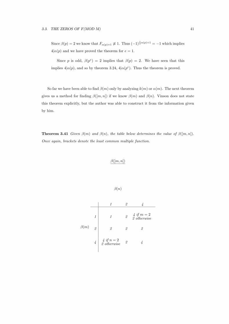
Theorem 3.41 Given β(m) and β(n), the table below determines the value of β([m,n]).
Once again, brackets denote the least common multiple function.
β([m,n])
β(n)
β(m)
1 2 4
1 1 2 4 if m = 22 otherwise
2 2 2 2
4 4 if n = 22 otherwise 2 4
42 CHAPTER 3. MODULAR REPRESENTATIONS OF FIBONACCI SEQUENCES
Proof: Let
α(m) = 2ra β(m) = 2s k(m)2taα(n) = 2wb β(n) = 2x k(n)2yb
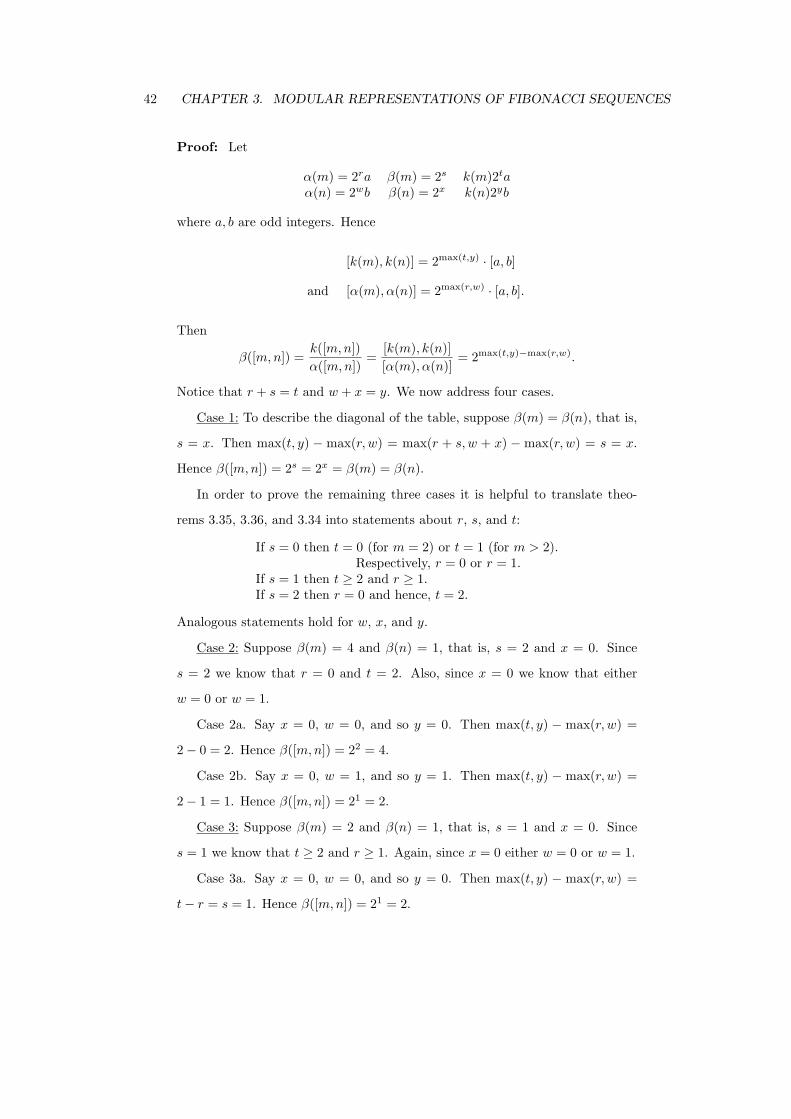
where a, b are odd integers. Hence
[k(m), k(n)] = 2max(t,y) · [a, b]
and [α(m), α(n)] = 2max(r,w) · [a, b].
Then
β([m,n]) =k([m,n])α([m,n])
=[k(m), k(n)][α(m), α(n)]
= 2max(t,y)−max(r,w).
Notice that r + s = t and w + x = y. We now address four cases.
Case 1: To describe the diagonal of the table, suppose β(m) = β(n), that is,
s = x. Then max(t, y) − max(r, w) = max(r + s, w + x) − max(r, w) = s = x.
Hence β([m,n]) = 2s = 2x = β(m) = β(n).
In order to prove the remaining three cases it is helpful to translate theo-
rems 3.35, 3.36, and 3.34 into statements about r, s, and t:
If s = 0 then t = 0 (for m = 2) or t = 1 (for m > 2).Respectively, r = 0 or r = 1.
If s = 1 then t ≥ 2 and r ≥ 1.If s = 2 then r = 0 and hence, t = 2.
Analogous statements hold for w, x, and y.
Case 2: Suppose β(m) = 4 and β(n) = 1, that is, s = 2 and x = 0. Since
s = 2 we know that r = 0 and t = 2. Also, since x = 0 we know that either
w = 0 or w = 1.
Case 2a. Say x = 0, w = 0, and so y = 0. Then max(t, y) − max(r, w) =
2− 0 = 2. Hence β([m,n]) = 22 = 4.
Case 2b. Say x = 0, w = 1, and so y = 1. Then max(t, y) − max(r, w) =
2− 1 = 1. Hence β([m,n]) = 21 = 2.
Case 3: Suppose β(m) = 2 and β(n) = 1, that is, s = 1 and x = 0. Since
s = 1 we know that t ≥ 2 and r ≥ 1. Again, since x = 0 either w = 0 or w = 1.
Case 3a. Say x = 0, w = 0, and so y = 0. Then max(t, y) − max(r, w) =
t− r = s = 1. Hence β([m,n]) = 21 = 2.

3.3. THE ZEROS OF F(MOD M) 43
Case 3b. Say x = 0, w = 1, and so y = 1. Then max(t, y) − max(r, w) =
t− r = s = 1. Hence β([m,n]) = 21 = 2.
Case 4: Suppose β(m) = 4 and β(n) = 2, that is, s = 2 and x = 1. Then
r = 0, t = 2, and w ≥ 1, y ≥ 2. Then max(t, y) −max(r, w) = y − w = x = 1.
Hence β([m,n]) = 21 = 2.
This completes the proof.
There are two interesting corollaries that follow.
Corollary 3.42 If 3|m then β(m) = 2.
Proof: Since β(3) = 2 we know that β(3e) = 2. Let m be expressed as 3en
where 36 | n. By the previous theorem, then β(m) = β([3e, n]) = 2.
Corollary 3.43 β(m) = 1 if and only if 86 |m and α(p) ≡ 2 (mod 4) for all odd primes p
that divide m.
Proof: Let m have the prime factorization m =∏
peii . Suppose β(m) = 1. By
theorem 3.41 it is easy to see that we must have β(peii ) = 1 for all i. If p1 is the
smallest prime in the prime factorization of m and p1 = 2 then by corollary 3.39,
e1 ≤ 2 and thus 8 6 | m. Recall that for odd p, β(peii ) = β(pi). Theorem 3.36
tells us that if α(pi) ≡ 1 or 3 (mod 4) then β(pi) = 4. Theorem 3.34 tells us
that if α(pi) ≡ 0 (mod 4) then β(pi) = 4. Hence when β(m) = 1 we must have
α(pi) ≡ 2 (mod 4) for all i.
Suppose that 8 6 | m. Thus if 2e is a factor of m, then e ≤ 2 and β(2e) = 1.
For odd p, if α(p) ≡ 2 (mod 4) then β(p) = 1 by theorems 3.35 and 3.40. Hence
if we suppose that α(peii ) ≡ 2 (mod 4) for all i we have β(pei
i ) = 1 for all i and
then theorem 3.41 indicates that β(m) = 1.
We now know that for composite m, β(m) can be determined by factoring m into smaller
moduli. We also know that for odd primes p, β(pe) = β(p). Can we determine β(p) for
odd primes p? While k(p) and α(p) have strongly resisted this analysis, we can make some
progress on β(p). The four results are grouped together in the following theorem found in
[21].
44 CHAPTER 3. MODULAR REPRESENTATIONS OF FIBONACCI SEQUENCES
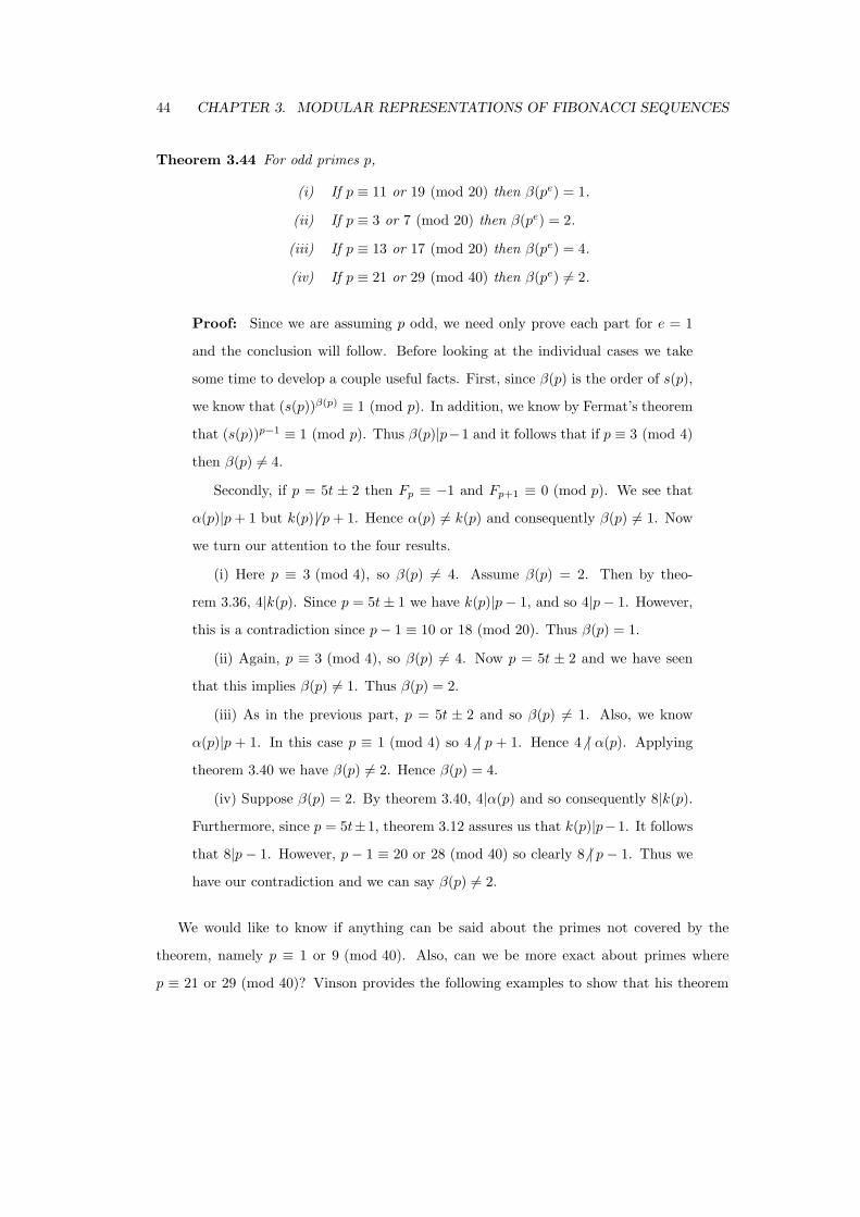
Theorem 3.44 For odd primes p,
(i) If p ≡ 11 or 19 (mod 20) then β(pe) = 1.
(ii) If p ≡ 3 or 7 (mod 20) then β(pe) = 2.
(iii) If p ≡ 13 or 17 (mod 20) then β(pe) = 4.
(iv) If p ≡ 21 or 29 (mod 40) then β(pe) 6= 2.
Proof: Since we are assuming p odd, we need only prove each part for e = 1
and the conclusion will follow. Before looking at the individual cases we take
some time to develop a couple useful facts. First, since β(p) is the order of s(p),
we know that (s(p))β(p) ≡ 1 (mod p). In addition, we know by Fermat’s theorem
that (s(p))p−1 ≡ 1 (mod p). Thus β(p)|p−1 and it follows that if p ≡ 3 (mod 4)
then β(p) 6= 4.
Secondly, if p = 5t ± 2 then Fp ≡ −1 and Fp+1 ≡ 0 (mod p). We see that
α(p)|p + 1 but k(p)6 | p + 1. Hence α(p) 6= k(p) and consequently β(p) 6= 1. Now
we turn our attention to the four results.
(i) Here p ≡ 3 (mod 4), so β(p) 6= 4. Assume β(p) = 2. Then by theo-
rem 3.36, 4|k(p). Since p = 5t± 1 we have k(p)|p− 1, and so 4|p− 1. However,
this is a contradiction since p− 1 ≡ 10 or 18 (mod 20). Thus β(p) = 1.
(ii) Again, p ≡ 3 (mod 4), so β(p) 6= 4. Now p = 5t ± 2 and we have seen
that this implies β(p) 6= 1. Thus β(p) = 2.
(iii) As in the previous part, p = 5t ± 2 and so β(p) 6= 1. Also, we know
α(p)|p + 1. In this case p ≡ 1 (mod 4) so 4 6 | p + 1. Hence 4 6 | α(p). Applying
theorem 3.40 we have β(p) 6= 2. Hence β(p) = 4.
(iv) Suppose β(p) = 2. By theorem 3.40, 4|α(p) and so consequently 8|k(p).
Furthermore, since p = 5t±1, theorem 3.12 assures us that k(p)|p−1. It follows
that 8|p − 1. However, p − 1 ≡ 20 or 28 (mod 40) so clearly 86 | p − 1. Thus we
have our contradiction and we can say β(p) 6= 2.
We would like to know if anything can be said about the primes not covered by the
theorem, namely p ≡ 1 or 9 (mod 40). Also, can we be more exact about primes where
p ≡ 21 or 29 (mod 40)? Vinson provides the following examples to show that his theorem

3.3. THE ZEROS OF F(MOD M) 45
is “complete”:
For p ≡ 1 (mod 40) : β(521) = 1, β(41) = 2, β(761) = 4
For p ≡ 9 (mod 40) : β(809) = 1, β(409) = 2, β(89) = 4
For p ≡ 21 (mod 40) : β(101) = 1, β(61) = 4
For p ≡ 29 (mod 40) : β(29) = 1, β(109) = 4
We finish section 3.3 with a couple of theorems promised at the end of section 3.1. While
they speak to the character of the period, their proofs are made easy by the theory developed
in this section.
Theorem 3.45 (i) If n ≥ 5 is odd then k(Fn) = 4n.
(ii) If n ≥ 4 is even then k(Fn) = 2n.
Proof: We first note that if Fn is used for the modulus, then naturally α(Fn) =
n.
(i) This result follows from the fact that for m ≥ 3, α(m) odd implies β(m) =
4. For n ≥ 5 and odd, Fn ≥ 3 and α(Fn) = n is odd. Thus k(Fn) = 4n.
(ii) Here, α(Fn) = n is even so β(Fn) = 1 or 2. If β(Fn) = 1 then Fn−1 ≡
Fn+1 ≡ 1 (mod Fn). However, F1, F2, F3, . . . , Fn−1 is non decreasing and F3 ≡
2 (mod Fn), hence our contradiction. Therefore, β(Fn) = 2 and k(Fn) = 2n.
Theorem 3.46 (i) If n ≥ 3 is odd then k(Ln) = 2n.
(ii) If n ≥ 2 is even then k(Ln) = 4n.
Proof: First we establish that α(Ln) = 2n. From identity 1.10, FnLn = F2n
which implies F2n ≡ 0 (mod Ln) so certainly α(Ln)|2n. Now if α(Ln) 6= 2n
then α(Ln) ≤ n. In other words, Ln|Ft for some t ≤ n. However, Ln > Ft for
2 ≤ t ≤ n, so clearly Ln6 | Ft. Hence α(Ln) = 2n.
(i)
Fn+1Ln = Fn+1(Fn+1 + Fn−1)
= F 2n+1 + Fn+1Fn−1
= F 2n+1 + F 2
n + (−1)n (by identity 1.8)
= F2n+1 − 1 (by identity 1.7 and n odd)
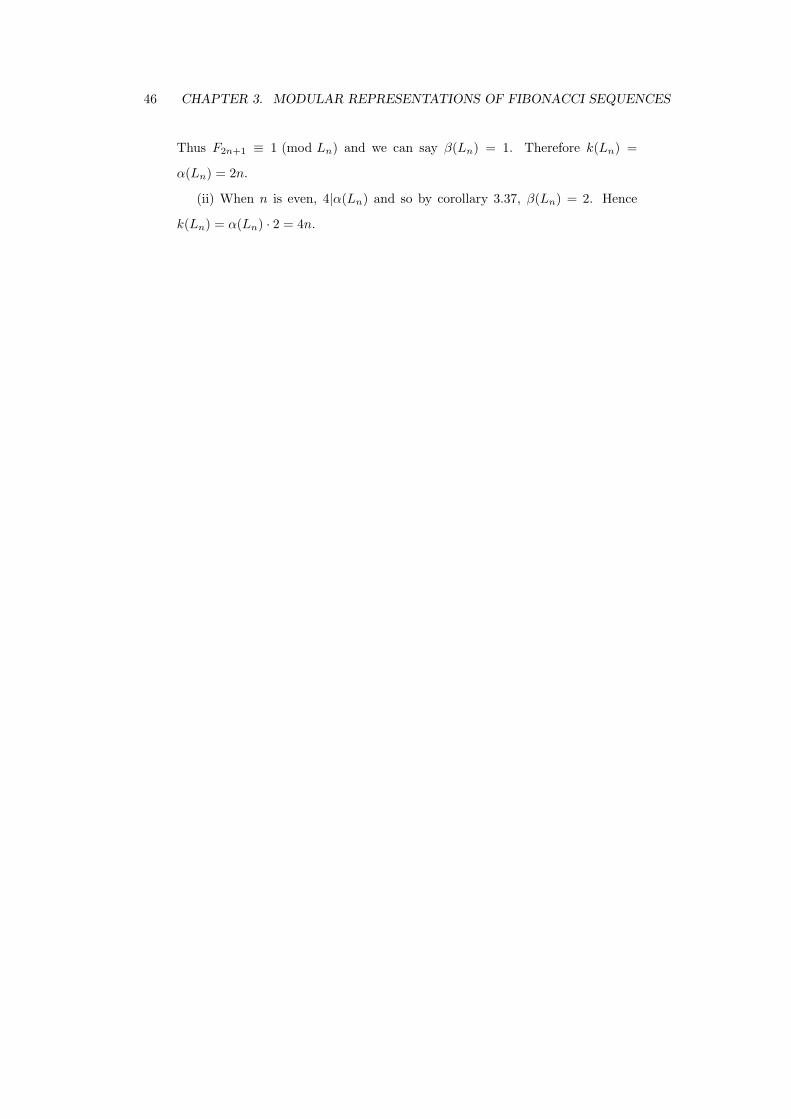
46 CHAPTER 3. MODULAR REPRESENTATIONS OF FIBONACCI SEQUENCES
Thus F2n+1 ≡ 1 (mod Ln) and we can say β(Ln) = 1. Therefore k(Ln) =
α(Ln) = 2n.
(ii) When n is even, 4|α(Ln) and so by corollary 3.37, β(Ln) = 2. Hence
k(Ln) = α(Ln) · 2 = 4n.

Chapter 4
Personal Findings
During my survey of known Fibonacci properties I was fortunate enough to stumble across
a few areas where apparently very little research had been done. Upon examining these
areas more closely I was able to discover yet more astounding properties of the Fibonacci
sequence.
4.1 Spirolaterals And The Fibonacci Sequence
Spirolaterals, invented in 1973 by Frank C. Odds, are simple graphical representations of
finite integer sequences. The rules for creating a spirolateral from a given sequence are
simple, and the spirolateral can easily be drawn on a sheet of ordinary graph paper. Suppose
we have a sequence x1, x2, x3, . . . , xn. To create the spirolateral draw a line from left to
right x1 units long, turn right 90◦, draw a line x2 units long, turn right 90◦ and continue
in this manner. When the end of the sequence has been reached, start over again with x1.
Figure 4.1: Some simple spirolaterals. The circle indicates the starting point.
Eventually, either the line will return to its starting point heading in the initial direction, or
else the pattern will wander off the page. It is known that when n ≡ 1 or 3 (mod 4) then the
spirolateral exhibits 4-fold symmetry. When n ≡ 2 (mod 4) then then spirolateral exhibits
2-fold symmetry, and when n ≡ 0 (mod 4) the spirolateral does not exhibit symmetry and
usually glides off the page in some diagonal direction.
I wrote a short computer program that randomly generated sequences and then drew
47

48 CHAPTER 4. PERSONAL FINDINGS
them as spirolaterals. After playing with the spirolateral program for a while, viewing
hundreds of spirolaterals, I was accustomed to seeing interesting symmetries and curious
patterns fly off the screen at some diagonal. Then, when I used a period of residues of
the Fibonacci sequence under various moduli to generate spirolaterals I was surprised that
typically the results were not symmetric and often did not translate off the screen.
Figure 4.2: Some spirolaterals using Fibonacci residues. Here, F (mod 5) and F (mod 8) areboth asymmetric and nontranslating. Circles indicate starting points.
Apparently, after only one time through the period, the line had returned to the starting
point and was heading in the initial direction. That is, the sum of the lines drawn to the
right equaled the sum of the lines drawn to the left, and the sum of the lines drawn up
equaled the sum of the lines drawn down. This seemed a fairly remarkable occurrence, for
it indicated a truth about the alternating sum of the residues themselves. After studying
many examples, a conjecture was made and eventually a proof was given showing when the
alternating sum will be zero.
In order to express clearly the idea of working with the residues themselves, let us
introduce some notation. Let fn represent the least nonnegative residue of Fn modulo m.
As we would expect, fn = fn+r·k(m) for any integer r. When n is odd, F−n = Fn and so
f−n = fn. When n is even, F−n = −Fn which implies F−n +Fn ≡ 0 (mod m) and so either
f−n = fn = 0 or else f−n + fn = m
Theorem 4.1 4|k(m) if and only if
k(m)2 −1∑i=0
(−1)if2i+1 = 0.
Proof: Let k = k(m) and rewrite the above summation as
f1 − f3 + f5 − · · · − fk−5 + fk−3 − fk−1
= (f1 − fk−1)− (f3 − fk−3) + · · · − (f k2−1 − f k
2 +1).

4.1. SPIROLATERALS AND THE FIBONACCI SEQUENCE 49
First suppose that 4|k. When n is odd fn = f−n = fk−n. Hence each term in
parentheses equals zero, implying the entire summation equals zero.
On the other hand, since fn = fk−n for odd n we know that each parenthe-
sized term must equal zero, and in particular f k2−1 = f k
2 +1. By the recurrence
relation we know then f k2
= 0. Clearly now β(m) 6= 1 and by theorem 3.35 we
can say 4|k.
It turns out that the same conditions do not ensure that the alternating sum of the
evenly subscripted residues will be zero. However, the conditions needed in this case are
not very different. First, though, we need a lemma.
Lemma 4.2 Suppose 4|k(m) for some m and let j be even. If j is a multiple of k(m)2 then
fj = fk−j = 0 otherwise fj + fk−j = m.
Proof: Let k = k(m) and take all congruences (mod m). When j is even
Fk−j ≡ (−1)j+1Fj ≡ −Fj . Thus if Fj 6≡ 0 then fj + fk−j = m. Since 4|k we
know by theorem 3.35 that F k2≡ 0 and consequently if j is a multiple of k
2 then
fj = 0. Also, k− j will be a multiple of k2 so fk−j = 0. Suppose Ft ≡ 0 for some
0 < t < k2 . Then β(m) = 4 and α(m) = t is necessarily odd. Thus the only time
Fj ≡ 0 and j is even is when j is a multiple of k2 . The lemma follows.
Theorem 4.3 If k(m) ≡ 4 (mod 8) then
k(m)2 −1∑i=0
(−1)if2i = 0.
Proof: The summation above is
f0 − f2 + f4 − f6 + · · ·+ fk−4 − fk−2
= f0 − (f2 + fk−2) + (f4 + fk−4)− · · · − (f k2−2 + f k
2 +2) + f k2.
By our lemma f0 = f k2
= 0 and each quantity in parentheses equals m. There
are 12 (k
2 − 2) = k4 − 1 parenthesized terms and since k ≡ 4 (mod 8) we know
k4 − 1 is even. Hence the entire summation is zero.

50 CHAPTER 4. PERSONAL FINDINGS
We can extend our idea of the spirolateral and instead of restricting ourselves to just 90◦
turns we can make spirolaterals with 60◦ turns or 45◦ etc... If 60◦ turns are used, hexagonal
type patterns emerge. Occasionally these pattern will return to their starting place when
F (mod m) for some m is used as the generating sequence. Since every third line is parallel
in these pictures, this result indicates that the alternating sum of every third term in these
sequences is zero, regardless of where we start to take our sum. The following conjecture
expresses this notion.
Conjecture 4.4 If k(m) ≡ 12 (mod 24) and β(m) = 4 for some m, then
k(m)/3−1∑i=0
(−1)if3i+j = 0
for j = 0, 1, 2.
After only a cursory investigation it appears that this conjecture may yield to a proof if
given a couple hours of thought. Also, many times the alternating sum of every fourth, fifth,
and so on, residue in a period equals zero. This area seems to be quite open for research.
After trying for a while to find results pertaining to the summation of the residues
themselves I turned to a related question. If I take the sum (or alternating sum) of every
nth term of the Fibonacci sequence within a period of F (mod m), what will the result be,
modulo m? For example, k(5) = 20, so what is the sum modulo 5 of every fourth term
starting with, say, F2? Or what can I expect of F3 − F8 + F13 − F18 (mod 5)? To this end
the following two identities are vital. The following identity is due to Siler[16].
Identity 4.5 For 0 ≤ j < n and t ≥ 0, we have
t∑i=0
Fni+j =Fnt+n+j − Fj + (−1)j+1Fn−j + (−1)n+1Fnt+j
Ln − 1 + (−1)n+1.
Proof: The identity στ = −1 will be used several times in the proof.
t∑i=0
Fni+j =t∑
i=0
1√5(τni+j − σni+j)

4.1. SPIROLATERALS AND THE FIBONACCI SEQUENCE 51
=1√5
[τ j
t∑i=0
(τn)i − σjt∑
i=0
(σn)i
]
=1√5
[τ j(1− (τn)t+1)
1− τn− σj(1− (σn)t+1)
1− σn
]
=1√5
[τ j(1− σn)− τnt+n+j(1− σn)− σj(1− τn) + σnt+n+j(1− τn)
(1− τn)(1− σn)
]
=1√5
[(τ j − σj) + (−1)j(τn−j − σn−j)− (τnt+n+j − σnt+n+j) + (−1)n(τnt+j − σnt+j)
1 + (τσ)n − (τn + σn)
]
=Fj + (−1)jFn−j − Fnt+n+j + (−1)nFnt+j
1 + (−1)n − Ln.
By multiplying the numerator and denominator by −1 we obtain the identity.
The second identity is similar, but concerns alternating sums. I have been unable to find
this identity published anywhere, and the proof below is due to Fredric Howard.
Identity 4.6 For 0 ≤ j < n and t ≥ 0, we have
t∑i=0
(−1)iFni+j =Fj + (−1)j+1Fn−j + (−1)tFnt+n+j + (−1)t+nFnt+j
1 + (−1)n + Ln.
Proof:
t∑i=0
(−1)iFni+j =t∑
i=0
(−1)i
√5
(τni+j − σni+j)
=1√5
[τ j
t∑i=0
(−τn)i − σjt∑
i=0
(−σn)i
]
=1√5
[τ j(1− (−τn)t+1)
1− (−τn)− σj(1− (−σn)t+1)
1− (−σn)
]
=1√5
[τ j(1 + σn) + (−1)tτnt+n+j(1 + σn)− σj(1 + τn)− (−1)tσnt+n+j(1 + τn)
(1 + τn)(1 + σn)
]

52 CHAPTER 4. PERSONAL FINDINGS
=1√5
(τ j − σj) + (−1)j+1(τn−j − σn−j) +
(−1)t(τnt+n+j − σnt+n+j) + (−1)t+n(τnt+j − σnt+j)1 + (τσ)n + (τn + σn)
=
Fj + (−1)j+1Fn−j + (−1)tFnt+n+j + (−1)t+nFnt+j
1 + (−1)n + Ln.
If we fix n and j and sum up (using either identity) all terms of the form Fni+j within
a single period of the Fibonacci sequence (F0 ≤ Fni+j < Fk(m)) what will the result be? In
particular, for what values of n, j, and m will the sum be congruent to zero modulo m?
We will only consider those n such that n|k(m). We are not especially interested in
looking at, say, every seventh term if the period is not a multiple of seven. When t = k(m)n −1
let S+
n denote the summation of identity 4.5 and let S+/−
n denote the alternating summation
of identity 4.6.
Hence, letting k = k(m),
S+
n =
kn−1∑i=0
Fni+j =Fk+j − Fj + (−1)j+1Fn−j + (−1)n+1Fk−n+j
Ln − 1 + (−1)n+1.
Since Fj ≡ Fk+j (mod m),
S+
n (Ln − 1 + (−1)n+1) ≡ (−1)j+1Fn−j + (−1)n+1Fk−(n−j)
≡ (−1)j+1Fn−j + (−1)n+1+(n−j)+1Fn−j
≡ 0 (mod m).
Quite surprisingly, j has dropped out of our equation and the following is then true for all
j:
Theorem 4.7 If gcd(m,Ln − 1 + (−1)n+1) = 1 then S+
n ≡ 0 (mod m).
We will now look at some examples to demonstrate the surprising results this theorem
gives us.
When n = 1, Ln − 1 + (−1)n+1 = 1, and so for any modulus m, S+
1 ≡ 0 (mod m). In
other words, F0 + F1 + F2 + · · ·+ Fk(m)−1 ≡ 0 (mod m) for all m.
When n = 2, Ln − 1 + (−1)n+1 = 1, and so for any modulus m, S+
2 ≡ 0 (mod m).
Consider n = 4. Here Ln − 1 + (−1)n+1 = 5. Thus if 4|k(m) but 5 6 | m then
S+
4 ≡ 0 (mod m). Recall that this means∑k/4−1
i=0 F4i ≡∑k/4−1
i=0 F4i+1 ≡∑k/4−1
i=0 F4i+2 ≡
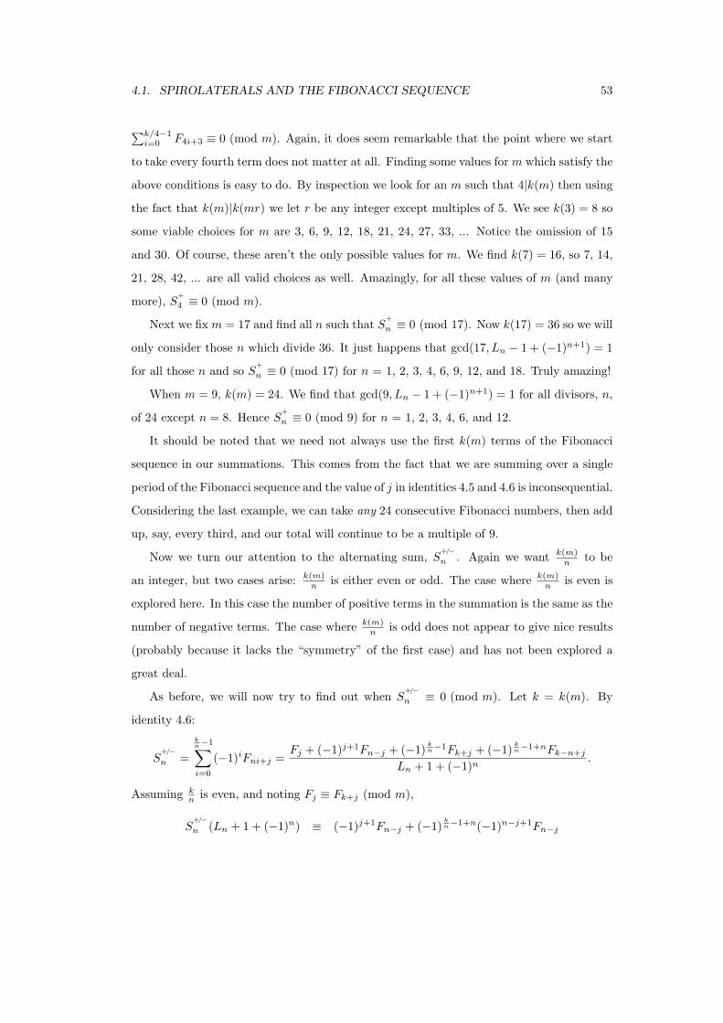
4.1. SPIROLATERALS AND THE FIBONACCI SEQUENCE 53
∑k/4−1i=0 F4i+3 ≡ 0 (mod m). Again, it does seem remarkable that the point where we start
to take every fourth term does not matter at all. Finding some values for m which satisfy the
above conditions is easy to do. By inspection we look for an m such that 4|k(m) then using
the fact that k(m)|k(mr) we let r be any integer except multiples of 5. We see k(3) = 8 so
some viable choices for m are 3, 6, 9, 12, 18, 21, 24, 27, 33, ... Notice the omission of 15
and 30. Of course, these aren’t the only possible values for m. We find k(7) = 16, so 7, 14,
21, 28, 42, ... are all valid choices as well. Amazingly, for all these values of m (and many
more), S+
4 ≡ 0 (mod m).
Next we fix m = 17 and find all n such that S+
n ≡ 0 (mod 17). Now k(17) = 36 so we will
only consider those n which divide 36. It just happens that gcd(17, Ln − 1 + (−1)n+1) = 1
for all those n and so S+
n ≡ 0 (mod 17) for n = 1, 2, 3, 4, 6, 9, 12, and 18. Truly amazing!
When m = 9, k(m) = 24. We find that gcd(9, Ln − 1 + (−1)n+1) = 1 for all divisors, n,
of 24 except n = 8. Hence S+
n ≡ 0 (mod 9) for n = 1, 2, 3, 4, 6, and 12.
It should be noted that we need not always use the first k(m) terms of the Fibonacci
sequence in our summations. This comes from the fact that we are summing over a single
period of the Fibonacci sequence and the value of j in identities 4.5 and 4.6 is inconsequential.
Considering the last example, we can take any 24 consecutive Fibonacci numbers, then add
up, say, every third, and our total will continue to be a multiple of 9.
Now we turn our attention to the alternating sum, S+/−
n . Again we want k(m)n to be
an integer, but two cases arise: k(m)n is either even or odd. The case where k(m)
n is even is
explored here. In this case the number of positive terms in the summation is the same as the
number of negative terms. The case where k(m)n is odd does not appear to give nice results
(probably because it lacks the “symmetry” of the first case) and has not been explored a
great deal.
As before, we will now try to find out when S+/−
n ≡ 0 (mod m). Let k = k(m). By
identity 4.6:
S+/−
n =
kn−1∑i=0
(−1)iFni+j =Fj + (−1)j+1Fn−j + (−1)
kn−1Fk+j + (−1)
kn−1+nFk−n+j
Ln + 1 + (−1)n.
Assuming kn is even, and noting Fj ≡ Fk+j (mod m),
S+/−
n (Ln + 1 + (−1)n) ≡ (−1)j+1Fn−j + (−1)kn−1+n(−1)n−j+1Fn−j

54 CHAPTER 4. PERSONAL FINDINGS
≡ (−1)j+1Fn−j + (−1)jFn−j
≡ 0 (mod m)
Once again j has dropped out and we are left with the following result.
Theorem 4.8 If k(m)n is even and gcd(m,Ln + 1 + (−1)n) = 1 then S
+/−
n ≡ 0 (mod m).
Here are a couple examples of the application of this theorem.
Let n = 4. Then Ln + 1 + (−1)n = 9. Now we want the values for m such that k(m)4
is even and gcd(m, 9) = 1, the latter requirement being the same as 3 6 | m. After some
inspection we find m = 7 works since k(m) = 16. Thus m = 7, 14, 28, 35, 49, ... are all
acceptable values. Also, k(16) = 24 so m = 16, 32, 64, 80, 112, ... work as well. For all
these values of m, S+/−
4 ≡ 0 (mod m).
When m = 9, k(m) = 24. We see that k(m)n is even for n = 1, 2, 3, 4, 6, 12. Of these
values, gcd(9, Ln + 1 + (−1)n) = 1 for n = 1, 2, 3, 6. Hence S+/−
1 ≡ S+/−
2 ≡ S+/−
3 ≡ S+/−
6 ≡
0 (mod 9).
When m = 17, k(m) = 36. Now k(m)n is even for n = 1, 2, 3, 6, 9, 18. Of these values,
gcd(17, Ln + 1 + (−1)n) = 1 for n = 1, 2, 3, 6, 9. Hence S+/−
1 ≡ S+/−
2 ≡ S+/−
3 ≡ S+/−
6 ≡
S+/−
9 ≡ 0 (mod 17).
It is remarkable that in the example above where m = 9, the alternating sum of the
residues themselves for n = 1, 2, 3, and 6 actually equals zero when j 6= 0. When j = 0, the
alternating sum of the residues equals −9 for all four values of n.
Similarly, in the example when m = 17, the alternating sum of the residues themselves
actually equals zero for all j. Clearly this is an area that is wide open for research and
appears to have some fascinating results.
Though we have provided some sufficient conditions indicating when a sum will be
congruent to zero, these conditions are nowhere close to necessary. There are many times
when a sum will be congruent to zero for some j but not all. It appears that with some
work, new and more general sufficient conditions may be found.
The notion of summing Fibonacci numbers over a single period is not new and has been
examined previously by Aydin and Smith in [3]. Their approach, however, was to take the
sum of powers of all the Fibonacci numbers in a period of F (mod p) and observe its value

4.2. FIBONACCI SUBSEQUENCES 55
∑Fi ≡ 0
∑(−1)iFi ≡ 0
For all primes p∑
F 2i ≡ 0∑
F 3i ≡ 0
∑(−1)iF 3
i ≡ 0
For p 6= 3∑
(−1)iF 4i ≡ 0
For p 6= 11∑
F 5i ≡ 0
∑(−1)iF 5
i ≡ 0
For p 6= 11, 29∑
F 6i ≡ 0∑
F 7i ≡ 0
∑(−1)iF 7
i ≡ 0
Table 4.1: Some sums of powers of Fibonacci numbers.
modulo p, where p is a prime. Table 4.1 displays a few of their results. All sums are taken
over a single period and all congruences are (mod p).
It seems that the next step is to look at summations of the form∑
F eni+j and
∑(−1)iF e
ni+j .
While no known work has been done in this area, empirical evidence suggests that there are
many interesting theorems waiting to be proven.
4.2 Fibonacci Subsequences
During my research I came across a paper [8] by Herta Freitag in which she describes
a property of the unit digits of the Fibonacci numbers. In the paper she examines sev-
eral subsequences of F (mod 10) where the terms of the subsequence actually follow the
usual Fibonacci recurrence relation. First she conjectures and proves that Fn + Fn+5 ≡
Fn+10 (mod 10) for all n, then she shows that if j ∈ {1, 5, 13, 17, 25, 29, 37, 41, 49, 53} the
relation Fn + Fn+j ≡ Fn+2j (mod 10) still holds for all n.
Her paper leaves many questions open. Are there other subsequences of this type in
F (mod 10) which do depend on the value of n as defined above? What can we say about the
subsequences of F (mod m) for arbitrary m? We can immediately answer the first question
by noting that F0, F9, F18, . . . (mod 10) forms such a sequence, but F1, F10, F19, . . . (mod 10)
does not. We will examine the second question closely.
First we need some notation. If a subsequence H of F (mod m) exhibits the recurrence
56 CHAPTER 4. PERSONAL FINDINGS
relation Hn+2 ≡ Hn+1 + Hn (mod m), let us call H a “Fibonacci subsequence modulo
m”. We will drop the “modulo m” when the modulus is understood. We will only consider
subsequences whose terms are evenly spaced throughout F (mod m) and we will denote such
subsequence by {Fn, Fn+j} where Fn and Fn+j are successive term of the subsequence. We
will often use the variables n and j like this where Fn is a term in the subsequence and j is
the “spread” of the subsequence. Since F (mod m) has period k(m), we will always assume
0 ≤ n < k(m) and 1 ≤ j ≤ k(m).
Let us examine some properties of these Fibonacci subsequences. Let d =
gcd(j, k(m)). If {Fn, Fn+j} is a Fibonacci subsequence then {Fn+dx, Fn+dx+j} is also a
Fibonacci subsequence for all x. To see this, consider a period of F (mod m) where we start
at Fn then take every jth term. When we reach the end of the period, we “loop” back to the
start and continue. After “wrapping” around once or several times we will eventually return
to Fn. In the process, we will have taken every dth number in the period. Thus not only
is {Fn+dx, Fn+dx+j} a Fibonacci subsequence, in a sense it is the same subsequence with a
different starting point. We say that it is a “rotation” of the subsequence {Fn, Fn+j}.
In particular, notice that if {Fn, Fn+j} is a Fibonacci subsequence and gcd(j, k(m)) = 1,
then {Ft, Ft+j} is a rotation of {Fn, Fn+j} for any t, and the subsequence has k(m) terms.
So how do we find these Fibonacci subsequences? Given only a few successive terms of
{Fn, Fn+j}, can we say whether or not it is a Fibonacci subsequence, without having to
compute the entire subsequence? As a matter of fact, the main result of this section proves
that in many cases we can do just that. Before we present the main result we provide the
following two lemmas.
Lemma 4.9 {F0, Fj} is a Fibonacci subsequence if and only if {Fn, Fn+j} is a Fibonacci
subsequence with Fn ≡ 0.
Proof: The ideas in this proof are similar to those in the proof of theo-
rem 3.25. Let s be the residue of Fn+1 (mod m). The pair (Fn, Fn+1) ≡
s(F0, F1) (mod m), hence the sequence Fn, Fn+1, Fn+2, . . . (mod m) is the same
as the sequence sF0, sF1, sF2, . . . (mod m). Certainly, if {F0, Fj} is a Fibonacci
subsequence then {sF0, sFj} is a Fibonacci subsequence, and hence {Fn, Fn+j}
is a Fibonacci subsequence.

4.2. FIBONACCI SUBSEQUENCES 57
In the other direction, we know that gcd(s,m) = 1, (this is seen in the
remark after identity 3.26) therefore there exists a t such that t(Fn, Fn+1) ≡
(F0, F1) (mod m), and the result follows as before.
Lemma 4.10 For odd j, Fn−j+Fn ≡ Fn+j (mod m) if and only if (Lj−1)Fn ≡ 0 (mod m).
Proof: We make use of identity 2.1, namely Fn+j = LjFn + (−1)j+1Fn−j , in
the first line below.
Fn−j + Fn ≡ Fn+j ⇐⇒ Fn−j + Fn ≡ LjFn + (−1)j+1Fn−j
⇐⇒ Fn ≡ LjFn (since j is odd)
⇐⇒ (Lj − 1)Fn ≡ 0 (mod m).
We are now ready to present the main theorem of this section.
Theorem 4.11 If Fj ≡ F2j (mod m), then {Fn, Fn+j} is a Fibonacci subsequence for all
n such that Fn ≡ 0 (mod m).
Proof: We will look at two cases: j is odd and j is even. In each case we
will show that {F0, Fj} must be a Fibonacci subsequence, then application of
lemma 4.9 will imply the conclusion of the theorem.
Case 1: Suppose j is odd.
In lemma 4.10 we can view (Lj − 1)Fn ≡ 0 (mod m) as a linear congruence
with Fn given and (Lj−1) the variable. The solution set of this linear congruence
is (Lj − 1) ≡ {0, mdn
, 2mdn
, 3mdn
, . . . , (dn−1)mdn
} where dn = gcd(Fn,m). If (Lj − 1) is
congruent to any of the elements in the set, then the linear congruence will be
satisfied. [4, p. 78].
Let n be given. Then
{odd j : Fn−j + Fn ≡ Fn+j}
={
odd j : (Lj − 1) ≡ 0,m
dn,2m
dn,3m
dn, . . . , or
(dn − 1)mdn
}.
We know that Fn|Ftn so we must have gcd(Fn,m)| gcd(Ftn,m). Thus, using
previous notation, dn|dtn. It follows that {0, mdn
, 2mdn
, . . . , (dn−1)mdn
} ⊆ {0, mdtn
, 2mdtn
, . . . , (dtn−1)mdtn
}.

58 CHAPTER 4. PERSONAL FINDINGS
Hence, if j is a solution given n, then j is a solution given any multiple of n. In
other words, if Fn−j + Fn ≡ Fn+j (mod m) then Ftn−j + Ftn ≡ Ftn+j (mod m)
for all t.
In particular, suppose that j is a solution given n = j (this is exactly what
the hypothesis of our theorem supposes). Then F0 + Fj ≡ F2j , Fj + F2j ≡ F3j ,
F2j + F3j ≡ F4j , . . . (mod m). That is, {F0, Fj} is a Fibonacci subsequence.
Case 2: Suppose j is even.
First we look at a necessary condition. If we assume that {F0, Fj} is, in fact,
a Fibonacci subsequence then we must have Fj ≡ F0 + F−j ≡ F−j (mod m).
However, we know from identity 1.3 that for even j, F−j = −Fj , and so we
must conclude that Fj ≡ −Fj (mod m). Thus if m is odd we must have Fj ≡
0 (mod m), and if m is even we have either Fj ≡ 0 or m2 (mod m). Hence, the
only nontrivial case occurs when m is even and Fj ≡ m2 (mod m).
Once again, identity 2.1 states that Fn+j = LjFn + (−1)j+1Fn−j . When we
let n = tj − j we get Ftj = LjF(t−1)j + (−1)j+1F(t−2)j . When t = 2 we get the
familiar identity F2j = LjFj , which implies here, m2 ≡ Lj(m
2 ) (mod m). We use
this relation to simplify the congruences (taken mod m) below.
F3j ≡ LjF2j − Fj
≡ Lj(m
2)− (
m
2) ≡ 0
F4j ≡ LjF3j − F2j
≡ Lj(0)− (m
2) ≡ m
2
F5j ≡ LjF4j − F3j
≡ Lj(m
2)− (0) ≡ m
2...
Hence our subsequence {F0, Fj} = 0, m2 , m
2 , 0, m2 , m
2 , . . . will continue on in
this manner and {F0, Fj} is a Fibonacci subsequence.
Now it is a simple matter to apply lemma 4.9 and see that if Fn ≡ 0 (mod m)
then {Fn, Fn+j} must also be a Fibonacci subsequence.

4.2. FIBONACCI SUBSEQUENCES 59
This result gives us a fairly easy method for finding many of the Fibonacci subsequences
of F (mod m), if any exist. However, this method may actually give us more than that as
the following conjecture asserts.
Conjecture 4.12 If 56 |m then every Fibonacci subsequence contains a zero.
If the above conjecture is true, then our method should give us all the Fibonacci sub-
sequences of F (mod m) when 56 |m. It also appears that every time 5|m there must be at
least one Fibonacci subsequence containing no zeros. This may have something to do with
the fact that the period of the Lucas numbers = k(m) when 56 |m, and 15k(m) when 5|m.
We also make the next conjecture, which tests for the existence of a Fibonacci subse-
quence when we are given four terms in a row and none of them are required to be congruent
to zero modulo m.
Conjecture 4.13 If Fn−j + Fn ≡ Fn+j and Fn + Fn+j ≡ Fn+2j (mod m) then {Fn, Fn+j}
is a Fibonacci subsequence.
Finding just three consecutive terms of a subsequence which exhibit the Fibonacci recur-
rence relation is not sufficient to conclude that the subsequence is a Fibonacci subsequence.
As a counter example we see that F7, F9, F11 are 1, 4, and 5 (mod 6) respectively, but
F13 ≡ 5 (mod 6).
One thing that makes this area of research attractive is that these subsequences appear
quite frequently. Suppose we don’t count rotations as different subsequences, and we don’t
count trivial subsequences of all zeros or the Fibonacci sequence itself. Then for example
we find that F (mod 5) contains 8 Fibonacci subsequences, F (mod 6) contains 11 Fibonacci
subsequences, F (mod 7) contains 1 Fibonacci subsequence, and F (mod 10) contains 39 Fi-
bonacci subsequences. Table 4.2 lists all the “smallest” pairs (n, n+j) for which {Fn, Fn+j}
is a Fibonacci subsequence modulo 10. Note that k(10) = 60 and β(10) = 4.
Finally we mention that not only is the existence of these special subsequences interest-
ing, but how they actually look has its intrigue. We have seen that if a Fibonacci subse-
quence exits with even spread, then it has the form (m2 )·[F (mod 2)]. Every third residue
from F (mod 6) forms a sequence like 2·[F (mod 3)]. Every seventh residue from F (mod 91)
forms a sequence like F (mod 7) multiplied through by 13.

60 CHAPTER 4. PERSONAL FINDINGS
j gcd(j, 60) (n, n + j)1 1 (0,1)5 5 (0,5) (1,6) (2,7) (3,8) (4,9)9 3 (0,9)10 10 (0,10) (5,15)13 1 (0,13)15 15 (0,15)*17 1 (0,17)20 20 (0,20) (5,25) (10,30) (15,45)21 3 (0,21)25 5 (0,25) (1,26) (2,27) (3,28) (4,29)29 1 (0,29)30 30 (0,30)* (15,45)*33 3 (0,33)35 5 (0,35)37 1 (0,37)40 20 (0,40) (5,45) (10,50) (15,55)41 1 (0,41)45 15 (0,45)* (3,48) (6,51) (9,54) (12,57)49 1 (0,49)50 10 (0,50) (5,55)53 1 (0,53)55 5 (0,55)57 3 (0,57)60 60 (0,60)* (15,75)* (30,90)* (45,105)*
Table 4.2: Subsequences of F (mod 10). The subsequences with asterisks are trivial subse-quences, containing only zeros.

4.2. FIBONACCI SUBSEQUENCES 61
Once again, it appears that for every new insight we gain into the Fibonacci sequence,
a multitude of new relationships emerge to amaze and intrigue us.

62 CHAPTER 4. PERSONAL FINDINGS

Appendix A
The First 30 Fibonacci andLucas Numbers
n Fn Ln
1 1 12 1 33 2 4 = 22
4 3 75 5 116 8 = 23 18 = 2 · 32
7 13 298 21 = 3 · 7 479 34 = 2 · 17 76 = 22 · 19
10 55 = 5 · 11 123 = 3 · 4111 89 19912 144 = 24 · 32 322 = 2 · 7 · 2313 233 52114 377 = 13 · 29 843 = 3 · 28115 610 = 2 · 5 · 61 1364 = 22 · 11 · 3116 987 = 3 · 7 · 47 220717 1597 357118 2584 = 23 · 17 · 19 5778 = 2 · 33 · 10719 4181 = 37 · 113 934920 6765 = 3 · 5 · 11 · 41 15127 = 7 · 216121 10946 = 2 · 13 · 421 24476 = 22 · 29 · 21122 17711 = 89 · 199 39603 = 3 · 43 · 30723 28657 64079 = 139 · 46124 46368 = 25 · 32 · 7 · 23 103682 = 2 · 47 · 110325 75025 = 52 · 3001 167761 = 11 · 101 · 16126 121393 = 233 · 521 271443 = 3 · 9048127 196418 = 2 · 17 · 53 · 109 439204 = 22 · 19 · 577928 317811 = 3 · 13 · 29 · 281 710647 = 72 · 1450329 514229 1149851 = 59 · 1948930 832040 = 23 · 5 · 11 · 31 · 61 1860498 = 2 · 32 · 41 · 2521
63

64 APPENDIX A. THE FIRST 30 FIBONACCI AND LUCAS NUMBERS

65
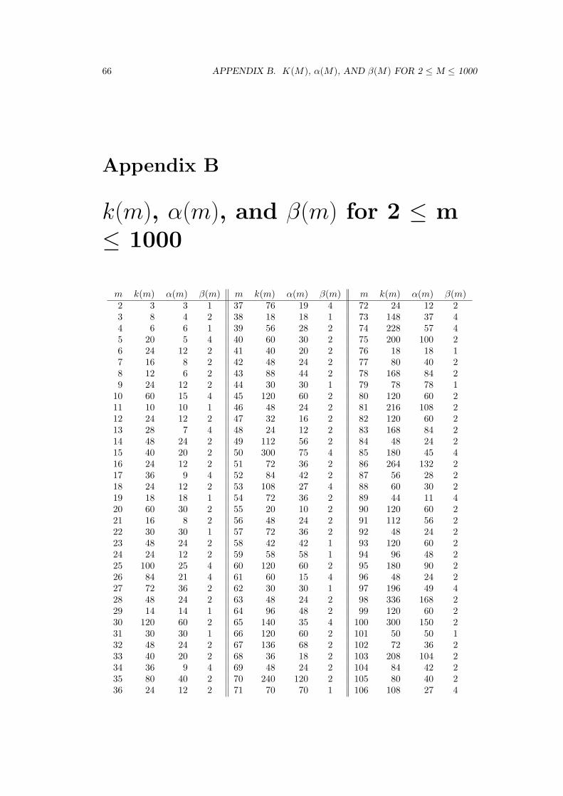
66 APPENDIX B. K(M), α(M), AND β(M) FOR 2 ≤ M ≤ 1000
Appendix B
k(m), α(m), and β(m) for 2 ≤ m≤ 1000
m k(m) α(m) β(m) m k(m) α(m) β(m) m k(m) α(m) β(m)2 3 3 1 37 76 19 4 72 24 12 23 8 4 2 38 18 18 1 73 148 37 44 6 6 1 39 56 28 2 74 228 57 45 20 5 4 40 60 30 2 75 200 100 26 24 12 2 41 40 20 2 76 18 18 17 16 8 2 42 48 24 2 77 80 40 28 12 6 2 43 88 44 2 78 168 84 29 24 12 2 44 30 30 1 79 78 78 1
10 60 15 4 45 120 60 2 80 120 60 211 10 10 1 46 48 24 2 81 216 108 212 24 12 2 47 32 16 2 82 120 60 213 28 7 4 48 24 12 2 83 168 84 214 48 24 2 49 112 56 2 84 48 24 215 40 20 2 50 300 75 4 85 180 45 416 24 12 2 51 72 36 2 86 264 132 217 36 9 4 52 84 42 2 87 56 28 218 24 12 2 53 108 27 4 88 60 30 219 18 18 1 54 72 36 2 89 44 11 420 60 30 2 55 20 10 2 90 120 60 221 16 8 2 56 48 24 2 91 112 56 222 30 30 1 57 72 36 2 92 48 24 223 48 24 2 58 42 42 1 93 120 60 224 24 12 2 59 58 58 1 94 96 48 225 100 25 4 60 120 60 2 95 180 90 226 84 21 4 61 60 15 4 96 48 24 227 72 36 2 62 30 30 1 97 196 49 428 48 24 2 63 48 24 2 98 336 168 229 14 14 1 64 96 48 2 99 120 60 230 120 60 2 65 140 35 4 100 300 150 231 30 30 1 66 120 60 2 101 50 50 132 48 24 2 67 136 68 2 102 72 36 233 40 20 2 68 36 18 2 103 208 104 234 36 9 4 69 48 24 2 104 84 42 235 80 40 2 70 240 120 2 105 80 40 236 24 12 2 71 70 70 1 106 108 27 4
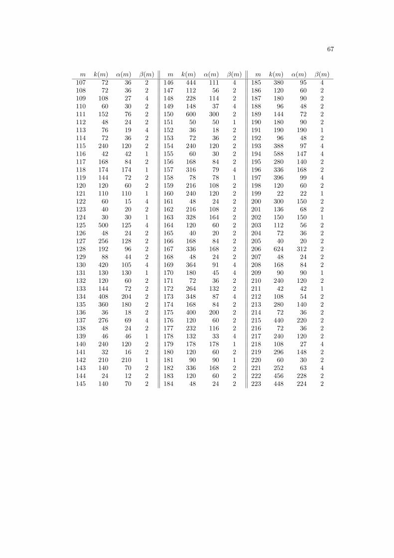
67
m k(m) α(m) β(m) m k(m) α(m) β(m) m k(m) α(m) β(m)107 72 36 2 146 444 111 4 185 380 95 4108 72 36 2 147 112 56 2 186 120 60 2109 108 27 4 148 228 114 2 187 180 90 2110 60 30 2 149 148 37 4 188 96 48 2111 152 76 2 150 600 300 2 189 144 72 2112 48 24 2 151 50 50 1 190 180 90 2113 76 19 4 152 36 18 2 191 190 190 1114 72 36 2 153 72 36 2 192 96 48 2115 240 120 2 154 240 120 2 193 388 97 4116 42 42 1 155 60 30 2 194 588 147 4117 168 84 2 156 168 84 2 195 280 140 2118 174 174 1 157 316 79 4 196 336 168 2119 144 72 2 158 78 78 1 197 396 99 4120 120 60 2 159 216 108 2 198 120 60 2121 110 110 1 160 240 120 2 199 22 22 1122 60 15 4 161 48 24 2 200 300 150 2123 40 20 2 162 216 108 2 201 136 68 2124 30 30 1 163 328 164 2 202 150 150 1125 500 125 4 164 120 60 2 203 112 56 2126 48 24 2 165 40 20 2 204 72 36 2127 256 128 2 166 168 84 2 205 40 20 2128 192 96 2 167 336 168 2 206 624 312 2129 88 44 2 168 48 24 2 207 48 24 2130 420 105 4 169 364 91 4 208 168 84 2131 130 130 1 170 180 45 4 209 90 90 1132 120 60 2 171 72 36 2 210 240 120 2133 144 72 2 172 264 132 2 211 42 42 1134 408 204 2 173 348 87 4 212 108 54 2135 360 180 2 174 168 84 2 213 280 140 2136 36 18 2 175 400 200 2 214 72 36 2137 276 69 4 176 120 60 2 215 440 220 2138 48 24 2 177 232 116 2 216 72 36 2139 46 46 1 178 132 33 4 217 240 120 2140 240 120 2 179 178 178 1 218 108 27 4141 32 16 2 180 120 60 2 219 296 148 2142 210 210 1 181 90 90 1 220 60 30 2143 140 70 2 182 336 168 2 221 252 63 4144 24 12 2 183 120 60 2 222 456 228 2145 140 70 2 184 48 24 2 223 448 224 2

68 APPENDIX B. K(M), α(M), AND β(M) FOR 2 ≤ M ≤ 1000
m k(m) α(m) β(m) m k(m) α(m) β(m) m k(m) α(m) β(m)224 48 24 2 263 176 88 2 302 150 150 1225 600 300 2 264 120 60 2 303 200 100 2226 228 57 4 265 540 135 4 304 72 36 2227 456 228 2 266 144 72 2 305 60 15 4228 72 36 2 267 88 44 2 306 72 36 2229 114 114 1 268 408 204 2 307 88 44 2230 240 120 2 269 268 67 4 308 240 120 2231 80 40 2 270 360 180 2 309 208 104 2232 84 42 2 271 270 270 1 310 60 30 2233 52 13 4 272 72 36 2 311 310 310 1234 168 84 2 273 112 56 2 312 168 84 2235 160 80 2 274 276 69 4 313 628 157 4236 174 174 1 275 100 50 2 314 948 237 4237 312 156 2 276 48 24 2 315 240 120 2238 144 72 2 277 556 139 4 316 78 78 1239 238 238 1 278 138 138 1 317 636 159 4240 120 60 2 279 120 60 2 318 216 108 2241 240 120 2 280 240 120 2 319 70 70 1242 330 330 1 281 56 28 2 320 480 240 2243 648 324 2 282 96 48 2 321 72 36 2244 60 30 2 283 568 284 2 322 48 24 2245 560 280 2 284 210 210 1 323 36 18 2246 120 60 2 285 360 180 2 324 216 108 2247 252 126 2 286 420 210 2 325 700 175 4248 60 30 2 287 80 40 2 326 984 492 2249 168 84 2 288 48 24 2 327 216 108 2250 1500 375 4 289 612 153 4 328 120 60 2251 250 250 1 290 420 210 2 329 32 16 2252 48 24 2 291 392 196 2 330 120 60 2253 240 120 2 292 444 222 2 331 110 110 1254 768 384 2 293 588 147 4 332 168 84 2255 360 180 2 294 336 168 2 333 456 228 2256 384 192 2 295 580 290 2 334 336 168 2257 516 129 4 296 228 114 2 335 680 340 2258 264 132 2 297 360 180 2 336 48 24 2259 304 152 2 298 444 111 4 337 676 169 4260 420 210 2 299 336 168 2 338 1092 273 4261 168 84 2 300 600 300 2 339 152 76 2262 390 390 1 301 176 88 2 340 180 90 2

69
m k(m) α(m) β(m) m k(m) α(m) β(m) m k(m) α(m) β(m)341 30 30 1 380 180 90 2 419 418 418 1342 72 36 2 381 256 128 2 420 240 120 2343 784 392 2 382 570 570 1 421 84 21 4344 264 132 2 383 768 384 2 422 42 42 1345 240 120 2 384 192 96 2 423 96 48 2346 348 87 4 385 80 40 2 424 108 54 2347 232 116 2 386 1164 291 4 425 900 225 4348 168 84 2 387 264 132 2 426 840 420 2349 174 174 1 388 588 294 2 427 240 120 2350 1200 600 2 389 388 97 4 428 72 36 2351 504 252 2 390 840 420 2 429 280 140 2352 240 120 2 391 144 72 2 430 1320 660 2353 236 59 4 392 336 168 2 431 430 430 1354 696 348 2 393 520 260 2 432 72 36 2355 140 70 2 394 396 99 4 433 868 217 4356 132 66 2 395 780 390 2 434 240 120 2357 144 72 2 396 120 60 2 435 280 140 2358 534 534 1 397 796 199 4 436 108 54 2359 358 358 1 398 66 66 1 437 144 72 2360 120 60 2 399 144 72 2 438 888 444 2361 342 342 1 400 600 300 2 439 438 438 1362 90 90 1 401 200 100 2 440 60 30 2363 440 220 2 402 408 204 2 441 336 168 2364 336 168 2 403 420 210 2 442 252 63 4365 740 185 4 404 150 150 1 443 888 444 2366 120 60 2 405 1080 540 2 444 456 228 2367 736 368 2 406 336 168 2 445 220 55 4368 48 24 2 407 380 190 2 446 1344 672 2369 120 60 2 408 72 36 2 447 296 148 2370 1140 285 4 409 408 204 2 448 96 48 2371 432 216 2 410 120 60 2 449 448 224 2372 120 60 2 411 552 276 2 450 600 300 2373 748 187 4 412 624 312 2 451 40 20 2374 180 90 2 413 464 232 2 452 228 114 2375 1000 500 2 414 48 24 2 453 200 100 2376 96 48 2 415 840 420 2 454 456 228 2377 28 14 2 416 336 168 2 455 560 280 2378 144 72 2 417 184 92 2 456 72 36 2379 378 378 1 418 90 90 1 457 916 229 4
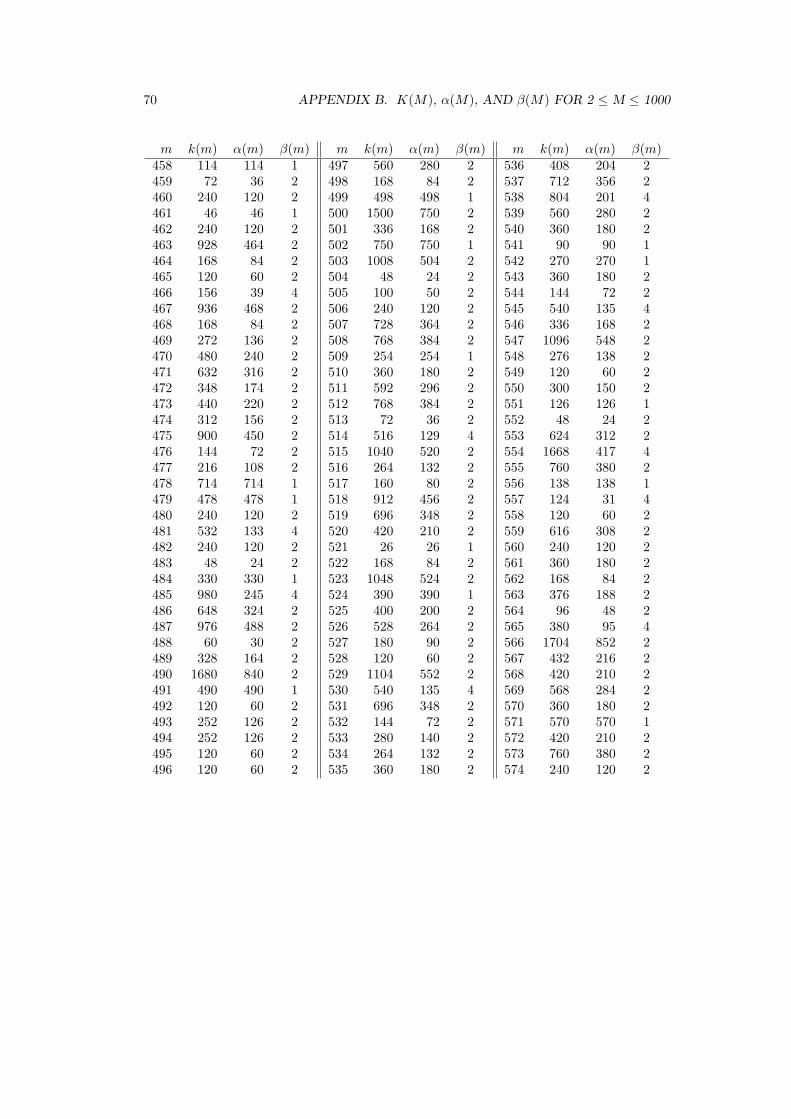
70 APPENDIX B. K(M), α(M), AND β(M) FOR 2 ≤ M ≤ 1000
m k(m) α(m) β(m) m k(m) α(m) β(m) m k(m) α(m) β(m)458 114 114 1 497 560 280 2 536 408 204 2459 72 36 2 498 168 84 2 537 712 356 2460 240 120 2 499 498 498 1 538 804 201 4461 46 46 1 500 1500 750 2 539 560 280 2462 240 120 2 501 336 168 2 540 360 180 2463 928 464 2 502 750 750 1 541 90 90 1464 168 84 2 503 1008 504 2 542 270 270 1465 120 60 2 504 48 24 2 543 360 180 2466 156 39 4 505 100 50 2 544 144 72 2467 936 468 2 506 240 120 2 545 540 135 4468 168 84 2 507 728 364 2 546 336 168 2469 272 136 2 508 768 384 2 547 1096 548 2470 480 240 2 509 254 254 1 548 276 138 2471 632 316 2 510 360 180 2 549 120 60 2472 348 174 2 511 592 296 2 550 300 150 2473 440 220 2 512 768 384 2 551 126 126 1474 312 156 2 513 72 36 2 552 48 24 2475 900 450 2 514 516 129 4 553 624 312 2476 144 72 2 515 1040 520 2 554 1668 417 4477 216 108 2 516 264 132 2 555 760 380 2478 714 714 1 517 160 80 2 556 138 138 1479 478 478 1 518 912 456 2 557 124 31 4480 240 120 2 519 696 348 2 558 120 60 2481 532 133 4 520 420 210 2 559 616 308 2482 240 120 2 521 26 26 1 560 240 120 2483 48 24 2 522 168 84 2 561 360 180 2484 330 330 1 523 1048 524 2 562 168 84 2485 980 245 4 524 390 390 1 563 376 188 2486 648 324 2 525 400 200 2 564 96 48 2487 976 488 2 526 528 264 2 565 380 95 4488 60 30 2 527 180 90 2 566 1704 852 2489 328 164 2 528 120 60 2 567 432 216 2490 1680 840 2 529 1104 552 2 568 420 210 2491 490 490 1 530 540 135 4 569 568 284 2492 120 60 2 531 696 348 2 570 360 180 2493 252 126 2 532 144 72 2 571 570 570 1494 252 126 2 533 280 140 2 572 420 210 2495 120 60 2 534 264 132 2 573 760 380 2496 120 60 2 535 360 180 2 574 240 120 2

71
m k(m) α(m) β(m) m k(m) α(m) β(m) m k(m) α(m) β(m)575 1200 600 2 614 264 132 2 653 1308 327 4576 96 48 2 615 40 20 2 654 216 108 2577 1156 289 4 616 240 120 2 655 260 130 2578 612 153 4 617 1236 309 4 656 120 60 2579 776 388 2 618 624 312 2 657 888 444 2580 420 210 2 619 206 206 1 658 96 48 2581 336 168 2 620 60 30 2 659 658 658 1582 1176 588 2 621 144 72 2 660 120 60 2583 540 270 2 622 930 930 1 661 220 55 4584 444 222 2 623 176 88 2 662 330 330 1585 840 420 2 624 168 84 2 663 504 252 2586 588 147 4 625 2500 625 4 664 168 84 2587 1176 588 2 626 1884 471 4 665 720 360 2588 336 168 2 627 360 180 2 666 456 228 2589 90 90 1 628 948 474 2 667 336 168 2590 1740 870 2 629 684 171 4 668 336 168 2591 792 396 2 630 240 120 2 669 448 224 2592 456 228 2 631 630 630 1 670 2040 1020 2593 1188 297 4 632 156 78 2 671 60 30 2594 360 180 2 633 168 84 2 672 48 24 2595 720 360 2 634 636 159 4 673 1348 337 4596 444 222 2 635 1280 640 2 674 2028 507 4597 88 44 2 636 216 108 2 675 1800 900 2598 336 168 2 637 112 56 2 676 1092 546 2599 598 598 1 638 210 210 1 677 452 113 4600 600 300 2 639 840 420 2 678 456 228 2601 600 300 2 640 960 480 2 679 784 392 2602 528 264 2 641 640 320 2 680 180 90 2603 408 204 2 642 72 36 2 681 456 228 2604 150 150 1 643 1288 644 2 682 30 30 1605 220 110 2 644 48 24 2 683 1368 684 2606 600 300 2 645 440 220 2 684 72 36 2607 1216 608 2 646 36 18 2 685 1380 345 4608 144 72 2 647 1296 648 2 686 2352 1176 2609 112 56 2 648 216 108 2 687 456 228 2610 60 15 4 649 290 290 1 688 264 132 2611 224 112 2 650 2100 525 4 689 756 189 4612 72 36 2 651 240 120 2 690 240 120 2613 1228 307 4 652 984 492 2 691 138 138 1

72 APPENDIX B. K(M), α(M), AND β(M) FOR 2 ≤ M ≤ 1000
m k(m) α(m) β(m) m k(m) α(m) β(m) m k(m) α(m) β(m)692 348 174 2 731 792 396 2 770 240 120 2693 240 120 2 732 120 60 2 771 1032 516 2694 696 348 2 733 1468 367 4 772 1164 582 2695 460 230 2 734 2208 1104 2 773 1548 387 4696 168 84 2 735 560 280 2 774 264 132 2697 360 180 2 736 48 24 2 775 300 150 2698 174 174 1 737 680 340 2 776 588 294 2699 104 52 2 738 120 60 2 777 304 152 2700 1200 600 2 739 738 738 1 778 1164 291 4701 700 175 4 740 1140 570 2 779 360 180 2702 504 252 2 741 504 252 2 780 840 420 2703 684 342 2 742 432 216 2 781 70 70 1704 480 240 2 743 496 248 2 782 144 72 2705 160 80 2 744 120 60 2 783 504 252 2706 708 177 4 745 740 185 4 784 336 168 2707 400 200 2 746 2244 561 4 785 1580 395 4708 696 348 2 747 168 84 2 786 1560 780 2709 118 118 1 748 180 90 2 787 1576 788 2710 420 210 2 749 144 72 2 788 396 198 2711 312 156 2 750 3000 1500 2 789 176 88 2712 132 66 2 751 750 750 1 790 780 390 2713 240 120 2 752 96 48 2 791 304 152 2714 144 72 2 753 1000 500 2 792 120 60 2715 140 70 2 754 84 42 2 793 420 105 4716 534 534 1 755 100 50 2 794 2388 597 4717 952 476 2 756 144 72 2 795 1080 540 2718 1074 1074 1 757 1516 379 4 796 66 66 1719 718 718 1 758 378 378 1 797 228 57 4720 120 60 2 759 240 120 2 798 144 72 2721 208 104 2 760 180 90 2 799 288 144 2722 342 342 1 761 380 95 4 800 1200 600 2723 240 120 2 762 768 384 2 801 264 132 2724 90 90 1 763 432 216 2 802 600 300 2725 700 350 2 764 570 570 1 803 740 370 2726 1320 660 2 765 360 180 2 804 408 204 2727 1456 728 2 766 768 384 2 805 240 120 2728 336 168 2 767 812 406 2 806 420 210 2729 1944 972 2 768 384 192 2 807 536 268 2730 2220 555 4 769 192 96 2 808 300 150 2

73
m k(m) α(m) β(m) m k(m) α(m) β(m) m k(m) α(m) β(m)809 202 202 1 848 216 108 2 887 1776 888 2810 1080 540 2 849 568 284 2 888 456 228 2811 270 270 1 850 900 225 4 889 256 128 2812 336 168 2 851 912 456 2 890 660 165 4813 1080 540 2 852 840 420 2 891 1080 540 2814 1140 570 2 853 1708 427 4 892 1344 672 2815 1640 820 2 854 240 120 2 893 288 144 2816 72 36 2 855 360 180 2 894 888 444 2817 792 396 2 856 72 36 2 895 1780 890 2818 408 204 2 857 1716 429 4 896 192 96 2819 336 168 2 858 840 420 2 897 336 168 2820 120 60 2 859 78 78 1 898 1344 672 2821 820 205 4 860 1320 660 2 899 210 210 1822 552 276 2 861 80 40 2 900 600 300 2823 1648 824 2 862 1290 1290 1 901 108 27 4824 624 312 2 863 1728 864 2 902 120 60 2825 200 100 2 864 144 72 2 903 176 88 2826 1392 696 2 865 1740 435 4 904 228 114 2827 1656 828 2 866 2604 651 4 905 180 90 2828 48 24 2 867 1224 612 2 906 600 300 2829 276 69 4 868 240 120 2 907 1816 908 2830 840 420 2 869 390 390 1 908 456 228 2831 1112 556 2 870 840 420 2 909 600 300 2832 672 336 2 871 952 476 2 910 1680 840 2833 1008 504 2 872 108 54 2 911 70 70 1834 552 276 2 873 1176 588 2 912 72 36 2835 1680 840 2 874 144 72 2 913 840 420 2836 90 90 1 875 2000 1000 2 914 2748 687 4837 360 180 2 876 888 444 2 915 120 60 2838 1254 1254 1 877 1756 439 4 916 114 114 1839 838 838 1 878 438 438 1 917 1040 520 2840 240 120 2 879 1176 588 2 918 72 36 2841 406 406 1 880 120 60 2 919 102 102 1842 84 21 4 881 176 88 2 920 240 120 2843 56 28 2 882 336 168 2 921 88 44 2844 42 42 1 883 1768 884 2 922 138 138 1845 1820 455 4 884 252 126 2 923 140 70 2846 96 48 2 885 1160 580 2 924 240 120 2847 880 440 2 886 888 444 2 925 1900 475 4
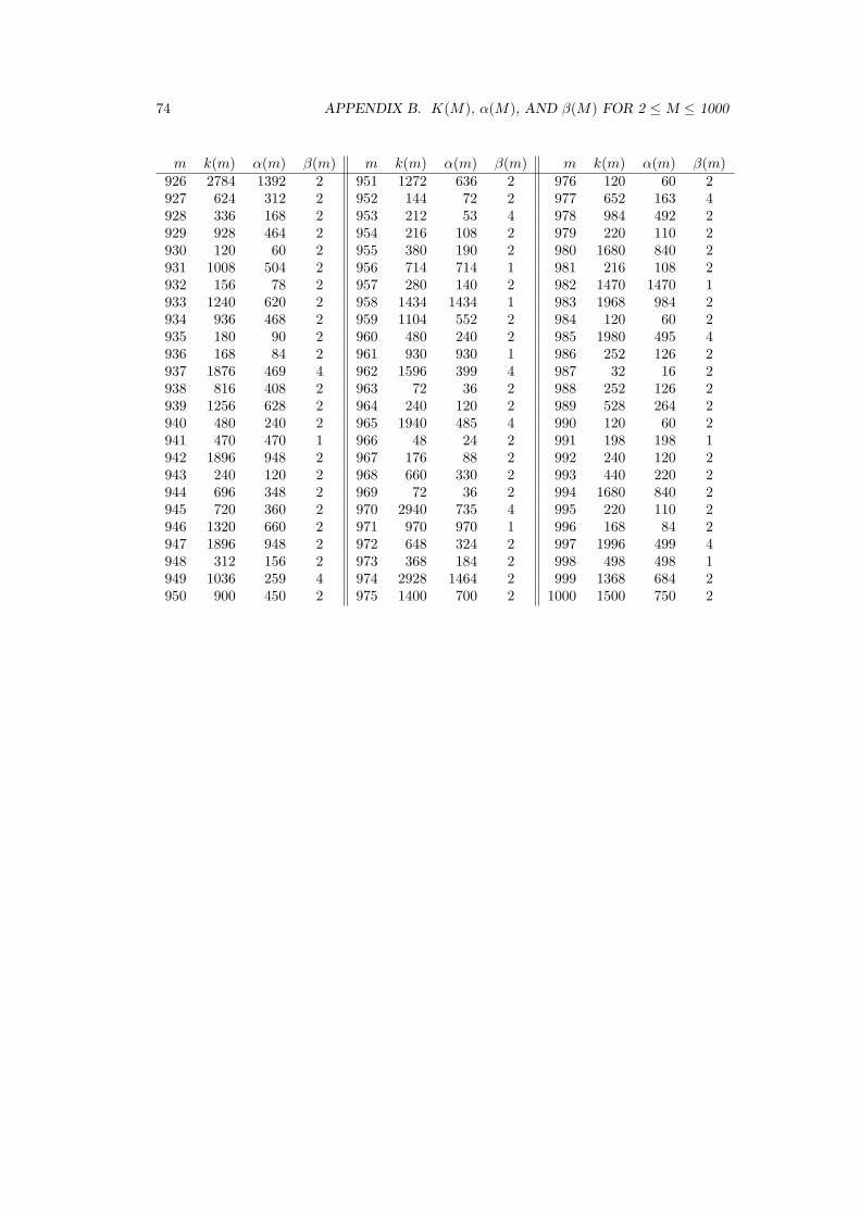
74 APPENDIX B. K(M), α(M), AND β(M) FOR 2 ≤ M ≤ 1000
m k(m) α(m) β(m) m k(m) α(m) β(m) m k(m) α(m) β(m)926 2784 1392 2 951 1272 636 2 976 120 60 2927 624 312 2 952 144 72 2 977 652 163 4928 336 168 2 953 212 53 4 978 984 492 2929 928 464 2 954 216 108 2 979 220 110 2930 120 60 2 955 380 190 2 980 1680 840 2931 1008 504 2 956 714 714 1 981 216 108 2932 156 78 2 957 280 140 2 982 1470 1470 1933 1240 620 2 958 1434 1434 1 983 1968 984 2934 936 468 2 959 1104 552 2 984 120 60 2935 180 90 2 960 480 240 2 985 1980 495 4936 168 84 2 961 930 930 1 986 252 126 2937 1876 469 4 962 1596 399 4 987 32 16 2938 816 408 2 963 72 36 2 988 252 126 2939 1256 628 2 964 240 120 2 989 528 264 2940 480 240 2 965 1940 485 4 990 120 60 2941 470 470 1 966 48 24 2 991 198 198 1942 1896 948 2 967 176 88 2 992 240 120 2943 240 120 2 968 660 330 2 993 440 220 2944 696 348 2 969 72 36 2 994 1680 840 2945 720 360 2 970 2940 735 4 995 220 110 2946 1320 660 2 971 970 970 1 996 168 84 2947 1896 948 2 972 648 324 2 997 1996 499 4948 312 156 2 973 368 184 2 998 498 498 1949 1036 259 4 974 2928 1464 2 999 1368 684 2950 900 450 2 975 1400 700 2 1000 1500 750 2

75

76 APPENDIX C. ONE PERIOD OF F (MOD M) FOR 2 ≤ M ≤ 50
Appendix C
One Period Of F (mod m) for 2≤ m ≤ 50
m2 0 1 13 0 1 1 2 0 2 2 14 0 1 1 2 3 15 0 1 1 2 3 0 3 3 1 4 0 4 4 3 2 0 2 2 4 16 0 1 1 2 3 5 2 1 3 4 1 5 0 5 5 4 3 1 4 5
3 2 5 17 0 1 1 2 3 5 1 6 0 6 6 5 4 2 6 18 0 1 1 2 3 5 0 5 5 2 7 19 0 1 1 2 3 5 8 4 3 7 1 8 0 8 8 7 6 4 1 5
6 2 8 110 0 1 1 2 3 5 8 3 1 4 5 9 4 3 7 0 7 7 4 1
5 6 1 7 8 5 3 8 1 9 0 9 9 8 7 5 2 7 9 65 1 6 7 3 0 3 3 6 9 5 4 9 3 2 5 7 2 9 1
11 0 1 1 2 3 5 8 2 10 112 0 1 1 2 3 5 8 1 9 10 7 5 0 5 5 10 3 1 4 5
9 2 11 113 0 1 1 2 3 5 8 0 8 8 3 11 1 12 0 12 12 11 10 8
5 0 5 5 10 2 12 114 0 1 1 2 3 5 8 13 7 6 13 5 4 9 13 8 7 1 8 9
3 12 1 13 0 13 13 12 11 9 6 1 7 8 1 9 10 5 1 67 13 6 5 11 2 13 1
15 0 1 1 2 3 5 8 13 6 4 10 14 9 8 2 10 12 7 4 110 11 11 7 3 10 13 8 6 14 5 4 9 13 7 5 12 2 14 1
16 0 1 1 2 3 5 8 13 5 2 7 9 0 9 9 2 11 13 8 513 2 15 1
17 0 1 1 2 3 5 8 13 4 0 4 4 8 12 3 15 1 16 0 1616 15 14 12 9 4 13 0 13 13 9 5 14 2 16 1
18 0 1 1 2 3 5 8 13 3 16 1 17 0 17 17 16 15 13 10 515 2 17 1
19 0 1 1 2 3 5 8 13 2 15 17 13 11 5 16 2 18 120 0 1 1 2 3 5 8 13 1 14 15 9 4 13 17 10 7 17 4 1
5 6 11 17 8 5 13 18 11 9 0 9 9 18 7 5 12 17 9 615 1 16 17 13 10 3 13 16 9 5 14 19 13 12 5 17 2 19 1
21 0 1 1 2 3 5 8 13 0 13 13 5 18 2 20 122 0 1 1 2 3 5 8 13 21 12 11 1 12 13 3 16 19 13 10 1
11 12 1 13 14 5 19 2 21 123 0 1 1 2 3 5 8 13 21 11 9 20 6 3 9 12 21 10 8 18
3 21 1 22 0 22 22 21 20 18 15 10 2 12 14 3 17 20 14 112 13 15 5 20 2 22 1
24 0 1 1 2 3 5 8 13 21 10 7 17 0 17 17 10 3 13 16 521 2 23 1
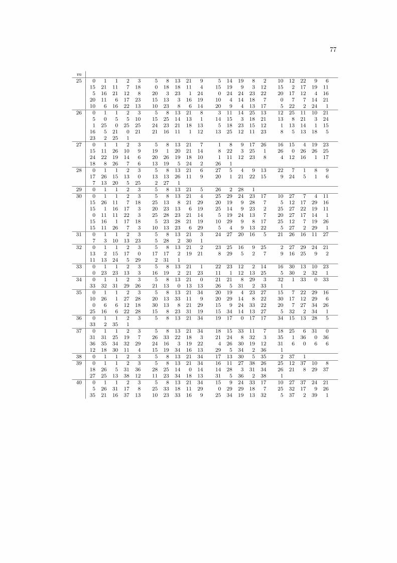
77
m25 0 1 1 2 3 5 8 13 21 9 5 14 19 8 2 10 12 22 9 6
15 21 11 7 18 0 18 18 11 4 15 19 9 3 12 15 2 17 19 115 16 21 12 8 20 3 23 1 24 0 24 24 23 22 20 17 12 4 16
20 11 6 17 23 15 13 3 16 19 10 4 14 18 7 0 7 7 14 2110 6 16 22 13 10 23 8 6 14 20 9 4 13 17 5 22 2 24 1
26 0 1 1 2 3 5 8 13 21 8 3 11 14 25 13 12 25 11 10 215 0 5 5 10 15 25 14 13 1 14 15 3 18 21 13 8 21 3 241 25 0 25 25 24 23 21 18 13 5 18 23 15 12 1 13 14 1 15
16 5 21 0 21 21 16 11 1 12 13 25 12 11 23 8 5 13 18 523 2 25 1
27 0 1 1 2 3 5 8 13 21 7 1 8 9 17 26 16 15 4 19 2315 11 26 10 9 19 1 20 21 14 8 22 3 25 1 26 0 26 26 2524 22 19 14 6 20 26 19 18 10 1 11 12 23 8 4 12 16 1 1718 8 26 7 6 13 19 5 24 2 26 1
28 0 1 1 2 3 5 8 13 21 6 27 5 4 9 13 22 7 1 8 917 26 15 13 0 13 13 26 11 9 20 1 21 22 15 9 24 5 1 67 13 20 5 25 2 27 1
29 0 1 1 2 3 5 8 13 21 5 26 2 28 130 0 1 1 2 3 5 8 13 21 4 25 29 24 23 17 10 27 7 4 11
15 26 11 7 18 25 13 8 21 29 20 19 9 28 7 5 12 17 29 1615 1 16 17 3 20 23 13 6 19 25 14 9 23 2 25 27 22 19 110 11 11 22 3 25 28 23 21 14 5 19 24 13 7 20 27 17 14 1
15 16 1 17 18 5 23 28 21 19 10 29 9 8 17 25 12 7 19 2615 11 26 7 3 10 13 23 6 29 5 4 9 13 22 5 27 2 29 1
31 0 1 1 2 3 5 8 13 21 3 24 27 20 16 5 21 26 16 11 277 3 10 13 23 5 28 2 30 1
32 0 1 1 2 3 5 8 13 21 2 23 25 16 9 25 2 27 29 24 2113 2 15 17 0 17 17 2 19 21 8 29 5 2 7 9 16 25 9 211 13 24 5 29 2 31 1
33 0 1 1 2 3 5 8 13 21 1 22 23 12 2 14 16 30 13 10 230 23 23 13 3 16 19 2 21 23 11 1 12 13 25 5 30 2 32 1
34 0 1 1 2 3 5 8 13 21 0 21 21 8 29 3 32 1 33 0 3333 32 31 29 26 21 13 0 13 13 26 5 31 2 33 1
35 0 1 1 2 3 5 8 13 21 34 20 19 4 23 27 15 7 22 29 1610 26 1 27 28 20 13 33 11 9 20 29 14 8 22 30 17 12 29 60 6 6 12 18 30 13 8 21 29 15 9 24 33 22 20 7 27 34 26
25 16 6 22 28 15 8 23 31 19 15 34 14 13 27 5 32 2 34 136 0 1 1 2 3 5 8 13 21 34 19 17 0 17 17 34 15 13 28 5
33 2 35 137 0 1 1 2 3 5 8 13 21 34 18 15 33 11 7 18 25 6 31 0
31 31 25 19 7 26 33 22 18 3 21 24 8 32 3 35 1 36 0 3636 35 34 32 29 24 16 3 19 22 4 26 30 19 12 31 6 0 6 612 18 30 11 4 15 19 34 16 13 29 5 34 2 36 1
38 0 1 1 2 3 5 8 13 21 34 17 13 30 5 35 2 37 139 0 1 1 2 3 5 8 13 21 34 16 11 27 38 26 25 12 37 10 8
18 26 5 31 36 28 25 14 0 14 14 28 3 31 34 26 21 8 29 3727 25 13 38 12 11 23 34 18 13 31 5 36 2 38 1
40 0 1 1 2 3 5 8 13 21 34 15 9 24 33 17 10 27 37 24 215 26 31 17 8 25 33 18 11 29 0 29 29 18 7 25 32 17 9 26
35 21 16 37 13 10 23 33 16 9 25 34 19 13 32 5 37 2 39 1

78 APPENDIX C. ONE PERIOD OF F (MOD M) FOR 2 ≤ M ≤ 50
m41 0 1 1 2 3 5 8 13 21 34 14 7 21 28 8 36 3 39 1 40
0 40 40 39 38 36 33 28 20 7 27 34 20 13 33 5 38 2 40 142 0 1 1 2 3 5 8 13 21 34 13 5 18 23 41 22 21 1 22 23
3 26 29 13 0 13 13 26 39 23 20 1 21 22 1 23 24 5 29 3421 13 34 5 39 2 41 1
43 0 1 1 2 3 5 8 13 21 34 12 3 15 18 33 8 41 6 4 1014 24 38 19 14 33 4 37 41 35 33 25 15 40 12 9 21 30 8 383 41 1 42 0 42 42 41 40 38 35 30 22 9 31 40 28 25 10 352 37 39 33 29 19 5 24 29 10 39 6 2 8 10 18 28 3 31 34
22 13 35 5 40 2 42 144 0 1 1 2 3 5 8 13 21 34 11 1 12 13 25 38 19 13 32 1
33 34 23 13 36 5 41 2 43 145 0 1 1 2 3 5 8 13 21 34 10 44 9 8 17 25 42 22 19 41
15 11 26 37 18 10 28 38 21 14 35 4 39 43 37 35 27 17 44 1615 31 1 32 33 20 8 28 36 19 10 29 39 23 17 40 12 7 19 260 26 26 7 33 40 28 23 6 29 35 19 9 28 37 20 12 32 44 31
30 16 1 17 18 35 8 43 6 4 10 14 24 38 17 10 27 37 19 1130 41 26 22 3 25 28 8 36 44 35 34 24 13 37 5 42 2 44 1
46 0 1 1 2 3 5 8 13 21 34 9 43 6 3 9 12 21 33 8 413 44 1 45 0 45 45 44 43 41 38 33 25 12 37 3 40 43 37 34
25 13 38 5 43 2 45 147 0 1 1 2 3 5 8 13 21 34 8 42 3 45 1 46 0 46 46 45
44 42 39 34 26 13 39 5 44 2 46 148 0 1 1 2 3 5 8 13 21 34 7 41 0 41 41 34 27 13 40 5
45 2 47 149 0 1 1 2 3 5 8 13 21 34 6 40 46 37 34 22 7 29 36 16
3 19 22 41 14 6 20 26 46 23 20 43 14 8 22 30 3 33 36 207 27 34 12 46 9 6 15 21 36 8 44 3 47 1 48 0 48 48 47
46 44 41 36 28 15 43 9 3 12 15 27 42 20 13 33 46 30 27 835 43 29 23 3 26 29 6 35 41 27 19 46 16 13 29 42 22 15 373 40 43 34 28 13 41 5 46 2 48 1
50 0 1 1 2 3 5 8 13 21 34 5 39 44 33 27 10 37 47 34 3115 46 11 7 18 25 43 18 11 29 40 19 9 28 37 15 2 17 19 365 41 46 37 33 20 3 23 26 49 25 24 49 23 22 45 17 12 29 41
20 11 31 42 23 15 38 3 41 44 35 29 14 43 7 0 7 7 14 2135 6 41 47 38 35 23 8 31 39 20 9 29 38 17 5 22 27 49 2625 1 26 27 3 30 33 13 46 9 5 14 19 33 2 35 37 22 9 3140 21 11 32 43 25 18 43 11 4 15 19 34 3 37 40 27 17 44 115 16 21 37 8 45 3 48 1 49 0 49 49 48 47 45 42 37 29 16
45 11 6 17 23 40 13 3 16 19 35 4 39 43 32 25 7 32 39 2110 31 41 22 13 35 48 33 31 14 45 9 4 13 17 30 47 27 24 125 26 1 27 28 5 33 38 21 9 30 39 19 8 27 35 12 47 9 615 21 36 7 43 0 43 43 36 29 15 44 9 3 12 15 27 42 19 1130 41 21 12 33 45 28 23 1 24 25 49 24 23 47 20 17 37 4 4145 36 31 17 48 15 13 28 41 19 10 29 39 18 7 25 32 7 39 4635 31 16 47 13 10 23 33 6 39 45 34 29 13 42 5 47 2 49 1

Bibliography
[1] Brother U. Alfred, “Primes which are Factors of All Fibonacci Sequences,”Fibonacci Quarterly, 2 (1964), pp. 33-38.
[2] Agnes Andreassian, “Fibonacci Sequences Modulo M,” Fibonacci Quarterly, 12 (1974),pp. 51-64.
[3] Huseyin Aydin and Geoff C. Smith, “Fourier Analysis in Finite Nilpotent Groups,”Applications of Fibonacci Numbers, vol. 5 (1993), pp. 49-59.
[4] David M. Burton, Elementary Number Theory, Third Edition, Wm. C. Brown Pub-lishers, Dubuque, Iowa, 1994.
[5] Paul A. Catlin, “A Lower Bound for the Period of the Fibonacci Series Modulo M,”Fibonacci Quarterly, 12 (1974), pp. 349-350.
[6] Stuart Clary and Paul Hemenway, “On Sums of Cubes of Fibonacci Numbers,”Applications of Fibonacci Numbers, vol. 5 (1993), pp. 123-136.
[7] Amos Ehrlich, “On the Periods of the Fibonacci Sequence Modulo M,”Fibonacci Quarterly, 27 (1989), pp. 11-13.
[8] Herta T. Freitag, “A Property of Unit Digits of Fibonacci Numbers,”Fibonacci Numbers and Their Applications, 1984, pp. 39-41.
[9] John H. Halton, “On the Divisibility Properties of Fibonacci Numbers,”Fibonacci Quarterly, 4 (1966), pp. 217-240.
[10] E. T. Jacobson, “Distribution of the Fibonacci Numbers Mod 2k,” Fibonacci Quarterly,30 (1992), pp. 211-215.
[11] Judy Kramer and Verner E. Hoggatt, Jr., “Special Cases of Fibonacci Periodicity,”Fibonacci Quarterly, 10 (1972), pp. 519-522.
[12] Lawrence Kuipers and Jau-Shyong Shiue, “A Distribution Property of the Sequence ofFibonacci Numbers,” Fibonacci Quarterly, 10 (1972), pp. 375-376, 392.
[13] S. E. Mamangakis,“Remarks on the Fibonacci Series Modulo m,” American Mathematical Monthly, 68(1961), pp. 648-649.
[14] Harald Niederreiter, “Distribution fo the Fibonacci Numbers Mod 5k,”Fibonacci Quarterly, 10 (1972), pp. 373-374.
79

80 BIBLIOGRAPHY
[15] D. W. Robinson, “The Fibonacci Matrix Modulo m,” Fibonacci Quarterly, 1 (1963),pp. 29-36.
[16] Ken Siler “Fibonacci Summations,” Fibonacci Quarterly, 1 (1963), pp. 67-70.
[17] T. E. Stanley, “Some Remarks on the Periodicity of the Sequence of Fibonacci Num-bers,” Fibonacci Quarterly, 14 (1976), pp. 52-54.
[18] T. E. Stanley, “Powers of the Period Function for the Sequence of Fibonacci Numbers,”Fibonacci Quarterly, 18 (1980), pp. 44-45.
[19] T. E. Stanley, “Some Remarks on the Periodicity of the Sequence of Fibonacci Numbers- II,” Fibonacci Quarterly, 18 (1980), pp. 45-47.
[20] Steven Vajda, Fibonacci & Lucas Numbers, and the Golden Section. Ellis HorwoodLimited, Chichester, England, 1989.
[21] John Vinson, “The Relation of the Period Modulo m to the Rand of Apparition of min the Fibonacci Sequence,” Fibonacci Quarterly, 1 (1963), pp. 37-45.
[22] D. D. Wall, “Fibonacci Series Modulo m,” American Mathematical Monthly, 67 (1960),pp. 525-532.