Annual Report - Tulsa Area United Way - Tulsa Area United Way Home


Integral Methods in
Science and Engineering
Techniques and Applications
C. Constanda
S. Potapenko
Editors
Birkhauser
Boston • Basel • Berlin

C. ConstandaUniversity of TulsaDepartment of Mathematical
and Computer Sciences600 South College AvenueTulsa, OK 74104USA
S. PotapenkoUniversity of WaterlooDepartment of Civil
and Environmental Engineering200 University Avenue WestWaterloo, ON N2L 3G1Canada
Cover design by Joseph Sherman, Hamden, CT.
Mathematics Subject Classification (2000): 45-06, 65-06, 74-06, 76-06
Library of Congress Control Number: 2007934436
ISBN-13: 978-0-8176-4670-7 e-ISBN-13: 978-0-8176-4671-4
c©2008 Birkhauser Boston
All rights reserved. This work may not be translated or copied in whole or in part without the written
permission of the publisher (Birkhauser Boston, c/o Springer Science+Business Media LLC, 233
Spring Street, New York, NY 10013, USA) and the author, except for brief excerpts in connection with
reviews or scholarly analysis. Use in connection with any form of information storage and retrieval,
electronic adaptation, computer software, or by similar or dissimilar methodology now known or
hereafter developed is forbidden.
The use in this publication of trade names, trademarks, service marks and similar terms, even if they
are not identified as such, is not to be taken as an expression of opinion as to whether or not they are
subject to proprietary rights.
9 8 7 6 5 4 3 2 1
www.birkhauser.com (IBT)
Contents
Preface . . . . . . . . . . . . . . . . . . . . . . . . . . . . . . . . . . . . . . . . . . . . . . . . . . . . . . . . ix
List of Contributors . . . . . . . . . . . . . . . . . . . . . . . . . . . . . . . . . . . . . . . . . . . xi
1 Superconvergence of Projection Methods for WeaklySingular Integral OperatorsM. Ahues, A. Largillier, A. Amosov . . . . . . . . . . . . . . . . . . . . . . . . . . . . . . . . 1
2 On Acceleration of Spectral Computations for IntegralOperators with Weakly Singular KernelsM. Ahues, A. Largillier, B. Limaye . . . . . . . . . . . . . . . . . . . . . . . . . . . . . . . . . 9
3 Numerical Solution of Integral Equations in Solidificationand Melting with Spherical SymmetryV.S. Ajaev, J. Tausch . . . . . . . . . . . . . . . . . . . . . . . . . . . . . . . . . . . . . . . . . . . . 17
4 An Analytic Solution for the Steady-State Two-Dimensional Advection–Diffusion–Deposition Model by theGILTT ApproachD. Buske, M.T. de Vilhena, D. Moreira, B.E.J. Bodmann . . . . . . . . . . . . . 27
5 Analytic Two-Dimensional Atmospheric PollutantDispersion Simulation by Double GITTM. Cassol, S. Wortmann, M.T. de Vilhena, H.F. de Campos Velho . . . . . 37
6 Transient Acoustic Radiation from a Thin Spherical ElasticShellD.J. Chappell, P.J. Harris, D. Henwood, R. Chakrabarti . . . . . . . . . . . . . . 47
7 The Eigenfrequencies and Mode Shapes of Drilling MastsS. Chergui . . . . . . . . . . . . . . . . . . . . . . . . . . . . . . . . . . . . . . . . . . . . . . . . . . . . . . 55

vi Contents
8 Layer Potentials in Dynamic Bending of ThermoelasticPlatesI. Chudinovich, C. Constanda . . . . . . . . . . . . . . . . . . . . . . . . . . . . . . . . . . . . . 63
9 Direct Methods in the Theory of Thermoelastic PlatesI. Chudinovich, C. Constanda . . . . . . . . . . . . . . . . . . . . . . . . . . . . . . . . . . . . . 75
10 The Dirichlet Problem for the Plane Deformation of aThin Plate on an Elastic FoundationI. Chudinovich, C. Constanda, D. Doty, W. Hamill, S. Pomeranz . . . . . . 83
11 Some Remarks on Homogenization in Perforated DomainsL. Floden, A. Holmbom, M. Olsson, J. Silfver† . . . . . . . . . . . . . . . . . . . . . . 89
12 Dynamic Response of a Poroelastic Half-Space toHarmonic Line TractionsV. Gerasik, M. Stastna . . . . . . . . . . . . . . . . . . . . . . . . . . . . . . . . . . . . . . . . . . . 99
13 Convexity Conditions and Uniqueness and Regularity ofEquilibria in Nonlinear ElasticityS.M. Haidar . . . . . . . . . . . . . . . . . . . . . . . . . . . . . . . . . . . . . . . . . . . . . . . . . . . . . 109
14 The Mathematical Modeling of SyringomyeliaP.J. Harris, C. Hardwidge . . . . . . . . . . . . . . . . . . . . . . . . . . . . . . . . . . . . . . . . 119
15 A System Iterative Method for Solving First-Kind,Degraded Identity Operator EquationsJ. Hilgers, B. Bertram, W. Reynolds . . . . . . . . . . . . . . . . . . . . . . . . . . . . . . . 127
16 Fast Numerical Integration Method Using Taylor SeriesH. Hirayama . . . . . . . . . . . . . . . . . . . . . . . . . . . . . . . . . . . . . . . . . . . . . . . . . . . . 135
17 Boundary Integral Solution of the Two-DimensionalFractional Diffusion EquationJ. Kemppainen, K. Ruotsalainen . . . . . . . . . . . . . . . . . . . . . . . . . . . . . . . . . . . 141
18 About Traces, Extensions, and Co-Normal DerivativeOperators on Lipschitz DomainsS.E. Mikhailov . . . . . . . . . . . . . . . . . . . . . . . . . . . . . . . . . . . . . . . . . . . . . . . . . . . 149
19 On the Extension of Divergence-Free Vector Fields AcrossLipschitz InterfacesD. Mitrea . . . . . . . . . . . . . . . . . . . . . . . . . . . . . . . . . . . . . . . . . . . . . . . . . . . . . . . 161
20 Solutions of the Atmospheric Advection–DiffusionEquation by the Laplace TransformationD.M. Moreira, M.T. de Vilhena, T. Tirabassi, B.E.J. Bodmann . . . . . . . . 171

Contents vii
21 On Quasimodes for Spectral Problems Arising in VibratingSystems with Concentrated MassesE. Perez . . . . . . . . . . . . . . . . . . . . . . . . . . . . . . . . . . . . . . . . . . . . . . . . . . . . . . . . 181
22 Two-Sided Estimates for Local Minimizers in CompressibleElasticityG. Del Piero, R. Rizzoni . . . . . . . . . . . . . . . . . . . . . . . . . . . . . . . . . . . . . . . . . 191
23 Harmonic Oscillations in a Linear Theory of AntiplaneElasticity with MicrostructureS. Potapenko . . . . . . . . . . . . . . . . . . . . . . . . . . . . . . . . . . . . . . . . . . . . . . . . . . . . 201
24 Exterior Dirichlet and Neumann Problems for theHelmholtz Equation as Limits of Transmission ProblemsM.-L. Rapun, F.-J. Sayas . . . . . . . . . . . . . . . . . . . . . . . . . . . . . . . . . . . . . . . . . 207
25 Direct Boundary Element Method with Discretization ofAll Integral OperatorsF.-J. Sayas . . . . . . . . . . . . . . . . . . . . . . . . . . . . . . . . . . . . . . . . . . . . . . . . . . . . . . 217
26 Reciprocity in Elastomechanics: Development of ExplicitResults for Mixed Boundary Value ProblemsA.P.S. Selvadurai . . . . . . . . . . . . . . . . . . . . . . . . . . . . . . . . . . . . . . . . . . . . . . . . 227
27 Integral Equation Modeling of Electrostatic Interactionsin Atomic Force MicroscopyY. Shen, D.M. Barnett, P.M. Pinsky . . . . . . . . . . . . . . . . . . . . . . . . . . . . . . . 237
28 Integral Representation for the Solution of a CrackProblem Under Stretching Pressure in Plane AsymmetricElasticityE. Shmoylova, S. Potapenko, L. Rothenburg . . . . . . . . . . . . . . . . . . . . . . . . . 247
29 Euler–Bernoulli Beam with Energy Dissipation: SpectralProperties and ControlM. Shubov . . . . . . . . . . . . . . . . . . . . . . . . . . . . . . . . . . . . . . . . . . . . . . . . . . . . . . 257
30 Correct Equilibrium Shape Equation of AxisymmetricVesiclesN.K. Vaidya, H. Huang, S. Takagi . . . . . . . . . . . . . . . . . . . . . . . . . . . . . . . . . 267
31 Properties of Positive Solutions of the Falkner–SkanEquation Arising in Boundary Layer TheoryG.C. Yang, L.L. Shi, K.Q. Lan . . . . . . . . . . . . . . . . . . . . . . . . . . . . . . . . . . . . 277
32 Stabilization of a Four-Dimensional System under RealNoise ExcitationJ. Zhu, W.-C. Xie, R.M.C. So . . . . . . . . . . . . . . . . . . . . . . . . . . . . . . . . . . . . . 285
Index . . . . . . . . . . . . . . . . . . . . . . . . . . . . . . . . . . . . . . . . . . . . . . . . . . . . . . . . . . 295
Preface
The international conferences with the generic title of Integral Methods inScience and Engineering (IMSE) are a forum where academics and other re-searchers who rely significantly on (analytic or numerical) integration methodsin their investigations present their newest results and exchange ideas relatedto future projects.
The first two conferences in this series, IMSE1985 and IMSE1990, wereheld at the University of Texas at Arlington under the chairmanship of FredPayne. At the 1990 meeting, the IMSE consortium was created for the purposeof organizing these conferences under the guidance of an International SteeringCommittee. Subsequently, IMSE1993 took place at Tohoku University, Sendai,Japan, IMSE1996 at the University of Oulu, Finland, IMSE1998 at Michi-gan Technological University, Houghton, MI, USA, IMSE2000 in Banff, AB,Canada, IMSE2002 at the University of Saint-Etienne, France, and IMSE2004at the University of Central Florida, Orlando, FL, USA. The IMSE confer-ences have now become recognized as an important platform for scientistsand engineers working with integral methods to contribute directly to the ex-pansion and practical application of a general, elegant, and powerful class ofmathematical techniques.
A remarkable feature of all IMSE conferences is their socially enjoy-able atmosphere of professionalism and camaraderie. Continuing this trend,IMSE2006, organized at Niagara Falls, ON, Canada, by the Department ofCivil and Environmental Engineering and the Department of Applied Mathe-matics of the University of Waterloo, was yet another successful event in thehistory of the IMSE consortium, for which the participants wish to expresstheir thanks to the Local Organizing Committee:
Stanislav Potapenko (University of Waterloo), Chairman;
Peter Schiavone (University of Alberta);
Graham Gladwell (University of Waterloo);
Les Sudak (University of Calgary);
Siv Sivaloganathan (University of Waterloo).
x Preface
The organizers and the participants also wish to acknowledge the financialsupport received from the Faculty of Engineering and the Department of Ap-plied Mathematics, University of Waterloo and the Department of MechanicalEngineering, University of Alberta.
The next IMSE conference will be held in July 2008 in Santander,Spain. Details concerning this event are posted on the conference web page,http://www.imse08.unican.es.
This volume contains 2 invited papers and 30 contributed papers acceptedafter peer review. The papers are arranged in alphabetical order by (first)author’s name.
The editors would like to record their thanks to the referees for their will-ingness to review the papers, and to the staff at Birkhauser-Boston, who havehandled the publication process with their customary patience and efficiency.
Tulsa, Oklahoma, USA Christian Constanda, IMSE Chairman
The International Steering Committee of IMSE:
C. Constanda (University of Tulsa), Chairman
M. Ahues (University of Saint-Etienne)
B. Bertram (Michigan Technological University)
I. Chudinovich (University of Tulsa)
C. Corduneanu (University of Texas at Arlington)
P. Harris (University of Brighton)
A. Largillier (University of Saint-Etienne)
S. Mikhailov (Brunel University)
A. Mioduchowski (University of Alberta)
D. Mitrea (University of Missouri-Columbia)
Z. Nashed (University of Central Florida)
A. Nastase (Rhein.-Westf. Technische Hochschule, Aachen)
F.R. Payne (University of Texas at Arlington)
M.E. Perez (University of Cantabria)
S. Potapenko (University of Waterloo)
K. Ruotsalainen (University of Oulu)
P. Schiavone (University of Alberta, Edmonton)
S. Seikkala (University of Oulu)

List of Contributors
Mario AhuesUniversite de Saint-Etienne23 rue du Docteur Paul Michelon42023 Saint-Etienne, [email protected]
Vladimir AjaevSouthern Methodist University3200 Dyer StreetDallas, TX 75275-0156, [email protected]
Andrey AmosovMoscow Power Engineering Institute(Technical University)Krasnokazarmennaya 14Moscow 111250, [email protected]
David M. BarnettStanford University416 Escondido MallStanford, CA 94305-2205, [email protected]
Barbara S. BertramMichigan Technological University1400 Townsend DriveHoughton, MI 49931-1295, [email protected]
Bardo E.J. BodmannUniversidade Federal do Rio Grandedo SulAv. Osvaldo Aranha 99/4Porto Alegre, RS 90046-900, [email protected]
Daniela BuskeUniversidade Federal do Rio Grandedo SulRua Sarmento Leite 425/3Porto Alegre, RS 90046-900, [email protected]
Haroldo F. de Campos VelhoInstituto Nacional de PesquisasEspaciaisPO Box 515Sao Jose dos Campos, SP 12245-970,[email protected]
Mariana CassolIstituto di Scienze dell’Atmosfera edel ClimaStr. Prov. di Lecce-Monteroni, km1200Lecce I-73100, [email protected]

xii List of Contributors
Roma ChakrabartiUniversity of BrightonLewes RoadBrighton BN2 4GJ, [email protected]
David ChappellUniversity of BrightonLewes RoadBrighton BN2 4GJ, [email protected]
Saıd CherguiEntreprise Nationale des Travauxaux Puits, Direction EngineeringBP 275Hassi-Messaoud 30500, [email protected]
Igor ChudinovichUniversity of Tulsa600 S. College AvenueTulsa, OK 74104-3189, [email protected]
Christian ConstandaUniversity of Tulsa600 S. College AvenueTulsa, OK 74104-3189, [email protected]
Dale R. DotyUniversity of Tulsa600 S. College AvenueTulsa, OK 74104-3189, [email protected]
Liselott FlodenMittuniversitetetAkademigatan 1Ostersund, S-831 25, [email protected]
Vladimir GerasikUniversity of Waterloo200 University Avenue WestWaterloo, ON N2L 3G1, [email protected]
Salim HaidarGrand Valley State University1 Campus DriveAllendale, MI 49401, [email protected]
William HamillUniversity of Tulsa600 S. College AvenueTulsa, OK 74104-3189, [email protected]
Carl HardwidgePrincess Royal HospitalLewes RoadHaywards Heath RH16 4EX, [email protected]
Paul J. HarrisUniversity of BrightonLewes RoadBrighton BN2 4GJ, [email protected]
David HenwoodUniversity of BrightonLewes RoadBrighton BN2 4GJ, [email protected]
John W. HilgersSignature Research, Inc.56905 Calumet AvenueCalumet, MI 49913, [email protected]
Anders HolmbomMittuniversitetetAkademigatan 1Ostersund, S-831 25, [email protected]

List of Contributors xiii
Huaxiong HuangYork University4700 Keele StreetToronto, ON M3J 1P3, [email protected]
Jukka KemppainenUniversity of OuluPO Box 450090550 Oulu, [email protected]
Kunquan LanRyerson University350 Victoria StreetToronto, ON M5B 2K3, [email protected]
Alain LargillierUniversite de Saint-Etienne23 rue du Docteur Paul Michelon42023 Saint-Etienne, [email protected]
Balmohan V. LimayeIndian Institute of TechnologyBombayPowaiMumbai 400076, [email protected]
Sergey E. MikhailovBrunel University West LondonJohn Crank BuildingUxbridge UB8 3PH, [email protected]
Dorina MitreaUniversity of Missouri202 Math Science BuildingColumbia, MO 65211-4100, [email protected]
Davidson M. MoreiraUniversidade Federal de PelotasRua Carlos Barbosa s/nBage, RS 96412-420, [email protected]
Marianne OlssonMittuniversitetetAkademigatan 1Ostersund, S-831 25, [email protected]
M. Eugenia PerezUniversidad de CantabriaAv. de los Castros s/n39005 Santander, [email protected]
Gianpietro Del PieroUniversita di FerraraVia Saragat 1Ferrara 44100, [email protected]
Peter M. PinskyStanford University496 Lomita MallStanford, CA 94305-4040, [email protected]
Shirley PomeranzUniversity of Tulsa600 S. College AvenueTulsa, OK 74104-3189, [email protected]
Stanislav PotapenkoUniversity of Waterloo200 University Avenue WestWaterloo, ON N2L 3G1, [email protected]
Marıa-Luisa RapunUniversidad Politecnica de MadridCardinal Cisneros 3Madrid 28040, [email protected]

xiv List of Contributors
William R. ReynoldsSignature Research, Inc.56905 Calumet AvenueCalumet, MI 49913, USAreynolds@signatureresearchinc.
com
Raffaella RizzoniUniversita di FerraraVia Saragat 1Ferrara 44100, [email protected]
Keijo RuotsalainenUniversity of OuluPO Box 450090550 Oulu, [email protected]
Francisco-Javier SayasUniversidad de ZaragozaCPS Marıa de Luna 3Zaragoza 50018, [email protected]
Patrick SelvaduraiMcGill University817 Sherbrooke Street WestMontreal, QC H3A 2K6, [email protected]
Yongxing ShenStanford University496 Lomita MallStanford, CA 94305-4040, [email protected]
Lili ShiChengdu University of InformationTechnologyXue Fu Road 24, Block 1Chengdu, Sichuan 610225, PR [email protected]
Elena ShmoylovaTufts University200 College AvenueMedford, MA 02155, [email protected]
Marianna ShubovUniversity of New Hampshire33 College RoadDurham, NH 03824, [email protected]
Ronald M.C. SoHong Kong Polytechnic UniversityHung Hom, KowloonHing [email protected]
Marek StastnaUniversity of Waterloo200 University Avenue WestWaterloo, ON N2L 3G1, [email protected]
Shu TakagiUniversity of Tokyo7-3-1 Hongo, Bunkyo-kuTokyo 113-8656, [email protected]
Johannes TauschSouthern Methodist University3200 Dyer StreetDallas, TX 75275-0156, [email protected]
Tiziano TirabassiIstituto di Scienze dell’Atmosfera edel ClimaVia P. Gobetti 101Bologna 40129, Italy
Naveen K. VaidyaYork University4700 Keele StreetToronto, ON M3J 1P3, [email protected]

List of Contributors xv
Marco T. de VilhenaUniversidade Federal do Rio Grandedo SulRua Sarmento Leite 425/3Porto Alegre, RS 90046-900, [email protected]
Sergio WortmannUniversidade Federal do Rio Grandedo SulRua Ramiro Barcelos 2777-SantanaPorto Alegre, RS 90035-007, [email protected]
Wei-Chau XieUniversity of Waterloo
200 University Avenue WestWaterloo, ON N2L 3G1, [email protected]
Guanchong YangChengdu University of InformationTechnologyXue Fu Road 24, Block 1Chengdu, Sichuan 610225, PR [email protected]
Jinyu ZhuUniversity of Waterloo200 University Avenue WestWaterloo, ON N2L 3G1, [email protected]


1
Superconvergence of Projection Methods forWeakly Singular Integral Operators
M. Ahues1, A. Largillier1, and A. Amosov2
1 Universite de Saint-Etienne, France; [email protected],[email protected]
2 Moscow Power Engineering Institute (Technical University), Moscow, Russia;[email protected]
1.1 Introduction
In [AALT05], the authors proposed error bounds for the discretization er-ror corresponding to the Kantorovich projection approximation πhT of a lin-ear, compact, weakly singular integral operator T defined in the functionalLebesgue space Lp(0, τ∗) for some p ∈ [1,+∞]. The equation to be solved isϕ = Tϕ + f , where f is a given function lying in the space Lp(0, τ∗). Here,πh is a family of projections onto the piecewise constant function subspace ofLp(0, τ∗) and it is pointwise convergent to the identity operator. The error es-timates in that article were significant for sufficiently regular grids in the sensethat they grew to infinity if the ratio between the biggest and the smallest stepof the mesh went to zero. In this chapter, we discuss four numerical solutionsbased on such a family of projections. We obtain accurate error estimates thatare independent of the length τ∗ of the interval where f and the solution ϕare defined, and we suggest global superconvergence phenomena in the senseof [Sloa82]. Particular attention is given to the transfer equation occurring inastrophysical mathematical models of stellar atmospheres. In that context, τ∗represents the optical depth of the star’s atmosphere and the operator T hasa multiplicative factor ω0 representing the albedo. The error bounds are givenexplicitly in terms of this parameter.
1.2 General Facts
We state the problem in the following terms: Given τ∗ > 0, ω0 ∈ [0, 1[, g suchthat

2 M. Ahues, A. Largillier, and A. Amosov
g(0+) = +∞,
g is continuous, positive and decreasing on ]0,∞[,
g ∈ Lr(R) ∩W 1,r(δ,+∞) for all r ∈ [1,∞[ and all δ > 0,
‖g‖L1(R+) ≤ 12 ,
and a function f , find a function ϕ such that
ϕ(τ) = ω0
∫ τ∗
0
g(|τ − τ ′|)ϕ(τ ′) dτ ′ + f(τ), τ ∈ [0, τ∗].
As an example, we consider the transfer equation
ϕ(τ) =ω0
2
∫ τ∗
0
E1(|τ − τ ′|)ϕ(τ ′) dτ ′ + f(τ), τ ∈ [0, τ∗],
where
E1(τ) :=
∫ 1
0
µ−1e−τ/µ dµ, τ > 0,
the source term f belongs to L1(0, τ∗), the optical depth τ∗ is a very largenumber, and the albedo ω0 may be very close to 1. For details, see [Busb60].
The goal of this chapter is as follows: For a class of four numerical solutionsbased on projections, find accurate error estimates that
1. are independent of the grid regularity,2. are independent of τ∗,3. depend on ω0 in an explicit way,4. suggest global superconvergence phenomena in the sense of [Sloa82].
As an abstract framework for the subsequent development, we choose thefollowing: Set
(Λϕ)(τ) :=
∫ τ∗
0
g(|τ − τ ′|)ϕ(τ ′) dτ ′, τ ∈ [0, τ∗],
and let X and Y be suitable Banach spaces. The problem reads as follows:For f ∈ Y , find ϕ ∈ X such that
ϕ = ω0Λϕ+ f.
We remark that
‖(I − ω0Λ)−1‖ ≤ γ0 :=1
1 − ω0
,
where the equality is attained for X = Y = L2(0,∞).

1 Superconvergence of Projection Methods 3
1.3 Projection Approximations
We consider a family of projections onto piecewise constant functions. Let bea grid of n+ 1 points in [0, τ∗] :
0 =: τ0 < τ1 < . . . < τn−1 < τn := τ∗,
and define
hi := τi − τi−1, i ∈ [[1, n ]],
h := (h1, h2, . . . , hn),
Gh := (τ0, τ1, . . . , τn),
h := maxi∈[[1,n ]]
hi,
Ii− 12
:= ]τi−1, τi[, i ∈ [[1, n ]],
τi− 12
:= (τi−1 + τi)/2, i ∈ [[1, n ]].
The approximating space Ph0(0, τ∗) is characterized by
f ∈ Ph0(0, τ∗) ⇐⇒ ∀i ∈ [[1, n ]], ∀τ ∈ Ii− 1
2, f(τ) = f(τi− 1
2).
In what follows,
p ∈ [1,+∞] := [1,+∞[ ∪ +∞
is arbitrary but fixed once for all.The family of projections
πh : Lp(0, τ∗) → Lp(0, τ∗)
is defined as follows:For all i ∈ [[1, n ]] and all τ ∈ Ii− 1
2,
(πhϕ)(τ) :=1
hi
∫ τi
τi−1
ϕ(τ ′) dτ ′.
Henceπh(Lp(0, τ∗)) = P
h0(0, τ∗).
Four approximations based on πh are considered:
1. The classical Galerkin approximation ϕGh , which solves
ϕGh = ω0πhΛϕ
Gh + πhf.
2. The Sloan approximation ϕSh (iterated Galerkin), which solves
ϕSh = ω
0Λπhϕ
Sh + f.

4 M. Ahues, A. Largillier, and A. Amosov
3. The Kantorovich approximation ϕKh , which solves
ϕKh = ω0πhΛϕ
Kh + f.
4. The authors’ approximation ϕAh (iterated Kantorovich), which solves
ϕAh = ω0Λπhϕ
Ah + f + ω0Λ(I − πh)f.
Remark 1. The following relationships and facts are important and easy tocheck:
ϕGh ∈ P
h0(0, τ∗).
ϕGh is computed through an algebraic linear system.
ϕSh = ω0Λϕ
Gh + f.
If ψh = ω0πhΛψh + πhΛf, then ϕK
h = ω0ψh + f.
If φh = ω0Λπhφh + Λf, then ϕAh = ω0φh + f.
1.4 Superconvergence
Superconvergence is understood with respect to dist(ϕ,Ph0(0, τ∗)).
Theorem 1. In any Hilbert space setting, there exists α such that
‖ϕ− πhϕ‖ ≤ ‖εGh ‖ ≤ α‖ϕ− πhϕ‖.
We now present some useful technical notions and the main result. Define
∆ǫg(τ) := g(τ + ǫ) − g(τ),
ωr(g, δ) := sup0<ǫ≤δ
‖∆ǫg(| · |)‖Lr(R),
ω∞(g, δ) := essup|τ−τ ′|≤δ
|g(τ) − g(τ ′)|,
and for α ∈ [0, 1] and i ∈ [[1, n ]]:
∆hαf(τ) :=
∆αhi
f(τ) for τ ∈ [τi−1, τi − αhi],0 for τ ∈ ]τi − αhi, τi],
ωp(f,Gh) := 21p
[ ∫ 1
0
‖∆hαf‖p
pdα] 1
p
,
ωp(g,Gh) := sup0<τ ′<τ∗
ωp(g(| · −τ ′|,Gh) for p∈ [1,∞[,
ω∞(f,Gh) := maxi∈[[1,n ]]
essupτ,τ ′∈ I
i−12
|f(τ)−f(τ ′)|.
For N ∈ G,K,S,A, we consider the absolute discretization error
εNh := ϕNh − ϕ.
The main result is as follows.

1 Superconvergence of Projection Methods 5
Theorem 2. If 0 = f ∈ Lp(0, τ∗) for some p ∈ [1,+∞], then a unique so-lution ϕ exists and satisfies 0 = ϕ ∈ Lp(0, τ∗). Moreover, the discretizationerrors are such that
‖εKh ‖p
‖ϕ‖p
≤ 4 · 31pω0γ0
∫ h
0
g(τ) dτ,
‖εSh‖p
‖ϕ‖p
≤ 12 · 3− 1pω0γ0
∫ h
0
g(τ) dτ,
‖εAh ‖p
‖ϕ‖p
≤ 48ω20γ0
[ ∫ h
0
g(τ) dτ]2.
A proof of this result may be given considering four steps:
1. Establish the following estimate:For all f ∈ Lp(0, τ∗),
‖(I − πh)f‖p
≤ ωp(f,Gh).
The proof is technical.Let f ∈ Lp(0, τ∗). For all i ∈ [[1, n ]] and τ ∈ Ii−1/2,
(I − πh)f(τ) =1
hi
τi∫
τi−1
(f(τ) − f(τ ′)) dτ ′.
If p < ∞, then
τi∫
τi−1
|(I − πh)f(τ)|p dτ ≤τi∫
τi−1
[ 1
hi
τi∫
τi−1
|f(τ ′) − f(τ)| dτ ′]pdτ
≤ 1
hi
τi∫
τi−1
[ τi∫
τi−1
|f(τ ′) − f(τ)|pdτ ′]dτ
=2
hi
τi∫
τi−1
[ τi∫
τ
|f(τ ′) − f(τ)|pdτ ′]dτ
= 2
τi∫
τi−1
[ (τi−τ)/hi∫
0
|f(τ + αhi) − f(τ)|pdα]dτ
= 2
1∫
0
[ τi−αhi∫
τi−1
|∆αhif(τ)|pdτ
]dα.
As a consequence,

6 M. Ahues, A. Largillier, and A. Amosov
‖(I − πh)f‖pp
≤ 2
n∑
i=1
1∫
0
[ τi−αhi∫
τi−1
|∆αhif(τ)|pdτ ′
]dα = ωp(f,Gh)p.
If p = ∞, the proof is elementary.2. Show that
‖εKh ‖p
‖ϕ‖p
≤ ‖(I − πh)Λ‖p,
‖εSh‖p
‖ϕ‖p
≤ ‖Λ(I − πh)‖p,
‖εAh ‖p
‖ϕ‖p
≤ ‖Λ(I − πh)Λ‖p.
3. Prove that
‖(I − πh)Λ‖p
≤ ω1(g, h)1− 1p ω1(g,Gh)
1p ,
‖Λ(I − πh)‖p
≤ ω1(g, h)1p ω1(g,Gh)1− 1
p ,
‖Λ(I − πh)Λ‖p
≤ ω1(g, h)ω1(g,Gh).
4. Demonstrate that
ω1(g, h) ≤ 4
∫ h
0
g(τ) dτ,
ω1(g,Gh) ≤ 12
∫ h
0
g(τ) dτ.
Remark 2. If the kernel is g := 12E1, then, as h → 0+,
∫ h
0
g(τ) dτ = O(h ln h).
1.5 Numerical Evidence
Let us consider the following data:
1. The kernel: g := 12E1.
2. The albedo: ω0 = 0.5.3. The optical depth: τ∗ = 500.4. A constant source term: f(τ) = 0.5 for all τ ∈ [0, τ∗].5. The number of grid points: n = 1000.6. The first 5 points equally spaced by 0.1.7. The last 5 points equally spaced by 0.1.

1 Superconvergence of Projection Methods 7
8. A uniform grid with 990 points between 0.5 and 499.5 so
h = 0.504.
Figure 1.1 shows the residual functions
Nh := ϕN
h − ω0ΛϕNh − f, N ∈ K,A,
in the subinterval [0, 5] of the whole atmosphere [0, 500].
Since in any normed linear context the relative residuals‖N
h ‖‖f‖ are of the
order of the relative errors‖εNh ‖‖ϕ‖ , the numerical results show that the theo-
retical majorizations are sharp enough.
0
0.5E-3
1.0E-3
1.5E-3
0 1 2 3 4 5
•
•
•••
•
•
•
•• • • • •
×
××××
×
×
×× × × × × ×
Kantorovich Residual •Authors Residual ×
Fig. 1.1. Plotting residuals on [0, 5].
References
[AALT05] Ahues, M., Amosov, A., Largillier, A., Titaud, O.: Lp error estimatesfor projection approximations. Appl. Math. Lett., 18, 381–386 (2005).
[Busb60] Busbridge, I.W.: The Mathematics of Radiative Transfer, CambridgeUniversity Press, Cambridge New York (1960).
[Sloa82] Sloan, I.H.: Superconvergence and the Galerkin method for integralequations of the second kind. In: Treatment of Integral Equations byNumerical Methods, Academic Press, New York, 197–206 (1982).


2
On Acceleration of Spectral Computations forIntegral Operators with Weakly SingularKernels
M. Ahues1, A. Largillier1, and B. Limaye2
1 Universite de Saint-Etienne, France; [email protected],[email protected]
2 Indian Institute of Technology Bombay, Mumbai, India; [email protected]
2.1 Introduction
Let T be a compact integral operator on a Banach space X over the complexscalars C. Consider the eigenvalue problem for T of finding a nonzero ϕ ∈ Xand a nonzero λ ∈ C such that Tϕ = λϕ. More generally, we may considerthe spectral subspace problem for T of finding linearly independent elementsϕ1, . . . , ϕm in X and a nonsingular m × m matrix Θ with complex entriessuch that
[Tϕ1, . . . , Tϕm] = [ϕ1, . . . , ϕm]Θ.
Here, Θ represents the restricted operator TM : M → M , x → Tx, whereM := Span [ϕ1, . . . , ϕm]. If M is the spectral subspace corresponding to aisolated spectral value λ of T , then the spectrum of Θ is λ and m is thealgebraic multiplicity of λ.
If we let X = X1×m and ϕ = [ϕ1, . . . , ϕm] ∈ X, then the above equationcan be written as T ϕ = ϕΘ. Since finding exact solutions of such problems
is a tall order, one often finds an approximation T of T and attempts tosolve the problem T ϕ = ϕ Θ. If an approximate solution (ϕ, Θ) is not suf-ficiently accurate, one may employ an iterative refinement technique or usean acceleration technique as described in Chapter 3 of [ALL01] for improvingthe accuracy. In this procedure, the question of implementation of these tech-niques on a computer is of paramount importance. For this purpose, we mustbe able to reduce this procedure to (finite-dimensional) matrix computations.
If the approximating operator T is of finite rank, then the spectral subspaceproblem T ϕ = ϕ Θ as well as iterative refinement and acceleration can in factbe reduced to matrix computations (see Chapter 5 of [ALL01]).
If X := C0([0, 1],C), the space of all complex-valued continuous functionson the interval [0, 1], and if the kernel of a compact integral operator T on Xis weakly singular, then one may resort to singularity subtraction (see [Ans81]
10 M. Ahues, A. Largillier, and B. Limaye
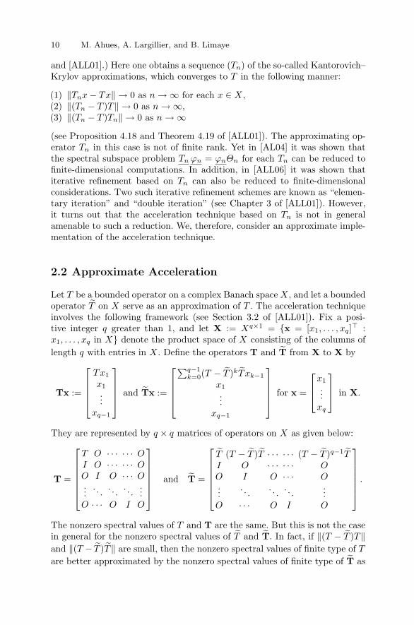
and [ALL01].) Here one obtains a sequence (Tn) of the so-called Kantorovich–Krylov approximations, which converges to T in the following manner:
(1) ‖Tnx− Tx‖ → 0 as n → ∞ for each x ∈ X,(2) ‖(Tn − T )T‖ → 0 as n → ∞,(3) ‖(Tn − T )Tn‖ → 0 as n → ∞
(see Proposition 4.18 and Theorem 4.19 of [ALL01]). The approximating op-erator Tn in this case is not of finite rank. Yet in [AL04] it was shown thatthe spectral subspace problem Tn ϕn = ϕnΘn for each Tn can be reduced tofinite-dimensional computations. In addition, in [ALL06] it was shown thatiterative refinement based on Tn can also be reduced to finite-dimensionalconsiderations. Two such iterative refinement schemes are known as “elemen-tary iteration” and “double iteration” (see Chapter 3 of [ALL01]). However,it turns out that the acceleration technique based on Tn is not in generalamenable to such a reduction. We, therefore, consider an approximate imple-mentation of the acceleration technique.
2.2 Approximate Acceleration
Let T be a bounded operator on a complex Banach space X, and let a boundedoperator T on X serve as an approximation of T . The acceleration techniqueinvolves the following framework (see Section 3.2 of [ALL01]). Fix a posi-tive integer q greater than 1, and let X := Xq×1 = x = [x1, . . . , xq]
⊤ :x1, . . . , xq in X denote the product space of X consisting of the columns of
length q with entries in X. Define the operators T and T from X to X by
Tx :=
⎡⎢⎢⎢⎣
Tx1
x1
...xq−1
⎤⎥⎥⎥⎦ and Tx :=
⎡⎢⎢⎢⎣
∑q−1k=0(T − T )kT xk−1
x1
...xq−1
⎤⎥⎥⎥⎦ for x =
⎡⎢⎣x1
...xq
⎤⎥⎦ in X.
They are represented by q × q matrices of operators on X as given below:
T =
⎡⎢⎢⎢⎢⎢⎣
T O · · · · · · OI O · · · · · · OO I O · · · O...
. . .. . .
. . ....
O · · · O I O
⎤⎥⎥⎥⎥⎥⎦
and T =
⎡⎢⎢⎢⎢⎢⎣
T (T − T )T · · · · · · (T − T )q−1TI O · · · · · · OO I O · · · O...
. . .. . .
. . ....
O · · · O I O
⎤⎥⎥⎥⎥⎥⎦.
The nonzero spectral values of T and T are the same. But this is not the casein general for the nonzero spectral values of T and T. In fact, if ‖(T − T )T‖and ‖(T − T )T‖ are small, then the nonzero spectral values of finite type of T
are better approximated by the nonzero spectral values of finite type of T as

2 Acceleration of Spectral Computations 11
compared with those of T . Also, a basis for a spectral subspace of T is betterapproximated by the first components of a basis for the corresponding spectralsubspace of T. However, if X is infinite-dimensional, then T is not of finiterank (even if T is of finite rank) and it may not be possible to implement the
spectral calculations for T on a computer. This is the case, in general, when Tis a weakly singular integral operator on C0([0, 1],C) and T is a Kantorovich–Krylov approximation of T . In such a situation, we may attempt to employthe iterative refinement technique based on the operator S : X → X given by
S :=
⎡⎢⎢⎢⎢⎢⎣
T O · · · · · · OI O · · · · · · OO I O · · · O...
. . .. . .
. . ....
O · · · O I O
⎤⎥⎥⎥⎥⎥⎦
to obtain approximations of spectral values and spectral subspaces of T. Inthis connection, we prove the following result.
Theorem 1. Let Λ be a spectral set of finite type for T such that 0 ∈ Λ.Assume that it is possible to implement an iterative refinement scheme basedon T and Λ to obtain approximation of spectral elements of operators definedon X. Then it is possible to implement such an iterative refinement schemebased on S and Λ to obtain approximations of spectral elements of operatorsdefined on X.
Proof. Let m denote the rank of the spectral projection associated with Tand Λ. Our assumption says that we can compute (using finite-dimensionalmatrix calculations) (i) an ordered basis ϕ of the spectral subspace associated
with T and Λ, (ii) an adjoint basis ϕ∗ of the spectral subspace associated
with T ∗ and Λ∗ satisfying ϕ, ϕ∗ = Im, and (iii) a solution of any Sylvesterequation of the following type:
T x− x Θ = y, subject to x, ϕ∗ = O,
where the nonsingular m×m matrix Θ satisfies T ϕ = ϕ Θ and y ∈ X satisfies
y, ϕ = O. Here T ∗ denotes the adjoint of T defined on the adjoint space
X∗ consisting of all conjugate-linear continuous functionals on X, Λ∗ is theset of all complex conjugates of points in Λ, and x, f denotes the m × mGram matrix associated with x ∈ X and f ∈ X∗, whose (i, j)th element isequal to the complex conjugate of fi(xj), 1 ≤ i, j ≤ m.
We note that Λ is a spectral set for S and the rank of the spectral projectionassociated with S and Λ is equal to m (see part (b) of Proposition 3.9 of[ALL01]). Let X := X1×m denote the product space of X consisting of therows of length m with entries in X. An element of X can be written as

12 M. Ahues, A. Largillier, and B. Limaye
x = [x1, . . . ,xm], where x1, . . . ,xm are in X,
and also asx = [x1, . . . , xq]
⊤, where x1, . . . , xq are in X.
First, it can be seen that
ϕ =
⎡⎢⎢⎢⎢⎢⎢⎢⎣
ϕ
ϕ Θ−1
...
ϕ Θ−q+1
⎤⎥⎥⎥⎥⎥⎥⎥⎦
forms an ordered basis for the spectral subspace associated with S and Λ andS ϕ = ϕ Θ. (See pages 168 and 169 of [ALL01].) Clearly, ϕ is computable
since ϕ and Θ are given to be computable.Second, if we let
ϕ∗ :=
⎡⎢⎢⎢⎢⎢⎣
ϕ∗
0...0
⎤⎥⎥⎥⎥⎥⎦
∈ X∗,
then ϕ∗ is an adjoint basis for the spectral subspace associated with S∗ and
Λ∗; that is, S∗ϕ
∗ = ϕ∗Θ∗ and ϕ, ϕ∗ = Im. This can be seen as follows:
S∗ϕ
∗ =
⎡⎢⎢⎢⎢⎢⎢⎣
T∗I∗ O · · · O
O O I∗ · · · O...
... O. . . O
......
.... . . I∗
O O O · · · O
⎤⎥⎥⎥⎥⎥⎥⎦
⎡⎢⎢⎢⎣
ϕ∗
0...0
⎤⎥⎥⎥⎦ =
⎡⎢⎢⎢⎣
T∗ϕ∗
0...0
⎤⎥⎥⎥⎦ =
⎡⎢⎢⎢⎣
ϕ∗Θ∗
0...0
⎤⎥⎥⎥⎦ = ϕ
∗Θ∗
and
ϕ, ϕ∗ = [ϕ, ϕ Θ−1, . . . , ϕ Θ−q+1]⊤, [ϕ∗, 0, . . . , 0]⊤
= ϕ, ϕ∗ + ϕ Θ−1, 0 + · · · + ϕ Θ−q+1, 0
= Im +O + · · · +O = Im.
Again, it is clear that ϕ∗ is computable since ϕ∗ is given to be computable.
Finally, let y ∈ X be such that y, ϕ∗ = O. If y = [y1, . . . , y
q]⊤ with
y1, . . . , y
qin X, then
y, ϕ∗ = y1, ϕ∗ + y
2, 0 + · · · + y
q, 0 = y
1, ϕ∗ .

2 Acceleration of Spectral Computations 13
Hence y1, ϕ∗ = O. By our assumption, we can compute x1 ∈ X such that
T x1 − x1Θ = y1
and x1, ϕ∗ = O.
For i = 2, . . . , q, define
xi :=(xi−1 − y
i
)Θ−1,
so that xi−1 − xiΘ = yi
for i = 2, . . . , q. If we let x = [x1, . . . , x2]⊤, then
S x − xΘ =
⎡⎢⎢⎢⎣
T x1
x1...
xq−1
⎤⎥⎥⎥⎦−
⎡⎢⎢⎢⎣
x1Θ
x2Θ...
xqΘ
⎤⎥⎥⎥⎦ =
⎡⎢⎢⎢⎣
y1y2...y
q
⎤⎥⎥⎥⎦ = y.
Also,
x, ϕ∗ = x1, ϕ∗ + x2, 0 + · · · + xq, 0 = O +O + · · · +O = O.
Thus, a solution x of a Sylvester equation
S x − x Θ = y, subject to x, ϕ∗ = O,
is also computable. This implies that an iterative refinement scheme based onS and Λ is implementable for obtaining approximations of spectral elementsof operators defined on X, as described in Section 5.2 of [ALL01].
The above result allows us to compute approximately the nonzero spectralvalues of finite type and the corresponding spectral subspaces of the acceler-ation operator T defined on X.
2.3 Numerics for a Weakly Singular Kernel
We consider a weakly singular kernel
g(t) := ln 2 − ln(1 − cos 2πt), t ∈ [0, 1],
and the corresponding integral operator T defined on X := C0([0, 1],C) by
(Tx)(s) :=
∫ 1
0
g(|s− t|)x(t)dt, x ∈ X, s ∈ [0, 1].
This operator has 2 ln 2 as a simple eigenvalue and 1, 1/2, 1/3, . . . as dou-
ble eigenvalues (see [Wan76] and [ALL06]). The approximating operator T istaken as a Kantorovich–Krylov approximation Tn built by considering

14 M. Ahues, A. Largillier, and B. Limaye
gn(t) :=
g(hn) if 0 ≤ t ≤ hn,g(t) otherwise,
where 0 < hn < 1, and by using a compound trapezoidal quadrature rulewith n nodes. Since we need to solve a spectral subspace problem for Tn
initially, the number n of nodes is kept moderate. On the other hand, sinceevaluations involving the operator T are difficult, the operator T is replacedby its Kantorovich–Krylov approximation TN of a very high order; that is, Nis taken to be much larger than n. Our computations use n = 40 and N = 625.
For approximate acceleration, we consider q = 2 and implement the itera-tive refinement scheme known as the “double iteration” based on the operator
Sn :=
[Tn OI O
]
defined on X := X2×1 in order to obtain approximate spectral element of theacceleration operator
Tn :=
[Tn (T − Tn)Tn
I O
].
We consider the four double eigenvalues 1, 1/2, 1/3, and 1/4 of T andtheir corresponding spectral subspaces of dimension 2. The natural logarithmof the norm of the residual after each step of the iterative refinement is shownin Figure 2.1.
-35
-30
-25
-20
-15
-10
-5
0
5
0 5 10 15 20 25
λ = 1
••
••
••
••
••
••
••
•
•λ = 1/2+
++
++
++
++
++
++
+λ = 1/3
λ = 1/4
× ××
××
××
××
××
××
××
××
××
××
×
×
Fig. 2.1. Approximate acceleration convergence with double iteration for refine-ment: k → ln(‖Residual of iterate number k‖).

2 Acceleration of Spectral Computations 15
It is clear from Figure 2.1 that the convergence of the double iterationfor the double eigenvalue 1/4 is slower than the convergence for the otherthree double eigenvalues 1, 1/2, and 1/3. The residuals considered here arecalculated with respect to the “final” operator Tn. The accuracy given bythis approximate acceleration cannot be better than the accuracy given bythe acceleration operator Tn itself. This is borne out in Figure 2.2, whichdepicts the natural logarithms of the norms of the residuals calculated withrespect to the “final” operator T .
-10
-8
-6
-4
-2
0
0 5 10 15 20 25
λ = 1.00•
•
•
•
•
• • • • • • • • •
•λ = 0.25
Fig. 2.2. Natural logarithm of the norm of the residuals with respect to T .
In the case of the double eigenvalue 1 of T , the norms of the residuals arestationary after the fifth iterate, and in the case of the double eigenvalue 1/4of T they are stationary after the third iterate itself, whereas the accuracyattained for the eigenvalue 1 of T is much better than the one for the eigenvalue1/4 of T .
We remark that the implementation of the approximate acceleration tech-nique requires a much larger amount of computation compared with the usualiterative refinement technique. As such, the latter should be preferred when-ever its stability is not in doubt.
References
[AL04] Ahues, M., Limaye, B.V.: Computation of spectral subspaces for weaklysingular integral operators. Numer. Functional Anal. Optim., 25, 1–14(2004).

16 M. Ahues, A. Largillier, and B. Limaye
[ALL01] Ahues, M., Largillier, A., Limaye, B.V.: Spectral Computation for Bound-ed Operators. Chapman & Hall/CRC, Boca Raton, FL (2001).
[ALL06] Ahues, M., Largillier, A., Limaye, B.V.: A singularity subtraction itera-tive refinement scheme for spectral subspaces of weakly singular integraloperators. J. Anal., (in press).
[Ans81] Anselone, P.M.: Singularity subtraction in the numerical solution of inte-gral equations. J. Austral. Math. Soc. Ser. B, 22, 408–418 (1981).
[Wan76] Wang, J.Y.: On the numerical computation of eigenvalues and eigenfunc-tions of compact integral operators using spline functions. J. Inst. Math.Appl., 18, 177–188 (1976).
3
Numerical Solution of Integral Equations inSolidification and Melting with SphericalSymmetry
V.S. Ajaev and J. Tausch
Southern Methodist University, Dallas, TX, USA; [email protected], [email protected]
3.1 Introduction
Mathematical modeling of solidification and melting is important for manytechnological applications [Dav01]. Numerical studies of moving interfaces be-tween phases employ both finite-difference [JT96] and finite element [FO00]approaches. However, these standard approaches have to address the difficultissue of maintaining the accuracy of the method in situations when the do-main shape is changing: This requires dealing with complicated deformingmeshes or some interface tracking algorithms for situations when the meshis fixed. To avoid these difficulties, alternative methods have been proposed.Phase field methods treat interfaces as regions of rapid change in an auxiliaryorder parameter, or phase field [AMc98]. The phase field takes two differentconstant values in the two phases away from the interface. Evolution of thephase field in time is followed in the simulation, as opposed to the evolutionof a free boundary. Another related approach used to avoid direct tracking ofthe interface is the level-set method [OF01]. It involves solving an equationfor a level-set function; the information about the interface motion is thenrecovered by following a zero contour of this function.
Integral equation methods have been used in several studies of solidifica-tion and melting [Wro83], [BM92]. However, they are rarely applied to prac-tical simulations, in part because in many situations competing approaches,e.g., phase field methods, turn out to be more efficient. In recent years, sub-stantial progress has been made in the development of fast boundary integralmethods for the heat equation [GL99], [Tau06]. Application of such methodsto problems in melting and solidification allows one to develop a new class ofefficient, accurate, and robust methods for numerical simulations of evolvingsolid–liquid interfaces. The goal of this chapter is to discuss some numericalissues in the development of fast methods for simulations of solidification andmelting in three-dimensional configurations. Computational examples are lim-ited here to cases with spherical symmetry, but the approach can be extendedto a variety of more complicated situations.

18 V.S. Ajaev and J. Tausch
3.2 Model Formulation
Let us first formulate a general physical problem of interest for many appli-cations of solidification. Consider a region of solid phase Ω surrounded bythe undercooled liquid, i.e., liquid at the temperature T∞ below the meltingtemperature TM . The interface between the two phases is moving because thetwo heat fluxes at the solid and liquid sides of the interfacial region do notbalance each other. We account for unsteady heat conduction in both phases,but we neglect the flow in the liquid in the current model.
It is convenient to define nondimensional temperatures according to
ul =Tl − T∞TM − T∞
, us =Ts − T∞TM − T∞
,
where Tl and Ts are the dimensional temperatures in the liquid and solidphases, respectively. We assume that the temperature at the solid-liquid in-terface is equal to the melting temperature, which in nondimensional termsimplies that
us = ul = 1 on ∂Ω. (3.1)
The scaled equations for unsteady heat conduction in the two phases can bethen written in the form
∂tui = αi∆ui, i = s, l. (3.2)
Here the nondimensional coefficients αi are defined in terms of the thermaldiffusivities α∗
i of the two phases according to
αi = α∗i tch/R
2,
where R is the length scale (e.g., the initial size of the domain of the solidphase) and tch is the characteristic time scale. A convenient choice of anexpression for tch is based on the energy balance at the interface, which canbe written in the form
ρLRtch
Vn =TM − T∞
R
(ks∂us
∂n− kl
∂ul
∂n
), (3.3)
where Vn is the scaled normal velocity of the interface, ρ is the liquid density,L is the latent heat per unit mass, and ki are the thermal conductivities of thetwo phases. Clearly, choosing tch = ρLR2/kl(TM − T∞) reduces the equationto the form
Vn = k∂us
∂n− ∂ul
∂n, (3.4)
where k is the ratio of the thermal conductivities. To complete the formulation,we note that the nondimensional temperature approaches zero as the distancefrom the solidified part of the material approaches infinity.
3 Integral Equations in Melting and Solidification 19
For the case of melting, the scales, governing equations, and the boundaryconditions at the interface remain the same, but the interior of the finitedomain Ω is now the liquid phase, and the exterior is solid. In addition, heatsources may need to be introduced inside Ω to model localized heating, asdiscussed in more detail in Section 3.6.
3.3 Integral Equations
Depending on whether we consider the melting problem or the solidificationproblem, the liquid phase is either inside or outside the interface. In whatfollows, subscripts i and e will denote a quantity in the interior and exteriorphase, and subscripts l and s will denote the same quantity in the liquid andsolid phases.
By Green’s formula, the system of equations in the previous section can berecast in the boundary integral form, resulting in the system of two integralequations
1/2 = αeKe[1] − αeVe
[∂ue
∂n+
1
αeVn
]+ Ae + Fe, (3.5)
1/2 = −αiKl[1] + αiVi
[∂ui
∂n+
1
αiVn
]+ Ai + Fi, (3.6)
where Va is the single-layer and Ka is the double-layer heat potential in phasea ∈ i, e, and Aa and Fa represent contributions from nonhomogeneousinitial conditions and source terms.
The heat potentials are defined by
Va[f ] =
∫ t
0
∫
S
Ga(x− y, t− τ)f(y, τ)dSydτ,
Ka[f ] =
∫ t
0
∫
S
∂
∂nGa(x− y, t− τ)f(y, τ)dSydτ,
Aa =
∫
Ba
∂
∂nGa(x− y, t)u0(y)d
3y,
where a ∈ i, e, S is the solid–liquid interface, Bi is the domain inside, Be
is the domain outside the initial interphase, u0 is the initial nondimensionaltemperature, and Ga denotes the standard free-space Green’s function
Ga(z, δ) =1
(4παaδ)3/2exp
(− |z|2
4αaδ
), a ∈ e, i,
for the three-dimensional unsteady heat equation in each phase. Our focus ison the case where the interface at time t is a sphere of radius r(t) and the
20 V.S. Ajaev and J. Tausch
density is independent of the spatial variable. Simple integration shows thatthe heat potentials reduce to
Va[f ] =
∫ t
0
1√t− τ
Kva(t− τ, r(τ))f(τ) dτ, (3.7)
Ka[f ] =
∫ t
0
1√t− τ
Kda(t− τ, r(τ))f(τ) dτ, (3.8)
where the kernels Kva and Kd
a are defined by
Kva(t, τ) =
1√4παa
[exp
(− (r −R)2
4αad
)− exp
(− (r +R)2
4αad
)]R
r,
Kda(t, τ) =
1√4παa
[exp
(− (r −R)2
4αad
)(−1 +
R(r −R)
2κd
)
+ exp
(− (r +R)2
4αad
)(1 +
R(r +R)
2κd
)]1
r,
where r = r(t), R = r(τ), and d = t− τ . If the radius is positive and a smoothfunction of t, then both kernels are smooth functions as well. The normalvelocity is the time derivative of the radius; that is,
r′(t) = Vn; (3.9)
therefore, the problem at hand is to find the functions ∂ui
∂n (t), ∂ue
∂n (t), and r(t)that satisfy (3.5), (3.6), and (3.3). These three equations constitute a nonlinearinitial value problem for the unknown radius. To make this relationship moreobvious, we define the functions
wa =∂ua
∂n+
1
αaVn, a ∈ i, e.
From (3.5) and (3.6), it follows that
Vewe = − 1
2αe+ Ke[1] +
1
αeAe, (3.10)
Viwi =1
2αi− Ki[1] − 1
αiAi. (3.11)
For a given radius r(τ), 0 ≤ τ ≤ t, (3.10) and (3.11) are Volterra integralequations of the first kind with unknowns we and wi. The derivative r′(t) canbe obtained from (3.9) and (3.3):
r′(t) = F (r(t)) :=
(1 − k
αl+
1
αs
)−1(k
αlwl − 1
αsws
). (3.12)
In this initial value problem, the function F depends on the complete timehistory of r.
3 Integral Equations in Melting and Solidification 21
3.4 Discretization Method
To integrate the initial value problem, we use the implicit Euler method. Theright-hand side in (3.12) involves two integral equations which are discretizedwith the Nystrom method. We discuss briefly the quadrature for the heat po-tentials. Because of the singularity at t = τ , the convergence rate of standardquadrature rules will be of low order. To overcome this problem, we subtractthe singularity:
∫ t
0
1√t− τ
K(t− τ, r(τ))f(τ) dτ
=
∫ t
0
1√t− τ
(K(t− τ, r(τ))f(τ) −K(0, r(t))f(t)
)dτ + 2
√tK(0, r(t))f(t).
Here K is one of the kernels in (3.7) or (3.8). The singularity has been reducedto O
((t− τ)1/2
), and therefore, the error of composite trapezoidal rule is
O(h3/2), where h is the stepsize. After some simplifications we obtain the rule
∫ t
0
1√t− τ
K(t− τ, r(τ))f(τ) dτ
≈i−1∑
j=0
wj√ti − tj
K(ti − tj , r(tj))f(tj) + miK(0, r(ti))f(ti),
where tj = jh, w0 = wi = h/2, wj = h, and
mi = 2√ti −
i−1∑
j=0
wj√ti − tj
.
Replacing the integrals in (3.10) and (3.11) by the above quadrature ruleresults in a recurrence formula for the unknowns. Specifically, the ith timestepinvolves the approximations ws
j , wlj , rj for 0 ≤ j ≤ i. Solving the resulting
equations for wsi , w
li defines the discrete right-hand side Fh(ri, ri−1, . . . , r0)
of (3.12). Solving the discretized initial value problem with the implict Eulermethod gives
ri = ri−1 + hFh(ri, ri−1, . . . , r0) .
To solve this equation, Newton’s method is employed.
3.5 Solidification Problem
We start with the classical problem of a spherical nucleus of a solid phasegrowing into the undercooled liquid [Dav01]. The initial temperature distri-bution is given by

22 V.S. Ajaev and J. Tausch
u0(r′) =
1 r′ ≤ r(0),0 r′ > r(0).
We note that the nucleus can become unstable when it is sufficiently large,but investigation of such instability is beyond the scope of this work. In thesimulations here and below we use the values of the nondimensional parame-ters αs = 65.31, αl = 40.82, and k = 1.47, calculated based on the materialproperties of copper.
To test the validity of our approach, we compute the solution of the so-lidification problem where the evolution of the radius as a function of time isknown analytically. The solution (sometimes referred to as a Frank sphere) isbased on the assumption of self-similarity, i.e., ul being a function of r/t1/2.Then the radius of the growing sphere is given by
r(t) = S√t,
where S is a constant that depends on αl and is found from
αlSF (S) = 2F ′(S) (3.13)
and
F (S) =1
Se−S2/4 −
√π
2erfc
(S
2
).
Because the velocity is singular at t = 0, we initialize the radius with asmall positive value r(0) and solve the initial value problem with a certainstepsize ∆t. To improve the approximation, we then halve the initial radiusand the stepsize several times. Table 3.1 displays the exact discretizationvalues and the computed radius for t = 1. We observe that the convergencewith respect to the stepsize is rapid and that the initial radius has littleinfluence on the long-term solution. Figure 3.1 displays the normalized radiir(t)/
√t. We also verified that the radius at t = 1 is in good agreement with
the value S obtained by solving (3.13) in Matlab.
Table 3.1. Discretization parameters and radius data for the solidifying sphere.
# time steps r(0) r(1) Error
600 0.2 1.5758716 0.0037321200 0.1 1.5739710 0.0018302400 0.05 1.5731524 0.0010124800 0.025 1.5727139 0.000574

3 Integral Equations in Melting and Solidification 23
Fig. 3.1. Normalized radius of the interface as a function of time for the solidificationproblem. The discretization parameters of the curves are those of Table 3.1.
3.6 Laser-Induced Melting
We consider a laser focused on the surface of an initially solid metal thatoccupies the lower half-space (modeling a situation when the size of the sampleis large compared with other relevant length scales in the problem). Meltingof the solid material is a result of localized laser-induced heating. A simplifiedtreatment of this physical effect involves prescribing the normal derivative ofthe temperature on the metal–air interface in the form of a delta-function. Byreflectional symmetry, the problem can be cast in the form (3.5,3.6), whereFe = 0 and
Fi =Q
4παlr
(1 − erf
(r√4αlt
)),
and Q measures the intensity of the laser. To obtain the initial condition,we solve the heat equation in the solid phase without melting for some shortinterval t ∈ [−T0, 0]. This problem has a closed-form solution. The initialradius r(0) is the radius of the sphere with temperature above the meltingtemperature.
Figure 3.2 shows the radius as a function of time for several initial radii.The plot shows that the long-time propagation of the interface is insensitiveto the initial radius.
The time step has been varied over a wide range, resulting in differentcurves shown in Figure 3.3.

24 V.S. Ajaev and J. Tausch
Fig. 3.2. Radius of the interface as a function of time for the melting problem. Theinitial radius is r = 0.2 (top curve) r = 0.1, r = 0.05, and r = 0.025 (bottom curve).The lowest three curves overlap.
Fig. 3.3. Radius of the interface as a function of time for the melting problem. Theinitial radius is 0.025, and the curves are for the 600 timesteps (bottom) to 6400timesteps (top).

3 Integral Equations in Melting and Solidification 25
3.7 Conclusions
We have derived an integral formulation for melting and solidification prob-lems. Because of spherical symmetry, the heat potentials appear as weaklysingular Volterra integral operators, which are discretized by a singularitycorrected quadrature rule. The resulting initial value problem was solved ef-fectively using the Euler scheme. The computation times even for the finestmeshes are of order of only a few seconds. Numerical examples used to illus-trate the approach include growth of a solid nucleus in the undercooled meltand laser-induced melting of a solid material.
The methodology can be extended to interfaces with arbitrary shapes. Inthis case surface integrals appear in addition to time convolutions, which dra-matically increases the complexity of the heat potential approach. To speed upcomputations, we will incorporate our recently-developed fast heat equationsolver [Tau06]. The results will be reported elsewhere.
Acknowledgement. This work was supported by the NSF.
References
[Dav01] Davis, S.H.: Theory of Solidification. Cambridge University Press, Cam-bridge (2001).
[JT96] Juric, D., Tryggvason, G.: A front-tracking method for dendritic solidifi-cation. J. Comput. Phys., 123, 127–148 (1996).
[FO00] Fukai, J., Ozaki, T., Asami, H., Miyatake, O.: Numerical simulation ofliquid droplet solidificaion on substrates. J. Chem. Engng Japan, 33, 630–637 (2000).
[AMc98] Anderson, D.M., McFadden, G.B., Wheeler, A.A.: Diffuse-interface meth-ods in fluid mechanics. Ann. Rev. Fluid Mech., 30, 139–165 (1998).
[OF01] Osher, S., Fedkiw, F.: Level set methods: an overview and some recentresults. J. Comput. Phys., 169, 463–502 (2001).
[Wro83] Wrobel, L.C.: A boundary element solution to Stefan’s problem. In:Boundary Elements, V. Springer-Verlag, Berlin (1983).
[BM92] Brattkus, K., Meiron, D.: Numerical simulations of unsteady crystalgrowth. SIAM J. Appl. Math., 52, 1303–1320 (1992).
[GL99] Greengard, L., Lin, P.: Spectral approximation of the free-space heat ker-nel. Appl. Comput. Harmon. Anal., 9, 83–97 (1999).
[Tau06] Tausch, J.: A fast method for solving the heat equation by layer potentials.J. Comput. Phys., 224, 956–969 (2007).


4
An Analytic Solution for theSteady-State Two-DimensionalAdvection–Diffusion–Deposition Modelby the GILTT Approach
D. Buske1, M.T. de Vilhena1, D. Moreira2, and B.E.J. Bodmann1
1 Universidade Federal do Rio Grande do Sul, Porto Alegre, RS, Brazil;[email protected], [email protected], [email protected]
2 Universidade Federal de Pelotas, Bage, RS, Brazil;[email protected]
4.1 Introduction
The Eulerian approach for modeling the concentration of contaminants ina turbulent flow as the planetary boundary layer (PBL) is widely used inthe field of air pollution studies. The simplicity of the K-theory of turbulentdiffusion has led to the frequent use of this theory as the mathematical basisfor simulating air pollution dispersion. Dry deposition refers to the transferof air pollution (gas and particles) to the ground, where it is removed. Thevarious transfer mechanisms leading to dry deposition are complex and involvemicrometeorological characteristics of the atmospheric surface layer [SP97].The deposition flux is usually parameterized in terms of deposition velocity,which is either specified empirically or estimated from appropriate theoreticalrelations. Moreover, the integral mass conservation equation is modified toaccount for the amount of material deposited on the surface.
The advection–diffusion equation can be written in finite-difference form,thus paving the way to a wide variety of numerical solutions. When the gra-dient transport (K-theory) is used, dry deposition is included by specifyingthe deposition flux as the surface boundary condition. Therefore, numericalsolutions to the advection–diffusion equation with variable eddy diffusivitiesare used in order to take into account the effects of dry deposition as well asof gravitational settling for heavier particles [Ary99].
Analytic solutions of equations are of fundamental importance in under-standing and describing physical phenomena [PS83]. Many operative models(using an analytic formula for the air pollution concentration) adopt empir-ical algorithms for describing dry deposition. The Gaussian plume equationwas modified to include source depletion models ([Cha53], [Ove76]) and sur-face depletion model algorithms ([Hor77], [Hor84]). The solution proposed by

28 D. Buske, M.T. de Vilhena, D. Moreira, and B.E.J. Bodmann
[Erm77] and [Rao81] also retained the framework of invariant wind speed andeddies with height (as the Gaussian approach). More recently, analytic solu-tions of the advection–diffusion equation with dry deposition at the groundhave used height-dependent wind speed and eddy duffusivities (see [Chr92]and [LH97]). However, these solutions are restricted to the specific case wherethe source is located at the ground level and/or with restriction to the verticalprofiles of the wind speed and eddy diffusivities.
We present an analytic solution of the advection–diffusion equation ob-tained by the GILTT (Generalized Integral Laplace Transform Technique)method (see [Mor05] and [Wor05]), describing dry deposition with a bound-ary condition of a nonzero flux to the ground and without any restriction tothe above profiles and the source position. Recently, the GILTT method hasbeen applied for the simulation of pollutant dispersion in the atmosphere bysolving analytically the multidimensional advection–diffusion equation. Thesteps of this methodology are as follows: construction of an auxiliary Sturm–Liouville problem, expansion of the contaminant concentration in a series interms of the obtained eigenfunctions, replacing of this equation in the original,and finally taking moments. The result is a set of ordinary differential equa-tions that are then solved analytically by the Laplace transform technique.For more details, see [Wor05] and [Mor05].
In this chapter, a step forward is taken toward solving the two-dimensional,steady-state advection–diffusion–deposition equation by the above methodol-ogy. The novelty depends on the construction of the auxiliary Sturm–Liouvilleproblem. Indeed, for this type of problem, the eigenvalues and eigenfunctionsmust be determined assuming boundary conditions of the third type, whichinclude the contaminant deposition speed. At this point it is worth noting thatthe mentioned works ([Mor05] and [Wor05]) assume boundary conditions onlyof the second type. To validate the results obtained, numerical comparison isundertaken with results available in the literature.
4.2 The Analytic Solution
For a Cartesian coordinate system in which the x direction coincides with thatof the average wind, the steady-state, two-dimensional advection–diffusionequation with dry deposition to the ground, valid for any variable verticaleddy diffusivity coefficients and wind profile (without lateral dispersion), iswritten as
u(z)∂C(x, z)
∂x=
∂
∂z
(Kz(z)
∂C(x, z)
∂z
), (4.1)
subjected to the boundary conditions
Kz(z)∂C(x, z)
∂z= VgC(x, z), z = 0,

4 An Analytic Solution for the Advection–Diffusion–Deposition Model 29
Kz(z)∂C(x, z)
∂z= 0, z = h,
and a continuous source condition
u(z)C(0, z) = Qδ(z −Hs), x = 0.
Here C denotes the pollutant concentration, Kz is the turbulent eddy diffu-sivity coefficient assumed to be a function of the variable z, u is the meanwind oriented in the x direction, Vg is the deposition velocity, h is the heightof PBL, Q is the emission rate, Hs is the height of the source, and δ is theDirac delta distribution.
To solve this problem by the GILTT method, (4.1) is rewritten as
u(z)∂C(x, z)
∂x= Kz(z)
∂2C(x, z)
∂z2+K ′
z(z)∂C(x, z)
∂z,
where it should be noted that the first term on the right-hand side satisfiesthe Sturm–Liouville problem
ζ ′′i (z) + λ2
i ζi(z) = 0, 0 < z < h,
−Kz(z)ζ′i(z) + Vgζi(z) = 0, z = 0, (4.2)
ζ ′i(z) = 0, z = h.
The solution of (4.2) is a well-known set of orthogonal eigenfunctionsζi(z) = cos(λi(h − z)), whose eigenvalues satisfy the ensuing transcendentalequation
λi tan(λih) = H1,
where H1 =Vg
Kz. The eigenvalues are calculated solving the transcendental
equation by the Newton–Raphson method.It is now possible to apply the GILTT approach. For this purpose, the
pollutant concentration is expanded in the series ([Mor05], [Wor05])
C(x, z) =∞∑
i=0
ci(x) ζi(z). (4.3)
Replacing the above equation in (4.1) and taking moments, the followingequation is obtained:
∞∑
i=0
[ci(x)
∫ zi
0
K ′z(z) ζ
′i(z) ζj(z)dz − λ2
i ci(x)
∫ h
0
Kz(z) ζi(z) ζj(z)dz
− c′i(x)
∫ h
0
u(z) ζi(z) ζj(z)dz
]= 0.
The above equation can be written in matrix form as

30 D. Buske, M.T. de Vilhena, D. Moreira, and B.E.J. Bodmann
Y ′(x) + F . Y (x) = 0, (4.4)
where Y (x) is the column vector whose components are ci(x), the matrix Fis defined as F = B−1E, and the matrices B and E are given by
bi,j = −∫ h
0
u(z) ζi(z) ζj(z)dz,
ei,j =
∫ h
0
K ′z(z) ζ
′i(z) ζj(z)dz − λ2
i
∫ h
0
Kz(z)ζi(z)ζj(z)dz.
Following the procedure in [Wor05] and [Mor05], one obtains the followingsolution for (4.4):
Y (x) = X .G(x) . ξ, (4.5)
where X is the eigenfunction matrix of F , G is the diagonal matrix whoseentries have the form e−dix, di are the eigenvalues of F , and ξ is the vectorgiven by ξ = X−1Y (0). Knowing the coefficients of the concentration seriesexpansion, the solution of problem (4.1) is well determined by (4.3), whereci(x) is the solution of the transformed problem given by (4.5), and ζi(z)comes from the solution of the Sturm–Liouville problem given in problem(4.2), where ζi(z) = cos(λi(h− z)).
No approximations are made in the derivation of this solution and so,the solution is analytic except for the round-off error. The number of termsconsidered in the series summation is established so that a prescribed accuracyis achieved. In this problem, 30 terms were sufficient to ensure the derivedpercentage error of 0.5%.
4.3 Experimental Data Analysis
To show an example of the application of the obtained solution (4.3), thedataset of the Hanford diffusion experiment was used. This experiment wasconducted in May–June 1983 on a semi-arid region of southeastern Washing-ton on generally flat terrain. The detailed description of the experiment wasprovided by Doran and Horst (1985). Data were obtained from six dual-tracerreleases located at 100, 200, 800, 1600, and 3200 m from the source duringmoderately stable to near-neutral conditions. However, the deposition veloc-ity was evaluated only for the last three distances. The release time was 30min except in run five, when it was 22 min. The terrain roughness was 3 cm.
Two tracers, one depositing and one nondepositing, were released simulta-neously from a height of 2 m. Zinc sulfide (ZnS) was chosen for the depositingtracer, whereas sulfur hexafluoride (SF6) was the nondepositing tracer. Thelateral separation between the SF6 and ZnS release points was less than 1 m.The near-surface release height and the atmospheric stability conditions werechosen to produce differences between the depositing and nondepositing tracerconcentrations that could be measured easily. The data collected during the

4 An Analytic Solution for the Advection–Diffusion–Deposition Model 31
field tests were tabulated (as crosswind-integrated tracer concentration data)and presented in Doran et al. (1984). The meteorological data and crosswind-integrated tracer concentration data, normalized by the release rate Q, arelisted in Table 4.1. Note that in Table 4.1, Cd and Cnd are, respectively,the crosswind-integrated concentrations of ZnS and SF6 normalized by theemission rate Q. For more details about the way that the effective depositionvelocities and wind speed are calculated, see [DR85].
Table 4.1. Tracer and meteorological data for six dual-tracer releases. Tracer dataare normalized by the emission Q. L (m), u∗ (cm.s−1), and h (m) are the Monin–Obukhov length scale, the friction velocity, and the PBL height, respectively. u isthe wind velocity, and Vg is the deposition velocity. Subscript d refers to depositingmaterial, and subscript nd refers to nondepositing material.
Arc ZnS/Q SF6/Q u Vg Cd/Cnd
Exp. (m) (s.m−2) (s.m−2) (m.s−1) (cm.s−1)
u∗ = 40 800 0.00224 0.00373 7.61 4.21 0.601L = 166 1600 0.00098 0.00214 8.53 4.05 0.459h = 325 3200 0.00059 0.00130 9.43 3.65 0.451
u∗ = 26 800 0.00747 0.0129 3.23 1.93 0.579L = 44 1600 0.00325 0.00908 3.59 1.80 0.358h = 135 3200 0.00231 0.00722 3.83 1.74 0.320
u∗ = 27 800 0.00306 0.00591 4.74 3.14 0.518L = 77 1600 0.00132 0.00331 5.40 3.02 0.399h = 182 3200 0.00066 0.00179 6.32 2.84 0.370
u∗ = 20 800 0.00804 0.0201 3.00 1.75 0.400L = 34 1600 0.00426 0.0131 3.39 1.62 0.325h = 104 3200 0.00314 0.00915 3.75 1.31 0.343
u∗ = 26 800 0.00525 0.0105 3.07 1.56 0.500L = 59 1600 0.00338 0.00861 3.24 1.47 0.393h = 157 3200 0.00292 0.00664 3.46 1.14 0.440
u∗ = 30 800 0.00723 0.0134 3.17 1.17 0.540L = 71 1600 0.00252 0.00615 3.80 1.15 0.410h = 185 3200 0.00125 0.00311 4.37 1.10 0.402
To use the above solution (4.3), it was necessary to select wind and eddycoefficient vertical profiles. The reliability of each model strongly depends onthe way that turbulent parameters are calculated and related to the currentunderstanding of the PBL [SP97].
The vertical eddy diffusivity used in this work is given by [Deg00]:
Kz =0.3(1 − z/h)u∗z
1 + 3.7(z/Λ),
where z is the height, u∗ is the friction velocity, Λ = L(1 − z/h)54 , and L is
the Monin–Obukhov length.

32 D. Buske, M.T. de Vilhena, D. Moreira, and B.E.J. Bodmann
The wind velocity profile was described by a power law expressed as follows[PD88]:
uz
u1=
(z
z1
)n
,
where uz and u1 are the mean wind velocity at the heights z and z1, whereasn is an exponent that is related to the intensity of turbulence for rural terrain[Irw79].
4.4 Numerical Results
The model was evaluated with the ratio Cd/Cnd, where Cd and Cnd are thecrosswind-integrated concentrations of ZnS and SF6 measured at 1.5 m abovethe ground and normalized, respectively, by the emission rateQ. A comparisonof predicted and observed values Cd/Cnd are shown in Figure 4.1 for approach(4.3), with vertical eddy diffusivity given by [Deg00] and power profile of wind[PD88]. In this respect, it is possible to note that the model reproduce fairlywell the observed concentration.
Fig. 4.1. Scatter diagram of observed Cd/Cnd vs Cd/Cnd predicted data. Databetween lines correspond to a factor of two.
Doran and Horst (1985) presented four different models that evaluate thedry deposition at the ground with four different approaches: the source deple-tion approach of Chamberlain (1953), the corrected source depletion model of

4 An Analytic Solution for the Advection–Diffusion–Deposition Model 33
Horst (1983), the K model proposed by Ermak (1977) and Rao (1981), andthe corrected K model of Rao (1981). Finally, to compare the results with thefour models above, statistical parameters were calculated (used in the paper[DR85]) described in [Fox81] and [Wil82]:
Mean bias (d) =∑N
i=1 di/N .
Variance (S2) =∑N
i=1(di − d)2/(N − 1).
Mean absolute error (MAE) =∑N
i=1 |Cpi − Coi|/N .
Index of agreement (I) = 1 − [∑N
i=1(P′i −O′
i)/∑N
i=1(|P ′i | + |O′
i|)2], wheredi is the difference between observed (Coi) and predicted (Cpi) values, P ′
i =Cpi − Coi, O
′i = Coi − Coi, the overbar indicates an average, and 0 < I < 1
and N is the data number.
In Table 4.2, comparisons between the GILTT approach and the abovemodels ([Cha53], [Erm77], [Hor83], [Rao81]) are reported, and it is possibleto see the good performance of the solution.
Table 4.2. Statistical measures of model performance.
Parameter GILTT Source Corrected source K model Correcteddepletion depletion K model
Mean bias 0.02 0.11 0.01 0.21 0.07MAE 0.04 0.11 0.05 0.21 0.07S 0.06 0.05 0.06 0.08 0.05COR 0.77 0.82 0.70 0.63 0.78I 0.81 0.64 0.83 0.42 0.76
4.5 Final Remarks
A new exact general solution of the two-dimension steady-state advection–diffusion equation has been presented, considering dry deposition to theground, which can be applied for describing turbulent dispersion of manyscalar quantities, such as air pollution, radioactive material, heat, and so on.To show the performances of the solution in actual scenarios, a parameteriza-tion of the PBL has been introduced, and the values predicted by the solutionshave been compared with the Hanford diffusion experiment dataset. The anal-ysis of the results shows a reasonably good agreement between the computedvalues against the experimental ones. The discrepancies with the experimen-tal data do not depend on the solution of the advection–diffusion equation,but on the equation itself, which is only a model of the reality. Moreover, asource of discrepancies between the predicted and the measured values lies in

34 D. Buske, M.T. de Vilhena, D. Moreira, and B.E.J. Bodmann
the PBL parameterization used (i.e., vertical wind and eddy diffusivity pro-files). Finally, the solution results were compared with those of four differentmodels.
Although models are sophisticated instruments that ultimately reflect thecurrent state of knowledge on turbulent transport in the atmosphere, the re-sults they provide are subject to a considerable margin of error. This is dueto various factors, including in particular the uncertainty of the intrinsic vari-ability of the atmosphere. Models, in fact, provide values expressed as anaverage, i.e., a mean value obtained by the repeated performance of manyexperiments, whereas the measured concentrations are a single value of thesample to which the ensemble average provided by models refers. This is ageneral characteristic of the theory of atmospheric turbulence and is a con-sequence of the statistical approach used in attempting to parameterize thechaotic character of the measured data.
In the light of the above considerations, an analytic solution is usefulfor evaluating the performances of sophisticated numerical dispersion models(which numerically solve the advection–diffusion equation), yielding resultsthat could be compared, not only against experimental data but, in an easyway, with the solution itself, in order to check numerical errors without theuncertainties presented above.
Acknowledgement. The authors thank to CNPq (Conselho Nacional de Desenvolvi-mento Cientıfico e Tecnologico) and CAPES (Coordenacao de Aperfeicoamento dePessoal de Nıvel Superior) for the partial financial support of this work.
References
[Ary99] Arya, S. Pal: Air Pollution Meteorology and Dispersion. Oxford UniversityPress, New York (1999).
[Cha53] Chamberlain, A.C.: Aspects of travel and deposition of aerosol and vapourclouds. UKAEA Report No. AERE-HP/R-1261, Harwell, Berkshire, Eng-land (1953).
[Chr92] Chrysikopoulos, C.V., Hildemann, L.M., Roberts, P.V.: A three-di-mensional atmospheric dispersion–deposition model for emissions froma ground-level area source. Atmos. Environ., 26A, 747–757 (1992).
[Deg00] Degrazia, G.A., Anfossi, D., Carvalho, J.C., Mangia, C., Tirabassi, T.,Campos Velho, H.F.: Turbulence parameterisation for PBL dispersionmodels in all stability conditions. Atmos. Environ., 34, 3575–3583 (2000).
[Dor84] Doran, J.C., Abbey, O.B., Buck, J.W., Glover, D.W., Horst, T.W.: FieldValidation of Exposure Assessment Models, vol. 1. Data EnvironmentalScience Research Lab, Research Triangle Park, NC, EPA/600/384/092A(1984).
[DR85] Doran, J.C., Horst, T.W.: An evaluation of Gaussian plume-depletionmodels with dual-tracer field measurements. Atmos. Environ., 19, 939–951 (1985).

4 An Analytic Solution for the Advection–Diffusion–Deposition Model 35
[Erm77] Ermak, D.L.: An analytical model for air pollution transport and deposi-tion from a point source. Atmos. Environ., 11, 231–237 (1977).
[Fox81] Fox, D.G.: Judging air quality model performance: a summary of the AMSworkshop on dispersion model performance. Bull. Am. Meteorol. Soc., 62,599–609 (1981).
[Hor77] Horst, T.W.: A surface depletion model for deposition from a Gaussianplume. Atmos. Environ., 11, 41–46 (1977).
[Hor83] Horst, T.W.: A correction to the Gaussian source depletion model. In:Pruppacher, H.R., Semonin, R.G., Slinn, W.G.N. (eds.), PrecipitationScavenging, Dry Deposition, and Resuspension. Elsevier North-Holland,Amsterdam (1983), pp. 1205–1218.
[Hor84] Horst, T.W.: The modification of plume models to account for dry depo-sition. Boundary-Layer Meteorol., 30, 4413–430 (1984).
[Irw79] Irwin, J.S.: A theoretical variation of the wind profile power-low exponentas a function of surface roughness and stability. Atmos. Environ., 13, 191–194 (1979).
[LH97] Lin, J.S., Hildemann, L.M.: A generalized mathematical scheme to an-alytically solve the atmospheric diffusion equation with dry deposition.Atmos. Environ., 31, 59–71 (1997).
[Mor05] Moreira, D.M., Vilhena, M.T., Tirabassi, T., Buske, D., Cotta, R.M.: Nearsource atmospheric pollutant dispersion using the new GILTT method.Atmos. Environ., 39, 6289–6294 (2005).
[Ove76] Overcamp, T.J.: A general Gaussian diffusion–deposition model for ele-vated point source. J. Appl. Meteorol., 15, 1167–1171 (1976).
[PD88] Panofsky, A.H., Dutton, J.A.: Atmospheric Turbulence. Wiley, New York(1988).
[PS83] Pasquill, F., Smith, F.B.: Atmospheric Diffusion. Wiley, New York (1983).[Rao81] Rao, K.S.: Analytical solutions of a gradient-transfer model for plume
deposition and sedimentation. NOAA Tech. Mem. ERL ARL-109, AirResources Laboratories, Silver Spring, MD (1981).
[SP97] Seinfeld, J.H., Pandis, S.N.: Atmospheric Chemistry and Physics. Wiley,New York (1997).
[Wil82] Wilmott, C.J.: Some comments on the evaluation of model performance.Bull. Am. Meteorol. Soc., 63, 1309–1313 (1982).
[Wor05] Wortmann, S., Vilhena, M.T., Moreira, D.M., Buske, D.: A new analyt-ical approach to simulate the pollutant dispersion in the PBL. Atmos.Environ., 39, 2171–2178 (2005).


5
Analytic Two-Dimensional AtmosphericPollutant Dispersion Simulation by DoubleGITT
M. Cassol1,2, S. Wortmann2, M.T. de Vilhena2, and H.F. de Campos Velho3
1 Istituto di Scienze dell’Atmosfera e del Clima, Lecce, Italy;[email protected]
2 Universidade Federal do Rio Grande do Sul, Porto Alegre, RS, Brazil;[email protected], [email protected]
3 Instituto Nacional de Pesquisas Espaciais, Sao Jose dos Campos, SP, Brazil;[email protected]
5.1 Introduction
In the generalized integral transform technique (GITT) [Cot93], [Cot97], thesolution is expressed as a truncated series, in which the orthogonal functionbasis are obtained by solving the associated Sturm–Liouville problem. Theexpanded equation is transformed into an ordinary differential equation sys-tem. Once the transformed problem solution is found, the inverse formula isapplied to compute the solution.
Application of the GITT to the atmospheric pollutant dispersion for onedimensional problem has been addressed in [Mor06], [WVM00], [WVMB05],and [WVCVS05].
The goal here is to apply the GITT approach to a two-dimensional (2D)atmospheric pollutant dispersion problem, with the use of a mathematical fil-ter for dealing with nonhomogeneous boundary conditions. The turbulence ismodeled by Taylor’s statistical approach. In the GITT approach, it is possibleto control the truncated error, computing the number of eigenfunctions forthe final solution, according to the desired accuracy.
5.2 Two-Dimensional Pollutant Dispersion Model
The stationary, two-dimensional diffusion–advection equation in the atmo-sphere can be expressed as
u∂C
∂x+w
∂C
∂z=
∂
∂x
(Kxx
∂C
∂x
)+∂
∂z
(Kzz
∂C
∂z
), (x, z) ∈ (0,∞)×(0, h), (5.1)
38 M. Cassol, S. Wortmann, M.T. de Vilhena, and H.F. de Campos Velho
where C(x, z) is the pollutant concentration, u(x, z) and w(x, z) are the hori-zontal and vertical wind velocities, Kxx and Kzz are the eddy diffusivities inthe horizontal and vertical components, respectively, and h is the atmosphericboundary layer height. The boundary conditions are given by
C(x, z) =Qδ(z − hf )
u(x, z)at x = 0,
∂C
∂x= 0 as x → ∞,
∂C
∂z= 0 at z = 0 and z = h,
where δ(z) is the delta distribution and hf is the height at which the pollutantis released.
In (5.1), a first-order closure for turbulence transport was employed, where〈u′
iφ′〉 ≈ Kii∂φ/∂xi (i = x, z), with Φ = φ+φ′. In this approach, the Reynolds
turbulent flux 〈u′iφ
′〉 is taken as the product between the gradient of theReynolds average quantity (φ = (1/∆t)
∫Φdt) and the eddy diffusivity.
To solve (5.1) by GITT, a mathematical filter will be introduced.
5.3 Mathematical Filter Definition
The theory for the GITT is applied for problems with homogeneous bound-ary conditions. The first boundary condition associated with the advection–diffusion equation is nonhomogeneous. A mathematical filter will now be de-fined to deal with this condition. Let us consider the function F (x, z), whichis a solution of a simplified version of (5.1), namely,
u∂F (x, z)
∂x= Kxx
∂2F (x, z)
∂x2+ Kzz
∂2F (x, z)
∂z2(5.2)
with the same boundary conditions as for (5.1):
F (x, z) =Qδ(z − hf )
u(x, z)at x = 0,
∂F
∂x= 0 at x → ∞,
∂F
∂z= 0 at z = 0 and z = h,
where u, Kxx, and Kzz are constant coefficients representingthe average val-ues of u(x, z), Kxx, and Kzz, respectively. The classical integral transformtechnique (CITT) [Ozi80] is now applied to (5.2). The first step of this tech-nique is to choose a good auxiliary problem (in general, this means a well-known one). For CITT and GITT, the auxiliary problem is a Sturm–Liouvilleproblem, which requires homogeneous boundary conditions. Hence, the trans-formation is applied with respect to the z-coordinate, because the boundaryconditions in this direction are homogeneous. Performing the transformationin this coordinate, the chosen variable of the Sturm–Liouville problem is alsothe z-coordinate. Therefore, the selected auxiliary problem is

5 Analytic 2D Dispersion by Double GITT 39
dΨ2r (z)
dz2+ λ2
rΨr(z) = 0 at z ∈ [0, h];
dΨr(z)
dz= 0 at z = 0 and z = h.
The auxiliary problem solution is
Ψr(z) =
1 λr = 0 for r = 0 ;cos(λrz) λr = rπ/h for r = 1, 2, . . . .
The function F (x, z) is given by an expansion considering the solutionof the auxiliary problem. The expansion is defined by the Sturm–Liouvilleeigenfunctions and its respective eigenvalues. The inverse transform formulais just the expansion cited above. It is defined as follows:
F (x, z) =
∞∑
r=0
F r(x)Ψr(z)
N1/2r
, (5.3)
where F r(x) is the transformed potential and Nr is the norm, given by
Nr ≡∫ h
0
Ψ2r (z) dz .
The result of the CITT application is
uF′r(x) = KxxF
′′r (x) − λ2
rF r(x), (5.4)
where F′r(x) and F
′′r (x) are the first and second derivatives, respectively. The
same procedure is applied to the boundary conditions
F r(0) =Q
N1/2r
cos(λrhf )
u(0, hf );
F′r(x) = 0 as x → ∞ .
Equation (5.4) is solved, and the result is substituted in (5.3), completing thesolution for the mathematical filter.
5.4 Double GITT Application for 2D Dispersion Model
After computing the filter solution, a new variable (called filtered potential)is defined, to produce a problem with homogeneous boundary conditions, asfollows:
Cf (x, z) ≡ C(x, z) − F (x, z) .
By analogy with (5.3), the filtered solution is given by the inverse formula

40 M. Cassol, S. Wortmann, M.T. de Vilhena, and H.F. de Campos Velho
Cf (x, z) =
∞∑
r=0
Cf,r(x)Ψr(z)
N1/2r
, (5.5)
where Cf,r(x) is the transformed potential. The associated Sturm–Liouvilleproblem for the variable Cf (x, z) is the same as that for F (x, z), because theboundary conditions are identical. Substituting (5.5) and the filter functionin (5.1), we arrive at the differential equation
∞∑
i=0
[Cf,i
(Bij −Gij + λ2
iHij
)]+
∞∑
i=0
[∂Cf,i
∂x(Aij − Eij)
]
−∞∑
i=0
[∂2Cf,i
∂x2Jij
]= Vj ,
where
Aij =
∫ h
0
uΨiΨj√NiNj
dz ; Bij =
∫ h
0
wΨiΨj√NiNj
dz ;
Hij =
∫ h
0
KxxΨiΨj√NiNj
dz ; Jij =
∫ h
0
KzzΨiΨj√NiNj
dz ;
Eij =
∫ h
0
(∂Kxx
∂x
)ΨiΨj√NiNj
dz ; Gij =
∫ h
0
(∂Kzz
∂z
)ΨiΨj√NiNj
dz ;
Vj =
∫ h
0
u∂F
∂x
Ψj
N1/2j
dz −∫ h
0
w∂F
∂z
Ψj
N1/2j
dz +
∫ h
0
Kxx∂2F
∂x2
Ψj
N1/2j
dz
+
∫ h
0
∂Kxx
∂x
∂F
∂x
Ψj
N1/2j
dz +
∫ h
0
Kzz∂2F
∂z2
Ψj
N1/2j
dz +
∫ h
0
∂Kzz
∂z
∂F
∂x
Ψj
N1/2j
dz.
For computing Cf,r(x) in (5.5), GITT is applied again on the variable x,and the associated Sturm–Liouville problem can be expressed as
d2φm(x)
dx2+ β2
mφm(x) = 0 with x ∈ [0, xmax]; (5.6)
dφm(x)
dx
∣∣∣∣x→∞
= 0 and φm(x)|x→0 = 0.
The solution of problem (5.6) is given by
φm(x) = sin(βmx), βm =(2m− 1)π
2xmax, (m = 1, 2, . . .).
For GITT transformation on the direction x, the following inverse formulais used:

5 Analytic 2D Dispersion by Double GITT 41
Cf,r(x) =
∞∑
m=1
Cf,r,mφm(x)
N1/2m
, (5.7)
where Cf,r,m) is the double transformed potential. In matrix notation, this iswritten as
PT = V, (5.8)
where
T =[Cf,r,m
]; V =
[∫ xmax
0
Vjφm(x)
N1/2m
dx
];
P =
∫ xmax
0
[(Bij −Gij − λ2
iHij
)+ β2
mJij + (Aij − Eij)] φmφn√
Nm Nn
dx .
The matrix P has order (ηxηz) × (ηxηz). Parameters ηz and ηx are the trun-cation order of the summation in (5.5) and (5.7), respectively. The algebraicequation system (5.8) is solved by Gaussian elimination. The filtered potentialis calculated using the modified inverse formula. Such a formula was proposedby Wortmann [Wo03] for obtaining better function approximations by trigono-metric expansions (see related references for more details). The mathematicalexpression for the modified inverse formula is [Cas06]
Cf (x, z) ≈ηz∑
i=0
ηx∑
m=1
Cf,i,mΨi φm√Ni Nm
− 1
2
ηz∑
i=0
Cf,i,ηx
Ψi φηx√Ni Nηx
−1
2
ηx∑
m=1
Cf,ηz,mΨηz
φm√Ni Nm
+1
4Cf,ηz,ηx
Ψηzφηx√
NηzNηx
. (5.9)
Finally, the expression C(x, z) = Cf (x, z) − F (x, z) is used to calculate theoriginal potential.
5.5 Experimental Data and Model Evaluation
A permanent feature in the atmospheric flow is the high Reynolds number,indicating that turbulent regime can always be found. The turbulent fluxescan be parameterized using the first-order closure, where such fluxes are rep-resented by the product of the gradient of the average quantity and the eddy
diffusivity: 〈v′i φ
′〉 = Kαα∂φ/∂xi, where 〈f〉 ≡ (1/∆t)∫ t+∆t
tf(τ) dτ , with
i = u, v, w and α = x, y, z. The Taylor statistical theory can be employed toderive a model for the convective atmospheric boundary layer (see [DCVC97]and [DACTCV00]):
Kzz
w∗ h= 0.22Ψ1/3
[1 − exp
(−4z
h
)− 3 × 10⁻⁴ exp
(8z
h
)],
Kxx
w∗ h= 0.12Ψ1/3,
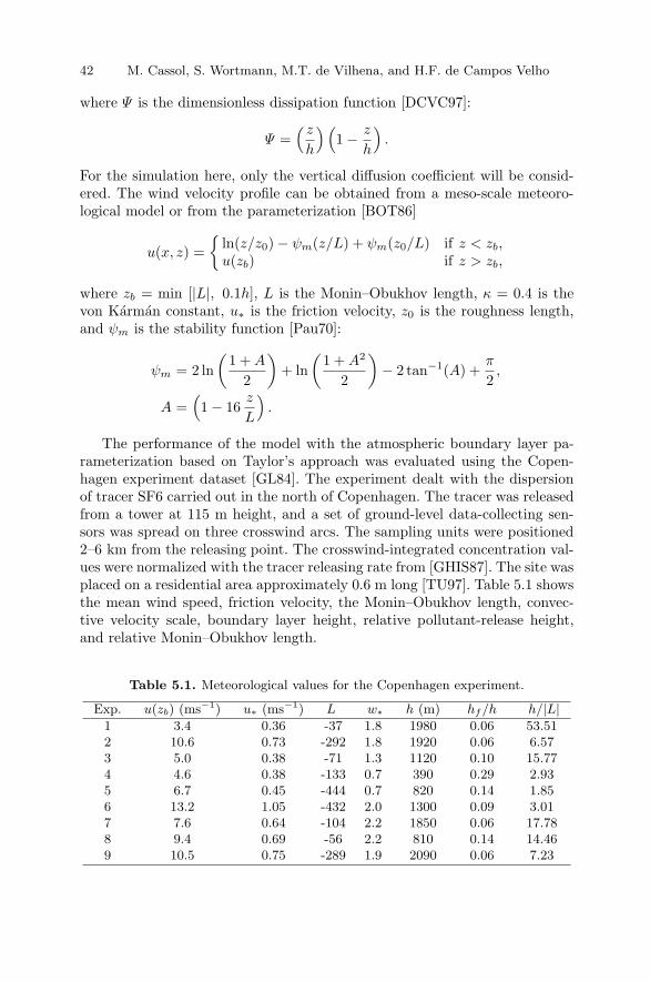
42 M. Cassol, S. Wortmann, M.T. de Vilhena, and H.F. de Campos Velho
where Ψ is the dimensionless dissipation function [DCVC97]:
Ψ =( zh
)(1 − z
h
).
For the simulation here, only the vertical diffusion coefficient will be consid-ered. The wind velocity profile can be obtained from a meso-scale meteoro-logical model or from the parameterization [BOT86]
u(x, z) =
ln(z/z0) − ψm(z/L) + ψm(z0/L) if z < zb,u(zb) if z > zb,
where zb = min [|L|, 0.1h], L is the Monin–Obukhov length, κ = 0.4 is thevon Karman constant, u∗ is the friction velocity, z0 is the roughness length,and ψm is the stability function [Pau70]:
ψm = 2 ln
(1 +A
2
)+ ln
(1 +A2
2
)− 2 tan−1(A) +
π
2,
A =(1 − 16
z
L
).
The performance of the model with the atmospheric boundary layer pa-rameterization based on Taylor’s approach was evaluated using the Copen-hagen experiment dataset [GL84]. The experiment dealt with the dispersionof tracer SF6 carried out in the north of Copenhagen. The tracer was releasedfrom a tower at 115 m height, and a set of ground-level data-collecting sen-sors was spread on three crosswind arcs. The sampling units were positioned2–6 km from the releasing point. The crosswind-integrated concentration val-ues were normalized with the tracer releasing rate from [GHIS87]. The site wasplaced on a residential area approximately 0.6 m long [TU97]. Table 5.1 showsthe mean wind speed, friction velocity, the Monin–Obukhov length, convec-tive velocity scale, boundary layer height, relative pollutant-release height,and relative Monin–Obukhov length.
Table 5.1. Meteorological values for the Copenhagen experiment.
Exp. u(zb) (ms−1) u∗ (ms−1) L w∗ h (m) hf/h h/|L|
1 3.4 0.36 -37 1.8 1980 0.06 53.512 10.6 0.73 -292 1.8 1920 0.06 6.573 5.0 0.38 -71 1.3 1120 0.10 15.774 4.6 0.38 -133 0.7 390 0.29 2.935 6.7 0.45 -444 0.7 820 0.14 1.856 13.2 1.05 -432 2.0 1300 0.09 3.017 7.6 0.64 -104 2.2 1850 0.06 17.788 9.4 0.69 -56 2.2 810 0.14 14.469 10.5 0.75 -289 1.9 2090 0.06 7.23
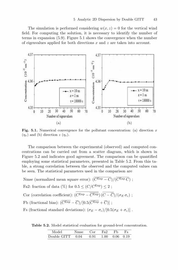
5 Analytic 2D Dispersion by Double GITT 43
The simulation is performed considering w(x, z) = 0 for the vertical windfield. For computing the solution, it is necessary to identify the number ofterms in expansion (5.9). Figure 5.1 shows the convergence when the numberof eigenvalues applied for both directions x and z are taken into account.
(a) (b)
Fig. 5.1. Numerical convergence for the pollutant concentration: (a) direction x(ηx) and (b) direction z (ηz).
The comparison between the experimental (observed) and computed con-centrations can be carried out from a scatter diagram, which is shown inFigure 5.2 and indicates good agreement. The comparison can be quantifiedemploying some statistical parameters, presented in Table 5.2. From this ta-ble, a strong correlation between the observed and the computed values canbe seen. The statistical parameters used in the comparison are
Nmse (normalized mean square error): (CExp − C)/(CExp C) ;
Fa2: fraction of data (%) for 0.5 ≤ (C/CExp) ≤ 2 ;
Cor (correlation coefficient): (CExp − CExp) (C − C)/(σE σc) ;
Fb (fractional bias): (CExp − C)/[0.5(CExp + C)] ;
Fs (fractional standard deviations): (σE − σc)/[0.5(σE + σc)] .
Table 5.2. Model statistical evaluation for ground-level concentration.
Model Nmse Cor Fa2 Fb Fs
Double GITT 0.04 0.91 1.00 0.06 0.19

44 M. Cassol, S. Wortmann, M.T. de Vilhena, and H.F. de Campos Velho
Fig. 5.2. Scatter diagram for crosswind ground-level integrated concentration: ob-served × computed (lines indicate a factor of two).
A fictitious example can be simulated, where the vertical component ofthe wind is given by
w(x, z) = wa cos(wb x);
here wb = 2π/3000 and wa ranges from 0 to 4. Figure 5.3 displays the iso-surface for the calculated concentration for two wa values, where the influenceof the vertical wind field can clearly be noted.
(a) (b)
Fig. 5.3. Iso-concentration lines for (a) wa = 0 and (b) wa = 4.

5 Analytic 2D Dispersion by Double GITT 45
5.6 Conclusion
The double GITT was derived and applied to the two-dimensional atmo-spheric pollutant dispersion problem. The computed solution shows goodagreement with the experimental data from the Copenhagen experiment[GHIS87], [GL84]. The statistical results indicate small values for the normal-ized mean-square error (Nmse), fractional bias (Fb), and fractional standarddeviation (Fs) (zero is the ideal value). In addition, the correlation coefficient(Cor) and factor of two (Fa2) are close to one.
It should be noted that other GITT schemes can be applied, such as stan-dard GITT [Cot93], [Cot97] or GILTT (generalized integral and Laplace trans-form technique) [WVCVS05]. However, the latter techniques make it difficultto control the numerical error in the calculated solution. Also, GILTT cannotbe applied in the case of variable coefficients. Finally, the truncated numericalerror can be controled using the double GITT.
References
[BOT86] Berkowicz, R.R., Olesen, H.R., Torp, U.: The Danish Gaussian airpollution model (OML): Description, test and sensitivity analysis inview of regulatory applications. In: De Wispeleare, C., Schiermeirier,F.A., Gillani, N.V. (eds.), Air Pollution Modeling and Its Applica-tion. Plenum (1986).
[Cas06] Cassol, M.: Analytical solution to the time dependent two-dimen-sional atmospheric pollutant dispersion by the Double GITT. Masterthesis. Universidade Federal do Rio Grande do Sul, Porto Alegre,Brazil (2006) (Portuguese).
[Cot93] Cotta, R.M.: Integral Transforms in Computational Heat and FluidFlow. CRC Press, Boca Raton, FL (1993).
[Cot97] Cotta, R.M., Mikhaylov, M.: Heat Conduction Lumped Analysis, In-tegral Transforms, Symbolic Computation. Wiley, Chichester (1997).
[DCVC97] Degrazia, G.A., Campos Velho, H.F., Carvalho, J.C., 1997. Nonlocalexchange coefficients for the convective boundary layer derived fromspectral properties. Contrib. Atm. Phys., 70, 57–64 (1997).
[DACTCV00] Degrazia, G.A., Anfossi, D., Carvalho, J.C., Tirabassi, T., CamposVelho, H.F.: Turbulence parameterization for PBL dispersion modelsin all stability conditions. Atm. Environ., 34, 3575–3583 (2000).
[GHIS87] Gryning, S.E., Holtslag, A.A.M., Irwin, J.S., Sivertsen, B.: Applieddispersion modeling based on meteorological scaling parameters. At-mos. Environ., 21, 79–89 (1987).
[GL84] Gryning, S.E., Lyck, E.: Atmospheric dispersion from elevatedsources in an urban area: comparison between tracer experimentsand model calculations. Bull. Am. Meteorol. Soc., 23, 651–660(1984).
[Mor06] Moreira, D.M.: Modelo Euleriano semi-analıtico de dispersao turbu-lenta de contaminantes. D.Sc. Thesis, Universidade Federal do RioGrande do Sul, Porto Alegre, Brazil (1999).

46 M. Cassol, S. Wortmann, M.T. de Vilhena, and H.F. de Campos Velho
[Ozi80] Ozisik, M.N.: Heat Conduction. Wiley, New York (1980).[Pau70] Paulson, C.A.: The mathematical representation of wind speed and
temperature profiles in unstable atmospheric surface layer. J. Appl.Meteorol., 9, 857–861 (1970).
[TU97] Tirabassi, T., Rizza, U.: Boundary layer parameterization for a non-Gaussian puff model. J. Appl. Meteorol., 36, 1031-1037 (1997).
[WVM00] Wortmann, S., Vilhena, M.T., Moura, A.: Analytical solution of theone dimensional transient pollutant problem with variable eddy dif-fusivity coefficient. National Meeting on Thermal Science (ENCIT),Brazil (2000).
[WVMB05] Wortmann, S., Vilhena, M.T., Moreira, D.M., Buske, D.: A new an-alytical approach to simulate the pollutant dispersion in the PBL.Atmos. Environ., 39, 2171–2178 (2005).
[Wo03] Wortmann, S.: Semi-analytical formulation to the transformed equa-tion from GITT application on the adective-diffusive problems. D.Sc.Thesis, Universidade Federal do Rio Grande do Sul, Porto Alegre,Brazil (2003) (Portuguese).
[WVCVS05] Wortmann, S., Vilhena, M.T., Campos Velho, H.F., Segatto, C.F.:The GILTT pollutant simulation in a stable atmosphere. In: Con-standa, C., Nashed, Z., Rollins, D. (eds.), Integral Methods in Scienceand Engineering. Birkhauser-Boston (2005), pp. 300–308.

6
Transient Acoustic Radiation from a ThinSpherical Elastic Shell
D.J. Chappell, P.J. Harris, D. Henwood, and R. Chakrabarti
University of Brighton, UK; [email protected],[email protected], [email protected],[email protected]
6.1 Introduction
The work presented in this chapter is motivated by the desire to model thetransient interaction of a vibrating loudspeaker with the surrounding air. Onepossible method for solving this problem is to employ a coupled finite elementand boundary element procedure, and one such procedure is being developedas part of this work. However, before the method is used to solve the loud-speaker problem, it will be tested on the simpler problem of acoustic radiationfrom a thin spherical shell as this has an exact solution, the details of whichare given here.
Previous work has tended to concentrate on the case of plane wave scat-tering [CD98], [GY02] and to use the exact solution of Huang [HH68] for com-parison with numerical results. This solution uses the Laplace transformationand expresses the transformed values of the quantities sought as sums of Leg-endre functions multiplied by unknown coefficients. Applying this method tospherical wave radiation simplifies the problem somewhat, since here only thefirst term of these sums is required. Huang uses an inverse transformation toobtain a solution for the transient shell displacement, but a solution for thepressure is not given due to its complexity in the frequency domain. For oursimplified problem, however, a time-domain solution for both the pressure andthe velocity potential on the surface of the shell are obtained. This enablesus to check the accuracy of both the structural and the acoustic parts of thenumerical model.
In loudspeaker modeling, it is often assumed that the effect of the airpressure acting on the loudspeaker cone can be neglected. This assumptionis investigated for several different fluid and structure combinations. Resultsfrom an uncoupled numerical model will also be compared with both thecoupled and the uncoupled exact solution. This will enable us to see howmuch of the error in the model can be attributed to coupling. A time-domainBurton–Miller-type boundary element method is used for the acoustic modelas detailed in [DC06]. The structural data used as input to this is given by an

48 D.J. Chappell, P.J. Harris, D. Henwood, and R. Chakrabarti
undamped finite element method for thin shells. This is solved using explicittime integration as detailed in [DH00].
6.2 Mathematical Formulation of the Problem
Consider a thin spherical shell with mid-surface radius a, thickness h, Young’smodulus E, Poisson’s ratio ν, and density ρ. Suppose that this shell is sur-rounded by a homogeneous compressible acoustic fluid of density ρf and soundwave speed c. The shell is assumed to be radiating a small amplitude acousticwave permitting the use of linear wave theory to describe its propagation. Aspatially-constant pressure-forcing directed into the exterior field is appliedto the shell (from the interior) causing the radiation of a spherical wave. Thetotal pressure loading acting on the shell is therefore the sum of this appliedpressure and an exterior pressure loading due to the surrounding fluid. Thesignificance of omitting this second component of the pressure will be inves-tigated later in this chapter.
The equation governing the transient motion of the shell due to a spatially-constant pressure-loading may be derived from the Lagrangian equation ofmotion for the shell as in [HH68]. This is given by
d2u(t)
dt2+
2E
ρ(1 − ν)a2u(t) =
p(a, t)
hρ, (6.1)
where u(t) is the displacement of the shell in the normal direction and p(a, t)is the total pressure loading on the shell, both evaluated at time t. Note thatthe spherically symmetric pressure is given in spherical polar coordinates, soit only depends on the radial distance from the origin and time. The shell isassumed to be at rest and undisturbed at t = 0, which gives rise to the initialconditions
u(0) = (d/dt)u(0) = 0.
For later use, note that the Laplace transform of (6.1) is given by
(s2 +
2E
ρ(1 − ν)a2
)u(s) =
p(a, s)
hρ, (6.2)
where p(a, s), u(s) are the Laplace transforms of p(a, t), u(t), respectively, ands is the transformation parameter.
The applied spherical wave pressure load can be written as pf (a, t) =p0f(t), where p0 is p0 is a constant-magnitude term for the applied pressureand f(t) governs the temporal behavior of the applied pressure. The pressurein the surrounding fluid pe(r, t) at any distance r ≥ a from the origin isgoverned by the wave equation. In spherical polar coordinates with pe(r, t)assumed to be a spherical wave, this is given by
6 Transient Acoustic Radiation 49
1
r2∂
∂r
(r2∂p
∂r
e)=
1
c2∂2p
∂t2
e
. (6.3)
The initial conditions are
pe(r, 0) = (d/dt)pe(r, 0) = 0,
as before. The Laplace transform of (6.3) is
1
r2∂
∂r
(r2∂p
∂r
e)=
s2
c2p e, (6.4)
where p e is the Laplace transform of pe. Applying the Sommerfeld radiationcondition, the solution of (6.4) is simply
p e(r, s) =α
r(sinh(rs/c) − cosh(rs/c)) , (6.5)
where α is some constant to be determined from the boundary condition atthe shell–fluid interface. This enforces the continuity of normal accelerationand is given by
∂p
∂r
e
= −ρfs2u at r = a.
Applying this boundary condition to (6.5) to determine α and then substitut-ing back in for p e yields
p e(r, s) =ρfs
2a2cu (sinh(rs/c) − cosh(rs/c))
r(as+ c)(sinh(as/c) − cosh(as/c)). (6.6)
Substituting (6.6) into the transformed structural equation (6.2), noting thatp(a, t) = pf (a, t) + pe(a, t), and solving for u leads to
u(s) =p0a
2(1 − ν)(as+ c)f(s)
ρha3(1 − ν)s3 + ca2(1 − ν)(hρ+ aρf )s2 + 2Ehas+ 2Ehc, (6.7)
where f(s) is the Laplace transform of f(t). The inverse Laplace transforma-tion may be applied to (6.7) in order to obtain the transient solution u(t). It isalso possible to obtain frequency-domain expressions for the radiated pressureand velocity potential. These expressions are in a form that is easy to invertat points on the shell, i.e., at r = a, since the hyperbolic functions cancel.The pressure is obtained by simply substituting (6.7) into (6.6). The velocitypotential ϕe may be obtained from the pressure since pe = −ρf (∂/∂t)ϕe, andhence, its Laplace transform is given by ϕ e = −p e/(ρfs). We arrive at theexpression
ϕ e(a, s) =−cp0a
3(1 − ν)sf(s)
ρha3(1 − ν)s3 + ca2(1 − ν)(hρ+ aρf )s2 + 2Ehas+ 2Ehc. (6.8)

50 D.J. Chappell, P.J. Harris, D. Henwood, and R. Chakrabarti
The inverse Laplace transforms of (6.7) and (6.8) may be computed in asimilar way because they share the same cubic polynomial denominator q(s).Let us define the following common factor of these expressions:
g(s) :=p0a
2(1 − ν)
q(s).
We denote its inverse Laplace transform by g(t). Applying the convolutionand derivative theorems for Laplace transforms, we deduce that the inversetransforms are
u(t) =
(c+ a
d
dt
)f(t) ∗ g(t),
ϕe(t) = −acdf(t)
dt∗ g(t).
The calculation of g(t) follows from the Bromwich inversion formula andCauchy’s residue theorem. This yields
g(t) =∑
j
Res(g(s)est, sj),
where Res(F, x) denotes the residue of F at x and sj denotes the values of sthat are poles of g(s)est. The values sj are clearly just the roots of q(s).
The component of the pressure loading on the shell due to the exteriorfluid may be omitted by setting pe(a, t) = p e(a, s) = 0 in the structuralequations (6.1), (6.2). This has the effect of changing the coefficient of s2 inq(s) to ρhca2(1 − ν). In this case, the roots of q(s) are given by s1 = −c/a,s2 =
√2E/(a
√ρ(ν − 1)), and s3 = −s2. In the coupled case, these roots do
not have such nice expressions but may be calculated easily by computer.
6.3 Example Problems
The numerical calculations are carried out for a spherical shell with a = 0.1m and h = 0.75 mm, so the size of the problem is of similar order to theloudspeaker problem. Three different fluid–structure interactions are consid-ered. Air–steel and water–steel are examples in which the coupling would beexpected to be insignificant and significant, respectively. The third exampleconsidered is air–paper, due to its similarity to the loudspeaker cone problem.The material parameters are summarized in Table 6.1.
The forcing function f(t) is chosen to be a raised cosine, defined by f(t) =(1 − cos(2πt/t0))H(t0 − t), where t0 is the period of the raised cosine pulseand H is the Heaviside step function. The value of the constant p0 is takento be 105.
Figure 6.1 shows the results of solving both the coupled and the uncoupledsystems for the velocity potential ϕe on the surface of the shell, with each row

6 Transient Acoustic Radiation 51
Table 6.1. Material/fluid parameters.
Structure Materials ρ (kgm−3) E (Pa) ν
Steel 7800 209 × 109 0.3Paper 500 3 × 10⁹ 0.333
Exterior Fluids ρf (kgm−3) c (ms−1)
Water 1000 1500Air 1.21 342.4
showing one of the three fluid–structure combinations considered. In eachcase, two values of t0 are considered: t0 = 0.001 s in the left column andt0 = 0.0004 s in the right. The total duration of the solution in each case is4t0, and the solutions are calculated at 1024 points in this interval. The resultsshow the expected trends of the coupling being most important in the steel–water interaction and least important for steel–air. The coupling also tends tobe more significant for the smaller choice of t0, i.e., for higher frequencies. AFourier transform shows that for t0 = 0.0004, f(t) is essentially bandlimitedat 10000 Hz and for t0 = 0.001, f(t) is essentially bandlimited at 4000 Hz.The coupling is more significant at these higher forcing frequencies as thenresonance frequencies of the structure become excited and the coupling actsas a damping force on them.
The error when using an uncoupled numerical scheme to obtain the surfacevelocity potential solution is now considered. The structural data are calcu-lated using a time-domain finite-element procedure with thin shell elements.The procedure is carried out using explicit time integration and is describedin [DH00]. These data are used as input for a time-domain Burton–Millerboundary element method (BEM) to solve the acoustic part of the problem.This technique is employed because of its superior stability properties com-pared with other time-domain boundary element methods, and is detailedin [DC06]. The error is calculated with respect to both the coupled and theuncoupled exact solutions described above, and is given by
Error =1
n
n∑
i=1
√√√√∑N
j=1 |ϕe(a, tj) − ϕe(xi, tj)|2∑N
j=1 |ϕe(a, tj)|2.
Here ϕe and ϕe denote the exact and modeled values of the velocity potential,respectively, xi, i = 1, . . . , n, denotes the n boundary elements, and tj , j =1, . . . , N, denotes the jth time at which the solution is computed. The BEMis a time-marching method with time-step ∆t and so tj = (j − 1)∆t. Thiserror is therefore an L2-relative error averaged over the n boundary elements.Additional details of the numerical methods are omitted for brevity.
Figure 6.2 shows how the error in the uncoupled numerical method com-pared with both the coupled and the uncoupled exact solutions varies with

52 D.J. Chappell, P.J. Harris, D. Henwood, and R. Chakrabarti
Fig. 6.1. Coupled vs. uncoupled surface velocity potential solution.
the number n of boundary elements. The cases considered are the same as be-fore with the exception of the steel–water interaction, where the error for thecoupled exact solution would clearly be very large. The steel–air interactionresults are shown in the top row, and the paper–air results are in the secondrow. The left column shows the errors for the lower frequency case, t0 = 0.001,and the right column shows the higher frequency case, t0 = 0.0004, as before.The solutions were computed at 320 time-points in the interval [0, 4t0], sincethis gave a time-step for the BEM whose Nyquist frequency is ten times the

6 Transient Acoustic Radiation 53
essential band limit of f . Previous work has indicated this solution to be agood choice for accurate results [DC06].
Fig. 6.2. Error in uncoupled modeled solution compared against both coupled anduncoupled exact solutions.
The results show that the error decreases as n is increased and is greaterfor the higher-frequency case, as expected. The coupling is more significant forthe paper–air interaction and as n is increased. The significance of the couplingcan be viewed in two ways. First, it can be regarded as the percentage of theerror with the coupled solution that arises due to the numerical method beinguncoupled, which may be calculated using (Ec −Eu)/Ec × 100, where Ec andEu are the errors with the coupled and uncoupled exact solutions, respectively.This shows that for the steel–air case, the coupling becomes most significantfor the higher-frequency forcing when n = 32, where the coupling accounts forjust 2.15% of the total error. In contrast, for the paper–air interaction withn = 34, the coupling accounts for 80.5% of the total error when t0 = 0.001 and

54 D.J. Chappell, P.J. Harris, D. Henwood, and R. Chakrabarti
for 76.9% when t0 = 0.0004. Clearly, the coupling is vastly more significantin the paper–air interaction. Alternatively, the magnitude of the error withthe coupled solution may be considered on its own and the coupling may bedeemed insignificant if this error is reasonably small. This error is greatestin the high-frequency paper–air case, where for n = 32 the error is 0.126,or 12.6%. This may even be regarded as sufficiently accurate in loudspeakermodeling, where errors due to lack of measurement precision and inaccuratelyestimated material parameters generally dominate.
6.4 Conclusion
An exact solution for modeling transient acoustic radiation from a thin spheri-cal elastic shell has been presented. The effect of omitting the pressure exertedby the exterior fluid back on the shell (or coupling) from the solution has beeninvestigated for several different fluid–structure interactions. A raised cosine-type forcing of varying pulse width has been used. For shorter pulses and thushigher frequencies, the coupling has been shown to have a damping effect onthe resonant behavior of the shell. The coupling is therefore more significant inthis case than for wider pulses, which do not excite resonances of the shell tothe same degree. The effect of the coupling has also been observed to be mostpronounced in the steel–water interaction, where the fluid is relatively dense.For lighter fluids like air, the coupling is less significant, although this mayvary depending on the material properties of the shell. A comparison with anuncoupled numerical solution showed that the percentage of the error causedby not coupling the numerical method was far greater for the paper–air in-teraction than the steel–air interaction. However, reasonably accurate resultscould be obtained in both cases with suitable refinement of the numericalmodel.
Acknowledgement. The partial funding of this work by B&W Group Limited, Steyn-ing, West Sussex, UK, is gratefully acknowledged.
References
[HH68] Huang, H.: Transient interaction of plane acoustic waves with a sphericalelastic shell. J. Acoust. Soc. Amer., 45, 661–670 (1968).
[CD98] Dyka, C.T., Ingel, R.P.: Transient fluid–structure interaction in naval ap-plications. Engrg. Anal. Boundary Elements, 21, 245–251 (1998).
[DH00] Henwood, D., Moore, J., Geaves, G., Fryer, P.: Towards the transient mod-elling of loudspeaker diaphragm/surround boundaries. AES 108th Con-vention Preprints, 5166, (2000).
[GY02] Yu, G.Y., Lie, S.T., Fan, S.C.: Stable BEM/FEM procedure for dynamicfluid–structure interactions. J. Engrg. Mech., 128, 909–915 (2002).
[DC06] Chappell, D.J., Harris, P.J., Henwood, D., Chakrabarti, R.: A stableboundary element method for modeling transient acoustic radiation. J.Acoust. Soc. Amer., 120, 74–80 (2006).

7
The Eigenfrequencies and Mode Shapes ofDrilling Masts
S. Chergui
Entreprise Nationale des Travaux aux Puits, Hassi-Messaoud, Algeria;[email protected]
7.1 Introduction
A drilling mast is a thin, metallic spatial structure that generally consists oftubular or straight-shaped uniform bars rigidly assembled together at theirends, called elastic nodes. It can be of one of two types, A or U (see Figure 7.1).The mast, erected above the opening of a well, enables the vertical motionof the traveling block and has the following major functional roles: (i) tosustain—by means of the hoisting system (drawworks, drilling line, crownblock, traveling block, hook, and swivel)—the drill string, the casing string,and the tubing string, and to make possible their up-and-down operation;(ii) to store the drill pipes, drill collars, and tubing; and (iii) to facilitate thedrilling and tool-running procedures. Consequently, the drilling mast is of vitalimportance to a drilling rig. When in use, masts undergo strong vibrations,caused by the motion of the tubular string, of the driving equipment of thedrilling machines, and of the floating platforms (in an offshore setup), andby winds. Excessive vibrations of these structures can generate undesirableeffects and decrease significantly the lifetime of their parts. Such effects mayinclude the wear of pins and their housing or the fatigue and buckling ofcertain bars. High-performance and economical design, and the rational useof drilling masts, especially of those intended for very deep and ultra-deepwells, require a rigorous theoretical and experimental investigation of theirdynamical behavior. The first and most important step in this research is thedetermination of the eigenfrequencies and of the mode shapes of vibration.
7.2 Proposed Dynamical Model
In practical engineering, the mast strength is calculated by means of simpleequivalent patterns of the structures, which allow us to determine the stressesand to compute the dimensions and principal elements of the mast. This typeof calculation gives satisfactory results. When performing it, we have to deal

56 S. Chergui
Fig. 7.1. Drilling masts of types A and U.
with the complex structural composition of the masts and of the acting loadmode. We must keep in mind that we should use a minimum amount of steelto obtain a mast with a high technical and economic performance. In addition,because of the importance of drilling masts in drilling rigs, the masts mustbe designed using an adequate dynamical model and a rigorous method ofcalculation based on the sophisticated software packages currently available.
The proposed dynamical model for a drilling mast is obtained [Ch90] byapplying the concentrated masses method. This method makes use of the factthat the distributed masses of the structure bars are concentrated at theirjunctions, called nodes; therefore, the total concentrated mass at each nodeis equal to the sum of the nodal contribution of each bar joining at the cor-responding node. Those masses are assumed to be connected by a masslesslink. Figure 7.2 shows the dynamical models for masts of type A and U. Usingthis model, we can regard a mast as a discrete system with a finite number ofdegrees of freedom and with the same geometric configuration as the real struc-ture. The number of degrees of freedom is equal to the number of independentparameters specifying the translations and rotations of the nodes. Choosingthe node parameters as unknowns, we obtain the displacement method. Thismethod is the most recommended for the static and dynamic computationof bar-assembled structures; hence, it can also be applied to drilling masts.
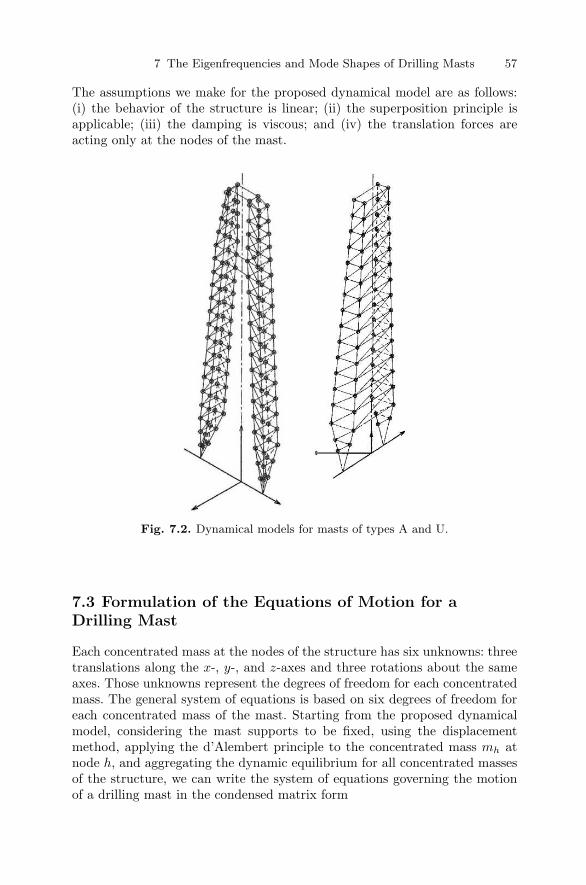
7 The Eigenfrequencies and Mode Shapes of Drilling Masts 57
The assumptions we make for the proposed dynamical model are as follows:(i) the behavior of the structure is linear; (ii) the superposition principle isapplicable; (iii) the damping is viscous; and (iv) the translation forces areacting only at the nodes of the mast.
Fig. 7.2. Dynamical models for masts of types A and U.
7.3 Formulation of the Equations of Motion for aDrilling Mast
Each concentrated mass at the nodes of the structure has six unknowns: threetranslations along the x-, y-, and z-axes and three rotations about the sameaxes. Those unknowns represent the degrees of freedom for each concentratedmass. The general system of equations is based on six degrees of freedom foreach concentrated mass of the mast. Starting from the proposed dynamicalmodel, considering the mast supports to be fixed, using the displacementmethod, applying the d’Alembert principle to the concentrated mass mh atnode h, and aggregating the dynamic equilibrium for all concentrated massesof the structure, we can write the system of equations governing the motionof a drilling mast in the condensed matrix form

58 S. Chergui
[M ]η(t) + [B]η(t) + [R]η(t) = F (t),
where [M ] is the diagonal square matrix of inertia of order N , [B] is thesymmetric damping matrix of order N , [R] is the symmetric stiffness matrixof order N , η(t) is the displacement vector of order N , F (t) is the vectorof order N of the excitation forces acting on the concentrated masses, N isthe total number of degrees of freedom (translations and rotations) of thedynamical model, and t is the time variable.
This latter system of equations with six unknowns for each node is iden-tical to the well-known classical set of differential equations of second orderdescribing the damped forced vibrations of a linear discrete spatial structure(see [Me67], [Wa76], and [Cl75]). Analytically, this system is decomposed intoa set of N second-order differential equations. In the case of drilling masts,where the dimensions of the concentrated masses are lowered, their rotatoryinertia may be neglected and the number of unknowns at each node reducesto only three (three translations) instead of six. Hence, the general system ofequations of motion for drilling masts becomes
[M∆]∆(t) + [B∆]∆(t) + [R∆]∆t = F∆(t),
where [M∆], [B∆], and [R∆] are the matrices M , B, and R of concentratedmasses of order N∆ corresponding to translations only, ∆(t) is the dis-placement vector of order N∆ of the concentrated masses with respect totranslations, F∆(t) is the vector of order N∆ of the excitation forces actingon the concentrated masses along the x-, y-, and z-axes, and N∆ is the totalnumber of degrees of freedom (translations only) of the dynamical model.
This system represents the equations of motion for the drilling mast whenthe rotatory inertia of the concentrated masses is neglected; hence, it containsonly half of the unknowns of the general system of equations of motion basedon six unknowns for each node. Without any adverse effect on the results,this represents an important reduction of computation time for the dynamicalanalysis of a drilling mast. Analytically, this system may be decomposed intoa set of N∆ second-order differential equations.
7.4 The Eigenfrequencies and Mode Shapes ofVibrations
It is obvious that the equations of free vibrations of a drilling mast whendamping is taken into account are
[M∆]∆(t) + [B∆]∆(t) + [R∆]∆(t) = 0,
where 0 is the zero vector of order N∆. As the influence of damping onthe eigenfrequencies of the vibrations of the structure is negligible, we may

7 The Eigenfrequencies and Mode Shapes of Drilling Masts 59
discard the damping effect. Therefore, the eigenfrequencies of a drilling mastcan be determined from the set of differential equations for free oscillations
[M∆]∆(t) + [R∆]∆t = 0.
This means that the eigenfrequency equation is
∣∣[R∆] − p2[M∆]∣∣ = 0,
that is, an algebraic equation of order N∆ in p2. The eigenfrequencies pα
of order α and their corresponding mode shapes of vibration can also bedetermined. Knowing the mode shapes of vibration, we can obtain the freevibrations of the drilling mast as a linear combination of the mode shapes,that is,
∆free vib.(t)
= [V1 cos (p1t− θ1) . . . Vα cos (pαt− θα) . . .] [C1 . . . Cα . . . CN∆]T,
where∆free vib.(t)
is the column vector of the elongations of the discrete
masses in free vibration, Cα, θα are the constants of the eigenmodes, whichcan be identified as the amplitudes and phase angles of order α, and Vα isthe column matrix of mode shapes of order α.
7.5 Numerical Application
Using the algorithm proposed in this chapter and the program version SAP05, we have obtained the eigenfrequencies and mode shapes of vibration of aworking drilling mast for a drilling rig of type A designed for very deep wellsof up to 7000 m, with drill pipes of 4.5′′. The mast legs have rectangular crosssections and consist of 539 tubular bars and 194 moving nodes. The distributedmasses of the bars of the structure are replaced by concentrated masses at thenodes. Neglecting the rotatory inertia of the concentrated masses, we are leftto consider a dynamical model with 194×3 degrees of freedom. The dynamicalcomputation of the proposed model by means of the programme SAP 05 needsthe following data input: (i) the numerical labeling of the nodes and bars ofthe mast starting from the base to the top; (ii) the coordinates of the nodes inthe Cartesian coordinate system of the dynamical model; (iii) the geometriccharacteristics: the cross-sectional area and the axial moments of inertia ofeach bar of the mast; and (iv) the physical characteristics E (longitudinalmodulus of elasticity), µ (Poisson ratio), and ρ (density) of the bars.
With this input in SAP 05, the computer calculates the stiffness matrixfor each bar of the mast, which is required for the dynamical computation ofthe eigenfrequencies. In Table 7.1 we present only the values of the first sixeigenfrequencies of the mast.

60 S. Chergui
Table 7.1. The first six eigenfrequencies of a working mast.
Eigenfrequency p1 p2 p3 p4 p5 p6
[rad./s] 4.35 7.72 19.00 21.88 24.79 28.45
7.6 Interpretation of the Results
The analysis of the results obtained in this study allows us to draw severalconclusions.
(i) The eigenfrequencies are relatively low and close to each other. Thiscan be explained by the flexibility of the drilling masts. Also, certain eigen-frequencies are included in the domain of angular velocities of the drill string(in the case of rotatory drilling) during drilling operations. This last charac-teristic is often noticed in the field during drilling for almost all masts, sowe should change the rotational speed of the drill string in order to avoidexcessive vibrations of the masts.
(ii) The mode shapes of the vibrations are normalized.
(iii) The first four mode shapes, exhibited only by the support leg of themast and the upper cross section on which the crown block is set, representbending in the (y, z)-plane, traction in the (x, y)-plane, and torsion about thevertical y-axis.
(iv) Taking into account the energy needed for the excitation of the mast,we assessed that during the tripping operations, which can put the mast out-side the elastic equilibrium position, the dynamical deformation of the mastis due to the bending generated by the contribution of the first two oscillationmodes.
7.7 Conclusions
(i) The dynamical model adopted here and the corresponding algorithm de-signed in this chapter can be applied to evaluate the eigenfrequencies of anytype of mast.
(ii) It is evident that knowing the eigenfrequencies allows us to avoid theresonance phenomenon in the drilling mast elements and other surface equip-ment of a drilling rig, by changing the rotational speeds of the drill string.But if the drilling program of a well requires angular velocities of the drillstring equal to certain eigenfrequencies of the drilling mast, then we mustdrill at that speed to reduce the control timing of the drilling mast and ofother surface equipment.
(iii) Furthermore, it is easy to see that to determine the eigenfrequenciesand mode shapes of vibration of a mast in matrix-calculation theory means

7 The Eigenfrequencies and Mode Shapes of Drilling Masts 61
to establish the eigenvalues and eigenvectors of the dynamical stiffness matrixcorresponding to the degrees of freedom of the translations of the mast.
References
[Ch90] Chergui, S.: Research concerning the dynamics of a drilling system and mastvibrations. PhD Thesis, Petroleum and Gas Institute, Ploesti, Romania(1990).
[Cl75] Clough, R.W., Penzien, J.: Dynamics of Structures. Vol. 1. FundamentalPrinciples. McGraw-Hill, New York (1975).
[Me67] Meirovitch, L.: Analytical Methods in Vibrations. Macmillan, New York(1967).
[Wa76] Warburton, B.G.: The Dynamical Behavior of Structures. Pergamon Press,London (1976).


8
Layer Potentials in Dynamic Bending ofThermoelastic Plates
I. Chudinovich and C. Constanda
University of Tulsa, OK, USA; [email protected],[email protected]
8.1 Introduction
The static transverse shear deformation model of elastic plates (see, for ex-ample, [Co90], [ChCo00], and [ChCo05]) was generalized to the thermoelasticcase in [ScTa93] and [ScTa95]. In this chapter, we solve the time-dependentbending of a thin elastic plate subject to external forces, moments, inter-nal heat sources, homogeneous initial conditions, and Dirichlet or Neumannboundary conditions by reducing the governing equations to time-dependentboundary integral equations with the help of layer potentials and showing theunique solvability of these equations in a variational setting.
A full analysis when thermal effects are not present can be found in[ChCo05] and in [ChCo99], [ChCo00a], [ChCo02], and [ChCo03]. The bound-ary integral equations arising in the fundamental problems of three-dimension-al thermoelasticity [KGBB78] were studied in [ChDu00].
In what follows, we consider a plate with zero initial data. This implies norestriction on generality since homogeneous conditions can easily be achievedby means of an “area” and some “initial” thermoelastic plate potentials (see[ChCo04] and [ChCo06]).
8.2 Preliminaries
We consider a thin elastic plate of thickness h0 = const > 0, which occupiesa region S × [−h0/2, h0/2] in R
3, where S is a domain in R2 with bound-
ary ∂S. The displacement vector at a point x′ in this region at t ≥ 0 isv(x′, t) = (v1(x
′, t), v2(x′, t), v3(x
′, t))T , where the superscript T denotes ma-trix transposition, and the temperature is θ(x′, t). We write x′ = (x, x3),x = (x1, x2) ∈ S. We assume [Co90] that
v(x′, t) = (x3u1(x, t), x3u2(x, t), u3(x, t))T .
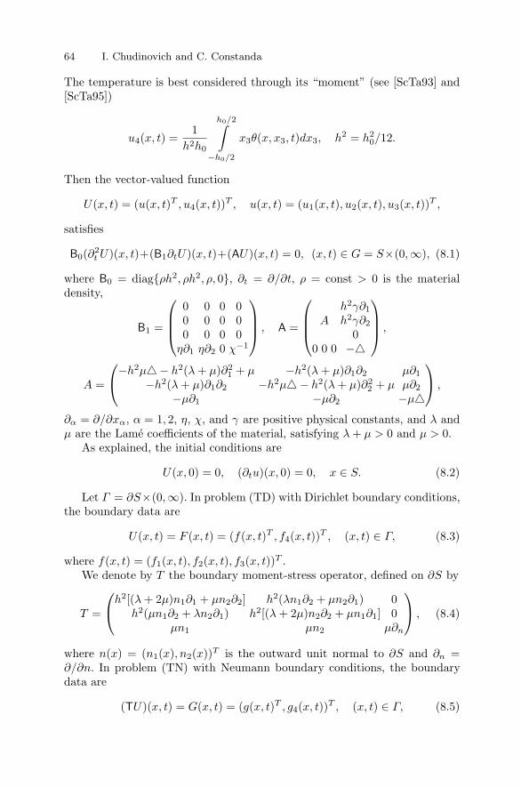
64 I. Chudinovich and C. Constanda
The temperature is best considered through its “moment” (see [ScTa93] and[ScTa95])
u4(x, t) =1
h2h0
h0/2∫
−h0/2
x3θ(x, x3, t)dx3, h2 = h20/12.
Then the vector-valued function
U(x, t) = (u(x, t)T , u4(x, t))T , u(x, t) = (u1(x, t), u2(x, t), u3(x, t))
T ,
satisfies
B0(∂2tU)(x, t)+(B1∂tU)(x, t)+(AU)(x, t) = 0, (x, t) ∈ G = S×(0,∞), (8.1)
where B0 = diagρh2, ρh2, ρ, 0, ∂t = ∂/∂t, ρ = const > 0 is the materialdensity,
B1 =
⎛⎜⎜⎝
0 0 0 00 0 0 00 0 0 0η∂1 η∂2 0 χ−1
⎞⎟⎟⎠ , A =
⎛⎜⎜⎝
Ah2γ∂1
h2γ∂2
00 0 0 −
⎞⎟⎟⎠ ,
A =
⎛⎝
−h2µ − h2(λ+ µ)∂21 + µ −h2(λ+ µ)∂1∂2 µ∂1
−h2(λ+ µ)∂1∂2 −h2µ − h2(λ+ µ)∂22 + µ µ∂2
−µ∂1 −µ∂2 −µ
⎞⎠ ,
∂α = ∂/∂xα, α = 1, 2, η, χ, and γ are positive physical constants, and λ andµ are the Lame coefficients of the material, satisfying λ+ µ > 0 and µ > 0.
As explained, the initial conditions are
U(x, 0) = 0, (∂tu)(x, 0) = 0, x ∈ S. (8.2)
Let Γ = ∂S×(0,∞). In problem (TD) with Dirichlet boundary conditions,the boundary data are
U(x, t) = F (x, t) = (f(x, t)T , f4(x, t))T , (x, t) ∈ Γ, (8.3)
where f(x, t) = (f1(x, t), f2(x, t), f3(x, t))T .
We denote by T the boundary moment-stress operator, defined on ∂S by
T =
⎛⎝h2[(λ+ 2µ)n1∂1 + µn2∂2] h2(λn1∂2 + µn2∂1) 0
h2(µn1∂2 + λn2∂1) h2[(λ+ 2µ)n2∂2 + µn1∂1] 0µn1 µn2 µ∂n
⎞⎠ , (8.4)
where n(x) = (n1(x), n2(x))T is the outward unit normal to ∂S and ∂n =∂/∂n. In problem (TN) with Neumann boundary conditions, the boundarydata are
(TU)(x, t) = G(x, t) = (g(x, t)T , g4(x, t))T , (x, t) ∈ Γ, (8.5)

8 Dynamic Bending of Thermoelastic Plates 65
where g(x, t) = (g1(x, t), g2(x, t), g3(x, t))T and
(TU)(x, t) =
((Tu)(x, t) − h2γn(x)u4(x, t)
∂nu4(x, t)
)=
((TeU)(x, t)(TθU)(x, t)
). (8.6)
In (8.6) and below, n(x) also stands for the vector (n1(x), n2(x), 0)T .Let S+ and S− be the interior and exterior domains bounded by ∂S, and
let G± = S± × (0,∞). The classical interior and exterior problems (TD±)consist in finding U ∈ C2(G±) ∩ C1(G±) that satisfy (8.1) in G±, (8.2) inS±, and (8.3). The classical interior and exterior problems (TN±) consist infinding U ∈ C2(G±)∩C1(G±) that satisfy (8.1) in G±, (8.2) in S±, and (8.5),which we write in the form
(TU)±(x, t) = (T±U)(x, t) = G(x, t), (x, t) ∈ Γ.
The superscripts ± denote the limiting values of the corresponding functionsas (x, t) → Γ from inside G±.
To solve the above initial-boundary value problems, we start by consideringtheir Laplace-transformed (with respect to t) versions (TD±
p ) and (TN±p ).
8.3 The Laplace-Transformed Boundary Value Problems
Let L and L−1 be the direct and inverse Laplace transformations, and letU(x, p) be the Laplace transform of U(x, t), where p is the transformationparameter.
The transformed problems (TD±p ) consist in finding U(x, p) ∈ C2(S±) ∩
C1(S±) such that
p2B0U(x, p) + p (B1U)(x, p) + (AU)(x, p) = 0, x ∈ S±,
U±(x, p) = F (x, p), x ∈ ∂S.
In problems (TN±p ), we search for U(x, p) ∈ C2(S±) ∩ C1(S±) such that
p2B0U(x, p) + p (B1U)(x, p) + (AU)(x, p) = 0, x ∈ S±,
(T±U)(x, p) = G(x, p), x ∈ ∂S.
Our analysis requires the introduction of certain function spaces, whichwe list below. Let m ∈ R and p ∈ C.
Hm(R2) : the standard Sobolev space of all v4(x), x ∈ R2, with norm
‖v4‖m =
∫
R2
(1 + |ξ|2)m|v4(ξ)|2 dξ1/2
,
where v4(ξ) is the Fourier transform of v4(x).

66 I. Chudinovich and C. Constanda
Hm,p(R2) : the space of all v(x) = (v1(x), v2(x), v3(x))T in the underlying set
of[Hm(R2)
]3, with norm
‖v‖m,p =
∫
R2
(1 + |ξ|2 + |p|2)m|v(ξ)|2 dξ1/2
.
Hm,p(R2) = Hm,p(R
2) ×Hm(R2), with norm ‖|V ‖|m,p = ‖v‖m,p + ‖v4‖m.
Hm(S±), Hm,p(S±): the spaces of the restrictions to S± of all v4 ∈ Hm(R2),
v ∈ Hm,p(R2), respectively, with norms
‖u4‖m;S± = infv4∈Hm(R2):v4|S± =u4
‖v4‖m,
‖u‖m,p;S± = infv∈Hm,p(R2):v|S± =u
‖v‖m,p.
Hm,p(S±) = Hm,p(S
±) ×Hm(S±), with norm
‖|U‖|m,p;S± = ‖u‖m,p;S± + ‖u4‖m;S± .
Hm(R2) = Hm,0(R2) =
[Hm(R2)
]3, Hm(S±) = Hm,0(S
±) = [Hm(S±)]3.
Hm(R2) = Hm(R2) ×Hm(R2) =[Hm(R2)
]4.
Hm(S±) = Hm(S±) ×Hm(S±) = [Hm(S±)]4.
The norms on[Hm(R2)
]nand [Hm(S±)]
nare denoted by the same sym-
bols ‖ · ‖m and ‖ · ‖m;S± for all n = 1, 2, . . . .
Hm(S±), Hm,p(S±), Hm,p(S
±) = Hm,p(S±) × Hm(S±) : the subspaces of
Hm(R2), Hm,p(R2), Hm,p(R
2) of all v4 ∈ Hm(R2), v ∈ Hm,p(R2), V ∈
Hm,p(R2) with supp v4 ⊂ S±, supp v ⊂ S±, supp V ⊂ S±.
H−m(S±), H−m,p(S±), H−m,p(S
±) : the duals of Hm(S±), Hm,p(S±),
Hm,p(S±) with respect to the dualities generated by the inner products in
L2(S±),[L2(S±)
]3,[L2(S±)
]4. In what follows, (· , ·)0;S± is the inner prod-
uct in[L2(S±)
]nfor all n = 1, 2, . . . .
We assume that the boundary contour ∂S is a simple, closed, C2-curve.
H1/2(∂S), H1/2,p(∂S) : the spaces of the traces on ∂S of all u4 ∈ H1(S±),
u ∈ H1,p(S±), equipped with the norms
‖ϕ4‖1/2;∂S = infu4∈H1(S+):u4|∂S =ϕ4
‖u4‖1,S+ ,
‖ϕ‖1/2,p;∂S = infu∈H1,p(S+):u|∂S =ϕ
‖u‖1,p;S± .
H1/2,p(∂S) = H1/2,p(∂S) ×H1/2(∂S), with norm

8 Dynamic Bending of Thermoelastic Plates 67
‖|F‖|1/2,p;∂S = ‖ϕ‖1/2,p;∂S + ‖ϕ4‖1/2;∂S .
The continuous (uniformly with respect to p ∈ C) trace operators fromH1(S
±) to H1/2(∂S), from H1,p(S±) to H1/2,p(∂S), and from H1,p(S
±) toH1/2,p(∂S), are denoted by the same symbols γ±.
H−1/2(∂S), H−1/2,p(∂S), H−1/2,p(∂S) : the duals of H1/2(∂S), H1/2,p(∂S),H1/2,p(∂S) with respect to the dualities generated by the inner products
in L2(∂S),[L2(∂S)
]3,[L2(∂S)
]4. In what follows, (· , ·)0;∂S is the inner
product in[L2(∂S)
]nfor all n = 1, 2, . . . . The norms of g4 ∈ H−1/2(∂S),
g ∈ H−1/2,p(∂S), G = (gT , g4)T ∈ H−1/2,p(∂S) are denoted by ‖g4‖−1/2;∂S ,
‖g‖−1/2,p;∂S , ‖|G‖|−1/2,p;∂S = ‖g‖−1/2,p;∂S + ‖g4‖−1/2;∂S .
H±1/2(∂S) = H±1/2,0(∂S) =[H±1/2(∂S)
]3.
H±1/2(∂S) = H±1/2(∂S) ×H±1/2(∂S) =[H±1/2(∂S)
]4.
The norms on[H±1/2(∂S)
]nare denoted by the same symbols ‖ · ‖±1/2;∂S
for all n = 1, 2, . . . .Let U = (uT , u4)
T , W = (wT , w4)T ∈ H1,p(S
±). We write
Υ±,p(U , W ) = a±(u, w) + (∇u4,∇w4)0;∂S± + p2(B1/20 u, B
1/20 w)0;S±
+ χ−1p (u4, w4)0;S± − h2γ(u4,div w)0;S± + ηp (div u, w4)0,S± ,
where B0 = diag ρh2, ρh2, ρ, a±(u, w) = 2∫
S±
E(u, w) dx, and E is the
sesquilinear form of the internal static energy density [ChCo00].U ∈ H1,p(S
±) is called a weak (variational) solution of (TD±p ) if
Υ±,p(U , W ) = 0 ∀W ∈[H1(S
±)]4, γ±U = F .
Let G ∈ H−1/2,p(∂S). For any W ∈ H1/2,p(∂S), we write
L(W ) = (G, W )0;∂S = (g, w)0;∂S + (g4, w4)0;∂S .
The variational problems (TN±p ) consist in finding U ∈ H1,p(S
±) such that
Υ±,p(U , W ) = ±L(W ) ∀W ∈[H1(S
±)]4.
Let Cκ = p = σ + iζ ∈ C : σ > κ. Below, we denote by c all positiveconstants occurring in estimates, which are independent of the functions inthose estimates and of p ∈ Cκ but may depend on κ. Two following assertionswere proved in [ChCo05a].
Theorem 1. For all F (x, p) ∈ H1/2,p(∂S), p ∈ Cκ, κ > 0, problems (TD±p )
have unique solutions U(x, p) ∈ H1,p(S±). If the mapping F : Cκ → H1/2(∂S)
is holomorphic, then so are U : Cκ → H1(S±).
Theorem 2. For all G(x, p) ∈ H−1/2,p(∂S), p ∈ Cκ, κ > 0, problems
(TN±p ) have unique solutions U(x, p) ∈ H1,p(S
±). If the mapping G : Cκ →H−1/2(∂S) is holomorphic, then so are U : Cκ → H1(S
±).

68 I. Chudinovich and C. Constanda
8.4 Layer Potentials for the Laplace-TransformedProblems
Let D(x, t) be a matrix of fundamental solutions for (8.1), which van-ishes for t < 0, and let A(x, t) = (α(x, t)T , α4(x, t))
T , where α(x, t) =(α1(x, t), α2(x, t), α3(x, t))
T , be a smooth function with compact support in∂S × R, which is equal to zero for t < 0. We define the single-layer thermoe-lastic plate potential (VA)(x, t) with density A(x, t) by
(VA)(x, t) =
∫
Γ
D(x− y, t− τ)A(y, τ) dsy dτ, (x, t) ∈ R3.
Its Laplace transform is
(VpA)(x, p) =
∫
∂S
D(x− y, p)A(y, p) dsy, x ∈ R2, p ∈ C0.
Let Ck,α(S±) and Ck,α(∂S) be the spaces of functions whose derivativesup to order k are Holder continuous with index α ∈ (0, 1] in S± and on ∂S,respectively. To simplify the notation, we use the symbols C, Ck,α, and Cm
for the appropriate spaces of both scalar and vector-valued functions.(i) If A ∈ C(∂S), then (VpA)(x, p) exists for any x ∈ R
2, the restrictions
of (VpA)(x, p) to S± belong to C∞(S±), and
p2B0(VpA)(x, p) + p (B1(VpA))(x, p) + (A(VpA))(x, p) = 0, x ∈ S±.
Also, VpA ∈ C0,α(R2) for any α ∈ (0, 1). Thus, the limiting values of
(VpA)(x, p), as x → ∂S from inside S±, coincide and we write
(VpA)+(x, p) = (VpA)−(x, p) = (VpA)(x, p), x ∈ ∂S.
Let Vp be the boundary operator defined by A(x) → (VpA)(x, p), x ∈ ∂S,which maps C(∂S) continuously to C0,α(∂S) for any α ∈ (0, 1).
(ii) If A ∈ C0,α(∂S), α ∈ (0, 1], then VpA ∈ C1,β(S±), with β = α forα ∈ (0, 1) and any β ∈ (0, 1) for α = 1.
Let x0 ∈ ∂S, and consider the vector-valued function (T(VpA))(x, p),where x ∈ S+ or x ∈ S− and T is defined by (8.4) and (8.6) with n = n(x0).Then
(T(VpA))(x, p) =
∫
∂S
TD(x− y, p)A(y, p) dsy. (8.7)
By (8.7) and the properties of single-layer potentials in static problems[Co90], we find that there exist limiting values (T(VpA))±(x0, p), x0 ∈ ∂S,
which are connected to the direct value (T(VpA))(0)(x0, p) of the correspond-ing singular integral by the equalities
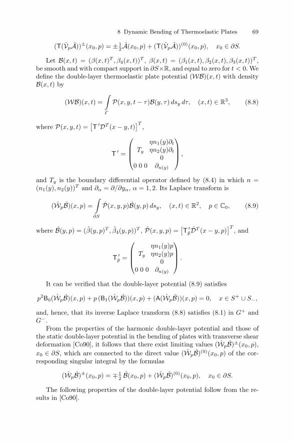
8 Dynamic Bending of Thermoelastic Plates 69
(T(VpA))±(x0, p) = ± 12 A(x0, p) + (T(VpA))(0)(x0, p), x0 ∈ ∂S.
Let B(x, t) = (β(x, t)T , β4(x, t))T , β(x, t) = (β1(x, t), β2(x, t), β3(x, t))
T ,be smooth and with compact support in ∂S×R, and equal to zero for t < 0. Wedefine the double-layer thermoelastic plate potential (WB)(x, t) with densityB(x, t) by
(WB)(x, t) =
∫
Γ
P(x, y, t− τ)B(y, τ) dsy dτ, (x, t) ∈ R3, (8.8)
where P(x, y, t) =[T
′DT (x− y, t)]T
,
T′ =
⎛⎜⎜⎝
Ty
ηn1(y)∂t
ηn2(y)∂t
00 0 0 ∂n(y)
⎞⎟⎟⎠ ,
and Ty is the boundary differential operator defined by (8.4) in which n =(n1(y), n2(y))
T and ∂α = ∂/∂yα, α = 1, 2. Its Laplace transform is
(WpB)(x, p) =
∫
∂S
P(x, y, p)B(y, p) dsy, (x, t) ∈ R2, p ∈ C0, (8.9)
where B(y, p) = (β(y, p)T , β4(y, p))T , P(x, y, p) =
[T
′pDT (x− y, p)
]T, and
T′p =
⎛⎜⎜⎝
Ty
ηn1(y)pηn2(y)p
00 0 0 ∂n(y)
⎞⎟⎟⎠ .
It can be verified that the double-layer potential (8.9) satisfies
p2B0(WpB)(x, p) + p (B1(WpB))(x, p) + (A(WpB))(x, p) = 0, x ∈ S+ ∪ S−,
and, hence, that its inverse Laplace transform (8.8) satisfies (8.1) in G+ andG−.
From the properties of the harmonic double-layer potential and those ofthe static double-layer potential in the bending of plates with transverse sheardeformation [Co90], it follows that there exist limiting values (WpB)±(x0, p),
x0 ∈ ∂S, which are connected to the direct value (WpB)(0)(x0, p) of the cor-responding singular integral by the formulas
(WpB)±(x0, p) = ∓ 12 B(x0, p) + (WpB)(0)(x0, p), x0 ∈ ∂S.
The following properties of the double-layer potential follow from the re-sults in [Co90].

70 I. Chudinovich and C. Constanda
(i) If B ∈ C0,α(∂S), α ∈ (0, 1], then WpB ∈ C∞(S+ ∪ S−).
(ii) In this case, WpB may be extended from S± to S±, respectively, andthe extended vector-valued functions are of class C0,β(S±), with β = α forα ∈ (0, 1) and any β ∈ (0, 1) for α = 1.
We define the operators
W±p : B(x) → (WpB)±(x, p), x ∈ ∂S,
generated by the limiting values (WpB)± of the double-layer potential.
8.5 Solvability of the Time-Dependent BoundaryIntegral Equations
A few more function spaces are necessary. Let κ > 0 and k, l ∈ R.
HL1,k,κ(S±), HL
1,k,κ(S±) HL±1/2,k,κ(∂S), HL
±1/2,k,κ(∂S) : the spaces of all
u(x, p), u4(x, p), x ∈ S±, p ∈ Cκ, e(x, p), e4(x, p), x ∈ ∂S, p ∈ Cκ, which de-fine holomorphic mappings Cκ → H1(S
±), Cκ → H1(S±) Cκ → H±1/2(∂S),
Cκ → H±1/2(∂S), with norms
‖u‖21,k,κ;S± = sup
σ>κ
∞∫
−∞
(1 + |p|2)k‖u(x, p)‖21,p;S± dζ,
‖u4‖21,k,κ;S± = sup
σ>κ
∞∫
−∞
(1 + |p|2)k‖u4(x, p)‖21;S± dζ,
‖e‖2±1/2,k,κ;∂S = sup
σ>κ
∞∫
−∞
(1 + |p|2)k‖e(x, p)‖2±1/2,p;∂S dζ,
‖e4‖2±1/2,k,κ;∂S = sup
σ>κ
∞∫
−∞
(1 + |p|2)k‖e4(x, p)‖2±1/2;∂S dζ.
HL1,k,l,κ(S±) = HL
1,k,κ(S±) × HL1,l,κ(S±), HL
±1/2,k,l,κ(∂S) = HL±1/2,k,κ(∂S) ×
HL±1/2,l,κ(∂S), with norms
‖|U‖|1,k,l,κ;S± = ‖u‖1,k,κ;S± + ‖u4‖1,l,κ;S± ,
‖|E‖|±1/2,k,l,κ;∂S = ‖e‖±1/2,k,κ;∂S + ‖e4‖±1/2,l,κ;∂S .
Let A ∈ HL−1/2,k,l,κ(∂S), F = (ϕT , ϕ4)
T ∈ HL1/2,k,l,κ(∂S), and G =
(gT , g4)T ∈ HL
−1/2,k,l,κ(∂S). We define operators V and V−1 by setting
(VA)(x, p) = (VpA)(x, p), (V−1F )(x, p) = (V−1p F )(x, p), x ∈ ∂S, p ∈ Cκ.

8 Dynamic Bending of Thermoelastic Plates 71
We now define operators K±, W±, and F and their inverses by setting,for x ∈ ∂S,
(K±A)(x, p) = (K±p A)(x, p), ((K±)−1G)(x, p) = ((K±
p )−1G)(x, p),
(W±B)(x, p) = (W±p B)(x, p), ((W±)−1F )(x, p) = ((W±
p )−1F )(x, p),
(FB)(x, p) = (FpB)(x, p), (F−1G)(x, p) = (F−1p G)(x, p).
To derive the fundamental results of this chapter, we need to introduceone last batch of function spaces. Again, let κ > 0 and k, l ∈ R.
HL−1
1,k,κ(G±), HL−1
1,l,κ(G±), HL−1
1,k,l,κ(G±) = HL−1
1,k,κ(G±)×HL−1
1,l,κ(G±) : the spaces
of the inverse Laplace transforms of all the elements of HL1,k,κ(S±), HL
1,l,κ(S±),
HL1,k,l,κ(S±) = HL
1,k,κ(S±) × HL1,l,κ(S±). The norms of u(x, t) = L−1u(x, p),
u4(x, t) = L−1u4(x, p), and U(x, t) = L−1U(x, p) = (u(x, t)T , u4(x, t))T are
‖u‖1,k,κ;G± = ‖u‖1,k,κ;S± , ‖u4‖1,l,κ;G± = ‖u4‖1,l,κ;S± ,
‖|U‖|1,k,l,κ;G± = ‖|U‖|1,k,l,κ;S± .
HL−1
±1/2,k,κ(Γ ), HL−1
±1/2,l,κ(Γ ), HL−1
±1/2,k,l,κ(Γ ) = HL−1
±1/2,k,κ(Γ ) × HL−1
±1/2,l,κ(Γ ) :
the spaces of the inverse transforms of all the elements of HL±1/2,k,κ(∂S),
HL±1/2,l,κ(∂S), HL
±1/2,k,l,κ(∂S) = HL±1/2,k,κ(∂S) × HL
±1/2,l,κ(∂S). The norms
of e(x, t) = L−1e(x, p), e4(x, t) = L−1e4(x, p), E(x, t) = L−1E(x, p) =(e(x, t)T , e4(x, t))
T are
‖e‖±1/2,k,κ;Γ = ‖e‖±1/2,k,κ;∂S , ‖e4‖±1/2,l,κ;Γ = ‖u4‖±1/2,l,κ;∂S ,
‖|E‖|±1/2,k,l,κ;Γ = ‖|E‖|±1/2,k,l,κ;∂S .
In what follows, we extend the use of the symbols γ± to denote also thetrace operators from G± to Γ .
U = U(x, t), U = (uT , u4)T ∈ HL−1
1,0,0,κ(G±), is called a weak solution ofthe corresponding original problem (TD±) if
Υ±(U,W ) = 0, γ±U = F,
where
Υ±(U,W ) =
∞∫
0
a±(u,w) + (∇u4,∇w4)0;S± − (B1/20 ∂tu,B
1/20 ∂tw)0;S±
− χ−1(u4, ∂tw4)0;S± − h2γ(u4,divw)0;S± − η(divu, ∂tw4)0;S± dt,
for all W = W (x, t), W = (wT , w4)T ∈ C∞
0 (G±), that is, for all infinitelysmooth four-component vector-valued functions with compact support in G±
and satisfying γ±W = 0. Also, U ∈ HL−1
1,0,0,κ(G±) is called a weak solution of(TN±) if

72 I. Chudinovich and C. Constanda
Υ±(U,W ) = ±L(W ) ∀W ∈ C∞0 (G±),
where
L(W ) =
∞∫
0
(G,W )0;∂S dt.
The solvability of all these problems was studied in [ChCo05a].The single-layer and double-layer potentials (VA)(x, t) and (WB)(x, t),
(x, t) ∈ R3, with densities vanishing for t < 0, may be defined as the inverse
Laplace transforms of (VA)(x, p) and (WB)(x, p), respectively; that is,
(VA)(x, t) = L−1((VA)(x, p)), (WB)(x, t) = L−1((WB)(x, p)).
These potentials generate boundary operators V,W±,K±, and F defined by
V = L−1VL, W± = L−1W±L, K± = L−1K±L, F = L−1FL.
We seek the solutions of (TD±), in turn, as a single-layer potential and adouble-layer potential; in other words,
U(x, t) = (VA)(x, t), U(x, t) = (WB)(x, t), (x, t) ∈ G±,
with unknown densities A and B. After passing to the limit as (x, t) → Γ ,these representations lead to the systems of boundary integral equations
VA = F, W±B = F, (8.10)
respectively. The same representations for the solutions of (TN±) yield thesystems
K±A = G, FB = G. (8.11)
Theorem 3. For any κ > 0 and k ∈ R, systems (8.10) and (8.11) have uniquesolutions.
Theorem 4. (i) If F ∈ HL−1
1/2,k+1,k+1,κ(Γ ) and A and B are the solutions
of (8.10), then U(x, t) = (VA)(x, t) and U(x, t) = (WB)(x, t) belong to
HL−1
1,k,k,.κ(G±) for any κ > 0, k ∈ R, and
‖|U‖|1,k,k,κ;G± ≤ c‖|F‖|1/2,k+1,k+1,κ;Γ .
(ii) If G ∈ HL−1
−1/2,k+1,k,κ(Γ ) and A and B are the solutions of (8.11), then
U(x, t) = (VA)(x, t) and U(x, t) = (WB)(x, t) belong to HL−1
1,k,k,κ(G±) for anyκ > 0, k ∈ R, and
‖|U‖|1,k,k,κ;G± ≤ c‖|G‖|−1/2,k+1,k,κ;Γ .
(iii) If k ≥ 0, then U(x, t) is the weak solution of (TD±) or (TN±), asappropriate.
These assertions are proved by using the mapping properties of the bound-ary operators and Theorems 1 and 2.

8 Dynamic Bending of Thermoelastic Plates 73
References
[ChCo99] Chudinovich, I., Constanda, C.: Nonstationary integral equations forelastic plates. C.R. Acad. Sci. Paris Ser. I, 329, 1115–1120 (1999).
[ChCo00] Chudinovich, I., Constanda, C.: Variational and Potential Methods inthe Theory of Bending of Plates with Transverse Shear Deformation.Chapman & Hall/CRC, Boca Raton-London-New York-Washington,DC (2000).
[ChCo00a] Chudinovich, I., Constanda, C.: The Cauchy problem in the theory ofplates with transverse shear deformation. Math. Models Methods Appl.Sci., 10, 463–477 (2000).
[ChCo02] Chudinovich, I., Constanda, C.: Boundary integral equations in dynamicproblems for elastic plates. J. Elasticity, 68, 73–94 (2002).
[ChCo03] Chudinovich, I., Constanda, C.: Time-dependent boundary integralequations for multiply connected plates. IMA J. Appl. Math., 68, 507–522 (2003).
[ChCo04] Chudinovich, I., Constanda, C., Colın Venegas, J.: The Cauchy problemin the theory of thermoelastic plates with transverse shear deformation.J. Integral Equations Appl., 16, 321–342 (2004).
[ChCo05] Chudinovich, I., Constanda, C.: Variational and Potential Methods fora Class of Linear Hyperbolic Evolutionary Processes. Springer, London(2005).
[ChCo05a] Chudinovich, I., Constanda, C., Colın Venegas, J.: Solvability of initial-boundary value problems for bending of thermoelasic plates with mixedboundary conditions. J. Math. Anal. Appl., 311, 357–376 (2005).
[ChCo06] Chudinovich, I., Constanda, C., Colın Venegas, J.: On the Cauchy prob-lem for thermoelastic plates. Math. Methods Appl. Sci., 29, 625–636(2006).
[ChDu00] Chudinovich, I., Dumina, O.: Boundary equations in dynamic problemsfor thermoelastic media. Visnyk Kharkiv Nat. Univ. Ser. Math. Appl.Math. Mech., 475, 230–240 (2000).
[Co90] Constanda, C.: A Mathematical Analysis of Bending of Plates withTransverse Shear Deformation. Longman/Wiley, Harlow-New York(1990).
[KGBB78] Kupradze, V.D., Gegelia, T.G., Basheleishvili, M.O., Burchuladze, T.V.:Three-dimensional Problems of the Mathematical Theory of Elasticityand Thermoelasticity. P. Noordhoff, Amsterdam (1978).
[ScTa93] Schiavone, P., Tait, R.J.: Thermal effects in Mindlin-type plates. Quart.J. Mech. Appl. Math., 46, 27–39 (1993).
[ScTa95] Schiavone, P., Tait, R.J.: Steady time-harmonic oscillations in a linearthermoelastic plate model. Quart. Appl. Math., 53, 215–233 (1995).


9
Direct Methods in the Theory ofThermoelastic Plates
I. Chudinovich and C. Constanda
University of Tulsa, OK, USA; [email protected],[email protected]
9.1 The Mathematical Model
Consider a plate occupying a region S × [−h0/2, h0/2] in R3, where S is a
domain in R2 with a simple, closed C2-boundary ∂S and h0 = const > 0 is
the thickness.We write G = S × (0,∞), Γ = ∂S × (0,∞), and x = (x1, x2), and assume
that the material is homogeneous and isotropic with Lame constants λ andµ, density ρ, and heat-related (positive) constants γ, η, and χ.
The displacements and thermal “moment” in the plate are denoted by
u(x, t) =(x3u1(x, t), x3u2(x, t), u3(x, t)
)T,
u4(x, t) =1
h2h0
h0/2∫
−h0/2
x3θ(x, x3, t) dx3, h2 =h2
0
12,
where U = (u1, u2, u3, u4)T = (uT , u4)
T and θ(x, x3, t) is the temperature.Applying the procedure of averaging over the thickness, we arrive at the
system of governing equations
B0∂2tU(x, t) + B1∂tU(x, t) + AU(x, t) = 0, (x, t) ∈ G, (9.1)
where B0 = diag ρh2, ρh2, ρ, 0,
B1 =
⎛⎜⎜⎝
0 0 0 00 0 0 00 0 0 0η∂1 η∂2 0 χ−1
⎞⎟⎟⎠ , A =
⎛⎜⎜⎝
Ah2γ∂1
h2γ∂2
00 0 0 −∆
⎞⎟⎟⎠ ,
A =
⎛⎝
−h2µ∆− h2(λ+ µ)∂21 + µ −h2(λ+ µ)∂1∂2 µ∂1
−h2(λ+ µ)∂1∂2 −h2µ∆− h2(λ+ µ)∂22 + µ µ∂2
−µ∂1 −µ∂2 −µ∆
⎞⎠ ,

76 I. Chudinovich and C. Constanda
∂t = ∂/∂t, and ∂α = ∂/∂xα, α = 1, 2.Along with these equations we consider the boundary moment-stress op-
erator
T =
⎛⎝h2[(λ+ 2µ)n1∂1 + µn2∂2] h2(λn1∂2 + µn2∂1) 0
h2(µn1∂2 + λn2∂1) h2[(λ+ 2µ)n2∂2 + µn1∂1] 0µn1 µn2 µ∂n
⎞⎠ ,
where n = (n1, n2)T is the outward unit normal to ∂S and ∂n = ∂/∂n.
To the governing equations, we adjoin either Dirichlet boundary conditions
U = F = (fT , f4)T on Γ (9.2)
or Neumann boundary conditions
T U =
(Tu− h2γnu4
∂nu4
)= G = (gT , g4)
T on Γ , (9.3)
and (without loss of generality) homogeneous initial conditions
U(x, 0) = 0, (∂tu)(x, 0) = 0, x ∈ S. (9.4)
For the purpose of this discussion, we distinguish between the interior andexterior domains with respect to the boundary ∂S, denoting the former byS+ and the latter by S−. Obviously, we also write G± = S± × (0,∞).
Two classical initial-boundary value problems are considered here, as fol-lows:
(TD±): find U ∈ C2(G±)∩C1(G±) satisfying (9.1) in G±, (9.2) on Γ , and(9.3) in S±.
(TN±): find U ∈ C2(G±)∩C1(G±) satisfying (9.1) in G±, (9.3) on Γ , and(9.4) in S±.
9.2 The Laplace-Transformed Problems
With the notation LU(x, t) = U(x, p), we apply the Laplace transformationL to our initial-value problems and reduce them to corresponding boundaryvalue problems:
(TD±p ): Find U ∈ C2(S±) ∩ C1(S±) such that
p2B0U + p (B1U) + (AU) = 0 in S±,
U = F on ∂S.
(TN±p ): Find U ∈ C2(S±) ∩ C1(S±) such that
p2B0U + p (B1U) + (AU) = 0 in S±,
T ±U = G on ∂S.

9 Direct Methods in the Theory of Thermoelastic Plates 77
To study these problems, we adopt all definitions of functions spaces,norms, inner products, and trace operators given in [ChCo1]. We also recallthe sesquilinear form for U = (uT , u4)
T , W = (wT , w4)T ∈ H1,p(S
±) definedby
Υ±,p(U , W ) = a±(u, w) + (∇u4,∇w4)0;∂S± + p2(B1/20 u, B
1/20 w)0;S±
+ χ−1p (u4, w4)0;S± − h2γ(u4,div w)0;S± + ηp (div u, w4)0,S± ,
where B0 = diag ρh2, ρh2, ρ, a±(u, w) = 2∫
S±
E(u, w) dx, and E is the
quadratic form of the internal static energy density.For G ∈ H−1/2,p(∂S) and W ∈ H1/2,p(∂S), we define
L(W ) = (G, W )0;∂S = (g, w)0;∂S + (g4, w4)0;∂S .
We can now formulate the variational Laplace-transformed problems.
(TD±p ): Find U ∈ H1,p(S
±) such that
Υ±,p(U , W ) = 0 ∀W ∈[H1(S
±)]4,
γ±U = F .
(TN±p ): Find U ∈ H1,p(S
±) such that
Υ±,p(U , W ) = ±L(W ) ∀W ∈[H1(S
±)]4.
Let Cκ = p = σ + iζ ∈ C : σ > κ.
Theorem 1. (i) If F (x, p) ∈ H1/2,p(∂S), p ∈ Cκ, κ > 0, then (TD±p ) have
unique solutions U(x, p) ∈ H1,p(S±), and if F : Cκ → H1/2(∂S) is holomor-
phic, then so are U : Cκ → H1(S±).
(ii) If G(x, p) ∈ H−1/2,p(∂S), p ∈ Cκ, κ > 0, then (TN±p ) have unique
solutions U(x, p) ∈ H1,p(S±), and if G : Cκ → H−1/2(∂S) is holomorphic,
then so are U : Cκ → H1(S±).
9.3 The Analogs of Green’s Formulas in the TransformDomain
Let
p ∈ Cκ, κ > 0,
Lp = p2B0 + pB1 + A,
U ∈ C2(S±) ∩ C1(S±), W ∈ C1(S±) ∩ C(S±), Φ = γ±W .
In S−, suppose, for example, that

78 I. Chudinovich and C. Constanda
|U(x, p)| +
4∑
i=1
|∇ui(x, p)| ≤ c
(1 + |x|)1+ε,
|W (x, p)| +
4∑
i=1
|∇wi(x, p)| ≤ c
(1 + |x|)1+ε,
where c = c(p) > 0 and ε > 0. Then the analog of Green’s first formula (Bettiformula) for Lp is written as
(LpU , W )0;S± = ∓(T ±p U , Φ)0;∂S + Υ±,p(U , W ).
The formal adjoint to Lp is
L′p = p2
B0 + pB′1 + A
′,
where
B′1 =
⎛⎜⎜⎝
0 0 0 −η∂1
0 0 0 −η∂2
0 0 0 00 0 0 χ−1
⎞⎟⎟⎠ , A
′ =
⎛⎜⎜⎝
A000
0 0 0 −∆
⎞⎟⎟⎠ .
Then the analog of Green’s second formula (reciprocity relation) takes theform
(LpU , W )0;S± − (U , L′pW )0;S± = ∓
[(T ±
p U , Φ)0;∂S − (F , (T ′p )±W )0;∂S
],
where
T ′p =
⎛⎜⎜⎝
Ty
ηn1(y)pηn2(y)p
00 0 0 ∂n(y)
⎞⎟⎟⎠
and F = γ±U .Finally, the analog of Green’s third formula (Somigliana formula) is
U(x) = ±∫
∂S
D(x− y, p)(T ±p U)(y) dsy −
∫
∂S
P(x, y, p)U(y) dsy
+
∫
S±
D(x− y, p)(LpU)(y) dy,
where P(x, y, p) =[T ′
p DT (x− y, p)]T
and D(x, p) is the Laplace transform ofa matrix D(x, t) of fundamental solutions for (9.1).
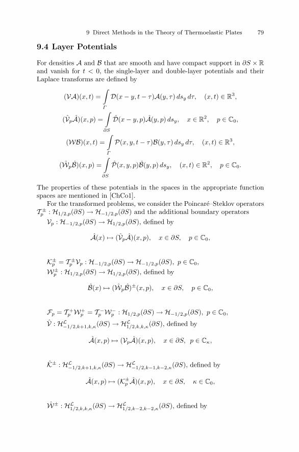
9 Direct Methods in the Theory of Thermoelastic Plates 79
9.4 Layer Potentials
For densities A and B that are smooth and have compact support in ∂S × R
and vanish for t < 0, the single-layer and double-layer potentials and theirLaplace transforms are defined by
(VA)(x, t) =
∫
Γ
D(x− y, t− τ)A(y, τ) dsy dτ, (x, t) ∈ R3,
(VpA)(x, p) =
∫
∂S
D(x− y, p)A(y, p) dsy, x ∈ R2, p ∈ C0,
(WB)(x, t) =
∫
Γ
P(x, y, t− τ)B(y, τ) dsy dτ, (x, t) ∈ R3,
(WpB)(x, p) =
∫
∂S
P(x, y, p)B(y, p) dsy, (x, t) ∈ R2, p ∈ C0.
The properties of these potentials in the spaces in the appropriate functionspaces are mentioned in [ChCo1].
For the transformed problems, we consider the Poincare–Steklov operatorsT ±
p : H1/2,p(∂S) → H−1/2,p(∂S) and the additional boundary operators
Vp : H−1/2,p(∂S) → H1/2,p(∂S), defined by
A(x) → (VpA)(x, p), x ∈ ∂S, p ∈ C0,
K±p = T ±
p Vp : H−1/2,p(∂S) → H−1/2,p(∂S), p ∈ C0,
W±p : H1/2,p(∂S) → H1/2,p(∂S), defined by
B(x) → (WpB)±(x, p), x ∈ ∂S, p ∈ C0,
Fp = T +p W+
p = T −p W−
p : H1/2,p(∂S) → H−1/2,p(∂S), p ∈ C0,
V : HL−1/2,k+1,k,κ(∂S) → HL
1/2,k,k,κ(∂S), defined by
A(x, p) → (VpA)(x, p), x ∈ ∂S, p ∈ Cκ,
K± : HL−1/2,k+1,k,κ(∂S) → HL
−1/2,k−1,k−2,κ(∂S), defined by
A(x, p) → (K±p A)(x, p), x ∈ ∂S, κ ∈ C0,
W± : HL1/2,k,k,κ(∂S) → HL
1/2,k−2,k−2,κ(∂S), defined by
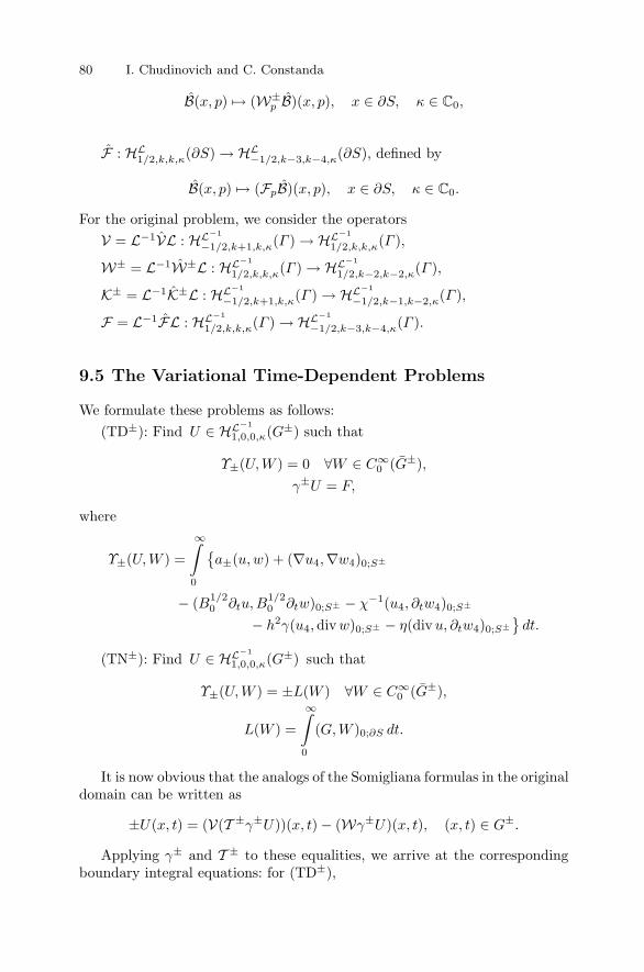
80 I. Chudinovich and C. Constanda
B(x, p) → (W±p B)(x, p), x ∈ ∂S, κ ∈ C0,
F : HL1/2,k,k,κ(∂S) → HL
−1/2,k−3,k−4,κ(∂S), defined by
B(x, p) → (FpB)(x, p), x ∈ ∂S, κ ∈ C0.
For the original problem, we consider the operators
V = L−1VL : HL−1
−1/2,k+1,k,κ(Γ ) → HL−1
1/2,k,k,κ(Γ ),
W± = L−1W±L : HL−1
1/2,k,k,κ(Γ ) → HL−1
1/2,k−2,k−2,κ(Γ ),
K± = L−1K±L : HL−1
−1/2,k+1,k,κ(Γ ) → HL−1
−1/2,k−1,k−2,κ(Γ ),
F = L−1FL : HL−1
1/2,k,k,κ(Γ ) → HL−1
−1/2,k−3,k−4,κ(Γ ).
9.5 The Variational Time-Dependent Problems
We formulate these problems as follows:
(TD±): Find U ∈ HL−1
1,0,0,κ(G±) such that
Υ±(U,W ) = 0 ∀W ∈ C∞0 (G±),
γ±U = F,
where
Υ±(U,W ) =
∞∫
0
a±(u,w) + (∇u4,∇w4)0;S±
− (B1/20 ∂tu,B
1/20 ∂tw)0;S± − χ−1(u4, ∂tw4)0;S±
− h2γ(u4,divw)0;S± − η(divu, ∂tw4)0;S±
dt.
(TN±): Find U ∈ HL−1
1,0,0,κ(G±) such that
Υ±(U,W ) = ±L(W ) ∀W ∈ C∞0 (G±),
L(W ) =
∞∫
0
(G,W )0;∂S dt.
It is now obvious that the analogs of the Somigliana formulas in the originaldomain can be written as
±U(x, t) = (V(T ±γ±U))(x, t) − (Wγ±U)(x, t), (x, t) ∈ G±.
Applying γ± and T ± to these equalities, we arrive at the correspondingboundary integral equations: for (TD±),

9 Direct Methods in the Theory of Thermoelastic Plates 81
VA = W∓F, A = T ±F, (9.5)
and for (TN±),FB = K∓G, B = (T ±)−1G. (9.6)
The main result, obtained by combining the mapping properties of theboundary operators introduced above and Theorem 1, is contained in thenext assertion.
Theorem 2. Systems (9.5) and (9.6) have unique solutions for any κ > 0,k ∈ R.
(i) If F ∈ HL−1
1/2,k+1,k+1,κ(Γ ), then
±U = VA − WF ∈ HL−1
1,k,k,κ(G±), κ > 0, k ∈ R,
‖|U‖|1,k,k,κ;G± ≤ c‖|F‖|1/2,k+1,k+1,κ;Γ .
(ii) If G ∈ HL−1
−1/2,k+1,k,κ(Γ ), then
±U = VG− WB ∈ HL−1
1,k,k,κ(G±), k > 0, k ∈ R,
‖|U‖|1,k,k,κ;G± ≤ c‖|G‖|−1/2,k+1,k,κ;Γ .
(iii) If k ≥ 0, then U is the (unique) weak solution of (TD±) or (TN±),as appropriate.
References
[ChCo1] Chudinovich, I., Constanda, C.: Layer potentials in dynamic bending ofthermoelastic plates. In: Constanda, C., Potapenko, S. (eds.), IntegralMethods in Science and Engineering: Techniques and Applications (thisvolume). Birkhauser, Boston, MA (2007), pp. 67–77.


10
The Dirichlet Problem for the PlaneDeformation of a Thin Plate on an ElasticFoundation
I. Chudinovich, C. Constanda, D. Doty, W. Hamill, and S. Pomeranz
University of Tulsa, OK, USA; [email protected],[email protected], [email protected],[email protected], [email protected]
10.1 Prerequisites
We consider an elastic plate that occupies a region S ⊂ R2 bounded by a
simple, closed, C2-contour ∂S. The extensional motion of the plate is charac-terized by a displacement field of the form
u(x) =(u1(x), u2(x)
)T,
where x = (x1, x2) and the superscript T denotes matrix transposition. Whenthe plate lies on an elastic foundation, the response of the latter is modeled bythe matrix K = diagk, k, where k > 0 is the foundation’s elastic coefficient.
The boundary value problem for prescribed displacements on ∂S in thecase of equilibrium under in-plane external forces
q(x) =(q1(x), q2(x)
)T
consists of the governing equations and Dirichlet boundary conditions:
Zu = Au−Ku = q in S,u = f on ∂S,
(10.1)
where
A =
(µ∆+ (λ+ µ)∂2
1 (λ+ µ)∂1∂2
(λ+ µ)∂1∂2 µ∆+ (λ+ µ)∂22
)
and ∂α = ∂/∂xα, α = 1, 2.We introduce the Sobolev spaces Hm(S), H(S), and Hm(∂S), m ∈ R
[DuLi76]. For q ∈ H−1(S) and f ∈ H1/2(∂S), we can use standard functionalanalysis methods [DuLi76] to prove that problem (10.1) has a unique weaksolution in H1(S). Without loss of generality, we focus on the case q = 0, since
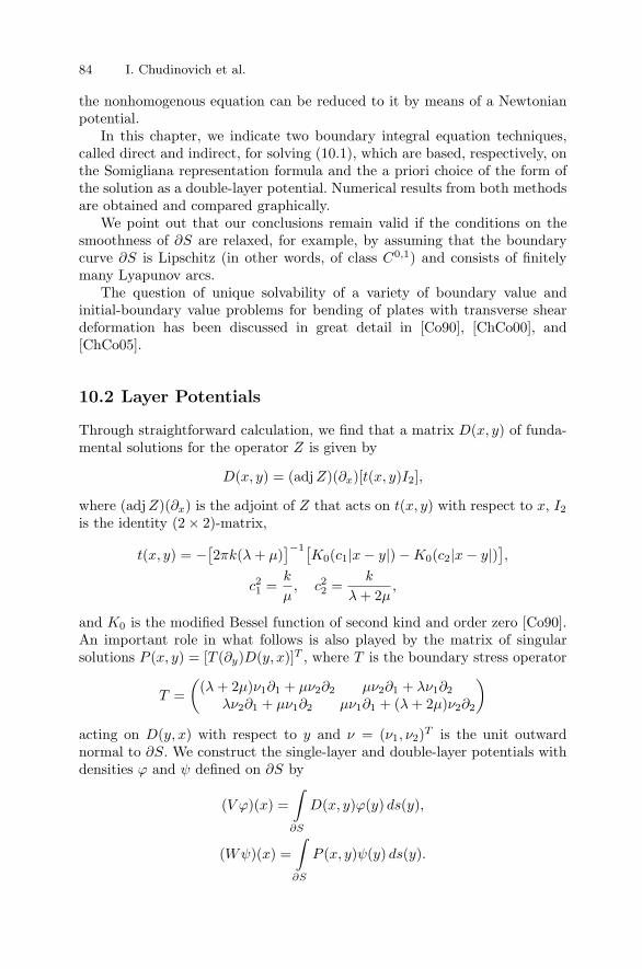
84 I. Chudinovich et al.
the nonhomogenous equation can be reduced to it by means of a Newtonianpotential.
In this chapter, we indicate two boundary integral equation techniques,called direct and indirect, for solving (10.1), which are based, respectively, onthe Somigliana representation formula and the a priori choice of the form ofthe solution as a double-layer potential. Numerical results from both methodsare obtained and compared graphically.
We point out that our conclusions remain valid if the conditions on thesmoothness of ∂S are relaxed, for example, by assuming that the boundarycurve ∂S is Lipschitz (in other words, of class C0,1) and consists of finitelymany Lyapunov arcs.
The question of unique solvability of a variety of boundary value andinitial-boundary value problems for bending of plates with transverse sheardeformation has been discussed in great detail in [Co90], [ChCo00], and[ChCo05].
10.2 Layer Potentials
Through straightforward calculation, we find that a matrix D(x, y) of funda-mental solutions for the operator Z is given by
D(x, y) = (adjZ)(∂x)[t(x, y)I2],
where (adjZ)(∂x) is the adjoint of Z that acts on t(x, y) with respect to x, I2is the identity (2 × 2)-matrix,
t(x, y) = −[2πk(λ+ µ)
]−1[K0(c1|x− y|) −K0(c2|x− y|)
],
c21 =k
µ, c22 =
k
λ+ 2µ,
and K0 is the modified Bessel function of second kind and order zero [Co90].An important role in what follows is also played by the matrix of singularsolutions P (x, y) = [T (∂y)D(y, x)]T , where T is the boundary stress operator
T =
((λ+ 2µ)ν1∂1 + µν2∂2 µν2∂1 + λν1∂2
λν2∂1 + µν1∂2 µν1∂1 + (λ+ 2µ)ν2∂2
)
acting on D(y, x) with respect to y and ν = (ν1, ν2)T is the unit outward
normal to ∂S. We construct the single-layer and double-layer potentials withdensities ϕ and ψ defined on ∂S by
(V ϕ)(x) =
∫
∂S
D(x, y)ϕ(y) ds(y),
(Wψ)(x) =
∫
∂S
P (x, y)ψ(y) ds(y).

10 Thin Plate on an Elastic Foundation 85
If ϕ ∈ H−1/2(∂S) and ψ ∈ H1/2(∂S), then V ϕ, Wψ ∈ H1(S). Let γ be thetrace operator that maps H1(S) continuously onto H1/2(∂S). We can nowdefine boundary operators V + and W+ by
V +ϕ = γ(V ϕ),
W+ψ = γ(Wψ).
It is easily seen that V + is an integral operator with a weakly singular kernel,and that
W+ = −12 I +W0,
where I is the identity operator and W0 is an integral operator with a sin-gular kernel, which means that the integral in its definition is understood asprincipal value.
Theorem 1. The operators
V + : H−1/2(∂S) → H1/2(∂S),
W+ : H1/2(∂S) → H1/2(∂S)
are bijective.
10.3 Boundary Integral Equations
10.3.1 The Indirect Method
We seek the solution of (10.1) in the form
u(x) = (Wψ)(x), x ∈ S,
with an unknown density ψ. As x tends to ∂S, we obtain the system of singularintegral equations
W+ψ = f (10.2)
or−1
2 ψ +W0ψ = f.
Theorem 2. If f ∈ H1/2(∂S), then (10.2) has a unique solution ψ ∈H1/2(∂S). In this case, u = Wψ ∈ H1(S) is the weak (variational) solutionof (10.1).

86 I. Chudinovich et al.
10.3.2 The Direct Method
Adapting the procedure for deriving Green’s third formula for the Laplaceequation to our case, we obtain the so-called Somigliana formula. If u ∈C2(S) ∩ C1(S) satisfies Zu = 0 in S, then
∫
∂S
[D(x, y)(Tu)(y) − P (x, y)u(y)
]ds(y) =
u(x), x ∈ S,12 u(x), x ∈ ∂S.
(10.3)
According to the second equation in (10.1), γu = f , so representation(10.3) implies that
V +ϕ−W+f = f
orV +ϕ =
(12 I +W0
)f, (10.4)
where ϕ = Tu.We remark that, in contrast to the indirect method, where the density ψ
has no physical significance, here ϕ is the boundary stress vector computedfrom the solution of the Dirichlet problem. According to Theorem 1, we canextend the operators in (10.4) by continuity to the corresponding Sobolevspaces.
Theorem 3. If f ∈ H1/2(∂S), then system (10.4) has a unique solution ϕ ∈H−1/2(∂S). In this case, u = V ϕ ∈ H1(S) is the weak (variational) solutionof (10.1).
10.4 Illustrative Example
We considered a square steel floor that occupies the region S = [0, 1] × [0, 1],for which
λ = 1.141 × 10⁸, µ = 8.262 × 10⁷,
with all units given in SI (kg, m, s). We assumed that this floor lies on top ofa flat foundation with elastic coefficient
k = 4 × 10⁷.
We chose the boundary condition f = γu to be
u(x1, 0) =(0, 0.01 sin(πx1)
)T,
u(x1, 1) =(0, −0.01 sin(πx1)
)T,
u(0, x2) =(
− 0.01 sin(πx2), 0)T,
u(1, x2) =(0.01 sin(πx2), 0
)T.

10 Thin Plate on an Elastic Foundation 87
Fig. 10.1. Component u1 by the indirect method.
Fig. 10.2. Component u2 by the indirect method.
Fig. 10.3. Component u1 by the direct method.

88 I. Chudinovich et al.
Fig. 10.4. Component u2 by the direct method.
Using MATEMATICA, we computed D(x, y) and P (x, y) symbolically andemployed Gaussian quadrature to calculate the Cauchy principal values, andcubic splines to approximate the solutions of the boundary integral equations.
As Figures 10.1–10.4 show, the results yielded by both the direct and theindirect methods are very good approximations, which means that from acomputational viewpoint, the choice of one over the other is not significant.However, the practitioner might prefer the direct method because it is linkedto the physics of the model in that the unknown potential density representsthe stress vector on the boundary contour.
References
[ChCo00] Chudinovich, I., Constanda, C.: Variational and Potential Methods inthe Theory of Bending of Plates with Transverse Shear Deformation.Chapman & Hall/CRC, Boca Raton-London-New York-Washington, DC(2000).
[ChCo05] Chudinovich, I., Constanda, C.: Variational and Potential Methods fora Class of Linear Hyperbolic Evolutionary Processes. Springer, London(2005).
[Co90] Constanda, C.: A Mathematical Analysis of Bending of Plates with Trans-verse Shear Deformation. Longman/Wiley, Harlow-New York (1990).
[DuLi76] Duvaut, G., Lions, J.-L.: Inequalities in Mechanics and Physics. Springer,Berlin (1976).
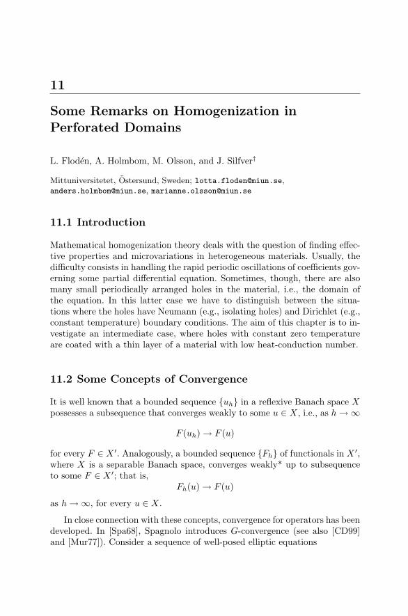
11
Some Remarks on Homogenization inPerforated Domains
L. Floden, A. Holmbom, M. Olsson, and J. Silfver†
Mittuniversitetet, Ostersund, Sweden; [email protected],[email protected], [email protected]
11.1 Introduction
Mathematical homogenization theory deals with the question of finding effec-tive properties and microvariations in heterogeneous materials. Usually, thedifficulty consists in handling the rapid periodic oscillations of coefficients gov-erning some partial differential equation. Sometimes, though, there are alsomany small periodically arranged holes in the material, i.e., the domain ofthe equation. In this latter case we have to distinguish between the situa-tions where the holes have Neumann (e.g., isolating holes) and Dirichlet (e.g.,constant temperature) boundary conditions. The aim of this chapter is to in-vestigate an intermediate case, where holes with constant zero temperatureare coated with a thin layer of a material with low heat-conduction number.
11.2 Some Concepts of Convergence
It is well known that a bounded sequence uh in a reflexive Banach space Xpossesses a subsequence that converges weakly to some u ∈ X, i.e., as h → ∞
F (uh) → F (u)
for every F ∈ X ′. Analogously, a bounded sequence Fh of functionals in X ′,where X is a separable Banach space, converges weakly* up to subsequenceto some F ∈ X ′; that is,
Fh(u) → F (u)
as h → ∞, for every u ∈ X.
In close connection with these concepts, convergence for operators has beendeveloped. In [Spa68], Spagnolo introduces G-convergence (see also [CD99]and [Mur77]). Consider a sequence of well-posed elliptic equations

90 L. Floden, A. Holmbom, M. Olsson, and J. Silfver
−∇ · (Ah(x)∇uh(x)) = f(x) in Ω, (11.1)
uh(x) = 0 on ∂Ω.
G-convergence of Ah to B means that
uh u in W 1,20 (Ω)
andAh∇uh B∇u in L2(Ω)N ,
where u solves
−∇ · (B(x)∇u(x)) = f(x) in Ω,
u(x) = 0 on ∂Ω.
For the special case of periodic homogenization we have
Ah(x) = A(xε
),
where A is a positive definite matrix that is periodic with respect to the unitcube Y and ε = ε(h) → 0 for h → ∞. In this case, the limit operator Bis a constant matrix that can be computed by solving a partial differentialequation defined on a representative unit Y ; see [CD99].
All modes of convergence discussed above have the common feature thatthe limit, whether a function or an operator, is of the same character asthe elements in the sequence converging to this limit. In 1986, an importantcompactness result of a completely different kind was discovered by Nguetseng;see [Ngu89]. He proved that a bounded sequence uε in L2(Ω) possesses alimit in L2(Ω × Y ) in a certain weak sense. More precisely, for admissiblev : Ω×Y → R, that is, sufficiently smooth and periodic in the second variable,and ε passing to zero, it holds, up to a subsequence, that
∫
Ω
uε(x)v(x,x
ε
)dx →
∫
Ω
∫
Y
u0(x, y)v(x, y) dydx. (11.2)
The most frequently used space of admissible test functions is L2(Ω;C♯(Y )).This compactness result simplifies many homogenization procedures since itenables us to characterize two-scale limits for gradients of bounded sequencesin W 1,2(Ω). This means that it is made precise how such two-scale limitsdepend on the microscale variable y. For uε a bounded sequence in W 1,2(Ω)and v admissible we get, still up to a subsequence, that, as ε → 0,
∫
Ω
∇uε(x)v(x,x
ε
)dx →
∫
Ω
∫
Y
(∇u(x) + ∇yu1(x, y))v(x, y) dydx, (11.3)
where u is the weak W 1,2(Ω)-limit to uε and u1 ∈ L2(Ω;W 1,2♯ (Y )/R).

11 Some Remarks on Homogenization in Perforated Domains 91
In [Ngu89], this result is used to develop a very straightforward homog-enization procedure for elliptic equations. The approach is simply to maketwo suitable choices of test functions in the weak formulation of (11.1) andto apply (11.3). One of the classes of test functions gives us the appropriatehomogenized problem and the other the corresponding local problem definedon Y , the solution of which contains the necessary information to computethe homogenized coefficient B.
11.3 Two-Scale Convergence for Perforated Domains
We have already given an example of one of the main difficulties in homog-enization theory that consists in the analysis of partial differential equationswith rapidly oscillating coefficients. The second most common complicationencountered in the study of periodic structures is that of a domain perforatedby many small periodically arranged holes. This difficulty is usually overcomeby extending functions from the perforated domains, where they are originallydefined, to a somewhat larger domain, where the holes have been filled in. Toget rid of the irrelevant information provided by the functions’ extensions tothe holes, we need cutoff functions.
We introduce a class of smooth functions that approaches cutoff functionsin the limit. Let Y H be an open set in Y ⊂ R
2,
Y δ =y ∈ Y − Y H
∣∣d(y, Y H) < δ
for fixed δ > 0, andY ∗ = Y − Y H − Y δ;
see Figure 11.1.
Fig. 11.1. The unit cube Y .
We define a sequence of functions kh ∈ C♯(Y ) such that
⎧⎨⎩kh(y) = qh > 0 in Y H ,qh < kh(y) < 1 in Y δ,kh(y) = 1 in Y ∗.
Furthermore, kh is strictly increasing with d(y, Y H); e.g.,

92 L. Floden, A. Holmbom, M. Olsson, and J. Silfver
kh(y) = δ−h(1 − qh)d(y, Y H)h + qh,
within Y δ, andkh → χY ∗ in Lp
♯ (Y )
for any p > 0 when h → ∞. Finally, we introduce the sets
Ωε = Ω ∩
x ∈ RN
∣∣∣χY ∗
(x
ε
)= 1
∪ Pε, (11.4)
Ω′ε = Ω ∩
x ∈ R
N∣∣∣χY ∗∪Y δ
(x
ε
)= 1
∪ Pε,
Ωε,δ = Ω′ε − Ωε,
where Pε simply means the part of the perforationsx ∈ R
N∣∣χY ∗
(xε
)= 0
that cuts ∂Ω and lies within Ω. This is illustrated in Figure 11.2, where Ωε
is the white area, Ω′ε is the white area together with the gray area, and Ωε,δ
is the grey area.
Fig. 11.2. The domain Ω.
Proposition 1. Let uε be a sequence in L2 (Ω) such that √
kh(xε )uε(x)
and uε are bounded in L2 (Ω′ε) and L2 (Ω − Ω′
ε), respectively. Then, up to
a subsequence,
∫
Ω′ε
uε(x)kh
(x
ε
)v
(x,
x
ε
)dx →
∫
Ω
∫
Y ∗
u0(x, y)v(x, y) dydx,
as h → ∞, for any admissible test function v, where u0 ∈ L2(Ω × Y ) is the
two-scale limit for a sequence of extensions of uε|Ωεto Ω.
Proof. Obviously, uε|Ωεis bounded in L2(Ωε), and thus, we can choose a
sequence uε of extensions that is bounded in L2(Ω). Hence, for a suitablesubsequence,
∫
Ω
uε(x)χY ∗
(x
ε
)v
(x,
x
ε
)dx →
∫
Ω
∫
Y
u0(x, y)χY ∗(y)v(x, y) dydx,
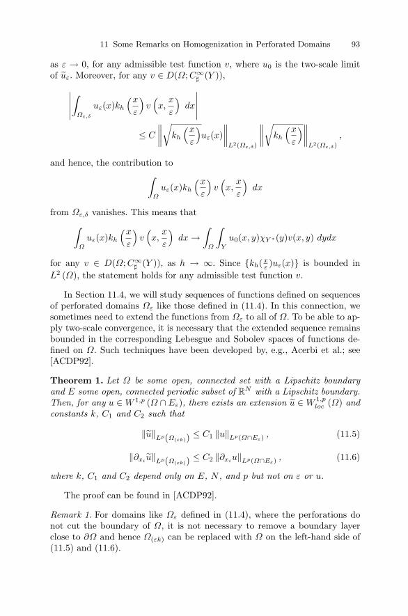
11 Some Remarks on Homogenization in Perforated Domains 93
as ε → 0, for any admissible test function v, where u0 is the two-scale limitof uε. Moreover, for any v ∈ D(Ω;C∞
♯ (Y )),
∣∣∣∣∣
∫
Ωε,δ
uε(x)kh
(x
ε
)v(x,
x
ε
)dx
∣∣∣∣∣
≤ C
∥∥∥∥√
kh
(x
ε
)uε(x)
∥∥∥∥L2(Ωε,δ)
∥∥∥∥√
kh
(x
ε
)∥∥∥∥L2(Ωε,δ)
,
and hence, the contribution to
∫
Ω
uε(x)kh
(x
ε
)v(x,
x
ε
)dx
from Ωε,δ vanishes. This means that
∫
Ω
uε(x)kh
(x
ε
)v(x,
x
ε
)dx →
∫
Ω
∫
Y
u0(x, y)χY ∗(y)v(x, y) dydx
for any v ∈ D(Ω;C∞♯ (Y )), as h → ∞. Since kh(x
ε )uε(x) is bounded in
L2 (Ω), the statement holds for any admissible test function v.
In Section 11.4, we will study sequences of functions defined on sequencesof perforated domains Ωε like those defined in (11.4). In this connection, wesometimes need to extend the functions from Ωε to all of Ω. To be able to ap-ply two-scale convergence, it is necessary that the extended sequence remainsbounded in the corresponding Lebesgue and Sobolev spaces of functions de-fined on Ω. Such techniques have been developed by, e.g., Acerbi et al.; see[ACDP92].
Theorem 1. Let Ω be some open, connected set with a Lipschitz boundaryand E some open, connected periodic subset of R
N with a Lipschitz boundary.Then, for any u ∈ W 1,p (Ω ∩ Eε), there exists an extension u ∈ W 1,p
loc (Ω) andconstants k, C1 and C2 such that
‖u‖Lp(Ω(εk)) ≤ C1 ‖u‖Lp(Ω∩Eε) , (11.5)
‖∂xiu‖Lp(Ω(εk)) ≤ C2 ‖∂xi
u‖Lp(Ω∩Eε) , (11.6)
where k, C1 and C2 depend only on E, N , and p but not on ε or u.
The proof can be found in [ACDP92].
Remark 1. For domains like Ωε defined in (11.4), where the perforations donot cut the boundary of Ω, it is not necessary to remove a boundary layerclose to ∂Ω and hence Ω(εk) can be replaced with Ω on the left-hand side of(11.5) and (11.6).

94 L. Floden, A. Holmbom, M. Olsson, and J. Silfver
Applying these extension techniques to a sequence of functions boundedin W 1,2 (Ωε), we obtain the next assertion.
Proposition 2. Let uε be a sequence of functions in W 1,20 (Ω′
ε) such that
√
kh(xε )∇uε(x) is bounded in L2 (Ω′
ε)N
. Then there exists a sequence offunctions uε in W 1,2 (Ω) such that uε = uε in Ωε and, up to a subsequence,∫
Ω
uε(x)kh
(x
ε
)v(x,
x
ε
)dx →
∫
Ω
∫
Y
u(x)χY ∗(y)v(x, y) dy dx (11.7)
and ∫
Ω
∇uε(x)kh
(x
ε
)v(x,
x
ε
)dx → (11.8)
∫
Ω
∫
Y
(∇u(x) + ∇yu1(x, y))χY ∗(y)v(x, y) dy dx,
as h → ∞, for any admissible test function v, where u is the weak W 1,2(Ω)-limit to uε and u1 ∈ L2(Ω;W 1,2
♯ (Y )/R).
Proof. Let
wh(x) =
√kh
(x
ε
)∇uε(x).
Then, up to a subsequence,∫
Ω
wh(x)kh
(x
ε
)v(x,
x
ε
)dx →
∫
Ω
∫
Y
w0(x, y)χY ∗(y)v(x, y) dy dx,
as h → ∞, for any admissible v and some w0 ∈ L2(Ω×Y )N . It is obvious that
the restriction of wh to Ωε is equal to ∇uε and is bounded in L2 (Ωε)N
. Bythe assumptions on kh and the Poincare inequality for periodically perforateddomains with homogeneous Dirichlet boundary conditions on the holes, weobtain
‖uε‖L2(Ω) ≤ Cε ‖∇uε‖L2(Ω)N ≤ Cε√qh
∥∥∥∥√
kh
(x
ε
)∇uε(x)
∥∥∥∥L2(Ω)N
≤ C
for ε = qh, and thus, uε|Ωε is bounded in W 1,2 (Ωε). Hence, Proposition 1
and Theorem 1 are applicable and (11.7) and (11.8) follow. The loss of thesecond scale in the two-scale limit in (11.7) is due to the strong convergenceof uε in L2 (Ω).
11.4 Homogenization in Perforated Domains
Our aim in this section is to discuss the connection between homogenizationof mixed problems and pure Dirichlet problems in periodically perforated do-mains. Let us first consider the homogenization of a mixed linear elliptic prob-lem with homogeneous boundary data. This may be considered as a model for
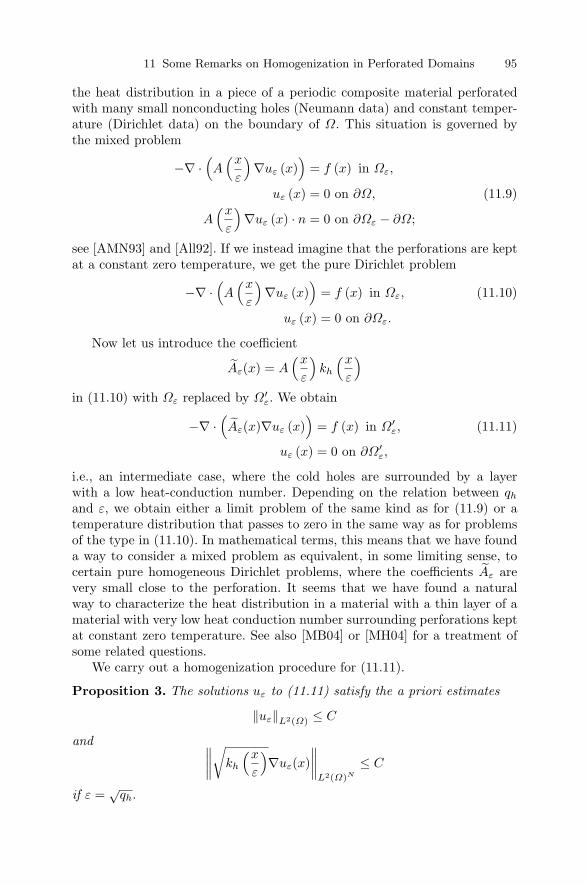
11 Some Remarks on Homogenization in Perforated Domains 95
the heat distribution in a piece of a periodic composite material perforatedwith many small nonconducting holes (Neumann data) and constant temper-ature (Dirichlet data) on the boundary of Ω. This situation is governed bythe mixed problem
−∇ ·(A
(x
ε
)∇uε (x)
)= f (x) in Ωε,
uε (x) = 0 on ∂Ω, (11.9)
A(x
ε
)∇uε (x) · n = 0 on ∂Ωε − ∂Ω;
see [AMN93] and [All92]. If we instead imagine that the perforations are keptat a constant zero temperature, we get the pure Dirichlet problem
−∇ ·(A
(x
ε
)∇uε (x)
)= f (x) in Ωε, (11.10)
uε (x) = 0 on ∂Ωε.
Now let us introduce the coefficient
Aε(x) = A(x
ε
)kh
(x
ε
)
in (11.10) with Ωε replaced by Ω′ε. We obtain
−∇ ·(Aε(x)∇uε (x)
)= f (x) in Ω′
ε, (11.11)
uε (x) = 0 on ∂Ω′ε,
i.e., an intermediate case, where the cold holes are surrounded by a layerwith a low heat-conduction number. Depending on the relation between qh
and ε, we obtain either a limit problem of the same kind as for (11.9) or atemperature distribution that passes to zero in the same way as for problemsof the type in (11.10). In mathematical terms, this means that we have founda way to consider a mixed problem as equivalent, in some limiting sense, tocertain pure homogeneous Dirichlet problems, where the coefficients Aε arevery small close to the perforation. It seems that we have found a naturalway to characterize the heat distribution in a material with a thin layer of amaterial with very low heat conduction number surrounding perforations keptat constant zero temperature. See also [MB04] or [MH04] for a treatment ofsome related questions.
We carry out a homogenization procedure for (11.11).
Proposition 3. The solutions uε to (11.11) satisfy the a priori estimates
‖uε‖L2(Ω) ≤ C
and ∥∥∥∥√
kh
(x
ε
)∇uε(x)
∥∥∥∥L2(Ω)N
≤ C
if ε =√
qh.

96 L. Floden, A. Holmbom, M. Olsson, and J. Silfver
Proof. Choosing uε as a test function in the weak form of (11.11), we obtain
C1
∥∥∥∥
√kh
(x
ε
)∇uε(x)
∥∥∥∥2
L2(Ω)N
=
∫
Ω
A(x
ε
)kh
(x
ε
)∇uε(x)∇uε(x) dx =
∫
Ω
f(x)uε(x) dx ≤ C2 ‖uε‖L2(Ω) .
Hence, applying the Poincare inequality for periodically perforated domainswith homogeneous Dirichlet conditions on the holes, it follows that
∥∥∥∥√
kh
(x
ε
)∇uε(x)
∥∥∥∥2
L2(Ω)N
≤ C3ε ‖∇uε‖L2(Ω)N
≤ C3ε√qh
∥∥∥∥√
kh
(x
ε
)∇uε
∥∥∥∥L2(Ω)N
= C3
∥∥∥∥√
kh
(x
ε
)∇uε
∥∥∥∥L2(Ω)N
,
and the estimates are proven.
With these a priori estimates at hand, we are ready to prove a homoge-nization result for (11.11).
Theorem 2. If ε =√
qh, then (11.11) has the same local and homogenizedproblems as (11.9).
Proof. For simplicity, we assume that the heat source is zero in Ω − Ωε, i.e.,that it is of the type f(x)χY ∗(x
ε ). Let v ∈ D (Ω). We have
∫
Ω
A(x
ε
)kh
(x
ε
)∇uε(x)∇v(x) dx →
∫
Ω
∫
Y ∗
A(y)(∇u(x) + ∇yu1(x, y))∇(x) dydx,
as h → ∞, and hence we obtain the homogenized equation∫
Ω
∫
Y ∗
A(y)(∇u(x) + ∇yu1(x, y))∇v(x) dydx = µ(Y ∗)
∫
Ω
f(x)v(x) dx.
For the test functionsvε(x) = εv1(x)v2
(x
ε
),
where v1 ∈ D(Ω), v2 ∈ C∞♯ (Y ), we get in the corresponding way the local
problem ∫
Y ∗
A(y)(∇u(x) + ∇yu1(x, y))∇yv2(y) dydx = 0.
Both of these equations agree with the corresponding homogenized and localproblems for (11.9).

11 Some Remarks on Homogenization in Perforated Domains 97
References
[ACDP92] Acerbi, E., Chiado Piat, V., Dal Maso, G., Percivale, D.: An ExtensionTheorem from Connected Sets, and Homogenization in General PeriodicDomains. Pergamon Press, New York (1992).
[All92] Allaire, G.: Homogenization and two-scale convergence. SIAM J. Math.Anal., 23, 1482–1518 (1992).
[AMN93] Allaire, G., Murat, F., Nandakumaran, A.K.: Homogenization of theNeumann problem with nonisolated holes. Asympt. Anal. 7, 81–95(1993).
[CD99] Cioranescu, D., Donato, P.: An Introduction to Homogenization. OxfordUniversity Press, New York (1999).
[MB04] Mabrouk, M., Boughammoura, A.: Homogenization of a degenerate par-abolic problem in a highly heterogeneous medium. Internat. J. Engrg.Sci., 42, 1061–1096 (2004).
[MH04] Mabrouk, M., Hassan, S.: Homogenization of a composite medium witha thermal barrier. Math. Methods Appl. Sci., 27, 405–425 (2004).
[Mur77] Murat, F.: H-convergence. Seminaire d’Analyse Fonctionelle et Nume-rique de l’Universite d’Alger (1977).
[Ngu89] Nguetseng, G.: A general convergence result for a functional relatedto the theory of homogenization. SIAM J. Math. Anal., 20, 608–623(1989).
[Spa68] Spagnolo, S.: Sulla convergenza delle soluzioni di equazione parabolicheed ellittiche. Ann. Sc. Norm. Sup. Pisa Cl. Sci., 22, 571–597 (1968).

12
Dynamic Response of a Poroelastic Half-Spaceto Harmonic Line Tractions
V. Gerasik and M. Stastna
University of Waterloo, ON, Canada; [email protected],[email protected]
12.1 Introduction
Studies of acoustic wave processes in porous media are motivated by applica-tions in the fields of seismic prospecting in petrophysics, nondestructive testingof systems such as soils and rocks, concrete, and other porous constructionmaterials, testing of surface coating by nanomaterials, and medicine. Depend-ing on the major practical application involved, frequency bands may differgreatly. For example, low-frequency seismic prospecting focuses on frequen-cies of around 50 Hz, whereas medical applications allow for frequencies upto approximately 3 MHz, and testing of nanomaterials requires frequencies ofapproximately 100 MHz.
Modern mathematical approaches to acoustic wave propagation includethe classical Biot model [Bio56] or, alternatively, for example, Wilmanski’smodel [Wil96] and the linearized version of the so-called theory of porousmedia (TPM) equations [deB05].
Boundary value problems for a poroelastic half-space in the frameworkof Biot’s theory were considered, for example, in [HC86], [DD84], [Phi88],[VTZ95], [STS90], [Mol02], [FJ83], [Pau76], and [MLC05]. Generally speaking,two main types of problems arise: so-called steady-state problems (see [HC86],[DD84], and [VTZ95]), when harmonic time-dependence is assumed for theimposed tractions (and consequently for the stress and displacement fields),and problems of transient response (see [Pau76], [FJ83], [STS90], [Mol02], and[MLC05]), where impulsive tractions are applied. The latter class of problemsis more complicated; however, the value of the results obtained can hardly beoverestimated for many of the applications mentioned above.
A two-dimensional boundary value problem for a porous half-space, de-scribed by the widely recognized Biot’s equations of poroelasticity is consid-ered. In this poroelastic version of Lamb’s problem [Lam04], the surface of aporous half-space is subjected to a prescribed line traction. A general analyt-ical solution of the problem in the Fourier–Laplace space is obtained by theapplication of the standard Helmholtz potential decomposition, which reduces

100 V. Gerasik and M. Stastna
the problem to a system of linear wave equations for three unknown poten-tials. These potentials correspond to two dilatational waves (one of the firstkind, or P1-wave, and Biot’s slow wave of the second kind, or P2-wave, whichhas no counterpart in elastic wave theory) and one shear wave, or S-wave(see [Bio56], [Bou87], and [STS90]). The possibilities of, and procedure for,obtaining analytic solutions in the physical space will be discussed in detail.
12.2 Model Description
Consider Biot’s set of equations [Bio56], [Bou87]:
(λ + µ)grad divu+µ∇2u+Y grad divU = ρ11u+ρ12U+b(u − U
), (12.1)
Y grad divu + Rgrad divU =ρ12u + ρ22U − b(u − U
), (12.2)
where u, U are the unknown solid and fluid displacement fields, respectively,and
λ = λf + Mφ (φ − 2β) = λ0 + M (β − φ)2, Y = Mφ (β − φ) , R = Mφ2,
ρ11 = ρ + φρf (a − 2), ρ12 = φρf (1 − a), ρ22 = aφρf , b = ηfφ2
k.
In these equations, ρij are reference phase densities and λ, Y , and R aregeneralized poroelastic parameters related to the porosity φ, bulk modulusKs of the solid, bulk modulus Kf of the fluid, bulk modulus Kb of the porousdrained matrix, and shear modulus µ of both the drained matrix and thecomposite through the formulas
λ = Kb − 2
3µ +
Kf
(1 − φ − Kb
Ks
)2
φeff, Y =
φKf
φeff
(1 − φ − Kb
Ks
),
R =φ2Kf
φeff, φeff = φ +
Kf
Ks
(1 − φ − Kb
Ks
).
An expression for the macroscopic stress tensor can be written in terms of thecomponents of the Cauchy strain tensor εij , ∇ · u, and ∇ · U [Bou87]:
σij = λf trεδij + 2µεij −Mβξδij = λf trεδij + 2µεij +Mβφ [∇ · (U − u)] δij ,
which can alternatively be written in the form
σij = (λf −Mβφ)(∇ · u)δij + 2µεij +Mβφ(∇ · U)δij
= (λ+ Y )(∇ · u)δij + 2µεij + (R + Y )(∇ · U)δij ,
where λ = λf +Mφ (φ− 2β) = λ0 +M (β − φ)2, Y = Mφ (β − φ) , R = Mφ2.

12 Dynamic Response of a Poroelastic Half-Space 101
12.2.1 Helmholtz Potential Decomposition
Expansion of the displacement field into irrotational and solenoidal partsyields
u = gradΦ1 + curl−→Ψ1, curlΦ1 = 0, div
−→Ψ1 = 0,
U = gradΦ2 + curl−→Ψ2, curlΦ2 = 0, div
−→Ψ2 = 0,
(12.3)
and results in the following scalar and vector set of equations in Laplace space:
(λ + 2µ)∇2Φ1 + Y ∇2Φ2 = ρ11s2Φ1 + ρ12s
2Φ2 + bs (Φ1 − Φ2) ,
Y ∇2Φ1 + R∇2Φ2 = ρ12s2Φ1 + ρ22s
2Φ2 − bs (Φ1 − Φ2) ,
µ∇2−→Ψ1 = ρ11s2−→Ψ1 + ρ12s
2−→Ψ2 + bs(−→Ψ1 − −→
Ψ2
),
0 = ρ12s2−→Ψ1 + ρ22s
2−→Ψ2 − bs(−→Ψ1 − −→
Ψ2
).
(12.4)
The first two equations (12.4) may be rewritten in the matrix form
∇2
(Φ1
Φ2
)= R−1N
(Φ1
Φ2
), (12.5)
where R−1 is the inverse of the rigidity matrix
R =
(λ + 2µ Y
Y R
), R−1 =
1
det R
(R −Y
−Y λ + 2µ
)
and the components of N are
N = s2
(ρ11 + b/s ρ12 − b/sρ12 − b/s ρ22 + b/s
).
Dilatational Waves (P-waves)
It can be shown (a similar approach was used in [HC86] and [STS90]) that(12.5) decouples into two wave equations in an eigenvector reference system:
∇2Φ∗1 =
s2z1
c2Φ∗
1, ∇2Φ∗2 =
s2z2
c2Φ∗
2,
where z1,2 satisfy the quadratic equation
(q11q22−q212)z
2−(q11γ22+q22γ11−2q12γ12+b/ρs)z+(γ11γ22−γ212+b/ρs) = 0
and the following nondimensional quantities have been introduced:
γ11 = ρ11/ρ, q11 = (λ + 2µ)/H, c2 = H/ρ,
γ12 = ρ12/ρ, q12 = Y/H, ρ = ρ11 + ρ22 + 2ρ12,
γ22 = ρ22/ρ, q22 = R/H, H = λ + 2µ + R + 2Y.
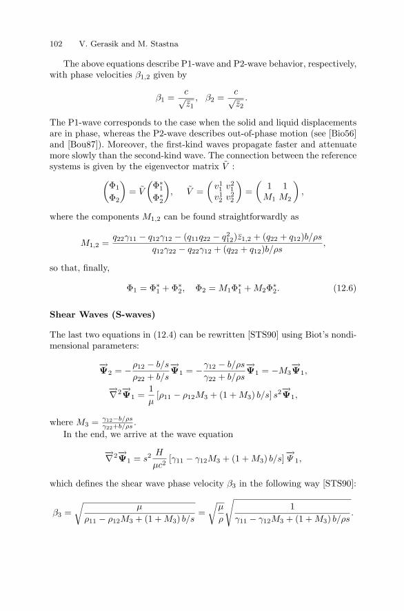
102 V. Gerasik and M. Stastna
The above equations describe P1-wave and P2-wave behavior, respectively,with phase velocities β1,2 given by
β1 =c√z1
, β2 =c√z2
.
The P1-wave corresponds to the case when the solid and liquid displacementsare in phase, whereas the P2-wave describes out-of-phase motion (see [Bio56]and [Bou87]). Moreover, the first-kind waves propagate faster and attenuatemore slowly than the second-kind wave. The connection between the referencesystems is given by the eigenvector matrix V :
(Φ1
Φ2
)= V
(Φ∗
1
Φ∗2
), V =
(v11 v2
1
v12 v2
2
)=
(1 1
M1 M2
),
where the components M1,2 can be found straightforwardly as
M1,2 =q22γ11 − q12γ12 − (q11q22 − q2
12)z1,2 + (q22 + q12)b/ρs
q12γ22 − q22γ12 + (q22 + q12)b/ρs,
so that, finally,
Φ1 = Φ∗1 + Φ∗
2, Φ2 = M1Φ∗1 + M2Φ
∗2. (12.6)
Shear Waves (S-waves)
The last two equations in (12.4) can be rewritten [STS90] using Biot’s nondi-mensional parameters:
−→Ψ2 = −ρ12 − b/s
ρ22 + b/s
−→Ψ1 = −γ12 − b/ρs
γ22 + b/ρs
−→Ψ1 = −M3
−→Ψ1,
−→∇2−→Ψ1 =1
µ[ρ11 − ρ12M3 + (1 + M3) b/s] s2−→Ψ1,
where M3 = γ12−b/ρsγ22+b/ρs .
In the end, we arrive at the wave equation
−→∇2−→Ψ1 = s2 H
µc2[γ11 − γ12M3 + (1 + M3) b/s]
−→Ψ 1,
which defines the shear wave phase velocity β3 in the following way [STS90]:
β3 =
õ
ρ11 − ρ12M3 + (1 + M3) b/s=
õ
ρ
√1
γ11 − γ12M3 + (1 + M3) b/ρs.

12 Dynamic Response of a Poroelastic Half-Space 103
12.3 General Solution of the 2D Problem
Consider a poroelastic half-space with an open boundary occupying the regionz < 0. At time t = 0, the porous half-space is subjected to an impulsiveexternal line traction −P (x)δ(t) at the surface (instantaneous compression).The boundary conditions for the governing equations (12.1),(12.2) and stress–strain relation can be represented in the form (z = 0)
σzz(x, 0, t) = −P (x)δ(t),
σxz(x, 0, t) = 0, (12.7)
p(x, 0, t) = 0.
For the 2D problem, the introduction of the four scalar potentials Φ1, Φ2
and Ψ1, Ψ2 (Ψ1 and Ψ2 are linearly dependent) is sufficient, so the 2D problemreduces to the solution of the wave equations in Laplace space:
β21∇2Φ∗
1 = s2Φ∗1, β
22∇2Φ∗
2 = s2Φ∗2, β
23∇2Ψ1 = s2Ψ1. (12.8)
Equations (12.8), written in Fourier space, become (here and below, trans-formed solutions will be indicated by the arguments)
∂2Φ∗1,2(k, z, s)
∂z2=
(k2 +
s2
β21,2
)Φ∗
1,2(k, z, s),∂2Ψ1(k, z, s)
∂z2=
(k2 +
s2
β23
)Ψ1.
Taking into account the far-field conditions (at infinity), the solutions of theabove wave equations can be expressed in the form
Φ∗1,2(k, z, s) = A1,2(k, s) exp [−z · ξ1,2(k, s)] ,
Ψ1(k, z, s) = B(k, s) exp [−z · ξ3(k, s)] ,(12.9)
where ξi(k, s) =√k2 + s2
β2i
(i = 1, 2, 3) and A1,2(k, s) and B(k, s) are unknown
coefficients to be determined from the boundary conditions (12.7).In the Laplace–Fourier space, the expressions for the stress tensor and the
pressure in terms of the potentials (12.8) can be written as
σzz(k, z, s) = (λ+ Y )[−k2Φ∗
1 − k2Φ∗2 + ξ2
1(k, s)Φ∗1 + ξ2
2(k, s)Φ∗2
]
−(R +Y )[k2M1Φ
∗1 + k2M2Φ
∗2 −M1ξ
21(k, s)Φ∗
1 −M2ξ22(k, s)Φ∗
2
]
+2µ[ξ21(k, s)Φ∗
1 + ξ22(k, s)Φ∗
2 + ikξ3(k, s)Ψ1
],
σxz(k, z, s) = µ(−2ikξ1(k, s)Φ
∗1 − 2ikξ2(k, s)Φ
∗2 + ξ2
3(k, s)Ψ1+ k2Ψ1
), (12.10)
p(k, z, s) = − 1
φY
[−k2Φ∗
1 − k2Φ∗2 + ξ2
1(k, s)Φ∗1 + ξ2
2(k, s)Φ∗2
]
− 1
φR
[−k2M1Φ
∗1 − k2M2Φ
∗2 +M1ξ
21(k, s)Φ∗
1 +M2ξ22(k, s)Φ∗
2
].
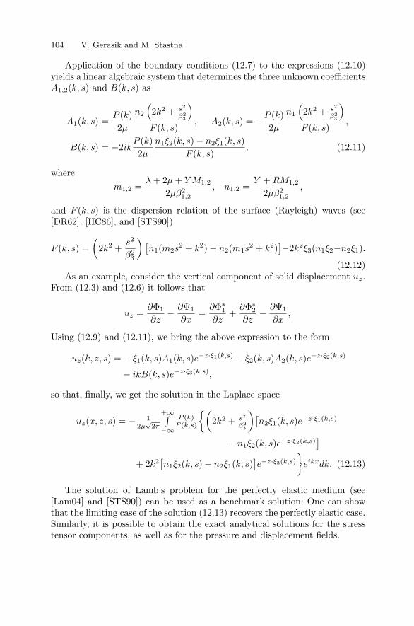
104 V. Gerasik and M. Stastna
Application of the boundary conditions (12.7) to the expressions (12.10)yields a linear algebraic system that determines the three unknown coefficientsA1,2(k, s) and B(k, s) as
A1(k, s) =P (k)
2µ
n2
(2k2 + s2
β23
)
F (k, s), A2(k, s) = −P (k)
2µ
n1
(2k2 + s2
β23
)
F (k, s),
B(k, s) = −2ikP (k)
2µ
n1ξ2(k, s) − n2ξ1(k, s)
F (k, s), (12.11)
where
m1,2 =λ + 2µ + Y M1,2
2µβ21,2
, n1,2 =Y + RM1,2
2µβ21,2
,
and F (k, s) is the dispersion relation of the surface (Rayleigh) waves (see[DR62], [HC86], and [STS90])
F (k, s) =
(2k2 +
s2
β23
) [n1(m2s
2 + k2) − n2(m1s2 + k2)
]−2k2ξ3(n1ξ2−n2ξ1).
(12.12)As an example, consider the vertical component of solid displacement uz.
From (12.3) and (12.6) it follows that
uz =∂Φ1
∂z− ∂Ψ1
∂x=
∂Φ∗1
∂z+
∂Φ∗2
∂z− ∂Ψ1
∂x,
Using (12.9) and (12.11), we bring the above expression to the form
uz(k, z, s) = − ξ1(k, s)A1(k, s)e−z·ξ1(k,s) − ξ2(k, s)A2(k, s)e−z·ξ2(k,s)
− ikB(k, s)e−z·ξ3(k,s),
so that, finally, we get the solution in the Laplace space
uz(x, z, s) = − 12µ
√2π
+∞∫−∞
P (k)F (k,s)
(2k2 + s2
β23
)[n2ξ1(k, s)e−z·ξ1(k,s)
− n1ξ2(k, s)e−z·ξ2(k,s)]
+ 2k2[n1ξ2(k, s) − n2ξ1(k, s)
]e−z·ξ3(k,s)
eikxdk. (12.13)
The solution of Lamb’s problem for the perfectly elastic medium (see[Lam04] and [STS90]) can be used as a benchmark solution: One can showthat the limiting case of the solution (12.13) recovers the perfectly elastic case.Similarly, it is possible to obtain the exact analytical solutions for the stresstensor components, as well as for the pressure and displacement fields.

12 Dynamic Response of a Poroelastic Half-Space 105
12.3.1 Harmonic Response
Despite the different form of the time dependence, it can be shown that the so-lution (12.13) can be used to describe the solution for a harmonic line source.In this particular case, we assume harmonic time-dependence for the dis-placements as well as for the components of the total stress tensor and porepressure. Thus, the first equation in (12.7) reads as σzz(x, 0, t) = −P (x)eiωt
and one gets, for example, the following expression for the normal solid-phasedisplacement at the surface (z = 0) in the physical domain:
uz(x, t,ω) =1
µ√
2πRe
⎧⎨⎩eiωt
+∞∫
−∞
P (k)ω2
β23
n2ξ1(k, ω) − n1ξ2(k, ω)
F (k, ω)eikxdk
⎫⎬⎭ ,
(12.14)
where ξi(k, ω) =√k2 − ω2
β2i
(i = 1, 2, 3) and F (k, ω) is obtained from the
Rayleigh wave secular equation F (k, s) (12.12) by the substitution s = iω.In the case of line traction, P (x) = Pδ(x), where P is a constant, so in
Fourier space we have P (k) = P√2π
(P has the dimensions of force per unit
length).The change of variable k = ωp
βSin (12.14), where
βS =
õ
ρ
√1
γ11 − γ212
γ22
,
and the introduction of the nondimensional quantities
x =ωx
βS, z =
ωz
βS, t = ωt, ω =
ρω
b=
ω
ωc, βi =
βS
βi(i = 1, 2, 3),
uz =4πµ
Puz, Uz =
4πµ
PUz, m1,2 = m1,2β
2S , n1,2 = n1,2β
2S ,
leads to expressions for the nondimensional vertical displacements in the form(from now on we omit the tilde)
uz(x, t, ω) = Re
+∞∫
−∞
β23
n2ξ1(p) − n1ξ2(p)
F (p, ω)ei(px+t)dp, (12.15)
Uz(x, t, ω) = −Re
+∞∫
−∞
1
F (p, ω) n2ξ1(p)
[2p2(M1 +M3) − β2
3M1
]−
−n1ξ2(p)[2p2(M2 +M3) − β2
3M2
] ei(px+t)dp, (12.16)
where ξi(p) =√p2 − β2
i (i = 1, 2, 3) and F (p, ω) is the nondimensionalizedsurface wave equation (12.12) [STS90]; that is,
F (p, ω) =(2p2 − β2
3
) [n1
(p2 −m2
)− n2(p
2 −m1)]− 2p2ξ3 (n1ξ2 − n2ξ1) .

106 V. Gerasik and M. Stastna
12.3.2 Numerical Example
Expressions (12.15) and (12.16) represent multivalued, slowly decaying, andhighly oscillating convergent integrals, so that special care is required in theirnumerical evaluation. Numerical results for the vertical solid and fluid dis-placements according to (12.15) and (12.16) are presented in Figures 12.1–12.3 for the poroelastic parameters of the Berea sandstone [CSD06] (see Table12.1). At the point x = 0, where the traction is applied, an integrable singu-larity can be observed; it can be shown that it will disappear in the case ofa uniformly distributed traction. The following frequencies are used in calcu-lations: ω = 0.1ωc, 1.0ωc, 10ωc, where ωc is the characteristic (or roll-over)frequency [Bio56] (see Table 12.1). Additional increase of the source frequencygives results similar to Figure 12.3.
x
0
0
5
555
10
1010 1515 2020
uz(x
,1,ω
),U
z(x
,1,ω
) solid phase uz
fluid phase Uz
Fig. 12.1. Normalized fluid and solid displacements. Source frequency ω = 0.1ωc.
x
0
0
5
555
10
1010 1515 2020
uz(x
,1,ω
),U
z(x
,1,ω
) solid phase uz
fluid phase Uz
Fig. 12.2. Normalized fluid and solid displacements. Source frequency ω = ωc.

12 Dynamic Response of a Poroelastic Half-Space 107
Table 12.1. Physical properties of the Berea sandstone and the saturating fluid(water).
Porosity φ 0.20Permeability (mD) k 360.0Tortuosity a 2.4Frame bulk modulus (GPa) Kb 10.37Shear modulus (GPa) µ 7.02Grain bulk modulus (GPa) Ks 36.5Liquid bulk modulus (GPa) Kf 2.25Solid density (kg m−3) ρs 2644.0Liquid density (kg m−3) ρf 1000.0Liquid viscosity (mPa s) ηf 1.0Characteristic frequency (kHz) ωc 48.0
x
0
0
5
555
10
1010 1515 2020
uz(x
,1,ω
),U
z(x
,1,ω
) solid phase uz
fluid phase Uz
Fig. 12.3. Normalized fluid and solid displacements. Source frequency ω = 10ωc.
12.4 Conclusions
Unlike in previous studies (for example, [VTZ95] and [HC86]), the main focusin this chapter is on the response at different source frequencies. Numerical re-sults demonstrate that the character of spatial oscillations is dependent on thesource frequency. For relatively low frequencies, displacements are observedto be in phase, with approximately the same amplitudes (see Figure 12.1).Increasing the source frequency leads to a weakening of the viscous couplingeffect, and as a consequence, solid and fluid displacements can be of differentamplitude and phase, or, in fact, nearly out of phase in the high-frequencyrange for certain materials. The numerical results are in agreement with Biot’sconclusion [Bio56] that when the characteristic frequency lies near unity (seeFigure 12.2), the inertia and viscous forces are approximately of the sameorder. Furthermore, our solution is in agreement with the results for solid-phase displacements and filtration amplitudes obtained in [VTZ95] by meansof separation of variables and the fast Fourier transformation. We have ex-tended our analysis to include the decomposition of the surface response into

108 V. Gerasik and M. Stastna
wave-train contour integrals for P1, P2, and S waves and a residue for theRayleigh wave response. In the far field, an asymptotic analysis analogous tothat in [Lam04] can subsequently be carried out. The results will be presentedelsewhere.
References
[Bio56] Biot, M.A.: The theory of propagation of elastic waves in a fluid-saturatedporous solid. J. Acous. Soc. Amer., 28, 168–191 (1956).
[Bou87] Bourbie, T., Coussy, O., Zinzner, B.: Acoustics of Porous Media. GulfPublishing Company, Paris (1987).
[CSD06] Chao, G., Smeulders, D.M.J., van Dongen, M.E.H.: Dispersive surfacewaves along partially saturated porous media. J. Acous. Soc. Amer., 119,1348–1355 (2006).
[deB05] de Boer, R.: Trends in Continuum Mechanics of Porous Media. Springer,Dordrecht (2005).
[DR62] Deresiewicz, H., Rice, J.T.: The effect of the boundaries on wave propa-gation in a liquid filed porous solid. Bull. Seism. Soc. Amer., 52, 627–638(1962).
[DD84] Dey, S., De, R.K.: Stresses in fluid-saturated porous half-space due to thenormal and tangential loadings. Indian J. Pure Appl. Math., 15, 1375–1397 (1984).
[FJ83] Feng, S., Johnson, D.L.: High-frequency acoustic properties of a fluid/porous solid interface. II. The 2D reflection Green’s function. J. Acous.Soc. Amer., 74, 915–924, (1983).
[HC86] Halpern, M., Christiano, P.: Response of poroelastic halfspace to steady-state harmonic surface tractions. Internat. J. Numer. Anal. Geomech., 6,609–632 (1986).
[Lam04] Lamb, H.: On the propagation of tremors over the surface of an elasticsolid. Phil. Trans. Roy. Soc. London, A203, 1–42 (1904).
[MLC05] Mesgouez, A., Lefeuve-Mesgouez, G., Chambarel, A.: Transient mechani-cal wave propagation in semi-infinite porous media using a finite elementapproach. Soil Dynamics Earth Engng., 25, 421–430 (2005).
[Mol02] Molotkov, L.A.: Sources acting on the free boundary of a porous Biotmedium and reflection on this boundary. J. Math. Sci., 5, 3750–3762(2002).
[Pau76] Paul, S.: On the displacements produced in a porous elastic half-spaceby an impulsive line load (no dissipative case). Pure Appl. Geophys., 4,605–614 (1976).
[Phi88] Philippacoupoulos, A.J.: Lamb’s problem for fluid saturated porous me-dia. Bull. Seism. Soc. Amer., 78, 908–923 (1988).
[STS90] Seimov, V.M., Trofimchuk, A.N., Savitsky, O.A.: Oscillations and Wavesin Layered Media. Naukova Dumka, Kiev (1990) (Russian).
[VTZ95] Valiappan, S., Tabatabaie, J., Zhao, C.: Analytical solution for two-dimensional dynamic consolidation in frequency domain. Internat. J. Nu-mer. Anal. Geomech., 19, 663–682 (1995).
[Wil96] Wilmanski, K.: Porous media at finite strains. The new model with thebalance equation for porosity. Arch. Mech., 4, 591–628 (1996).

13
Convexity Conditions and Uniqueness andRegularity of Equilibria in Nonlinear Elasticity
S.M. Haidar
Grand Valley State University, Allendale, MI, USA; [email protected]
13.1 Introduction: Formulation of the Problem
In this chapter, we consider a nonhomogeneous, isotropic, hyperelastic bodythat, in its reference configuration, occupies the open bounded subset Ω ofR
3 and has a stored-energy function
W : Ω × M3×3+ → [0,∞).
We assume W to be frame-indifferent and isotropic. That is, W satisfies,respectively [TN65],
W (x, RF ) = W (x, F ) and W (x, FR) = W (x, F )
for all x ∈ Ω, F ∈ M3×3+ , and R proper orthogonal. With W satisfying
additional plausible growth and convexity conditions, we aim to study theuniqueness and regularity of solutions to the equilibrium equations of nonlin-ear elasticity in which the boundary of the elastic body under considerationis subjected to homogeneous deformations. Our study is partly motivated bythe work of Ball [Bal82] and that of Knops and Stuart [KS84] regarding theuniqueness and regularity of solutions to the pure displacement boundaryvalue problem of nonlinear elastostatics.
In the absence of external forces, the total stored energy associated witha deformation u(·) of the body is given by
u → J(u, Ω) :=
∫
Ω
W (x,∇u(x))dx, (13.1)
and the equilibrium equations are given by the Euler–Lagrange equations
div
[∂W
∂F(x, F )
]= 0, x ∈ Ω,

110 S.M. Haidar
where F ≡ ∇u(x). For a given positive real number λ, we mainly1 considerthe questions of uniqueness and regularity of solutions of
div
[∂W
∂F(x, F )
]= 0 in Ω, (13.2)
u(x) = λx on ∂Ω. (13.3)
In what follows, we use the abbreviation (DBVP) to refer to the problemconsisting of equations (13.2) and (13.3). Generally, for the pure displace-ment boundary value problem of nonlinear elasticity, it is sufficient [AB78] toconsider only those deformations for which the condition
det[∇u(x)] > 0
holds for each x in Ω. Following the terminology in [Bal82] and [Ada75], wesay that u ∈ W 1,1(Ω; R3) is a weak solution of (DBVP) if
det(∇u(x)) > 0 for a.e. x ∈ Ω
∂W
∂F(·,∇u(·)) ∈ L′(Ω; R9), and
∫
Ω
∂W
∂ui,α
φi,αdx = 0 for all φ ∈ C∞
0 (Ω; R3).
In Section 13.2, the main section of this chapter, we present an answer to thequestion posed by Ball [Bal82] of whether strong ellipticity of W implies theexistence of nontrivial equilibrium solutions passing through the origin O andhaving finite energy. We also describe a class of stored-energy functions toshow that the uniqueness results of [Bal82] and [Hil57] do not carry over tothe nonhomogeneous case.
In the general theory of nonlinear elasticity, there are plenty of situationswhen uniqueness of solutions to the equilibrium equations of elasticity can-not be expected (see, for example, [Bal77a], [Hil57], [Joh72], and [TN65]).Of course, a stored-energy function W that is strictly convex in F ensuresuniqueness. Such a property, however, is completely unrealistic [TN65] as,among many other reasons, it violates the principle of frame-indifference. Theclass of admissible stored-energy functions has been modified to ensure tosome extent the existence, uniqueness, and regularity of solutions for someproblems of nonlinear elasticity (more details are given in [Bal77b], [BM84],[Eri83], [Mor52], and [Mor66]). This modification pertains to the generaliza-tion of the (traditional) notion of convexity to such concepts as polyconvexity(p.c.), quasiconvexity (q.c.), rank-one-convexity (r.1.c), etc. For homogeneousmaterials and in the case of the pure displacement boundary value problem,the first general uniqueness result that employs some of the above-mentioned(weaker) notions of convexity is due to [KS84]. We remark that this resultdoes not require W to be isotropic.1 Haidar [Hai00] presented a theorem of existence of energy-minimizing deforma-
tions for the variational problems associated with (13.2) and (13.3).

13 Convexity Conditions in Nonlinear Elasticity 111
Theorem 1 (Knops and Stuart [KS84]). Let Ω ⊂ R3 be an open bounded
domain that is star-shaped with respect to the point x0 ∈ Ω, and whose bound-ary ∂Ω is piecewise continuously differentiable. For any given F in M3×3
+ andc in R
3, let u and ψ be solutions of (13.2) with u(x) = ψ(x) = Fx + c forx ∈ ∂Ω, let W ∈ C2(M3×3
+ , R), and assume that W is rank-one-convex andstrictly quasiconvex at F . Then u(x) = ψ(x) = F (x) + c for all x ∈ Ω.
By restricting the geometrical structure of Ω to be the unit ball in R3, Ball
[Bal82] discussed conditions other than rank-one-convexity and quasiconvexityto ensure the uniqueness of homogeneous radial equilibria. In this case, theadmissible deformations are considered to be of the form
u(x) =r(R)
Rx, (13.4)
where R = |x|. Before we state Ball’s uniqueness result, let us recall thefollowing well-known representation theorem due to [RE55] (see, also, [TN65],pp. 28 and 317).
Theorem 2. W is isotropic and frame-indifferent if and only if there existsa function φ : Ωx(0,∞)3 → R such that φ(x, ·, ·, ·) is symmetric and
W (x, F ) = φ(x, v1, v2, v3), for all F ∈ M3×3+ ,
where the principal stretches v1, v2, v3 of F are the singular values of F .
For u ∈ W 1,1(Ω; R3), the weak derivatives of u in (13.4) are given by
∇u(x) =r(R)
R1 +
x ⊗ x
R2
[r′(R) − r(R)
R
], for a.e. x ∈ Ω. (13.5)
Equation (13.5) implies that
v1 = r′, v2 = v3 = r/R.
The total energy functional J(u;Ω) in (13.1) now becomes J(u;Ω) = 4πI(r),where
I(r) :=
∫ 1
0
R2φ(R; r′, r/R, r/R)dR. (13.6)
It is known ([Bal82], Theorem 4.2) that u(x) = (r/R)x ∈ W 1,1(Ω; R3) isa weak equilibrium solution if and only if r′(R) > 0 a.e. in (0, 1), R2φ,1 (R)
and R2φ,2 (R) ∈ L1(0, 1), and R2φ,1 (R) = 2
∫ R
1
ρφ,2 (ρ)dρ + const., a.e. in
(0, 1), where φ,i (R) = φ,i
(R; r′,
r(R)
R,r(R)
R
)for i = 1, 2.

112 S.M. Haidar
Theorem 3 (for homogeneous materials, Ball [Bal82]). Assume that(H1) φ ∈ C3((0,∞)3),(H2) φ satisfies the Baker–Ericksen inequalities
viφ,i −vjφ,jvi − vj
> 0, i = j, vi = vj , and φ,i = φ,i (v1, v2, v3); i, j = 1, 2, 3,
(H3)φ,1 (v1, v2, v2)
v22
→ −∞ as v1, v2 → 0+, with v1 > v2,
(H4)φ,1 (v1, v2, v2)
v22
→ +∞ as v1, v2 → +∞, with v1 < v2,
(H5) r ∈ C1(0, 1) is a solution of the equilibrium equations associated withI(r) with r′ > 0 for all R ∈ (0, 1] and r(0) = lim
R→0+r(R) = 0.
Then r(R) = λR, R ∈ [0, 1] for some λ > 0.
This result guarantees that the only radial equilibrium solutions withr(0) = 0 are the trivial ones. In that work, Ball argued that the growthhypotheses (H3) and (H4) are essential for every weak solution with r(0) = 0to be trivial (i.e., homogeneous) by giving an example showing that strongellipticity is not a sufficient condition for the uniqueness of such solutions. Heconsidered
W (F ) = φ(v1, v2) = g(η, δ) = ηaδ−b, (13.7)
where η = v1 + v2, δ = v1v2, and a, b ∈ R+, and showed the existence of
solutions of the form r(R) = λRγ for some positive real number γ = 1. Butthe total energy associated with such a solution is always infinite. Ball thenposed the following open question:
(BQ) “Does strong ellipticity imply that all solutions of the equilibrium equa-tions which pass through the origin and have finite energy are trivial?” (seeRemark 2.2).
13.2 Uniqueness and Regularity of Radial Equilibria
To effect an extreme deformation, that is, to compress the body to zero volumeor to expand it to infinite volume, we require an infinite amount of energy.This natural observation amounts to having the stored-energy function Wobey the following growth behavior2:
W (x, F ) → +∞ as detF → 0+ or + ∞. (13.8)
In terms of φ, (13.8) is equivalent to the following property:
2 Note that one cannot expect a convex function to be finite and yet exhibit thistype of singular behavior.

13 Convexity Conditions in Nonlinear Elasticity 113
limvi→0+
φ = limvi→+∞
φ = +∞, i = 1, 2, 3. (13.9)
From the preceding discussion we see that the smooth stored-energy functionφ must be chosen so that φ ≥ 0, φ(R; ·, ·, ·) is symmetric in v1, v2, and v3, andsatisfies properties (13.8) and (13.10).
Our first model shows that Theorem 1 and Theorem 3 do not carry overto the nonhomogeneous case. Indeed, let f(R, r, r′) denote the integrand ofI(r) in (13.10), namely,
f(R, r, r′) = R2φ
(R; r′,
r
R,
r
R
). (13.10)
For some γ ∈ (0, 1) and for every ε > 0, we assume that f satisfies theconstitutive property
f(εR, εγr, εγ−1r′) = ε−1f(R, r, r′). (13.11)
This homogeneity property was used by [BM85] to study the regularity ofminimizers for one-dimensional variational problems in the calculus of varia-tions. We have successfully applied it [Hai00] in modeling the onset of fracturein nonhomogeneous elastic materials where we presented, for the first time,a physical interpretation of this scale-invariance property (see Remark 2.2below). Setting ε = 1
R in (13.11) yields
f(R, r, r′) = R−1f(1, rR−γ , r′R1−γ). (13.12)
LetP (R, r′) = r′R1−γ and X(R, r) = rR−γ .
Relation (13.12) may now be rewritten as
f(R, r, r′) := R−1e(P, X), (13.13)
wheree(P, X) = f(1, X, P ).
Due to the symmetry property of φ(R; ·, ·, ·) in v1, v2, and v3, we observe thatφ(R; r′, r/R, r/R) is the restriction of φ(R; v1, v2, v3) to the plane v2 = v3 =r/R. Equivalently, e(P, X) is the restriction to the plane X1 = X2 = X ofthe symmetric quantity E(P, X1, X2) associated with φ(R; v1, v2, v3), whereXi = vi+1R
1−γ for i = 1, 2. Moreover, the condition φ,11 (R; r′, r/R, r/R) ≥ 0is equivalent to e,pp (P, X) ≥ 0.
For some λ ∈ (0,+∞), we observe that an r(·) of the form r(R) = λRγ
must be an absolute minimizer for I(·) in (13.10) because along such r(·) andin the light of (13.13), one has
I(r) =
∫ 1
0
R−1 c(λγ, λ)dR,

114 S.M. Haidar
which will yield the value zero only if there is a zero of c of the form (λγ, λ) inthe PX-plane. So an r(·) of the form r(R) = λRγ corresponds to a point alongthe line P = γX in the PX-plane or, equivalently, to an admissible solutionof the ordinary differential equation P = γX. We are now in a position topresent the first model. We must say that one generally would not expect thatsolutions in the nonhomogeneous case are trivial. Nevertheless, the interestingspecial feature of this model is to illustrate that (even) when W satisfiesfavorable constitutive hypotheses such as those given in Theorems 1 and 3,(DBVP) may still have nontrivial solutions.
Theorem 4 (Model 1). There exist positive numbers λ and C such that theequilibrium equations associated with the total energy functional I(r) for
e(P, X) := (PX2)5/3 −2(PX2)2/3 +(PX2)−1/3 +(P −C)2(X −C)4 (13.14)
admit nontrivial solutions of the form r(R) = λRγ , R ∈ [0, 1].
Proof. By direct computation, one can easily verify that e,pp > 0 for all P andX > 0. The function e satisfies the natural growth condition (13.9). From thediscussion that preceded the statement of this theorem, it is also clear thate is the restriction to the plane X1 = X2 = X of the symmetric function Egiven by
E(P, X1, X2)=(PX1X2 − 1)2(PX1X2)−1/3 + (P − C)2(X1−C)2(X2−C)2.
More importantly, e satisfies the hypotheses of the uniqueness Theorem 3 forthe following reason:
e,p = X2/3(PX2 − 1)(PX2)−4/3(5PX2 + 1) + 2(P − C)(X − C)4.
As P, X → 0+, e,p /X2 behaves like −(PX2)−4/3. Thus, e,p /X2 → −∞as P,X → 0+. On the other hand, as P, X → +∞, e,p /X2 behaves like53 (PX2)1/3. Hence, e,p /X2 → +∞ as P, X → +∞. We have, therefore,established the admissibility of e or, equivalently, that of φ. It remains forus to establish the existence of solutions of the form r(R) = λRγ for someλ ∈ (0,+∞).
Put X = t and P = γt. We want to show that for appropriate choices ofthe numbers λ and C, there exists t0 > 0 such that e(γt0, t0) = 0. By (13.14),
e(γt, t) = γt3 − 1)2(γt3)−1/3 + (γt − C)2(t − C)4.
It is not difficult to see that for t0 = λ = C = γ−1/3, one obtains e(γt0, t0) = 0.
That is, φ(R; r0(R), r0(R)R , r0(R)
R ) = 0, where
r0(R) = γ−1/3Rγ , R ∈ [0, 1]. (13.15)

13 Convexity Conditions in Nonlinear Elasticity 115
Remark 1. By considering the first three terms of e of (13.14), namely,
e(P, X) = (PX2 − 1)2(PX2)−1/3, (13.16)
one obtains a model that also satisfies the conditions of the uniqueness Theo-rem 1. Note that the stored-energy function W corresponding to e is polycon-vex as e is convex in the quantity PX2. On the other hand, it is clear that theunit ball Ω is star-shaped with respect to every point x0 ∈ Ω. However, foreach γ ∈ (0, 1), the equilibrium equation associated with e has a solution ofthe form given by (13.15). It is worth mentioning that, although e of (13.16)takes the value zero along the curve PX2 = 1, e vanishes at only one point ofthe PX-plane.
Theorem 4 with e as in (13.14) or (13.16) is easily seen to remain valid inthe case of n-dimensional elasticity.
Remark 2. Equation (13.7), which represents Ball’s example ([Bal82], p. 591),crucially depends on n, the number of elasticity dimensions. This dependenceis not so much in reference to the obvious difficulty of testing for the convexityof W , especially for n > 2, but rather to the conclusion of the example.According to Ball [Bal82], that example yields solutions of the form r(R) = Rα
with α > 0 if either α = 1 or
a ∈ [2b, 2(b + 1)], α = [a − 2(b + 1)]/(1 − 2b)(1 − b − 1). (13.17)
In n-dimensional elasticity with
φ(v1, . . . , vn) = (η)a(δ)−b,
one can simply verify by direct computation that the homogeneous deforma-tion r(R) = λR is an equilibrium solution if and only if n = 3 or a = nb.In terms of (13.17), this says that the case α = 1 is not possible, and conse-quently, the deformations r(R) = λR and r(R) = λRα with α > 0 and = 1do not coexist as solutions of the equilibrium equations of (13.7).
Our next result provides a strongly elliptic model in which both the trivialand nontrivial equilibria coexist. Furthermore, the energy associated with eachof these solutions is finite. In fact, a slight modification of this model yieldsan example of genuine nonuniqueness in which these different solutions havethe same finite energy. This homogeneous model, which is the main result ofthis chapter, represents an answer to (BQ). We now give the statement in thecase of plane elasticity.
Theorem 5 (Model 2-H). Let the positive odd integer a and the positivereal number b be given so that
1 + 2b ≤ a ≤ 2 + 2b. (13.18)
Then (i) the function φ given by

116 S.M. Haidar
φ(r′, r/R) = |r′ − r/R|a(r′r/R)−b (13.19)
is strongly elliptic, and (ii) the equilibrium equations associated with (13.19)have nontrivial solutions of the form r0(R) = λRγ , R ∈ [0, 1], with I(r) <+∞.
Proof. The proof of Theorem 5(i) is simply a verification by direct compu-tation of a set of conditions on φ, which were developed by [AT80] and areequivalent to the requirement that W be strongly elliptic (see [Hai89], Ch. 3).
The equilibrium equation associated with (13.19) is
d
dR
[R2 ∂φ
∂r′
]= R2 ∂φ
∂r
or, equivalently,
Rr′′φ,11 +(v1 − v2)φ,12 = φ,2 −2φ,1 , (13.20)
where φ,ij =∂φ,i∂vj
, i = 1, 2, v1 = r′, v2 =r
R.
Equation (13.20) has nontrivial weak solutions of the form r0(R) =λRγ , γ ∈ (0, 1), as long as a and b are chosen so that
a − 2b − 3(1 − γ)−1 < 0. (13.21)
However, this condition is automatically satisfied by hypothesis (13.18) of theabove theorem.
For example, taking a = 7, b = 3, and γ = (135±√
5553/132) gives rise toweak equilibrium solutions of the form r0(R) = λRγ . Furthermore, the energyassociated with such solutions is I(r0) = [3 − (1 − γ)(1 − 2b)]−1, which, by(13.21), is finite.
This model shows that strong ellipticity is not sufficient for solutions pass-ing through the origin and having (13.19), and constructs weak equilibriumsolutions of the form r(R) = λRγ having the same energy value as the trivialsolution. In n-dimensional elasticity, the above model still corresponds to anatural state and also yields nontrivial equilibrium solutions exactly like inthe case n = 2. The corresponding model (13.10) becomes
(n − 1)|r′ − r/R|a[r′(r/R)n−1]−b.
In the nonhomogeneous case, the answer to the analogous question to (BQ)is also negative as can be seen from Theorem 4 and the discussion leading to it.It is interesting to note that the nonhomogeneous version of model (refeqn:hai-19) by itself does not yield the same conclusion as above. More specifically,the function e given by
e(P, X) := |P − X|1(PX)−b (13.22)

13 Convexity Conditions in Nonlinear Elasticity 117
is strongly elliptic for 1 + b < a ≤ 2 + 2b. Moreover, the equilibrium equationassociated with (13.22), namely,
e,1 +R
[e,22
dP
dR+ e,12
dX
dR
]= e,2 ,
has nontrivial weak solutions of the form r0(R) = λRγ , γ ∈ (0, 1), as long asa = 2b. The value of the energy associated with such a solution, however, isalways infinite. While keeping it strongly elliptic, it is possible to modify e in(13.22) in such a way that the corresponding value of the energy associatedwith r0 is finite (in fact, equal to zero).
Additional results that supplement this work will be forthcoming in an-other paper to be submitted to J. Nonlinear Anal. They have to do with thefundamental question of regularity and with obtaining formulations of theproblem that are amenable to successful numerical treatments.
Acknowledgement. This work was partially supported by a grant from the office ofResearch and Development under Dean P. Kimboko, Grand Valley State University.
References
[Ada75] Adams, R.A.: Sobolev Spaces. Academic Press, New York (1975).[AB78] Antman, S.S., Brezis, H.: The existence of orientation-preserving deforma-
tions in nonlinear elasticity. In: Knops, R.J. (ed.), Nonlinear Analysis andMechanics, vol. II. Pitman, London (1978).
[AT80] Aubert, G., Tahroui, R.: Sur la faible fermeture des certains ensembles deconstraintes en elasticite nonlineaire plane. C.R. Acad. Sci. Paris Ser. I,290, 537–540 (1980).
[Bal77a] Ball, J.M.: Constitutive inequalities and existence theorems in nonlinearelastostatics. In: Knops, R.J. (ed.), Nonlinear Analysis and Mechanics, vol.I. Pitman, London, 187–241 (1977).
[Bal77b] Ball, J.M.: Convexity conditions and existence theorems in nonlinear elas-ticity. Arch. Rational Mech. Anal., 63, 337–403 (1977).
[Bal82] Ball, J.M.: Discontinuous equilibrium solutions and cavitation in nonlinearelasticity. Phil. Trans. Roy. Soc. London, 306, 557–611 (1982).
[BM84] Ball, J.M., Murat, F.: W 1,P -quasiconvexity and variational problems formultiple integrals. J. Functional Anal., 58, 225–253 (1984).
[BM85] Ball, J.M., Mizel, J.V.: One-dimensional variational problems whose min-imizers do not satisfy the Euler-Lagrange equation. Arch. Rational Mech.Anal., 90, 325–388 (1985).
[Eri83] Ericksen, J.L.: Ill-posed problems in thermoelasticity theory. In: Ball, J.M.(ed.), Systems of Nonlinear Partial Differential Equations, Reidel, Dor-drecht (1983).
[Hai00] Haidar, S.M.: Existence and regularity of weak solutions to the displace-ment boundary value problem of nonlinear elastostatics. In: Bertram, B.,Constanda, C., Struthers, A. (eds.), Integral Methods in Science and En-gineering. Chapman & Hall/CRC, Boca Raton, FL (2000), pp. 161–166.
118 S.M. Haidar
[Hai89] Haidar, S.M.: The Lavrentiev phenomenon in nonlinear elasticity. Ph.D.Thesis, Department of Mathematics, Carnegie-Mellon University, Pitts-burgh, PA (1989).
[Hil57] Hill, R.: On uniqueness and stability in the theory of finite elastic strains.J. Mech. Phys. Solids, 5, 229–241 (1957).
[Joh72] John, F.: Uniqueness of non-linear elastic equilibrium for prescribedboundary displacements and sufficiently small strains. Comm. Pure Appl.Math., 25, 617–634 (1972).
[KS84] Knops, R.J., Stuart, C.A.: Quasi-convexity and uniqueness of equilibriumsolutions in nonlinear elasticity. Arch. Rational Mech. Anal., 86, 223–249(1984).
[Mor52] Morrey, C.B.: Quasi-convexity and the lower semi-continuity of multipleintegrals. Pacific J. Math., 2, 25–53 (1952).
[Mor66] Morrey, C.B.: Multiple Integrals in the Calculus of Variations. Springer,Berlin (1966).
[RE55] Rivlin, R.S., Ericksen, J.L.: Stress–deformation relations for isotropic ma-terials. J. Rational Mech. Anal., 4, 323–425 (1955).
[TN65] Truesdell, C., Noll, W.: The nonlinear field theories of mechanics. In:Flugge, S. (ed.), Handbuch der Physik, vol. III/3. Springer, Berlin (1965).

14
The Mathematical Modeling of Syringomyelia
P.J. Harris1 and C. Hardwidge2
1 University of Brighton, UK; [email protected] Princess Royal Hospital, Haywards Heath, UK; [email protected]
14.1 Introduction
The work presented in this chapter is concerned with constructing a mathe-matical model of the medical condition syringomyelia. This condition is char-acterized by the formation of voids or cavities in the spinal cord. An MRIscan of a typical patient is shown in Figure 14.1, where the void in the cord isclearly visible. Although the condition is in its early stages, the patients maynot be aware of it, but as it worsens, they can progressively lose the feelingin one or more limbs and may ultimately become paralyzed in the affectedlimbs. Once a patient has the condition, it is often impossible to treat it, butthere are established surgical procedures that help with preventing the con-dition from getting worse. However, why these procedures are so successful isnot fully understood. It is hoped that by mathematically modeling what ishappening in the spine, it will be possible to get some insight into the physicalprocesses that lead to the formation and worsening of the voids in the spinalcord. In this study, we have devised a simple model of the spinal cord thatcan be solved using the finite element method. Our initial studies were witha simple linearly elastic model, but additional studies have been conductedwith a viscoelastic model that may prove to give a more realistic response ofbiologic-type materials under different levels of external loading.
14.2 Description of Syringomyelia
The mechanics of syringomyelia formation and development has been the sub-ject of considerable debate. One hypothesis is that the formation and growthof these voids in the spinal cord is primarily due to the forces that result fromthe changes in pressure in the fluid surrounding the spinal cord. It is knownthat changes in the abdominal pressure cause a compression of the spinal du-ral sac and its contents. In turn, this causes both an increase in the pressureof the spinal fluid and a flow of the fluid from the spine into the fluid-filled

120 P.J. Harris and C. Hardwidge
sac that surrounds the brain inside the skull. In most people, when the ab-dominal pressure relaxes and the spinal cord decompresses, the fluid can flowback from the skull into the spine and the pressure levels return to normal.However, in some people, who either have a malformation of the bones at theback of the skull or have had some traumatic damage to the spine, the fluidis prevented from flowing from the skull back into the spine, and so, whenthe abdominal pressure relaxes, the pressure in the spinal fluid drops belowits equilibrium level. In turn, this allows the spinal cord to expand, and if theresulting tensions in the spinal cord are large enough, then voids may form,or get worse if they are already there.
Fig. 14.1. An MRI scan of a patient with syringomyelia.
14.3 Mathematical Model
The geometry of the human spine can be essentially considered as a numberof concentric circular cylinders (see Figure 14.2). The innermost cylinder isthe spinal cord itself, which can be considered as an elastic or viscoelasticsolid. It is surrounded by a layer of cerebral-spinal fluid, which is essentiallywater. This layer, in turn, is surrounded by a relatively thin layer of softtissue containing the blood vessels and other elements that the spine needs.

14 The Modeling of Syringomyelia 121
Fig. 14.2. Vertical cross section of the spine.
This layer also acts as the seal that keeps the cerebral-spinal fluid in place.Finally, on the outside are the bones that make up the spine and can beconsidered as rigid. Whilst the spinal cord is not exactly a circular cylinder(it is not exactly circular in cross section, and the human spine is curved),this is a good approximation and means that the cord can be modeled usingan axisymmetric model that greatly simplifies the analysis and reduces thesize of the computer model needed to solve the problem.
The initial model proposed here will consider only the spinal cord itself,and assumes that the changes in the pressure in the fluid surrounding the cordare a known function of time. The principal causes of pressure changes in thefluid are the motion of various muscles in the lower abdomen and changesin blood pressure in the soft tissues due to the heart pulse. The changes inpressure due to either of these can be determined from experimental data.
The finite element method has become established as one of the mainmathematical tools for modeling the motion of a finite elastic structure. Dis-cretizing the equations of motion of an elastic body using the finite elementmethod yields a matrix equation of the form
Mu + Ku = f, (14.1)
where K and M are the stiffness and mass matrices, respectively, u is thevector of nodal displacements, f is the consistent load vector, and a super-posed dot denotes differentiation with respect to time. The derivation of (14.1)can be found in numerous textbooks, such as [OCZ91], and is not repeatedhere. Given suitable initial conditions, it is possible to integrate this equationthrough time.

122 P.J. Harris and C. Hardwidge
An alternative to the linear elastic model is the use of a viscoelastic model,as this type of model can give a more realistic response of a biologic materialto external forces. In the work presented here, a viscoelastic stress–strainrelationship of the form
σ(x, t) = Dε(x, t) −n∑
j=1
∫ t
0
φj
τjDe(s−t)/τjε(x, s) ds
is used, where σ(x, t) is the vector of the nonzero components of the stresstensor at the point x and time t, ε is the vector of the nonzero componentsof the strain tensor, and D is the linear stress–strain matrix. Applying thestandard finite element method using this stress–strain relationship leads to
∫
V
BTσ(x, t) dVx =
∫
V
BTDB dVx u(t)
−n∑
j=1
φj
τj
∫
V
BTDB dVx ×∫ t
0
e(s−t)/τju(s) ds
= Ku(t) −n∑
j=1
φj
τj
∫ t
0
e(s−t)/τjKu(s) ds,
and hence, the finite element equations are
Ku(t) −n∑
j=1
φj
τj
∫ t
0
e(s−t)/τjKu(s) ds+Mu(t) = f(t), (14.2)
where K and M are the usual elastic stiffness and mass matrices. The integralsappearing in (14.2) can now be evaluated using a quadrature rule of the form
∫ t
0
e(s−t)/τjf(s) ds =
∫ t
0
e−u/τjf(t− u) du ≈N∑
i=0
wjif(t− ih). (14.3)
We note that the integral in (14.2) can be truncated at an upper limitmax(t, t0) since for u > t0, e
−u/τj becomes small enough that its contributionto the integral can be neglected. By using the quadrature rule given in (14.3),we can write the finite element equations (14.2) as⎛⎝1 −
n∑
j=1
φj
τjwj0
⎞⎠Ku(t) +Mu(t) = f(t) +K
N∑
i=1
⎛⎝
n∑
j=1
φj
τjwjiu(t− ih)
⎞⎠ .
(14.4)The final finite element equation (14.4) can now be integrated through timeusing any suitable numerical scheme. Here the trapezium method has beenused since it is known to be neutrally stable for solving elasticity and relatedproblems [KEA89].
Once the nodal displacements have been computed, it is possible to com-pute the stresses in the cord. These will give an indication of where possiblefuture damage may occur.
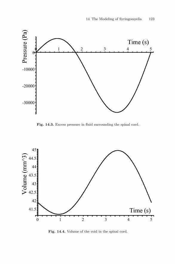
14 The Modeling of Syringomyelia 123
Fig. 14.3. Excess pressure in fluid surrounding the spinal cord.
Fig. 14.4. Volume of the void in the spinal cord.

124 P.J. Harris and C. Hardwidge
Fig. 14.5. Principal stress components in the spinal cord when the excess pressureis at its minimum.
Fig. 14.6. A comparison of the principal stresses in a solid cord and a cord with avoid when the excess pressure is at its minimum value.

14 The Modeling of Syringomyelia 125
14.4 Numerical Results
The results below are for computing the displacements in part of the spinalcord using a simple linearly elastic model. Typically, the human spinal cordis approximately 6 mm in radius, and the results are for a section of the cord60 mm long. The cord section considered here has a single ellipsoidal void ofradius 1 mm and length 10 mm located at the center of the cord. The mate-rial parameters for the spinal cord are Young’s modulus of 1.5 × 10⁶ N m−2,Poisson’s ratio of 0.49 (almost incompressible), and density 1500Kg m−3 (see[LEB96] for further details).
Figure 14.3 shows the pressure values in the fluid surrounding the spinalcord which are typical of the levels observed in a patient with syringomyelia.Figure 14.4 shows the corresponding volume of the void in the cord.
Figure 14.5 shows the principal stress components in the spinal cord whenthe excess pressure is at its lowest value. It can be seen that there are regionsof high tensile stresses around the ends of the hole, indicating that if damagewere to occur, then it is likely to be at the ends of the hole (i.e., the holewill get bigger). Furthermore, the results in Figure 14.6 show that tensilestresses occurring in a spinal cord that already has a void are greater thanthose occurring in a solid cord under the same loading. These results seemto indicate that the condition is more likely to get worse in a patient whoalready has the condition rather than developing in an unaffected patient.
14.5 Conclusions
The work presented in this chapter shows how to use the finite element methodto model the deformations of the human spinal cord due to the pressurechanges in the surrounding fluid. Furthermore, the results of this early workseem to support the hypothesis that it is the changes in the fluid pressurethat are responsible for development and/or worsening of syringomyelia in apatient. Future work will develop the model further, to include crack or voidformation and growth effects so that it should be possible to fully simulatewhat is happening in the spinal cord.
References
[KEA89] Atkinson, K.E.: An Introduction to Numerical Analysis, 2nd ed. Wiley,New York (1989).
[LEB96] Bilston, L.E., Thibault L.E.: The mechanical properties of the humancervical spinal cord in vitro. Biomed. Engng. Soc., 24, 67–74 (1996).
[OCZ91] Zienkiewicz, O.C., Taylor, R.L.: The Finite Element Method, vols. 1 and2. McGraw-Hill, London, (1991).


15
A System Iterative Method for SolvingFirst-Kind, Degraded Identity OperatorEquations
J. Hilgers1,2, B. Bertram1, and W. Reynolds2
1 Michigan Technological University, Houghton, MI, USA; [email protected],[email protected]
2 Signature Research Inc., Calumet, MI, USA;[email protected]
15.1 Introduction
A class of first-kind integral equations that arise, for example, in problems ofimage enhancement, feature kernels, or point spread functions (PSFs), whichare degraded versions of the Dirac delta function. Such PSFs depend on oneor more parameters whose value(s) derive from aperture size, incident wave-length, and sensor geometry.
In problems Kf = g of this type, with f the unknown object, the imageg and any approximate regularized solution fα are blurred forms of the samefunction f . It then makes sense to view fα as the image of a higher qualitysensor of similar type whose PSF has parameters altered to produce a narrowerwidth. This leads to the problem K2f = fα, which is approximately solved,thereby defining one system iteration.
In this chapter, this idea is introduced and a possible improvement isdemonstrated. The parameter-choice problem is more complicated and oc-curs in both directions. In the inverse direction, the parameter α controlsthe amount of regularization. In the forward direction, the PSF parameter(s)control PSF width, or sensor quality.
A class of first-kind integral equations of the form
∫ 1
0
KB(x − y)f(y)dy = g(y), 0 ≤ x ≤ 1, (15.1)
which arise in image enhancement, feature kernels, or PSFs, that are degraded,or smoothed, versions of the Dirac δ-function. Two examples are consideredin this chapter: a Gaussian kernel and a sinc kernel. Formulas and graphs ofthese are displayed in Section 15.2. A positive parameter controls the widthof the PSF. As B increases, the width of the PSF, and so the degree of image

128 J. Hilgers, B. Bertram, and W. Reynolds
blur, decreases. As B → ∞, KB → δ (in some sense), implying that the sensorbecomes perfect since (15.1) then is
g(x) =
∫ 1
0
δ(x− y)f(y)dy = f(x).
In problems of this type, the image g(x) and any regularized approximatesolution fα of (15.1) are both blurred forms of the object function f0(y). Thefunction fα is then viewed as the image of a higher quality sensor of similartype, meaning the same PSF with a larger value of B, B2 > B.
The new equation,KB2f = fα, (15.2)
is then approximately solved in an effort to obtain an improved reconstructionof the true object function f0(y).
To make this more precise, soppose that the PSF satisfies
(i) KB : L2 → L2 is completely continuous ∀B > 0,
(ii) ||KBf − f || → 0 as B → ∞ ∀f ∈ L2. (15.3)
The regularized solution to (15.1) will be taken as
fB,α = (K∗BKB + αL∗L)−1K∗
B g, (15.4)
where g = KBf0 + ǫ and ǫ is an additive noise vector. Equation (15.4) is theleast square solution to (15.1) with Tikhonov regularization applied. L is theregularization operator.
Then the algorithm represented by (15.2) is as follows:
(i) Input B, f0, g, L. Let R = g.
(ii) Compute fB,α via (15.4) (with g = R). Choose
α = αopt to minimize ||fB,α − f0||. (15.5)
(iii) Choose γ = C to minimize ||Kγf0 − fB,αopt ||.(iv) R ← fB,αopt , B ← C, go to (ii) (i.e., solve KCf = fB,αopt).
It is well known (see, for example, [Gro77], [HBR00], [HB04], [Mor84],[Tik63], and [TA77]) that (15.5) exists when
||ǫ||||g|| =
||ǫ||||KBf0||
< 1. (15.6)
Inequality (15.6) defines the condition for just the first iteration. Thereafter,(15.6) becomes
||ǫeff ||||KCf0||
< 1, (15.7)
where ǫeff is the effective error when the right-hand side R, which is initiallyǫ, is set to fB,αopt . Thus, R = KCf0 + ǫeff = fB,αopt so that
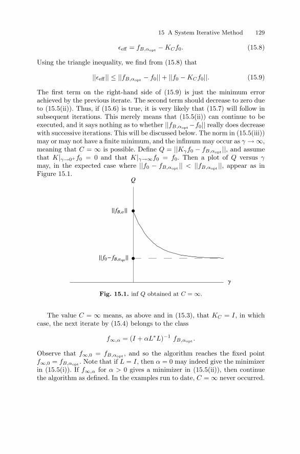
15 A System Iterative Method 129
ǫeff = fB,αopt − KCf0. (15.8)
Using the triangle inequality, we find from (15.8) that
||ǫeff || ≤ ||fB,αopt − f0|| + ||f0 − KCf0||. (15.9)
The first term on the right-hand side of (15.9) is just the minimum errorachieved by the previous iterate. The second term should decrease to zero dueto (15.5(ii)). Thus, if (15.6) is true, it is very likely that (15.7) will follow insubsequent iterations. This merely means that (15.5(ii)) can continue to beexecuted, and it says nothing as to whether ||fB,αopt −f0|| really does decreasewith successive iterations. This will be discussed below. The norm in (15.5(iii))may or may not have a finite minimum, and the infimum may occur as γ → ∞,meaning that C = ∞ is possible. Define Q = ||Kγf0 − fB,αopt ||, and assumethat K|γ→0+f0 = 0 and that K|γ→∞f0 = f0. Then a plot of Q versus γmay, in the expected case where ||f0 − fB,αopt || < ||fB,αopt ||, appear as inFigure 15.1.
Fig. 15.1. inf Q obtained at C = ∞.
The value C = ∞ means, as above and in (15.3), that KC = I, in whichcase, the next iterate by (15.4) belongs to the class
f∞,α = (I + αL∗L)−1 fB,αopt .
Observe that f∞,0 = fB,αopt , and so the algorithm reaches the fixed pointf∞,0 = fB,αopt . Note that if L = I, then α = 0 may indeed give the minimizerin (15.5(i)). If f∞,α for α > 0 gives a minimizer in (15.5(ii)), then continuethe algorithm as defined. In the examples run to date, C = ∞ never occurred.
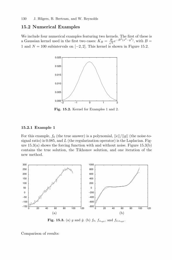
130 J. Hilgers, B. Bertram, and W. Reynolds
15.2 Numerical Examples
We include four numerical examples featuring two kernels. The first of these isa Gaussian kernel used in the first two cases: KB = B√
πe−B2(x2−y2), with B =
1 and N = 100 subintervals on [−2, 2]. This kernel is shown in Figure 15.2.
Fig. 15.2. Kernel for Examples 1 and 2.
15.2.1 Example 1
For this example, f0 (the true answer) is a polynomial, ||ǫ||/||g|| (the noise-to-signal ratio) is 0.085, and L (the regularization operator) is the Laplacian. Fig-ure 15.3(a) shows the forcing function with and without noise. Figure 15.3(b)contains the true solution, the Tikhonov solution, and one iteration of thenew method.
(a) (b)
Fig. 15.3. (a) g and g. (b) f0, fαopt , and f2,αopt .
Comparison of results:

15 A System Iterative Method 131
||fαopt − f0|| = 448 for αopt = 0.5,
||f2,αopt − f0|| = 315 for αopt = 8.0, B2 = 18.
The improvement is 30%.
15.2.2 Example 2
In this example, the Gaussian kernel is used, and the Laplacian is the regu-larizer. Here, the true solution f0 is two rectangles of different heights, andthe noise-to-signal ratio is ||ǫ||/||g|| = 0.068.
(a) (b)
Fig. 15.4. (a) g and g. (b) f0, fαopt , and f2,αopt .
Comparison of results:
||fαopt − f0|| = 7.79 for αopt = 0.8,
||f2,βopt − f0|| = 7.53 for βopt = 256.0, B2 = 18.
The improvement is 3.3%.The second kernel is the sinc kernel used in the last two cases:
KB =
sin B(x−y)
π(x−y) x = y,Bπ x = y,
with B = 1 and N = 100 subintervals on [−4, 4]. This kernel is shown inFigure 15.5.
15.2.3 Example 3
In this example, the sinc kernel is used, and the Laplacian is the regularizer.Here, the true solution f0 is two rectangles of different heights, and the noise-to-signal ratio is ||ǫ||/||g|| = 0.081.

132 J. Hilgers, B. Bertram, and W. Reynolds
Fig. 15.5. Kernel for Examples 3 and 4.
(a) (b)
Fig. 15.6. (a) g and g. (b) f0, αopt , and f2,αopt .
Comparison of results:
||fαopt − f0|| = 3.38 for αopt = 0.4,
||f2,βopt − f0|| = 3.28 for βopt = 2−8, B2 = 14.
The improvement is 3%.
15.2.4 Example 4
In this example, the sinc kernel is used, and the derivative operator is theregularizer. Here, the true solution f0 is a polynomial, and the noise-to-signalratio is ||ǫ||/||g|| = 0.019.
||fαopt − f0|| = 12864 for αopt = 4 × 10⁻³,
||f2,βopt − f0|| = 7982 for βopt = 2−6, B2 = 50.
The improvement is 38%.
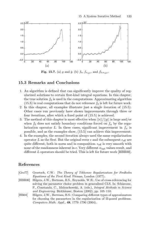
15 A System Iterative Method 133
(a) (b)
Fig. 15.7. (a) g and g. (b) f0, fαopt , and f2,αopt .
15.3 Remarks and Conclusions
1. An algorithm is defined that can significantly improve the quality of reg-ularized solutions to certain first-kind integral equations. In this chapter,the true solution f0 is used in the computations. Approximating algorithm(15.5) in real computations that do not reference f0 is left for future work.
2. In this chapter, all examples illustrate just a single iteration of (15.5).Other cases run previously have shown improvements through three orfour iterations, after which a fixed point of (15.5) is achieved.
3. The method of this chapter is most effective when ||ǫ||/||g|| is large and/orwhen f0 does not satisfy boundary conditions forced on fα by the regu-larization operator L. In these cases, significant improvement in fα ispossible, and as the examples show, (15.5) can achieve this improvement.
4. In the examples, the second iteration always used the same regularizationoperator L as the first. But the original error ǫ and the subsequent ǫeff arequite different, both in norm and in composition. ǫeff is very smooth withnone of the randomness inherent in ǫ. Very different αopt values result, anddifferent L operators should be tried. This is left for future work [HBR00].
References
[Gro77] Groetsch, C.W.: The Theory of Tikhonov Regularization for FredholmEquations of the First Kind. Pitman, London (1977).
[HBR00] Hilgers, J.W., Bertram, B.S., Reynolds, W.R.: Use of cross-referencing forsolving the parameter choice problem in generalized CLS. In: Schiavone,P., Constanda, C., Midouchowski, A. (eds.), Integral Methods in Scienceand Engineering. Birkhauser, Boston (2002), pp. 105–110.
[HB04] Hilgers, J.W., Bertram, B.S.: Comparing different types of approximatorsfor choosing the parameters in the regularization of ill-posed problems.Computers Math. Appl., 48, 1779–1790 (2004).

134 J. Hilgers, B. Bertram, and W. Reynolds
[Mor84] Morozov, V.A.: Methods for Solving Incorrectly Posed Problems. Springer,Berlin-Heidelberg-New York (1984).
[Tik63] Tikhonov, A.N.: Solution of incorrectly formulated problems and the reg-ularization method. Soviet Math. Dokl. (1963), pp. 1035–1038.
[TA77] Tikhonov, A.N., Arsenin, V.Y.: Solutions of Ill-Posed Problems. Winston,Washington, DC (1977).

16
Fast Numerical Integration Method UsingTaylor Series
H. Hirayama
Kanagawa Institute of Technology, Japan; [email protected]
16.1 Introduction
We consider the following integral over the finite range [a,b]:
I =
∫ b
a
f(x)dx,
where f(x) is a given smooth function.The arithmetic operations and functions of Taylor series can be defined
in Fortran 90, C++ [ES90], and C# programming languages. In addition,functions that consist of arithmetic operations, predefined functions, and con-ditional statements can quickly be expanded in Taylor series.
Using this procedure, we can expand f(x) at x = c as follows:
f(x) = f0 + f1(x − c) + f2(x − c)2 + f3(x − c)3 + · · · + fn(x − c)n. (16.1)
If we integrate the Taylor series in (16.1), that is,
F (x) = f0(x − c) +f1
2(x − c)2 +
f2
3(x − c)3 + · · · + fn
n + 1(x − c)n+1, (16.2)
then the integral over the interval [a,b] near x = c may be evaluated using(16.2).
The method outlined above provides us with an effective and fast numericalintegration technique.
16.2 Arithmetic of Taylor Series
In this section, we briefly explain the basic idea of how to expand functionsinto Taylor series. The reader is referred to Rall [Ral81], Henrici [Hen74], andHirayama [Hir02] for more details.

136 H. Hirayama
The arithmetic program for Taylor series can be developed without anydifficulty. The following relations are valid not only at the origin but also atany point of the interval [a,b]. The series can be defined in the form
f(x) = f0 + f1x + f2x2 + f3x
3 + f4x4 + · · · , (16.3)
g(x) = g0 + g1x + g2x2 + g3x
3 + g4x4 + · · · , (16.4)
h(x) = h0 + h1x + h2x2 + h3x
3 + h4x4 + · · · (16.5)
and possess the following important properties.
(i) Addition and subtraction. If h(x) = f(x) ± g(x), then the coefficientsof f , g, and h satisfy
hi = fi ± gi.
(ii) Multiplication. If h(x) = f(x)g(x), then the coefficients of f , g, and hsatisfy
hn =
n∑
k=0
fign−i.
(iii) Division. If h(x) = f(x)/g(x), then the coefficients of f , g, and hsatisfy
h0 =f0
g0, hn =
1
g0
(fn −
n−1∑
k=0
hkgn−k
), (n ≥ 1).
(iv) Exponential function. If h(x) = ef(x), then dh/dx = hdf/dx. Substi-tuting (16.3)–(16.5) into this differential equation and comparing the coeffi-cients of the Taylor series, we arrive at the relations
h0 = ef0 , hn =1
n
n∑
k=1
khn−kfk, (n ≥ 1).
We can get similar differential equations and similar relations betweenthe coefficients of the Taylor series for any other elementary transcendentalfunction.
16.3 Numerical Integration Method
In this section, we explain a numerical integration method using Taylor series.We consider the following integral over a finite interval [a, b]:
I =
∫ b
a
f(x)dx, (16.6)
where f(x) is a given smooth function. We expand the function f(x) at x = cin a Taylor series as

16 Fast Numerical Integration Method 137
f(x) = f0 + f1(x − c) + f2(x − c)2 + f3(x − c)3 + · · · + fn(x − c)n. (16.7)
The indefinite integral F (x) can be obtained by integrating the Taylor seriesderived in (16.7) as
F (x) = f0(x − c) +f1
2(x − c)2 +
f2
3(x − c)3 + · · · + fn
n + 1(x − c)n+1. (16.8)
If F (x) obtained in (16.8) converges sufficiently fast, then we can obtain thevalue of the integral by computing F (b) − F (a). If this is not the case, thenwe introduce the function h = x − c and from (16.8) we have
F (c + h) = f0h +f1
2h2 +
f2
3h3 + · · · +
fn
n + 1hn+1. (16.9)
Letting h be sufficiently small, the series in (16.9) becomes a fast convergentTaylor series.
The function h should be chosen so that the absolute value of the last termin (16.9) is less than the error ǫ of computation; i.e.,
∣∣∣∣fn
n + 1hn+1
∣∣∣∣ ≤ ǫ. (16.10)
From (16.10) we have
h ≤ n+1
√(n + 1)ǫ
|fn| . (16.11)
If h satisfies inequality (16.11), we can compute the numerical value of theintegral with error ǫ in the interval [c − h, c + h]. As the degree of the Taylorseries increases, the error of the computation tends to zero.
The numerical integral method described above can be summarized asfollows.
(i) Expand f(x) at the center c of the interval [a, b] into a Taylor series.(ii) Integrate the series.(iii) Compute h using (16.10) and divide the integral (16.6) into three
integrals:
∫ b
a
f(x)dx =
∫ c−h
a
f(x)dx +
∫ c+h
c−h
f(x)dx +
∫ b
c+h
f(x)dx.
(iv) The integral over [c − h, c + h] can be computed using the Taylorseries. The other integrals can be computed using this integration methodrecursively.
16.4 Numerical Example
Let us consider a numerical example.
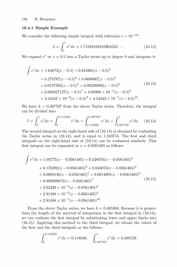
138 H. Hirayama
16.4.1 Simple Example
We consider the following simple integral with tolerance ǫ = 10−10:
I =
∫ 1
0
exdx = 1.71828182845904523 · · · . (16.12)
We expand ex at x = 0.5 into a Taylor series up to degree 9 and integrate it:
∫exdx = 1.64872(x − 0.5) + 0.824361(x − 0.5)2
+ 0.274787(x − 0.5)3 + 0.0686967(x − 0.5)4
+ 0.0137393(x − 0.5)5 + 0.00228989(x − 0.5)6
+ 0.000327127(x − 0.5)7 + 4.08909 × 10⁻⁵(x − 0.5)8
+ 4.54343 × 10⁻⁶(x − 0.5)9 + 4.54343 × 10⁻⁷(x − 0.5)10.
(16.13)
We have h = 0.387707 from the above Taylor series. Therefore, the integralcan be divided into
I =
∫ 1
0
exdx =
∫ 0.112293
0
exdx +
∫ 0.887707
0.112293
exdx +
∫ 1
0.887707
exdx. (16.14)
The second integral on the right-hand side of (16.14) is obtained by evaluatingthe Taylor series in (16.13), and is equal to 1.310713. The first and thirdintegrals on the right-hand side of (16.14) can be evaluated similarly. Thisfirst integral can be expanded at x = 0.0561465 as follows:
∫exdx = 1.05775(x − 0.0561465) + 0.528876(x − 0.0561465)2
+ 0.176292(x − 0.0561465)3 + 0.044073(x − 0.0561465)4
+ 0.0088146(x − 0.0561465)5 + 0.0014691(x − 0.0561465)6
+ 0.000209872(x − 0.0561465)7
+ 2.62339 × 10⁻⁵(x − 0.0561465)8
+ 2.91488 × 10⁻⁶(x − 0.0561465)9
+ 2.91488 × 10⁻⁷(x − 0.0561465)10.
(16.15)
From the above Taylor series, we have h = 0.405304. Because h is greaterthan the length of the interval of integration in the first integral in (16.14),we can evaluate the first integral by substituting lower and upper limits into(16.15). Applying this method to the third integral, we obtain the values ofthe first and the third integrals as the follows:
∫ 0.112293
0
exdx = 0.118840,
∫ 1
0.887707
exdx = 0.288729.

16 Fast Numerical Integration Method 139
Evaluating the right-hand side of (16.15) gives
I =
∫ 1
0
exdx = 1.718281828456585.
The first 12 digits of this result agree with the exact value in (16.12). If we usea Taylor series of order higher than 13, we can compute this integral withouta split of the interval of integration.
16.4.2 Kahaner’s Test Problems
Kahaner-type test problems [HH03] are usually considered to illustrate theeffectiveness of a computational method. These problems deal with discontin-uous and singular functions, but in this chapter, we use a slightly differentapproach to validate our method.
In this work, the calculation times of the numerical integration using Tay-lor series and AQE11D are compared. The integral routine AQE11D is codedbased on the eleventh order adaptive Newton–Cotes method [EU96], which isone of the fastest numerical integration routines.
The comparison performance on a Pentium 4 2.0 GHz is shown in Table16.1.
Table 16.1. Comparison of performance on Pentium 4 2.0 GHz of the quadratureroutine based on Taylor series with error tolerance 1.0E-09.
No. a b Integrand Taylor AQE11D Ratioµs µs
1 0.0 1.0 ex 1.02 3.06 3.404 -1.0 1.0 0.92 cosh x − cos x 3.52 7.50 2.405 -1.0 1.0 1/(x4 + x2 + 0.9) 5.70 8.54 1.708 0.0 1.0 1/(x4 + 1) 4.57 6.25 1.509 0.0 1.0 2/(2 + sin 3.14159x) 99.60 86.70 0.98
10 0.0 1.0 1/(1 + x) 1.60 3.12 2.2011 0.0 1.0 1/(ex + 1) 1.77 4.23 2.7012 0.0 1.0 1/(ex − 1) 1.44 7.53 5.9013 0.0 1.0 sin(314.1592x)/(3.141592x) 185.81 255.00 1.60
14 0.0 10.0√
(50)e503.14159x2
656.20 59.60 0.0915 0.0 10.0 25e−25x 63.90 26.20 0.4716 0.0 10.0 50/(3.14159(2500x2 + 1)) 23.24 29.80 1.40
17 0.01 1.0 sin(503.14159x)/(50(503.14159x)2) 103.751 227.00 2.4018 0.0 π cos(cos x + 3 sin x + 2 cos 2x
+ 3 sin 2x + 3 cos 3x) 156.08 81.80 2.4020 0.0 -1.0 1/(x2 + 1.005) 2.38 9.06 4.3021 0.0 1.0 1
cosh2(10(x−0.2))+ 1
cosh4(100(x−0.4))
+ 1cosh6(1000(x−0.6))
11927.20 - N/A

140 H. Hirayama
It may be observed from Table 1 that the method introduced in this chap-ter gives better results than AQE11D for many test problems, except forthe case when the integrated function decays rapidly or oscillates at highfrequency. Lower-order Taylor series cannot give a good approximation forrapidly decaying functions over a wide range because, by (16.11), the error ofintegration in this case is large. For such functions, a polynomial bounded atboth ends of the interval gives a better approximation than the Taylor seriesmethod.
16.5 Conclusion
The numerical integration method based on Taylor series is one of the fastestfor most functions. However, this method does not give good results for rapidlydecaying and high-frequency oscillating functions. The method can easily beapplied using the C++, C#, or Fortran 90 programming languages.
This method can also be applied, with slight modifications, to the integra-tion of singular and discontinuous functions.
References
[ES90] Ellis, M.A., Stroustrup, B.: The Annotated C++ Reference Manual.Addison-Wesley, New York (1990).
[EU96] Engeln-Mullges, G., Uhlig, F.: Numerical Algorithms with C. Springer,Berlin-Heidelberg-New York (1996).
[Hen74] Henrici, P.: Applied Computational Complex Analysis, vol. 1. Wiley, NewYork (1974).
[HH03] Hibino, S., Hasegawa, T., Ninomiya, I., Hosoda, Y., Sato, Y.: A doublyadaptive quadrature method based on the combination of the Ninomiyaand the FLR schemes. Trans. IPSJ, 44, 2419–2427 (2003) (Japanese).
[Hir02] Hirayama, H.: Numerical method for solving ordinary differential equationby Picard’s method. In: Schiavone, P., Constanda, C., Mioduchowski, A.(eds.), Integral Methods in Science and Engineering. Birkhauser, Boston(2002) pp. 111–116.
[Ral81] Rall, L.B.: Automatic Differentiation-Technique and Applications. Sprin-ger, Berlin-Heidelberg-New York (1981).

17
Boundary Integral Solution of theTwo-Dimensional Fractional Diffusion Equation
J. Kemppainen and K. Ruotsalainen
University of Oulu, Finland; [email protected], [email protected]
17.1 Introduction
In this chapter, we discuss the boundary integral solution of the fractionaldiffusion equation
∂α
tΦ − ∆Φ = 0 in QT = Ω × (0, T ),
B(Φ) = g on ΣT = Ω × (0, T ), (17.1)
Φ(x, 0) = 0 x ∈ Ω,
where the boundary operator B(Φ) = ΦΣTand ∂α
tis the Caputo time deriva-
tive of the fractional order 0 < α ≤ 1. For α = 1, we get the ordinary diffusionequation, and for α = 0, we have the Helmholtz equation.
Hilbert space methods to study the initial boundary value problems arewell known for the heat and wave equations (see [LM721] and [LM722]).
The boundary integral equation method for elliptic, parabolic, and hyber-bolic equations has been extensively studied by several authors (see [Cos92]and the references therein). The idea to represent the solution of these equa-tions as boundary potentials has been used for decades (centuries). Thismethod converts the problem to an equivalent integral equation on the bound-ary of the domain. The method has been well studied, for example, in [Cos92],[Cos04], and [HS89]. The functional framework has been the interpretation ofthe boundary integral operators as anisotropic pseudodifferential operatorsacting on anisotropic Sobolev spaces[Cos01]. In this way, the boundary inte-gral method is closely connected with the Hilbert space approach to the initialboundary value problems studied in [LM721] and [LM722].
In this chapter, we construct a fundamental solution by means of the FoxH-functions and represent the solution of (17.1) as a single-layer potential.Using the jump relations of the potential, we derive the appropriate bound-ary integral operator and compute its principal symbol. By analyzing theproperties of the principal symbol, we can then give the detailed mappingproperties of the single-layer operator in anisotropic Sobolev spaces, which

142 J. Kemppainen and K. Ruotsalainen
yield the unique solvability of the boundary integral equation, and thus, alsothe unique solvability of the initial-boundary value problem.
17.2 Boundary Integral Formulation of the Problem
17.2.1 The Fundamental Solution
The fundamental solution E(x, t) of the fractional diffusion equation is con-structed by taking the Laplace transform in the time variable and the Fouriertransform in the spatial variable of the fractional diffusion equation
(∂αt − ∆)E(x, t) = δ(x, t),
where δ(x, t) is the Dirac delta distribution. The transformed equation is then
(|ξ|2 + sα) E(ξ, s) = 1,
where the two-dimensional Fourier transform is defined by
u(ξ, t) =
∫
R2
e−i〈x,ξ〉u(x, t)dx
and the Laplace transform by
u(x, s) =
∫ ∞
0
e−stu(x, t)dt.
Hence, the Fourier–Laplace transform of the fundamental solution is
E(ξ, s) =1
|ξ|2 + sα.
Using the Laplace transform of the Mittag–Leffler functions [KS04]
∫ ∞
0
e−sttµk+β−1E(k)µ,β(−atµ)dt =
k!sµ−β
a+ sµ,
we find out that the Fourier transform of the fundamental solution is
E(ξ, t) = F(E)(ξ, t) = tαE(0)α,α(−|ξ|2tα).
By computing the inverse Fourier transform of the Mittag–Leffler function,we notice that the fundamental solution is the Fox H-function (see [KS04] and[PBM90])
E(x, t) = tα−1|x|−2H2012 (|x|2t−α|α,α
(1,1),(1,1)).
For later use, we need to compute the Laplace transform of the fundamen-tal solution. We have

17 Fractional Diffusion Equation 143
E(x, s) =
∫ ∞
0
e−stE(x, t)dt =1
2π
∫
R2
ei〈ξ,x〉 1
|ξ|2 + sαdξ.
Since the Fourier–Laplace transform of the fundamental solution is radial, i.e.,E(ξ, t) = E(|ξ|, t), its inverse transform is radial as well:
E(x, s) = E(|x|, s).
On the other hand, the Fourier transform of E(|x|, s) can be written as
E(ξ, s) =
∫ ∞
0
r[ ∫ π
−π
e−ir|ξ| cos(φ)dφ]E(r, s)dr = 2π
∫ ∞
0
rJ0(r|ξ|)E(r, s)dr,
by changing integration to polar coordinates. Now, by formula 6.576 (7) in[GR96] for the Bessel functions, we have
∫ ∞
0
rJ0(|ξ|r)K0(sα2 r)dr =
1
|ξ|2 + sα, Re(s) > 0.
Hence, the Laplace transform of the fundamental solution E(x, t) is
E(x, s) = 2πK0(|x|sα2 ). (17.2)
17.2.2 The Boundary Integral Equation
We now define the boundary potential
Φ(x, t) = Sσ(x, t) =
∫
Γ
∫ t
0
σ(y, τ)E(x− y, t− τ)dsydτ, x ∈ Ω, t ∈ (0, T )
for a given boundary distribution σ(x, t) ∈ C∞(ΣT ). The potential is the solu-tion of the fractional diffusion equation both in the interior domain Ω× (0, T )and in the exterior domain [Rn \ Ω] × (0, T ), with the zero initial condition.We denote the direct value of Sσ on the boundary by V σ.
The single-layer potential Sσ(x, t) is continuous up to the boundary dueto the asymptotic properties of the fundamental solution. This leads to theboundary relation
γ(Sσ) = γ(Φ) = V σ(x, t),
where γ : u → u|Γ is the trace operator. In other words, we have convertedthe initial-boundary value problem for the fractional diffusion equation (17.1)to the boundary integral equation
V σ(x, t) = γ(Φ)(x, t) = g(x, t), (x, t) ∈ ΣT .
Furthermore, the normal derivative of the single-layer potential experi-ences a jump across the boundary [KR]:
[∂nSσ]ΣT= σ.

144 J. Kemppainen and K. Ruotsalainen
17.3 Function Spaces
Let s ∈ R and m ≥ 1. The anisotropic Sobolev space Hsm(Rn+1) contains
those distributions u ∈ S′(Rn+1) for which the norm
‖u‖s,m = (2π)− n+12
( ∫
Rn+1
[(1 + |ξ|2)m + |η|2] sm |u(ξ, η)|2dξdη
) 12
is finite [Cos01]. Here the length of the vector ξ = (ξ1, ξ2, . . . , ξn) is denotedas usual by |ξ|2 = ξ2
1 + ξ22 + · · · + ξ2
n.Anisotropic Sobolev spaces on the cylinder T
n ×R are defined in the sameway as the anisotropic Sobolev spaces on R
n+1:
‖u‖s,m = (2π)− n2
( ∑
k∈Zn
∫
Rη
((1 + |2πk|2)m + |η|2
) sm |u(k, η)|2dη
) 12
Here u(k, η) for (k, η) ∈ Zn × R are defined as the Fourier coefficients in the
space variables and the Fourier transform in the time variable, i.e.,
u(k, η) =
∫
[0,1]n
∫
R
e−i(2π(k,x)+tη)u(x, t)dx dt,
with the scalar product (k, x) =∑n
l=1 klxl.
Finally, let us introduce the anisotropic Sobolev space Hsm(Rn+1), which
takes the vanishing initial condition at t = 0 into account; that is,
Hsm(Rn+1) = u ∈ Hs
m(Rn+1 : supp(u) ⊂ Rx × [0,∞[.
For a finite time-interval, we write Rn+1T = R
nx × (0, T ), T > 0, and set
Hsm(Rn+1
T ) = u = U |Rnx×(−∞,T ) : U ∈ Hs
m(Rn+1),
equipped with the norm
‖u‖s,m;T = inf‖U‖s,m : u = U |Rnx×(−∞,T ).
As above, we define Hsm(Tn × R) as the space of functions vanishing on
the negative time-axis and Hsm(ΣT ) as the space of the restrictions to ΣT =
Γ × (0, T ).
17.4 The Mapping Properties
In this section, we present the main results concerning the mapping propertiesof the single-layer operator
VΓuΓ (x, t) =
∫
Γ
∫ T
0
E(x− y, t− τ)u(y, τ)dsydτ.

17 Fractional Diffusion Equation 145
Since, by our assumption, the boundary curve Γ has a smooth parametricrepresentation θ → x(θ), we may identify every boundary distribution withthe 1-periodic distribution in the space variable u(θ, t) = uΓ (x(θ), t). Hence,the single-layer operator can be written as
V u(θ, t) =
∫ t
0
∫ 1
0
E(x(θ) − x(φ), t − τ)u(φ, τ)dφdτ. (17.3)
We will see from the properties of the fundamental solution that the single-layer operator is of Volterra type [KR]; i.e., if u(θ, τ) = 0 for τ < t, thenV u(θ, τ) = 0.
We will consider the single-layer operator as an anisotropic pseudodiffer-ential operator, and compute its principal symbol, whose properties yield themapping properties in the anisotropic Sobolev spaces defined above.
Applying the Laplace transformation and using (17.2), we get
L(V u)(x, s) =1
2π
∫ 1
0
u(φ, s)K0(|x(θ) − x(φ)|sα2 )|x′(φ)|dφ.
Since we assumed that u(φ, t) = 0, t < 0, we obtain the Fourier transform byputting s = iη:
V u(θ, η) =1
2π
∫ 1
0
u(φ, η)K0(|x(θ) − x(φ)|(iη)α2 )|x′(φ)|dη.
We define the function κ(θ, φ) by setting
κ(θ, φ) =|x(θ) − x(φ)|
2 sin(π(θ − φ)).
Hence, the kernel of the integral operator V can be written as
K0(|x(θ) − x(φ)|(iη)α2 ) = K0(2κ(θ, φ)(iη)
α2 sin(θ − φ)),
which is 1-periodic in θ−φ and has the Fourier series representation ([Obe73],(4.32))
K0(|x(θ) − x(φ)|(iη)α2 ) =
∑
p∈Z
I|p|(κ(θ, φ)(iη)α2 )K|p|(κ(θ, φ)(iη)
α2 )e2πpi(θ−φ).
Replacing the kernel of the single-layer operator by the Fourier series, weobtain the following representation of the operator:
V u(θ, t) =1
2π
∑
p∈Z
∫ 1
0
∫
Rη
a(θ, φ, p, η)u(φ, η)e2πpi(θ−φ)+iηtdφdη,
where the amplitude of the pseudodifferential operator is

146 J. Kemppainen and K. Ruotsalainen
a(θ, φ, p, η) =1
2πI|p|(κ(θ, φ)(iη)
α2 )K|p|(κ(θ, φ)(iη)
α2 )|x′(φ)|.
As in [Cos01] (Theorems 3.4 and 4.3), from the asymptotic expansion of theamplitude we now get the leading term by inserting φ = θ:
a(θ, p, η) = a(θ, θ, p, η) =1
2πI|p|(κ(θ)(iη)
α2 )K|p|(κ(θ)(iη)
α2 )|x′(θ)|,
where κ(θ) = |x′(θ)|2π .
From the asymptotic properties of the Bessel functions ([AS71], (9.7.7),(9.3.9), and (9.7.8)), we find (for p = 0) the asymptotic behavior
I|p|(κ(θ)(iη)α2 )K|p|(κ(θ)(iη)
α2 ) ∼ 1
2√|p|2 + κ(θ)(iη)α
.
Hence, the single-layer operator admits the Fourier representation
V u(θ, t) =1
2π
∑
p∈Z
∫
Rη
a(θ, p, η)u(p, η)ei2πpθ+iηtdη +Bu(θ, t)
= V0u(θ, t) +Bu(θ, t),
where B is an operator of Volterra type, which is a bounded operator betweenthe anisotropic Sobolev spaces Hs
γ(QT ) and Hs+2γ (QT ), γ = 2
α . The principalpart V0 has the the anisotropic symbol
a(θ, p, η) =1
2([
2πp
|x′(θ)| ]2 + (iη)α)− 1
2 .
Here and in the sequel we set γ = 2α , 0 < α ≤ 1. The principal symbol
satisfies the following conditions when the anisotropic distance is
ρ(m, η) = |m| + |η| 1γ ≥ ρ0 > 0.
1. a ∈ C∞(R3), and it is 1-periodic in θ.2. The symbol is quasi-homogeneous of order β = −1:
a(θ, λp, λ2α η) = λ−1a(θ, p, η), λ ≥ 1.
3. The mapping η → a(θ, p, η) has a polynomially-bounded analytic contin-uation into the domain z ∈ C| z = η − iσ, σ > 0 and is continuous forσ ≥ 0.
From the previous properties, we deduce the next assertion.
Theorem 1. The single-layer operator V : Hsγ(ΣT ) → Hs+1
γ (ΣT ) is boundedfor all s ∈ R.

17 Fractional Diffusion Equation 147
Proof. The statement follows directly from the estimate
|a(θ, m, η)| ≤ C(|m| + |η|α2 )−1,
whenever |m| + |η|α2 ≥ ρ0 > 0, and the definition of the anisotropic Sobolev
spaces.
To discuss whether the operator is positive, we need the following lemma,which is proved by elementary complex analysis.
Lemma 1. For all 0 < α ≤ 1, there exists a positive constant C(ρ, α) > 0such that
Re 1√|m|2 + (iη)α
≥ C(|m| + |η|α2 )−1
whenever |m|2 + |η|α ≥ ρ > 0.
With this lemma we can prove the Garding inequality [KR].
Theorem 2. For the single-layer operator, there exist positive constants C0
and C1 such that
Re(V u, u) ≥ Co‖u‖2− 1
2 ,γ;T − ‖u‖2− 3
2 ,γ;T
for all u ∈ H− 1
2m (ΣT ).
Coerciveness follows from the following assertion [KR]:
Lemma 2. For all σ ∈ H− 12 ,γ(ΣT ), we have
Re(V σ, σ) > 0, if σ = 0.
As in [HS89], we obtain the strong coerciveness of the single-layer operatorand can state our main result [KR].
Theorem 3. The single-layer operator V : H− 1
2γ (ΣT ) → H
12γ (ΣT ) is an iso-
morphism. Furthermore, it is coercive; i.e., there exists a positive constant csuch that
Re(V σ, σ) ≥ c‖σ‖2− 1
2 ,γ
for all σ ∈ H− 1
2γ (ΣT ).
Corollary 1. For every g ∈ H12γ (ΣT ), the fractional diffusion equation admits
a unique solution Φ(x, t) ∈ H1γ(Ω × (0, T )), which is given by the single-layer
potentialΦ(x, t) = Sσ(x, t),
where σ ∈ H− 1
2γ (ΣT ) is the unique solution of the boundary integral equation
V σ = g.

148 J. Kemppainen and K. Ruotsalainen
References
[AS71] Abramowitz, M., Stegun, I.A. (eds.): Handbook of Mathematical Func-tions with Formulas, Graphs, and Mathematical Tables. U.S. GovernmentPrinting Office, Washington, DC (1971).
[Cos92] Costabel, M.: Boundary integral operators for the heat equation. IntegralEquations Oper. Theory, 13, 498–552 (1992).
[Cos04] Costabel, M.: Time-dependent problems with the boundary integral equa-tion method. In: Stein E., Borst R., Hughes, T.J.R. (eds.), Encyclopediaof Computational Mechanics. Wiley, New York (2004).
[Cos01] Costabel, M., Saranen, J., Parabolic boundary integral operators, sym-bolic representations and basic properties. Integral Equations Oper. The-ory, 40, 185–211 (2001).
[GR96] Gradshteyn, I.S., Ryzhik, I.M.: Table of Integrals, Series and Products.Academic Press, New York (1996).
[HS89] Hsiao, G.C., Saranen J.: Coercivity of the single layer heat operator.Report 89-2, Center for Mathematics and Waves, University of Delaware,Newark, DE (1989).
[KR] Kemppainen, J., Ruotsalainen, K.: Boundary integral operators for two-dimensional fractional diffusion equations (in press).
[KS04] Kilbas, A.A., Saigo, M.: H-transforms: Theory and Applications. CRCPress, Boca Raton, FL (2004).
[LM721] Lions, J.-L., Magenes, E.: Non-homogeneous Boundary Value Problemsand Applications, vol. I. Springer, Berlin (1972).
[LM722] Lions, J.-L., Magenes, E.: Non-homogeneous Boundary Value Problemsand Applications, vol. II. Springer, Berlin (1972).
[Obe73] Oberhettinger, F.: Fourier Expansions. Academic Press, New York-London (1973).
[PBM90] Prudnikov, A.P., Brychkov, Y.A., Marichev, O.I.: Integrals and Series,vol. 3. More Special Functions. Overseas Publishers Association, Amster-dam (1990).

18
About Traces, Extensions, and Co-NormalDerivative Operators on Lipschitz Domains
S.E. Mikhailov
Brunel University West London, Uxbridge, UK; [email protected]
18.1 Introduction
For a second-order partial differential equation (PDE)
Lu(x) := L(x, ∂x) u(x) :=
n∑
i=1
∂
∂xi
(a(x)
∂u(x)
∂xi
)= f(x), x ∈ Ω,
acting on a function u from the Sobolev space Hs(Ω), 12 < s < 3
2 , the functionderivatives do not generally exist on the boundary in the trace sense, but a co-normal generalized derivative operator can be defined with the help of the firstGreen identity. However, this definition is related to an extension of the PDEoperator and the PDE right-hand side from the domain Ω, where they areprescribed, to the domain boundary, where they are not. Since the extensionsare not unique, the generalized co-normal derivative appears to be a nonuniqueoperator, which is also nonlinear in u unless a linear relation between u andthe PDE right-hand side extension is enforced. However, for functions u fromHs(Ω), 1
2 < s < 32 , that are mapped by the PDE operator into the space
Ht(Ω), t ≥ −12 , one can define a canonical co-normal derivative operator,
which is unique, linear in u, and coincides with the co-normal derivative inthe trace sense if the latter exists. These notions were developed in [Mik05]and [Mik06] for a PDE with an infinitely smooth coefficient on a domainwith an infinitely smooth boundary, and a right-hand side from Hs−2(Ω),
1 ≤ s < 32 , or extendable to Ht(Ω), t ≥ −1/2.
In Section 18.3 of this chapter, we generalize the above analysis to theco-normal derivative operators on Lipschitz domains for a PDE with a Holdercoefficient and right-hand side from Hs−2(Ω), 1
2 < s < 32 . This needs a
number of auxiliary facts provided in Section 18.2, some of which might benew for Lipschitz domains. Particularly, we prove Lemma 1 on unboundednessof the trace operator, Lemma 2 on boundedness of extension operators fromboundary to the domain, Theorem 1 on characterization of the Sobolev space

150 S.E. Mikhailov
Hs0(Ω) = Hs(Ω) on the (larger than usual) interval 1
2 < s < 32 , Lemma 4
on characterization of the space Ht∂Ω , t > − 3
2 , and Lemma 5 on existence of
a bounded linear extension operator Es : Hs(Ω) → Hs(Ω), − 32 < s < 1
2 ,s = − 1
2 .An analysis of boundary–domain integral and integro-differential equa-
tions extending the corresponding results of [Mik05] and [Mik06] to Lipschitzdomains, Holder coefficients, and a wider range of Sobolev spaces, and basedon the results of this chapter, will be published elsewhere.
18.2 Sobolev Spaces, Trace Operators, and Extensions
Suppose that Ω is a bounded, open, n-dimensional region of Rn, n ≥ 2, whose
boundary ∂Ω is a simply connected, closed, Lipschitz surface.In what follows, D(Ω) = C∞
comp(Ω) denotes the space of Schwartz testfunctions and D∗(Ω) the space of Schwartz distributions; Hs(Rn) = Hs
2(Rn),Hs(∂Ω) = Hs
2(∂Ω) are the Bessel potential spaces, where s ∈ R is an arbitrary
real number. We denote by Hs(Ω) the subspace of Hs(Rn), Hs(Ω) := g :g ∈ Hs(Rn), supp g ⊂ Ω, and by Hs(Ω) the space of restrictions to Ω ofdistributions from Hs(Rn), Hs(Ω) := g|
Ω: g ∈ Hs(Rn), where g|
Ωdenotes
restriction to Ω and Hs0(Ω) is the closure of D(Ω) in Hs(Ω). We recall that
Hs coincide with the Sobolev–Slobodetski spaces W s2 for any nonnegative s.
We denote by Hs∂Ω
the subspace of Hs(Rn) (and Hs(Ω)) whose elements havecompact support on ∂Ω; i.e., Hs
∂Ω:= g : g ∈ Hs(Rn), supp g ⊂ ∂Ω.
To introduce generalized co-normal derivatives in the next section, wewill need several facts about traces and extensions in Sobolev spaces on aLipschitz domain. First of all, it is well known [Cos88, Lemma 3.7] that the
trace operators τ : Hs(Rn) → Hs− 12 (∂Ω) and τ+ : Hs(Ω) → Hs− 1
2 (∂Ω) arecontinuous for 1
2 < s < 32 on any Lipschitz domain Ω. We will also use the
notation u+ := τ+ u.Since the space Hs(Rn) is dense in H
12 (Rn) for s > 1
2 , the trace operator
is well defined on the set D =⋃
12 <s≤1 H
s(Rn), which is dense in H12 (Rn).
Lemma 1. For a Lipschitz domain Ω, the norm of the trace operator τ :Hs(Rn) → Hs− 1
2 (∂Ω) tends to infinity as s → 12 , s > 1
2 , whereas the operator
τ : H12 (Rn) → L2(∂Ω) is unbounded.
Proof. It suffices to show that there exists a function v ∈ L2(∂Ω) and asequence w′
k ∈ D such that ‖w′k‖H
12 (Rn)
≤ C < ∞, but
|〈v, τw′k〉| → ∞, k → ∞. (18.1)
Let us first find such a sequence for the half-space Ω = Rn+ = x ∈ R
n : xn >0, where x = x′, xn. For a nonzero function v ∈ L2(∂Ω) and w ∈ D, wehave

18 Traces, Extensions, and Co-Normal Derivative Operators 151
〈v, τw〉 = 〈v, δnw〉 = 〈v ⊗ δn, w〉,where δn = δ(xn) is the one-dimensional Dirac distribution. However, theFourier transform satisfies Fx→ξv(x′)δ(xn) = v(ξ′) := Fx′→ξ′v(x′), andfor s > 1
2 we have (see the proof of Theorem 3.39 in [McL00])
‖v ⊗ δ(xn)‖H−s(Rn) =
∫
Rn
(1 + |ξ|2)−s|v(ξ′)|2dξ = Cs‖v‖2
H12
−s(Rn−1),
where Cs =∫∞
−∞(1 + η2)−sdη and the substitution ξn = (1 + |ξ′|2) 12 η was
used. Since ‖v‖2
H12
−s(Rn−1)→ ‖v‖2
L2(Rn−1) = 0 and Cs → ∞ as s → 12 , we
have
sup‖w‖Hs(Ω)=1
|〈v ⊗ δn, w〉| = ‖v ⊗ δ(xn)‖H−s(Rn) → ∞, s → 1
2.
This implies that there exists a sequence wk ∈ D such that ‖wk‖H− 1
2 (Rn)≤ 1,
but |〈v ⊗ δ(xn), wk〉| → ∞ as k → ∞, which proves the lemma for Ω = Rn+ if
we take w′k = wk.
Let now Ω be a half-space bounded by a Lipschitz hypograph, Ω = x ∈R
n : xn > ζ(x′), where ζ is a Lipschitz function. Then the sequence w′k(x) =
wk(x′, xn− ζ(x′)) will have the necessary properties since Hs(Rn) is invariantunder a Lipschitz change of coordinates if 0 ≤ s ≤ 1.
If Ω is a general Lipschitz domain, then (generally after a rigid rotationof coordinates) it has a part of the boundary Γ1 ⊂ ∂Ω that is a Lipschitzhypograph and can be extended to the boundary of a half-space. Choosingv so that v = 0 on ∂Ω\Γ1, ‖v‖L2(Γ1) = 0, and then w′
k as in the previousparagraph, we obtain property (18.1), which completes the proof.
Lemma 2. For a bounded Lipschitz domain Ω, there exists a linear boundedextension operator e : Hs− 1
2 (∂Ω) → Hs(Rn), 12 ≤ s ≤ 3
2 , which is the right
inverse to the trace operators τ±; i.e., τ±eg = g for any g ∈ Hs− 12 (∂Ω).
Moreover, ‖e‖Hs− 1
2 (∂Ω)→Hs(Rn)≤ C, where C is independent of s.
Proof. For Lipschitz domains and 12 < s ≤ 1, the boundedness of the extension
operator is well known (see, e.g., [McL00, Theorem 3.37]).To prove it for the whole range 1
2 ≤ s ≤ 32 , let us consider the classical
single-layer potential V∆ϕ with a density ϕ = V−1∆ g ∈ Hs− 3
2 (∂Ω), solvingthe Laplace equation in Ω+ with the Dirichlet boundary data g, where V∆
is the direct value of the operator V∆ on the boundary. The operators V−1∆ :
Hs− 12 (∂Ω) → Hs− 3
2 (∂Ω) and V∆ : Hs− 32 (∂Ω) → Hs
loc(Rn) are continuous
for 12 ≤ s ≤ 3
2 , as stated in [JK81b], [JK81a], [JK82], [Ver84], and[Cos88].
Thus, it suffices to take e = χV∆V−1∆ , where χ ∈ D(Rn) is a cutoff function
such that χ = 1 in Ω+. The estimate ‖e‖Hs− 1
2 (∂Ω)→Hs(Rn)≤ C, where C is
independent of s, then follows by interpolation.

152 S.E. Mikhailov
Note that for s = 12 , the trace operator τ+ is understood in the nontan-
gential sense, and that the continuity of the operators τ± was not needed inthe proof.
To characterize the space Hs0(Ω) = Hs(Ω) for 1
2 < s < 32 , we will need
the following statement.
Lemma 3. If Ω is a Lipschitz domain and u ∈ Hs(Ω), 0 < s < 12 , then
∫
Ω
dist(x, ∂Ω)−2s|u(x)|2dx ≤ C‖u‖2Hs(Ω). (18.2)
Proof. Note first that the lemma claim holds true for u ∈ D(Ω) (see [McL00,Lemma 3.32]). To prove it for u ∈ Hs(Ω), let first the domain Ω be such that
dist(x, ∂Ω) < C0 < ∞ (18.3)
for all x ∈ Ω, which holds true particularly for bounded domains. Letφk ∈ D(Ω) be a sequence converging to u in Hs(Ω). If we write w(x) =dist(x, ∂Ω)−2s, then w(x) > C−2s
0 > 0. Since (18.2) holds for functions fromD(Ω), the sequence φk ∈ D(Ω) is fundamental in the weighted space L2(Ω,w),which is complete, implying that φk ∈ D(Ω) converges in this space to a func-tion u′ ∈ L2(Ω,w). Since both L2(Ω,w) and Hs(Ω) are continuously imbed-ded in the nonweighted space L2(Ω), the sequence φk converges in L2(Ω),implying that the limiting functions u and u′ belong to this space and thuscoincide.
If condition (18.3) is not satisfied, let χ(x) ∈ D(Rn) be a cutoff functionsuch that 0 ≤ χ(x) ≤ 1 for all x, χ(x) = 1 near ∂Ω, and w(x) < 1 forx ∈ supp (1 − χ). Then (18.3) is satisfied in Ω
⋂suppχ(x) and
∫
Ω
w(x)|u(x)|2dx =
∫
Ω
(1 − χ(x))w(x)|u(x)|2dx+
∫
Ω
χ(x)w(x)|u(x)|2dx
≤ ‖u‖2L2(Ω) +
∫
Ω
w(x)|√χ(x)u(x)|2dx
≤ ‖u‖2Hs(Ω) + C‖
√χ(x)u‖2
Hs(Ω) ≤ C1‖u‖2Hs(Ω),
due to the previous paragraph.
Lemma 3 allows us to extend the following statement, known for 12 < s ≤ 1
[McL00, Theorem 3.40(i)], to a wider range of s.
Theorem 1. If Ω is a Lipschitz domain and 12 < s < 3
2 , then Hs0(Ω) =
Hs(Ω) = u ∈ Hs(Ω) : τ+u = 0.
Proof. The first equality, Hs0(Ω) = Hs(Ω), is well known for 1
2 < s < 32 (see,
e.g., [McL00, Theorem 3.33]). The theorem claim for 12 < s ≤ 1 is stated
in [McL00, Theorem 3.40(i)]. If u ∈ Hs(Ω), then evidently τ+u = 0, since

18 Traces, Extensions, and Co-Normal Derivative Operators 153
D is dense in Hs(Ω) and the trace operator τ+ is bounded in Hs(Rn) for12 < s < 3
2 . To prove the theorem for 1 < s < 32 , it remains to prove that the
extension of any u ∈ Hs(Ω) by zero outside Ω, u, belongs to Hs(Rn). To dothis, we remark first of all that u ∈ H1(Rn), due to [McL00, Theorem 3.40(i)],and then make estimates similar to those in the proof there; that is,
‖u‖2Hs(Ω)
= ‖u‖2Hs(Rn) ∼ ‖u‖2
W 12 (Rn) +
∫
Rn
∫
Rn
|∇u(x) −∇u(y)|2|x− y|2(s−1)+n
dx dy
= ‖u‖2W 1
2 (Ω) +
∫
Ω
∫
Ω
|∇u(x) −∇u(y)|2|x− y|2(s−1)+n
dx dy
+
∫
Rn\Ω
∫
Ω
|∇u(x)|2|x− y|2(s−1)+n
dx dy +
∫
Ω
∫
Rn\Ω
|∇u(y)|2|x− y|2(s−1)+n
dx dy
= ‖u‖2W s
2 (Ω) + 2
∫
Ω
|ws−1(x)∇u(x)|2 dx,
where
ws−1(x) :=
∫
Rn\Ω
dy
|x− y|2(s−1)+n, x ∈ Ω,
and W s2 (Ω) is the Sobolev–Slobodetski space. Introducing polar coordinates
with x as an origin, we obtain, ws−1(x) ≤ C dist(x, ∂Ω)−2(s−1) for x ∈ Ω.Then, taking into account that ∇u ∈ Hs−1(Ω) and ‖∇u‖Hs−1(Ω) ≤ ‖u‖Hs(Ω),we have by Lemma 3,
‖u‖2Hs(Ω)
≤ ‖u‖2W s
2 (Ω) + 2C‖u‖2Hs(Ω) ≤ Cs‖u‖2
Hs(Ω) .
Lemma 4. Let Ω be a Lipschitz domain in Rn.
(i) If t ≥ −12 , then Ht
∂Ω = 0.(ii) If −3
2 < t < − 12 , then Ht
∂Ω is the set of distributions g on Rn of the
form〈g, w〉Rn = 〈v, τw〉∂Ω ∀ w ∈ H−t(Rn), (18.4)
where τ is the trace operator, v ∈ Ht+ 12 (∂Ω), and ‖v‖
Ht+ 12 (∂Ω)
≤ C‖g‖Ht(Rn)
with C independent of t.
Proof. We will follow an idea in the proof of Lemma 3.39 in [McL00], extendingit from a half-space to a Lipschitz domain Ω.
Let Ω+ = Ω and Ω− = Rn\Ω. For any φ ∈ D(Rn), let us define
φ±(x) =
φ(x) if x ∈ Ω±,
0 otherwise.
Let t > − 12 . Then φ± ∈ H−t(Ω±) (see, e.g., [McL00, Theorems 3.33, 3.40]
for − 12 < t ≤ 0; for greater t, it then follows by embedding), ‖φ − φ+ −
φ−‖H−t(Rn) = 0, and there exist sequences φ±k ∈ D(Ω±) converging to φ±

154 S.E. Mikhailov
in H−t(Ω±) as k → ∞. Hence, 〈g, φ〉 = limk→∞〈g, φ+k + φ−
k 〉 = 0 for anyg ∈ Ht
∂Ω , t > − 12 , proving (i) for such t.
Let us prove (ii). For g ∈ Ht∂Ω , −3
2 < t < − 12 , let us define v ∈ Ht+ 1
2 (∂Ω)by
〈v, φ〉∂Ω := 〈g, eφ〉Rn ∀ φ ∈ H−t− 12 (∂Ω),
where e : H−t− 12 (∂Ω) → H−t(Ω) is a bounded extension operator whose
existence is proved in Lemma 2. Observe that
|〈v, φ〉| ≤ ‖g‖Ht(Rn)‖φ‖H−t− 12 (∂Ω)
‖e‖H−t− 1
2 (∂Ω)→H−t(Rn),
so ‖v‖Ht+ 1
2 (∂Ω)≤ ‖e‖
H−t− 12 (∂Ω)→H−t(Rn)
‖g‖Ht(Rn) ≤ C‖g‖Ht(Rn), where, by
Lemma 2, C is independent of t. We also have that
〈g, w〉Rn − 〈v, τw〉∂Ω = 〈g, ρ〉Rn ∀ w ∈ H−t(Rn),
whereρ = w − eτw ∈ H−t(Rn).
Then we have τρ = 0, which, by Theorem 1, means that ρ ∈ H−t(Ω±); thus,
there exist sequences φ±k ∈ D(Ω±) converging to ρ in H−t(Ω±), implying that
〈g, ρ〉Rn = 0, since g ∈ Ht∂Ω , and, hence, confirming ansatz (18.4).
It remains for us to deal with the case t = −12 in (i). Let g ∈ H
− 12
∂Ω . Since
H− 1
2
∂Ω ⊂ Ht∂Ω for t < −1
2 , ansatz (18.4) is valid for g. However, owing to
Lemma 1, the norm of the trace operator τ : H−t(Rn) → H−t− 12 (∂Ω) tends
to infinity as t → − 12 , which means that v should be zero.
Lemma 5. Let Ω be a Lipschitz domain, and let − 32 < s < 1
2 , s = − 12 . There
exists a bounded linear extension operator Es : Hs(Ω) → Hs(Ω).
Proof. If 0 ≤ s < 12 , then Hs(Ω) = Hs(Ω) (see, e.g., [McL00, Theorems 3.33
and 3.40]), which implies that Es can be taken as the identity operator.
Let − 12 < s < 0. Since H−s(Ω) = H−s(Ω) as in the above paragraph, we
have Hs(Ω) = [H−s(Ω)]∗ = [H−s(Ω)]∗ = Hs(Ω). The asterisk denotes the
dual space. This implies that Es can be taken as the identity operator.Let now −3
2 < s < − 12 . For s in this range, by [Cos88, Lemma 3.6] (see
also [McL00, Theorem 3.38]), the trace operator τ+ : H−s(Ω) → H−s− 12 (∂Ω)
is bounded and there exists a bounded extension operator e : H−s− 12 (∂Ω) →
H−s(Ω) (see Lemma 2). Then, by Theorem 1, (I−eτ+) is a bounded projector
from H−s(Ω) to H−s0 (Ω) = H−s(Ω). Thus, any functional v ∈ Hs(Ω) can be
mapped continuously to a functional v ∈ Hs(Ω) such that vu = v(I − eτ+)u
for any u ∈ H−s(Ω). Since vu = vu for any u ∈ H−s(Ω), we conclude that
Es = (I − eτ+)∗ : Hs(Ω) → Hs(Ω) is a bounded extension operator.

18 Traces, Extensions, and Co-Normal Derivative Operators 155
Note that Lemma 4 implies uniqueness of the extension operator Es :Hs(Ω) → Hs(Ω) for −1
2 < s < 12 , which coincides in this case with the
identity operator and will be called the canonical extension operator . For−3
2 < s < − 12 , on the other hand, the extension operator e : H−s− 1
2 (∂Ω) →H−s(Ω) in the proof of Lemma 5 is not unique, implying nonuniqueness of
Es : Hs(Ω) → Hs(Ω).
18.3 Partial Differential Operator Extensions andCo-Normal Derivatives
For u ∈ Hs(Ω), s > 32 , and a ∈ C0,α(Ω), α > 1
2 , we can denote by T+ thecorresponding co-normal derivative operator on ∂Ω in the sense of traces, thatis,
T+(x, n+(x), ∂x) u(x) :=
n∑
i=1
a+(x) n+i (x)
(∂u(x)
∂xi
)+
,
where n+(x) is the outward (to Ω) unit normal vector at the point x ∈ ∂Ω,∂x = (∂1, ∂2, ..., ∂n), and ∂j := ∂/∂xj (j = 1, 2, ..., n).
For simplicity, from now on we will consider only bounded Lipschitz do-mains. We will need the following particular case of a statement from [Gri85,Theorem 1.4.1.1].
Theorem 2. Let Ω be a bounded Lipschitz domain and v ∈ Ck,α(Ω) withk+α ≥ |s| when s is an integer, and k+α > |s| when s is not an integer. Thenvu ∈ Hs(Ω) for every u ∈ Hs(Ω), and there exists a constant K = K(v, s)such that
‖vu‖Hs(Ω) ≤ K‖u‖Hs(Ω).
For u ∈ Hs(Ω) and v ∈ H2−s(Ω), 12 < s < 3
2 , a ∈ C0,α(Ω), α > |s − 1| ifs = 1 and α = 0 if s = 1, we define the bilinear form
E(u, v) :=
3∑
i=1
〈a∂iu, ∂iv〉Ω ,
where 〈 · , · 〉Ω denotes the duality brackets between the spaces Hs−1(Ω) andH1−s(Ω).
Let u ∈ Hs(Ω), 12 < s < 3
2 . Then Lu is understood as the distribution
〈Lu, v〉Ω := −E(u, v) ∀v ∈ D(Ω). (18.5)
Since the set D(Ω) is dense in H2−s(Ω), the above formula defines a
bounded operator L : Hs(Ω) → Hs−2(Ω) = [H2−s(Ω)]∗, 12 < s < 3
2 ,
〈Lu, v〉Ω := −E(u, v) ∀v ∈ H2−s(Ω).

156 S.E. Mikhailov
Let us consider also the operator L : Hs(Ω) → Hs−2(Ω) = [H2−s(Ω)]∗,12 < s < 3
2 , defined by
〈Lu, v〉Ω := −E(u, v) ∀v ∈ H2−s(Ω),
which is evidently bounded. For any u ∈ Hs(Ω), the functional Lu belongs
to Hs−2(Ω) and is an extension of the functional Lu ∈ Hs−2(Ω) from the
domain of definition H2−s(Ω) to the domain of definition H2−s(Ω).The extension is not unique, and any functional of the form
Lu + g, g ∈ H2−s∂Ω (18.6)
provides another extension. On the other hand, any extension of the domainof definition of the functional Lu from H2−s(Ω) to H2−s(Ω) has evidentlythe form (18.6). The existence of such extensions is provided by Lemma 5.
Now we can extend the definition from [McL00, Lemma 4.3] of the gener-alized co-normal derivative to a range of Sobolev spaces.
Lemma 6. Let Ω be a bounded Lipschitz domain, 12 < s < 3
2 , a ∈ C0,α(Ω),
α > |s − 1| if s = 1 and α = 0 if s = 1, u ∈ Hs(Ω), and Lu = f |Ω
in Ω
for some f ∈ Hs−2(Ω). Let us define the generalized co-normal derivative
T+(f , u) ∈ Hs− 32 (∂Ω) as
⟨T+(f , u) , w
⟩∂Ω
:= 〈f , e+w〉Ω + E(u, e+w)
= 〈f − Lu, e+w〉Ω ∀ w ∈ H32 −s(∂Ω), (18.7)
where e+ : H32 −s(∂Ω) → H2−s(Ω) is a bounded extension operator. Then
T+(f , u) is independent of e+,
‖T+(f , u)‖Hs− 3
2 (∂Ω)≤ C1‖u‖Hs(Ω) + C2‖f‖Hs−2(Ω),
and the first Green identity holds in the form
⟨T+(f , u) , v+
⟩∂Ω
= 〈f , v〉Ω + E(u, v) = 〈f − Lu, v〉Ω ∀ v ∈ H2−s(Ω).
(18.8)
The proof of this lemma can be found in [McL00, Lemma 4.3] for s = 1.Taking into account that Lemma 2 provides existence of a bounded extensionoperator e+ : H
32 −s(∂Ω) → H2−s(Ω) in the whole range 1
2 < s < 32 , the
proof from [McL00, Lemma 4.3] works verbatim (with the appropriate changeof the Sobolev space indices and invoking Theorem 1 and Lemma 4) for all sin this range.
Note that because of the involvement of f , the generalized co-normalderivative T+(f , u) is generally nonlinear in u. It becomes linear if a linear

18 Traces, Extensions, and Co-Normal Derivative Operators 157
relation is imposed between u and f (including behavior of the latter on the
boundary ∂Ω), thus fixing an extension of f |Ω
into Hs−2(Ω). For example, f |Ω
can be extended as f = Lu = f . Then, obviously, T+(f , u) = T+(Lu, u) = 0.In fact, for a given function u ∈ Hs(Ω), 1
2 < s < 32 , any distribution
t+ ∈ Hs− 32 (∂Ω) may be nominated as a co-normal derivative of u through
an appropriate extension f of the distribution Lu ∈ Hs−2(Ω) into Hs−2(Ω).This extension is again given by the second Green formula (18.8) rewritten as
〈f , v〉Ω :=⟨t+, τ+v
⟩∂Ω
−E(u, v) = 〈τ+∗t++Lu, v〉Ω ∀ v ∈ H2−s(Ω). (18.9)
Here the operator τ+∗ : Hs− 32 (∂Ω) → Hs−2(Ω) is dual to the trace opera-
tor, 〈τ+∗t+, v〉Ω := 〈t+, τ+v〉∂Ω for all t+ ∈ Hs− 32 (∂Ω) and v ∈ H2−s(Ω).
Evidently, the distribution f defined by (18.9) belongs to Hs−2(Ω) and is an
extension of the distribution Lu into Hs−2(Ω) since τ+v = 0 for v ∈ H2−s(Ω).
To analyze another case, different from T+(Lu, u), where the co-normalderivative operator becomes linear, let us consider a subspace Hs,t(Ω;L∗) ofHs(Ω).
Definition 1. Let s ∈ R, and let L∗ : Hs(Ω) → D∗(Ω) be a linear op-erator. For t ≥ −1
2 , we introduce the space Hs,t(Ω;L∗) := g : g ∈Hs(Ω), L∗g|Ω = fg|Ω , fg ∈ Ht(Ω) endowed with the norm ‖g‖Hs,t(Ω;L∗) :=
‖g‖Hs(Ω) + ‖fg‖Ht(Ω).
The distribution fg ∈ Ht(Ω), t ≥ −12 , in the above definition is an exten-
sion of the distribution L∗g|Ω ∈ Ht(Ω), and the extension is unique (if it doesexist), due to Lemma 4. The uniqueness implies that the norm ‖g‖Hs,t(Ω;L∗)
is well defined. Note that another subspace of this kind, where L∗g|Ω belongsto Lp(Ω) instead of Ht(Ω), was presented in [Gri85, p. 59].
If s, p ∈ R, L∗ : Hs(Ω) → Hp(Ω) is a bounded linear operator, t ≤ p, and−1
2 < t < 12 , then, evidently, Hs,t(Ω;L∗) = Hs(Ω) since Hp(Ω) ⊂ Ht(Ω)
and Ht(Ω) = Ht(Ω).
Lemma 7. Let s, p ∈ R. If the linear operator L∗ : Hs(Ω) → Hp(Ω) iscontinuous, then the space Hs,t(Ω;L∗) is complete for any t ≥ −1
2 .
Proof. Let gk be a Cauchy sequence in Hs,t(Ω;L∗). Then there exists a
Cauchy sequence fgkin Ht(Ω) such that fgk
|Ω = L∗gk|Ω . Since Hs(Ω) and
Ht(Ω) are complete, there exist elements g0 ∈ Hs(Ω) and f0 ∈ Ht(Ω) suchthat ‖gk − g0‖Hs(Ω) → 0, ‖fgk
− f0‖Ht(Ω) → 0 as k → ∞. On the other hand,
‖L∗gk − L∗g0‖Hp(Ω) → 0, since L∗ is continuous. Taking into account that
L∗gk|Ω = fgk|Ω , we obtain
‖f0 − L∗g0‖Hp(Ω) ≤ ‖f0 − fgk‖Ht(Ω) + ‖fgk
− L∗g0‖Hp(Ω) → 0 k → ∞
if p ≤ t, and

158 S.E. Mikhailov
‖f0 − L∗g0‖Ht(Ω) ≤ ‖f0 − fgk‖Ht(Ω) + ‖fgk
− L∗g0‖Hp(Ω) → 0 k → ∞
if t ≤ p. That is, L∗g0|Ω = f0|Ω ∈ Ht(Ω) in both cases, which implies thatg0 ∈ Hs,t(Ω;L∗).
We return to the operator L from (18.5) and define the canonical (orinternal) co-normal derivative operator (cf. [Cos88, Lemma 3.2], where a co-normal derivative operator acting on functions from H1,0(Ω;L) was defined).
Definition 2. Let u ∈ Hs,t(Ω;L), s ∈ R, t ≥ −12 . Then the distribution
Lu ∈ Ht(Ω) can be extended uniquely to a distribution in Ht(Ω), which wewill call the canonical extension and denote by L0u or still use the notationLu if this will not lead to confusion.
Definition 3. For u ∈ Hs,− 12 (Ω;L), 1
2 < s < 32 ; a ∈ C0,α(Ω), α > |s − 1|
if s = 1 and α = 0 if s = 1, we define the canonical (or internal) co-normal
derivative T+u ∈ Hs− 32 (∂Ω) by
⟨T+u , w
⟩∂Ω
:= 〈L0u, e+w〉Ω + E(u, e+w)
= 〈L0u − Lu, e+w〉Ω ∀ w ∈ H32 −s(∂Ω), (18.10)
where e+ : Hs− 12 (∂Ω) → Hs(Ω) is a bounded extension operator. The
canonical co-normal derivative T+u is independent of e+, the operator T+ :Hs,− 1
2 (Ω;L) → Hs− 32 (∂Ω) is continuous, and the first Green identity holds
in the form
⟨T+u , v+
⟩∂Ω
=⟨T+(L0u, u) , v+
⟩∂Ω
= 〈L0u, v〉Ω + E(u, v)
= 〈L0u − Lu, v〉Ω ∀ v ∈ H2−s(Ω). (18.11)
The independence of e+ and the continuity of the operator T+, as well asidentity (18.11), are implied by the definition of the generalized co-normalderivative in Lemma 6 and Definition 1. Unlike the generalized co-normalderivative, the canonical co-normal derivative is defined uniquely by the func-tion u and operator L only, uniquely fixing an extension of the latter on theboundary.
Definitions (18.7) and (18.10) imply that the generalized co-normal deriva-
tive of u ∈ Hs,− 12 (Ω;L), 1
2 < s < 32 , for any other extension f ∈ Hs−2(Ω) of
the distribution Lu|Ω ∈ Ht(Ω) can be expressed as⟨T+(f , u) , w
⟩∂Ω
=⟨T+u , w
⟩∂Ω
+ 〈f − L0u, e+w〉Ω ∀ w ∈ H32 −s(∂Ω).
Note that the distributions f − Lu, L0u − Lu and f − L0 belong toH2−s
∂Ω , since L0u, Lu, f ∈ H2−s(Ω), whereas L0u|Ω = Lu|Ω = f |Ω = Lu|Ω ∈Hs−2(Ω).
The following lemma and corollary give conditions when the canonicalco-normal derivative coincides with the classical co-normal derivative T+u =a+( ∂u
∂n )+ if the latter exists in the trace sense.

18 Traces, Extensions, and Co-Normal Derivative Operators 159
Lemma 8. Let a ∈ C0,α(Ω), α > 12 , u ∈ Hs,− 1
2 (Ω;L), 12 < s < 3
2 ,and uk ∈ H2(Ω) be a sequence such that ‖uk − u‖
Hs,− 12 (Ω;L)
→ 0. Then
‖∑nj=1(a∂juk)+nj − T+u‖
Hs− 32 (∂Ω)
→ 0 as k → ∞.
Proof. Using the canonical first Green identity (18.11) for u and the classicalfirst Green identity (which follows, e.g., from Lemma 4.1 in [McL00]) for uk,
we deduce that for any w ∈ H32 −s(∂Ω),
⟨T+u, w
⟩∂Ω
= E(u, e+w) + 〈L0u, e+w〉Ω= E(u − uk, e+w) + E(uk, e+w) + 〈L0u, e+w〉Ω
= E(u − uk, e+w) +
∫
∂Ω
n∑
j=1
(a∂juk)+njwdΓ − 〈L0uk, e+w〉Ω + 〈L0u, e+w〉Ω
= E(u − uk, e+w) +
⟨n∑
j=1
(a∂juk)+nj , w
⟩
∂Ω
+ 〈L0(u − uk), e+w〉Ω
→⟨
n∑
j=1
(a∂juk)+nj , w
⟩
∂Ω
,
as k → ∞. We took into account that a∂juk ∈ Hp(Ω), 12 < p < α, p ≤ 3
2 , byLemma 2. Since T+u is uniquely determined by u, this implies the existenceof the limit on the right-hand side and its independence of the sequence uk.
The sequence uk mentioned in Lemma 8 always exists, due to the followingstatement.
Lemma 9. D(Ω) is dense in Hs,t(Ω;L), s ∈ R, − 12 < t < 1
2 .
Proof. We modify appropriately the proof from [Gri85, L. 1.5.3.9] given foranother space of this kind.
For every continuous linear functional l on Hs,t(Ω;L), there exist f ∈H−s(Ω) and g ∈ H−t(Ω) such that
l(u) = 〈f , u〉Ω + 〈g, Lu〉Ω .
To prove the lemma claim, it suffices to show that any l vanishing on D(Ω)will also vanish on any u ∈ Hs,t(Ω;L). Indeed, if l(φ) = 0 for any φ ∈ D(Ω),then
〈f , φ〉Ω + 〈g, Lφ〉Ω = 0. (18.12)
Extending g outside Ω by zero to g ∈ H−t(Ω) (see the proof of Lemma 5),equation (18.12) can be rewritten as
〈f , φ〉Rn + 〈g, Lφ〉Rn = 0.

160 S.E. Mikhailov
This means that Lg = −f in Rn in the sense of distributions. Then the
ellipticity of L implies that g ∈ H2−s(Rn), and, consequently, g ∈ H2−s(Ω).
Let now gk ∈ D(Ω) be a sequence converging to g in Hq(Ω), q =
max−t, s − 2, and thus in H−t(Ω) and Hs−2(Ω), as k → ∞. Then forany u ∈ Hs,t(Ω;L),
l(u) = limk→∞
〈−Lgk, u〉Ω + 〈gk, Lu〉Ω = 0.
Thus, l is identically zero.
Corollary 1. If a ∈ C0,α(Ω), α > 12 , and u ∈ Hq(Ω), q > 3
2 , then T+u =(a∂ju)+nj.
Proof. If u ∈ Hq(Ω), q > 32 , then u ∈ Hq,t(Ω) ⊂ Hs,t(Ω;L) ⊂ Hs,− 1
2 (Ω;L)for any t ∈ (− 1
2 ,minα, q − 1 − 1) and any s ∈ ( 12 , 3
2 ). Hence, a sequence
uk ∈ D(Ω) such that ‖uk − u‖Hq(Ω) → 0 as k → ∞ satisfies the hypothesis of
Lemma 8 for any s ∈ ( 12 , 3
2 ). On the other hand, by Theorem 2,
‖n∑
j=1
[a∂j(uk − u)]+nj‖Hs− 3
2 (∂Ω)≤ ‖
n∑
j=1
[a∂j(uk − u)]+nj‖L2(∂Ω)
≤ max |a| ‖(uk − u)‖Hp(Ω) ≤ max |a| ‖(uk − u)‖Hq(Ω) → 0, k → ∞.
References
[Cos88] Costabel, M.: Boundary integral operators on Lipschitz domains: elemen-tary results. SIAM J. Math. Anal., 19, 613–626 (1988).
[Gri85] Grisvard, P.: Elliptic Problems in Nonsmooth Domains. Pitman, Boston-London-Melbourne (1985).
[JK81a] Jerison, D.S., Kenig, C.: The Dirichlet problem in non-smooth domains.Ann. Math., 113, 367–382 (1981).
[JK81b] Jerison, D.S., Kenig, C.: The Neumann problem on Lipschitz domains.Bull. Amer. Math. Soc., 4, 203–207 (1981).
[JK82] Jerison, D., Kenig, C.: Boundary value problems on Lipschitz domains. In:Littman, W. (ed.), Studies in Partial Differential Equations, MAA (1982),pp. 1–68.
[McL00] McLean, W.: Strongly Elliptic Systems and Boundary Integral Equations.Cambridge University Press, Cambridge (2000).
[Mik05] Mikhailov, S.E.: Analysis of extended boundary-domain integral andintegro-differential equations of some variable-coefficient BVP. In: Chen,K. (ed.), Advances in Boundary Integral Methods. University of LiverpoolPublications, Liverpool (2005), pp. 106–125.
[Mik06] Mikhailov, S.E.: Analysis of united boundary-domain integro-differentialand integral equations for a mixed BVP with variable coefficient. Math.Methods Appl. Sci., 29, 715–739 (2006).
[Ver84] Verchota, G.: Layer potentials and regularity for the Dirichlet problem forLaplace’s equation in Lipschitz domains. J. Functional Anal., 59, 572–611(1984).

19
On the Extension of Divergence-Free VectorFields Across Lipschitz Interfaces
D. Mitrea
University of Missouri, Columbia, MO, USA; [email protected]
19.1 Statement of the Problem
A function ϕ : R2 → R is called Lipschitz if there exists M > 0 such that
|ϕ(x) − ϕ(y)| ≤ M |x − y| for all x, y ∈ R2. We say that a bounded open
set Ω ⊂ R3 is Lipschitz provided ∂Ω locally coincides with the graph of a
Lipschitz function after an appropriate rotation and translation. By Bp,qs (R2),
0 < p, q ≤ ∞, s ∈ R, we shall denote the scale of Besov spaces in R2, whose
definition can be found in, e.g., [Tr92] and [RS96].Assume next that 0 < s < 1 and that 1 < p, q < ∞. In this context, the
Besov space Bp,qs (∂Ω) is defined as the collection of all functions f : ∂Ω → R
with the property that, locally,
R2 ∋ x → f(x, ϕ(x)) ∈ R belongs to Bp,q
s (R2)
whenever ϕ : R2 → R is a Lipschitz function that describes ∂Ω. Furthermore,
we let W s,p(Ω) denote the scale of Lp-based Sobolev spaces of smoothnesss ∈ R in Ω. Recall that for s ∈ R and 1 < p < ∞,
W s,p(R3) = (I −∆)−s/2Lp(R3),
W s,p(Ω) = u|Ω : u ∈ W s,p(R3). (19.1)
As is well known, if k is a nonnegative integer, then
W k,p(Ω) := u ∈ Lp(Ω) : ∂αu ∈ Lp(Ω), ∀ |α| ≤ k,
where α = (α1, α2, α3) with αj ∈ N ∪ 0 and |α| := α1 + α2 + α3.For a bounded Lipschitz domain Ω, the trace operator
Tr∂Ω : W s,p(Ω) → Bp,ps−1/p(∂Ω)
is bounded whenever 1 < p < ∞ and 1p < s < 1 + 1
p .
162 D. Mitrea
The main result in this chapter addresses the issue of extending a diver-gence-free vector field defined in a Lipschitz domain Ω and exhibiting a cer-tain amount of smoothness (measured on the Sobolev scale) and whose traceis zero on a portion Γ ⊆ ∂Ω, across ∂Ω \ Γ , to a larger bounded domainwhile retaining the smoothness condition, the divergence-free property, anddemanding that the extension has zero trace on the boundary of the largerdomain. The precise statement is as follows.
Theorem 1. Let Ω1, Ω2 be two bounded, disjoint, relatively compact Lipschitzdomains in R
3 and such that the domain Ω := Ω1 ∪ Ω2 ∪ Γ is a relativelycompact bounded Lipschitz domain in R
3, where Γ := ∂Ω1 ∩ ∂Ω2. Then foreach 1 < p < ∞ and each vector field
⎧⎪⎨⎪⎩
#u ∈ W 1,p(Ω1, R3),
div u = 0 in Ω1,
Tr∂Ω1 #u = 0 on ∂Ω1 \ Γ,
(19.2)
there exists an extension #U satisfying
⎧⎪⎪⎨⎪⎪⎩
#U ∈ W 1,p(Ω, R3),
div U = 0 in Ω,
Tr∂Ω#U = 0 on ∂Ω,
#U = #u in Ω1,
(19.3)
plus a natural estimate.
The existence of an extension as stated in Theorem 1 is important for nu-merical applications. For example, in [CCF06], a Gelfan frame is constructedfor the space
V 1(Ω) := #v ∈ W 1,2(Ω, R3), div v = 0, Tr∂Ωv = 0.
This is done by starting with divergence-free wavelet bases Ψi for V 1(Ωi),where Ωi, i = 1, . . . , M , are overlapping Lipschitz subdomains of Ω such thatΩ = ∪M
i=1Ωi. The collection of extensions of each wavelet in Ψi to a vectorfield in V 1(Ω) then proves to be a Gelfan frame for V 1(Ω).
The proof of Theorem 1 is given in Section 19.3. One main ingredient in theproof is a result from [MMM06], which is stated in Section 19.2 as Theorem 2.Given its potential for applications, the version of Theorem 2 correspondingto the higher smoothness case is also stated in Section 19.2 as Theorem 3.One more application of Theorem 2 is discussed in Section 19.4. This latterapplication relates to Maxwell’s equations. Even though in this chapter westate Theorem 1 for the case when the domains considered are in R
n withn = 3, a similar result is actually valid when n ≥ 2.
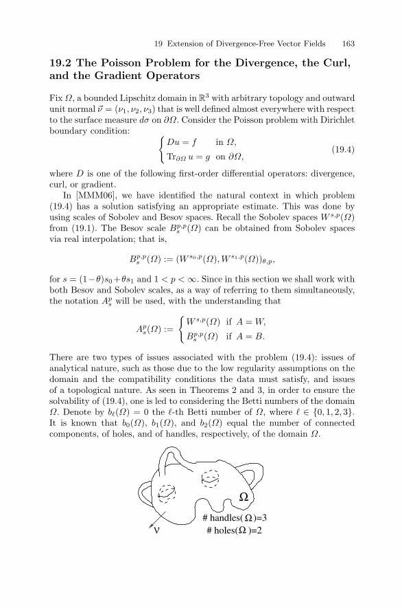
19 Extension of Divergence-Free Vector Fields 163
19.2 The Poisson Problem for the Divergence, the Curl,and the Gradient Operators
Fix Ω, a bounded Lipschitz domain in R3 with arbitrary topology and outward
unit normal #ν = (ν1, ν2, ν3) that is well defined almost everywhere with respectto the surface measure dσ on ∂Ω. Consider the Poisson problem with Dirichletboundary condition:
Du = f in Ω,
Tr∂Ω u = g on ∂Ω,(19.4)
where D is one of the following first-order differential operators: divergence,curl, or gradient.
In [MMM06], we have identified the natural context in which problem(19.4) has a solution satisfying an appropriate estimate. This was done byusing scales of Sobolev and Besov spaces. Recall the Sobolev spaces W s,p(Ω)from (19.1). The Besov scale Bp,p
s (Ω) can be obtained from Sobolev spacesvia real interpolation; that is,
Bp,ps (Ω) := (W s0,p(Ω), W s1,p(Ω))θ,p,
for s = (1−θ)s0 +θs1 and 1 < p < ∞. Since in this section we shall work withboth Besov and Sobolev scales, as a way of referring to them simultaneously,the notation Ap
s will be used, with the understanding that
Aps(Ω) :=
W s,p(Ω) if A = W,
Bp,ps (Ω) if A = B.
There are two types of issues associated with the problem (19.4): issues ofanalytical nature, such as those due to the low regularity assumptions on thedomain and the compatibility conditions the data must satisfy, and issuesof a topological nature. As seen in Theorems 2 and 3, in order to ensure thesolvability of (19.4), one is led to considering the Betti numbers of the domainΩ. Denote by bℓ(Ω) = 0 the ℓ-th Betti number of Ω, where ℓ ∈ 0, 1, 2, 3.It is known that b0(Ω), b1(Ω), and b2(Ω) equal the number of connectedcomponents, of holes, and of handles, respectively, of the domain Ω.

164 D. Mitrea
Let ∇tan denote the tangential gradient on ∂Ω, and let Div, the surface di-vergence, denote its formal adjoint. Then the result concerning the solvabilityof (19.4) when the smoothness index s is close to zero is stated as follows.
Theorem 2. [MMM06] Suppose that Ω is a bounded Lipschitz domain in R3
and that 1 < p < ∞, −1 + 1p < s < 1
p . Then the following are true.
(a) For all f ∈ Aps(Ω) and #g ∈ Bp,p
s+1−1/p(∂Ω, R3) verifying the compatibility
condition
(CC1)
∫
G
f dx =
∫
∂G
#ν · #g dσ
for each connected component G of Ω, there exist #u ∈ Aps+1(Ω, R3) and
C > 0 (independent of #u, f , #g) such that
(P1)
div u = f in Ω,
Tr∂Ω#u = #g on ∂Ω,
and‖#u‖Ap
s+1(Ω,R3) ≤ C‖f‖Aps(Ω) + C‖#g‖Bp,p
s+1−1/p(∂Ω,R3).
(b) b1(Ω) = 0 if and only if for all #f ∈ Aps(Ω, R3) and #g ∈ Bp,p
s+1−1/p(∂Ω, R3)
verifying the compatibility conditions
(CC2)
div f = 0 in Ω,
#ν · #f = −Div(ν × g) on ∂Ω,
there exist #u ∈ Aps+1(Ω, R3) and C > 0 (independent of #u, #f , #g) such that
(P2)
curl u = f in Ω,
Tr∂Ω#u = #g on ∂Ω,
and‖#u‖Ap
s+1(Ω,R3) ≤ C‖#f‖Aps(Ω,R3) + C‖#g‖Bp,p
s+1−1/p(∂Ω,R3).
(c) b2(Ω) = 0 if and only if for all #f ∈ Aps(Ω, R3) and g ∈ Bp,p
s+1−1/p(∂Ω)
verifying the compatibility conditions
(CC3)
curl f = 0 in Ω,
#ν × #f = #ν × (∇tang) on ∂Ω,
there exist u ∈ Aps+1(Ω) and C > 0 (independent of u, #f , g) such that
(P3)
∇u = #f in Ω,
Tr∂Ωu = g on ∂Ω,
and‖u‖Ap
s+1(Ω) ≤ C‖#f‖Aps(Ω,R3) + C‖g‖Bp,p
s+1−1/p(∂Ω).

19 Extension of Divergence-Free Vector Fields 165
Next we state the analog of Theorem 2 when the smoothness index s isaway from zero. The special triplets (0, 0, 0), (1, 0, 0), (0, 1, 0), (0, 0, 1) will bedenoted by (0), e1, e2, and e3, respectively.
Theorem 3. [MMM06] Suppose Ω is a bounded Lipschitz domain in R3 and
1 < p < ∞, −1+ 1p < s−k < 1
p , for some k ∈ N. Then the following are true.
(a) For each f ∈ Aps(Ω) and each family #gα ∈ Bp,p
s+1−1/p(∂Ω, R3), α ∈ N0 with
|α| ≤ k, verifying the compatibility conditions
(CC4)
⎧⎪⎪⎨⎪⎪⎩
(νj∂l − νl∂j)#gα = νj#gα+el− νl#gα+ej
∀α : |α| ≤ k − 1, ∀j, l = 1, 2, 3∫
Gf dx =
∫∂G
#ν · #g(0) dσ,
for each connected component G of Ω, there exist #u ∈ Aps+1(Ω, R3) and
C > 0 (independent of #u, #f , #gα) such that
(P4)
div u = f in Ω,
Tr∂Ω [∂α#u] = #gα on ∂Ω, ∀ |α| ≤ k,
and
‖#u‖Aps+1(Ω,R3) ≤ C‖f‖Ap
s(Ω) + C∑
|α|≤k
‖#gα‖Bp,ps+1−1/p
(∂Ω,R3).
(b) b1(Ω) = 0 if and only if for each #f ∈ Aps(Ω, R3) and each family
#gα ∈ Bp,ps+1−1/p(∂Ω, R3), α ∈ N0 with |α| ≤ k, verifying the compatibility
conditions
(CC5)
⎧⎪⎪⎪⎪⎪⎪⎪⎨⎪⎪⎪⎪⎪⎪⎪⎩
div f = 0 in Ω,
(νj∂l − νl∂j)#gα = νj#gα+el− νl#gα+ej
∀α : |α| ≤ k − 1, ∀ j, l = 1, 2, 3
Tr∂Ω [∂α #f ] = −3∑
j=1
#gα+ej × ej , ∀ |α| ≤ k − 1,
there exist #u ∈ Aps+1(Ω, R3) and C > 0 (independent of #u, #f , #gα) such
that
(P5)
curl u = f in Ω,
Tr∂Ω [∂α#u] = #gα on ∂Ω, ∀ |α| ≤ k,
and
‖#u‖Aps+1(Ω,R3) ≤ C‖#f‖Ap
s(Ω,R3) + C∑
|α|≤k
‖#gα‖Bp,ps+1−1/p
(∂Ω,R3).

166 D. Mitrea
(c) b2(Ω) = 0 if and only if for each #f ∈ Aps(Ω, R3) and each family gα ∈
Bp,ps+1−1/p(∂Ω), α ∈ N0 with |α| ≤ k, verifying the compatibility conditions
(CC6)
⎧⎪⎪⎪⎪⎨⎪⎪⎪⎪⎩
curl f = 0 in Ω,
(νj∂l − νl∂j)gα = νjgα+el− νlgα+ej
∀α : |α| ≤ k − 1, ∀ j, l = 1, 2, 3
Tr∂Ω [∂αfj ] = gα+ej , ∀ j = 1, 2, 3, ∀ |α| ≤ k − 1,
there exist u ∈ Aps+1(Ω) and C > 0 (independent of u, #f , gα) such that
(P6)
∇u = #f in Ω,
Tr∂Ω [∂αu] = gα on ∂Ω, ∀ |α| ≤ k,
and‖u‖Ap
s+1(Ω) ≤ C‖#f‖Aps(Ω,R3) + C
∑
|α|≤k
‖gα‖Bp,ps+1−1/p
(∂Ω).
Theorems 2 and 3 are particular cases of the more general setting of thePoisson problem for the exterior derivative operator with Dirichlet boundarycondition on Lipschitz subdomains of a manifold M , considered in [MMM06].For proofs, see [MMM06].
19.3 Proof of Theorem 1
Fix #u as in (19.2), and define #w by
#w =
#u in Ω1,
0 in R3 \ Ω.
Then clearly #w ∈ Lp(R3\Ω2, R3) and supp #w ⊆ Ω1. In addition, #w ∈ W 1,p(R3\
Ω2, R3) and for each 1 ≤ j ≤ n,
∂j #w =
∂j#u in Ω1,
0 in R3 \ Ω,
where the derivatives are taken in the distributional sense. Indeed, if 〈·, ·〉denotes the pairing between a distribution and a test function, for each #ϕ ∈C∞
0 (R3 \ Ω2,R3), the properties of #u and integration by parts imply that
〈∂j #w, #ϕ〉 = −〈#w, ∂jϕ〉 = −∫
R3\Ω2
#w · ∂j #ϕ = −∫
Ω1
#u · ∂j #ϕ
=
∫
Ω1
(∂j#u) · #ϕ−∫
∂Ω1
Tr∂Ω1#u · #ϕ ν1j dσ =
∫
Ω1
(∂j#u) · #ϕ, (19.5)

19 Extension of Divergence-Free Vector Fields 167
where ν1j is the jth component of the outward unit normal ν1 to Ω1. The last
equality in (19.5) is true since supp(Tr∂Ω1 #u) ⊆ Γ and supp #ϕ ∩ Γ = ∅.Next, define #f := Tr∂(R3\Ω2) #w. From the properties of #w we can conclude
that #f ∈ Bp,p
1− 1p
(∂Ω2,R3), supp #f ⊆ Γ and Tr∂(R3\Ω2)
#f = Tr∂Ω1#u on Γ . Hence,
if ν2 denotes the outward unit normal to Ω2, it follows that∫
∂Ω2
ν2 · #f dσ = −∫
Γ
ν1 · #f dσ = −∫
∂Ω1
ν1 · Tr∂Ω1#u dσ
= −∫
Ω1
div u = 0.
An application of part (a) in Theorem 2 gives the existence of a vector field⎧⎪⎪⎨⎪⎪⎩
#v ∈ W 1,p(Ω2,R3),
div v = 0 in Ω2,
Tr∂Ω2#v = #f ∈ Bp,p
1− 1p
(∂Ω2,R3).
The claim we make is that the vector field
#U :=
#u in Ω1,
#v in Ω2,
verifies (19.3). Clearly, #U ∈ Lp(Ω,R3). Fix #ϕ ∈ C∞0 (Ω,R3) and 1 ≤ j ≤ n.
Then, the properties of #U and integration by parts yield
〈∂j#U, #ϕ〉 = −〈#U, ∂j #ϕ〉 = −
∫
Ω
#U · ∂j #ϕ = −∫
Ω1
#u · ∂j #ϕ−∫
Ω2
#v · ∂j #ϕ
=
∫
Ω1
(∂j#u) · #ϕ−∫
∂Ω1
Tr∂Ω1#u · #ϕ ν1j dσ
+
∫
Ω2
(∂j#v) · #ϕ−∫
∂Ω2
Tr∂Ω2#v · #ϕ ν2j dσ
=
∫
Ω1
(∂j#u) · #ϕ+
∫
Ω2
(∂j#v) · #ϕ. (19.6)
The last equality in (19.6) is a consequence of the fact that the two boundaryintegrals cancel each other since ν1
j = −ν2j on Γ and Tr∂Ω1#u = Tr∂Ω2#v on Γ
while being zero on the rest of their domains. The conclusion is that, ∀ j,
∂j#U :=
∂j#u in Ω1,
∂j#v in Ω2,
and hence, #U ∈ W 1,p(Ω,R3). Furthermore,
168 D. Mitrea
(div #U)|Ω1 = div(#U |Ω1) = div #u = 0,
(div #U)|Ω2 = div(#U |Ω2) = div#v = 0,
so div U = 0 in Ω. We are left with checking that Tr∂Ω#U = 0. This, however,
is true since
(Tr∂Ω#U)|∂Ω2\Γ = (Tr∂Ω2#v)|∂Ω2\Γ = #f |∂Ω2\Γ = 0,
(Tr∂Ω#U)|∂Ω1\Γ = (Tr∂Ω1#u)|∂Ω1\Γ = #f |∂Ω1\Γ = 0.
Finally, that #U satisfies a natural estimate is implicit in the above construc-tion.
19.4 Another Application of Theorem 2
In this section, we discuss the structure of vector fields that play an importantrole in Maxwell’s equations.
Theorem 4. Let Ω be a bounded, convex, Lipschitz domain in R3. Then,
for any 1 < p ≤ 2, and any vector field #u ∈ Lp(Ω, R3) satisfying curl u ∈Lp(Ω, R3), div u ∈ Lp(Ω) and #ν · #u = 0 on ∂Ω can be written in the form
#u = #v + curl ω, (19.7)
#v ∈ W 1,p(Ω,R3), Tr∂Ω#v = 0, #ω ∈ W 1,p(Ω,R3), (19.8)
div ω = 0 in Ω, ∆ ω ∈ Lp(Ω,R3), and ν × ω = 0 on ∂Ω. (19.9)
Moreover, for some C = C(Ω, p) > 0,
‖#v‖W 1,p(Ω,R3) + ‖∆#ω‖Lp(Ω,R3) + ‖#ω‖W 1,p(Ω,R3)
≤ C(‖#u‖Lp(Ω,R3) + ‖curl #u‖Lp(Ω,R3) + ‖div #u‖Lp(Ω)
).
Proof. Since #ν ·#u = 0, by the Divergence Theorem, the compatibility condition(CC1) is satisfied for f := div u and #g = 0. Hence, by Theorem 2 part (a),there exists #v ∈ W 1,p
0 (Ω,R3), with div v = div u in Ω. Thus, if we set #w :=#u− #v, then
#w ∈ Lp(Ω,R3), div w = 0 in Ω, and ν · w = 0 on ∂Ω.
Apply part (b) in Theorem 2 to obtain
#ω′ ∈ W 1,p0 (Ω,R3), curl ω′ = w in Ω.
At this point, we recall a result contained in [Ad93], to the effect thatthere exists ϕ ∈ W 2,p(Ω) ∩ W 1,p
0 (Ω), such that ∆ϕ = div ω′. With this

19 Extension of Divergence-Free Vector Fields 169
function at hand, define #ω := #ω′ − ∇ϕ. Clearly, #ω ∈ W 1,p(Ω,R3). Also,div ω = div ω′ − ∆ϕ = 0 in Ω. In addition, #ν × #ω = 0. The latter followsif we prove that #ν × #ω′ = 0 and #ν ×∇ϕ = 0.
Fix an arbitrary, smooth, compactly supported vector field #ξ in Ω. By thedefinition of #ν×, write
〈#ν × #ω′, #ξ|∂Ω〉 =
∫
Ω
〈curl(ω′), ξ〉 −∫
Ω
〈ω′, curl ξ〉, (19.10)
〈#ν ×∇ϕ, #ξ|∂Ω〉 =
∫
Ω
〈curl(∇ϕ), #ξ〉 −∫
Ω
〈∇ϕ, curl #ξ〉
= −∫
Ω
〈∇ϕ, curl ξ〉 (19.11)
Moreover, since #ω′ ∈ W 1,p0 (Ω,R3) and ϕ ∈ W 1,p
0 (Ω), there exist two sequences
#ψjj and ϕjj of smooth, compactly supported vector fields and functions,
respectively, such that, as j → ∞, #ψj → #ω′ in W 1,p(Ω,R3) and ϕj → ϕ inW 1,p(Ω). As such, also using integration by parts, we have that
∫
Ω
〈curl(#ω′), #ξ〉 = limj→∞
∫
Ω
〈curl(#ψj), #ξ〉 = limj→∞
∫
Ω
〈#ψj , curl #ξ〉 (19.12)
=
∫
Ω
〈#ω′, curl ξ〉, (19.13)
∫
Ω
〈∇ϕ, curl #ξ〉 = limj→∞
∫
Ω
〈∇ϕj , curl #ξ〉 = 0. (19.14)
A combination of (19.10)–(19.14) now yields #ν × #ω = 0.The vectors #v and #ω constructed so far satisfy (19.7)–(19.9). Indeed,
#u = #v + #w = #v + curl ω′ = v + curl ω in Ω; thus, (19.7) holds. The onlycondition from (19.9) left to check is that ∆#ω ∈ Lp(Ω,R3). Observe thatsince div ω = 0, the decomposition of #u from (19.7) implies that −∆#ω =curl curl ω = curl v − curl u, which, based on the properties of #u and #v, is in-deed in Lp(Ω,R3). This concludes the proof of Theorem 4.
Acknowledgement. This work has been partially supported by NSF-FRG grant0456306.
References
[Ad93] Adolfsson, V.: Lp-integrability of the second order derivatives of Greenpotentials in convex domains. Pacific J. Math., 159, 201–225 (1993).
[CCF06] Charina, M., Conti, C., Fornasier, M.: Adaptive frame methods for non-linear variational problems. Numer. Math. (in press).

170 D. Mitrea
[MMM06] Mitrea, D., Mitrea, M., Monniaux, S.: The Poisson problem for the exte-rior derivative operator with Dirichlet boundary condition on nonsmoothdomains. Preprint (2006).
[RS96] Runst, T., Sickel, W.: Sobolev Spaces of Fractional Order, NemytskijOperators, and Nonlinear Partial Differential Operators. de Gruyter,Berlin-New York (1996).
[Tr92] Triebel, H.: Theory of Function Spaces II. Birkhauser, Basel (1992).

20
Solutions of the AtmosphericAdvection–Diffusion Equation by the LaplaceTransformation
D.M. Moreira1, M.T. de Vilhena2, T. Tirabassi3, and B.E.J. Bodmann2
1 Universidade Federal de Pelotas, Bage, RS, Brazil;[email protected]
2 Universidade Federal do Rio Grande do Sul, Porto Alegre, RS, Brazil;[email protected], [email protected]
3 Istituto di Scienze dell’Atmosfera e del Clima, Bologna, Italy;[email protected]
20.1 Introduction
Transport and diffusion models of air pollution are based either on simple tech-niques, such as the Gaussian approach, or on more complex dynamics, such asthe K-theory. The Gaussian equation is an easy method that cannot properlysimulate complex non homogeneous conditions, whereas the K-theory can ac-cept any complex meteorological input, but in general requires tedious numer-ical integration. Gaussian models are still widely used by the environmentalagencies all over the world for regulatory applications. Because of their well-known intrinsic limits, the reliability of a Gaussian model depends strongly onthe determination of dispersion parameters based on the turbulence structureof the PBL. The Gaussian model needs completion by empirically determinedstandard deviations, whereas some commonly measurable turbulent exchangecoefficient has to be introduced into the advection–diffusion equation. Ana-lytical solutions to the complete advection–diffusion equation cannot be givenbut in a few specialized cases [Tir03], and numerical solutions cannot be easily“interpreted” as the simple Gaussian model. As a consequence, the major partof applications to practical problems are currently done by using the Gaussianmodel, and a great deal of empirical work has been done do determine thesigmas appropriate for the PBL under various meteorological conditions andto extend the basic formulation of this model and its range of applicability[Zan90].
The advection–diffusion equation is believed to give a better representationof the effects due to the vertical stratification of the atmosphere. To relate toprevious types of models, we employ an analytical solution of the advection–diffusion equation that accepts height-independent wind and eddy diffusivity
172 D.M. Moreira et al.
coefficients, and subdivide the PBL into several layers, in which the eddydiffusivity and wind speed are considered with their average values. The hybridmodel then represents conditions of a height-structured PBL [Vil98].
20.2 The Advection–Diffusion Equation
The advection–diffusion equation for air pollution in the atmosphere is essen-tially a statement of conservation of the suspended material:
∂C
∂t+ u
∂C
∂x+ v
∂C
∂y+ w
∂C
∂z= −∂u′c′
∂x− ∂v′c′
∂y− ∂w′c′
∂z+ S,
where C denotes the average concentration, u, v, w are the Cartesian compo-nents of the wind, and S is the source term. The terms u′c′, v′c′, and w′c′
represent the turbulent fluxes of contaminants in the longitudinal, crosswind,and vertical directions. The concentration turbulent fluxes are assumed to beproportional to the mean concentration gradient, which is known as Fick the-ory u′c′ = −Kx
∂C∂x , v′c′ = −Ky
∂C∂y , w′c′ = −Kz
∂C∂z , where Kx, Ky, Kz are the
Cartesian components of eddy diffusivity and z is the height. This assump-tion, combined with the continuity equation, leads to the advection–diffusionequation. The crosswind integration yields with C =
∫ ∞−∞ C(x, y, z) dy the
crosswind integrated concentration
∂C
∂t+ u
∂C
∂x+ w
∂C
∂z=
∂
∂x
(Kx
∂C
∂x
)+
∂
∂z
(Kz
∂C
∂z
)+ S.
Before applying the Laplace transformation, we perform a stepwise ap-proximation of these coefficients. To this end, we discretize the height zi
of the PBL into N subintervals such that inside each subregion, K andu assume average values given by Kn = (zn+1 − zn)−1
∫ zn+1
znKz(z) dz and
un = (zn+1 − zn)−1∫ zn+1
znuz(z) dz for n = 1, . . . , N. In scenarios where the
vertical eddy diffusivity depends on x and z, one proceeds in a similar fashion,first determining the average in z followed by averaging in x, so that Km,n
is double-indexed with n for the vertical segments and m = 1, . . . , M for thelongitudinal ones. The solution may now be determined for each segment.
20.3 The Laplace Transformation Solution
The one-dimensional time-dependent advection–diffusion equation is ∂C∂t =
∂∂z
(Kz
∂C∂z
)for 0 < z < zi and t > 0, subject to the boundary conditions
Kz∂C∂z = 0 at z = 0, zi and with initial condition C(z, 0) = Qδ(z − Hs) at
t = 0, where Hs is the source height and Q is the emission rate. Assuming thatthe nonhomogeneous turbulence is modeled by an eddy diffusivity depending

20 Solutions of the Atmospheric Advection–Diffusion Equation 173
on the z-variable, the Laplace transformation is applied, which changes the
advection-diffusion equation ∂Cn
∂t = Kzn∂2Cn
∂z2 for each interval zi < z < zi+1
and n = 1, . . . , N to the form
∂2
∂z2Cn(z, s) − s
KznC(z, s) = − 1
KznCn(z, 0).
Here Cn(z, s) = LCn(z, t); t → s denotes the Laplace transform of Cn(z, t)with respect to the t-variable, which has the well-known solution
Cn(z, s) = Ane−Rnz + BneRnz − Q
Racosh (Rn(z − Hs))H(z − Hs), (20.1)
where H(z−Hs) is the Heaviside function, Rn =√
s/Kzn, and Ra =√
Kzns.Note that at this stage there are 2N integration constants, which are reducedby the (2N − 2) interface conditions, namely, the continuity of concentration
Cn = Cn+1 and flux concentration at the interface: Kzn∂cn
∂z = Kzn+1∂cn+1
∂z ,for n = 1, . . . , N − 1. Then, by (20.1), we obtain the system
⎛
⎜
⎜
⎜
⎜
⎜
⎜
⎜
⎜
⎜
⎜
⎜
⎝
M11 M12 0 0 0 0 . . . 0M21 M22 M23 M24 0 0 . . . 0M31 M32 M33 M34 0 0 . . . 00 0 M43 M44 M45 M46 . . . 00 0 M53 M54 M55 M56 . . . 0...
......
......
......
...0 0 0 . . . Mn−1,n−3 Mn−1,n−2 Mn−1,n−1 Mn−1,n
0 0 0 0 0 . . . Mn,n−1 Mn,n
⎞
⎟
⎟
⎟
⎟
⎟
⎟
⎟
⎟
⎟
⎟
⎟
⎠
⎛
⎜
⎜
⎜
⎜
⎜
⎜
⎜
⎜
⎜
⎜
⎜
⎜
⎜
⎝
A1
B1
A2
B2
...
...An
Bn
⎞
⎟
⎟
⎟
⎟
⎟
⎟
⎟
⎟
⎟
⎟
⎟
⎟
⎟
⎠
=
⎛
⎜
⎜
⎜
⎜
⎜
⎜
⎜
⎜
⎜
⎜
⎜
⎜
⎜
⎝
0...0
Dn∗
D′
n∗
0...0
⎞
⎟
⎟
⎟
⎟
⎟
⎟
⎟
⎟
⎟
⎟
⎟
⎟
⎟
⎠
,
where the Mij are given byM11=R1, M2n,2n+1=−eRnzn , M2n+1,2n+1=−Kn+1Rn+1e
Rn+1zn ,M12=−R1, M2n,2n+2=−e−Rnzn , M2n+1,2n+2=Kn+1Rn+1e
−Rn+1zn ,M2n,2n−1=eRnzn , M2n+1,2n−1=KnRneRnzn , Mn,n−1=RNeRN zN ,M2n,2n=e−Rnzn , M2n+1,2n=−KnRne−Rnzn , Mn,n=−RNe−RN zN ,
and in the sublayer of contaminant emission, Dn∗ = − QRa
cosh (Rn(z − Hs))and D′
n∗ = −Q cosh (Rn(z − Hs)). Solving this linear system and invertingthe transformed concentration by the Gaussian quadrature scheme, we finallyget the solution
Cn(z, t) =
k∑
i=1
aipi
t
[Ane−Rnz + BneRnz − Q
Racosh (Rn(z − Hs))H(z − Hs)
],
(20.2)where k is the number of quadrature points, Rn =
√pi/(tKzn), and Ra =√
Kznpi/t. Here ai and pi are the Gaussian quadrature parameters (see[Str66]).
The two-dimensional steady-state advection–diffusion equation is of the
form u∂C∂x = ∂
∂z
(Kz
∂C∂z
)for 0 < z < zi and x > 0, subject to the

174 D.M. Moreira et al.
boundary conditions Kz∂C∂z = 0 at z = 0, zi and the source condition
C(0, z) = Qu δ(z − Hs) at x = 0. Here Hs is the height source and Q is the
continuous contaminant emission rate. Proceeding as in the previous section,we perform the stepwise approximation of the parameters, apply the Laplacetransformation with respect to the x-variable, solve the resulting set of ordi-nary differential equations, and apply the boundary and interface conditionsto determine the integration constants. This procedure leads to the solution
Cn(x, z) =
m∑
i=1
aipi
x
[Ane
−Rnz +BneRnz − Q
Racosh (Rn(z −Hs))H(z −Hs)
],
(20.3)
where m is the number of quadrature points, Rn =√
unpi
Kznx , and Ra =√unKzn
pi
x .The two-dimensional steady-state equation with longitudinal diffusion is
u∂C∂x = ∂
∂x
(Kx
∂C∂x
)+ ∂
∂z
(Kz
∂C∂z
)for 0 < z < zi and x > 0, subject
to the boundary conditions Kz∂C∂z = 0 at z = 0, zi and the source con-
dition C(0, z) = Qu δ(z − Hs) at x = 0. A procedure similar to the one
above yields solution (20.3) if this time we substitute QRa
→ QRb
Ra, where
Rn =√Rbpiun/(xKzn), Ra =
√unKznpi/x, and Rb = 1 − pi/Pe. Here
Pe = unx/Kxn is the Peclet number, which essentially represents the ra-tio between the advective and diffusive transport terms. Small values of thisnumber are related to a weak wind, which turns the downwind diffusion impor-tant and the region of interest (i.e., region of height concentrations) remainsclose to the source. On the other hand, for large values of the Peclet number,the downwind diffusion may be neglected when compared with the transportadvective term. This corresponds to a large distance to the source. The so-lution reduces to (20.3) when the longitudinal eddy diffusivity tends to zero(Kx → 0).
The two-dimensional time-dependent advection–diffusion equation is ∂C∂t +
u∂C∂x = ∂
∂z
(Kz
∂C∂z
)for 0 < z < zi, x > 0, and t > 0, subject to the boundary
conditions Kz∂C∂z = 0 at z = 0, zi, the source condition C(0, z, t) = Q
u δ(z−Hs)at x = 0, and the initial condition C(x, z, 0) = 0 at t = 0. The solution of thissystem is
Cn=
k∑
i=1
aipi
t
m∑
j=1
ajpj
x
[Ane
−Rnz+BneRnz−QRb
Racosh (Rn(z−Hs))H(z−Hs)
],
(20.4)
where Rn =√
pi
tKzn+
unpj
Kznx and Ra =√
pi
t Kzn + unKznpj
x . Solution (20.4)
reduces to (20.3) as time tends to infinity.Consider the advection–diffusion equation including a decaying contami-
nant (i.e., a radioactive contaminant) emission as source term (S = −λC).

20 Solutions of the Atmospheric Advection–Diffusion Equation 175
The dynamical equation is
∂C
∂t+ u
∂C
∂x+ w
∂C
∂z=
∂
∂x
(Kx
∂C
∂x
)+
∂
∂z
(Kz
∂C
∂z
)− λC
for 0 < z < zi, x > 0, and t > 0, with λ the decay constant, and subjectto the boundary conditions Kz
∂C∂z = 0 at z = 0, zi, the source condition
C(0, z, t) = Qu δ(z −Hs) at x = 0, and the initial condition C(x, z, 0) = 0 at
t = 0. Application of the previous procedure leads to solution (20.4), but with
Rn = wn
2Kzn± 1
2
√(wn
2Kzn
)2
+ 4Kzn
[p− α+ sun
(1 − Kxns
un
)], Rb = 1− pj
Pe, and
Ra =
√w2
n + 4Kzn
[p− α+ sun
(1 − Kxns
un
)]. This solution reduces to (20.3)
as Kx → 0, t → ∞, and α = w = 0.
20.4 Advection–Diffusion Considering Non-FickianTurbulence Closure
The downgradient transport hypothesis is often inconsistent with observedfeatures of turbulent diffusion in the upper portion of the mixed layer, wherecountergradient material fluxes are known to occur [Dea75]. In the sequel, wereport the solution of the advection–diffusion equation considering nonlocaleffects in the turbulence closure.
The one-dimensional time-dependent equation reads as ∂C∂t = −∂w′c′
∂z for0 < z < zi and t > 0, assuming the non-Fickian closure of turbulence[1 +(
SkTLw σw
2
)∂∂z + τ ∂
∂t
]w′c′ = −Kz
∂C∂z proposed by van Dop and Verver
[Van03]. Here Sk is the skewness, TLw is the vertical Lagrangian time scale,σw is the vertical turbulent velocity variance, and τ is the relaxation time.Then the resulting dynamics is
τ∂2C
∂t2+∂C
∂t+
(SkTLwσw
2
)∂2C
∂t∂z=
∂
∂z
(Kz
∂C
∂z
),
subject to the boundary conditions Kz∂C∂z = 0 at z = 0, zi and the initial
condition C(z, 0) = Qδ(z − Hs) at t = 0. The solution of this system usesH = H(z −Hs) and is given by
Cn=
k∑
i=1
ajpi
teF ∗
N (z−Hs)
[Ane
R∗nz+Bne
−R∗nz−τPjQ
R∗a
cosh (R∗n(z−Hs))H
],
(20.5)
where R∗n =
√β2
np2i +4Kznpi(τpi+t)
2Kznt , R∗a =
√β2
np2i + 4Kznpi(τpi + t), F ∗
n =βpi
2Kznt , and βn =SkσwTLw
2 . Solution (20.5) reduces to (20.2) as βn and τtend to zero.

176 D.M. Moreira et al.
Finally, we analyze the solution of u∂C∂x = −∂w′c′
∂z , assuming the non-Fickian closure of turbulence as in the preceding case but with τ = 0:
u∂C
∂x+
∂
∂z
(uSkTLw
2
∂C
∂x
)=
∂
∂z
(Kz
∂C
∂z
)
for 0 < z < zi and x > 0, subject to the boundary conditions Kz∂C∂z = 0
at z = 0, zi and the source condition C(0, z) = Qu δ(z − Hs) at x = 0. The
solution is
Cn=
m∑
i=1
aipi
xeF ∗
nz
[Ane
R∗nz+Bne
−R∗nz−Q
R∗a
cosh (R∗n(z−Hs))H(z−Hs)
],
(20.6)
where R∗n = 1
2
√(βnpi
Kznx
)2+ 4unpi
Kznx , R∗a =
√β2
np2i + 4Kznpi(τpi + t), F ∗
n =
βpi
2Kznt , and βn =unSkσwTLw
2 . Here solution (20.6) reduces to (20.3) as βn → 0.
20.5 Model Performance Evaluation AgainstExperimental Data
In order to illustrate the aptness of the discussed formulation to simulatecontaminant dispersion in the PBL, we evaluate the performance of solution(20.4) against experimental crosswind ground-level concentration using tracerSF6 data from two different dispersion experiments. The first one, carried outin the northern part of Copenhagen, is described in [Gry87]. The tracer wasreleased without buoyancy from a tower at a height of 115 m and was collectedat the ground-level positions at a maximum of three crosswind arcs of tracersampling units. The sampling units were positioned at 2 to 6 km from thepoint of release. The site was mainly residential with a roughness length of0.6 m. The PBL was parameterized assuming the eddy diffusivity proposed by[Deg01], that is, Kz = 0.55σwz/(4(f∗
m)w), where (f∗m)w is the vertical normal-
ized frequency of spectral peak and σw is the vertical wind velocity variance.The wind speed profile has been parameterized following the similarity the-ory of Monin–Obukhov [Ber86]: u(z) = u∗
k [ln(z/z0) − Ψm(z/L) + Ψm(z0/L)]if z ≤ zb, u(z) = u(zb) if z > zb, where zb = min[|L|, 0.1h], Ψm is a stabilityfunction given by Ψm = 2 ln((1+A)/2)+ln((1+A2)/2)−2 tan−1 A+π/2 withA = (1− 16z/L)1/4, k = 0.4 is the Von Karman constant, z0 is the roughnesslength, u∗ is the friction velocity, and L is the Monin–Obukhov length.
Figure 20.1 (left) shows the scatter diagrams between the measured andpredicted crosswind integrated concentrations using the above parameteriza-tions for wind and eddy diffusivities profiles. A good agreement is observedbetween the results.
The modulus of the real part of the root of the Gaussian quadraturescheme for the Laplace transform inversion increases with N (the order of

20 Solutions of the Atmospheric Advection–Diffusion Equation 177
Fig. 20.1. The scatter diagram for the semi-analytical solution (20.4) for the Copen-hagen experiment (left) and the Kinkaid experiment (right): observed (Co) and pre-dicted (Cp) crosswind ground-level integrated concentration (k = 2, m = 8, ∆z = 40m). Points between lines diverge by less than a factor of 2.
the approximation). The solution for the Laplace-transformed concentrationhas exponential terms; we observed from numerical simulation the appearanceof overflows for a positive argument of the exponential and underflow for anegative argument when k and m assume values larger than 8 (on a PC with32-bit precision). With this restriction, we get results with good statisticalaccuracy.
One observes that the curves for concentrations in Figure 20.2, especiallyfor the lower time values with the increase of the quadrature points, presenta nonphysical oscillatory behavior except for k = 2. In Figure 20.3, we showthe dimensionless ground-level concentration C = Cuzi/Q as a function ofthe dimensionless time t∗ = tw∗/zi for the source distances x = 1000 m andx = 3000 m, considering k = 2 and m = 8; we observed that the steady-stateconcentration field is obtained as t∗ tends to infinity.
In Figure 20.4, we present an analysis of the influence of the number ofquadrature points on the solution. Figure 20.4(a) shows the result for the sta-tionary problem (20.3) as a function of the number of quadrature points withits numerical convergence of the results encountered for dimensionless ground-level concentration as a function of the quadrature points m. In Figure 20.4(b),we display the results for problem (20.4) for a steady-state condition. Finally,note the small oscillations of the concentration in Figure 20.4(b), caused byoverflow and underflow. The behavior of the solution can be improved byusing multiple precision methods.
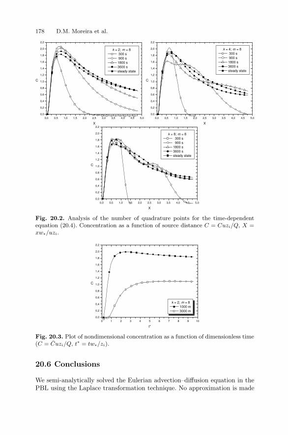
178 D.M. Moreira et al.
Fig. 20.2. Analysis of the number of quadrature points for the time-dependentequation (20.4). Concentration as a function of source distance C = Cuzi/Q, X =xw∗/uzi.
Fig. 20.3. Plot of nondimensional concentration as a function of dimensionless time(C = Cuzi/Q, t∗ = tw∗/zi).
20.6 Conclusions
We semi-analytically solved the Eulerian advection–diffusion equation in thePBL using the Laplace transformation technique. No approximation is made

20 Solutions of the Atmospheric Advection–Diffusion Equation 179
(a) (b)
Fig. 20.4. Analysis of the number of quadrature points: (a) for (20.3); (b) steady-state condition in (20.4).
in its derivation except for the stepwise approximation of the parameters andthe Laplace numerical inversion by the Gaussian quadrature scheme. It is wellknown that the results obtained by the Gaussian quadrature scheme of orderN are exact when the transformed function is a polynomial of degree 2N − 1.On the other hand, from the Weierstrass approximation theorem, it is knownthat a continuous function can be approximated by a polynomial, and thatthe approximation improves with the increase of the degree of the polynomial.This means that increasing k and m in the Gaussian quadrature schemes forthe concentration solution, one expects the numerical results to converge tothe exact result. The error estimation from numerical results with k + 1 andk points of quadrature and for m + 1 and m points permits us to control theerror in the Gaussian quadrature scheme by properly choosing k and m, inorder to reach a prescribed accuracy.
According to the Lax equivalence theorem for linear problems [Kyt97],the convergence of the numerical schemes demands stability and consistency.To accomplish the stability conditions, the numerical methods impose a largenumber of step calculations, performing the time integration for most times.Our solution allows us to perform the calculation at any time. This fact justi-fies the smaller computational time as well as the smaller round-off error influ-ence in the accuracy of the results when compared with the numerical ones.The above arguments and the good agreement between the semi-analyticalresults and experimental data make us confident that our hybrid method is arobust approach for simulating the pollutant dispersion in the PBL.
Acknowledgement. The authors thank CNPq and FAPERGS for the partial financialsupport of this work.

180 D.M. Moreira et al.
References
[Ber86] Berkovicz, R.R., Olesen, H.R., Torp, U.: The Danish Gaussian air pollu-tion model (OML). In: Proceedings 15th Internat. Tech. Meeting on AirPollution Modeling and Its Applications V, Plenum, St. Louis, MO (1986).
[Dea75] Deardoff, J.W., Willis, G.E.: A parameterization of diffusion into the mixedlayer. J. Appl. Meteorol., 14, 1451–1458 (1975).
[Deg01] Degrazia, G.A., Moreira, D.M., Vilhena, M.T.: Derivation of an eddy dif-fusivity depending on source distance for vertically inhomogeneous turbu-lence in a Convective Boundary Layer. J. Appl. Meteorol., 40, 1233–1240(2001).
[Gry87] Gryning, S.E., Holtslag, A.A.M., Irwin, J.S., Siversteen, B.: Applied dis-persion modelling based on meteorologing scaling parameters. Atmos. En-viron., 21, 79–89 (1987).
[Han89] Hanna, S.R., Paine, R.J.: Hibrid plume dispersion model (HPDM) devel-opment and evaluation, J. Appl. Meteorol., 28, 206–224 (1989).
[Kyt97] Kythe, P.K., Puri, P., Schferkotter, M.R.: Partial Differential Equationsand Mathematics. CRC Press, Boca Raton, FL (1997).
[Mor99] Moreira, D.M., Degrazia, G.A., Vilhena, M.T.: Dispersion from low sourcesin a convective boundary layer: an analytical model. Il Nuovo Cimento,22C, 685–691 (1999).
[Str66] Stroud, A.H., Secrest, D.: Gaussian Quadrature Formulas. Prentice Hall,Englewood Cliffs, NJ (1966).
[Tir03] Tirabassi, T.: Operational advanced air pollution modeling. Pure Appl.Geophys., 160, 5–16 (2003).
[Van03] van Dop, H., Verver, G.: Countergradient transport revisited. J. Atmos.Sci., 58, 2240–2247 (2001).
[Vil98] Vilhena, M.T., Rizza, U., Degrazia, G.A., Mangia, C., Moreira, D.M.,Tirabassi, T.: An analytical air pollution model: development and eval-uation. Control Atmos. Phys., 71, 315–320 (1998).
[Zan90] Zanetti, P.: Air Pollution Modeling. Computational Mechanics Publica-tions, Southampton (1990).
21
On Quasimodes for Spectral Problems Arisingin Vibrating Systems with ConcentratedMasses
E. Perez
Universidad de Cantabria, Santander, Spain; [email protected]
21.1 Introduction
Quasimodes for positive, symmetric, and compact operators on Hilbert spacesarise often in the literature in the description of behavior at high-frequencyvibrations (see, for example, [Arn72], [BB91], [Laz99], and [Per03]). Roughlyspeaking, the quasimodes u can be defined as functions approaching a certainlinear combination of eigenfunctions associated with eigenvalues in “smallintervals” [λ − r, λ + r]. Their usefulness in describing asymptotics for lowfrequency vibrations in certain singularly-perturbed spectral problems hasbeen made clear recently in many papers (see [LP03], [Per04], [Per05], [Per06],and [Per07]).
In this chapter, we consider a vibrating system with concentrated masses.Namely, we consider the vibrations of a body occupying a domain Ω of R
n,n = 2, 3, that contains many small regions (Bε) of high density—so-calledconcentrated masses—near the boundary. The small parameter ε deals withthe size of the masses, their number, and their densities. The asymptoticbehavior, as ε → 0, of the eigenelements (λε, uε) of the corresponding spectralproblem, namely problem (21.3), when λε = O(εm−2), has been treated in[Per04] (see [LP03] for a substantial list of references on the subject). Here,considering the hyperbolic problem (21.15), we provide estimates for the timet in which certain standing waves approach time-dependent solutions when theinitial data are quasimodes. Also, precise bounds for the discrepancies betweenthe solutions and standing waves in suitable Hilbert spaces are provided. Theresults can be extended to high-frequency vibrations.
It should be mentioned that in certain problems arising in spectral per-turbation theory, the eigenfunctions associated with low frequencies give riseto vibrations of the system that are concentrated asymptotically in a certainregion, and that it is possible to construct quasimodes associated with highfrequencies that give rise to other kinds of vibrations. This is the case, for in-stance, with spectral stiff problems [LP97] or vibrating systems with a singleconcentrated mass (see [GLP99] and [Per03]).

182 E. Perez
Nevertheless, when the low frequencies converge toward the same positivevalue µ (see [LP03], [Per05], and [Per07]), it can be difficult to describe theasymptotic behavior, as ε → 0, of the individual eigenfunctions and to obtainasymptotics for the first eigenfunction. In some of these problems, quasimodesuε that provide an approach to linear combinations of eigenfunctions associ-ated with all the eigenvalues in intervals [µ−δε, µ+δε], with δε → 0 as ε → 0,can be constructed. These quasimodes could concentrate asymptotically theirsupport or their energy at points or thin layers. This happens, for example,when describing vibrations of systems with many concentrated masses nearthe boundary (see [LP03], [Per05], and [Per06]), or in models from geophysics([BI06] and [Per07]).
For these vibrating systems, given the quasimode as an initial data, thesolution of the evolution problem behaves as a standing wave affecting onlysmall regions for a long period of time, which we determine in this chapter.Here we prove that, when considering the evolution problem (21.15), for along time, namely, for t ∈ [0, O((δε)−δ)] with some positive δ, the solutions of(21.15) are approached through standing waves of the type ei
√µtuε. It turns
out that the results hold for any eigenvalue µ of the local problem (21.4).We emphasize that the results in this chapter can be stated in a more
general abstract framework and extend to low-frequency and high-frequencyvibrations of other vibrating systems (see [LP01], [LP03], [Per03], [Per04], and[Per06]). We also note that these results are very different from those in [LP93]and [LP95b], where the evolution problem (21.15) is used to derive results onspectral convergence for low frequencies, which are much weaker than thosein Theorem 2.
Section 21.2 contains preliminary results on quasimodes for problem (21.3).Proofs of these results can be found in [Per04], [Per05], and [Per06]. Section21.3 contains new results on the ε-dependent evolution problem (21.15) (seeTheorem 3 and Remark 1). For brevity, we sketch only an idea of the proof.
21.2 The Spectral Problem
Let A : H −→ H be a linear, self-adjoint, positive, and compact operator ona separable Hilbert space H. Let λ−1
i ∞i=1 be the set of positive eigenvalues
with the usual convention for repeated eigenvalues, λi → ∞ as i → ∞. Letui∞
i=1 be the set of eigenfunctions, which form an orthonormal basis for H.A quasimode with remainder r > 0 for the operator A is a pair (u, µ) ∈
H × R, with ||u||H = 1 and µ > 0, such that ||Au− µu||H ≤ r. If there is noambiguity, u is also referred to as a quasimode.
The following result establishes the closeness in the space H × R of theeigenelements of the operator A to a given quasimode of A (see, for example,[OSY92] for a proof, and [Laz99] for a more general statement).

21 Quasimodes for Spectral Problems 183
Theorem 1. Given a quasimode (u, µ) with remainder r for A, in each in-terval [µ − r∗, µ + r∗] containing [µ − r, µ + r], there are eigenvalues of theoperator A, λ−1
i(r∗)+kk=1,2,...,I(r∗) for some index i(r∗) and number I(r∗) ≥ 1.
In addition, there is u∗ ∈ H, ‖u∗‖H = 1, u∗ =∑I(r∗)
k=1 αkui(r∗)+k for certainconstants αk, and satisfying
‖u − u∗‖H = ‖u −I(r∗)∑
k=1
αkui(r∗)+k‖H ≤ 2r
r∗ . (21.1)
From the literature on spectral perturbation problems it appears that,when Theorem 1 is applied, the spaces and operators under considerationoften depend on a small parameter ε that converges to 0. Also, the functionu and the numbers λ and r arising in the definition of a quasimode dependon this parameter. This is the case of the operators associated with vibratingsystems with concentrated masses, namely, problem (21.3), which we studyin this chapter. For the sake of completeness, in Subsection 21.2.1 we gathercertain results on quasimodes for this problem (21.3), used subsequently inthe proof of the results in Section 21.3.
21.2.1 The Spectral Perturbation Problem
Let Ω be a bounded domain of Rn, n = 2, 3, with a Lipschitz boundary ∂Ω.
Let Σ and ΓΩ be nonempty parts of the boundary such that ∂Ω = Σ ∪ ΓΩ ;Σ is assumed to be in contact with xn = 0. Let ε and η be two smallparameters such that ε ≪ η and η = η(ε) → 0 as ε → 0.
For n = 2, let B be the semicircle B = (y1, y2) / y21 + y2
2 < 1, y2 < 0in the auxiliary space R
2 with coordinates y1, y2. For n = 3, let B be thehalf-ball B = (y1, y2, y3) / y2
1 +y22 +y2
3 < 1, y3 < 0 in the auxiliary space R3
with coordinates y1, y2, y3. Let ∂B be the boundary of B, ∂B = T ∪ Γ , whereT is the part lying on yn = 0. Let Bε (and, similarly, T ε, Γ ε) denote itshomothetic εB (εT , εΓ ). Let Bε
k (and, similarly, T εk , Γ ε
k ) denote the domainobtained by the translation of the previous Bε (T ε, Γ ε) centered at the pointxk of Σ at distance η between them. Here k is a parameter ranging from 1 toN(ε), k ∈ N. N(ε) denotes the number of Bε
k contained in Ω; N(ε) is O(η−1)for n = 2 and O(η−2) for n = 3. The parameter α denotes the value
α = limε→0
−1
η ln εfor n = 2 and α = lim
ε→0
ε
η2for n = 3. (21.2)
We consider the eigenvalue problem⎧⎪⎨⎪⎩
−∆uε = ρελεuε in Ω,
uε = 0 on ΓΩ ∪⋃T ε,∂uε
∂n = 0 on Σ −⋃T ε,
(21.3)
where ρε = ρε(x) is the density function defined by

184 E. Perez
ρε(x) =1
εmif x ∈
⋃Bε, ρε(x) = 1 if x ∈ Ω −
⋃Bε,
the symbol⋃
is extended, for fixed ε, to all the regions Bεk contained in Ω, and
the parameter m is a real number, m > 2 (see [LP93]–[LP95b] for differentvalues of the parameter m, boundary conditions, and domain shapes).
As is well known, problem (21.3) has a discrete spectrum. For fixed ε,let λε
i∞i=1 be the sequence of eigenvalues of (21.3), converging to ∞, with
the classical convention for repeated eigenvalues. It has been proved (see[LP93]–[LP95b]) that they satisfy the estimates Cεm−2 ≤ λε
i ≤ Ciεm−2,
where C is a constant independent of ε and i and Ci is a constant inde-pendent of ε. Let uε
i∞i=1 be the corresponding sequence of eigenfunctions,
which is an orthogonal basis for the space Vε, where Vε is the completion ofu ∈ D(Ω) / u = 0 on ΓΩ ∪ ⋃
T ε in the topology of H1(Ω).Convergence results for the low frequencies, the eigenvalues of order
O(εm−2) of (21.3), and the associated eigenfunctions can be found in [Per04],[Per05], and [Per06]. Also, the limit behavior of the eigenelements for se-quences of eigenvalues of order O(1), the so-called high frequencies, is in[LP93], [LP95a], [LP95b], and [LP01]. As in the case of a single concentratedmass, in general, low frequencies are associated with the local vibrations of theconcentrated masses, each one independent of the others. We have found onlyone exception: For n = 3 and α > 0, these frequencies also give rise to globalvibrations affecting the whole structure ([LP03]). Apart from this exception,the low frequencies and the corresponding eigenfunctions are asymptoticallydescribed, in a certain way, by a so-called local eigenvalue problem (21.4).
The local problem is posed in Rn− = y ∈ R
n / yn < 0 as follows:
⎧⎪⎪⎪⎪⎪⎪⎪⎪⎪⎨⎪⎪⎪⎪⎪⎪⎪⎪⎪⎩
−∆yU = λU in B,
−∆yU = 0 in Rn− − B,
[U ] = [ ∂U∂ny
] = 0 on Γ,
U = 0 on T , ∂U∂yn
= 0 on yn = 0 − T ,
U(y) → c, as |y| → ∞ , yn < 0 when n = 2,
U(y) → 0, as |y| → ∞ , yn < 0 when n = 3 ,
(21.4)
where the brackets denote the jump across Γ , ny is the unit outward normalto Γ , and c is some unknown but well-defined constant. The variable y is thelocal variable:
y =x − xk
ε.
Problem (21.4) can be written as a standard eigenvalue problem with a
discrete spectrum in the space V, where V is the completion of U ∈D(Rn−) / U = 0 on T in the Dirichlet norm ‖∇yU‖L2(Rn−) (see [LP93] and[LP95b]).

21 Quasimodes for Spectral Problems 185
Theorem 2 allows us to assert that there are at least l0N(ε) valuesλε
i(ε)/εm−2 converging to each eigenvalue λ0 of (21.4), with l0 being the multi-
plicity of λ0. The corresponding eigenfunctions Uε [cf. (21.5)] are approached
in the space Vε by the eigenfunctions of (21.4) associated with λ0, concentrat-ing their support asymptotically in neighborhoods of the concentrated massesas stated in Theorem 2.
Also, the results in Theorem 2 along with the results on comparison ofspectra for perturbed domains in [Per05] allow us to obtain an importantdifference for the asymptotic behavior of the low frequencies between thedimensions n = 2 and n = 3 of the space. Namely, for n = 2, and for eachi = 1, 2, . . . , λε
i /εm−2 → λ01, as ε → 0, where λ0
1 is the first eigenvalue of(21.4). This does not hold for n = 3 and the value of α in (21.2) strictlypositive (see [Per05] and [Per06] for further explanations). Let us refer to[GLP99], [OSY92], and [SS89] to compare with the stronger results on theapproach for the eigenfunctions in the case of a single concentrated mass, thecase where the convergence of the rescaled spectrum of (21.3) to that of (21.4)with conservation of multiplicity holds.
Let us change the variable in (21.3) by setting y = x/ε. We obtain:
∫
Ωε
∇yUε.∇yV ε dy =λε
εm−2
∫
Ωε
βε(y)UεV ε dy, ∀V ε ∈ Vε, (21.5)
with Ωε being the domain y / εy ∈ Ω and βε(y) in (21.5) defined as
βε(y) = 1 if y ∈⋃
τyBε, and βε(y) = εm if y ∈ Ωε −
⋃τyBε, (21.6)
where τyBε denote the transformed domains of the regions Bε to the y vari-
able. Vε is the functional space U = U(y) /U(εy) ∈ Vε. We assume thatthe eigenfunctions Uε
i ∞i=1, in the local variable, satisfy ‖Uε‖
Vε = 1.
Let us introduce the self-adjoint positive and compact operator Aε on Vε,Aε defined by the right-hand side of (21.5), namely,
〈AεU, V 〉Vε =
∫⋃
τyBε
UV dy + εm
∫
Ωε−⋃
τyBε
UV dy, ∀U, V ∈ Vε, (21.7)
with eigenelements (εm−2/λεi , U
εi )∞
i=1.Let us consider λ0 an eigenvalue of (21.4) of multiplicity l0, and let U0
1 ,
U02 , . . . , U
0l0
be the corresponding eigenfunctions, orthogonal in V and satisfy-ing ‖∇yU
0i ‖L2(Rn−) = 1.
Let us introduce a function ϕε(y) that depends on n. For n = 2, we consider
Rε =√
ε+η/4ε and define ϕε(y) = 0 if |y| ≥ R2
ε,
ϕε(y) = 1 if |y| ≤ Rε, ϕε(y) = 1 − ln |y| − lnRε
lnRεif Rε ≤ |y| ≤ R2
ε. (21.8)

186 E. Perez
For n = 3, we consider ϕε as a smooth function that takes the value 1 inthe semi-ball of radius ((ε+ η/8)/ε), B((ε+ η/8)/ε), and is 0 outside thesemi-ball of radius ((ε+ η/4)/ε), B((ε+ η/4)/ε):
ϕε(y) = ϕ
(2|εy| − ε
η
), (21.9)
where ϕ ∈ C∞[0, 1], 0 ≤ ϕ ≤ 1, ϕ = 1 in [0, 1/4], and Supp(ϕ) ⊂ [0, 1/2].
Obviously, the elements of Vε extended by zero in Rn− −Ωε are elements
of V. Moreover, we have (see [LP93] and [LP95b]) that U0p ϕ
ε ∈ Vε, and, as
ε → 0, U0p ϕ
ε −→ U0p in V.
For each k = 1, 2, . . . , N(ε), p = 1, 2, . . . , l0, we introduce the function
Zεk,p(y) =
U0p (y − xk
ε )ϕε(y − xk
ε )
‖∇y(U0p ϕ
ε)‖L2(Rn−). (21.10)
The following estimates hold (see [Per04] and [Per06] for a proof):
‖AεZεk,p − 1
λ0Zε
k,p‖Vε ≤ oε , ∀k, p, (21.11)
where oε does not depend on k and p and tends to 0 as ε → 0,
oε = C
(lnε+ η/4
ε
)−1/2
for n = 2, (21.12)
oε = C max(ε
η
)1/2
, εm−2 for n = 3, (21.13)
with the constant C independent of ε.
Theorem 2. Let us consider λ0 an eigenvalue of (21.4) of multiplicity l0,and let U0
1 , U02 , . . . , U
0l0
be the corresponding eigenfunctions, assumed to be
orthonormal in V. For any K > 0, there is ε∗(K) such that, for ε < ε∗(K),K < l0N(ε), and the interval [λ0 −dε, λ0 +dε] contains eigenvalues of (21.5),λε
i(ε)/εm−2, with total multiplicity greater than, or equal to, K; dε is a certain
sequence, dε → 0 as ε → 0 and the interval [λ0 − dε, λ0 + dε] does not containother eigenvalues of (21.4) different from λ0.
In addition, for any β such 0 < β < 1, and for dε = (oε)β, there are l0N(ε)
functions, Uεk,pp=1,l0
k=1,N(ε), Uεk,p ∈ Vε, such that ‖Uε
k,p‖Vε = 1, Uεk,p belongs to
the eigenspace associated with all the eigenvalues in [λ0 − dε, λ0 + dε], and
‖Uεk,p − Zε
k,p‖Vε ≤ 2(oε)1−β . (21.14)
In (21.14), oε(1) is given by (21.12) when n = 2 ((21.13) when n = 3),Zε
k,p is defined by (21.10), and ϕε(y) is defined by (21.8) when n = 2 ((21.9)
when n = 3). These functions, Uεk,pp=1,l0
k=1,N(ε), satisfy the property that for
any extracted subset of K functions Uεj1, Uε
j2, . . . , Uε
jK, they are linearly in-
dependent.

21 Quasimodes for Spectral Problems 187
Let us observe that formula (21.11) shows that (Zεk,p, 1/λ0) is a quasimode
of remainder oε for the operator Aε defined in (21.5)–(21.7). In the same way,according to (21.1), the width of the interval dε = (oε)
β in Theorem 2 and thebound in (21.14) provide the closeness of these quasimodes and eigenlementsof Aε. Theorem 2 has been proved in [Per04] (see also [Per06]) by applyingTheorem 1 and results on almost orthogonality for the quasimodes.
21.3 The Evolution Problem
Let us consider the set of functional spaces Vε and Hε, where Vε is introducedin Subsection 21.2.1 with the norm ‖∇yu‖L2(ε−1Ω) and Hε = U(y) /U(εy) ∈L2(Ω) with the norm ‖(βε)1/2u‖L2(ε−1Ω), βε being defined by (21.6). Let Aε
be the operator associated with the form on Vε arising on the left-hand sideof (21.5). Let (Zε
k,p, 1/λ0) be the quasimodes constructed in Subsection 21.2.1,
for k = 1, 2, . . . , N(ε), p = 1, 2, . . . , l0, from the eigenelement (λ0, U0p ) of the
local problem (21.4).Let us consider the hyperbolic problem associated with (21.5):
⎧⎪⎪⎪⎪⎨⎪⎪⎪⎪⎩
d2Uε
dt2+ AεUε = 0
Uε(0) = ϕε
dUε
dt(0) = ψε
(21.15)
For initial data (ϕε, ψε) ∈ Vε × Hε, problem (21.15) has a unique solution,
Uε ∈ L∞(0,∞, Vε), dUε
dt ∈ L∞(0,∞,Hε) , satisfying Uε(0) = ϕε , and, forany fixed T > 0,
∫ T
0
(∫
ε−1Ω
∇yUε.∇yΦ dy −
∫
ε−1Ω
βε(y)dUε
dt
dΦ
dtdy
)dt =
∫
ε−1Ω
βε(y)ψεΦ(0) dy
for any test function Φ of the form Φ = φ(t)V , where V ∈ Vε, and φ ∈C1([0, T ]) / φ(T ) = 0 (cf. [SS89] and [S80], for instance).
Because of the conservation of energy, for each t ∈ R we have
‖Uε(t)‖Vε +
∥∥∥∥dUε
dt(t)
∥∥∥∥Hε
= ‖ϕε‖Vε + ‖ψε‖Hε . (21.16)
According to the Fourier expansion of Uε(t) in terms of the eigenfunc-tions of (21.5), for a given ϕε = aUε
i(ε) and ψε = bUεi(ε), with a and b any
constants and Uεi(ε) any eigenfunction of (21.5) associated with the eigenvalue
λεi(ε)/ε
m−2, the solution of (21.15) is the standing wave

188 E. Perez
Uε(t) =
⎛⎝a cos
(√λε
i(ε)
εm−2t
)+ b
√εm−2
λεi(ε)
sin
(√λε
i(ε)
εm−2t
)⎞⎠ Uε
i(ε).
Similarly, for any given data, the functions Uεk,p arising in Theorem 2, namely,
ϕε =∑l0N(ε)
j=1 aj Uεi(ε)+j and ψε =
∑l0N(ε)j=1 bj U
εi(ε)+k with aj and bj constants,
the solution of (21.15) is
Uε(t) =
l0N(ε)∑
j=1
(aj cos
(√λε
i(ε)+j
εm−2t
)
+ bj
√εm−2
λεi(ε)+j
sin
(√λε
i(ε)+j
εm−2t
))Uε
i(ε)+j .
By contrast, in the case where the initial data are the quasimodes of the op-erator Aε arising in Theorem 2, namely, the Zε
k,p associated with the eigenele-
ment (λ0, U0p ) of (21.4), for k = 1, 2, . . . , N(ε) and p = 1, 2, . . . , l0, approaching
the functions Uεk,p (see (21.14)), the solutions of the evolution problem (21.15)
are not standing waves or sums of standing waves.Nevertheless, the following theorem establishes the range of t where
the standing wave cos(√λ0 t)Zε
k,p (√
(λ0)−1sin(√λ0 t)Zε
k,p, respectively) ap-proaches the solution Uε(t) of (21.15) for the initial data (ϕε, ψε) = (Zε
k,p, 0)((ϕε, ψε) = (0, Zε
k,p), respectively).
Theorem 3. Let (λ0, U0p ) be an eigenelement of (21.4), and let Zε
k,p be definedby (21.10) for k = 1, 2, . . . , N(ε) and p = 1, 2, . . . , l0. Let us consider problem(21.15) for (ϕε, ψε) = (Zε
k,p, 0). Then, for t > 0 and sufficiently small ε(namely, ε < ε0 with ε0 independent of t), the unique solution Uε(t) of (21.15)satisfies
∥∥∥∥cos(√λ0 t)Zε
k,p − Uε(t)
∥∥∥∥Vε
≤ C1 max((oε)
1−β , (oε)β/2t), (21.17)
∥∥∥∥√λ0 sin(
√λ0 t)Zε
k,p +dUε
dt(t)
∥∥∥∥Hε
≤ C2 max((oε)
1−β ,((oε)
β/2t+ (oε)β/2),
(21.18)where C1 and C2 are constants that may depend on λ0 but are independent ofε and t, oε is defined by (21.12) when n = 2 and by (21.13) when n = 3, andβ is the constant appearing in (21.14), 0 < β < 1.
In the same way, for (ϕε, ψε) = (0, Zεk,p), the following estimates hold:
∥∥∥∥sin(
√λ0 t)√λ0
Zεk,p − Uε(t)
∥∥∥∥Vε
≤ C1 max((oε)
1−β , (oε)β/2t), (21.19)
∥∥∥∥cos(√λ0 t)Zε
k,p − dUε
dt(t)
∥∥∥∥Hε
≤ C2 max((oε)
1−β ,((oε)
β/2t+ (oε)β/2).
(21.20)

21 Quasimodes for Spectral Problems 189
The proof of Theorem 3 is based on (21.16), on the precise bounds (21.11)–(21.14), and on the inequality ‖u‖Hε ≤ C‖u‖
Vε ∀u ∈ Vε, where C is aconstant independent of u and ε. For the sake of brevity, we omit the proof,which will be provided in a future publication.
Remark 1. In fact, approaches (21.17)–(21.20) in Theorem 3 hold uniformlyfor t ∈ [0, (oε)
−ββ′/2] for any constant β′ satisfying 0 < β′ < 1. Then thebounds on the right-hand side of (21.17)–(21.20) are C∗(oε)
min(1−β, β(1−β′)/2),where C∗ is a constant independent of ε.
Acknowledgement. This work has been partially supported by MEC: MTM2002-07720.
References
[Arn72] Arnold, V.I.: Modes and quasimodes. Functional Anal. Appl., 6(2), 94–101 (1972).
[BB91] Babich, V.M., Buldyrev, V.S.: Short-Wavelength Diffraction Theory.Asymptotic Methods. Springer, Berlin (1991).
[BI06] Bucur, D., Ionescu, I.: Asymptotic analysis and scaling of friction param-eters. Z. Angew. Math. Phys., 57, 1–15 (2006).
[GLP99] Gomez, D., Lobo, M., Perez, E.: On the eigenfunctions associated withthe high frequencies in systems with a concentrated mass. J. Math. PuresAppl., 78, 841–865 (1999).
[Laz99] Lazutkin, V.F.: Semiclassical asymptotics of eigenfunctions. In: Fedoryuk,M.V. (ed.), Partial Differential Equations. Springer, Heidelberg (1999),pp. 133–171.
[LP93] Lobo, M., Perez, E.: On vibrations of a body with many concentratedmasses near the boundary. Math. Models Methods Appl. Sci., 3, 249–273(1993).
[LP95a] Lobo, M., Perez, E.: Vibrations of a body with many concentrated massesnear the boundary: high frequency vibrations. In: Sanchez-Palencia, E.(ed.), Spectral Analysis of Complex Structures. Hermann, Paris (1995),pp. 85–101.
[LP95b] Lobo, M., Perez, E.: Vibrations of a membrane with many concentratedmasses near the boundary. Math. Models Methods Appl. Sci., 5, 565–585(1995).
[LP97] Lobo, M., Perez, E.: High frequency vibrations in a stiff problem. Math.Models Methods Appl. Sci., 7, 291–311 (1997).
[LP01] Lobo, M., Perez, E.: The skin effect in vibrating systems with many con-centrated masses. Math. Methods Appl. Sci., 24, 59–80 (2001).
[LP03] Lobo, M., Perez, E.: Local problems for vibrating systems with concen-trated masses: a review. C.R. Mecanique, 331, 303–317 (2003).
[OSY92] Oleinik, O.A., Shamaev, A.S., Yosifian, G.A.: Mathematical Problems inElasticity and Homogenization. North-Holland, Amsterdam (1992).
[Per03] Perez, E.: On the whispering gallery modes on the interfaces of membranescomposed of two materials with very different densities. Math. ModelsMethods Appl. Sci., 13, 75–98 (2003).

190 E. Perez
[Per04] Perez, E.: Vibrating systems with concentrated masses: on the local prob-lem and the low frequencies. In: Constanda, C., Ahues, M., Largillier, A.(eds.), Integral Methods in Sciences and Engineering: Analytic and Nu-merical Techniques. Birkhauser, Boston (2004), pp. 187–192.
[Per05] Perez, E.: Spectral convergence for vibrating systems containing a partwith negligible mass. Math. Methods Appl. Sci., 28, 1173–1200 (2005).
[Per06] Perez, E.: Remarks on vibrating systems with many concentrated massesand vibrating systems with parts of negligible mass. In: Damlamian, A.,Lukkasen, D., Meidell, A., Piatnitski, A. (eds.), Proceedigns of MidnightSun Narvik Conference on Multiscale Problems and Asymptotic Analysis.Gakkuto Internat. Ser. Math. Sci. Appl., 20, pp. 311–323, Gakkotosho,Tokyo (2006).
[Per07] Perez, E.: On periodic Steklov type eigenvalue problems on half-bandsand the spectral homogenization problem. Discrete Contin. Dyn. Syst.Ser. B, 7, 859–883 (2007).
[SS89] Sanchez-Hubert, J., Sanchez-Palencia, E.: Vibration and Coupling of Con-tinuous Systems. Asymptotic Methods, Springer, Heidelberg (1989).
[S80] Sanchez-Palencia, E.: Non-Homogeneous Media and Vibration Theory.Springer, New York (1980).

22
Two-Sided Estimates for Local Minimizers inCompressible Elasticity
G. Del Piero and R. Rizzoni
Universita di Ferrara; [email protected], [email protected]
22.1 Introduction
In this communication we anticipate some results of a research in progress[DR07], whose purpose is to find necessary conditions and sufficient conditionsfor local energy minima in finite elasticity. Although our analysis includesboth compressible and incompressible continua, this account is restricted tothe compressible case.
Consider a three-dimensional continuous body, occupying a region Ω inthe reference configuration. Assume that the body is hyperelastic and homo-geneous; in other words, assume that there is a strain energy density w which isthe same at all points of Ω. The function w is assumed to be frame-indifferent
w(F ) = w(QF ) for all orthogonal Q ∈ R3×3, (22.1)
and to satisfy the growth conditions
limdet F→0+
w(F ) = lim‖F‖→+∞
w(F ) = +∞ . (22.2)
It is also assumed that there are no body forces, and that no surface tractionsact on the free portion ∂2Ω of the boundary. Then the strain energy
E(f) =∫Ω
w(∇f(X)) dX .
is in fact the total energy of the body subject to a deformation f . On theconstrained portion ∂1Ω of the boundary, we prescribe a continuous familyt → ft of boundary conditions, and we consider continuous families t → ft
of deformations of Ω, such that each ft satisfies the corresponding boundarycondition
ft(X) = ft(X) ∀X ∈ ∂1Ω. (22.3)
We say that ft is an equilibrium configuration if it is a stationary point forthe energy over the set of all deformations that obey the boundary condition

192 G. Del Piero and R. Rizzoni
(22.3), and that it is a minimizing configuration if it is a local energy mini-mizer over the same set. Continuous paths made of equilibrium configurationsare called equilibrium paths, and continuous paths made of minimizing config-urations are called minimizing paths. The largest minimizing path containinga given minimizing configuration ft is the minimizing path from ft.
In the paper [DR07] we look for necessary and sufficient conditions for alocal minimum, with the purpose of establishing two-sided estimates for min-imizing paths. For the specific problem of the axial stretching of an isotropiccylinder made of a Blatz–Ko material, we indeed obtain good improvementsof the existing estimates.
Preliminary to our analysis are the choice of a function space as the do-main of definition for E , and the choice of a metric giving a precise meaningto the notions of a continuous path and of a local minimum. A natural regu-larity assumption for the deformations of a continuum seems to be Lipschitzcontinuity, which requires that the ratio between the distance before and afterdeformation be bounded in Ω. The same requirement imposed on the inversedeformation leads to the additional condition that the same ratio be boundedfrom below by a positive number c1, and the two conditions together resultin the double inequality
c1 |X2 − X1| ≤ |f(X2) − f(X1)| ≤ c2 |X2 − X1| ∀X1, X2 ∈ Ω ,
which defines the set of all bi-Lipschitz functions from Ω. This set is denotedby BLip(Ω) and is a proper subset of the Sobolev space W 1,∞(Ω). It is provedin [DR07] that BLip(Ω) is open in the topology of W 1,∞(Ω); this allows one touse a basic tool of the calculus of variations, that is, the expansion of a func-tional along line segments in W 1,∞(Ω), to obtain conditions for a minimum.It also suggests as a natural norm the W 1,∞-norm
‖f‖W 1,∞ = supX∈Ω
| f(X) | + supX∈Ω
| ∇f(X) | ,
with the suprema taken to within sets of measure zero. This norm defines theweak minima in the standard sense of the calculus of variations.
22.2 Two-Sided Estimates for a Minimizing Path
Consider a deformation f0 in BLip(Ω) obeying the boundary condition (22.3),and let F0 be the gradient of f0. The first and second derivatives of the energydensity w at F0 define the Piola stress tensor S(F0) and the elasticity tensorA(F0), respectively. It is known that necessary conditions for a (local or global)minimum are the vanishing of the first variation of E and the non-negativenessof the second variation
∫Ω
S(F0) · ∇v dX = 0 ,∫Ω
A(F0)∇v · ∇v dX ≥ 0 , (22.4)

22 Local Minimizers in Compressible Elasticity 193
for all v in W 1,∞(Ω) with v(X) = 0 on ∂1Ω, whereas the vanishing of the firstvariation and the uniform Hadamard inequality
∫Ω
A(F0)∇v · ∇v dX ≥ ε∫
Ω|∇v|2 dX , ε > 0 , (22.5)
form a sufficient condition for a local minimum.1
In our study, we found it convenient to write the expression of the energyin the current configuration ω = f0(Ω). To do this, we set
x = f0(X) , v(X) = u(f0(X)) = u(x) ,
and we use the stress tensor and the elasticity tensor in the current configu-ration
T (F0) = (detF0)−1 (I ⊠ F0)S(F0),
B(F0) = (detF0)−1(I ⊠ F0) A(F0) (I ⊠ FT
0 ),
where A ⊠ B is the fourth-order tensor such that (A ⊠ B)H = AHBT forall second-order tensors H, and T (F0) is the Cauchy stress tensor. Conditions(22.4) and (22.5) then take the form
∫ωT (F0) · ∇u dx = 0 ,
∫ω
B(F0)∇u· ∇u dx ≥ c∫
ω|∇u|2 dx . (22.6)
The equation defines an equilibrium configuration, and the inequality withc = 0 is a necessary condition for a minimum. Therefore, an equilibriumconfiguration F0 is a local minimizer only if all roots of the eigenvalue problem
u ∈ W 1,∞(ω) : u∣∣∂1ω
= 0,∫
ωB(F0)∇u·∇u dx = 0
are nonnegative. Using the Gauss–Green formula
∫ω
B(F0)∇u·∇u dx = −∫
ωdiv
(B(F0)∇u
)· u dx+
∫∂ω
(B(F0)∇u
)n· u dx
we transform the problem into
u ∈ W 1,∞(ω) : u∣∣∂1ω
= 0, div(B(F0)
)= 0 ,
∫∂2ω
(B(F0)∇u
)n· u dx = 0 .
(22.7)Necessary conditions and sufficient conditions for a minimum are then ob-tained from upper and lower estimates of the smallest eigenvalue of problem(22.7), respectively. Namely, upper bounds are obtained by restricting theproblem to properly chosen classes of functions,2 and lower bounds are ob-tained from any inequality that implies (22.6)2 for some positive c.
One possible way to get a lower bound inequality is to exploit the restric-tions on the derivatives of w induced by the indifference assumption (22.1).3
1 See, e.g., [GH95], Section 4.1.1.2 Simpson and Spector [SS84a, SS84b].3 A procedure based on this fact was introduced by Holden [Ho64] and systemati-
cally used by Beatty [Be71].

194 G. Del Piero and R. Rizzoni
The consequences of this assumption are that T (F0) is symmetric and thatthe fourth-order tensor B(F0) admits the decomposition
B(F0) = C(F0) + I ⊠ T (F0) ,
with I⊠T (F0) a tensor with the major symmetry and C(F0) a tensor with thetwo minor symmetries. If we denote by cs
C(F0) the smallest eigenvalue of C(F0)restricted to the symmetric tensors and by cT (F0) the smallest eigenvalue ofI ⊠ T (F0),
4 we have that
B(F0)H · H ≥ csC(F0) |Hs|2 + cT (F0) |H|2 ,
where Hs is the symmetric part of H. After setting
csC = inf
X∈Ωcs
C(F0(X)) , cT = infX∈Ω
cT (F0(X)) ,
we see that inequality (22.6)2 is satisfied if
csC
∫ω|∇su|2 dx + cT
∫ω|∇u|2 dx ≥ c
∫ω|∇u|2 dx . (22.8)
Making use of the algebraic inequality |Hs| ≤ |H| and of Korn’s inequality
cK
∫ω|∇su|2 dx ≥
∫ω|∇u|2dx ,
we see that (22.8) holds if cT ≥ 0 and csC + cT > 0, and if cT < 0 and
csC + cK cT > 0. The two conditions can be collected in the single inequality
csC > −c+
T + cK c−T , (22.9)
with c+T = max 0, cT and c−
T = max 0,−cT.Condition (22.9) has a global character, since cs
C and cT are obtained byminimization over the whole body. A more efficient local condition proposedin [Ho64] has the form
csC(F0(X)) + cKT (F0(X)) ≥ c for a.e. X in Ω , (22.10)
with the constant cKT depending on the punctual values of T (F0) and on theKorn constant cK . The expression of cKT given in [Ho64] was improved in[Dp80], and an additional improvement obtained in [DR07] yields
cKT (F0) = mini∈1,2,3
supη∈A
2 Ti(F0) − (cK−1) η+− (τi(F0) (2Ti(F0) + η))+
2Ti(F0) − τi(F0) + η
,
(22.11)where Ti are the eigenvalues of T (F0), τi are the differences
T1 − T2, T2 − T3, T3 − T1 ,
4 The eigenvalues of I⊠T(F0) coincide with those of T(F0); see [DR07], Appendix B.
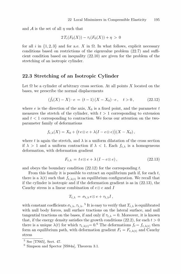
22 Local Minimizers in Compressible Elasticity 195
and A is the set of all η such that
2 Ti(F0(X)) − τi(F0(X)) + η > 0
for all i in 1, 2, 3 and for a.e. X in Ω. In what follows, explicit necessaryconditions based on restrictions of the eigenvalue problem (22.7) and suffi-cient condition based on inequality (22.10) are given for the problem of thestretching of an isotropic cylinder.
22.3 Stretching of an Isotropic Cylinder
Let Ω be a cylinder of arbitrary cross section. At all points X located on thebases, we prescribe the normal displacements
(ft(X) −X) · e = (t− 1) (X −X0) · e , t > 0 , (22.12)
where e is the direction of the axis, X0 is a fixed point, and the parameter tmeasures the stretch of the cylinder, with t > 1 corresponding to extensionand t < 1 corresponding to contraction. We focus our attention on the two-parameter family of deformations
ft,λ(X) = X0 +(t e⊗ e+ λ(I − e⊗ e)
)(X −X0) ,
where t is again the stretch, and λ is a uniform dilatation of the cross sectionif λ > 1 and a uniform contraction if λ < 1. Each ft,λ is a homogeneousdeformation, with deformation gradient
Ft,λ = t e⊗ e+ λ (I − e⊗ e) , (22.13)
and obeys the boundary condition (22.12) for the corresponding t.From this family it is possible to extract an equilibrium path if, for each t,
there is a λ(t) such that ft,λ(t) is an equilibrium configuration. We recall thatif the cylinder is isotropic and if the deformation gradient is as in (22.13), theCauchy stress is a linear combination of e⊗ e and I
Tt,λ = σt,λ e⊗ e+ τt,λI ,
with constant coefficients σt,λ, τt,λ. 5 It is easy to verify that Tt,λ is equilibratedwith null body forces, null surface tractions on the lateral surface, and nulltangential tractions on the bases, if and only if τt,λ = 0. Moreover, it is knownthat, if the energy density satisfies the growth conditions (22.2), for each t > 0there is a unique λ(t) for which τt,λ(t)= 0.6 The deformations ft = ft,λ(t) thenform an equilibrium path, with deformation gradient Ft = Ft,λ(t) and Cauchystress
5 See [TN65], Sect. 47.6 Simpson and Spector [SS84a], Theorem 3.1.

196 G. Del Piero and R. Rizzoni
Tt = σt e⊗ e , σt = σt,λ(t) . (22.14)
Assume that the configuration ft with t = 1 is a local minimizer. Then thethe minimizing interval from ft is the largest interval (ta, tb) with ta ≤ 1 ≤ tb,in which all eigenvalues of problem (22.7) are positive. An upper bound forta and a lower bound for tb are obtained from inequality (22.9), where nowcT = min σt, 0 = −σ−
t due to (22.14), and c sC = c s
C(Ft) due to the fact thatthe deformation is homogeneous. The inequality then takes the form
csC(Ft) > cK,t σ−
t . (22.15)
For the local condition (22.10), it is proved in [DR07] that it takes the sameform as (22.15), with cKT replaced by
c∗K,t = 1
2 cK,t + (cK,t − 1)1/2.
In particular, all configurations Ft with σ−t = 0 are minimizing configurations
if Cs(Ft) is positive definite. The absence of bifurcation in tension observed
by several authors in various circumstances7 is then, in fact, a property of allmaterials for which C
s is positive definite.As a specific example, we consider a Blatz–Ko material, whose energy
density isw(F ) = α
(12 (F · F − 3) + γ−1((detF )−γ − 1)
),
with α and γ positive constants. For it, we find that the equilibrium conditionτt,λ(t) = 0 is satisfied by
λ(t) = t1−δ/2 , δ = 2+3γ1+γ . (22.16)
For ft = ft,λ(t), we have
Ft = t e⊗ e+ t1−δ/2(I − e⊗ e) , detFt = t3−δ , (22.17)
and after some computation, we find that
σt = α t−1(tδ − 1
), csC(Ft) = 2α t−1.
We observe that σt is positive for t > 1 and negative for t < 1, and that csC(Ft)is positive for all t > 0. Then inequality (22.15) is always verified in tension,and the upper extreme of the minimizing interval is tb = +∞. In compression,the same inequality takes the form 2 > cK,t (1 − tδ). An upper bound for thelower extreme ta of the minimizing interval is then provided by the equation
cK,t (1 − tδ) = 2 . (22.18)
This equation always admits solutions in (0,1). Indeed, it is generally truethat cK,t ≥ 2, the value 2 being attained only if ∂1Ω = ∂Ω. Then the left-hand
7 See [Sp84] and the papers cited therein.

22 Local Minimizers in Compressible Elasticity 197
side of (22.18) is not less than 2 for t = 0 and is zero for t = 1. Because cK,t
depends continuously on t, the value 2 must be attained somewhere in (0,1).The same equation with cK,t replaced by c∗
K,t provides the upper bound forta according to the local condition (22.10). Since c∗
K,t > cK,t for all cK,t > 2,one sees that the new bound improves the one provided by equation (22.18).
22.4 Numerical Results for Circular Cylinders
In this section, we give some estimates for circular cylinders made of a Blatz–Ko material. Since for such a material the minimizing intervals are of the form(ta,+∞), our task reduces to finding upper and lower bounds for ta.
Let Ω be a circular cylinder of height H1 and radius R1, and let t → ft bethe equilibrium path (22.17). Then every ft is a map of Ω into the cylinderωt of height Ht = tH1 and radius Rt = t1−δ/2R1. To get a lower bound for ta,for each t we evaluate the smallest eigenvalue of problem (22.7) restricted tosuitable subspaces of W 1,∞(ωt). In particular, we take two subspaces made ofall functions u of the form 8
u =
⎧⎪⎨⎪⎩
x1ϕ(r) cos nπx3
Ht
x2ϕ(r) cos nπx3
Ht
ψ(r) sin nπx3
Ht
⎫⎪⎬⎪⎭, u =
⎧⎪⎨⎪⎩
0
ϕ(x2) cos nπx3
Ht
ψ(x2) sin nπx3
Ht
⎫⎪⎬⎪⎭, (22.19)
where n is an integer, O, x1, x2, x3 is a Cartesian coordinate system withorigin O at the center of one of the bases of the cylinder, x3 is the directionof the axis, r = (x2
1 + x22)
1/2 is the distance from the axis, and ϕ and ψ arefunctions in W 1,∞(−Rt, Rt). The functions u in the first subspace representdisplacements of the barreling type, whereas those in the second subspace rep-resent displacements of the buckling type in the (x2, x3) plane. The functionsof the first type are required to obey the regularity conditions at the origin
ϕ(0) = 0 , (rϕ′)(0) = 0 ,
and those of the second type are restricted by the normalization conditions
ϕ(0) = 1 , ψ(0) = 0 .
Both satisfy the boundary condition (22.12). The condition div(B(F0)
)= 0
reduces to the system of differential equations
(2 + γ)(rϕ′′ + 3ϕ′) + (1 + γ)nπHt
ψ′ − tδ n2π2
H2trϕ = 0,
rψ′′ + ψ′ − (1 + γ)nπHt
(r2ϕ′ + 2 rϕ) − (1 + γ + tδ) n2π2
H2trψ = 0
(22.20)
8 The lower bounds corresponding to functions of the barreling type were deter-mined in [SS84a] and [SS84b], and those corresponding to functions of the buck-ling type were determined in [DR07].
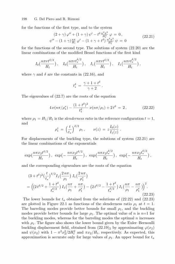
198 G. Del Piero and R. Rizzoni
for the functions of the first type, and to the system
(2 + γ)ϕ′′ + (1 + γ)ψ′ − tδ n2π2
H2tϕ = 0 ,
ψ′′ − (1 + γ)nπHt
ϕ′ − (1 + γ + tδ) n2π2
H2tψ = 0
(22.21)
for the functions of the second type. The solutions of system (22.20) are thelinear combinations of the modified Bessel functions of the first kind
I0(nπrtδ/2
Ht
), I0
(nπrtδ/2∗
Ht
), I1
(nπrtδ/2
Ht
), I1
(nπrtδ/2∗
Ht
),
where γ and δ are the constants in (22.16), and
tδ∗ =γ + 1 + tδ
γ + 2.
The eigenvalues of (22.7) are the roots of the equation
4 ν(nπ/ρ∗1) −
(1 + tδ)2
tδ∗ν(nπ/ρ1) + 2 tδ = 2 , (22.22)
where ρ1 = H1/R1 is the slenderness ratio in the reference configuration t = 1,and
ρ∗1 =
( t
t∗
)δ/2
ρ1 , ν(z) = zI0(z)
I1(z).
For displacements of the buckling type, the solutions of system (22.21) arethe linear combinations of the exponentials
exp(nπx2t
δ/2
Ht
), exp
(− nπx2t
δ/2
Ht
), exp
(nπx2tδ/2∗
Ht
), exp
(− nπx2t
δ/2∗
Ht
),
and the corresponding eigenvalues are the roots of the equation
(3 + tδ)2( tt∗
)δ/2I1
(2nπ
ρ1
)I1
(2nπ
ρ∗1
)
=((
2 tδ/2 +1 + tδ
tδ/2∗
)I1
(nπρ1
+nπ
ρ∗1
)−
(2 tδ/2 − 1 + tδ
tδ/2∗
)I1
(nπρ1
− nπ
ρ∗1
))2
.
(22.23)The lower bounds for ta obtained from the solutions of (22.22) and (22.23)
are plotted in Figure 22.1 as functions of the slenderness ratio ρ1 at t = 1.The barreling modes provide better bounds for small ρ1, and the bucklingmodes provide better bounds for large ρ1. The optimal value of n is n=1 forthe buckling modes, whereas for the barreling modes the optimal n increaseswith ρ1. The figure also shows the lower bound given by the Euler–Bernoullibuckling displacement field, obtained from (22.19)2 by approximating ϕ(x2)and ψ(x2) with 1 − π2x2
2/2H2t and πx2/Ht, respectively. As expected, this
approximation is accurate only for large values of ρ1. An upper bound for ta

22 Local Minimizers in Compressible Elasticity 199
Fig. 22.1. Upper and lower bounds for the compressive stretching ta for circularcylinders made of a Blatz–Ko material.
is provided by (22.18) with cK,t replaced by c∗K,t. In it, a major problem is the
determination of the exact value, or at least of an upper bound, for the Kornconstant cK appearing in the expression (22.11) of cK,t. This is still an openproblem. We use Bernstein and Toupin’s approximated formula [BT60]9
cK ≈ 2 +4 Jmax
Jmed + Jmin,
in which Jmax ≥ Jmed ≥ Jmin are the principal moments of inertia of thecylinder. For a circular cylinder with slenderness ratio ρt = Ht/Rt = tδ/2ρ1,one has
cK,t ≈ 2 + max 12
3 + tδρ21
,2
3tδρ2
1
,
and substituting into (22.18), one finds that an approximate upper bound forta is provided by the solutions of
ρ 21 t 2δ+ 9 t δ = 6 for ρ2
1 < 6 , ρ 21 (1 − t δ) = 3 for ρ2
1 > 6 ,
the approximation being due to the uncertainty about the expression used forthe Korn constant. This bound is represented by a curve in Figure 22.1. Forcomparison, the same figure also shows the estimate given in [Be71], obtained
9 This is neither an upper bound nor a lower bound for cK . It is not an upperbound because it is obtained solving a minimum problem over a strict subclassof the admissible deformation gradient fields, and it is not a lower bound becauseit refers to boundary conditions less restrictive than (22.12).

200 G. Del Piero and R. Rizzoni
using the Bernstein and Toupin approximation for the Korn constant, and aless refined expression for the constant cK,t.
We see that the two curves representing the overall upper and (approxi-mate) lower bounds are similar in shape, since both consist of two segments,one corresponding, roughly, to deformations of the buckling type and one cor-responding to deformations of the barreling type. The gap between the twocurves, as it comes from the results available in the literature (light gray areain Figure 22.1) has been substantially reduced by the present study (dark grayarea). The gap is narrow for large values of ρ1 but still important for small val-ues. This reveals the need for a deeper study of the minimizing displacementmodes for thick cylinders.
Acknowledgement. This work has been supported by PRIN 2005 “Modelli Matem-atici per la Scienza dei Materiali” and by the Research Project “Nano & Nano” ofthe University of Ferrara.
References
[Be71] Beatty, M.F.: Estimation of ultimate safe loads in elastic stability theory.J. Elasticity, 1, 95–120 (1971).
[BT60] Bernstein, B., Toupin, R.A.: Korn inequalities for the sphere and the circle.Arch. Rational Mech. Anal., 6, 51–64 (1960).
[Dp80] Del Piero, G.: Lower bounds for the critical loads of elastic bodies, J.Elasticity, 10, 135–143 (1980).
[DR07] Del Piero, G., Rizzoni, R.: Weak local minimizers in finite elasticity (inpreparation).
[GH95] Giaquinta, M., Hildebrandt, S.: Calculus of Variations. Springer, Berlin-Heidelberg (1996).
[Ho64] Holden, J.T.: Estimation of critical loads in elastic stability theory. Arch.Rational Mech. Anal., 17, 171–183 (1964).
[SS84a] Simpson, H.C., Spector, S.J.: On barrelling instabilities in finite elasticity,J. Elasticity, 14, 103–125 (1984).
[SS84b] Simpson, H.C., Spector, S.J.: On barrelling for a special material in finiteelasticity. Quart. Appl. Math., 42, 99–111 (1984).
[Sp84] Spector, S.J.: On the absence of bifurcation for elastic bars under tension.Arch. Rational Mech. Anal., 85, 171–199 (1984).
[TN65] Truesdell, C., Noll, W.: The Non-Linear Field Theories of Mechanics. In:Flugge, S. (ed.), Handbuch der Physik, III/3. Springer, Berlin-Heidelberg-New York (1965).

23
Harmonic Oscillations in a Linear Theory ofAntiplane Elasticity with Microstructure
S. Potapenko
University of Waterloo, ON, Canada; [email protected]
23.1 Introduction
The theory of micropolar (Cosserat) elasticity [Er66] has been developed toaccount for discrepancies between the classical theory and experiments whenthe effects of material microstructure were known to affect significantly thebody’s overall deformation, for example, in the case of granular bodies withlarge molecules (e.g., polymers) or human bones (see [Lak95], [Lak91], and[Lak82]). Significant progress has been achieved in this direction for the last 30years (see [Now86] for a review of works in this area and an extensive bibliog-raphy), but investigations have been confined mainly to the problems of elas-tostatics. A dynamic problem of wave propagation in the three-dimensionalelastic micropolar space was formulated by Kupradze in [Kup79]. However, arigorous treatment of the corresponding boundary value problems in the an-tiplane case when waves propagate in an infinite cylinder of any arbitrary crosssection in the direction of the generators of the cylinder or in the unboundedantiplane space is, to the author’s knowledge, still absent from the litera-ture. The main difficulties arising here are when we try to apply Helmholtz’stheorem to a solution of the governing equations in the exterior domain. Thedecomposition is not as straightforward as in classical elasticity. Only one partsatisfies a Helmholtz equation, and so we can impose only one Sommerfeld-type radiation condition.
In this chapter, we introduce time dependency into the theory of antiplanemicropolar elasticity presented in [PSM05] by considering the case where allapplied forces, and hence, displacement, strain, and stress components areperiodic functions of time. Furthermore, we find that uniqueness is guaranteed,provided that the frequency of oscillation is greater than a fixed constantmultiple of the speed of longitudinal waves in an infinite micropolar medium.

202 S. Potapenko
23.2 Preliminaries
In what follows, Greek and Latin indices take the values 1,2 and 1,2,3, respec-tively, the convention of summation over repeated indices is understood, anda superscript T indicates matrix transposition.
Let S be a domain in R2 bounded by a closed C2-curve ∂S and occupied by
a homogeneous and isotropic linearly elastic micropolar material with elasticconstants λ, µ, α, β, γ, and κ. The state of micropolar antiplane shear is char-acterized by a displacement field U (x′, t) = (U1 (x′, t) , U2 (x′, t) , U3 (x′, t))T
and a microrotation field φ (x′, t) = (φ1 (x′, t) , φ2 (x′, t) , φ3 (x′, t))T of theform Uα (x′, t) = 0, U3(x
′, t) = U3 (x, t) , φ3 (x′, t) = 0, φα(x′, t) = φα (x, t) ,where x′ = (x1, x2, x3) and x = (x1, x2) are generic points in R
3 and R2,
respectively. In the absence of body forces and moments, we find that theequations of motion of micropolar antiplane shear written in terms of dis-placements and microrotations are
L(∂x)U(x, t) = F (x, t), x ∈ S, (23.1)
Here U(x, t) = (U1(x, t), U2(x, t), U3(x, t))T , where the Uα have replaced theφα, and the matrix partial differential operator L(∂x) = L (∂/∂xα) is definedby
L (ξ) = L (ξα)
=
⎛⎝
(γ + κ)∆ − 4α + (β + γ − κ)ξ21 (β + γ − κ)ξ1ξ2 2αξ2
(β + γ − κ)ξ1ξ2 (γ + κ)∆ − 4α + (β + γ − κ)ξ22 −2αξ1
−2αξ2 2αξ1 (µ + α)∆
⎞⎠,
with ∆ = ξαξα.Together with L, we consider the boundary stress operator T (∂x) =
T (∂/∂xα) defined by
T (ξ) = T (ξα)
=
⎛⎝
(2γ + β) ξ1n1 + (γ + κ) ξ2n2 (γ − κ)ξ2n1 + βξ1n2 2αn2
(γ − κ)ξ1n2 + βξ2n1 (γ + κ) ξ1n1 + (2γ + β) ξ2n2 2αn1
0 0 (µ + α)ξαnα
⎞⎠,
where n = (n1, n2)T is the unit outward normal to ∂S,
F (x, t) =
(J
∂2U1
∂t2, J
∂2U2
∂t2, ρ
∂2U3
∂t2
)T
,
ρ is the mass density, and J is the moment of inertia.Furthermore, we assume that the time dependency is periodic, that is, the
waves are monochromatic; consequently, U(x, t) may be represented in theform

23 Harmonic Oscillations in Antiplane Elasticity 203
U(x, t) = Re[u(x)e−iωt], (23.2)
where ω ∈ R is the frequency of oscillation and u(x) = (u1(x), u2(x), u3(x))T
is some real-valued function.Substituting (23.2) in (23.1), we find that in terms of u(x) = (u1, u2, u3)
T ,system (23.1) becomes
⎡⎣L(∂x) +
⎛⎝Jω2 0 00 Jω2 00 0 ρω2
⎞⎠⎤⎦u(x) = 0. (23.3)
Throughout what follows, we assume the following restrictions on the elas-tic constants of the material [PSM05]:
2γ + β > 0, κ, α, γ, µ > 0. (23.4)
23.3 Expansion of a Regular Solution
To obtain the analytical solution of (23.3), we have to prove the followingtheorem.
Theorem 1. Any regular solution of system (23.3) admits in the domain ofregularity a representation
u(x) =
(∂Φ
∂x1− ∂Ψ
∂x2,∂Φ
∂x2+
∂Ψ
∂x1, u3
)
such that(∆+ k2
1)(∆+ k22)Ψ = 0 (i),
(∆+ k21)(∆+ k2
2)u3 = 0 (ii),(∆+ k2
3)Φ = 0 (iii),
wherek21 + k2
2 = 4α2+Jω2−4α+ρω2(γ+ε)(µ+α)(γ+ε) ,
k21k
22 = ρω2(Jω2−4α)
(µ+α)(γ+ε) , k23 = (Jω2−4α)
2γ+β .
This assertion can be proved by direct verification, following the procedurediscussed in [SC93].
23.4 Radiation Conditions
Let S+ ≡ S and S− ≡ R2\(S+ ∪ ∂S). We now consider solutions of (23.3) inthe domain S−. Clearly, since the domain of interest now extends to infinity,we must consider the behavior of any solution of (23.3) at infinity.
In the history of uniqueness theorems for oscillation problems, a impor-tant role was played by the Sommerfeld-type radiation conditions for the

204 S. Potapenko
Helmholtz equation. They were later generalized for the elastodynamic prob-lem by Kupradze [Kup65]. To proceed, we establish suitable radiation condi-tions and asymptotic estimates for the functions Ψ(x), Φ(x), and u3(x).
Definition 1. Let x ∈ S−. If, as |x| = R → ∞,
Ψ(x) = o(R−1/2),∂Ψ
∂xα(x) = O(R−1), (23.5)
Φ(x) = O(R−1/2),∂Φ
∂R(x) − ik3Φ(x) = o(R−1/2), (23.6)
u3(x) = o(R−1/2),∂u3
∂xα(x) = O(R−1), (23.7)
we say that the regular solution u(x) = ( ∂Φ∂x1
− ∂Ψ∂x2
, ∂Φ∂x2
+ ∂Ψ∂x1
, u3) satisfies theradiation conditions.
23.5 Boundary Value Problems
Let f and g be continuous (3 × 1) matrices prescribed on ∂S. Consider thefollowing Dirichlet and Neumann boundary value problems in the exteriordomain S−.
(D−) Find a regular solution u of (23.3) in the domain S−, satisfying theradiation conditions (23.5)–(23.7) and the boundary condition
u(x) = f(x), x ∈ ∂S.
(N−) Find a regular solution u of (23.3) in the domain S− satisfying theradiation conditions (23.5)–(23.7) and the boundary condition
T (∂x, n)u(x) = g(x), x ∈ ∂S,
where n is the unit outward normal to ∂S.
23.6 Uniqueness Theorem
Theorem 2. If ω2 > 4α/J , then (D−) and (N−) have at most one solution.
Proof. To verify this, it is enough to show that in the case of homogeneousDirichlet or Neumann boundary conditions the solution is identically zero.Consider system (23.3). As stated above, it is clear that finding an analyticalsolution to (23.3) is equivalent to determining functions Φ and Ψ that satisfy(23.4).
Let Ω = (∆+k22)Ψ. Then, by Theorem 1(i), (∆+k2
1)Ψ = 0 in S−. Considerthe integral

23 Harmonic Oscillations in Antiplane Elasticity 205
∫
∂KR
|Ω|2 dS,
where ∂KR is the circumference of a circle, radius R, sufficiently large toenclose ∂S. Using the asymptotic estimates (23.5) for Ψ , it is a straightforwardexercise to show that
limR→∞
∫
∂KR
|Ω|2 dS = 0. (23.8)
Since Ω solves a Helmholtz equation with k21 > 0, we can use (23.8) and
Rellich’s lemma citeKupradze2 to deduce that Ω = 0 in S−; that is,
(∆ + k22)Ψ = 0 in S−.
As above, (23.5) gives us that
limR→∞
∫
∂KR
|Ψ |2 dS = 0.
Rellich’s Lemma with k22 > 0 then leads us to
Ψ = 0 in S−. (23.9)
Similarly, starting from (ii), we obtain
u3 = 0 in S−. (23.10)
Applying the reciprocity relation for the elastostatic antiplane shear deforma-tions of Cosserat solids [PSM05] to a regular solution of (23.3) in the boundedregion S− ∩ KR, we obtain
∫
∂S+KR
[uT Tu − uT Tu
]dS = 0. (23.11)
Next, following standard procedures for uniqueness proofs in the theory ofboundary value problems, we impose zero Dirichlet or Neumann conditionson ∂S, so that (23.11) becomes
∫
KR
[uT Tu − uT Tu
]dS = 0. (23.12)
Furthermore, substituting the representation of u(x) given in Theorem 1 into(23.12), taking into account (23.6) and the conditions (23.4) imposed on theelastic constants, and following exactly the procedure described in [SC93] toprove the uniqueness theorems for oscillations of plates, we obtain, as R → ∞,
limR→∞
∫
∂KR
|Φ|2 dS = 0. (23.13)
Theorem 1(ii), (23.13), and Rellich’s lemma now imply that

206 S. Potapenko
Φ = 0 in S−. (23.14)
Hence, in view of (23.9), (23.10), and (23.14),
u(x) = 0 in S−,
which completes the proof.
Remark 1. The condition ω2 > 4α/J is necessary to ensure that k2i > 0 and
hence the use of Rellich’s Lemma.
References
[Er66] Eringen, A.C.: Linear theory of micropolar elasticity. J. Math. Mech., 15,909–923 (1966).
[Kup65] Kupradze, V.D.: Potential Methods in the Theory of Elasticity. Israel Pro-gram for Scientific Translations, Jerusalem (1965).
[Kup79] Kupradze, V.D., Gegelia, T.G., Basheleishvili, M.O., Burchuladze, T.V.:Three-Dimensional Problems of the Mathematical Theory of Elasticity andThermoelasticity. North-Holland, Amsterdam (1979).
[Lak82] Lakes, R.: Dynamical study of couple stress effects in human compactbone. J. Biomedical Engng., 104, 6–11 (1982).
[Lak91] Lakes, R.: Experimental micromechanics methods for conventional andnegative Poisson’s ratio cellular solids as Cosserat continua. J. Engng.Materials Tech., 113, 148–155 (1991).
[Lak95] Lakes, R.: Experimental methods for study of Cosserat elastic solids andother generalized elastic continua. In: Muhlhaus, H-B. (ed.), ContinuumModels for Materials with Microstructure. Wiley, New York (1995), pp.1–22.
[Now86] Nowacki, W.: Theory of Asymmetric Elasticity. Polish Scientific Publish-ers, Warszawa (1986).
[PSM05] Potapenko, S., Schiavone, P., Mioduchowski, A.: Anti-plane shear defor-mations in a linear theory of elasticity with microstructure. J. Appl. Math.Phys. (ZAMP), 56, 516–528 (2005).
[SC93] Schiavone, P., Constanda, C.: Oscillation problems in thin plates withtransverse shear deformation. SIAM J. Appl. Math., 53, 1253–1263(1993).

24
Exterior Dirichlet and Neumann Problems forthe Helmholtz Equation as Limits ofTransmission Problems
M.-L. Rapun1 and F.-J. Sayas2
1 Universidad Politecnica de Madrid, Spain; [email protected] Universidad de Zaragoza, Spain; [email protected]
24.1 Statement of the Problems
In this chapter, we propose a new way of understanding the classical exte-rior Dirichlet and Neumann problems for the Helmholtz equation as limitingsituations of transmission problems, and study the stability of this limitingprocess under discretization. This kind of problems appear in the study of thescattering of time-harmonic acoustic and thermal waves.
We assume that Ωint ⊂ Rd, d = 2 or 3, is a bounded, simply connected,
open set with smooth boundary Γ . If the obstacle is impenetrable, then thescattering amplitude of a time-harmonic wave with wavenumber λ2 solvesan exterior Dirichlet or Neumann problem for the Helmholtz equation ∆u +λ2u = 0 in Ωext := R
d \ Ωint. It satisfies the Sommerfeld radiation conditionat infinity
limr→∞
rd−12 (∂ru − ıλu) = 0,
uniformly in all directions x/|x| ∈ Rd, r := |x| (see [CK83]). When waves can
propagate through Γ , that is, when the obstacle is penetrable, and the physicalproperties in both media are different, the problem in Ωint is modeled by∆u + µ2u = 0. Both Helmholtz equations are coupled through two continuityconditions of the form
uint − uext = f, on Γ ,
α ∂nuint − β ∂nuext = β g, on Γ .
Typically, f = uinc and g = ∂nuinc are the Cauchy data on Γ of an incidentwave, a known solution to the exterior Helmholtz equation. In acoustics, µ2 isproportional to ρ/α2, where ρ is the density and α the velocity of transmissionin Ωint. For thermal waves, µ2 is proportional to ıρ/α, where ρ is the densitymultiplied by the specific heat capacity and α is the conductivity. Generalconditions on the parameters λ, µ, α, and β guaranteeing uniqueness can befound in [RS06a] and the references therein.

208 M.-L. Rapun and F.-J. Sayas
Dirichlet, Neumann, and transmission problems have been studied suc-cessfully from both the analytical and the numerical points of view in a widenumber of works with a special emphasis on the study of acoustic waves (seefor instance [CK83], [CS85], [KM88], [KR78], and [TW93]). More recently,Helmholtz transmission problems have also appeared in the study of scatter-ing of thermal waves (see [Man01], [RS06a], and [TSS02]).
When studying the behavior of the solution to the transmission problemdepending on the interior parameters, physical experiments as well as numeri-cal simulations seem to point out that, for a fixed interior wave number, whenthe parameter α tends to zero, the solution to
(Pα)
∣∣∣∣∣∣∣∣∣∣∣∣∣∣
∆uα + λ2uα = 0, in Ωext,
∆uα + µ2uα = 0, in Ωint,
uintα − uext
α = f, on Γ ,
α ∂nuintα − β ∂nuext
α = β g, , on Γ ,
limr→∞
rd−12 (∂ruα − ıλuα) = 0,
tends to the solution to the exterior Neumann problem
(PN )
∣∣∣∣∣∣∣∣
∆uN + λ2uN = 0, in Ωext,
∂nuN = −g, on Γ ,
limr→∞
rd−12 (∂ruN − ıλuN ) = 0,
whereas if α goes to infinity, the solution (Pα) converges to the solution of theexterior Dirichlet problem
(PD)
∣∣∣∣∣∣∣∣
∆uD + λ2uD = 0, in Ωext,
uD = −f, on Γ ,
limr→∞
rd−12 (∂ruD − ıλuD) = 0.
This can also be seen by taking limits formally. The aim of this work is togive a rigorous proof of these facts, providing the corresponding convergencerates. We want to point out that we are restricting ourselves to a particularfamily of transmission problems where only one of the two interior parametersvaries. In this case we will show linear convergence. To improve our estimates,both interior parameters would have to converge to zero in the Neumann caseor to infinity in the Dirichlet one. In view of numerical experiments in thetwo-dimensional setting, we believe that for the case of the Dirichlet problem,the faster the modulus of the interior wavenumber increases, the higher theconvergence rate is, although we cannot predict any rate in terms of it. On theother hand, for the Neumann problem, we have not observed any substantialimprovement by making the interior wavenumber tend to zero. At the current

24 Dirichlet and Neumann Problems as Limits of Transmission Problems 209
stage of our research, we cannot prove the results when both parameters vary,since our study is based on the very simple fact that all the integral operatorsinvolved in the boundary formulation do not depend on α. Taking into accountthat the fundamental solution depends on the wavenumber, our study cannotbe adapted easily to the case of a family of transmission problems dependingon both interior parameters.
24.2 Boundary Integral Formulations
Since we are dealing with exterior problems, a suitable way of inspecting themis by using boundary integral formulations. We introduce the fundamentalsolution to the Helmholtz equation ∆u + ρ2u = 0,
φρ(x,y) :=
ıH
(1)0 (ρ |x − y|)/4, if d = 2,
exp(ı ρ|x − y|)/(4π|x − y|), if d = 3,
and the single-layer potential
Sρϕ :=∫
Γφρ( · ,y)ϕ(y) dγy : R
d −→ C.
We also define the boundary integral operators
V ρϕ :=∫
Γφρ( · ,y)ϕ(y) dγy : Γ −→ C,
Jρϕ :=∫
Γ∂n( · )φρ( · ,y)ϕ(y) dγy : Γ −→ C.
We recall some well-known properties of the integral operators above (see[McL00]): (i) the bounded operator V ρ : H−1/2(Γ ) → H1/2(Γ ) is invertible ifand only if −ρ2 is not a Dirichlet eigenvalue of the Laplace operator in Ωint;(ii) the bounded operator − 1
2I + Jρ : H−1/2(Γ ) → H−1/2(Γ ) is invertible;
and (iii) the bounded operator 12I + Jρ : H−1/2(Γ ) → H−1/2(Γ ) is invertible
if and only if −ρ2 is not a Neumann eigenvalue of the Laplace operator inΩint.
We will use indirect formulations in terms of single-layer potentials thatcan fail if either −µ2 or −λ2 are Dirichlet eigenvalues of the Laplace operatorin Ωint and if −µ2 is a Neumann eigenvalue of the Laplacian in Ωint. To avoidthese particular cases, we can adapt our results to the indirect formulationproposed in [RS06b] and based on Brakhage–Werner potentials.
The solution to the Dirichlet problem (PD) can be represented as uD =SλψD, where ψD is the unique solution to
V λψD = −f. (24.1)
The solution to the Neumann problem (PN ) is uN = SλψN , where ψN is theunique solution to

210 M.-L. Rapun and F.-J. Sayas
( 12I − Jλ)ψN = g. (24.2)
Finally, the solution to the transmission problem (Pα) can be obtained asuα = Sλψα in Ωext and uα = Sµϕα in Ωint, with (ψα, ϕα) solving
Hα
[ϕα
ψα
]:=
[V µ −V λ
α( 12I + Jµ) β( 1
2I − Jλ)
][ϕα
ψα
]=
[f
β g
]. (24.3)
The proof of these results can be found in [CZ92, Chap. 7] and [RS06a].
24.3 Convergence Analysis
We start by noticing that if x ∈ Ωext, then
|uα(x)−u∗(x)| = |Sλ(ψα−ψ∗)(x)| = |〈ψα−ψ∗, φλ(x, · )〉| ≤ Cx‖ψα−ψ∗‖−1/2,
where the subscript “∗” stands for either D or N . Therefore, the study ofpointwise convergence in Ωext can be carried out by analyzing the convergenceof the densities in H−1/2(Γ ). Indeed, here we use the natural H−1/2(Γ )-norm,but when using a weaker or stronger norm, one obtains the same convergencerate in terms of α. The only difference is the constant appearing in the esti-mate. In any case, it does not depend on α, but depends on x. It only blowsup when we are close to Γ and it is uniformly bounded in the exterior of anyball containing Γ when λ ∈ R, whereas for λ ∈ R, uniform boundedness isonly assured in compact sets.
Proposition 1. Consider the operators
A := (12I + Jµ)(V µ)−1 : H1/2(Γ ) → H−1/2(Γ ),
D := β−1( 12I − Jλ)−1AV λ : H−1/2(Γ ) → H−1/2(Γ ),
Hα := β( 12I − Jλ) + αAV λ : H−1/2(Γ ) → H−1/2(Γ ).
Then
(a) If |α| < ‖D‖−1, then Hα is invertible. Moreover,
‖H−1α ‖ ≤ C, ∀ |α| ≤ α0 < ‖D‖−1.
(b) If |α| > ‖D−1‖, then Hα is invertible. Moreover,
‖H−1α ‖ ≤ C |α|−1, ∀ |α| ≥ α0 > ‖D−1‖.
(c) If either |α| < ‖D‖−1 or |α| > ‖D−1‖, then
ψα = H−1α (−αAf + β g) . (24.4)

24 Dirichlet and Neumann Problems as Limits of Transmission Problems 211
Proof. First, we assume that |α| < ‖D‖−1 and decompose
Hα = β( 12I − Jλ)(I + αD). (24.5)
Applying the geometric series theorem (see [AH01, Theorem 2.3.1]), we deducethat Hα is invertible. Furthermore, for all |α| ≤ α0 < ‖D‖−1,
‖H−1α ‖ ≤ ‖β−1( 1
2I − Jλ)−1‖‖(I + αD)−1‖ ≤ C
1 − |α|‖D‖ ≤ C ′.
For |α| > ‖D−1‖, the proof is completely analogous: We now decompose
Hα = αAV λ(I + α−1D−1), (24.6)
to deduce the invertibility of Hα and the uniform bound
‖H−1α ‖ ≤ |α|−1‖(V λ)−1A−1‖‖(I + α−1D−1)−1‖ ≤ C |α|−1
1−|α|−1‖D−1‖ ≤ C ′|α|−1,
for all |α| ≥ α0 > ‖D−1‖. Finally, to show (c), we remark that
Hα =
[I 0
αA I
][V µ −V λ
0 Hα
],
with Hα being the operator introduced in (24.3). By (a) and (b), the operatorHα is invertible for the considered values of α, and
H−1α =
[(V µ)−1 (V µ)−1V λH−1
α
0 H−1α
][I 0
−αA I
]
=
[(V µ)−1(I − αV λH−1
α A) (V µ)−1V λ H−1α
−α H−1α A H−1
α
].
Finally, the result follows readily from (24.3).
Proposition 2. (a) For all |α| ≤ α0 < ‖D‖−1 ,
‖ψα − ψN‖−1/2 ≤ C |α|.
(b) For all |α| ≥ α0 > ‖D−1‖ ,
‖ψα − ψD‖−1/2 ≤ C |α|−1.
Proof. (a) From (24.2) and (24.4) it follows that
ψα − ψN = −α H−1α Af +
(β H−1
α − ( 12I − Jλ)−1
)g,
and, by (24.5), we can write

212 M.-L. Rapun and F.-J. Sayas
β H−1α − ( 1
2I − Jλ)−1 = β H−1α − β(I + αD)H−1
α = −αβDH−1α .
Applying Proposition1(a), we now easily deduce the result. To prove (b), weproceed likewise: by direct computation using (24.1) and (24.4), we see that
ψα − ψD =(−αH−1
α A + (V λ)−1)f + βH−1
α g,
and, by (24.6), we have
−αH−1α A + (V λ)−1 = −αH−1
α A + (α I + D−1)H−1α A = D−1H−1
α A.
The result is now a consequence of Proposition1(b).
Corollary 1. (a) The solution of (Pα) converges to the solution of (PN ) inΩext as α → 0. Moreover, for all |α| ≤ α0 < 1/‖D‖,
|uα(x) − uN (x)| ≤ Cx|α|, x ∈ Ωext.
(b) The solution of (Pα) converges to the solution of (PD) in Ωext as α → ∞.Moreover, for all |α| ≥ α0 > ‖D−1‖,
|uα(x) − uD(x)| ≤ Cx|α|−1, x ∈ Ωext.
24.4 Convergence at the Discrete Level
In this section, we describe briefly how the previous study applies when dealingwith numerical approximations to (PD), (PN ), and (Pα) obtained by an ab-stract class of discretizations sharing some common features. The hypotheseswe will specify shortly are satisfied by a wide number of numerical methods;in particular, all the abstract Petrov–Galerkin schemes analyzed in [RS06a]fall into that setting, along with the quadrature methods studied in [DRS06].
We will assume that all the densities involved in the numerical solutionto the corresponding boundary integral equations are approximated in a dis-crete space Xm of dimension m. In principle, Xm could not be a subspaceof H−1/2(Γ ) as happens when using quadrature methods where the discretespace is formed by Dirac delta distributions. As in the continuous case, theconsidered norm does not add any difficulty as indicated at the beginning ofSection 24.3. We also assume that in order to compute the coordinates of theapproximate densities in a basis of Xm, one has to solve linear systems ofequations of the form
V λmψm
D = −fm, (24.7)
(12Im − Jλ
m)ψmN = gm, (24.8)
[V µ
m −V λm
α( 12Im + Jµ
m) β( 12Im − Jλ
m)
][ϕm
α
ψmα
]=
[fm
β gm
], (24.9)

24 Dirichlet and Neumann Problems as Limits of Transmission Problems 213
for (PD), (PN ), and (Pα), respectively, where the matrices V λm, Im, Jλ
m, V µm,
and Jµm do not depend on α. Obviously, to have a unique solution in (24.7)–
(24.9), the corresponding matrices have to be invertible. Then, with the samearguments as in Propositions 1 and 2, the following bounds can be proven:
‖ψα − ψN‖ ≤ C |α|, ∀ |α| ≤ α0,
‖ψα − ψD‖ ≤ C |α|−1, ∀ |α| ≥ α1,
where ‖ · ‖ is any norm in Cm. From here one deduces the same kind of
bounds for the densities in the norm of Xm. If the approximate solutions to(PD), (PN ), and (Pα) are defined by simply introducing the discrete densitiesobtained in (24.7)–(24.9) in the definition of the single-layer potentials, thenresults analogous to those in Corollary 1 can be derived straightforwardly.
24.5 Numerical Examples
This last section is devoted to numerical illustrations in the two-dimensionalsetting. The numerical method we use here is an easy-to-implement quadra-ture method proposed in [DRS06].
−2 −1.5 −1 −0.5 0 0.5 1 1.5−3
−2.5
−2
−1.5
−1
−0.5
0
Fig. 24.1. Geometry of the problem.
We have considered the nonconvex domain represented in Figure 24.1,whose boundary is smooth. The physical parameters are λ = µ = 1 + ı andβ = 1, which correspond to a problem of scattering of thermal waves. Wehave taken uinc(x1, x2) := exp(−ıλx2) as incident wave and have computedthe total wave
uinc + uα in Ωext, uα in Ωint,

214 M.-L. Rapun and F.-J. Sayas
for some different values of α. In Figure 24.2, we represent the modulus of thetotal wave for five transmission problems with decreasing values of α as wellas the modulus of the total wave that solves the exterior Neumann problem.Notice that the solution for α = 1 is the planar incident wave.
α = 1 α = 0.5 α = 0.25
α = 0.125 α = 0.0625 Neumann
Fig. 24.2. α = 1, 1/2, 1/4, 1/8, 1/16, and the Neumann exterior problem.
α = 1 α = 3 α = 9
α = 27 α = 81 Dirichlet
Fig. 24.3. α = 1, 3, 9, 27, 81, and the Dirichlet exterior problem.

24 Dirichlet and Neumann Problems as Limits of Transmission Problems 215
In Table 24.1, we write the errors ENabs := maxi |uα(xi) − uN (xi)| and
ENrel := maxi (|uα(xi)− uN (xi)|/|uN (xi)|), where xi are the 50× 50 points in
the rectangle [−2, 1.5]× [−3, 0] represented in Figure 24.1. The correspondingestimated convergence rates (ecr) are computed by comparing errors for con-secutive values of α in the usual way. It is clear that these numerical resultsfit with the theoretical ones.
We now solve the same problem for increasing values of α. In Figure 24.3,we represent the modulus of the total wave solution for the transmission andDirichlet problems. Relative and absolute errors at the points xi are written onthe right of Table 24.1. Notice that in this case, although absolute errors havealmost the same size as in the Neumann case, relative errors are now reallylarge. This is not surprising, since the total wave in the Dirichlet problem isalmost zero in the shadow of the obstacle.
Acknowledgement. The authors are partially supported by MEC/FEDER ProjectMTM-2004-01905, Gobierno de Navarra Project Ref. 18/2005, and by DGA-GrupoConsolidado PDIE.
Table 24.1. Absolute and relative errors for the Neumann and Dirichlet problems.
α ENabs ecr EN
rel ecr
10−1 5.95 ·10−2 1.24 ·10−1
10−2 6.33 ·10−3 0.97 1.34 ·10−2 0.9610−3 6.37 ·10−4 0.99 1.35 ·10−3 0.9910−4 6.37 ·10−5 0.99 1.35 ·10−4 0.9910−5 6.37 ·10−6 0.99 1.35 ·10−5 0.99
α EDabs ecr ED
rel ecr
101 2.30 ·10−1 5.00 ·102
102 2.77 ·10−2 -0.91 7.01 ·10 -0.85103 2.82 ·10−3 -0.99 7.25 -0.98104 2.82 ·10−4 -0.99 7.28 ·10−1 -0.99105 2.82 ·10−5 -0.99 7.28 ·10−2 -0.99
References
[AH01] Atkinson, K., Han, W.: Theoretical Numerical Analysis: A FunctionalAnalysis Framework. Springer, New York (2001).
[CZ92] Chen, G., Zhou, J.: Boundary Element Methods. Academic Press, London(1992).
[CK83] Colton, D.L., Kress, R.: Integral Equation Methods in Scattering Theory.Wiley, New York (1983).
[CS85] Costabel, M., Stephan, E.: A direct boundary integral equation methodfor transmission problems. J. Math. Anal. Appl., 106, 367–413 (1985).
[DRS06] Domınguez, V., Rapun, M.–L., Sayas, F.–J.: Dirac delta methods forHelmholtz transmission problems. Adv. Comput. Math. (in press).
[KM88] Kleinman, R.E., Martin, P.A.: On single integral equations for the trans-mission problem of acoustics. SIAM J. Appl. Math., 48, 307–325 (1988).

216 M.-L. Rapun and F.-J. Sayas
[KR78] Kress, R., Roach, G.F.: Transmission problems for the Helmholtz equa-tion. J. Math. Phys., 19, 1433–1437 (1978).
[Man01] Mandelis, A.: Diffusion–Wave Fields. Mathematical Methods and GreenFunctions. Springer, New York (2001).
[McL00] McLean, W.: Strongly Elliptic Systems and Boundary Integral Equations.Cambridge University Press, Cambridge (2000).
[RS06a] Rapun, M.-L., Sayas, F.-J.: Boundary integral approximation of a heatdiffusion problem in time-harmonic regime. Numer. Algorithms, 41, 127–160 (2006).
[RS06b] Rapun, M.-L., Sayas, F.-J.: Indirect methods with Brakhage–Werner po-tentials for Helmholtz transmission problems. In: Proceedings of ENU-MATH 2005. Springer, New York (2006), pp. 1146–1154.
[TSS02] Terron, J.M., Salazar, A., Sanchez–Lavega, A.: General solution for thethermal wave scattering in fiber composites. J. Appl. Phys., 91, 1087–1098(2002).
[TW93] Torres, R.H., Welland, G.V.: The Helmholtz equation and transmissionproblems with Lipschitz interfaces. Indiana Univ. Math. J., 42, 1457–1485(1993).

25
Direct Boundary Element Method withDiscretization of All Integral Operators
F.-J. Sayas
Universidad de Zaragoza, Spain; [email protected]
25.1 Introduction
The history of boundary element methods (BEMs) for elliptic boundary valueproblems is the result of a combination of many different approaches. The ori-gins of the method, from a purely theoretical point of view, can be traced backto the first studies of integral equations and, hence, to the birth of functionalanalysis. It was the development of Fredholm theory that first gave an impulseto numerical methods that reformulate a boundary value problem (BVP) onthe boundary of the domain and then solve an integral equation by any methodavailable. These first essays are centered on the use of integral equations ofthe second kind. Later on, when the ellipticity of some important boundaryintegral operators was proved, the type of boundary integral equation of inter-est changed drastically to integral equations of the first kind. In addition, theellipticity of the equations proved the adequacy of using Galerkin methods. Itwas back then that a main bifurcation happened between the mathematicaland the engineering literature on BEM. The gap is now much deeper than thewell-known duplication of efforts in the finite element world.
A priori, theorists in the mathematical community and some practitionersin the realm of physics have preferred boundary integral formulations thatlead to equations where Galerkin methods can be employed. In part becauseof the additional integration process that Galerkin methods impose, there hasbeen a preference for indirect formulations. In these, a potential is proposed asa solution of the partial differential equation. Imposition of boundary condi-tions leads to boundary integral equations. The unknown is a density withouta clear physical meaning, if it has any at all. On the side of advantages, equa-tions are simpler, data do not appear under the action of integral operatorsand there is a clear knowledge of how the numerical methods converge, withsome well-understood superconvergence phenomena in weak norms. However,in addition to the fact that we are computing something that has no physicalinterpretation (it is the numerical input of a function that gives the approx-

218 F.-J. Sayas
imate solution of the BVP), these equations fail to be well posed in somerelevant situations.
It has been advocated by the more practically-oriented community ofboundary element developers to insist in using direct formulations. These arisefrom taking Green’s third formula (actually, its adaptation to the particularelliptic operator) and substituting the data in it. Then the unknowns are theremaining Cauchy data. Even when the operator involved in the equation isnot invertible, the equation is always solvable and all possible solutions arevalid from the point of view of reconstructing the solution of the BVP. Weare nevertheless faced with having the data under the action of an integraloperator. Typically, practitioners have preferred collocation methods to par-tially compensate for this problem, even though there is no strong theoreticalsupport for their general convergence.
There is, however, an additional aspect of the practical literature on BEMthat is usually ignored by theorists. Even the most elementary texts treat theequations as if all the boundary data were unknown and discretizing all theintegral operators. Only in a final step, data are plugged into the equation.This approach further simplifies the need of approximating integrals in thepractical implementation of the method and makes these implementationsmore reusable for different boundary value problems.
In this paper we are going to explain, with a collection of very simpleexamples, how to profit from this idea in the context of Galerkin or Petrov-Galerkin methods. In some cases, we will construct methods that preprocessdata before inputting them in the discrete equations. In some other cases, wewill develop methods based on the theory of a mixed finite element method(FEM), where this projection of data and the computation of the unknownsare done simultaneously.
To fix the language of Petrov-Galerkin methods for operator equations (orvariational problems), we refer to Section 25.4, where we will shortly reviewsome important results. Proofs thereof, albeit in a very different language,can be found in [K99]. Results on inf-sup conditions and problems with mixedstructure can be found in [BF91]. For theoretical aspects on boundary inte-gral operators, we refer the reader to [M00] and its extensive bibliography. Avery thorough exposition of the basic theory of Sobolev spaces on Lipschitzboundaries can be found in the same monograph.
From among the many, and sometimes conflicting, notations for potentialsand integral operators, we will be using those of George Hsiao (see Section 25.2and [GH95], for example). The angled bracket 〈 · , · 〉 will be used to denotethe H−1/2(Γ ) × H1/2(Γ )-duality product that arises from identifying L2(Γ )with its dual space. The norm on Hr(Γ ) will be denoted simply by ‖ · ‖r.

25 Direct BEM with Discretization of All Operators 219
25.2 Model Problem, Potentials, and Operators
As a very simple model problem, where we can concentrate on the boundaryoperators avoiding some unimportant technicalities, we will consider Yukawa’sequation in an exterior domain. Let then Γ be the boundary of a Lipschitzdomain (connectedness of this domain is not necessary), and let Ω be theexterior of this domain. We then consider the problem
u ∈ H1(Ω), −∆u + u = 0 in Ω, (25.1)
together with Dirichlet or Neumann boundary conditions on Γ . The domainΩ being unbounded, the hypothesis u ∈ H1(Ω) requires a certain behavior atinfinity. Because of the ellipticity of the problem, we do not need to imposeany kind of radiation condition.
Let Φ be the fundamental solution (Green’s function in free space) of theYukawa operator:
Φ(x,y) :=
⎧⎪⎨⎪⎩
12π K0(|x − y|) in two dimensions,
exp(−|x − y|)4π|x − y| in three dimensions.
In connection with it, we define the single-layer and double-layer potentialson Γ by
Sλ :=
∫
Γ
Φ( · , y)λ(y)dγ(y),
Dϕ :=
∫
Γ
∂ν(y)Φ( · , y)ϕ(y)dγ(y).
The four (generalized) integral operators
V λ :=
∫
Γ
Φ( · , y)λ(y)dγ(y),
Ktλ :=
∫
Γ
∂ν( · )Φ( · , y)λ(y)dγ(y),
Kϕ :=
∫
Γ
∂ν(y)Φ( · , y)ϕ(y)dγ(y),
Wϕ := −∂ν( · )
∫
Γ
∂ν(y)Φ( · , y)ϕ(y)dγ(y)
enable us to write the trace and normal derivative of these potentials (see[M00] for these limits and the corresponding mapping properties in Sobolevspaces). We recall that compactness of K : H1/2(Γ ) → H1/2(Γ ) requires somedegree of smoothness of Γ : It is sufficient to assume Lyapunov regularity,which excludes polygonal or polyhedral boundaries.

220 F.-J. Sayas
Green’s third formula states that any solution of (25.1) satisfies
u = Dϕ− Sλ in Ω, where ϕ := γu, λ := ∂νu. (25.2)
Because of the expression for the limits of the layer potentials (they are some-times referred to as the jump properties of the potentials), the Cauchy data(ϕ, λ) ∈ H1/2(Γ ) ×H−1/2(Γ ) of any solution of (25.1) satisfy
V λ+ (12I −K)ϕ = 0, (25.3)
( 12I +K ′)λ+Wϕ = 0. (25.4)
The operators V and W are elliptic; i.e., there exist positive constants CV
and CW such that
〈λ, V λ〉 ≥ CV ‖λ‖2−1/2 ∀λ ∈ H−1/2(Γ ),
〈Wϕ,ϕ〉 ≥ CW ‖ϕ‖21/2 ∀ϕ ∈ H1/2(Γ ).
25.3 Exterior Boundary Value Problems
25.3.1 The Dirichlet Problem and the First Formula
Consider the Dirichlet problem, composed by joining (25.1) and
u = g0 in Γ . (25.5)
Recall the representation formula (25.2) for u in terms of its Cauchy data.A direct boundary integral formulation for (25.1), (25.5) can be deduced byconsidering (25.3) as an integral equation with λ ∈ H−1/2(Γ ) as unknown,after plugging g0 in place of ϕ and moving that term to the right-hand side.This is obviously equivalent to the following integral system with a trivialupper triangular structure:
⎡⎢⎢⎣
(λ, ϕ) ∈ H−1/2(Γ ) ×H1/2(Γ ),
V λ+ (12I −K)ϕ = 0,
ϕ = g0.
Now take three sequences of finite-dimensional spaces
X−1/2h , Z
−1/2h ⊂ H−1/2(Γ ), Y
1/2h ⊂ H1/2(Γ )
(henceforth the numerical superscript ±1/2 will be used to recall in whichof H±1/2(Γ ) the discrete space is imbedded). We then consider the Petrov–Galerkin scheme

25 Direct BEM with Discretization of All Operators 221
⎡⎢⎢⎢⎣
(λh, ϕh) ∈ X−1/2h × Y
1/2h ,
〈µh, V λh〉 + 〈µh, (12I −K)ϕh〉 = 0 ∀µh ∈ X
−1/2h ,
〈ξh, ϕh〉 = 〈ξh, g0〉 ∀ξh ∈ Z−1/2h .
(25.6)
Note that testing the first equation with the same space where we look for thefirst unknown is suggested by the ellipticity of V . Then, to square the system,
we need that dimZ−1/2h = dimY
1/2h . The second group of equations is equiv-
alent to preprocessing the datum g0 before substituting it under the action ofthe integral operator K. From a practical point of view, this operation is donebeforehand. The following result follows from some standard manipulationsat the discrete level. For the language on stability and convergence, as well asto see the meaning of the symbol , see Section 25.4.
Theorem 1. Stability of the method is equivalent to
sup0 =ξh∈Z
−1/2h
|〈ξh, ϕh〉|‖ξh‖−1/2
‖ϕh‖1/2 ∀ϕh ∈ Y1/2h . (25.7)
For instance, if Y1/2h ⊂ H1(Γ ) and the following conditions hold:
sup0=ξh∈Z
−1/2h
|〈ξh, ϕh〉|‖ξh‖−r
‖ϕh‖r ∀ϕh ∈ Y1/2h , r ∈ 0, 1
(these ones are a priori simpler to verify, since they do not involve fractionalSobolev norms), then (25.7) follows by interpolation.
The simplest example is taking Z−1/2h := TY
1/2h , where T : H1/2(Γ ) →
H−1/2(Γ ) is the operator associated with the Riesz–Frechet representation ofthe dual of H1/2(Γ ) as itself; that is, for ξ ∈ H1/2(Γ ), 〈Tξ, · 〉 := 〈ξ, · 〉1/2.
This is equivalent to using the nonlocal H1/2(Γ )−inner product in the pre-
processing step of (25.6). A second simple option is taking Z−1/2h = Y
1/2h .
Then (25.7) is the H1/2(Γ )-stability of the L2(Γ )-orthogonal projection onto
Y1/2h , which is related to some traditional problems in the field of parabolic
problems. This property is satisfied by spectral-type spaces, like trigonometricpolynomials in two dimensions and spherical harmonics in three, or by piece-wise polynomial spaces on quasiuniform meshes. In fact, in all those cases, theresult is a consequence of the following lemma.
Lemma 1. Assume that there exists ε(h) such that limh→0 ε(h) = 0 and
infϕh∈Y
1/2h
(ε(h)‖ϕ− ϕh‖1/2 + ‖ϕ− ϕh‖0
) ε(h)‖ϕ‖1/2 ∀ϕ ∈ H1/2(Γ ),
‖ϕh‖1/2 ε(h)−1‖ϕh‖0 ∀ϕh ∈ Y1/2h .
Then (25.7) holds with Z−1/2h = Y
1/2h .
More general choices of spaces satisfying (25.7) usually involve the use ofdual/staggered meshes as in [S03] or [RS06].
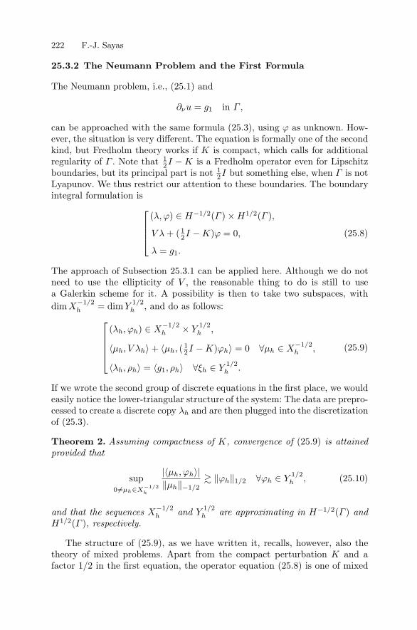
222 F.-J. Sayas
25.3.2 The Neumann Problem and the First Formula
The Neumann problem, i.e., (25.1) and
∂νu = g1 in Γ ,
can be approached with the same formula (25.3), using ϕ as unknown. How-ever, the situation is very different. The equation is formally one of the secondkind, but Fredholm theory works if K is compact, which calls for additionalregularity of Γ . Note that 1
2I −K is a Fredholm operator even for Lipschitzboundaries, but its principal part is not 1
2I but something else, when Γ is notLyapunov. We thus restrict our attention to these boundaries. The boundaryintegral formulation is
⎡⎢⎢⎣
(λ, ϕ) ∈ H−1/2(Γ ) ×H1/2(Γ ),
V λ+ (12I −K)ϕ = 0,
λ = g1.
(25.8)
The approach of Subsection 25.3.1 can be applied here. Although we do notneed to use the ellipticity of V , the reasonable thing to do is still to usea Galerkin scheme for it. A possibility is then to take two subspaces, with
dimX−1/2h = dimY
1/2h , and do as follows:
⎡⎢⎢⎢⎣
(λh, ϕh) ∈ X−1/2h × Y
1/2h ,
〈µh, V λh〉 + 〈µh, (12I −K)ϕh〉 = 0 ∀µh ∈ X
−1/2h ,
〈λh, ρh〉 = 〈g1, ρh〉 ∀ξh ∈ Y1/2h .
(25.9)
If we wrote the second group of discrete equations in the first place, we wouldeasily notice the lower-triangular structure of the system: The data are prepro-cessed to create a discrete copy λh and are then plugged into the discretizationof (25.3).
Theorem 2. Assuming compactness of K, convergence of (25.9) is attainedprovided that
sup0=µh∈X
−1/2h
|〈µh, ϕh〉|‖µh‖−1/2
‖ϕh‖1/2 ∀ϕh ∈ Y1/2h , (25.10)
and that the sequences X−1/2h and Y
1/2h are approximating in H−1/2(Γ ) and
H1/2(Γ ), respectively.
The structure of (25.9), as we have written it, recalls, however, also thetheory of mixed problems. Apart from the compact perturbation K and afactor 1/2 in the first equation, the operator equation (25.8) is one of mixed

25 Direct BEM with Discretization of All Operators 223
type with elliptic diagonal operator. We can then try (25.9) by dropping thecondition of equality of dimensions of the subspaces. Theorem 2 still holds.
For (25.10), it is necessary that dimX−1/2h ≥ dimY
1/2h . The system cannot
be understood anymore as preprocessing the data and substituting, althoughUzawa-type iterations can be applied to avoid working with the full system.These methods can be rewritten as a sequence of preprocesses for the data andsubstitutions, only in reverse order (solving a sequence of Dirichlet problemsinstead of the Neumann one).
25.3.3 Use of the Second Formula
The use of (25.4) as the basic boundary integral equation reverses the roles ofthe unknowns in the considerations above. The Neumann problem is now anelliptic one (W is the associated operator) and works with a simple prepro-cessing of the incoming datum, not needing the hypothesis on compactness ofK. The Dirichlet problem now leads to an equation of the second kind, andeverything works as above, assuming that K is compact.
25.3.4 Mixed Boundary Conditions
A similar approach can easily be applied to the mixed BVP. We will sim-ply sketch how the method works. Assume that Γ is subdivided into twononoverlapping, nontrivial parts ΓD and ΓN , and that we have the boundaryconditions
u = g0 in ΓD, ∂νu = g1 in ΓN ,
for (25.1). We first create any extension of g0 to H1/2(Γ ), say g0. Let H :=ρ ∈ H1/2(Γ ) | ρ ≡ 0, in ΓD. Using (25.3), we can deal with the problemby writing the system
⎡⎢⎢⎢⎢⎢⎣
(λ,ϕ0, ρ) ∈ H−1/2(Γ ) ×H ×H1/2(Γ ),
V λ+ (12I −K)ϕ0 + (1
2I −K)ρ = 0,
〈λ, χ〉 = 〈g1, χ〉 ∀χ ∈ H,
ρ = g0.
Then ϕ = ϕ0+g0 is the full Dirichlet datum and λ is the full Neumann datum.The compactness of K becomes relevant again at the numerical level. We can
use two spaces X−1/2h and Y
1/2h , assuming that dimX
−1/2h = dimY
1/2h , and a
third space Hh := Y1/2h ∩H. The associated Petrov–Galerkin method
⎡⎢⎢⎢⎢⎢⎢⎣
(λh, ϕ0h, ρh) ∈ X
−1/2h ×Hh × Y
1/2h ,
〈µh, V λh〉 + 〈µh, (12I −K)ϕ0
h〉 + 〈µh, (12I −K)ρh〉 = 0 ∀µh ∈ X
−1/2h ,
〈λh, χh〉 = 〈g1, χh〉 ∀χh ∈ Hh,
〈ηh, ρh〉 = 〈ηh, g0〉 ∀ηh ∈ X−1/2h ,

224 F.-J. Sayas
preprocesses the extended Dirichlet datum and then works the whole methodin the sense of Subsection 25.3.2.
Theorem 3. Assuming the compactness of K, approximation properties forall the discrete spaces, and the inf-sup condition
sup0 =ξh∈Hh
|〈λh, χh〉|‖χh‖1/2
‖λh‖−1/2 ∀λh ∈ X−1/2h ,
the above method converges.
25.3.5 Other
Very similar ideas apply very naturally in transmission problems, be theytreated with systems of boundary integral operators or with coupled interior-boundary problems, ready for the application of BEM–FEM coupling tech-niques. Such ideas appear in the background of the analytical and computa-tional tools developed in [RS06], [RS07], and related work.
25.4 Appendix: Petrov–Galerkin Methods
Consider two Hilbert spaces H1 and H2 and a linear variational problem
[u ∈ H1,
a(u, v) = ℓ(v) ∀v ∈ H2,(25.11)
where a : H1 × H2 → R is a continuous bilinear form and ℓ is any elementof the dual of H2. The well posedness of the problem is characterized by theinvertibility of the operator A : H1 → H ′
2
Au := a(u, · ) : H2 → R,
and means that (25.11) is uniquely solvable for any ℓ, and that the solutionoperator is bounded. Let Hh
α ⊂ Hα (α ∈ 1, 2) be two sequences of finite-dimensional spaces, directed on the parameter h → 0, with the restrictiondimHh
1 = dimHh2 . A Petrov–Galerkin method for (25.11), associated with
the spaces Hh1 and Hh
2 , is a scheme of the form
[uh ∈ Hh
1 ,
a(uh, vh) = ℓ(vh) ∀vh ∈ Hh2 .
(25.12)
Equations (25.12) are equivalent to a square linear system with the samedimension as that of the discrete spaces. The concept of stability of the schemeis that of unique solvability of the equations together with a uniform bound(for all h and all u)

25 Direct BEM with Discretization of All Operators 225
‖uh‖ ‖u‖,where the expression ah bh (we will also use the reversed symbol ) meansthat there exists a positive constant C > 0, independent of h and of the quan-tities it multiplies, such that ah ≤ C bh. Stability is equivalent to a uniformBabuska–Brezzi condition
sup0=vh∈Hh
2
|a(uh, vh)|‖vh‖
‖uh‖ ∀uh ∈ Hh1 . (25.13)
Notice that (25.13) already implies unique solvability of the associated sys-tem. Because of the Cea–Polski estimate, convergence (i.e., convergence forarbitrary right-hand sides) is equivalent to stability plus the approximationproperty
infχh∈Hh
1
‖u − χh‖ h→0−→ 0 ∀u ∈ H1. (25.14)
The sequence of spaces Hh1 is said to be approximating in H1 if (25.14) holds.
Sometimes stability is only considered in an asymptotic way, that is, beginningwith h small enough. The sense of this is the fact that the equations could benoninvertible for h large, or that the inherent constant in (25.13) could evolveto a stable regime as h decreases and the values for h large are nonoptimal.
Proposition 1 (Discrete Fredholm property). Convergence is preservedunder compact perturbations of the operator A; namely, if K is compact, A+Kis one-to-one, and the Petrov–Galerkin method with spaces Hh
1 and Hh2 is
convergent for A, then the method is convergent for A + K.
Finally, note that if dimHh1 = dimHh
2 , as we have assumed, then the roleof these spaces in condition (25.13) can be reversed. When the dimensions donot coincide, the condition ceases to be symmetrical. It is then equivalent tothe injectivity of the discrete operator Ah : Hh
1 → (Hh2 )′ defined by
Ahuh := a(uh, · ) : Hh2 → R,
together with the uniform boundedness of its Moore–Penrose pseudoinverse.
References
[BF91] Brezzi, F., Fortin, M.: Mixed and Hybrid Finite Element Methods.Springer, New York (1991).
[GH95] Gatica, G.N., Hsiao, G.C.: Boundary-Field Equation Methods for a Classof Nonlinear Problems. Longman, Harlow (1995).
[K99] Kress, R.: Linear Integral Equations, 2nd ed. Springer, New York (1999).[M00] McLean, W.: Strongly Elliptic Systems and Boundary Integral Equations.
Cambridge University Press, Cambridge (2000).

226 F.-J. Sayas
[RS06] Rapun, M.-L., Sayas, F.-J.: Boundary integral approximation of a heat-diffusion problem in time-harmonic regime. Numer. Algorithms, 41, 127–160 (2006).
[RS07] Rapun, M.-L., Sayas, F.-J.: Boundary element simulation of thermalwaves. Arch. Comput. Methods Engrg, 14, 3–46 (2007).
[S03] Steinbach, O.: Stability Estimates for Hybrid Coupled Domain Decompo-sition Methods. Springer, Berlin (2003).
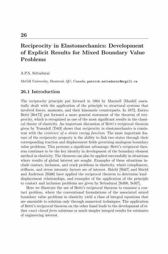
26
Reciprocity in Elastomechanics: Developmentof Explicit Results for Mixed Boundary ValueProblems
A.P.S. Selvadurai
McGill University, Montreal, QC, Canada; [email protected]
26.1 Introduction
The reciprocity principle put forward in 1864 by Maxwell [Max64] essen-tially dealt with the application of the principle to structural systems thatinvolved forces, moments, and their kinematic counterparts. In 1872, EnricoBetti [Bet72] put forward a more general statement of the theorem of reci-procity, which is recognized as one of the most significant results in the classi-cal theory of elasticity. An important discussion of Betti’s reciprocal theoremgiven by Truesdell [Tr63] shows that reciprocity in elastomechanics is consis-tent with the existence of a strain energy function. The most important fea-ture of the reciprocity property is the ability to link two states through theircorresponding traction and displacement fields governing analogous boundaryvalue problems. This presents a significant advantage; Betti’s reciprocal theo-rem continues to be the key identity in development of the boundary elementmethod in elasticity. The theorem can also be applied successfully in situationswhere results of global interest are sought. Examples of these situations in-clude contact, inclusion, and crack problems in elasticity, where compliances,stiffness, and stress intensity factors are of interest. Shield [Sh67] and Shieldand Anderson [Sh66] have applied the reciprocal theorem to determine load–displacement relationships, and examples of the application of the principleto contact and inclusion problems are given by Selvadurai [Sel00, Sel07].
Here we illustrate the use of Betti’s reciprocal theorem to examine a con-tact problem, where the conventional formulations of the associated mixedboundary value problems in elasticity yield a class of integral equations thatare amenable to solution only through numerical techniques. The applicationof Betti’s reciprocal theorem on the other hand leads to the development of ei-ther exact closed form solutions or much simpler integral results for estimatesof engineering interest.

228 A.P.S. Selvadurai
26.2 A Contact Problem for a Half-Space
The problem involving the direct axisymmetric loading of the rigid circularpunch was examined by Boussinesq [Bou85] using the analogy with potentialtheory and later by Harding and Sneddon [Har45], who formulated the mixedboundary value problem as a set of dual integral equations, reducing them to asingle integral equation of the Abel-type, which was solved in an exact fashion.As a special case, we restrict attention to the situation where the contactbetween a rigid circular indentor with a flat smooth base initiated by the loadP is perturbed by a concentrated normal load Q∗ that acts at an exteriorlocation on the surface of the half-space (Figure 26.1(a)). The objective is
(a) (b)
Fig. 26.1. Interaction of a rigid indentor and an externally placed load. (a) Thecontact problem. (b) The reduced mixed boundary value problem.
to determine the additional axial displacement and rotation of the smoothindentor as a result of this external load. Since the classical elasticity problemis linear, we can superimpose the effects of P and Q∗, provided there is noseparation at the smoothly indenting interface. We restrict attention to theanalysis of the interaction between a smoothly interacting rigid indentor with aflat base with a bilateral contact (i.e., capable of sustaining tensile tractions)and the externally placed force Q∗. If the contact is bilateral, the smoothindentor will experience a rigid body translation and a rigid body rotationduring the application of the external load Q∗. We now apply corrective forceresultants in the form of an axial force Q and a moment M , such that thedisplacement of the indentor is suppressed (Figure 26.1(b)). The resultingmixed boundary value problem can be formulated in relation to the half-spaceregion z ≥ 0, as follows:
uz(r, θ, 0) = 0, 0 ≤ θ ≤ 2π, 0 ≤ r ≤ a, (26.1)
σzz(r, θ, 0) = −p(r, θ), 0 ≤ θ ≤ 2π, a < r < ∞, (26.2)
σrz(r, θ, 0) = 0, 0 ≤ θ ≤ 2π, 0 < r < ∞, (26.3)

26 Reciprocity in Elastomechanics 229
where p(r, θ) is an even function of θ.To solve the mixed boundary value problem, we make use of the Han-
kel transformation-based solutions of the equations of elasticity presented byMuki [M60]. It can be shown that when the condition (26.3) pertaining tozero shear tractions is satisfied on z = 0, the displacement uz(r, θ, 0) and thenormal stress σzz(r, θ, 0) can be expressed in the following forms:
[c]uz(r, θ, 0) = 2(1 − ν)
∞∑
m=0
Hm[ξ−2 Ψm(ξ); r] cos mθ,
σzz(r, θ, 0) = −2µ
∞∑
m=0
Hm[ξ−1 Ψm(ξ); r] cos mθ,
where
Hm[Φ(r); ξ] =
∫ ∞
0
r Φ(r) Jm(ξr) dr
is the mth order Hankel operator and Ψm(ξ) are unknown functions to bedetermined by satisfying the mixed boundary conditions (26.1) and (26.2).Assuming that p(r, θ) admits a representation of the form
p(r, θ) = 2µ∞∑
m=0
gm(r) cos mθ,
we see that the mixed boundary conditions (26.1) and (26.2) yield the follow-ing sets of dual integral equations for the unknown functions Ψm(ξ):
Hm[ξ−2 Ψm(ξ); r] = 0, 0 ≤ r ≤ a, (26.4)
Hm[ξ−1 Ψm(ξ); r] = gm(r), a < r < ∞. (26.5)
The solution of the dual systems indicated by (26.4) and (26.5) is given byseveral authors including Noble [N58] and Sneddon and Lowengrub [Sn69], andthe details will not be repeated. It is sufficient to note that for the concentratedexternal loading of the half-space
[g0(r); gm(r)] =Q∗ a δ(r − λa)
8π2 µ r[1; 2],
where δ(r − λa) is the Dirac delta distribution and the contact stress distri-bution at the interface region 0 ≤ r ≤ a is given by
σzz(r, θ, 0) =2Q∗
π2
∞∑
m=0
( r
λa
)m
cosmθ
∫ ∞
a
tH(λa− t) dt√λ2a2 − t2 (t2 − r2)3/2
and H(λa− t) is the Heaviside step function. The explicit expression for σzz
in the contact region of the indentor is given by

230 A.P.S. Selvadurai
σzz(r, θ, 0) =Q∗ √λ2 − 1
a2π2√ρ2 − 1 [λ2 + ρ2 − 2λρ cos θ]
, (26.6)
where ρ = r/a. The result (26.6) can be used to determine the force Q andthe resultant moment M that should be applied to the indentor in order tomaintain the axial displacements zero within the indentor region. It can beshown that
Q =2Q∗
πsin−1
(1
λ
), M = Q∗λa
[1 − 2
π
tan−1
√λ2 − 1 +
√λ2 − 1
λ2
].
It remains now to apply equal and opposite force resultants directly to therigid punch to render the rigid punch free of force resultants. This aspectwill be discussed in detail in the next section, but it is sufficient to note herethat the displacement of the rigid punch in bilateral smooth contact with theelastic half-space region under the action of an external surface load Q∗ isgiven by
uz(r, θ, 0) =Q∗(1 − ν)
4µa
[2
πsin−1
(1
λ
)
+3
2λ ρ cos θ
1 − 2
πtan−1
√λ2 − 1 − 2
π
√λ2 − 1
λ2
], 0 ≤ r ≤ a.
26.3 Solution of the Contact Problem via Betti’sReciprocal Theorem
We now apply Betti’s reciprocal theorem of the solution to the nonclassicalcontact problem shown in Figure 26.2(a). The auxiliary solution required toapply Betti’s theorem relates to the problem of a smoothly indenting circularpunch with a flat base, which is subjected to an eccentric load Q∗ acting ata distance ζa from the center of the indentor (Figure 26.2(b)). The eccentricloading induces a rigid body displacement w0 at the center of the circularpunch and a rotation ϑ0 within the indentor area. If there is no separationwithin the contact region, the displacement boundary conditions associatedwith the eccentric loading are
uz(r, θ, 0) = w0, 0 ≤ r ≤ a, (26.7)
uz(r, θ, 0) = ϑ0r cos θ, 0 ≤ r ≤ a. (26.8)
In addition, the traction boundary conditions applicable to problems are
σzz(r, θ, 0) = 0, 0 ≤ θ ≤ 2π, a < r < ∞, (26.9)
σrz(r, θ, 0) = 0, 0 ≤ θ ≤ 2π, 0 ≤ r < ∞. (26.10)

26 Reciprocity in Elastomechanics 231
(a) (b)
Fig. 26.2. The reciprocal states. (a) The contact problem. (b) The auxiliary solu-tion.
Considering a Hankel transformation development of the governing equations,the conditions (26.7)–(26.10) yield a set of dual integral equations of the forms
H0[ξ−1 A1(ξ); r] = w0, 0 ≤ r ≤ a,
H0[A1(ξ); r] = 0, a < r < ∞,
and
H1[ξ−1 A2(ξ); r] = ϑ0, 0 ≤ r ≤ a,
H1[A2(ξ); r] = 0, a < r < ∞,
where A1(ξ) and A2(ξ) are unknown functions.The solution of these dual systems is standard, and details are given by
Sneddon [Sn75]. The result of interest to the application of the reciprocaltheorem involves the displacements of the indentor and the region exterior tothe indentor due to the eccentric loading; these can be expressed as follows:
uz(r, θ, 0) =Q(1 − ν)
4µa
[1 +
3ζr cos θ
2a
], 0 ≤ r ≤ a, (26.11)
uz(r, θ, 0) =Q(1 − ν)
4µa
[2
πsin−1
(ar
)+
3ζr cos θ
2a
×
1 − 2
πtan−1
(√r2 − a2
a
)− 2a
π
√r2 − a2
r2
], a ≤ r ≤ ∞.
(26.12)
Consider now the following reciprocal states. The first involves the eccentricdisplacement w∗ of the rigid circular indentor at a point within it (ζa, 0, 0), dueto the action of an external normal load Q∗ acting at the location (λa, 0, 0)(Figure 26.2(a)). The value of w∗ can be obtained from (26.11). The sec-ond considers the displacement w at an external point on the surface of the

232 A.P.S. Selvadurai
traction-free half-space (λa, 0, 0) due to the application of an eccentric loadthat acts at a point (ζa, 0, 0) within the indentor region (Figure 26.2(b)). Thevalue of w∗ can be obtained from (26.12). In both cases, the smooth contact isassumed to be bilateral and it is assumed that no separation takes place at thecontact zone. Furthermore, the choice of θ = 0 is simply to illustrate the reci-procity relationship and the result can be generalized to include any arbitrarylocation both within the indentor region and exterior to it. By comparingthese results, we clearly see that
Q∗ w = Q w∗.
We can generalize the result to include the point of application of Q∗ as(λa, φ, 0) and the point within the rigid indentor where the displacement issought by (ρa, 0, 0). The reciprocal relationship gives the result
w0 =Q∗(1 − ν)
4µa
[2
πsin−1
(1
λ
)+
3λρ
2cos (θ − φ)
×(
1 − 2
π
tan−1
√λ2 − 1 +
√λ2 − 1
λ2
)].
26.4 The Cable Jacking Test
The cable jacking test refers to an indentation problem where a test plateresting on the surface of a geologic medium is subjected to loading via aself-stressing system of reaction points located within the medium. The in-terpretation of the test results is made through the results of a Boussinesqindentation problem applicable to the test configuration, void of any influencesof the reaction forces located within the geologic medium. The conventionalmethod of providing a reaction is to consider an axisymmetric load that islocated along the axis of the indenting plate. (See, e.g., Zienkiewicz and Stagg[Z67].) The studies by Selvadurai [Sel78], [Sel79] extended the axisymmetricproblem in the theory of elasticity to explicitly evaluate the influence of thelocation of the internal axisymmetric equilibrating force. The solution for thedisplacement of a smoothly indenting rigid circular plate of radius a that issubjected to an external axial force and an internal axial force located at adistance from the rigid plate and acting in a direction opposite to a is givenby
w0 =P (1 − ν)
4aµ
(1 − PM
P
2
πtan−1
(ac
)+
ac
π(1 − ν)(a2 + c2)
).
The extension of the analysis of the cable jacking test to include other formsof internal load distributions is nonroutine. Consider the test arrangementshown in Figure 26.3, where the reactive loads are provided by concentratedequilibrating forces that are located at the interior of the half-space region.
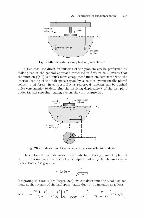
26 Reciprocity in Elastomechanics 233
Fig. 26.3. The cable jacking test in geomechanics.
In this case, the direct formulation of the problem can be performed bymaking use of the general approach presented in Section 26.2, except thatthe function p(r, θ) is a much more complicated function, associated with theinterior loading of the half-space region by a pair of symmetrically placedconcentrated forces. In contrast, Betti’s reciprocal theorem can be appliedquite conveniently to determine the resulting displacement of the test plateunder the self-stressing loading system shown in Figure 26.3.
Fig. 26.4. Indentation of the half-space by a smooth rigid indentor.
The contact stress distribution at the interface of a rigid smooth plate ofradius a resting on the surface of a half-space and subjected to an axisym-metric load P ∗ is given by
σzz(r, 0) =P ∗
πa√a2 − r2
.
Integrating this result (see Figure 26.4), we can determine the axial displace-ment at the interior of the half-space region due to the indentor as follows:
w∗(l, c) =P ∗(1 − ν)
4µa
[1
π2
∫ a
0
[∫ 2π
0
1
φ√a2 − r2
1 +
c2
2(1 − ν)φ2
dθ
]ξdξ
],
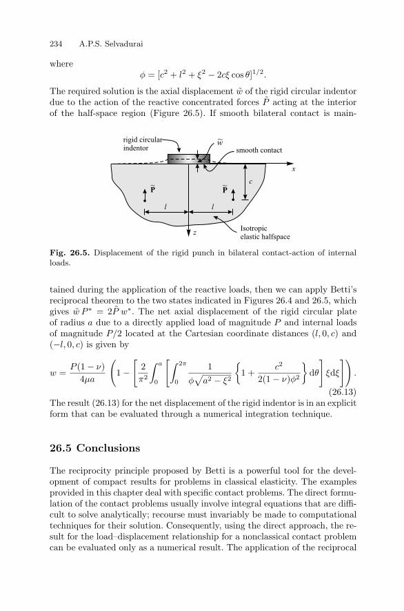
234 A.P.S. Selvadurai
whereφ = [c2 + l2 + ξ2 − 2cξ cos θ]1/2.
The required solution is the axial displacement w of the rigid circular indentordue to the action of the reactive concentrated forces P acting at the interiorof the half-space region (Figure 26.5). If smooth bilateral contact is main-
Fig. 26.5. Displacement of the rigid punch in bilateral contact-action of internalloads.
tained during the application of the reactive loads, then we can apply Betti’sreciprocal theorem to the two states indicated in Figures 26.4 and 26.5, whichgives w P ∗ = 2P w∗. The net axial displacement of the rigid circular plateof radius a due to a directly applied load of magnitude P and internal loadsof magnitude P/2 located at the Cartesian coordinate distances (l, 0, c) and(−l, 0, c) is given by
w =P (1 − ν)
4µa
(1 −
[2
π2
∫ a
0
[∫ 2π
0
1
φ√a2 − ξ2
1 +
c2
2(1 − ν)φ2
dθ
]ξdξ
]).
(26.13)The result (26.13) for the net displacement of the rigid indentor is in an explicitform that can be evaluated through a numerical integration technique.
26.5 Conclusions
The reciprocity principle proposed by Betti is a powerful tool for the devel-opment of compact results for problems in classical elasticity. The examplesprovided in this chapter deal with specific contact problems. The direct formu-lation of the contact problems usually involve integral equations that are diffi-cult to solve analytically; recourse must invariably be made to computationaltechniques for their solution. Consequently, using the direct approach, the re-sult for the load–displacement relationship for a nonclassical contact problemcan be evaluated only as a numerical result. The application of the reciprocal

26 Reciprocity in Elastomechanics 235
theorem, however, enables the development of the load-displacement resultin either a compact integral form or in an exact closed form. In the aboveexamples, where the external load is located at the surface of the half-space,the systems of dual integral equations governing the problem involving thedirect formulation can be solved in a convenient way. If the external load-ing is located at an arbitrary point within the half-space region, the solutionis not as straightforward and can be developed only through the numericaltechnique that converts the dual integral equations to either an Abel-typeor a Fredholm-type integral equation of the second kind. The application ofthe reciprocal theorem is a more convenient way of developing solutions tothe external load-rigid indentor interaction problem. The main reason for theease of application of Betti’s reciprocal theorem stems from the fact that theauxiliary solutions associated with these problems can be obtained in compactforms through the solution of a set of dual integral equations. The method-ologies described in this chapter can be extended to include other classes ofreciprocal relationships associated with inhomogeneous media, elastodynamicproblems, and poroelasticity problems.
Acknowledgement. This work was supported through the 2003 Max Planck For-schungspreis in the Engineering Sciences awarded by the Max Planck Gesellschaft,Germany.
References
[Bet72] Betti, E.: Teoria dell’Elasticita, Nuovo Cimento Ser. II, VII, VIII (1872).[Bou85] Boussinesq, J.: Application des Potentiels a l’Etude de l’Equilibre et du
Mouvement des Solides. Gauthier-Villars, Paris (1885).[Har45] Harding, J.W., Sneddon, I.N.: The elastic stresses produced by the inden-
tation of the plane surface of a semi-infinite solid by a rigid punch. Camb.Phil. Soc., 41, 16–26 (1945).
[M60] Muki, R.: Asymmetric problems in the theory of elasticity for a semi-infinite solid and a thick plate. In: Sneddon, I.N., Hill, R. (eds.), Progressin Solid Mechanics, vol. 1. North-Holland, Amsterdam (1960), pp. 339–349.
[Max64] Maxwell, J.C.: On the calculation of equilibrium and stiffness of frames.Phil. Mag., 27, 294–299 (1864).
[N58] Noble, B.: Certain dual integral equations. J. Math. Phys., 37, 128–136(1958).
[Sel78] Selvadurai, A.P.S.: The interaction between a rigid circular punch on anelastic halfspace and a Mindlin force. Mech. Res. Comm., 5, 57–64 (1978).
[Sel79] Selvadurai, A.P.S.: The displacement of a rigid circular foundation an-chored to an isotropic elastic halfspace. Geotechnique, 29, 195–202 (1979).
[Sel00] Selvadurai, A.P.S.: On the mathematical modelling of certain fundamentalelastostatic contact problems in geomechanics. In: Zaman, M., Gioda, G.,Booker, J.R. (eds.), Modelling in Geomechanics. Wiley, New York (2000).

236 A.P.S. Selvadurai
[Sel07] Selvadurai, A.P.S.: The analytical method in geomechanics. Appl. Mech.Reviews, 60, 87–106 (2007).
[Sh66] Shield, R.T., Anderson, C.A.: Some least work principles for elastic bodies.Z. Angew. Math. Phys., 17, 663–676 (1966).
[Sh67] Shield, R.T.: Load–displacement relations for elastic bodies. Z. Angew.Math. Phys., 18, 682–693 (1967).
[Sn69] Sneddon, I.N., Lowengrub, M.: Crack Problems in the Classical Theory ofElasticity. Wiley, New York (1969).
[Sn75] Sneddon, I.N.: Application of Integral Transforms in the Theory of Elas-ticity. Springer, Wien (1975).
[Tr63] Truesdell, C.: The meaning of Betti’s reciprocal theorem. J. Research Nat.Bur. Standards, 67B, 85–86 (1963).
[Z67] Zienkiewicz, O.C., Stagg, K.G.: Cable method of in-situ rock testing. Int.J. Rock Mech. Min. Sci., 4, 273–300 (1967).

27
Integral Equation Modeling of ElectrostaticInteractions in Atomic Force Microscopy
Y. Shen, D.M. Barnett, and P.M. Pinsky
Stanford University, CA, USA; [email protected], [email protected],[email protected]
27.1 Introduction
Since its invention in 1986 [BQG86], the atomic force microscope (AFM) hasevolved as a major tool for characterizing materials. Of the several operationalmodes of the AFM, the noncontact mode is normally used to determine thesample surface charge distribution. In this range of tip–sample separation,the Coulombic interaction between the tip and the sample dominates overmagnetic and van der Waal forces. Despite the simple and explicit expressionof Coulomb’s law, mapping AFM images to sample charge distributions cannotbe done in a straightforward way because of the finite size of the AFM tipand the roughness of the sample. Thus, researchers have been approachingthis inverse problem from the opposite direction by making efforts to predictAFM measurements based on assumed sample properties. Numerous modelshave been proposed to tackle this electrostatic problem.
For the case in which both the tip and the sample are conductors, someprevious approaches treat the surfaces of these two objects as two equipoten-tials due to an assumed distribution of source and image charges relative to thesample surface, for example, a single charge [HXOS95], a series of point charges[BGL97], or a uniformly charged line [HBS91]. Another approach replaces thetip with a geometrical object and either solves the Laplace equation in aclosed form (e.g., the spherical-tip model [TSRM89] and the hyperboloidal-tip model [PSPCM94]) or approximates the electric field lines using circulararcs and straight lines (e.g., the models that treat the tip as a cone with aspherical apex [HJGB98] or a parabolic apex [CGB01]). In all of these models,a geometrical approximation error of the tip is introduced.
On the other hand, numerical schemes have also been developed to com-pute the tip–sample interaction in which the tip shape information is fullytaken into account (up to the mesh error). Belaidi et al. [BLGLP98] proposeda finite element setup for this external Dirichlet problem in which the infi-nite domain (the vacuum outside the tip and the sample) was truncated toa finitely large cylindrical domain, but this truncated domain still required

238 Y. Shen, D.M. Barnett, and P.M. Pinsky
a three-dimensional mesh. In contrast, Strassburg et al. [SBR05] employed aboundary element method to reconstruct the images of a conductive samplein which only the tip surface had to be meshed, while the sample surface withvanishing boundary value was accommodated by an image term in the Green’sfunction. However, in [SBR05], the sample is restricted to be conductive.
Independently, we have developed a boundary integral equation approachsimilar to that of [SBR05], but our formulation applies not only to conductivesamples but also to dielectric ones, with arbitrary distributions of surfaceand/or volumetric charges that can be taken into account; thus, our work isapplicable to a wider range of problems.
27.2 Conductive Sample
27.2.1 Boundary Value Problem
In our model, only the Coulombic interaction between the AFM tip and thesample is taken into account, whereas both the van der Waal and the magneticinteractions are ignored, resulting in a classical electrostatic problem. Becausethe AFM cantilever only contributes a constant shift to the tip–sample inter-action (see, e.g., [CGB01]), and the interpretation of AFM images primarilyrelies only on the contrast between regions rather than on the actual magni-tudes of interactions, it seems reasonable that the cantilever not be includedin our model. Furthermore, the tip is truncated to have a height of 100 nm,assuming that such a height is enough to capture the variation in tip–sampleinteraction relative to a homogeneous sample, as the tip scans the samplewhile maintaining a constant separation.
The AFM tip is almost always manufactured to be conductive, whereasthe sample may be either conductive or dielectric. If the sample is also con-ductive, the electrostatic problem becomes an exterior Dirichlet problem witha single homogeneous domain Ω (the vacuum or air between the tip and thesample), over which Laplace’s equation (∇2φ = 0) holds, as shown in Figure27.1. Dirichlet boundary conditions are imposed on both the tip surface Stip
(φ = φ0) and the sample surface Ssam(φ = 0). For simplicity, throughout thischapter, the sample is assumed to be flat and semi-infinite.
27.2.2 Boundary Integral Equation
Classical potential theory (see, e.g., [JS77]) yields the boundary integral equa-tion
∫
Stip
G(#r; #r′)σ(#r)dS(#r) = φ0, ∀#r′ ∈ Stip, (27.1)
where

27 Integral Equation Modeling of Electrostatic Interactions in AFM 239
Fig. 27.1. Schematic of the exterior Dirichlet problem that describes the electro-static interaction between an AFM tip and a conductive sample.
G(#r; #r′) := Φ(#r − #r′) − Φ(#r − #r′im),
which is the Green’s function that vanishes at the sample surface, Φ(#r− #r′) :=
(4πǫ0|#r − #r′|)−1 being the fundamental solution to the Laplace equation in
free space (ǫ0 = 8.854× 10⁻¹² F/m is the permittivity of vacuum). #r′im is the
image position of the source point #r′ with respect to the sample plane; and
σ(#r) := ǫ0∂φ(#r)
∂#nr,
which is the unknown charge density on the tip surface; #nr is the unit outwardnormal of Ω, thus pointing inward on the tip.
27.2.3 Numerical Analysis and Postprocessing
Equation (27.1) is a Fredholm boundary integral equation of the first kind, theunknown of which is the moment of a single-layer potential. The boundary ele-ment method was employed to solve it. First, the tip surface was meshed intoeither four-node quadrilaterals or eight-node serendipity elements [Beer01,Chapter 3], and the associated interpolation functions were used to representthe unknown surface charge density σ(#r) on the tip. Then, the point collo-cation approach was used to deduce the matrix equation, the unknowns ofwhich are all the nodal σ values. Thereafter, a biconjugate gradient solverwas employed to solve for these unknowns. We adopted the boundary elementcode given in [Beer01] for the assembly and equation-solving processes.
Upon obtaining σ(#r), the tip–sample capacitance C is, by definition, readyto compute as
C =1
φ0
∫
Stip
σ(#r)dS(#r).
To calculate the net tip–sample force #f , we integrate the traction associ-ated with the Maxwell stress over the tip surface as

240 Y. Shen, D.M. Barnett, and P.M. Pinsky
fi = −∫
Stip
σ(#r)2
2ǫ0nridS(#r), (27.2)
where i = 1, 2, 3, denoting the axial directions in the Cartesian coordinateframe, of which x3 is chosen so as to parallel the tip axis and to point outwardfrom the flat sample.
To compute the force gradient component ∂fi/∂xtipj , where #xtip denotes
the tip apex position, we take the derivative of (27.2) with respect to xtipj and
have∂fi
∂xtipj
= −∫
Stip
σ(#r)
ǫ0
∂σ(#r)
∂xtipj
nidS(#r), (27.3)
where ∂σ(#r)/∂xtipj can be computed by taking the derivative of (27.1) with
respect to xtipj and rearranging the terms to have
∫
Stip
G(#r; #r′)∂σ(#r)
∂xtipj
dS(#r) = −∫
Stip
∂G(#r; #r′)
∂xtipj
σ(#r)dS(#r), ∀#r′ ∈ Stip. (27.4)
The matrix equation associated with (27.4) has the same coefficient matrix asthat for (27.1) since they have the same integral operator on the unknowns.
27.2.4 Convergence Study
To verify the numerical scheme proposed above, a benchmark problem withan exact analytical solution is useful. We chose the sphere–plane capacitancesystem, and looked up and completed the solution by [Smythe68, Chapter V].The complete solution is also provided in the Appendix.
We applied the boundary element method to a sphere–plane capacitanceproblem corresponding to a typical experimental setup: a sphere with a radiusof 20 nm and a sphere-plane separation of 5 nm. The potential differencebetween the sphere and the plane is set to 1 V.
The absolute errors for the different mesh types and mesh sizes in terms ofnodal σ values, capacitance, force, and force gradient are listed in Table 27.1.The exact solutions for those global quantities are provided in the last row ofTable 27.1. Thus, the relative errors can be obtained by dividing the absoluteerrors by the corresponding exact solutions. The average number of iterationswas obtained by averaging the number of iterations in solving the matrixequations associated with (27.1) and (27.4) using the biconjugate gradientsolver. The convergence criterion was that the elemental relative differencebetween two successive steps is less than 10−4. If the resolution of the force is1 pN, we can deduce the critical mesh parameters to be 2 nm for four-nodequadrilaterals and 8 nm for eight-node serendipity elements. The serendipityelement is favored for less cost in assembly time and better approximation tothe curved tip surface.

27 Integral Equation Modeling of Electrostatic Interactions in AFM 241
Subsequent results for the tip-sample interaction are, accordingly, basedon the 8 nm serendipity element.
Table 27.1. Convergence study of the sphere–plane capacitance system.
Mesh type A B C D E F G H
10 76 10 5×10⁻¹ 1×10² 5 1 28 108 9.5 3×10⁻¹ 8×10 4 6×10⁻¹ 2
Four-node 6 165 11.5 2×10⁻¹ 5×10 2 1×10⁻¹ 1quadrilateral 4 370 10 1×10⁻¹ 2×10 1 9×10⁻² 5×10⁻¹
2 1406 12 3×10⁻² 6 3×10⁻¹ 1×10⁻² 1×10⁻¹
1 5480 13.5 7×10⁻³ 2 8×10⁻² 2×10⁻³ 3×10⁻²
20 44 11 1 9×10 7 1 3Eight-node 10 86 11.5 3×10⁻¹ 2×10 1 8×10⁻¹ 6×10⁻¹
serendipity 8 323 14.5 5×10⁻² 2 5×10⁻² 2×10⁻² 5×10⁻²
6 485 10 7×10⁻² 8×10⁻¹ 3×10⁻³ 1×10⁻² 2×10⁻²
4 1124 12.5 5×10⁻² 1×10⁻¹ 8×10⁻³ 1×10⁻³ 3×10⁻³
2 4136 16.5 4×10⁻² 4×10⁻² 6×10⁻³ 3×10⁻⁴ 1×10⁻³
Exact – – – – 3957.47 −84.683 0 46.080solutions
The designation of the columns in Table 27.1 is as follows:
A: Mesh size (nm).B: Number of degrees of freedom.C: Average number of iterations.D: Nodal L2-error (10−3 C/m2).E: Error in C (10−21 F).F: Error in f3 (pN).G: Error in f12 (pN).
H: Error in ∂f3/∂xtip3 (pN/nm).
27.3 Dielectric Sample with Arbitrary Surface and/orVolumetric Charges
27.3.1 Formulation
A dielectric sample is generally no longer an equipotential. It may also havedistributions of surface charge s(#r) and volumetric charge ρ(#r). The partialdifferential equations that govern the problem are Laplace’s equation in theair Ω and Poisson’s equation in the interior of the sample Ωsam, namely:
∇2φ(#r) =
0, if #r ∈ Ω,
−ρ(#r)/K, if #r ∈ Ωsam,

242 Y. Shen, D.M. Barnett, and P.M. Pinsky
where K denotes the sample’s dielectric constant.The continuity equation for the sample surface is
∂φ
∂#n(#r)
∣∣∣∣Ω
− K∂φ
∂#n(#r)
∣∣∣∣Ωsam
= s(#r) ∀#r ∈ Ssam,
where #n points inward of the sample.Now, the counterpart of the boundary integral equation (27.1) is∫
Stip
G(#r; #r′)σ(#r)dS(#r) = φ0 −2
1 + K
∫
Ssam
Φ(#r − #r′)s(#r)dS(#r)
− 2
1 + K
∫
Ωsam
Φ(#r − #r′)ρ(#r)dV (#r), ∀#r′ ∈ Stip,
(27.5)
where
G(#r; #r′) := Φ(#r − #r′) − K − 1
K + 1Φ(#r − #r′im) ∀#r, #r′ ∈ Ω,
which is the Green’s function for the dielectric sample.
27.3.2 Predicted Images for a Test Case
If both s(#r) and ρ(#r) are known, (27.5) can also be solved using the boundaryelement method, as in the case for a conductive sample. Furthermore, thetip-sample forces and their gradients can be obtained via (27.2) and (27.3),respectively.
Thus, using this framework, we can predict AFM images as the tip scansa sample with a constant separation. To exemplify this capability, we usezirconia as a model sample material with a dielectric constant K = 40. Thissample is assumed to have no volumetric charge (ρ(#r) = 0), but only a surfacecharge of density
s(#r) = s(x, y) =s0
3
cos
[k
(x − y√
3
)]+ cos
2ky√3
+ cos
[k
(x +
y√3
)],
where 2π/k = 20 nm, the periodicity of the surface charge and s0 = 17.49e/nm2, corresponding to the maximum surface charge density of a (111) oxy-gen lattice plane of zirconia. Such a surface charge may be due to surfacesegregation of ions. A contour plot of s(#r) is presented in Figure 27.2. TheAFM tip is assumed to be a cone (with a total cone angle of 30) with aspherical apex (with a radius of 20 nm). The height of the cone is truncatedto be 100 nm. Here we use sizes of serendipity elements finer than 8 nm tobetter resolve the sample spatial charge variation (2 nm for the apex and 6nm for the rest of the tip). In the case of zero DC bias between the tip and thesample, predicted images in terms of force and force gradient at the separationof 5 nm are plotted in Figures 27.3 and 27.4, respectively. If the resolution ofthe force difference as the tip scans the sample is 1 pN, we can conclude thatsuch variation in surface charge can be detected by the AFM.

27 Integral Equation Modeling of Electrostatic Interactions in AFM 243
Fig. 27.2. Assumed sample surface charge density relative to s0.
Fig. 27.3. Predicted image in terms of force component f3 (in pN).
Fig. 27.4. Predicted image in terms of force gradient component ∂f3/∂xtip3 (in
pN/nm).
27.4 Conclusions
A unified formulation for the AFM tip–sample electrostatic interaction hasbeen developed in terms of boundary integral equations. To the authors’knowledge, these are the first such computations for dielectric samples withcharge distributions. The sample in this chapter is restricted to be semi-infinite

244 Y. Shen, D.M. Barnett, and P.M. Pinsky
and with a flat surface; however, the extension to a finite-sized, nonflat sampleis not difficult to achieve.
With the Maxwell stress tensor, the AFM image due to electrostatic in-teraction can be predicted based on the knowledge of the sample and theexperimental condition.
Acknowledgement. This work has been funded by the Global Climate & EnergyProject, Grant No. 33453.
Appendix: Exact Solution for the Sphere–PlaneCapacitance System
In the sphere–plane capacitance system, we assume that the plane (and thusalso the semi-infinite conductor) is grounded and that the sphere of radius ais at potential φ0. The distance between the sphere center and the plane isdenoted by d.
According to Smythe [Smythe68], the electric field between the sphere andthe plane can be represented by two sets of image charges, one set of whichlocated inside the spherical conductor and the other set inside the semi-infiniteconductor.
If we establish a Cartesian coordinate frame so that the origin coincideswith the sphere center and the z-axis is normal to the plane, then the equationof the plane is given by z = −d, without loss of generality.
Smythe’s two sets of image charges are qn at (0, 0,−sn) and −qnat (0, 0,−2d + sn), n = 1, 2, 3, ..., where
qn := 4πǫ0φ0a sinhαcschnα, sn := a sinh(n− 1)αcschnα,
and α := cosh−1(d/a).Thus, the axisymmetric potential outside the two conductors, φ(ρ, z),
where ρ := (x2 + y2)1/2, is given by
φ(ρ, z) =1
4πǫ0
∞∑
n=1
qn
[ρ2 + (z + sn)2]1/2− qn
[ρ2 + (z + 2d− sn)2]1/2
.
And the surface charge density on the sphere follows as
σ(ρ, z) = ǫ0 sinhα
∞∑
n=1
cschnα
a2 + zsn
[a2 + 2zsn + s2n]3/2
− a2 + 2zd− zsn
[a2 + 2z(2d− sn) + (2d− sn)2]3/2
.
The capacitance can be obtained by summing one set of the charges as

27 Integral Equation Modeling of Electrostatic Interactions in AFM 245
C =1
φ0
∞∑
n=1
qn = 4πǫ0a sinhα
∞∑
n=1
cschnα.
The force component fz and force gradient component ∂fz/∂d can beevaluated by taking the first and second derivatives of the capacitance withrespect to d, respectively, as
fz = −1
2φ2
0
∂C
∂d= 2πǫ0φ
20
∞∑
n=1
cschnα(cothα− n cothnα)
and
∂fz
∂d=
2πǫ0φ20 sinhα
a
×∞∑
n=1
cschnαn2csch 2nα− csch 2α+ n cothnα(n cothnα− cothα)
.
References
[Beer01] Beer, G.: Programming the Boundary Element Method: An Introduc-tion for Engineers. Wiley, New York (2001).
[BGL97] Belaidi, S., Girard, P., Leveque, G.: Electrostatic forces acting on thetip in atomic force microscopy: modelization and comparison with an-alytic expressions. J. Appl. Phys., 81, 1023–1030 (1997).
[BLGLP98] Belaidi, S., Lebon, E., Girard, P., Leveque, G., Pagano, S.: Finite el-ement simulations of the resolution in electrostatic force microscopy.Appl. Phys. A, 66, S239–S243 (1998).
[BQG86] Binnig, G., Quate, C.F., Gerber, Ch.: Atomic force microscope. Phys.Rev. Lett., 56, 930–933 (1986).
[CGB01] Colchero, J., Gil, A., Baro, A.M.: Resolution enhancement and im-proved data interpretation in electrostatic force microscopy. Phys. Rev.B, 64, 245403 (2001).
[HBS91] Hao, H.W., Baro, A.M., Saenz, J.J.: Electrostatic and contact forcesin force microscopy. J. Vac. Sci. Tech. B, 9, 1323–1328 (1991).
[HJGB98] Hudlet, S., Saint Jean, M., Guthmann, C., Berger, J.: Evaluation ofthe capacitive force between an atomic force microscopy tip and ametallic surface. Eur. Phys. J. B, 2, 5–10 (1998).
[HXOS95] Hu, J., Xiao, X.-D., Ogletree, D.F., Salmeron, M.: Imaging the conden-sation and evaporation of molecularly thin films of water with nanome-ter resolution. Science, 268, 267–269 (1995).
[JS77] Jaswon, M.A., Symm, G.T.: Integral Equation Methods in PotentialTheory and Elastostatics. Academic Press, London-New York (1977).
[PSPCM94] Pan, L.H., Sullivan, T.E., Peridier, V.J., Cutler, P.H., Miskovsky,N.M.: Three-dimensional electrostatic potential, and potential-energybarrier, near a tip–base junction. Appl. Phys. Lett., 65, 2151–2153(1994).

246 Y. Shen, D.M. Barnett, and P.M. Pinsky
[SBR05] Strassburg, E., Boag, A., Rosenwaks, Y.: Reconstruction of electro-static force microscopy images. Rev. Scientif. Instrum., 76, 083705(2005).
[Smythe68] Smythe, W.R.: Static and Dynamic Electricity, 3rd ed. McGraw-Hill,New York (1968).
[TSRM89] Terris, B.D., Stern J.E., Rugar, D., Mamin, H.J.: Contact electrifica-tion using force microscopy. Phys. Rev. Lett., 63, 2669–2672 (1989).

28
Integral Representation for the Solution of aCrack Problem Under Stretching Pressure inPlane Asymmetric Elasticity
E. Shmoylova1, S. Potapenko2, and L. Rothenburg2
1 Tufts University, Medford, MA, USA; [email protected] University of Waterloo, ON, Canada; [email protected],[email protected]
28.1 Introduction
The theory of micropolar elasticity (also known as Cosserat or asymmetrictheory of elasticity) was introduced by Eringen [Er66], to eliminate discrepan-cies between the classical theory of elasticity and experiments in cases wheneffects of material microstructure were known to contribute significantly to thebody’s overall deformation, for example, materials with granular microstruc-ture such as polymers or human bones (see Lakes [Lak95], [Lak82], Lakes etal. [LNB90], and Nakamura and Lakes [NL88]). These cases are becoming in-creasingly important in the design and manufacture of modern-day advancedmaterials as small-scale effects become very important in the prediction of theoverall mechanical behavior of these materials.
Several studies relating to investigations of stress distributions around acrack have been undertaken under assumptions of a simplified theory of planeCosserat elasticity by Muhlhaus and Pasternak [MP02], Atkinson and Lep-pington [AtL02], experimentally by Lakes et al. [LNB90], and using the finiteelement method (see Nakamura and Lakes [NL88]).
Recently, Chudinovich and Constanda [CC00] used the boundary integralequation method in a weak (Sobolev) space setting to obtain the solution forfundamental boundary value problems in a theory of bending of classical elas-tic plates. This approach has wide practical applicability because it also coversdomains with reduced boundary smoothness. In addition, it provides an an-swer to the fundamental question of existence and uniqueness of the solution,and gives an opportunity to employ an effective numerical procedure for con-structing a numerical solution, which can be very useful for practical purposes.Furthermore, Chudinovich and Constanda [CC00] extended their method toaccommodate several problems relating to the investigation of stress concen-trations around a crack in classical plates.

248 E. Shmoylova, S. Potapenko, and L. Rothenburg
In several very recent works by Shmoylova et al. (see [SPR06], [SPRa], and[SPRb]), the authors performed a rigorous analysis of interior and exteriorDirichlet and Neumann boundary value problems in plane Cosserat elasticityand obtained the solution to the crack problem arising in this theory in theform of modified integral potentials with unknown distributional densities.Unfortunately, it is very difficult, if not impossible, to find these densitiesanalytically. In this work we apply the boundary element method to obtain anumerical approximation of the solution. This method has been developed byBrebbia [Br78] and has become very popular among researchers in differentareas, including fracture mechanics (see, for example, [AlB93] for referenceson applications of the boundary element method in science and engineering).
In this chapter, we use the boundary element method to find the solutionfor an infinite domain weakened by a crack in plane Cosserat elasticity, whenstresses and couple stresses are prescribed along both sides of the crack (Neu-mann boundary value problem). To illustrate the effectiveness of the methodfor applications, we consider a crack in a human bone that is modeled underassumptions of plane micropolar elasticity. We find the numerical solution forthe stresses around the crack and show that the solution may be reduced tothe classical one if we set all micropolar elastic constants equal to zero. Wecome to the conclusion that there could be up to a 26% difference in the quan-titative characteristics of the stress around a crack in the micropolar case bycomparison with the model when microstructure is ignored (the classical case;see, for example, [Sn69]).
28.2 Preliminaries
In what follows Greek and Latin indices take the values 1, 2 and 1, 2, 3,respectively, the convention of summation over repeated indices is understood,Mm×n is the space of (m×n)-matrices, and a superscript T indicates matrixtransposition.
Let S be a domain in R2 occupied by a homogeneous and isotropic, linearly
elastic micropolar material with elastic constants λ, µ, α, γ, and ε. We use thenotation ‖ · ‖0;S and 〈·, ·〉0;S for the norm and inner product in L2(S)∩Mm×1
for any m ∈ N. When S = R2, we write ‖ · ‖0 and 〈·, ·〉0 .
The state of plane micropolar strain is characterized by a displacementfield u (x′) = (u1 (x′) , u2 (x′) , u3 (x′))T and a microrotation field φ (x′) =(φ1 (x′) , φ2 (x′) , φ3 (x′))T of the form
uα (x′) = uα (x) , u3(x′) = 0,
φα (x′) = 0, φ3(x′) = φ3 (x) ,
where x′ = (x1, x2, x3) and x = (x1, x2) are generic points in R3 and R
2,respectively.
The internal energy density is given by [Sch96]

28 Crack in Plane Asymmetric Elasticity 249
2E (u, v) = 2E0 (u, v) + µ(u1,2 + u2,1)(v1,2 + v2,1)+α(u1,2 − u2,1 + 2u3)(v1,2 − v2,1 + 2v3)+(γ + ε)(u3,1v3,1 + u3,2v3,2),
2E0 (u, v) = (λ + 2µ) (u1,1v1,1 + u2,2v2,2) + λ(u1,1v2,2 + u2,2v1,1).
In what follows we assume that
λ + µ > 0, µ > 0, γ + ε > 0, α > 0.
Clearly, E(u, u) is a positive quadratic form.We consider the boundary stress operator T (∂x) = T (∂/∂xα) defined by
T (ξ) = T (ξα)
=
⎛⎝
(λ + 2µ) ξ1n1 + (µ + α) ξ2n2 (µ − α)ξ1n2 + λξ2n1 2αn2
(µ − α)ξ2n1 + λξ1n2 (λ + 2µ) ξ2n2 + (µ + α) ξ1n1 −2αn1
0 0 (γ + ε)ξαnα
⎞⎠ ,
where n = (n1, n2)T is the unit outward normal to ∂S.
The space of rigid displacements and microrotations F is spanned by thevectors z(1) = (1, 0, 0)T , z(2) = (0, 1, 0)T , and z(3) = (−x2, x1, 1)T .
We consider the matrix of fundamental solutions D(x, y) and the matrixof singular solutions P (x, y) = (T (∂y)D(y, x))T .
We consider an infinite domain with a crack modeled by an open arc Γ0
and assume that Γ0 is a part of a simple closed C2-curve Γ that divides R2
into interior and exterior domains Ω+ and Ω−. In what follows, we denoteby the superscripts + and − the limiting values of functions as x → Γ fromwithin Ω+ or Ω−. Furthermore, we define Ω = R
2\Γ0 and Γ1 = Γ\Γ0. Weintroduce the restriction operators π± to Ω± and the trace operators γ±
0 onΓ0 and γ±
1 on Γ1 from within Ω±, respectively. Let H1,ω(Ω) be the space of allu = u+, u− such that u+ ∈ H1(Ω
+), u− ∈ H1,ω(Ω−), and γ+1 u+ = γ−
1 u−.The space H1(Ω
+) is a standard Sobolev space and H1,ω(Ω−) is a weightedSobolev space defined in [21].
Next, we introduce the corresponding single-layer and double-layer poten-tials, respectively, by
(V ϕ)(x) =
∫
Γ0
D(x, y)ϕ(y) ds(y),
(Wϕ)(x) =
∫
Γ0
P (x, y)ϕ(y) ds(y),
where ϕ ∈ M3×1 is an unknown density matrix.
28.3 Boundary Value Problem
Let us consider the Neumann boundary value problem with the boundaryconditions

250 E. Shmoylova, S. Potapenko, and L. Rothenburg
(Tu)+(x) = g+(x), (Tu)−(x) = g−(x), x ∈ Γ0,
where g+ and g− are prescribed on Γ0. We write δg for the jump of thesequantities across the crack.
The variational formulation of the boundary value problem is as follows.We seek u ∈ H1,ω(Ω) such that
b(u, v) =⟨δg, γ+
0 v+
⟩0;Γ0
+⟨g−, δv
⟩0;Γ0
∀v ∈ H1,ω(Ω), (28.1)
where b(u, v) = 2∫
Ω− E(u−, v−) dx+ 2∫
Ω+ E(u+, v+) dx. Note that (28.1) issolvable only if
〈z, δg〉0;Γ0= 0 ∀z ∈ F .
We define the modified single-layer potential V of density ϕ by
(Vϕ)(x) = (V ϕ)(x) −⟨(V ϕ)0, z
(i)⟩
0;Γ0
z(i)(x), x ∈ R2,
where V ϕ is the single-layer potential, V0 is the boundary operator definedby (V ϕ)0 = γ±
0 π±V ϕ, and z(i)3
i=1 is an L2(Γ0)-orthonormal basis for F .Also, we introduce the modified double-layer potential W of density ψ
(Wψ)(x) = (Wψ)(x) −⟨π0W
+ψ, z(i)⟩
0;Γ0
z(i)(x), x ∈ Ω,
where π0 is the operator of restriction to Γ0.The solution of problem (28.1) may be represented in the form
u = (Vϕ)Ω + Wψ + z, (28.2)
where ϕ and ψ are unknown densities and z ∈ F is arbitrary. The detailedprocedure for obtaining solution (28.2) has been developed by Shmoylova etal. in [SPRb].
28.4 Boundary Element Method
Consider problem (28.1). As shown in [SPRb], the solution to this problemmay be represented in the form (28.2), and the corresponding boundary inte-gral equations are uniquely solvable with respect to distributional densities ϕand ψ. As stated above, these densities cannot be found analytically. To ap-proximate them numerically, we use the boundary element method [GKW03],which makes use of the following classical result.
Lemma 1. (Somigliana formula If u ∈ H1,ω(Ω) is a solution of (28.1) in Ω,then∫
Γ0
[D(x, y)δ (T (∂y)u(y)) − P (x, y)δu(y)] ds(y) =1
2δu(x), x ∈ Γ0, (28.3)
where δ (·) denotes the jump of (·) across the crack.

28 Crack in Plane Asymmetric Elasticity 251
It has been shown in [SPRb] that the density of the modified single-layerpotential may be found in the form ϕ = δ (T (∂y)u(y)) = δg. Now we need tofind the density of the modified double-layer potential ψ = −δu. To achieve
this goal, we divide Γ0 into n elements Γ(k)0 , each of which possesses one node
ξ(k) located in the middle of the element. The values of δg and δu are constantthroughout the element and correspond to the value at the node δg(ξ(k)) andδu(ξ(k)). Then (28.3) becomes
n∑
k=1
∫
Γ(k)0
[D(x, y)δg(ξ(k)) − P (x, y)δu(ξ(k))
]ds(y) =
1
2δu(x), x ∈ Γ0.
Placing x sequentially at all nodes, we obtain the linear algebraic system ofequations
n∑
k=1
(∫
Γ(k)0
D(ξ(i), y) ds(y)
)δg(ξ(k)) −
n∑
k=1
(∫
Γ(k)0
P (ξ(i), y) ds(y)
)δu(ξ(k))
(28.4)
=1
2δu(ξ(i)), i, k = 1, n
with respect to δu(ξi).We note that
∫Γ
(k)0
D(ξ(i), y) ds(y) are defined for any i and k, as in [Sch96].
Solving (28.4), we construct an approximation to ψ. If we introduce theshape function Φk(x) by
Φk(x) =
1, x ∈ Γ
(k)0 ,
0, x ∈ Γ0\Γ (k)0 ,
then the approximate densities ϕ and ψ are ϕ(n)(x) =∑n
k=1 Φk(x)δg(ξ(k))and ψ(n)(x) = −∑n
k=1 Φk(x)δu(ξ(k)), and the approximate solution takes theform u(n) = (Vϕ(n))Ω + Wψ(n) + z, where z is arbitrary. It is easy to checkthat u(n) → u as n → ∞.
28.5 Example
As an example, we consider a longitudinal crack inside a human bone in thecase when constant normal stretching pressure of magnitude p is applied onboth sides of the crack. If we consider a typical transversal cross section of thebone and assume that this cross section is small enough, then the deformationof each cross section under the prescribed load will be the same throughoutthe length of the bone and will develop in the plane of the cross section.Consequently, such deformations may be considered under assumptions ofplane micropolar elasticity. Such a model is not an idealization that lies farfrom reality, as it may seem at first, but, as shown, for example, in [BJ01] and

252 E. Shmoylova, S. Potapenko, and L. Rothenburg
[JS04], it can describe actual cracks in bones very closely, since orthopedicbiomechanics usually deals with cracks of a very small size.
We model a crack as an open arc of the circle given by x1 = a cos θand x2 = a sin θ, θ ∈ (0, π/6). Changing the radius a of the circle, we willchange the length of the crack. We are interested in how the normal tractiondistributes at a distance from the crack tip along the line x1 = a, x2 < 0.Clearly, this problem can be considered as the Neumann problem describedabove.
Elastic constants for a human bone have been measured in [Lak95] andtake the following values: α = 4000 MPa, γ = 193.6 N, ε = 3047 N, λ = 5332GPa, µ = 4000 MPa. In our example, we construct solutions for cracks oflengths equal to 0.26 mm, 0.52 mm, 0.75 mm, and 10 mm to show goodagreement of our results with those presented in the experimental study byNakamura and Lakes [NL88], performed on human bone cracks of the samelengths. We also assume that the normal stretching pressure p takes the value2 MPa.
Let the distance from the tip of the crack be ρ = |x2|. The numericalsolution for boundary tractions and moments has been found to coincide withthe exact solution to five decimal places for n = 52 elements of Γ0.
Let us now compare the results for the normal traction in the micropolarcase with the results of the classical theory. The classical case may be obtainedfrom the solution for micropolar elasticity by setting the micropolar elasticconstants equal to zero. In Figures 28.1–28.3 there is a graphical representa-tion for the distribution of the normal traction at a distance from the lowercrack tip for crack lengths equal to 0.26 mm, 0.52 mm, and 0.75 mm, respec-tively. The traction is divided by the applied load p to represent the data innondimensional values. The bold curve characterizes the stress distributionin the micropolar case, whereas the classical case is plotted by the ordinarycurve. The distance between the first point, in which we compute the normaltraction, and the tip of the crack is equal to one fifth of the length of thecrack.
We see that the normal traction is significantly higher in the vicinity ofthe crack tip in the micropolar case in comparison with the case when mi-crostructure is ignored (classical theory). In the case when the length of thecrack is equal to 0.75 mm, we can observe that the normal traction in thevicinity of the crack tip is 26.8% higher under the assumptions of Cosseratelasticity in comparison with the classical case.
When it comes to the consideration of stresses at a distance from thecrack tip, we can conclude that the traction in the micropolar case decaysfaster than in the classical case, and at a distance of approximately one cracklength, the values of the normal traction in both cases become equal to eachother. Farther from the crack tip, the traction in the micropolar case becomeslower than in the classical case, especially when we consider the crack of length0.26 mm, for which, as may be seen from Figure 28.1, the difference is drasticand may be up to 19.8%. Additionally, it may be observed that at a distance
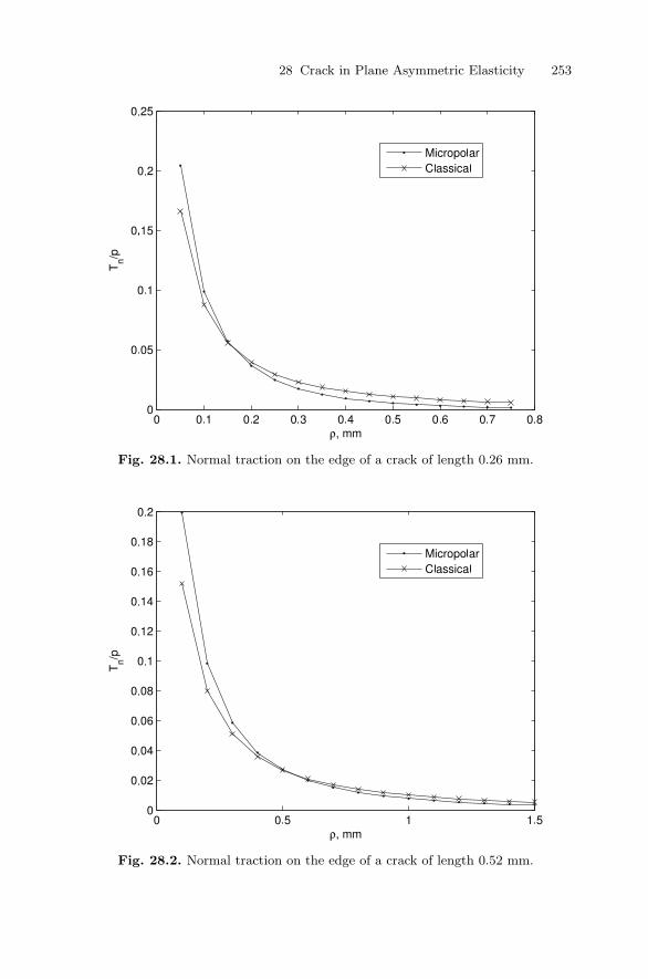
28 Crack in Plane Asymmetric Elasticity 253
Fig. 28.1. Normal traction on the edge of a crack of length 0.26 mm.
Fig. 28.2. Normal traction on the edge of a crack of length 0.52 mm.

254 E. Shmoylova, S. Potapenko, and L. Rothenburg
Fig. 28.3. Normal traction on the edge of a crack of length 0.75 mm.
of approximately three crack lengths from the tip of the crack, the effect ofthe crack on stresses is negligible, in agreement with Saint-Venant’s principle.
The results presented in Figures 28.1–28.3 may be compared with earlierinvestigations undertaken in the area of Cosserat solids. Nakamura and Lakes[NL88] performed an experimental study on stress concentrations aroundcracks in a human bone. They considered the same crack lengths as in thischapter. Later, Lakes et al. validated their results presented in [NL88] usingthe finite element method [LNB90]. However, it should be noted that a di-rect comparison with the results presented in [NL88] and [LNB90] does notseem feasible since our formulation of the crack problem is different from thatadopted in [NL88] and [LNB90], where a crack is considered to be a “blunt”notch, as in the approach of classical fracture mechanics [Sn69], in which acrack is usually modeled as a “squashed” ellipse of small eccentricity. The tipof the crack considered in [NL88] and [LNB90], therefore, is smooth, whereasin our study, the crack is represented by a piece of a plane curve whose edgeshave sharp corners. It has been found in [LNB90] that the difference in stressconcentrations near the crack edge between the classical and micropolar casefor a crack with a “blunt” tip may be up to 30% in the case when the cracklength is equal to 0.26 mm, and that for longer cracks, this difference is al-most negligible. The order of difference is in agreement with our results, butin [LNB90], the stress concentration near the crack tip in the micropolar case

28 Crack in Plane Asymmetric Elasticity 255
is lower than in the classical case. At a distance from the crack tip, the resultsobtained in [LNB90] are almost identical to the results of this investigation.
The explanation of discrepancies between our results and those presentedin [LNB90] in the vicinity of a crack tip lies in the crack geometry. If we con-sider a smooth contour such as an ellipse of small eccentricity as in [LNB90],then material particles can rotate under the applied load and generate couplestresses. Consequently, a part of the applied load is compensated by couplestresses and the resultant traction is reduced in comparison with the classi-cal case. When we consider a crack with a sharp tip, material particles gettrapped in the corner and cannot rotate; however, the load accumulated by thecouple stresses (due to continuity) is still present. Hence, the resultant stressin the vicinity of a sharp edge grows. When we move away from the corner,the particles gain back their ability to rotate and the load is redistributedbetween the stresses and the couple stresses, so the resultant traction startsdecreasing.
Indirect confirmation of our explanation may be found in [PL86] and[PSM04]. In [PL86], Park and Lakes performed an experimental investiga-tion of the torsion of a rectangular micropolar beam. The boundary of anytypical cross section of such a beam by a plane perpendicular to the genera-tors contains sharp corners. It has been found that the stress distribution onthe boundary of the beam cross section is significantly higher than in the casewhen microstructure is ignored. At the same time, the study by Potapenko etal. [PSM04], performed for an elliptic micropolar bar (in this case any typicalcross section of the bar is bounded by a smooth curve), shows that stressconcentrations on the boundary of the bar cross section may be up 15% lowerthan in the classical case. Similar conclusions may be drawn when we comparecracks with sharp and “blunt” tips in a micropolar medium.
28.6 Summary
In this chapter, we have shown that the method introduced by Shmoylovaet al. in [SPRb] may be applied to the investigation of stress distributionaround a crack with a sharp tip in a micropolar medium. We came to theconclusion that material microstructure has a significant effect on the stressdistribution around a crack, and demonstrated it by using the example of acrack in a human bone. The effect of material microstructure depends on thecrack length and crack geometry, and exercises the strongest influence in thevicinity of the crack tip.
References
[AlB93] Aliabadi, M.H., Brebbia, C.A.: Advances in Boundary Element Methodsfor Fracture Mechanics. Computational Mechanics Publ., Southampton,Boston; Elsevier, London-New York (1993).

256 E. Shmoylova, S. Potapenko, and L. Rothenburg
[AtL02] Atkinson, C., Leppington, F.G.: The effect of couple stresses on the tipof a crack. Internat. J. Solids Structures, 13, 1103–1122 (1977).
[BJ01] Bouyge, F., Jasiuk, I., Ostoja-Starzewski, M.: A micromechanicallybased couple-stress model of an elastic two-phase composite. Internat.J. Solids Structures, 38, 1721–1735 (2001).
[Br78] Brebbia, C.A.: The Boundary Element Method for Engineers. PentechPress, London (1978).
[CC00] Chudinovich, I., Constanda, C.: Variational and Potential Methods inthe Theory of Bending of Plates with Transverse Shear Deformation.Chapman & Hall/CRC, Boca Raton-London-New York-Washington, DC(2000).
[Er66] Eringen, A.C.: Linear theory of micropolar elasticity. J. Math. Mech.,15, 909–923 (1966).
[GKW03] Gaul, L., Kogl, M., Wagner, M.: Boundary Element Methods for Engi-neers and Scientists. Springer, Berlin-Heidelberg-New York (2003).
[JS04] Jasiuk, I., Ostoja-Starzewski, M.: Modeling of bone at a single lamellalevel. Biomech. Model. Mechanobiology, 3, 67–74 (2004).
[Lak82] Lakes, R.: Dynamical study of couple stress effects in human compactbone. J. Biomedical Engng., 104, 6–11 (1982).
[Lak95] Lakes, R.: Experimental methods for study of Cosserat elastic solids andother generalized elastic continua. In: Muhlhaus, H-B. (ed.), ContinuumModels for Materials with Microstructure. Wiley, New York (1995), pp.1–22.
[LNB90] Lakes, R., Nakamura, S., Behiri, J., Bonfield, W.: Fracture mechanics ofbone with short cracks. J. Biomech., 23, 967–975 (1990).
[MP02] Muhlhaus, H.-B., Pasternak, E.: Path independent integrals for Cosseratcontinua and application to crack problems. Internat. J. Fracture, 113,21–26 (2002).
[NL88] Nakamura, S., Lakes, R.: Finite element analysis of stress concentrationaround a blunt crack in a Cosserat elastic solid. Comput. Methods Appl.Mech. Engng., 66, 257–266 (1988).
[PL86] Park, H., Lakes, R.: Cosserat micromechanics of human bone: strainredistribution by a hydration sensitive constituent. J. Biomechanics, 19,385–397 (1986).
[PSM04] Potapenko, S., Schiavone, P., Mioduchowski, A.: Generalized Fourier se-ries solution of torsion of an elliptic beam with microstructure. Appl.Math. Lett., 17, 189–192 (2004).
[Sch96] Schiavone, P.: Integral equation methods in plane asymmetric elasticity.J. Elasticity, 43, 31–43 (1996).
[SPR06] Shmoylova, E., Potapenko, S., Rothenburg, L.: Weak solutions of theinterior boundary value problems of plane Cosserat elasticity. Z. Angew.Math. Phys., 57, 506–522 (2006).
[SPRa] Shmoylova, E., Potapenko, S., Rothenburg, L.: Weak solutions of theexterior boundary value problems of plane Cosserat elasticity. J. IntegralEquations Appl. (in press).
[SPRb] Shmoylova, E., Potapenko, S., Rothenburg, L.: Stress distribution arounda crack in plane micropolar elasticity. J. Elasticity (in press).
[Sn69] Sneddon, I.: Crack Problems in the Classical Theory of Elasticity. Wiley,New York (1969).

29
Euler–Bernoulli Beam with EnergyDissipation: Spectral Properties and Control
M. Shubov
University of New Hampshire, Durham, NH, USA;[email protected]
29.1 Statement of the Problem
We present several results on the problems associated with the Euler–Bernoullibeam model with dynamical nonconservative boundary conditions. A forcingterm, treated as a distributed control, is introduced into the equation govern-ing small transverse vibrations of a beam. The main question is the following:Can one provide an explicit formula for the control law in order to steer aninitial state to zero in a prescribed time interval of length T > 0? As weshow, the answer is affirmative for any T > 0 if certain conditions on the ini-tial state and force distribution function are satisfied; if these conditions arenot satisfied, then one has an approximate controllability (Theorems 6 and7 below). However, to give explicit formulas for the control laws, one needsthe following information: (i) detailed asymptotic and spectral results on thedynamics generator governing beam vibrations; (ii) facts about completeness,minimality (linear independence for an infinite number of vectors), and theRiesz basis property of the generalized eigenvectors of the dynamics generator(recall that a Riesz basis is a linear isomorphic image of an orthonormal basis,i.e., it is the mildest modification of an orthonormal basis); and (iii) results onsolvability of the corresponding moment problem that, in turn, requires someinformation on the basis property of nonharmonic exponentials in L2(0, T ).
We also present an interesting result on the nature of a semigroup for whichthe main operator, the dynamics generator, is an infinitesimal generator. Itis found that this semigroup is of a Gevrey class; i.e., differentiability of sucha semigroup is slightly weaker than that of an analytic semigroup (see [T89]and [TC90]).
Extensive research exists on the Euler–Bernoulli beam model in traditionalareas such as control, stability, and optimization for the model involving bothundamped and damped cases (see [CR82], [CKM87], [CLL98], [GWY05], and[R73]). However, one of the contemporary research directions is developing inthe field of unmanned aerial vehicles (UAV) in aeronautics. In particular, along-span, very light, flexible object in flight (high aspect-ratio “flying wing”

258 M. Shubov
configuration) can be considered as an elastic beam with both ends free, andboundary feedback stabilization of such a beam could be of great interestboth in control theory and in engineering practice (see [H90], [PHC00], and[PH04]).
Consider a linear model of the Euler–Bernoulli beam with a forcing term
ρ(x)htt(x.t) + (EI(x)hxx(x, t))xx = g(x)f(t), (x, t) ∈ (0, L) × R+, (29.1)
where h is the transverse displacement, ρ is the mass density, and EI is theflexural rigidity:
ρ ∈ C1[0, L], EI ∈ C2[0, L], ρ(x) > 0, EI(x) > 0, x ∈ [0, L]. (29.2)
We assume that the beam is clamped at the left end; i.e.,
h(0, t) = hx(0, t) = 0, t 0. (29.3)
The right-end conditions reflect shear feedback design for vibration suppres-sion [GWY05]
hxx(L) = 0, (EI(x)hxx(x, t))x|x=L = khxt(x, t)|x=L, (29.4)
with k being a positive parameter that can be changed in practice.The initial conditions are standard:
h(x, 0) = h0(x), ht(x, 0) = h1(x). (29.5)
In what follows, we assume that the force distribution function is g ∈L2(0, L); f will be called an admissible control function on the interval [0, T ]if f ∈ L2(0, T ).
29.1.1 Exact Controllability Problem
Let initial conditions (29.5) and T > 0 be given. Does there exist an admissiblecontrol f(t) on the interval [0, T ] such that the solution of problem (29.1)–(29.5) also satisfies the additional conditions at t = T
h(x, T ) = 0, ht(x, T ) = 0, x ∈ [0, L]? (29.6)
From now on, we will consider the case of a uniform beam with x ∈ [0, 1].Even though the asymptotic analysis of a differential equation with variablecoefficients is lengthy, the main results of this chapter remain essentially thesame in the nonuniform case.
Let H be the state space of the system; i.e., H is a Hilbert space of two-component vector-valued functions (h(x, t), ht(x, t))T obtained as a closureof the set of smooth, compactly supported functions U(x) = (u0(x), u1(x))T
in the norm (the superscript T means transposition)

29 Euler–Bernoulli Beam with Energy Dissipation 259
‖U‖2H =
∫ 1
0
[|u′′0(x)|2 + |u1(x)|2]dx.
Evidently, if U ∈ H, then u0(0) = u′0(0) = 0. Equation (29.1) and conditions
(29.2)–(29.5) (without a forcing term) define the following first order (in time)evolution problem:
Ut(x, t) = (LkU)(x, t), U |t=0 = (u00(x), u0
1(x))T , 0 x 1, t 0,
where the dynamics generator Lk is given by the matrix differential expression
Lk = −i
⎛⎝
0 1
− d4
dx4 0
⎞⎠ (29.7)
defined on the domain
D(Lk) =U ∈ H : u0 ∈ H4(0, 1), u1 ∈ H2(0, 1), u1(0) = u′
1(0) = 0,
u0(0) = u′0(0) = u′′
1(1) = 0, u′′′0 (1) = ku′
1(1) ,
where Hs(0, 1), s = 2, 4, are the standard Sobolev spaces [A75]. The adjointoperator L∗
k can be given by the same differential expression as (29.7), withthe following change in the domain:
D(L∗k) =U ∈ H : u0 ∈ H4(0, 1), u1 ∈ H2(0, 1), u1(0) = u′
1(0) = 0,
u0(0) = u′0(0) = u′′′
1 (1) = 0, u′′0(1) = ku1(1) .
29.2 Asymptotic and Spectral Properties of Operator Lk
29.2.1 Asymptotic Distribution of the Eigenvalues
Theorem 1. (i) Lk is an unbounded non-self-adjoint operator with a compactresolvent. Therefore, the spectrum of Lk consists of a countable set of normaleigenvalues (i.e., isolated eigenvalues, each of a finite algebraic multiplicity[GK96]) that can accumulate only at infinity.
(ii) (a) When k > 1, the following asymptotic representation holds for theeigenvalues as the number n of an eigenvalue tends to infinity:
λn = (πn)2 + iπn lnk + 1
k − 1− 1
4ln2 k + 1
k − 1+O(e−γn), n > 0,
where γ > 0 is an absolute constant. The spectrum is symmetric with respectto the imaginary axis; i.e., λ−|n| = −λn.
(b) When 0 < k < 1, the following asymptotic representation holds for theeigenvalues as the number n of an eigenvalue tends to infinity:
λn = π2
(n− 1
2
)2
+ iπ
(n− 1
2
)ln
1 − k
1 + k− 1
4ln2 1 − k
1 + k+O(e−γn), n > 0.

260 M. Shubov
29.2.2 Riesz Basis Property of the Generalized Eigenvectors
The set of the almost-normalized eigenvectors can be written in the form
Φn(x) =
( 1µ2
nϕn(x)
ϕn(x)
)
n∈Z
, ‖Φn‖H ≍ 1, (29.8)
where ϕn is an eigenfunction of the Sturm–Liouville problem that is equiv-alent to the spectral problem for Lk. The following approximation is valid asn → ∞ (µn =
√λn) :
ϕn(x) = sinµnx− cosµnx+ e−µnx +O(e−|n|).
Taking into account that µ−|n| = iµ|n|, as n → −∞, we obtain the approxi-mation
ϕ−|n|(x) = i(− sin(µ|n|x) + cos(µ|n|x)) − ie−µ|n|x +O(e−|n|).
As we know, the non-self-adjoint operator Lk may have a finite numberof multiple eigenvalues that could lead to a finite number of the associatevectors.
Theorem 2. The set of the generalized eigenvectors (eigenvectors and asso-ciate vectors together) of the operator Lk forms a Riesz basis for H. The setof the generalized eigenvectors of the adjoint operator L∗
k forms a biorthogonalRiesz basis (see [GK96], [S96], and [S00]).
29.2.3 Generation of a Gevrey-Class Semigroup
We now discuss the properties of a semigroup for which the operator (iLk)is an infinitesimal generator. This operator generates a strongly continuoussemigroup. Indeed, (iLk) is closed and its domain D(iLk) is dense in H. Theonly fact to be proved is that the resolvent R(λ, iLk) satisfies the estimate‖R(λ, iLk)n‖ M/(λ − ω)n, where M is an absolute constant and λ > ωwith some ω > 0 (see [P83] and [S06]). This estimate can be proved by usingthe spectral asymptotics and the spectral decomposition for the resolventoperator.
We now turn to the fact that the semigroup is of a Gevrey class. (Therelevant definition can be found in [T89], [TC90], and [S06].)
Theorem 3. A strongly continuous semigroup T (t) is of Gevrey class δ fort > t0 if it is infinitely differentiable for t ∈ (t0,∞) and if for every compactset K ⊂ (t0,∞) and each θ > 0, there exists a constant B = B(θ,K) such that‖T (n)(t)‖ Bθn(n!)δ for all t ∈ K and n = 0, 1, 2, . . . .
As one can see, “Gevrey regularity” involves bounds on the nth-orderderivatives, which are similar to (but somewhat weaker than) the bounds onthe nth-order derivatives for the case of an analytic semigroup [P83]. Themain result of this section is included in the next assertion.

29 Euler–Bernoulli Beam with Energy Dissipation 261
Theorem 4. The semigroup generated by the operator Lk is of Gevrey classδ > 1/2.
The detailed proof can be found in [S06].
29.3 Moment Problem and Controllability Results
29.3.1 Some Known Results on Nonharmonic Exponentials
To formulate the solution of the control problem , we need some information onthe properties of nonharmonic exponentials (see [HNP81], [Y80], and [AI95]).Let
P =exp
(iλn t
)n∈Z
,
where λnn∈Z is the spectrum of Lk. The following statement is valid for P:
Theorem 5. For any T > 0, (i) the set of nonharmonic exponentials P isnot complete in L2(0, T ), and (ii) this set forms a Riesz basis for its closedlinear span in L2(0, T ).
Let T > 0, and let E (P, T ) denote the smallest closed subspace in L2(0, T )containing P. As is well known [FR71], E (P, T ) is a proper subspace ofL2(0, T ) if and only if
∑n∈Z
1|λn| < ∞, which is our case. It is also known
that if Pn ≡λn |k = n
, then E (Pn, T ), then the smallest closed sub-
space in L2(0, T ) containing Pndoes not include exp(iλnt). In this case, usingstandard arguments from Hilbert space theory, one can show that there is aunique function τn(t) ∈ E(Pn, T ) that is closest to the function exp(iλnt) inthe L2(0, T )-norm. If
(dn(T ))2 =
∫ T
0
(eiλnt − τ(t))2dt,
then the set
ψn(t) =eiλnt − τn(t)
(dn(T ))2, n ∈ Z,
is a biorthogonal set for P in L2(0, T ). Obviously, since the set P is notcomplete in L2(0, T ), the biorthogonal set is not unique. However, the set
ψnn∈Z is called the optimal biorthogonal set for P. Suppose that ψnn∈Z
is any other biorthogonal vector for P in L2(0, T ). It is easily verified that
ψn = ψn + ϕn and ϕn ∈ E(P, T )⊥, n ∈ Z; hence, ‖ψn‖L2(0,T ) ‖ψn‖L2(0,T ),n ∈ Z, which yields ‖ψn‖L2(0,T ) = (dn (T ))−1.
Since P is a Riesz basis for E(P, T ), the biorthogonal family ψnn∈Z isalso a Riesz basis for E(P, T ).

262 M. Shubov
29.3.2 Moment Problem
Let G(x) = (0, g(x), 0, 0)T ∈ H, where g(x) is the force profile function from(29.1). Then, from (29.1)–(29.5), we obtain the following representation of theinitial problem:
Ut(x) = i(LkU)(x) + f(t)G(x), U(x, 0) = F0(x). (29.9)
Let us expand the solution of (29.9) with respect to the Riesz basis of thegeneralized eigenvectors of the operator Lk (29.8):
U(x, t) =∑
n∈Z
an(t) Φn(x), x ∈ (0, 1), t 0. (29.10)
We use through numeration for the generalized eigenvectors making no dif-ference between the eigenvectors and associate vectors of Lk. We also expandthe functions G(·) and F0(·) with respect to the same Riesz basis:
G(x) =∑
n∈Z
gn Φn(x), F0(x) =∑
n∈Z
ϕn Φn(x),∑
n∈Z
(|gn|2 + |ϕn|2
)< ∞.
(29.11)Substituting (29.10) and (29.11) into (29.9), we obtain an infinite sequence ofthe initial-value problems
(an(t))t = iλnan(t) + gnf(t), an(0) = ϕn, n ∈ Z. (29.12)
Solving problems (29.12) for an(t), we rewrite representation (29.10) in theform
U(x, t) =∑
n∈Z
[ϕn e
iλnt + gn
∫ t
0
eiλn(t−τ)f(τ)dτ
]Φn(x). (29.13)
Our main question is the following: Is there a moment T > 0 such thatU(x, T ) = 0? From (29.13) and the Riesz basis property of Φnn∈Z, we findthat U(x, T ) = 0 if and only if the following infinite system of equations hasa solution f ∈ L2(0, T ) :
ϕn + gn
∫ T
0
e−iλnτ f(τ)dτ = 0, n ∈ Z. (29.14)
The problem of finding a solution of (29.14) is known as the moment problem(see [Y80] and [Z91]). To solve it, we will use the properties of nonharmonicexponentials.
29.3.3 Exact and Approximate Controllability
We are now in a position to present our results on exact controllability [S07].

29 Euler–Bernoulli Beam with Energy Dissipation 263
Theorem 6. (i) Suppose that
gn = 0 for all n ∈ Z. (29.15)
The following statements are valid.(a) System (29.9) is controllable on the time interval [0, T ] with any T > 0
if and only if
γn ≡ ϕn/gnn∈Z∈ ℓ2(Z), i.e.,
∑
n∈Z
|γn|2 < ∞. (29.16)
(b) The desired control function f , which brings the system to the zerostate on the time interval [0, T ], T > 0, can be defined by the formula
f(t) = −∑
n∈Z
γn ψn(t), (29.17)
where ψn are the functions biorthogonal to the corresponding nonharmonic ex-ponentials. There exist infinitely many control functions from L2(0, T ). How-
ever, f defined by (29.17) has the minimal norm; i.e., if another function fbrings the system to rest in the same time T , then
‖f‖L2(0,T ) ‖f‖L2(0,T ).
(ii) Assume that (29.15) is not satisfied, and let R = n ∈ Z : gn = 0.Let γn be defined by (29.16) only for n ∈ Z\R, and let S = n ∈ Z : ϕn = 0.Then the following statements hold:
(a) The system is controllable in time T > 0 if and only if R ⊆ S and
∑
n∈Z
|γn|2 < ∞.
(b) The desired control function is not unique and can be given by theformula
f(t) = −[ ∑
n∈Z\S
γn ψn(t) +∑
m∈R
bm ψm(t)
],
where bm ∈ C are arbitrary coefficients such that∑
m∈R
|bm|2 < ∞.
(c) If the set R\(R⋂S) is not empty, then the system is not controllable
in any time.
Remark 1. The formulas for the basis functions ψn(t) that are biorthogonal tothe basis of the nonharmonic exponentials are known to be very complicatedand can be given in terms of the truncated Blaschke product.

264 M. Shubov
Theorem 7. (Approximate Controllability) Suppose that condition (29.16) isnot valid, but that
γnn∈Z∈ lq(Z) for some q ∈ (2,∞], i.e.,
∑
n∈Z
|γn|q < ∞, (if 2 < q < ∞) or supn∈Z
|γn| < ∞ (if q = ∞).
Then for any ǫ > 0, there exists N such that for the control function
fN (t) =∑
|n|N
γn ψn(t),
the following estimate is valid:
‖U(·, T )‖H ǫ for T > 0.
However, ‖fN‖L2(0,T ) → ∞ as N → ∞.
Acknowledgement. The author is grateful to Irena Lasiecka for important infor-mation on Gevrey-class semigroups. Partial support from the NSF award DMS #0604842 is highly appreciated.
References
[A75] Adams, R.A.: Sobolev Spaces. Academic Press, New York (1975).[AI95] Avdonin, S.A., Ivanov, S.A.: Families of Exponentials. The Method of
Moments in Controllability Problems for Distributed Parameter Systems.Cambridge University Press, Cambridge (1995).
[CR82] Chen, G., Russell, D.L.: A mathematical model for linear elastic systemswith structural damping. Quart. Appl. Math., 39, 433–454 (1982).
[CKM87] Chen, G., Krantz, S.G., Ma, D.W., Wayne, C.E., West, H.H.: The Euler-Bernoulli beam equations with boundary energy dissipation. In: OperatorMethods for Optimal Control Problems. Marcel Dekker, New York (1987),pp. 67–96.
[CLL98] Chen, S., Liu, K., Liu, Z.: Spectrum and stability for elastic systems withglobal or local Kevin–Voigt damping. SIAM J. Appl. Math., 59, 651–668(1998).
[FR71] Fattorini, H.O., Russell, D.L.: Exact controllability theorems for linearparabolic equations in one space dimension, Arch. Rational Mech. Anal.,43, 272–292 (1971).
[GK96] Gohberg, I.Ts., Krein, M.G.: Introduction to the Theory of Linear Non-selfadjoint Operators. AMS, Providence, RI (1996).
[GWY05] Guo, B.–Z., Wang, J.–M., Yung, S.–P.: On the C0-semigroup genera-tion and exponential stability resulting from a shear force feedback on arotating beam. Systems Contr. Lett., 54, 557–574 (2005).
[H90] Hodges, D.H.: A mixed variational foundation based on exact intrinsicequations for dynamics of moving beams. Internat. J. Solids Structures,26, 1253–1273 (1990).

29 Euler–Bernoulli Beam with Energy Dissipation 265
[HNP81] Hruschev, S.V., Nikol’skii, N.K., Pavlov, B.S.: Unconditional Basesof Exponentials and Reproducing Kernels. Springer, Berlin-Heidelberg(1981), pp. 214–335.
[PHC00] Patil, M.J., Hodges, D.H., Cesnik, C.E.S.: Nonlinear aeroelastic analysisof complete aircraft in subsonic flow. J. Aircraft, 37, 753–760 (2000).
[PH04] Patil, M.J., Hodges, D.H.: On the importance of aerodynamic and struc-tural geometrical nonlinearities in aeroelastic behavior of high aspect-ratio wings. J. Fluids Structures, 19, 905–915 (2004).
[P83] Pazy, A.: Semigroups of Linear Operators and Applications to PartialDifferential Equations. Springer, New York (1983).
[R73] Russel, D.L.: A unified boundary controllability theory for hyperbolicand parabolic partial differential equations. Stud. Appl. Math., 52, 189–211 (1973).
[S96] Shubov, M.A.: Riesz basis property of eigenfunctions of nonselfadjointoperator pencils generated by the equation of nonhomogeneous dampedstring. Integral Equations Oper. Theory, 25, 289–328 (1996).
[S00] Shubov, M.A.: Riesz basis property of root vectors of nonselfadjoint op-erators generated by radial damped wave equations. Adv. DifferentialEquations, 5, 623–656 (2000).
[S06] Shubov, M.A.: Generation of Gevrey class semigroup by non-selfadjointEuler–Bernoulli beam model. Math. Methods Appl. Sci., 29, 2181–2199(2006).
[S07] Shubov, M.A.: Exact controllability of nonselfadjoint Euler–Bernoullibeam model via spectral decomposition method. IMA J. Math. ControlInf. (in press).
[T89] Taylor, S.W.: Gevrey regularity of solutions of evolution equations andboundary controllability. PhD Thesis, University of Minnesota, Min-neapolis (1989).
[TC90] Triggiani, R., Chen, S.: Gevrey class semigroups arising from elastic sys-tems with gentle dissipation: the case 0 < α < 1/2. Proc. Amer. Math.Soc., 110, 401–415 (1990).
[Y80] Young, R.M.: Introduction to Nonharmonic Fourier Series. AcademicPress, New York (1980).
[Z91] Zwaan, M.: Moment Problems in Hilbert Space with Applications to Mag-netic Resonance Imaging. Centrum voor Wiskunde en Informatica, CWITRACT (1991).


30
Correct Equilibrium Shape Equation ofAxisymmetric Vesicles
N.K. Vaidya1, H. Huang1, and S. Takagi2
1 York University, Toronto, ON, Canada; [email protected],[email protected]
2 University of Tokyo, Japan; [email protected]
30.1 Introduction
Under favorable conditions, lipid molecules consisting of hydrophobic tail andhydrophilic head groups, self-assemble to form vesicles in an aqueous mediumwith a lipid bilayer separating the inner and outer solutions [Ino96], [Kom96].Vesicles have been attracting enormous attentions because of their biologicalsignificance with numerous applications such as drug delivery and targeting,medical imaging, catalysis, etc. [KR96], [Zan96]. It is recognized that theequilibrium shape of the vesicle is determined by minimizing a shape energygiven by the spontaneous-curvature model of Helfrich [Hel73], [OH89]:
F =1
2kb
∮(c1 + c2 − c0)
2dA + kG
∮c1c2dA + λ
∮dA + ∆P
∫dV. (30.1)
Here dA, dV , and kb are the surface area element, volume element, and thebending rigidity, respectively; c1 and c2 denote the two principal curvaturesand c0 denotes the spontaneous curvature, which takes the possible asymme-try of the bilayer into account; λ and ∆P are Lagrangian multipliers usedto incorporate the constraints of constant area and constant volume, respec-tively. Physically, λ and ∆P can be interpreted as the tensile stress and pres-sure difference, respectively. For vesicles with the same topological forms, theGaussian curvature term kG
∮c1c2dA can be dropped from (30.1).
For vesicles with axisymmetric equilibrium shapes, four different ap-proaches have been used to derive the shape equation in the literature.
A1. In Ou-Yang and Helfrich [OH89], a general shape equation was derived byallowing the variation of the functional F only in the normal direction ofthe membrane surface. The axisymmetric shape equation can be obtainedby applying the axisymmetric condition.
A2. This approach is similar to A1, allowing variation only in the normal direc-tion. The difference is that variation is carried out after the axisymmetriccondition is applied [HO93].

268 N.K. Vaidya, H. Huang, and S. Takagi
A3. Again, functional F is written in the axisymmetric form first. The calcu-lus of variation is performed without the restriction in the normal direc-tion [MFR91], [Pet85].
A4. This approach is similar to A3. However, the arc-length is used as theprimary variable, instead of the distance to the axis of symmetry [SBL91],[Sef66].
Both A1 and A2 generate the same equation. The shape equations producedby A3 and A4, however, are slightly different, as pointed out in [HO93]. Inan attempt to remove the confusion, it was shown in [ZL93] that the shapeequations in A1 and A3 are related. However, due to the coordinate singular-ity, this relationship does not necessarily imply equivalence [BP04], [Poz03].This was confirmed in [NOO93] with the help of an analytical expression ofa circular biconcave discoid (the shape of red blood cells). In addition, byconsidering the 2D limit, it was shown that the equations derived from A3and A4 are erroneous since they do not recover the correct equation, whereasthe equation from A1 and A2 gives the correct limit [BP04], [Poz03]. Otherspecial solutions have also been used to validate or invalidate the equivalenceof the shape equations [HO93], [NOO93]. The most satisfactory discussionabout these issues has been presented in [JS94], in which it was shown thatthe same equation can be obtained by A4 and A1. Their main conclusion isthat an additional equation has to be introduced for the Hamiltonian (i.e.,constant Hamiltonian), which can be maintained by proper treatment of theboundary conditions. However, this idea of treatment of the boundary condi-tion does not work for fixed integral limits (i.e., constant total contour length)and the validity of the argument was questioned by [BP04], [Poz03]. There-fore, it is still not clear whether it is necessary to restrict the variation in thenormal direction, as suggested in [OH89].
In this chapter, we show that the same shape equation in A1 and A2 canbe obtained without restricting the variation in the normal direction. We fur-ther prove that a slight modification of A3 produces the correct equation. Aslong as a geometric condition is satisfied (explicitly or implicitly), the varia-tion does not have to be in the normal direction, contrary to the argumentin [HO93]. To show the equivalence of equations by A1 and A4, [JS94] alsosuggested similar types of geometric conditions. However, they and others fol-lowing their arguments have not implemented these conditions in their laterworks [DBS03], [JL96] when attempting to get the axisymmetric shape equa-tions. Our result (correct shape equation by modification of A3) suggests thatwhen A4 is used, apart from the extra Hamiltonian condition, the geometriccondition should also be imposed properly to get the correct shape equations.
The rest of the chapter is organized as follows. In Section 30.2, we presentthe equations obtained using A1–A3 in the literature. In Section 30.3, weshow that the correct equation can be obtained by taking the variation in thedirection perpendicular to the axis of symmetry. Furthermore, by imposingthe geometric condition implicitly in the action form of the energy functional,

30 Equation of Axisymmetric Vesicles 269
we show that A3 can produce exactly the same equation as A1 (and A2).Various topological shapes of vesicles are discussed in Section 30.3.4, and wepresent our conclusions in Section 30.4.
30.2 Shape Equation
We consider vesicles of axisymmetric shape with the axis of symmetry alongthe z-axis. We denote the arc length of the contour, the distance to the sym-metric axis, and the angle made by the tangent to the contour with the planeperpendicular to the axis of symmetry by s, ρ, and ψ, respectively (see Figure30.1(a).
(a) (b)
Fig. 30.1. (a) Schematic diagram of the axisymmetric vesicle. (b) The variation inthe direction perpendicular to the axis of symmetry (i.e., in ρ-direction). AB = dsis the segment in the original generating curve, CD is the corresponding segmentin the curve deduced by the variation δρ in the ρ-direction, and the dashed curve isthe curve deduced by moving the original curve from A to C.
Using A1, that is, substituting the mean curvature
H = −(c1 + c2)/2 = −(1/2)[cos ψ(dψ/dρ) + sinψ/ρ]
and the Gaussian curvature
K = c1c2 = cos ψ sin ψ(1/ρ)(dψ/dρ)
in the general shape equation derived by Ou-Yang and Helfrich [OH89], weobtain the shape equation as (see [BP04], [HO93], [NOO93], [Poz03], and[ZL93])

270
cos3 ψd3ψ
dρ3= 4 sin ψ cos2 ψ
d2ψ
dρ2
dψ
dρ− cos ψ(sin2 ψ − 1
2cos2 ψ)
(dψ
dρ
)3
+7 sin ψ cos2 ψ
2ρ
(dψ
dρ
)2
− 2 cos3 ψ
ρ
d2ψ
dρ2
+
(c20
2− 2c0 sin ψ
ρ+
sin2 ψ
2ρ2+
λ
kb− sin2 ψ − cos2 ψ
ρ2
)cos ψ
dψ
dρ
+∆P
kb+
λ sin ψ
kbρ− sin3 ψ
2ρ3+
c20 sin ψ
2ρ− sin ψ cos2 ψ
ρ3. (30.2)
The axisymmetric shape equation generated by A3, in which axisymmetricexpressions for curvatures are used in (30.1) and the Euler–Lagrange equationis obtained, is (see [MFR91] and [Pet85])
H = 0,
where
H = cos2 ψd2ψ
dρ2− sin ψ cos ψ
2
(dψ
dρ
)2
− sin ψ
2ρ2 cos ψ− sin ψ cos ψ
2ρ2− c2
0 sin ψ
2 cos ψ
+cos2 ψ
ρ
dψ
dρ− c0 sin2 ψ
ρ cos ψ− ∆Pρ
2kb cos ψ− λ sin ψ
kb cos ψ. (30.3)
The shape equation based on A4 is obtained in the same way [JS94], [SBL91],[Sef66].
30.3 Equivalence of the Shape Equations
Equation (30.3) has been obtained without any reference to the z-coordinate.Therefore, ψ(ρ) varies over a larger class of functions, and the extremalfunction, which minimizes the energy functional, may not be admissible. Infact, the coordinates z(s) and ρ(s) have to satisfy the geometric relationsdρ/ds = cos ψ and dz/ds = − sin ψ, which give the geometric relation in theparameter ρ as
dz
dρcos ψ + sinψ = 0. (30.4)
In what follows, we show that the correct shape equation can be obtained ifthis geometric condition is imposed explicitly or implicitly. We will demon-strate this fact by using two different approaches.
30.3.1 Variation in the ρ-Direction
We now derive the shape equation for axisymmetric vesicles by taking the vari-ation of the axisymmetric energy functional. The method used here is similar
N.K. Vaidya, H. Huang, and S. Takagi

30 Equation of Axisymmetric Vesicles 271
to A2 [HO93], but the variation is performed along the direction perpendic-ular to the axis of symmetry (i.e., the ρ-direction) and the correspondinginduced variations in ψ and s are obtained by using the geometric relationsdρ/ds = cos ψ and dz/ds = − sin ψ. The method used here is similar to themethod used to find the equation of geodesics in Riemannian geometry bymeans of the variational method [HO93], [Spi79].
We start with the axisymmetric shape energy functional with parameters
Fs = π
∫ [kbρ
(dψ
ds+
sinψ
ρ− c0
)2
+∆Pρ2 sinψ + 2λρ
]ds
and introduce an arbitrary parameter t to get
Fs = π
∫L(ρ(t), ψ(t), ψ(t), s(t)
)dt,
where
L(ρ(t), ψ(t), ψ(t), s(t)
)=
kbρ(ψ)2
s+kbs sin2 ψ
ρ+ kbρc
20s− 2kbc0ρψ
+2λρs+∆Pρ2 sinψs. (30.5)
Note that the terms 2kbψ sinψ and −2kbc0s sinψ have been neglected in (30.5)as they do not contribute to the shape equation [HO93].
Let δρ be an infinitesimal variation along the ρ-direction so that the vari-ation along the z-direction is δz = 0 (see Figure 30.1(b)). The geometricrelation dρ = cosψds gives
− sinψds(δψ) + cosψδds = δdρ. (30.6)
Similarly, the geometric relation dz = − sinψds, given that dδz = δdz due tothe independence of the operators d and δ, yields
cosψds(δψ) + sinψδ(ds) = 0. (30.7)
Solving (30.6) and (30.7) for δψ and δ(ds), we get
δψ = − sinψδdρ
ds, δ(ds) = cosψδdρ, δψ = − d
dt
(sinψδdρ
ds
), δs =
cosψδdρ
dt.
The shape equation is determined by the variational equation δFs = 0,which leads to
∫ [∂L
∂ρδρ+
∂L
∂ψδψ +
∂L
∂ψδψ +
∂L
∂sδs
]dt = 0. (30.8)
Using expressions for δψ, δψ, and δs in (30.8), and performing integration byparts and simplification, we obtain the shape equation

272
∂L
∂ρ+
d
dt
(sin ψ
s
∂L
∂ψ
)− d
dt
(sin ψ
s
d
dt
∂L
∂ψ
)− d
dt
(cos ψ
∂L
∂s
)= 0. (30.9)
We use (30.5) in (30.9) and consider ρ as a parameter by taking t = ρ. Then,using ψ = dψ/dρ, s = ds/dρ = 1/ cos ψ, and ρ = 1 along with their higherderivatives in the resulting equation, we obtain (30.2), which is also the shapeequation derived in the literature from A2. Therefore, we have shown that thevariation does not have to be in the normal direction, and that the variationin other directions can also produce the same shape equation if the inducedvariations in the other variables are obtained from the geometric relationsdρ/ds = cos ψ and dz/ds = − sin ψ. We note that the approach outlined herebreaks down when the surface is perpendicular to the axis of symmetry. Wenow move on to a more general approach.
30.3.2 The Method of Lagrange Multiplier
We include the geometric condition (30.4) in the action form of the shapeenergy functional via an additional Lagrange multiplier η as follows:
F = π
∫L
(ρ, ψ(ρ), z(ρ), η(ρ),
dψ
dρ,dz
dρ
)dρ,
where the Lagrangian L is
L =kbρ
cosψ
(dψ
dρcosψ +
sinψ
ρ− c0
)2
+∆Pρ2 sinψ
cosψ+
2λρ
cosψ
+η
(dz
dρcosψ + sinψ
).
This gives the Euler–Lagrange equations
H =η
2kbρ, (30.10)
dz
dρ= − sinψ
cosψ, (30.11)
cosψdη
dρ= η sinψ
dψ
dρ. (30.12)
We rewrite (30.10) as η = η(ρ, ψ, dψ/dρ, d2ψ/dρ2
)and find the expression
for dη/dρ, then substitute the expressions for η and dη/dρ in (30.12). Afterlengthy mathematical manipulations, we obtain (30.2), which is the equationgenerated by A1 (and A2).
This suggests that the discrepancy in the shape equations obtained by dif-ferent approaches in the literature occurs when the geometric relation (30.4)is not imposed. A3 can produce the same equation as A1 (and A2) as long asthe geometric relation (30.4) is preserved when the variation is performed. In
N.K. Vaidya, H. Huang, and S. Takagi

30 Equation of Axisymmetric Vesicles 273
the situation when ψ can vary independently without taking z into considera-tion, the geometric condition is not necessary. Furthermore, if the variation iswith respect to the normal displacement, as in A1 and A2, ρ and z are variedproportionately so that the geometric relation is implicitly preserved.
30.3.3 Relationship Between the Shape Equations
Equation (30.12) can be expressed as d(η cos ψ)/dρ = 0, which, by (30.10),leads to d(ρH cos ψ)/dρ = 0. We note that this relation differs from the equa-tion in [ZL93]; i.e., (1/ρ)[d(ρH cos ψ)/dρ] = 0, which has an extra factor 1/ρ.Not having 1/ρ avoids the singularity at ρ = 0, which removes the doubt onthe validity of the conclusion in [ZL93], as pointed out in [BP04] and [Poz03].Integrating once yields η cos ψ = 2kbρH cos ψ = C, where C is an integrat-ing constant. Obviously, C = 0 does not necessarily lead to H = 0 unlessρ cos ψ = 0. Therefore, (30.2) and (30.3) are equivalent if and only if η = 0,which is relatively easy to verify.
30.3.4 Vesicles with Distinct Topological Shapes
It has been pointed out in the literature that the shape equations obtainedusing different approaches are equivalent only for spherical vesicles. We nowdemonstrate this by observing the value of the Lagrange multiplier η used inour approach.
Spherical Vesicles
For spherical vesicles, ρ = r0 sin ψ, (30.2) leads to ∆Pr30 + 2λr2
0 + kbc20r
20 −
2kbc0r0 = 0 and (30.10)–(30.12) yield
∆Pr30 + 2λr2
0 + kbc20r
20 − 2kbc0r0 + η cot ψ csc ψr0 = 0.
Since these two conditions are identical, we have η = 0. Thus, (30.3) is equiv-alent to (30.2) for spherical vesicles. This is due to the fact that we do notneed to impose any constraint on z and its derivatives, which allows ψ to varyfreely.
Cylindrical Vesicles
We now assume that the vesicle is of cylindrical shape, which is given by theequations ρ = r0, ψ = π/2. Substituting this in (30.2) and in (30.10)–(30.12),we can verify that for this cylindrical vesicle equation to be a solution of both(30.2) and (30.10)–(30.12), we require that
C = ∆Pr0 (2 − r0)+2λr0
(1
r0− 1
)+c20kbr0
(1
r0− 1
)+2kbc0−
kb
r0
(1
r0+ 1
).
274
Since C = 0 and cosψ = 0, η cannot be zero. To obtain the cylindricalvesicle, we need to have infinite slope dz/dρ (= − sin ψ/ cos ψ), which mustbe maintained when the variation is performed. Hence, (30.3) and (30.2) arenot equivalent for cylindrical vesicles.
Toroidal Vesicles
Similarly, a vesicle of perfect torus shape given by ρ = x+ sin ψ, where 1/x isthe ratio of its generating radii, can be a solution of both (30.2) and (30.10)–(30.12) only if C = 2kb(1 + 2c0). Thus, η = 0 only if c0 = −1/2. However,based on experiments performed in [FMB92], [MBB91], and [MB91] and thetheoretical result in [Wil82], in general [HO93] c0 = −1/2. Therefore, η = 0and (30.3) is not equivalent to (30.2) for toroidal vesicles.
As a simple observation, we offer the following explanation. To have avesicle of perfect torus shape, we need to have vanishing slope of the curvez = z(ρ) at the point ρ = x (i.e., (dz/dρ)|ρ=x = 0). Because of this condition,ψ cannot vary without taking z into consideration.
Circular Biconcave Discoids
In [NOO93], the authors showed that ψ = arcsin[ρ(c0 ln ρ+b)] with a constantb is a solution of (30.2) under the condition ∆P = λ = 0. This solution withc0 < 0 represents a circular biconcave discoid, the shape of the red blood cell(RBC). For this vesicle to be a solution of (30.10)–(30.12) under the condition∆P = λ = 0, we require that η = 4kbc0/(
√1 − ρ2(c0 ln ρ + b)2). The nonzero
η indicates that (30.3) is not equivalent to (30.2), unless c0 = 0.When c0 = 0, the biconcave vesicle z = z(ρ) has a local extreme value;
i.e., dz/dρ = 0 at ρ = exp(−b/c0). Thus, ψ cannot vary independently. Whenc0 = 0, the biconcave vesicle becomes spherical with b = 1/r0; thus, η = 0,and (30.3) and (30.2) become equivalent.
30.4 Conclusion
We have introduced two new approaches for deriving the equilibrium shapeequation for axisymmetric vesicles. We have shown that as long as the ge-ometric relation dz/dρ = − tanψ is maintained in performing the calculusof variations, both approaches produce the correct shape equation. We havealso shown that the variation does not have to be in the normal direction.Furthermore, by imposing the geometric condition as a Lagrange multiplier,we established a simple relationship between the two distinct shape equa-tions derived previously in the literature. Using this relationship, it becomesa straightforward exercise to verify the equivalence of the shape equation usingexplicit shape solutions.
N.K. Vaidya, H. Huang, and S. Takagi

30 Equation of Axisymmetric Vesicles 275
Acknowledgement. Part of this research was supported by the Natural Science andEngineering Research Council (NSERC) of Canada. One of the authors (HH) alsowishes to thank Japan Society for the Promotion of Sciences (JSPS) for providinga visiting fellowship that enabled him to carry out a part of this research.
References
[BP04] Blyth, M.G., Pozrikidis, C.: Solution space of axisymmetric capsules en-closed by elastic membranes. Eur. J. Mech. A/Sol., 23, 877–892 (2004).
[DBS03] Derganc, J., Bozic, B., Svetina, S., Zeks, B.: Equilibrium shape of ery-throcytes in rouleau formation. Biophys. J., 84, 1486–1492 (2003).
[FMB92] Fourcade, B., Mutz, K., Bensimon, D.: Experimental and theoretical studyof toroidal vesicles. Phys. Rev. Lett., 68, 2551–2554 (1992).
[Hel73] Helfrich, W.: Elastic properties of lipid bilayers—theory and possible ex-periments. Z. Naturforsch., 28c, 693 (1973).
[HO93] Hu, J.-G., Ou-Yang, Z.-C.: Shape equations of the axisymmetric vesicles.Phys. Rev. E, 47, 461–467 (1993).
[Ino96] Inoue, T.: Interaction of surfactants with phospholipid vesicles. In: Vesi-cles. Marcel Dekker, New York (1996), pp. 152–195.
[JL96] Julicher, F., Lipowsky, R.: Shape transformations of vesicles with in-tramembrane domains. Phys. Rev. E, 53, 2670–2683 (1996).
[JS94] Julicher, F., Seifert, U.: Shape equations for axisymmetric vesicles: a clar-ification. Phys. Rev. E, 49, 4728–4731 (1994).
[Kom96] Komura, S.: Shape fluctuations of vesicles. In: Vesicles. Marcel Dekker,New York (1996), pp. 198–236.
[KR96] Kunieda, H., Rajagopalan, V.: Formation and structure of reverse vesicles.In: Vesicles. Marcel Dekker, New York (1996), pp. 80–103.
[MFR91] Miao, L., Fourcade, B., Rao, M., Wortis, M.: Equillibrium budding andvesiculation in the curvature model of fluid lipid vesicles. Phys. Rev. A,43, 6843–6856 (1991).
[MBB91] Mutz, M., Bensimon, D., Birenne, M.J.: Wrinkling transition in partiallypolymerized vesicles. Phys. Rev. Lett., 67, 923–926 (1991).
[MB91] Mutz, M., Bensimon, D.: Observation of toroidal vesicles. Phys. Rev. A,43, 4525–4527 (1991).
[NOO93] Naito, H., Okuda, M., Ou-Yang, Z.-C.: Counterexample to some shapeequations for axisymmetric vesicles. Phys. Rev. E, 48, 2304–2307 (1993).
[OH89] Ou-Yang, Z.-C., Helfrich, W.: Bending energy of vesicle membranes: gen-eral expressions for the first, second and third variation of the shape en-ergy and applications to spheres and cylinders. Phys. Rev. A, 39, 5280–5288 (1989).
[Pet85] Peterson, M.: An instability of the red blood shape. J. Appl. Phys., 57,1739–1742 (1985).
[Poz03] Pozrikidis, C.: Shell Theory for Capsules and Cells. Modeling and Sim-ulation of Capsules and Biological Cells. Chapman & Hall/CRC, BocaRaton, FL (2003), pp. 35–101.
[SBL91] Seifert, U., Berndl, K., Lipowsky, R.: Shape transformations of vesicles:phase diagram for spontaneous-curvature and bilayer-coupling models.Phys. Rev. A, 44, 1182–1202 (1991).
276
[Sef66] Seifert, U.: Vesicles of toroidal topology. Phys. Rev. Lett., 66, 2404–2407(1991).
[Spi79] Spivak, M.: A Comprehensive Introduction to Differential Geometry. Pub-lish or Perish, Berkeley (1997).
[Wil82] Willmore, T.J.: Total Curvature in Riemannian Geometry. Horwood,Chichester (1982).
[Zan96] Zanten, Z.H.V.: Characterization of vesicles and vesicular dispersions viascattering techniques. In: Vesicles. Marcel Dekker, New York (1996), pp.240–294.
[ZL93] Zheng, W., Liu, J.: Helfrich shape equation for axisymmetric vesicles asa first integral. Phys. Rev. E, 48, 2856–2860 (1993).
N.K. Vaidya, H. Huang, and S. Takagi

31
Properties of Positive Solutions of theFalkner–Skan Equation Arising in BoundaryLayer Theory
G.C. Yang1, L.L. Shi1, and K.Q. Lan2
1 Chengdu University of Information Technology, Sichuan, P.R. China;[email protected], [email protected]
2 Ryerson University, Toronto, ON, Canada; [email protected]
31.1 Introduction
We consider the well-known Falkner–Skan equation⎧⎪⎨⎪⎩
f ′′′(η) + f(η)f ′′(η) + λ[1 − (f ′)2(η)] = 0 on η ∈ (0,∞),
f(0) = f ′(0) = 0, f ′(∞) = 1,
0 < f ′(η) < 1 for η ∈ (0,∞),
(31.1)
which is used to describe the steady two-dimensional flow of a slightly vis-cous incompressible fluid past a wedge-shaped body of angle related to λπ/2,where η is the similarity boundary layer ordinate, f(η) is the similarity streamfunction, and f ′(η) and f ′′(η) are the velocity and shear stress, respectively.If λ ∈ [−2, 0], the corresponding flow is called a corner flow and if λ ∈ [0, 2],the flow is a wedge flow. We refer to [Na79] and [SG00] for a more detailedphysical interpretation of (31.1).
It is well known that there exists λ∗ < 0 such that (31.1) has at leastone solution for each λ ≥ λ∗ and no solutions for λ < λ∗. Moreover, thecondition 0 < f ′(η) < 1 for η ∈ (0,∞) can be replaced by f ′′(η) > 0 forη ∈ (0,∞) (see [LY07] and the references therein). An open problem leftin [LY07] is what is exactly λ∗? A well-known numerical result shows thatλ∗ = −0.1988 (see [BS66], [LL67], and [RW89]). We refer to [AO02], [Cop60],[Har02], [Har72], [Has71], [Has72], [Tam70], [WG99], [Wey42], [Yan03], and[Yan04] for an analytic study of (31.1). Recently, Lan and Yang [LY07] haveproved analytically that λ∗ ∈ [−0.4,−0.12]. The main idea is to prove that(31.1) is equivalent to a singular integral equation of the form
z(t) =
∫ 1
t
(1 − s)(λ+ λs+ s)
z(s)ds+ (1 − t)
∫ t
0
s
z(s)ds for t ∈ (0, 1), (31.2)
and study the properties of the positive solutions of (31.2) and the range ofλ∗ for (31.2). Many properties of f , f ′, and f ′′ have been obtained by Lan

278 G.C. Yang, L.L. Shi, and K.Q. Lan
and Yang in [LY07] and [YL07]. For example, f is increasing and concave upon (0,∞), f(η) < η for η ∈ (0,∞), limη→∞ f(η)/η = 1, and both the setof velocity functions f ′ and the set of shear stress functions f ′′ are compactin BC(R+) for each λ ∈ [λ∗, 0]. It is proved in [LY07] that the norm of f ′′
satisfies 2/27 ≤ ‖f ′′‖ ≤ 1 for λ ∈ [λ∗, 0].In this chapter, we shall prove a better result concerning the above in-
equalities satisfied by ‖f ′′‖. The method is again based on the study of theproperties of the positive solutions of (31.2). We provide upper and lowerbounds for the positive solutions z(t) of (31.2) and give explicit formulas forthese bounds. When λ ∈ [λ∗, 0], we prove new inequalities for ‖z‖, which im-prove a result in [LY07]. Then we use the equalities z(t) = f ′′(η) and t = f ′(η),proved in [LY07], to derive properties of f ′ and f ′′.
31.2 Properties of the Positive Solutions of (31.2)
Let z ∈ C(0, 1) with z(t) > 0 for t ∈ (0, 1). We define
Az(t) =
∫ 1
t
fz(s) ds for t ∈ [0, 1] and Bz(t) =
∫ t
0
s
z(s)ds for t ∈ [0, 1),
where fz(s) := (1−s)(λ+λs+s)z(s) for s ∈ (0, 1). Let δ := δ(λ) = −λ
1+λ . Then
δ ∈ [0, 1) if and only if λ ∈ (−1/2, 0]. It is shown in [LY07] that if δ ∈ (0, 1),then
fz(s) ≤ 0 for s ∈ (0, δ) and fz(s) ≥ 0 for s ∈ [δ, 1) (31.3)
andAz is increasing on (0, δ) and decreasing on [δ, 1). (31.4)
We denote by C[0, 1] the Banach space of continuous functions defined on[0, 1] with the maximum norm ‖z‖ = max|z(t)| : t ∈ [0, 1]. Let
Q = z ∈ C[0, 1] : z(t) > 0 for t ∈ (0, 1).
It is known that if z ∈ Q and the improper integral Az(t) converges fort ∈ [0, 1), then Az(t) is a Lebesuge integral for t ∈ [0, 1) and
Az(t) ≥ 0 for t ∈ [0, 1]
and if z ∈ Q is a solution of (31.2), then Bz(1) = limt→1− Bz(t) = ∞ andlimt→1−(1 − t)Bz(t) = 0. If a function z : [0, 1] → R+ satisfies (31.2), thenz ∈ C(0, 1).
The following result obtained in [LY07] gives the values of a positive solu-tion z(t) of (31.2) at t = 0, 1.
Lemma 1. Suppose that (λ, z) ∈ (−1/2,∞)×Q satisfies (31.2). Then z(0) =Az(0) and z(1) = 0.

31 Positive Solutions of the Falkner–Skan Equation 279
It is showed in [LY07] that (31.2) is equivalent to two differential equationswith suitable boundary conditions. We state one of these results, which willbe used later.
Lemma 2. Let (λ, z) ∈ (−1/2,∞)×Q. Then (λ, z) satisfies (31.2) if and onlyif z(1) = 0 and
z′(t) =−λ(1 − t2)
z(t)− Bz(t) for t ∈ (0, 1). (31.5)
It is known that (31.1) is equivalent to (31.2) (see Lemma 4 below). The resultson (31.1) can be used to derive the results on (31.2) via the equivalence. Hence,the following result is a consequence of Lemma 4.1 in [LY07].
Lemma 3. There exists λ∗ ∈ [−0.4,−0.12] such that (31.2) has multiple so-lutions in Q for each λ ∈ (λ∗, 0), has a unique solution for either λ = λ∗ orλ ≥ 0, and has no solutions for λ < λ∗.
It is difficult to find the explicit expressions of the solutions of (31.2), butwe can provide upper and lower bounds for the positive solutions of (31.2)and give the explicit formulas of these bounds in the following theorem.
Theorem 1. Assume that (λ, z) ∈ [λ∗,∞) × Q satisfies (31.2). Then the fol-lowing assertions hold:
(i) If λ ∈ [λ∗, 0), then for t ∈ [0, 1],
√3(1 + λ)(1 − t)t2
2√
4λ3 + 4λ2 + 2λ + 1≤ z(t) ≤
√3[(1 + 2λ)3 − 2λ(1 + λ)2t(3 − t2)]
3(1 + λ).
(ii) If λ ∈ [λ∗, 0), then
2/27 <2√
9855
1971≤ ‖z‖ ≤ 3(1 + λ)2
4λ3 + 4λ2 + 2λ + 1≤
√9855/135 < 1.
(iii) If λ ≥ 0, then
√6
6(1 − t)g(t) ≤ z(t) ≤
√6[z1(t) + (1 − t)z2(t)] for t ∈ [0, 1].
where g(t) =√
2(λ + 1)t + 4λ + 1, z1(t) =[λ − 2 − (1 + λ)t]g(t)
3(1 + λ)2, and
z2(t) =
√1 + 4λ − g(t)
1 + λ+
√6λ + 3
6λ + 3ln
[ 5λ + 2 + (1 + λ)t +√
(6λ + 3)g(t)
(1 − t)(5λ + 2 +√
(6λ + 3)(1 + 4λ))
].
Proof. (i) We define a function h : [λ∗, 0] → [0,∞) by
h(λ) =
∫ 1
δ(λ)
(1 − t)(λ + λt + t) dt.

280 G.C. Yang, L.L. Shi, and K.Q. Lan
By computation, we have h(λ) =(1 + 2λ)3
6(1 + λ)2. Assume that (λ, z) ∈ [λ∗, 0)×Q
satisfies (31.2). Then z(t) > 0 and z(t) ≥ (Az)(t) for t ∈ (0, 1). By (31.3),fz(t) ≥ 0 for t ∈ [δ, 1) and we have for t ∈ [δ, 1),
−(Az)′(t)(Az)(t) = fz(t)(Az)(t) ≤ fz(t)z(t) = (1 − t)(λ+ λt+ t).
Integrating the above inequality from δ(= δ(λ)) to 1 and using Az(1) = 0, wehave
[(Az)(δ)]2 ≤ 2h(λ).
By (31.4), we have (Az)(t) ≤ (Az)(δ) for t ∈ [0, 1]. This and Lemma 1 implythat
[z(0)]2 = [(Az)(0)]2 ≤ [(Az)(δ)]2 ≤ 2h(λ) =(1 + 2λ)3
3(1 + λ)2.
By (31.5) and the continuity of z, we obtain z(t)z′(t) ≤ −λ(1−t2) for t ∈ [0, 1].Integrating the inequality from 0 to t implies that
1
2[z2(t) − z2(0)] ≤ −λ
∫ t
0
(1 − t2)dt = (−λ)(t− t3/3).
This yields
[z(t)]2 ≤ (−2λ)(t−t3/3)+[z(0)]2 ≤ (−2λ)(t−t3/3)+(1 + 2λ)3
3(1 + λ)2for t ∈ [0, 1],
(31.6)
and so, the second inequality of (i) holds. Since z(t) ≥ Bz(t) ≥ t2(1−t)2 ‖z‖−1,
the first inequality of (i) follows.(ii) Noting that g(t) := (t− t3/3) is increasing on t ∈ [0, 1] and (31.6), for
t ∈ [0, 1] we have
[z(t)]2 ≤ −4λ/3 +(1 + 2λ)3
3(1 + λ)2=
4λ3 + 4λ2 + 2λ+ 1
3(1 + λ)2.
This implies that
‖z‖ ≤√
4λ3 + 4λ2 + 2λ+ 1
3(1 + λ)2:= ω(λ). (31.7)
Let ω1(λ) =4λ3 + 4λ2 + 2λ+ 1
(1 + λ)2for λ ∈ [−0.4, 0]. Then
ω′1(λ) =
4λ[(λ+ 3/2)2 − 1/4]
(1 + λ)3< 0 for λ ∈ [−0.4, 0]
and ω1 is decreasing on [−0.4, 0]. Hence, we have

31 Positive Solutions of the Falkner–Skan Equation 281
ω(λ) ≤ ω(−0.4) =√
9855/135 for λ ∈ [−0.4, 0].
By (31.7), we have ‖z‖ ≤√
9855/135. Let h1(t) = 12 (1 − t)t2 for t ∈ [0, 1].
Then h1(t) ≤ h1(2/3) = ‖h1‖ = 2/27 for t ∈ [0, 1]. From (i) and (31.7) itfollows that z(t) ≥ h1(t)/ω(λ) for t ∈ [0, 1]. This implies that
‖z‖ ≥ (135/√
9855)‖h1‖ = (2/27)(135/√
9855) =2√
9855
1971.
(iii) By (31.5), we have for t ∈ (0, 1), z′(t) = −λ(1−t2)z(t) − Bz(t) < 0 and z is
decreasing [0, 1]. Hence, we have for t ∈ [0, 1),
z(t) ≥ Az(t) ≥ 1
z(t)
∫ 1
t
(1 − s)(λ+ λs+ s)ds =[2(λ+ 1)t+ 4λ+ 1](1 − t)2
6z(t)
and [z(t)]2 ≥ [g(t)]2(1 − t)2/6. This implies that z(t) ≥ g(t)(1 − t)/√
6 fort ∈ [0, 1]. By (31.2), we obtain for t ∈ (0, 1),
z(t) ≤√
6(I1(t) + (1 − t)I2(t)),
where I1(t) =∫ 1
tλ+λs+s
g(s) ds and I2(t) =∫ t
0s√
(1−s)g(s)ds. By substitution
u = g(s), we can prove that I1(t) = z1(t) and I2(t) = z2(t) for t ∈ [0, 1].Hence, (iii) follows.
31.3 Properties of the Solutions of (31.1)
In this section we derive properties of the solutions of (31.1). We need thefollowing known result, which shows that (31.1) is equivalent to (31.2).
Lemma 4. (i) If (λ, f) ∈ R × C2(R+) satisfies (31.1), then (λ, z) satisfies(31.2), where z : [0, 1] → R+ is defined by
z(t) =
f ′′((f ′)−1(t)) if t ∈ [0, 1),0 if t = 1.
(ii) If (λ, z) ∈ (−1/2,∞) × Q satisfies (31.2), then (λ, f) ∈ R × C2(R+)and satisfies (31.1), where f : R+ → R+ is defined by
f(η) =
∫ g−1(η)
0
s
z(s)ds
and g : [0, 1) → R+ is defined by g(t) =∫ t
01
z(s) ds.

282 G.C. Yang, L.L. Shi, and K.Q. Lan
It is shown in [LY07] that there exists λ∗ ∈ [−0.4,−0.12] such that (31.1)has at least one solution for λ ∈ (λ∗, 0) and has a unique solution for λ ∈λ∗, 0. We denote by Γ the set of solutions of (31.1); that is,
Γ := (λ, f) ∈ [λ∗, 0] × C2(R+) : (λ, f) satisfies (31.1) .
We denote by BC(R+) the Banach space of continuous bounded functionsdefined on R+ with the norm ‖f‖ = sup|f(x)| : x ∈ R+. It is shown in[LY07] that if (λ, f) ∈ Γ , then 2/27 ≤ ‖f ′′‖ ≤ 1. Using Theorem 1 andLemma 4, we obtain the following new result, which improves the inequalitiesjust mentioned.
Theorem 2. Suppose that (λ, f) ∈ [λ∗, 0] ∈ Γ . Then
2√
9855/1971 ≤ ‖f ′′‖ ≤ 3(1 + λ)2
4λ3 + 4λ2 + 2λ + 1≤
√9855/135.
Proof. By Lemma 4, z(t) = f ′′(η) and t = f ′(η). This, together with Theorem1(ii), implies the required inequalities.
In Theorem 1(i),(iii), one can replace z(t) and t by f ′′(η) and f ′(η), respec-tively, to obtain inequality relations between f ′′(η) and f ′(η). We leave theobvious statements to the reader.
Acknowledgement. The first author was supported in part by the Applied and Fun-damental Research Foundation of Sichuan Province, the Sichuan Ministry of Ed-ucation, and the Scientific Research Funds of Chengdu University of InformationTechnology. The third author was supported in part by the Natural Sciences andEngineering Research Council of Canada.
References
[AO02] Agarwal, R.P., O’Regan, D.: Singular integral equations arising in Homannflow. Dynamics of Continuous, Discrete and Impulsive Systems Ser. B:Applications and Algorithms, 9, 481–488 (2002).
[BS66] Brown, S.N., Stewartson, K.: On the reversed flow solutions of the Falkner–Skan equations. Mathematika, 13, 1–6 (1966).
[Cop60] Coppel, W.A.: On a differential equation of boundary–layer theory. Phil.Trans. Roy. Soc. London Ser. A, 253, 101–136 (1960).
[Har02] Hartman, P.: Ordinary Differential Equations. SIAM, Philadelphia, PA(2002).
[Har72] Hartman, P.: On the existence of similar solutions of some boundary layerproblems. SIAM J. Math. Anal., 3, 120–147 (1972).
[Has71] Hastings, S.P.: An existence theorem for a class of nonlinear boundary valueproblems including that of Falkner and Skan. J. Differential Equations, 9,580–590 (1971).

31 Positive Solutions of the Falkner–Skan Equation 283
[Has72] Hastings, S.P.: Reversed flow solutions of the Falkner–Skan equations.SIAM J. Appl. Math., 22, 329–334 (1972).
[LY07] Lan, K.Q., Yang, G.C.: Positive solutions of the Falkner–Skan equationarising in the boundary layer theory, Canad. Math. Bull. (in press).
[LL67] Libby, P.A., Liu, T.M.: Further solutions of the Falkner–Skan equation.AIAA J., 5, 1040–1042 (1967).
[Na79] Na, T.Y.: Computational Methods in Engineering Boundary Value Prob-lems. Academic Press (1979).
[RW89] Riley, N., Weidman, P.D.: Multiple solutions of the Falkner–Skan equationfor flow past a stretching boundary. SIAM J. Appl. Math., 49, 1350–1358(1989).
[SG00] Schlichting, H., Gersten, K.: Boundary–Layer Theory, 8th ed. Springer,Berlin (2000).
[Tam70] Tam, K.K.: A note on the existence of a solution of the Falkner–Skanequation. Canad. Math. Bull., 13, 125–127 (1970).
[WG99] Wang, J., Gao, W., Zhang, Z.: Singular nonlinear boundary value prob-lems arising in boundary layer theory. J. Math. Anal. Appl., 233, 246–256(1999).
[Wey42] Weyl, H.: On the differential equations of the simplest boundary–layerproblems. Ann. Math., 43, 381–407 (1942).
[YL07] Yang, G.C., Lan, K.Q.: The velocity and shear stress functions of theFalkner–Skan equation arising in boundary layer theory. J. Math. Anal.Appl., 328, 1297–1308 (2007).
[Yan03] Yang, G.C.: Existence of solutions to the third-order nonlinear differentialequations arising in boundary layer theory. Appl. Math. Lett., 16, 827–832(2003).
[Yan04] Yang, G.C.: A note on f ′′′ + ff ′′ + λ(1 − f′2) = 0 with λ ∈ (− 1
2, 0) arising
in boundary layer theory. Appl. Math. Lett., 17, 1261–1265 (2004).


32
Stabilization of a Four-Dimensional Systemunder Real Noise Excitation
J. Zhu1, W.-C. Xie1, and R.M.C. So2
1 University of Waterloo, ON, Canada; [email protected],[email protected]
2 The Hong Kong Polytechnic University, Hong Kong; [email protected]
32.1 Introduction
The sample or almost-sure stability of a dynamic system is determined bythe Lyapunov exponent, which characterizes the average exponential rate ofgrowth of the solutions of a dynamic system for τ large and is defined as
λq(τ) = limτ→∞
1
τlog ‖q(τ)‖,
where q(τ)=q(τ), q′(τ)T and ‖q‖ =(qT q
)1/2is the Euclidean norm. If
the largest Lyapunov exponent is negative, the dynamic system is stable withprobability 1; otherwise, it is unstable almost surely.
On the other hand, the stability of the pth moment E[‖q‖p
]of the solution
of the dynamic system is governed by the pth moment Lyapunov exponentdefined by
Λq(τ)( p) = limτ→∞
1
τlog E
[‖q‖p
],
where E[ · ] denotes the expected value. If Λq(τ)( p) is negative, then the pthmoment is stable; otherwise, it is unstable.
The relationship between the sample stability and the moment stabilitywas formulated by Arnold [Arn84]. The pth moment Lyapunov exponentΛq(τ)( p) is a convex analytic function in p that passes through the origin, andwhose slope at the origin is equal to the largest Lyapunov exponent λq(τ); i.e.,
λq(τ) = limp→0
Λq(τ)( p)
p.
The moment Lyapunov exponents are important in obtaining a completepicture of the dynamic stability of a system. Suppose the largest Lyapunovexponent λq(τ) is negative, implying that the system is sample stable, thepth moment typically grows exponentially for large enough p, implying that

286 J. Zhu, W.-C. Xie, and R.M.C. So
the pth moment of the trivial solution is unstable. This can be explained bylarge deviation. Although the solution of the system ‖q‖ → 0 as τ → ∞ withprobability one at an exponential rate λq(τ), there is a small probability that
‖q‖ is large, which makes the expected value E[‖q‖p
]of this rare event large
for large enough values of p, leading to pth moment instability.
32.2 Formulation
Consider a linear stochastic system governed by the equations of motion
x = Ax+ εξ(t)Bx, x ∈ R4,
where
A =
⎡⎢⎢⎢⎢⎢⎢⎣
−ε2δ1 ω1 0 0
−ω1 −ε2δ1 0 0
0 0 −δ2 ω2
0 0 −ω2 −δ2
⎤⎥⎥⎥⎥⎥⎥⎦, B =
⎡⎢⎢⎢⎢⎢⎢⎣
K11 K12 M11 M12
K21 K22 M21 M22
N11 N12 L11 L12
N21 N22 L21 L22
⎤⎥⎥⎥⎥⎥⎥⎦.
The quantities δ1 and δ2 represent the real part of the eigenvalues of thecritical mode and stable mode, respectively.
Applying the transformation
x1 = eρ cosφ1 cosθ, x3 = eρ cosφ2 sinθ,
x2 = −eρ sinφ1 cosθ, x4 = −eρ sinφ2 sinθ,
one can obtain the following set of equations for the amplitude ρ, phase vari-ables (φ1, φ2, θ), and noise process ξ:
ρ =2∑
j=0
ε jq j(φ1, φ2, θ, ξ), θ =
2∑
j=0
ε js j(φ1, φ2, θ, ξ),
φi =
2∑
j=0
ε jh ji (φ1, φ2, θ, ξ), dξ = −αξdt+ σ dWt.
Since the processes (φ1, φ2, θ, ξ) do not depend on ρ, it follows that theprocesses (φ1, φ2, θ, ξ) form a Markov process and the associated generator isgiven by
L (p) = L0(p) + εL1(p) + ε2L2(p),
where

32 Stabilization of a Four-Dimensional System 287
L0 =σ2
2
∂2
∂ξ2− αξ
∂
∂ξ+
2∑
i=1
ωi
∂
∂φi+ s0
∂
∂θ,
L1 =s1∂
∂θ+
2∑
i=1
h1i
∂
∂φi
, L2 =s2∂
∂θ+
2∑
i=1
h2i
∂
∂φi
.
Arnold et al. ([AOP86] and [AKO86]) proved that Λ(p) is an isolatedsimple eigenvalue of L(p) with nonnegative eigenfunction ψ; i.e.,
L(p)ψ=Λ(p)ψ ∀p ∈ R, (32.1)
whereL(p)=L0(p) + εL1(p) + ε2L2(p)
andL0(p)=L0 + pq0, L1(p)=L1 + pq1, L2(p)=L2 + pq2.
32.3 Moment Lyapunov Exponent
A method of regular perturbation is applied to obtain a weak noise expansionof the moment Lyapunov exponent. Consider an expansion of the momentLyapunov exponent in powers of ε:
Λ(p)=Λ0(p) + εΛ1(p) + ε2Λ2(p) + O(ε2).
Substituting the above expansions into equation (32.1), one obtains theequations (
L0(p) − Λ0(p))ψ0 =0, (32.2)
(L0(p) − Λ0(p)
)ψ1 =Λ1(p)ψ0 − L1(p)ψ0, (32.3)
(L0(p) − Λ0(p)
)ψ2 =Λ2(p)ψ0 + Λ1(p)ψ1 − L2(p)ψ0 − L1(p)ψ1.
32.3.1 Zeroth-Order Perturbation
From the definition of Λ(p) it follows that Λ0(p) ≡ 0 for all possible p. Thus,(32.2) reduces to (
L0 + pq0)ψ0 = 0.
Using the method of separation of variables, one can easily obtain
ψ0(φ1, φ2, θ, ξ) = ( cosθ) p.
Based on the analysis in [PW88], the solution to the associated adjointequation of (32.2) is
Ψ∗0 =
Z∗0 (ξ)δ04π2
,
where δ0 is the Dirac distribution at 0 and Z∗0 (ξ) is the stationary probability
density.

288 J. Zhu, W.-C. Xie, and R.M.C. So
32.3.2 Solution of L0ψ= f(ξ)g(φ1, φ2, θ)
Consider the partial differential equation
L0ψ1 = f(ξ)g(φ1, φ2, θ). (32.4a)
Introducing an auxiliary time t in (32.4a) leads to
(∂
∂t+ L0
)Ψ(t, φ1, φ2, θ, ξ) = f(ξ)g(φ1, φ2, θ), (32.4b)
whereΨ(0, φ1, φ2, θ, ξ) = 0.
Applying the transformation
t =t
4+
φ1
4ω1
+φ2
4ω2
− ln(tan θ)
4δ2, s =
t
4− φ1
4ω1
− φ2
4ω2
− ln(tan θ)
4δ2,
γ1 = ω2φ1 − ω1φ2, γ2 = 2ω1ω2t− ω2φ1 − ω1φ2,
we bring (32.4b) to the form
(∂
∂t+σ2
2
∂2
∂ξ2− αξ
∂
∂ξ− pδ2 sin2θ
)Ψ (t, s, γ1, γ2, ξ) = f(ξ)g(t, s, γ1, γ2),
(32.4c)where
Ψ(t, s, γ1, γ2, ξ) = Ψ(t, φ1, φ2, θ, ξ), g(t, s, γ1, γ2) = g(φ1, φ2, θ).
To remove the sin2θ term, we introduce the function β defined by
β(t, s, γ1, γ2) = Ψ exp−∫ t
pδ2 sin2θ(r)dr.
Hence, (32.4c) becomes
(∂
∂t+σ2
2
∂2
∂ξ2− αξ
∂
∂ξ
)β(t, s, γ1, γ2, ξ) = f(ξ)g(t, s, γ1, γ2)Rβ
(t, s, γ1, γ2),
(32.4d)where
Rβ(t, s, γ1, γ2) = exp
−∫ t
pδ2 sin2θ(r)dr
=1 + exp
[2δ2( γ2
2ω1ω2
− t− 3s)] p
2 .
Applying Duhamel’s principle (see, for example, [Zau89]), we see that thesolution β(t, s, γ1, γ2, ξ) to (32.4d) is given by

32 Stabilization of a Four-Dimensional System 289
β(t, s, γ1, γ2, ξ) =
∫ t
0
V (t, s, γ1, γ2, ξ; r)dr, (32.5a)
where V (t, s, γ1, γ2, ξ; r) is the solution of the homogeneous equation
(∂
∂t+
σ2
2
∂2
∂ξ2− αξ
∂
∂ξ
)V (t, s, γ1, γ2, ξ; r) = 0, for t>r,
V (r, s, γ1, γ2, ξ; r) = f(ξ) g(r, s, γ1, γ2)Rβ(r, s, γ1, γ2), for t=r.
(32.5b)
To solve (32.5b), consider the equation
(∂
∂t+
σ2
2
∂2
∂ξ2− αξ
∂
∂ξ
)P (t, ξ; τ, z) = 0, t<τ,
P (τ, ξ; τ, z) = limt↑τ
P (t, ξ; τ, z) = δ(z−ξ).(32.6a)
Equation (32.6a) is the backward Kolmogorov equation for the transitionprobability function P (t, ξ; τ, z). It is known that P (t, ξ; τ, z) is also the solu-tion of the forward Kolmogorov or Fokker–Planck equation, i.e., for the initialcondition t and ξ fixed,
[∂
∂τ− σ2
2
∂2
∂z2+
∂
∂z(−αz)
]P (t, ξ; τ, z) = 0, τ >t,
P (t, ξ; t, z) = limτ↓t
P (t, ξ; τ, z) = δ(z−ξ).(32.6b)
The solution of (32.6b) is given by
P (t, ξ; τ, z) =1√
2πσz(τ)
exp
⎧⎨⎩−[z − µz(τ)
]2
2σ2z(τ)
⎫⎬⎭ , (32.7)
where
µz(τ) = ξe−α(τ−t), σ2z(τ) =
σ2[1−e−2α(τ−t)
]
2α.
By (32.5b) and (32.6a), the solution V (t, s, γ1, γ2, ξ; r) to (32.5b) is givenby
V (t, s, γ1, γ2, ξ; r) = g(r, s, γ1, γ2)Rβ(r, s, γ1, γ2)
∫ ∞
−∞f(z)P (t, ξ; r, z)dr,
(32.8)where
E[f(z(r))]
=
∫ ∞
−∞f(z)P (t, ξ; r, z)dz
is the expected value of the random variable f(z(r)), with z(r) being the
normally distributed random variable as defined in (32.7).

290 J. Zhu, W.-C. Xie, and R.M.C. So
Combining (32.5a) and (32.8), we see that the solution to (32.4c) is givenby
β(t, s, γ1, γ2, ξ) =
∫ t
0
g(r, s, γ1, γ2)Rβ(r, s, γ1, γ2)E[f(z(r))]
dr. (32.9)
Hence, one has
Ψ(t, s, γ1, γ2, ξ) =β
Rβ
.
The solution ψ(φ1, φ2, θ, ξ) to (32.4a) is obtained by using the inversetransformation and passing to the limit as t→−∞.
32.3.3 First-Order Perturbation
Substituting the above expression for ψ0(θ) in (32.3) leads to
L0ψ1 = −s1(φ1, φ2, θ, ξ)∂ψ0
∂θ+ [Λ1(p) − pq1(φ1, φ2, θ, ξ)]ψ0. (32.10)
By the Fredholm Alternative, for equation (32.10) to have a solution, it isrequired that
〈−s1ψ′0 + [Λ1(p) − pq1]ψ0, Ψ
∗0 〉=0;
i.e.,
Λ1(p)= 〈s1ψ′0 + pq1ψ0, Ψ
∗0 〉=0. (32.11)
The last equality in (32.11) results from the fact that q1 and s1 are periodicin φ1 and φ2, and ξ is a zero-mean process. Hence, (32.10) reduces to
L0ψ1 = − ξg(φ1, φ2, θ). (32.12)
Equation (32.12) is of the form (32.4a), and its solution is given by (32.9).
32.3.4 Second-Order Perturbation
The equation for the second-order perturbation is
L0(p)ψ2 = [Λ2(p) − L2(p)]ψ0 − L1(p)ψ1.
By the Fredholm Alternative,
Λ2(p) = 〈L2ψ0 + L1ψ1, Ψ∗0 〉.
After performing the integration, one obtains
Λ2(p) =[− 8δ1 +
(κ2F0 +κ3F1 +κ4F2 +κ5F3 +κ6F4
)] p8
+[κ2F0 +
2κ1
α
] p2
16,

32 Stabilization of a Four-Dimensional System 291
where
κ1 = (K11 + K22)2, κ2 = (K12 + K21)
2 + (K11 − K22)2,
κ3 = (N12 + N21)(M11 − M22) − (N11 − N22)(M12 + M21),
κ4 = (N12 + N21)(M12 + M21) + (N11 − N22)(M11 − M22),
κ5 = (N11 + N22)(M12 − M21) + (N12 − N21)(M11 + M22),
κ6 = (N11 + N22)(M11 + M22) − (N12 − N21)(M12 − M21),
and
F0 =σ2
α2 + 4ω21
,
F1 =σ2(ω1 + ω2)
α[(δ2 + α)2 + (ω1 + ω2)2], F2 =
σ2(δ2 + α)
α[(δ2 + α)2 + (ω1 + ω2)2],
F3 =σ2(ω1 − ω2)
α[(δ2 + α)2 + (ω1 − ω2)2], F4 =
σ2(δ2 + α)
α[(δ2 + α)2 + (ω1 − ω2)2].
The maximal Lyapunov exponent is given by
λ =[− δ1 +
1
8
(κ2F0 + κ3F1 + κ4F2 + κ5F3 + κ6F4
)].
32.4 Numerical Simulation
The Lyapunov exponent and moment Lyapunov exponent can also be obtainedby Monte Carlo simulations (see, for example, [Xie06]). Figures 32.1 and 32.2compare the analytical results with the numerical results, in which the systemmatrices are given by
A0 =
⎡⎢⎢⎢⎢⎢⎢⎣
δ1 1 0 0
−1 δ1 0 0
0 0 −0.5 1.5
0 0 −1.5 −0.5
⎤⎥⎥⎥⎥⎥⎥⎦, B =
⎡⎢⎢⎢⎢⎢⎢⎣
1.1 1.0 1.2 1.0
−1.0 0.5 −2.0 1.0
1.0 2.0 −1.5 1.0
−2.0 1.0 −1.0 −1.0
⎤⎥⎥⎥⎥⎥⎥⎦.
It is seen from Figure 32.1 that the system can be stabilized by real noise.When α decreases, the effect of stabilization is more significant. The numericalresults agree well with the analytical results with larger α. Since a larger αmeans that the real noise is more flat (wide-band), the perturbation methodcan achieve better results. This conclusion also applies to the moment Lya-punov exponent (see, for example, Figure 32.2). Figure 32.2 also shows that asmaller ǫ yields better results. However, if only one degree of freedom is consid-ered, the previous equation for the Lyapunov exponent is reduced to includeonly κ2 and F0. Since they are both positive, the system with one degree offreedom cannot be stabilized, which agrees with the results of Xie [Xie02].

292 J. Zhu, W.-C. Xie, and R.M.C. So
Fig. 32.1. Lyapunov exponent.
Fig. 32.2. Moment Lyapunov exponent for δ1 =0.004.

32 Stabilization of a Four-Dimensional System 293
32.5 Conclusions
In this chapter, the effect of noise on the stability of a parametrically excitedfour-dimensional system is considered. The dynamic stability of the system isstudied by determining the moment Lyapunov exponents and the Lyapunovexponents. For weak noise excitations, a regular perturbation method is em-ployed to obtain second-order expansions of the moment Lyapunov exponents.The Lyapunov exponent is then obtained using the relationship between themoment Lyapunov exponent and the Lyapunov exponent. The correctnessand accuracy of the approximate analytical results are validated and assessedby comparing them with the numerical results. It is observed that the systemcan be stabilized by real noise with proper parameters.
References
[Arn84] Arnold, L.: A formula connecting sample and moment stability of linearstochastic systems. SIAM J. Appl. Math., 44, 793–802 (1984).
[AKO86] Arnold, L., Kliemann, W., Oeljeklaus, E.: Lyapunov exponents of linearstochastic systems. In: Arnold, L., Wihstutz, V. (eds.), Lyapunov Expo-nents. Springer, Berlin (1986).
[AOP86] Arnold, L., Oeljeklaus, E., Pardoux, E.: Almost sure and moment stabilityfor linear Ito equations. In: Arnold, L., Wihstutz, V. (eds.), LyapunovExponents. Springer, Berlin (1986).
[PW88] Pardoux, E., Wihstutz, V.: Lyapunov exponent and rotation number oftwo-dimensional linear stochastic systems with small diffusion. SIAM J.Appl. Math., 48, 442–457 (1988).
[Xie02] Xie, W.-C.: Moment Lyapunov exponents of a two-dimensional system inwind-induced vibration under real noise excitation. Chaos, Solitons andFractals, 14, 349–367 (2002).
[Xie06] Xie, W.-C.: Dynamic Stability of Structures. Cambridge University Press,New York (2006).
[Zau89] Zauderer, E.: Partial Differential Equations of Applied Mathematics, 2nded. Wiley, New York (1989).


Index
Dirichlet boundary conditions, 204
absolute discretization error, 4acceleration of spectral computations, 9adaptive Newton–Coates method, 139advection–diffusion–deposition model,
27anisotropic pseudodofferential opera-
tors, 141antiplane elasticity with microstructure,
201arithmetic of Taylor series, 135asymptotic distribution of eigenvalues,
259atmospheric advection–diffusion
equation, 171atmospheric pollutant dispersion, 37atomic force microscope (AFM), 237axisymmetric vesicles, 267
Babuska–Brezzi condition, 225backward Kolmogoreov equation, 289Baker–Ericksen inequalities, 112Besov space, 161Bessel potential spaces, 150Betti numbers, 163Betti’s reciprocal theorem, 227biconjugate gradient solver, 239Biot’s equations, 99Biot’s slow wave, 100Blatz–Ko material, 196boundary element method, 217boundary integral method, 141boundary integral operators, 209
boundary moment-stress operator, 64,76
boundary stress operator, 84, 202boundary–domain integral equations,
150Brakhage–Werner potentials, 209Bromwich inversion formula, 50
canonical co-normal derivative, 158Caputo time derivative of fractional
order, 141Cauchy strain tensor, 100Cauchy stress tensor, 193Cauchy’s residue theorem, 50classical elecrtrostatic problem, 238co-normal derivative operator, 149compressible elasticity, 191concentrated masses method, 56contact problem for a half-space, 228contaminants in a turbulent flow, 27controllability, 261convexity conditions in nonlinear
elasticity, 109Coulombic interaction, 238crack in human bone, 248crack problem under stretching
pressure, 247
dilatational wave, 100direct method, 75, 86Dirichlet boundary conditions, 63, 76,
89, 163, 219, 238Dirichlet boundary value problem,, 83dispersion relation, 104

296 Index
displacement method, 56divergence-free vector field, 161double GITT method, 37double iteration, 14dynamic system, 285
eddy diffusivity, 172eigenfrequencies of drilling masts, 55eigenvalue problem, 9elastic foundation, 83elastic plate layer-potentials, 84equations of motion for drilling masts,
57equilibrium configuration, 192Euler–Bernoulli beam, 257Euler–Lagrange equations, 109evolution problem, 182extension operator, 154extensional motion of an elastic plate,
83exterior boundary value problems, 220exterior Dirichlet problem, 238
Falkner–Skan equation, 277fast numerical integration method, 135Fick theory, 172finite element method, 121first Green identity, 156first-kind integral equations, 127Fox H-functions, 141fractional diffusion equation, 141free vibrations of a drilling mast, 58fundamental solution, 141, 142, 209,
219, 239
Garding inequality, 147Galerkin approximation, 3Gauss–Green formula, 193Gaussian model, 171Gaussian quadrature, 176Generalized Integral Laplace Transform
Technique (GILTT), 28generalized integral transform technique
(GITT), 37Gevrey class semigroup, 257Green’s formula, 19, 77
Hankel transformation, 229harmonic line tractions, 99
harmonic oscillations, 201heat potentials, 19Helmholtz equation, 204, 207Helmholtz potential decomposition, 99holomorphic mapping, 67, 77homogenization in perforated domains,
89
image enhancement, 127implicit Euler method, 21indirect method, 85integral equations, 19
K-theory, 27, 171Kahaner’s test problem, 139Kantorovich–Krylov approximations, 10Korn’s inequality, 194
Lagrange multiplier method, 272Lamb’s problem, 99Laplace transformation, 47, 65, 76, 145,
172Laplace-transformed boundary value
problems, 65, 76laser-induced melting, 23linear stochastic system, 286Lipschitz boundary, 93, 183, 218Lipschitz domain, 149, 162, 219Lipschitz function, 161local eigenvalue problem, 184local minimizers, 191Lyapunov exponent, 285
macroscopic stress tensor, 100magnetic interaction, 238Markov process, 286matrix of fundamental solutions, 68, 84,
249Maxwell stress, 240Maxwell’s equations, 168melting with spherical symmetry, 17microscale variable, 90minimizing path, 192Mittag–Leffler functions, 142mixed boundary value problems, 227mode shapes of drilling masts, 55modeling of syringomyelia, 119moment Lyapunov exponent, 285moment stability, 285

Index 297
Neumann boundary conditions, 63, 76,89, 204, 219
Neumann boundary value problem, 248nondestructive testing, 99nonharmonic exponentials, 261nonlocal effects in turbulence closure,
175Nystrom method, 21
parameter-choice problem, 127Peclet number, 174Petrov–Galerkin scheme, 220phase field, 17Piola stress tensor, 192plane asymmetric elasticity, 247planetary boundary layer (PBL), 27Poincare inequality, 94Poincare–Steklov operator, 79point collocation, 239pointwise convergence, 210Poisson problem, 163polyconvexity, 110poroelastic half-space, 99positive solutions, 277principal symbol, 145principle of frame-indifference, 110projection methods, 1
quasiconvexity, 110quasimodes for spectral problems, 181
radial equilibria, 112radiation condition, 203, 207rank-one-convexity, 110real noise excitation, 285reciprocity in elastomechanics, 227regularization, 127Rellich’s lemma, 205Riesz basis property, 257rigid indentor, 228
sample stability, 285scale-invariance property, 113second Green formula, 157shape equation, 269shear wave, 100single-layer potential, 141, 209singular integral, 68singular integral equations, 85
Sobolev space, 65, 83, 86, 141, 149, 163,192, 218, 249, 259
solid–liquid interface, 19solidification with spherical symmetry,
17Somigliana formula, 78, 86, 250spectral perturbation problem, 183spectral problems, 181spectral properties and control, 257sphere–plane capacitance system, 240stabilization of a four-dimensional
system, 285standing waves, 181stationary diffusion–advection equation,
37stellar atmospheres, 1stiffness matrix, 59, 121stored-energy function, 110stretching of an isotropic cylinder, 195strong ellipticity, 110Sturm–Liouville problem, 37, 260superconvergence, 1Sylvester equation, 13system iteration, 127
Taylor series, 135Taylor statistical theory, 41temperature “moment”, 64test functions, 150thermoelastic plate layer-potentials, 68thermoelastic plate potential, 68, 79thermoelastic plates, 63time-dependent bending of plates, 63time-dependent boundary integral
equations, 70time-harmonic wave, 207trace operator, 67, 77, 143, 150, 161,
249transfer equation, 2transient acoustic radiation, 47transmission problems, 207transverse vibrations of a beam, 257turbulent fluxes of contaminant, 172two-scale limits, 90two-sided estimates, 191
uniform Hadamard inequality, 193uniqueness in nonlinear elasticity, 109
van der Waal interaction, 238

298 Index
variational problem, 67, 80, 224vibrating systems with concentrated
masses, 181voids in the spinal cord, 119Volterra integral equations of the first
kind, 20
wavelet bases, 162
weak solution, 71, 81, 83, 85, 110
weakly singular integral operators, 1, 9
Yukawa’s equation, 219