The Expectations Hypothesis and the/ Theory^ of Inflation: an Appraisal / j.

C H A R L E S M U L V E Y / ' J A M E S T R E V I T H I C K /

ONE of the most interesting and significant developments to have emerged in recent ..years" from tKei discussion of the nature of the "Phillips Curve" has centred around the role of expectations in the inflationary process. Quite apart from the importance, of this .issue' for the theory, of inflation the debate on the role of expectations has great significance for economic policy at the nlorrient since it, calls into question the long<run stability, of the inflation/unemploymenttrade-off relation. The purpose of .this paper is to review the most important contributions; to the expectations debate,,to .present them in a coherent and accessible form pay­ing particular attention to the adaptive expectations ,hypothesis which has been extensively used in the literature :o.n .the subject.' f r j , n n ,v m Vra-o A,-, •jiThe acceptance of the existence,of a stable Phillips curve relationship.as.a matter of empirical fact has obviouS;and wide-ranging jpolieyimplications. The relation­ship describes the effective constraint which any government faces jvhen itspoliey objectives consist', intefialia} of full-employment and-the elimination of inflation.' It presents-in, the clearest possible light,the.stark inconsistency of a policy which aims at driving' unemployment down to its absolute floor while-, at the same time,, attempting to eradicate inflation. "Low" unemployment.is bought at the price of a positive rate, of (inflation; the; rate Of inflation canjbe reduced .to;ze:ro..onlyjby a policy designed to. raise .the level of unemployment. ThejGovernment'must.face upjto the; set of policy alternatives indicated,by the,trade-off relationship and any attempt to obtainKanjUnemployment-inflation mix,such as the one' indicated by point .4 in-diagram i can-only, be interpreted as.unrealistic, wishful thinking. The only set; of points ;whi.ch -represent a feasible choice, between unemployment (N) and inflation (I) are points such as B, C and D.

Even i f the trade-off .relation is .accepted as an' i accurate, description, of the, con­straint which a government,faces in planning, for ."low" inflation and "low" imemplQ.yment,;several,questions remain, unanswered,. .Given the .many combina­tions ,of(Unemployment and inflation.actually,feasible,, which,combination,will

the government in fact select? An answer to this question will be attempted in section i of this paper. '•< • .> '

O f more fundamental importance is the question: Does the trade-off relation, in fact, exist as a stable relationship over time or will it shift under'certain circum­stances ? Many writers on the subject of inflation believe that the trade-off relation is only a short-run set of policy alternatives open to the government; that if a particular combination of unemployment and inflation is selected and is such that ? certain amount of unanticipated inflation occurs, then considerations of economic rationality would set forces in motion which would-cause'the trade-off to shift over time: This is what we shall call the "expectations hypothesis" advanced by Friedman [ i ] , Phelps [2, 2'a] and others; it is clearly of vital importance'for government policy towards unemployment and inflation.'The theoretical implications of introducing expectations into a model of inflation will be "examined in sections 2 and 3 of this paper. *" • ' ' ' ' '-• »• |

The question -of the long run stability of the trade-off relation can only be answered'by the application of empirical methods to the available data. In section 4 of this paper, recent econometric work on'the expectations hypothesis is cited and evaluated.'The main conclusion of this section is that, although expectations play an important role in the process of inflation, the case for the extreme expecta­tions hypothesis (viz. that no long run trade-off exists) cannot be maintained. '

Section 1: The Optimal Combination of Unemployment and Inflation

The underlying assumption of this section of the paper is that there exists a stable long run trade-off relation between inflation and unemployment, the latter being' a1 proxy variable for the pressure of aggregate demand. That is to say, we assume that i f the government were to'choose any point on the trade-off relation,

combining a given rate of inflation and a given percentage rate of unemployment, then this policy combination will remain feasible over a considerable period'of time; the trade-off relation will show no tendency to shift bodily with the passage of time. I f this assumption can be shown to be correct, we will-see below that standard static utility, maximisation techniques"may be applied to the problem of finding the optimal inflation-unemployment mix. • ' . •> •' .; •. ' .1M

.Consider a social utility function indicating the way in. which social utility (evaluated by political decision-makers) is affected'.by differing combinations of unemployment and inflation. The dependence.of social utility (LI) upon the rate of inflation and the unemployment rate may be expressed symbolically as follows:

. • • • • • U - <j>(I,N) . . . - i . • i , ( i )

The problem of finding the optimum unemployment-inflation-mix may be solved by classical maximisation techniques. The government must select a certain combination of inflation and unemployment, which will maximise <f>(I,N) subject tothesingle constraint/ = (fN). A diagrammatic interpretation, analogous to the indifference curve analysis of elementary consumer theory, is given below (re Lipsey (3)) . '

Thecurves AA!, BB' and DD' are the concave indifference curves, generated by the social utility function U = <j>(I,N). It is evident that those indifference curves situated near the origin indicate the enjoyment of a higher level of social utility than those situated at a greater distance from the origin. It is assumed that the economic decision-makers will aim at arriving at the lowest possible indifference

23Q ••.<,',..!!/.! ' E C O N O M I C < AND SOCIAL R E V I E W ; . i '

cur^eri-e^ithatinclifFerericeiCurve situated, nearestto: the origin (furthest toiithe south-west").i/,'->t • »• » ,7,, • \ , . % ircm.-. ii<// .0' . • <•.'• •• •••••• t • r •'•

• The first brderxohdition for a welfare optimum requires that the combination of unemployment and inflation actually selected (by economic decision-makers shoiild^be suchthat the marginal rate of substitution between unemployment and inflation should be equal to .the slope of the trade-off constraint. As can be seen from diagram 2Jithis condition' is.fulfilled at point Z; at point Z,- the constraint isitangentialito.the lowest attainable social-indifference curvesBB"'. Further study of.thelsame .diagram (inakes it clear'that social welfare is : maximised when un­employmentisM, and inflation is / ; Lipsey. terms ^ and / the "acceptable un­employment rate" and the "acceptable rate of inflation" respectively. Bearing in mind that the unemployment rate is amenable to considerable manipulation by the monetary and fiscal policies of the economic authorities, a rational government will aim;at .adjusting .the-over all. pressure of demand , in the economy to such a level as is consistent with an unemployment rate I"v"; a rate of inflation I * will be a necessary consequence of suchran^unemployment rate if we assume a "demand-' pml" interpretationofthetrade-offrelation..\ • r • "••r-.-'-c. .. . : . . ; i

t'-.'G a, i " ! i . ' • ' i o - f i ' •• 'a.i'i,<'">"> •ti'f.i.f'A" .'. / , • u. • >\ ~ t.• • • < • . /' > . . . ' • ' Section 2: The Stability of the Trade-off Relation . ? ' . < ' : ;

Following upon the initial enthusiasm which greeted the largely empirical work of Phillips [ 3 ] , Lipsey [4] et al., there has arisen agrowing scepticism concerning the long run properties of the trade-off relation. While conceding that a/govern­ment may be able to use the policy instruments at its disposal to arrive at an unemployment-inflation mix such as the one indicated in diagram 2, many writers (Friedman [1], Phelps [2], Cagan [ 5 ] , etc.) contend that such a policy combination can only be maintained in the short run. In the medium andiohg run' forces will be at work which will have the ultimate result of making point Z a non-optimal (and infeasible) policy choice. Crucial to this objection to a stable trade-off relation is the role that expectations play in determining the'current rate" of inflation.

The concept of the "natural" rate of unemployment plays a large part in Friedman's attack on the stability of a long run unemployment-inflation'irelation. "At any moment of time", writes Friedman, "thereX some level of unemploy­ment which has the property that it is consistent with equilibrium in the structure of real wage rates." This equilibrium^evel'is.termed by/Friedman the"'natural rate of unemployment". I f this rate of unemployment were to be maintained over a period^PtinieTTreld'^ line with labour productivity. If, as a result^of'government' economic1 policy, the actual un­employment rate was to fall below the natural unemployment rate, there would be " . . . an excess demand for labour which will produce upward pressure on real wage rates'-'% Similarly there^wouldbeafdownward. pressure oh real wage rates if .thefactualirafe of unemployment'wereto exceed the natural rate. Friedman goes to. 1 greatrpains.tovpbintlout.the dissimilarity, between his-analysis and that of •Phillip's. Whereas.Phillips''original contribution to.*,the study of wage inflation was-couched'entirely inyterm's of .moweyi;wage:rates, ••Friedman believes that the

central subject of study should be the behaviour or red J wage rates at various levels •of unemployment. Oh'.the -other.-hand;•ah'rexajthmatiob-of-how'money-'wage rates-respond to varying levels'.of aggregate demand may not be too misleading when the. "average'?! rate of change'of prices >has remained fairly constant-"over a substantial period of time; in such "a situation-there'fistrio>te'ndency for the anticipated rate, of price increase. to change appreciably 1 in'contrast, r in" situations where the anticipated rate'of "price..increase varies'considerably, the'trade-off relation will be ill-defined.) J *Hi •>(/.'.••r' «<»u.»>, - h-.,;. v.<, „» •>• .1:. ••"

•Much of Friedman's analysis refers'to the stability of'the Phillips curve (which, •it will.be remembered',-attempts to demonstrate an association between the rate of change of money wage rates andithe'une'mployment rate).* Exposition Will'be greatly simplified without changing the crux of the argument i f we switch to the trade-off relation' I = / ( N ) in which, once; again; the variable on the left-hand side of the equation is the'rate of change ofprices.'The' trade-off relation which we have Used up to this point helps greatly infollowing Friedman's chain of reasoning. Fundamental to Friedman's objection to the existence of a stable trade-Off relation is the notion that,- for-.each anticipated-rate-of inflation; there .corresponds"a particular trade-off relation; the higher the anticipated rate of inflation'' the further to the north-east will be the trade-off relation. In the example we use below, We will assume that prices have been stable over a1 long period o f time.'We assume the unemployment rate is at a level which' will perpetuate 'this stability in prices. This unemployment rate is the natural rate and is labelled N*: • >'' ' •> •, •' •

Since, price stability is presumed to have existed for a'considerable period in the past, it would be natural to expect that the anticipated fate of price increase Would be zero. More will be said later in this paper about the exact formation Of expecta­tions in such models of inflation; suffice it to say at this point thatiFriedhian assigns

an all-important role to past experience of price inflation in determining the anticipated or expected rate of price inflation. For example, i f the rate of inflation has been 5 per cent per annum-over a long period in the past, then such models usually assume that the anticipated rate of inflation will be somewhere in the region of 5 per cent per annum. . -

Returning to diagram 3, it is now assumed that the government decides that its target rate of unemployment is to be Nv N 1 < N * J and that it takes the appro­priate monetary and fiscal action to achieve this desired unemployment rate. The "market" unemployment rate of Nt will then be below the "natural" rate. Initially prices will rise and there will be a decline in the real wage rate despite the fact that the higher level of labour demand indicated by an unemployment rate of Nx would lead workers to expect a rise in real wage rates. But this situation will not last for long. "Employees will start to reckon on rising prices of the things they buy and to demand higher nominal wages for the future". Real wages will start to rise to their initial level, or perhaps higher. I f a rate of inflation o(p per cent, were to persist as.a result of the unemployment-inflation choice of the government (see section 1), such a rate of inflation would be taken into account in all contracts fixing nominal factor prices. Once this positive rate of inflation is fully anticipated by all the parties involved in the fixing of nominal contracts, the rate of inflation will rise;.and once the rate of inflation has risen, anticipations of inflation will be revised in an upward' direction. Hence an unemployment rate of Nx will give rise to an initial unanticipated rate of inflation of p per cent; but once this rate of inflation becomes fully anticipated by being incorporated into all nominal contracts, the resultant rate of inflation will be higher still. The out­come of such an attempt to peg unemployment at a level below its natural rate can only be bought, according to Friedman, at the price of an'accelerating rate of inflation. The trade-off relation only exists in-the short run' when inflation is unanticipated; in such a situation it may be possible to peg unemployment at Nv

In the longer run such a policy will result in an accelerating rate of inflation. Friedman states this conclusion in the following terms:.". . . there is always a

temporary trade-off between inflation and unemployment; there is no permanent trade-off. The temporary trade-off comes not from inflation per se. but from unanticipated inflation, which generally means, from a rising rate of inflation. The widespread belief that there is a permanent trade-off is a sophisticated version of the confusion between "high" and "rising" that we all recognise in simpler forms. A rising rate of inflation may reduce unemployment, a high rate will not." At the root^of thisconclusion.is that -traditional -neo-classical'belief that the configuration of real quantities in an economy—". .'.the real rate of interest, the rate of unemployment, the level of real national income, the real quantity of money, the rate of growth of real national income or the rate of growth of the real quantity, of money"—is determined independently of the rate of price inflation once this rate of inflation has come to be fully anticipated.. * '.

In order to provide a framework for a discussion on the econometric work on this "expectations hypothesis", it is necessary to translate Friedman's analysis into

a form more amenable to empirical scrutiny. The existence of a permanent trade­off between unemployment and inflation implies that: / = g(Z) where Z is a vector of real variables which could conceivably have an effect on / ; for example, Z could include such variables as the rate of increase of import prices, the rate of increase of labour productivity etc. For expositional simplicity it will be assumed that these other factors exert a negligible influence,on the rate of inflation and that the two dimensional trade-off' relation represented by J = / ( N ) describes the fundamental process of inflation. This is the extreme position of those who believe in a permanent trade-off. ;

O n the other hand, the extreme expectations hypothesis implies the following relationship:

J = / ( N ) + x ,• ' (3)

• where x is the expected or anticipated rate of inflation. Rearranging equation (3) will make the expectations hypothesis clearer:'

• ' ' 7 - x -AN) 1 ' ' (4)

• , } I., , , . . • . .. The current rate of inflation can be divided into two parts: that part which is fully anticipated: x; and that part which is unanticipated: I—x, i.e., the left hand side of equation (4 ) . The expectations hypothesis states that only unanticipated inflation will vary with the unemployment rate. A' further implication of this

• hypothesis is that the only situation in which inflation is fully anticipated is when unemployment is at its "natural rate. The'natural rate of unemployment may be found very easily (in theory at least); when inflation is fully anticipated, I = x so that the natural rate of unemployment if found by evaluating the root off (AT) = O.

But the idea of an ̂ accelerating rate of. inflation cannot be deduced from the Aforegoing "analysis! It depends upon an assumption concerning the formation'of expectations which is implicit in Friedman's account. .The current expected rate of inflation, x, is.supposedj to, depend systematically .upon the actual rates of inflation experienced in the past. Symbolically this may be written:

- : . ' v, ) ' ' ' V r ' • • '• '•• : •. - •' ' •'- . ., • -i^x t , u

= , n \ l t - v It-2> It-%> • • • '.''}' • • • - (5)

.,•„< ri . : ' *. . .< ' ".••;:»•.'- t: .-< • t l , The exact,manner in which the expected rate/of inflation depends upon past rates of .inflation needs ,to "be spelt out in greater detail. Since expectations are unobseryable,and unquantifiable in their own right,* a priori restrictions must be imposed upon the formation of such, a variable as x. One. convenient and, there­fore, common way of describing the emergence of expectations is that of "adap­tive expectations". The adaptive;expectation's model states that the expected rate of inflation in period t, is a weighted average of all past rates of inflation. The

;2J4 ' 5 E C O N O M I C AND 'SOCIAL! R E V I E W / I ^ i > - ; ! a He

weights are (selected'in-such "a way .thatigreaterymportancefi's-attaehed'to- rriofe .•recently, experienced ratesof inflation; more specifically,' Iil>'£(f;il'# Ijl'gi'etc./are assigned the respective weights••\ir^$)Y#(i~-^$)\'-$z-(i^ty)', etc;, iwhere^'is"greater .than or,-equal to zero but less:than bne;.a weighting syste'm;-which>foll6ws this {pattern is .normally described ,as;being'.o'neiof'geometri(fally; decfeasing-weights ! since the coefficients of the distributed lag equation (6)>belbw dec'linis'in'geonietric progression. (The adaptive expectations'.mbdektherefore'postulatfes 'that'expecta­tions are fo'rmedj'according.to the following scheme::' *o z^rxnq \rtnm.r.>, ».!

."Bo-".' ni til ux-iq R 14 v v . M

x, = ( i - t i ) J ( _ 1 + ( i - ^ I ( _ a + ( i - ^ 2 / ( - 3 + ( i + ' A ) W . 4 + '• ./, . ,] lift! ' - » ) ! : - ; • ' >ti»','U1 ->'- .(.'! OlV.V'J<!i .bfT'l T.-lb or

*, = ( i - 0 ) 2 ^ - ^ , / ) ; l \ (6)

The.assumption that ^satisfied that property^that.o^^:i^is rimportant onjt^o accounts: firstly it ensures that expression,(0),.has-a.1finjteJ.lin«t,^i.e./;

:^«ltjithe geometric progression converges; secondly it produces the economically meaning­ful result that the more distant is. the rate o f inflation, the less is the importance 'attached to it. .

It can be easily verified that the .adaptive expectations - model described .in 'equation'(6)lis' equivalent "to tne'1 f6U6wine' statement:,'"l ' ' ',' 1•'"J -. } j.(t '• , J"-'. ..• \ i.'^jfiCjb'lr-'Cn ?.(, ncr : hit- <,«»; ;y : c/>irft"innj ..trt

'This description' of liow; expectations 'evolve'is eHensiyely. used'iii the theory of inflation (re. Cagari-fsl and Solow'f7I) and will bydiscxiss'ed^furtrier in Section 4

• ' I f it can* be'.'assumed;'as' the" adaptive expectation^ 'model postulates,'that the current expected rate 'oF^Snflafion''depend 'syste^tically,' upon ''past'.rates, of inflation, arid reacts5 mosPserisitively to the!.'pAb^t!"receritly.1 experienced 'rate 'of iriflation-'the notion1 of m acceleratin'g rate of inflation becomes'clearer.' When the'actual fate of inflation exceedsthe expected'rate of inflation in. a giyen'period, a higher expected fate' of inflation 'will be gehbtated'in"the subsequent' period, leading to a higher actual rate of inflation in this period. Since.there is no tendency for the unanticipated-part of inflation to- vanish over'time i f the7government pursues a policy of maintaining unemployment at a level below its natural rate, there will always'be a" tendency.for expectation's to be revised'upwards in a vain •attempt to catch up with'.the actual rate of inflation.'"It is this continuous Upward revision in the expectedrate .ofiiiinatiori "whichproduce* the"acceleration' in the actual rate of inflation. .The only .situation in", which such revision will 'not occur is when .unemployment israti its nawral'rate.. "* -/'.wyti 1 \ w ; : i <<< o , /!<•> v-.From the foregoing;discussion it is clear that the natural rate of'uriempl&yment -is compatible "with'any^rate^oftanticipated price inflation." lorsoq vt c^^'iK i<>

. V

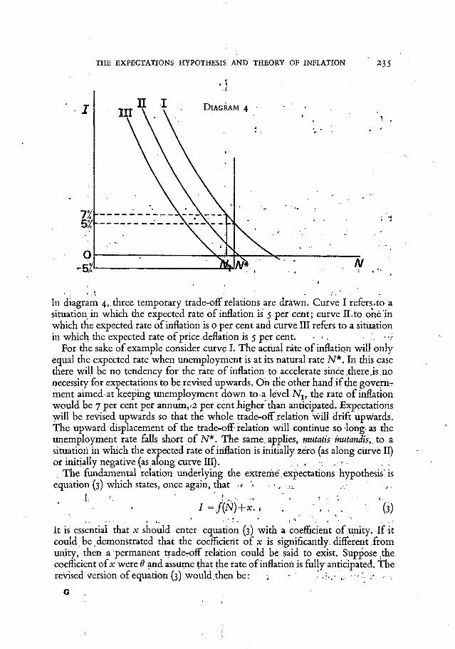
In diagram 4, three temporary trade-off relations are drawn. Curve I refers rto a situation in which the expected rate of inflation is 5 per cent; curve ILto one in which the expected rate of inflation is 0 per cent and curve III refers to a situation in which the expected rate of price, deflation is 5 per cent. • • .

For the sake of example consider curve I . The actual rate of inflation will only equal the expected rate when unemployment is at its natural rate N*. In this case there will be no tendency for the rate o f inflation to accelerate since,there, is no necessity for expectations to be revised upwards. O h the other hand i f the govern­ment aimed at keeping unemployment down to-a level Nlt the rate of inflation would be 7 per cent per annum,.2 per cent higher than anticipated. Expectations will be revised upwards so that the whole trade-off relation will drift upwards. The upward displacement of the trade-off relation will continue so long, as the unemployment rate falls short of N*. The same-applies, mutatis mutandis,, to a situation in which the expected rate of inflation is initially zero (as along curve II) or initially negative (as along curve III). , , •:

The fundamental relation underlying the extreme expectations hypothesis'is equation (3) which states, once again, that .* "?

I=f(N)+x.< •'. " \ • "(3)

It is essential that x should enter equation (3) with a coefficient of unity. I f it could be.demonstrated that the coefficient of x is significantly, different from unity, then a permanent trade-off relation could be said to exist. Suppose the coefficient of x were 8 and assume that the rate of inflation is fully anticipated. The revised version of equation (3) would.then be: -, • . ,?..< ... - •< '•

G

236 . v.:'.: ;. ECONOMIC AND, SOCIAL REVIEW, J . / .

I = / ( N ) + 0 * (8)

Since we have assumed, that the current rate o f inflation is fully anticipated, it follows that I = x. In such a situation, a permanent trade-off relation would emerge, as is indicated by equation (9). , '

(

Equation (9) has important implications for the existence of a stable trade-off relation. For an arbitrarily selected : level of unemployment, any divergence between the actual and expected rate's of inflation wll_qisapjgeaf over time and

the eventual rate of inflation will be ̂ j^L Hence it is not only the natural rate of unemployment that is capable'of sustaining a constant rate of inflation; any positive.rate of unemployment will eventually produce acohstant fate of inflation (which may, of course, be positive or negative inflation). ~

T w o important questions of empirical fact remain to be answered. The first is the^speed of reaction of'the expectations-variable x to recently experienced1 rates of inflation. I f the rate^of inflation were to take'a dramatic turn in an upward direction, how-quickly would the complete upward revision in the expectations variable be accomplished? An answer to this question w i l l depend upon the exact Value'.of' i/'!in"'equation'(6) i I f ^ is near zero,' only the most recently experienced rates o£•inflation' w i l l count and complete 'revision -will be rapid. In contrast, 'if ̂ is' nearer 'unity,' temporally>remote rates'of inflation will be assigned greater importance and the process' of'complete revision will be very slow indeed. This question'has ••wide-ranging .imr)lication's'fo'r economic policy.' I f a government is Oereain-lhaf «cpeCtaidbns'--tok^5a'*long. tMe'tO be revised either upwards or down-wards.wmay'-be'able to behave asif a permanent trade-off between unemployment arid 'iaflatidn-e3dsted'.'«We •r^«urn-it6-tais: qu&tiotf in' Section "4 of this chapter.' ?> The second q'uestion*to •bc'answered'relate's to the precise value "of 6. A value tf£ 6 .wWck'turHSvOut-'to^De" nOt'Sigfiificatitly- different from-unity will constitute strong evidence in favour of the extreme expectations hypothesis.; A value' of 6 which is' not significantly different from zero is evidence;in favour of the extreme version of the permanent trade-off hypothesis.-? '* '•' '\ ;>'>

Such a value (i.e. one which is not significantly different from zero) will imply the existence of widespread "money4illusion'' and many writers on the subject subscribe to the belief that whereas such a phenomenon may be possible in the short-rtui/ib cannot'prevail ihithe lpng !run. H'-must -admit to the'view", writes Gaga^|6],-Uhat;in tne'long run- there is -noWoney illusion and that the coefficient of-price^expectations-variables should* add'up tbtinityi" 'This' a prion conviction seems tO"be:'quite;pef^asive in many of Friedman's writings'; Professor Tobin [8j has subjected this conviction to extensivfe'eriticism.-"trhust Co'nfess-toa strong

sense o£dejd vu," he writes, "The current debate strikes me as the Keynes-classics debate of the 1930's removed thirty years and one time derivative." According to Tobin, "The Phillips curve idea is a reincarnation in dynamic guise of the original Keynesian idea of irrational-'money illusion' in the supply of>labour." The extent of such "money illusion, will be indicated by the magnitude of tlie parameter. • ' • -« •« \ « . J' i. ' i - .< ' • 1

Section 3: The Implications of the Expectations Hypothesis for Optimal Employment . 1. \ ., over Time„ ," • . " ; * '

1 In Section i we examined the procedure by which a goveniment would select the optimum combination of unemployment and'inflation on the assumption that the trade-off relation was stable. iti the long run. This assumption has been questioned by the advocates of the expectations hypothesis' and we examined their views in' Section 2. It will have become apparent by now, however, that a theory which postulates that the trade-off relation is shifting continually (unless unemployment is kept at its "natural" level) will adopt a fundamentally different approach to the problem of an optimal unemployment-inflation mix from that presented in Section 1. In that section, the standard techniques of statical utility maximisation can be validly applied to arrive at an optimal combination of unemployment and inflation which, on the assumption of an unchanging utility function, can'be maintained forever. Such techniques cannot be applied to situations in which the relation is continually shifting due to the selection of particular rates of inflation. The problem of intertemporal optimisation assumes an all-important role and techniques appropriate to the solution of this problem must be called upon. - t

v

The first attempt at framing the problem in terms of intertemporal optimisation was contained in a celebratedvarticle by Edmund Phelps [2] and the analysis presented below is a simplification of his pioneering contribution. Parts 1 to 4 will set out the basic ingredients of Phelps's analysis; parts will state the nature of the problem of intertemporal optimisation in terms of these ingredients; and in part 6 an attempt will be made at solving this problem and at deriving an optimal rule concerning the utility maximising level.of demand.

; \. '•* • \ 1 \

\ ' \".'. v- • Hv ^ 1. The Quasi-Phillips Curve ' N "\ ' T

\ \ ( i Phelps starts off with a concept ^ with whichjwe are by now familiar—the

Phillips curve—but presents it in aNnewj. light. Instead of concentrating upon the relationship between the rate of change of money wage rates and the unem­ployment rate, as Phillips and others have done, he focuses attention on the relationship between the rateof change of prices and-the level of capacity utilisa­tion,)',, the latter being inversely, correlated with'the unemployment rate. In this guise, the strict, expectation's (hypothesis ^becomes.: Y . '

• ••• I -f(y)+x . • (10) -• • • •, . . " • < • ( .

Certain restrictions are imposed upon the variation i n / ( y ) : (i) f'(y)>o which means that the higher the level of capacity utilisation, the greater is the unantici­pated rate of inflation for a-given x. (ii) jf"(y)>o which is the counterpart of a convex Phillips curve where g"(N)>o. (iii) the upper bound of y is y, which is determined by considerations of population and labour supply; moreover, l im/ (y ) = oo. (iv) /x is some minimal level of y ". . . such that output will only

be large enough to permit production of the programmed investment, leaving no employed resources for the production of consumption goods." T h e / ( y ) relationship has another interesting feature; when i" = x,f(y) = 0 and y =. y*, i .e . /(y*) •= o; y* will be recognised as that level of capacity utilisation which will entail a level of unemployment equal to the natural rate of unemployment. These restrictions and properties^ are illustrated in diagram 5 below.

Three hypothetical quasi-Phillips curves are shown in diagram 5; each correspond­ing to a different expected rate of inflation. Curve I corresponds to a positive expected rate of inflation (x 1 >o); curve II corresponds to > a zero expected rate of

inflation (x 2 = 0); and curve III corresponds to a negative expected rate of inflation (x3<o).

The statical utility maximising utilisation ratio is yx when«x'='Xj, y2 when x—x2 and y 3 when x = x 3 . Ingeneral the statical optimal utilisation ratio will be assumed to be a decreasing function of the expected rate of inflation. W e shall assume that the initial anticipated rate of inflation,'x0, is a datum so that we may refer to a single statical optimal utilisation ratio y. *' :

f . 2. The Adaptive Expectations Mechanism v

"V̂ e have, already encountered "this "notion in'Section^ 2 "so that'little further explanation "is necessary, except to rewrite equation (7) in continuous form:

* ~ J t

= a^~x)

= (?({/()•)+x}—x) by equation (10)

V " . . • ' " - G(y)'' ; r ' •] ' .(»)

Hence, the rate of change of the expected rate of.mflation, x, is an increasing function of the utilisation ratio (G'(y)>6) and the.rate of acceleration increases as y increases (G"(y)>o). Moreover, when y = y*, G(y) = 0, i.e. when the expected and actual rates of inflation are equal, there is no tendency for individuals to revise their, expectations in either direction. ( .

3. The Utility Function. • < . •-. Phelps starts out with a utility function which at first sight may appear to have

little relevance to the problem discussed in Section 1. At any point of time, utility is assumed to depend upon two variables: (i) the level of capacity utilisation, y, and (ii) the money rate of interest, i. In symbols, this dependence may be written: . . . -

"U ='4>{i,y)\ ' (12)

The exact nature of the dependence of U on y and i needs to be spelt out in-greater detail before further analysis of the optimisation can take place.

(i) The Relationship between U and y. ' . ' ' " • ' The fundamental dependence of U on y is best illustrated by assuming that the

money rate of interest does not vary and by constructing the following diagram.

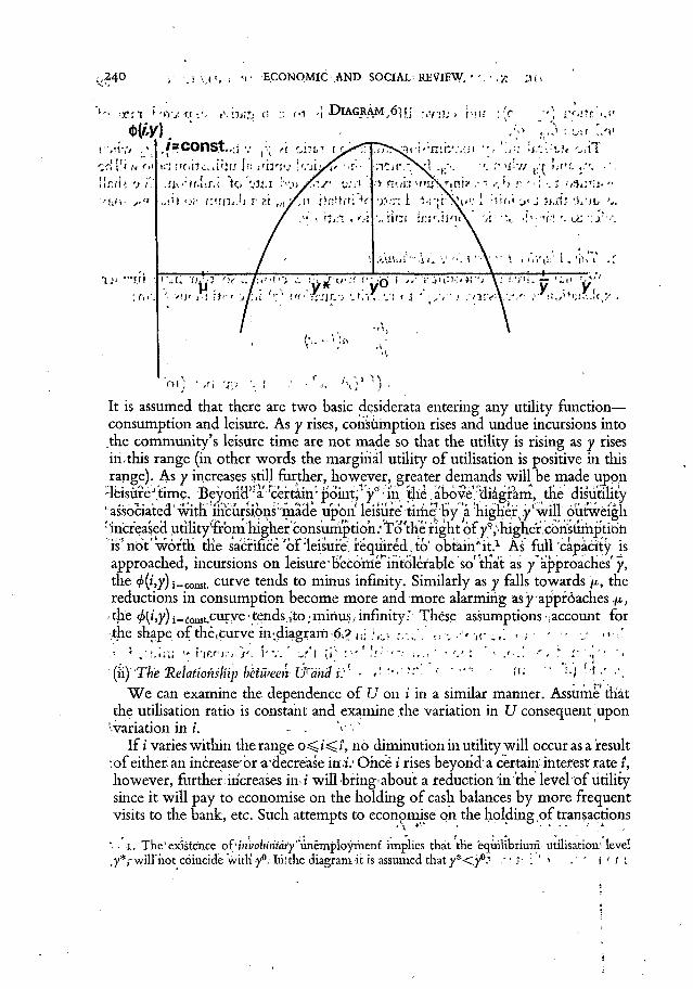
It is assumed that there are two basic desiderata entering any utility function— consumption and leisure. As y rises, consumption rises and undue incursions into the community's leisure time are not made so that the utility is rising as y rises in.this range (in other words the marginal utility of utilisation is positive in this range). As y increases still further, however, greater demands will be made upon

4eisu?eJ.time. Beyond ''afrcertain'-point,*1 y° : in the .above diagram, the disutility 'associated with incursions'made upon leisure time'by a "highef^y'will outweigh : increased utility YrbmMgher consumption.'To'the r̂ of y^higher'consumption is'not'worth the sacrifice 'of "leisure, required,to' obtain''it.1 As full capacity is approached, incursions on leisure'become intolerable so'that as y approaches' y, the 4>{i,y)i^const, curve tends to minus infinity. Similarly as y falls towards '/*, the reductions in consumption become more and more alarming as y approaches

• the 4>(i,y) i-AMutCvirye * tends {to ; minus/ infinity;; These assumptions -account for the shape of the,curve in'diagram:6;? (;i ;,r,- {...,'! v.'^- i - •• / •

'' ;r;,hu " hf,^ir; "ft, |'-'v.' .r'\ {]) : -' ' <-• .... * • ',' i '<..<-..' (ii) "The 'Relationship beiween:Ufti"nd i:' - ' ' " " '«' " '••) -'j •' •'.

W e can examine the dependence of U on i in a similar manner. Assume that the utilisation ratio is constant and examine the variation in U consequent upon

'variation in i. - . • V'••' I f i varies within the range o ^ t ' < i , no diminution in utility will occur as a result

:of either: an increase or adecre'ase in i : Once / rises beyond'a certain interest rate i, however, further, increases i n i will bring'about a reduction in the level of utility since it will pay to economise on the holding of cash balances by more frequent visits to the bank, etc. Such attempts to economise on the holding of transactions

• \ »' • ' * ' . . . . •• •

'• • i . The'existence oiHnvoluntdfy unemployment implies that the equilibrium utilisation' level ,y*,-will'hot coincide with')'0.Iiilthe diagramifcis assumed that y*<y0:- . ' > . ' ' I r i I

^ y , y = c o n s t . -,, , DIAGRAM J,.,

o .vj.»t;l j ,r. 1 . • -'X •••<. \ \ b • :-

•/a.-.'if>i"i'- o\.t .I'-JT,';-'"' >u, iiw I

1-i•":.•.'-''': :.'•!• .titcj.-r «fiT .'. * ' , v \ .(*•(//."< . .'< .»--ix «•.-. rf:-';., 00

balances-will "prod^^ balanc^ ,Hy' :r^u<*ai^ trus leisure timeV:A's'i' approachcS%/:wruch Phelps* calls tfe-bartef points the^'monetary system breaks ''down since the •holding'1 of- 'any'•tianM'tton's *balances'brcdmes prohibitively expensive, li: i*^i, full liquidity is said to exist. • m i J r "

4: The Real and Money Rdtes.of'Iriterestl>\\'<)' > | • "• The money rate of interest, i, is equal to the real rate of interest, r, plus the

expected rate of inflation, x, i.e. 1 = r+x. The^eal rate of interest is assumed to vary directly with the level of capacity' utilisation so that r = r(y). Clearly ,r(y)>o and r'(y)>o; a simplifying but not a crucial assumption is. that r"(y)^o.

l.i, i . . " , . 1 1 'j j (*.»:•>"'"' ', r . . , ' . t ' , ; ( , ' . - ! " U i : ' ' :.>l . i 1 v.'iO <"l <i.'l i

Hence i f i =.r{y)^-x, ,•>( U-=i^{r(y),+;^,y}, ,= ,L7(x,y) i.'/.v •/_/•!<'•' .to:-'i''~--(-i3). " ' • ••'<'..' i «; i i , ,•».«, "Ju'l [' <«,-. ' ' "y l i * " ' ) * J

The expected rate of inflation which is just sufficient to permit full liquidity at t = t, given the level of capacity utilisation, is denoted by x. x satisfies the relation i = r(y)+x for a given y. The'greater is y, the: smaller the expected rate of inflation which is consistent with full liquidity. W e may therefore write x = x(y) where x'(y)<o. O f particular interest in subsequent analysis is thatvalue of x at which there is full'liquidity (i = 1) and equilibrium (y = y*); this value of x is denoted by x(y*).

. ' • '. j \ i \ i ' 1 -»-!.•• q III' i«. T/t j • cj tti j.f , .U'HJ 'i.i'f, j 'j ' . ; u l l 5. The Problem, to beSolved„-n 0 , 4 f-rt .•.-VMD-, ^-'t?rr iv/...v. , ) - O . L U -jrH'

The dynamic problem to be solved consists of the maximisation of social welfare •over time. It involves the discovery, of ah optimal time.path £oT.y'(t)(orx(t)): Social welfare,, W, is the sum.of future utilities' from-1.'= 6 onwards.'This must,be maximised subject'.;to equation ( 1 1 ) , and' therinitial.ucohditioh/that ;;x(6)-;=ix0-. Stated more formally the problem is one of maximising, c >}, r-irjrpn *.-.}' I

2"42 ( ' - E C O N O M I C A N D S O C i A L R E V I E W , 'i

W = foU(x,y)dt > > ; . > o : = (I4)

subject to-^ = G(y) ( n )

j. ' / and x(o) = #„ (15) .<: /

Throughout the remaining analysis we shall assume that the initial expected rate of inflation;-*o> exceeds""£(y*):"We shall see later that x(y*) is the asymptotically optimal expected rate of inflation. 0

6. The Solution of the Problem First of all the simplifying convention is imposed that the level of utility which

corresponds to an expected rate of inflation of x(y*) and a rate of utilisation of y* be set equal to zero, i.e. U(x(y*), y*) = 0. This means that appropriate units of utility-measurement are chosen so as to make>U(.£(y*),y*) equal to.zero. 'u .

. Since £. = G(y) and G, is a monotonically increasing function' of y, we* may write y — G r 1 ^ ) . Substituting into equation (13) the following functional remains to be maximised: ^ ; > , . \ , ; • •.

W= V(x,x)dt.= I V(x,G)dt, ' '(16)

• subject to x(o) = x'0 , .. , .. (15)

This is one of the simplest problems encountered in the calculus of variations and .the solution has been well known to economists since the Ramsey-Keynes problem of optimal savings was posed. The necessary condition for a maximum is that

; ' ^ I / K ( * , ^ - G ^ , G ) = O " ' ' :MT)

. • , G ; = VG{x,G) where F g(JC,G) = ^ .

This optimal condition must be met at all points in time from t = o onwards. The value of G which satisfies equation (17) at a point in time is the optimal rate

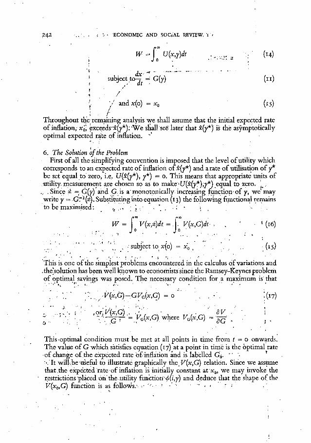
-of change of the expected rate of inflation and is labelled G<j. " - * • >,Tt will.be useful to illustrate graphically the. F (x ,G) relation. Since we assume that.the expected rate of inflation is initially constant at x0, we may invoke the restrictions placed on the.utility function'<f>(i,y) and deduce that.the shape of the V(x0,G) function is as follows.' - -• . • < • 1 . '

V(x{y»)rG)

Vfx^G)

Suppose now-that the expected rate of inflation fell to xx: the level of utility is approached'for all G,-i.e. the curve will have shifted upwards. This upward drift will continue until the curve reaches its limiting position which coincides with the curve V[x(y*),G) which, due to our felicitous choice of units, passes through the origin. The curve will cease to drift once x = x(y*) since full liquidity will have been reached and no increase in utility will be achieved by a further fall in the expected rate of inflation. W e ate now in a position to interpret the optimality rule set out in (17) in terms of diagram 9 below. ' • « ' » - . -

1 • . . . .

At a point in time, the optimal value of G (and hence of y) is found by drawing a line AO through thejorigin in such a way that it is tangential to the V(x0,G) curve. Denote the point of tangency-by.the symbol At -A, the slope of the

V(x0,G). V(x0,G) function viz. VG(x0)G), is equal to the slope of the tangent, Q— This optimality condition is thus satisfied at point </». It follows that the optimal rate of decrease of the expected rate of inflation is G 0 , which is found by drawing a vertical line from t/i to the'G(y) axis. Noting* that the optimal rule at time t = 0 requires a negative G(y), we deduce that initially a government must follow a policy' of underutilisation so as to drive down the expected rate of inflation.

?244 '<•:.• -I'.-U 'i-> ECONOMIC'AND' SOCIAL REVIEW"'("•• -iXti a"*.

<> „ , „ , ( • DIAGRAM 9

Having located the/initially optimal G , we must examine how the optimal value of G changes, if at all, with the passage of time. As we said previously, a decline in the expected fate (of inflation will shift the V(x,G) curve bodily upwards. The conthiuing upward drift of this curve to its limiting position V(x(y*),G) implies that as time passes, the point of tangency will be drifting in a north-easterly

. direction and will ultimately cbincide with the origin. The asymptotically optimal - expected- rateof inflation, is &{y*), and once, this expected rate,of inflation is established;, it will .remain .optimal ;forever. (since, as ̂ - 7 ^ 0 0 : , G ==.0 becomes i';the

r .optimal rate o f change of the expected rate of inflation). ;\) ••• ; , - y -,p ! ' i v v- 'F M -.-•>« i-« "-V-.7 - . V ' . h <<i "" ' i»;v •• , .1 '.5:'•*{-> •

t Summary,\r> ,. „ • j ; , 7 , . . „ • ; . , , ,.; , - ; { : „ ...... . , ' . , .-„.<'

'••We have seen how the optimal rule givendn equation (17) states that7, when the initial expected rate of inflationexceed.s,^()'*);'the government should undertake a policy of underutilisation. Following such a policy, the government would have to "push the -unemployment' rate above its natural level, even though'(as we have

^assumed) the'statically -optimal 'unemployment"rate may be below the natural ' rateP This is •illustrated' in"*'the' moire '.familiarj Phillips "curve diagram which .'fo'UoWS. _ , ; . . ,• T - • X »

The natural rate of unemployment is'N* ahd'the'unemploymen't rate which is .statistically optimal, ion the ̂ assumption that the. expected rate of inflation is<-%

•asiT^.-The 'optimal rule states.that unehroloyment shomd -be-pusta .order,to'lower the expected.rate of inflation-and gradually, shift the temporary .trade-off relation from<position-1 to-position.II: Moreover,";once the process of shifting the.tfade-roff relation downwards has'beenrset/ih motion,- demand- and

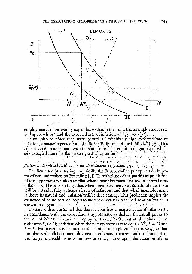
employment can be steadily expanded so that in the limit, the unemployment rate will approach N* and the expected rate of inflation will fall to x(y*). ,

It will, also be noted that; starting with'an excessively high'expected'rate of inflation, a unique expected irate of inflation1 iis^optimal iti the ,limit.viz.'<^(y*).f,This conclusion 'does not square with the static 'approach' set out in'diagra'm 4 in which any expected rate of inflation can yield'ah 6pdmum!.r|j':." 1 ' ' ' •' 3 V ' 4 !

• / • , 1 . • . ' u 1 - * 4{i , -A'-1 r . <-SA," ••• i« .,(:'-j-r • Section 4: Empirical-Evidence on the Expectations,Hypothesis c<\ K , u , , j •»• >' • t-«

The first attempt at testing1 empirically the Friedman-Phelps expectation hypo­thesis was undertaken b'y/Brechling •. [9].~, He makes use of the particular; prediction of this hypothesis which states that when unemployment is'below its natural rate, inflation will be accelerating;: that when unemployment;is at its natural rate,.there will be a steady, fully anticipated rate ofinflation';;and that when unemployment is above its natural rate, inflation'wilLbe decelerating. This (prediction implies the existence of some sort of loop'around'the.short^run-trade-bffxelation which'is shown in diagram 11. > •< •': , , . « ••, . MCV .,.<•• I .>:• '

T o start with it is assumed that there is a positive anticipated rate'of inflation / j . •In accordance with .the" expectations hypothesis,-.we deduce that at all points to the left of AT*,1 the natural unemployment rate, , i>0; that at all points to the right o£N*, i<0; and'that when the unemployment rate equals N*, I — O and I = Iv.Moreoverit is assumed that the initial-unemployment rate is N,,', so that the observed inflation-unemployment combination corresponds to. point A-in the diagram. Brechling now imposes arbitrary JimitS'Upon theivariatori-ofnhe

DIAGRAM II

unemployment rate. He makes the simplifying but,expendable assumption that , the unemployment rate varies smoothly between a lower limit Na and an upper .limit Nb (which for the sake of convenience coincides with the initial unemploy­ment rate). If N* falls within thetinterval (Na, Nb), then the expectations hypo­thesis will predict that clockwise loops will occur around the f(N) relation. To illustrate how this phenomenon arises, we have assumed that the unemployment rate has just risen to its upper limit Nb and that from now on the government will undertake'over a period of time such policies as will bring the unemployment rate down to its lower limit Na. Since Nj, ;>N*,'there will be a tendency for the rate of'inflation to fall as N falls from Nb to N*; this tendency will be arrested when N reaches N*; and it will be reversed (i.e. inflation will accelerate) as N ;rises beyond N*. The nearer the unemployment rate is pushed towards JV 0

!, the faster the rate of inflation" accelerates. I f we make the additional assumption that once ;Na is treached the government will undertake the appropriate measures needed to drive AT steadily upwards towards A^, the opposite process will occur: the.rate of inflation will tend to decelerate. When point D is reached, the rate of inflation will have reached its maximum and will start falling as the unemploy­ment rate is raised towards Nb. It is clearly an implication of the expectations •hypothesis that, if such smooth variations in unemployment were actually to occur, then clockwise loops of the sort described would develop even in the short run, provided1, of course, that N* is less than Nb and greater than Na (an alternative test being appropriate when this proviso .cannot be met).

As a test for this hypothesis using American data, Brechling assumes that Na = 3 per cent, that Nb = 9-percent and that there is a smooth cycle between these two limits. Using his own trade-off equation to predict the variation in the rate of inflation which would be produced by the smooth cycle of unemployment between its two limits, he discovered that the loops so generated rotated in an anticlockwise direction, which is contrary to the prediction of the expectation hypothesis. As further support for his contention, Brechling points to numerous econometric studies which discovered that when the rate of change of unemploy­ment was included as an additional explanatory variable in regression equations, it in general entered with a negative coefficient. That is, it was generally found that when unemployment is falling, the rate of inflation is higher than when it is rising. This phenomenon produces. anticlockwise loops and lends support to Brechling's tentative refutation of the expectations hypothesis.

Following upon the work of Brechling, a more searching econometric study was undertaken by Professor Solow [7]. Although his data referred to both British and American-experience, the author himself placed greater trust,'for a variety of reasons, in the results for the-American economy and these will be subjected to closer scrutiny in this section, > . • .

The fundamental relationship which he attempts to test directly is an equation similar to equation (8) of Section 2; in that equation all other real variables apart from the unemployment rate were assumed, for expositional purposes, to exert an insignificant influence upon the rate 'of inflation. Such an approach is highly suspect, however, when one attempts to construct a realistic econometric model of the process of price inflation; many more real variables will have to be included before the model can be considered as even a plausible approximation to reality. This may be overcome by rewriting equation (8) in the following way:

I = / ( Z ) + * . . . (10) ' - - ' . - • ' >. -

where Z is a vector of real variables: The components of the Z vector are somewhat different in Solow's study from those included in other studies of the_ trade-off relation. < - > . .

For a measure of aggregate demand, Solow prefers to use a measure of capacity utilisation rather than,the overall.unemployment rate; moreover, his measure of capacity utilisation is highly non-linear and is a transformation of,the capacity utilisation index published by the Wharton School at ,the .University of Pennsylvania. , , . ' • - > . , . r .

Solow also attempts to separate, out the distinct effects of variations in the money wage rate from variations in labour productivity: since the rate of change of unit labour cost, ulc, is equal to the 'rate of change of money wage rates, w] plus the reciprocal of the rate of change of output per man,'r, a theory which states that an increase in unit labour cost arising from an increase in money wage rates will have the same effect on prices as an increase in unit labour costs arising from a fall in output per man will not require any breakdown of the unit labour

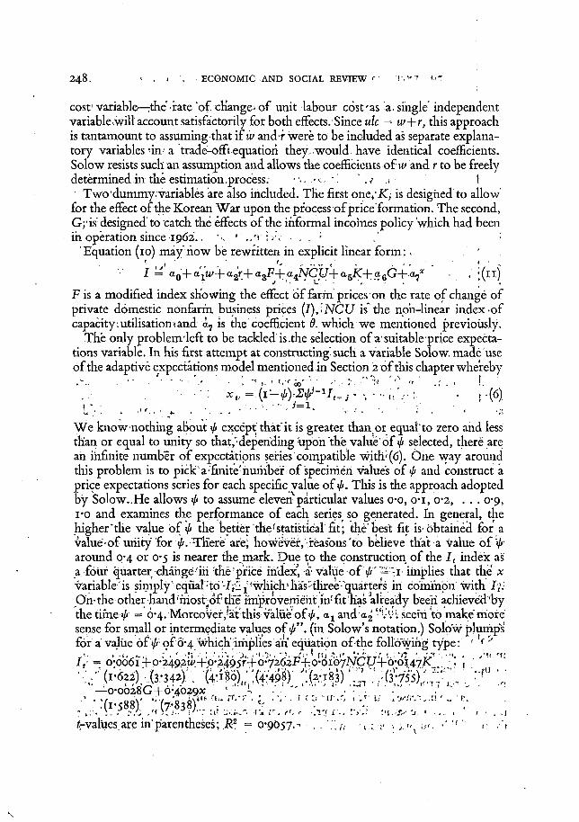
cost variable—the'irate of ch'ange< of unit, labour cost'as a, single independent variable .will account satisfactorily for both effects. Since ulc = u>+r, this approach is tantamount to assuming that i f u> and'f were to be included as separate explana­tory variables 'in* a trade-off (equation they, would have identical coefficients. Solow resists such an assumption and allows the coefficients of w and r to be freely determined.in the estimation.process: ' I " Two'dummy, variables are also included. The first one/K, is designed to allow for the effect of the Korean War upon the process of price formation. The second, G;is' designed'to catch the effects of the informal incomes policy which had been in operation since 1962.., "•'.,'«•; . , - .' :

Equation (10) may how be rewritten in explicit linear form: . ' ' ' ,j< ' f , - ' '- • - <• < - - - • ' - ; ' -I = a 0 + a x W + a 2 r + a 3 P + a 4 N C U + a 5 K + a 6 G + a 7

; , r , *(ll)

F is a modified index showing the effect of farm prices on the rate of change of private domestic nonfarm business prices (l),-iNCU is the non-linear index of capacity L utilisation! and a 7 is the coefficient 6. which we mentioned previously.

The only problenrleft to be tackled'is .the selection of a'suitable price expecta­tions variable. In his first attempt at constructing such a variable Solow. made use of the adaptive expectations model mentioned in Section 2 of this chapter whereby

V* ' ^ - ( i - ' ^ V - 1 / , - ^ : : - u ' A ""• r ( 6 ) . . . . • • <••• • • ,

W e knownothing about </> except that" it is greater than or equal to zero and less than or equal to unity so that,* depending upon the value of ^ selected, there are an infinite number of expectations series compatible with ;(6). One way around this problem is to pick'a ;finite'number of "specimen value's of <f> and construct a price expectations series for each specific value of 0. This is the approach adopted by Solow..He allows ^ to assume eleven particular values o-o, o-i, 0-2, . . . 0*9, i*o and examines the performance of each series so generated. In general, the higher'the value of </< the better the'statistical fit; the best fit is-obtained for a value-of unity for ty. -There are; however,'reasons'to believe that-a value of around 0*4 or 0*5 is nearer the,mark. Due to the construction of the I , index as a four quarter change-ih the'price index, -avalue-of ="i implies that the x variable is simply'equal 'to -Iju{"which'has-three''quarters in common with T' t\ ;

On-the other hand mostof the* improvement in : fit -has already been achieved'by the time >p = 6-4. MoreoVerJat this valiie'of </>, a.1 and <x2' seem to make more sense for small or intermediate values of <p". (in Solow's notation.) Solow plumps for a value of <l> of 6*4 which' implies an equation o f the following type: ' r ' '

I , - 6-6b6i^p-2492w+p'24^ 'f . ' ' '' (1-622).( 3-342) :. ( i - i B o ) , ; ^ ^ ) ' \?,.;4;iss);Z':\:.'.

—o-oo28G+o-4029x . . . • .-(1.588)' • ! < ' M ; f - v M ' . . , - .

(-values are in'parentheses1; R2 = 0.9057.^ /,• r , y„ y<. >' " " f f

It is clear that the coefficient ^•(a, in equation (n) ) is significantly different from unity. Moreover 9 remains significantly different from unity for A// 1 values'of tji selected for the x series. I f this is so1 then it constitutes strong evidence in favour of the notion that a permanent trade-off'surface does, in fact exist even though expectations of inflation do play an important role in'determining the actual rate of inflation. Furthermore, i f any confidence can be placed, in a value of <fi of. around 0*4 it implies that the revision of expectations takes a long time to occur. In conclusion' Solow states: "Whatever' may be true of. Latin-American-size inflations or even smaller, perfectly steady inflations, tinder conditions that really matter—irregular price increases with an order of magnitude of a few percent a year—there is a trade-off between the speed of price increase and the real state of the economy. It is less favorable in the long run than it is at first. It may not be 'permanent'; but it is long enough for me."

The empirical research of Brechling and Solow outlined above would appear to point to the conclusion that a permanent trade-off between inflation and unemployment (or some other measure of aggregate demand) does in fact exist. The work of Brechling draws out certain qualitative implications of the expecta­tions hypothesis which, on the basis of the evidence cited, fail to be met in reality. Solow's approach is more direct in that he attempts to estimate the values of the parameters d and 0. He deduces that ip is probably around 0*4, which implies that complete adjustment to a new higher rate of inflation will probably be quite prolonged. More important still, he estimates that the value of 6 is significantly different from unity which constitutes a refutation of the strict expectations hypothesis. Further research clearly needs to be carried out in this field and the last word has by no means been said so far in the debate. Anticipating many of the future studies on the subject, Professor Tobin [8] predicts that " . . . sooner or later an econometric study will surely enough produce the magic number one for the price coefficient. . .". Not a very hopeful note to end a paper with.

Trinity College, Dublin.

REFERENCES

[1] M. Friedman, "The Role of Monetary Policy", American Economic Review, March 1968. [2] E . S. Phelps, "Phillips Curves, Expectations of Inflation and Optimal Unemployment Over

Time", Economica, August 1967. [2a] E . S . Phelps "Money-Wage Dynamics and Labour-Market Equilibrium",/o«r«a/ of Political

Economy, July-August, 1968. [3] R. G. Lipsey, "The Relation between Unemployment and the Rate of Change of Money

"Wage Rates in the United Kingdom, 1862-1957; A Further Analysis." Economica, February i960.

[3a] R. G. Lipsey, "Structural and Demand Deficient Unemployment Reconsidered", in R. M. Ross (ed.), Employment Policy and the Labour Market, University of California Press, 1965.

[4] A. W . Phillips, "The Relation between Unemployment and the Rate of Change of Money (Wage Rates in the United Kingdom, 1861-1957", Economica, November 1958. • „ •» •

[5] P. Cagan; "The Monetary Dynamics of Hyperinflation", in M. Friedman (ed.) Studies in the Quantity Theory of Money, University of Chicago Press, 1956.

[6] P. Cagan, "Recent Statistical Studies'on Wage-Push Inflation", Symposium on Inflation, New York University, 1968. (rnimeographed paper). ' '

[7] R. M. Solow, Price Expectations and the Behaviour of the Price Level, Manchester University Press, 1969. r, .. , .

[8] J . Tobin,, "Comment on Professor Cagan's Paper!', Symposium on Inflation, New York University, 1968. (mimeographed paper).

[9] F. Brechling, "The Trade-Off between Inflation and Unemployment", Journal of Political Economy, July-August, 1968. . ' .