
The Evolutionary Design of Digital VLSI Hardware
183
a : :77 !.Ihh, N ift -7 9"17'All -Iftlwiaga-v- N) r - - — - — - L - — - . . F 4z The Evolutionary Design of Digital VLSI Hardware Robert Thomson A thesis submitted for the degree of Doctor of Philosophy. The University of Edinburgh. October 2005
Transcript of The Evolutionary Design of Digital VLSI Hardware

a
: :77 !.Ihh, Nift-79"17'All
-Iftlwiaga-v- N)
r - -
— - — - L - — -
. .
F 4z
The Evolutionary Design of Digital VLSI Hardware
Robert Thomson
A thesis submitted for the degree of Doctor of Philosophy. The University of Edinburgh.
October 2005

Abstract
Evolutionary Algorithms (EAs) are a class of powerful stochastic search techniques, which
were inspired by natural evolution. They work by iteratively improving a population of solu-
tions, according to one or more objective functions. Evolutionary algorithms are capable of
producing near-optimal solutions to highly complex search problems;
In this thesis, multi-objective evolutionary algorithms are applied to the design of efficient
digital ASIC core designs. Specifically, the thesis addresses the evolutionary synthesis of mul-
tiplierless linear filters, multiplierless linear transforms, and polynomial transform designs. The
designs are constructed from high-level arithmetic components such as adders and subtracters,
according to a user-supplied behavioural specification. The designs are evaluated according to
three different objectives: functionality, low area requirements, and low longest-path delay. In
order to evaluate these objectives, accurate hardware models are developed.
Evolutionary algorithms are often applied to scheduling problems. This thesis investigates
the possibility of performing scheduling and allocation in parallel with circuit evolution. Two
possibilities are considered: scheduling for sequential operation and pipeline scheduling.
The choice of solution representation and evolutionary operators can have an enormous im-
pact on the performance of an evolutionary algorithm. In this thesis, solutions are represented
with graphs. Graphs are found to be a powerful and intuitive representation for circuit designs,
although the complexity of the evolutionary operators tends to be higher than with other encod-
ings. Various graph evolutionary operators are developed, including a novel non-destructive
graph crossover operator.
This thesis also proposes a class of local search operators. These operators can significantly
improve the performance of an EA. The improvement is achieved in two ways: by reducing
the computational cost of evaluating a design, and by automatically finding optimal settings
for some of the design parameters. These local search operators are initially applied to linear
designs, and are later adapted for devices with polynomial responses.

Declaration of originality
I hereby declare that the research recorded in this thesis and the thesis itself was composed and
originated entirely by myself in the School of Engineering and Electronics at The University of
Edinburgh.
Figure 2.11 is based upon a figure in [1].
Robert Thomson
IIII

Acknowledgements
Thanks to my parents, for their constant support.
Thanks to Ben Hounsell for his help early in my research.
Thanks to Tughrul Arsian and Alister Hamilton for supervising this PhD.
Thanks to John Hannah, for encouraging me to write up quickly.
lv

Contents
Declaration of originality iii Acknowledgements ................................iv Contents ....................................... V
List of figures ................................... IX
List of tables ................................... XII
Acronyms and abbreviations . . . . . . . . . . . . . . . . . . . . . . . . . . . xiii Nomenclature ................................... xv
1 Introduction 1
1.1 Motivation ......................................1
1.2 Contribution ....................................2
1.3 Overview .....................................2
1.4 Thesis contents ..................................3
2 Hardware modelling and synthesis 7
2.1 Introduction .................................... 7
2.2 Digital signal processing ............................. 7 2.2.1 Linear filtering ................................ 7
2.2.2 Linear Transforms ............................ 10
2.2.3 Nonlinear filtering ............................ 12
2.3 Filter implementation ............................... 13
2.3.1 Hardware implementation of linear components ............. 13 2.3.2 Carry-save arithmetic ........................... 14
2.3.3 Multipliers and multiplication blocks .................... 14 2.3.4 Linear transforms .............................. 19
2.3.5 Existing linear filter design systems ................... 21
2.3.6 Implementation of Volterra filters .................... 21
2.4 Hardware properties and modelling ........................ 22
2.4.1 Pre-placement modelling .......................... 23
2.4.2 Wire-load modelling ........................... 23
2.4.3 Longest path delay ............................ 24
2.4.4 Power ..................................... 27
2.4.5 Silicon area ................................ 29
2.4.6 Other metrics ............................... 29
2.5 Summary ...................................... 30
3 Evolutionary algorithms and stochastic search techniques 31 3.1 Introduction ....................................31 3.2- Evolutionary algorithms .............................31
3.2.1 Operation of an evolutionary algorithm .................32 3.2.2 Fitness landscapes ............................34 3.2.3 A taxonomy of evolutionary algorithms ................. 35
V

Contents
3.2.4 Other stochastic search techniques .................... 36 3.2.5 Hybrid search techniques ......................... 37
3.3 Multiobjective evolutionary algorithms ....................... 37 3.3.1 Multiobjective problem solving ..................... 37 3.3.2 Non-Pareto ranking methods ....................... 39 3.3.3 Pareto ranking methods .......................... 40 3.3.4 Population diversity ........................... 41 3.3.5 Multiobjective elitism ......................... 42
4 Evolutionary algorithms and electronics ..................... 42 3.4.1 The evolution of electronic designs .................... 42 3.4.2 Assessing functionality ........................... 46 3.4.3 The genotypic representation of digital circuits ............. 47
3.5 Summary ..................................... 51
4 Evolutionary algorithms for FIR filter synthesis 53 4.1 Introduction ....................................53 4.2 Problem description ................................54 4.3 System description ................................56
4.3.1 Objective calculation ...........................56 4.3.2 The chromosome .............................57 4.3.3 Initialisation ............................... 59 4.3.4 Evolutionary operators ..........................60 4.3.5 Ranking and selection ..........................61 4.3.6 Elitism ..................................62 4.3.7 The evolutionary algorithm ........................63 4.3.8 Circuit synthesis .............................63
4.4 Experiments and results ...............................65 4.41 Evolution of filters .............................65 4.4.2 Crossover rate ..............................66 4.4.3 Comparison with other systems ......................68
4.5 Summary ......................................72
5 The evolution of sequential circuits 73 5.1 Introduction .................................... 73 5.2 Multistate sequential circuits ........................... 73 5.3 2-state hardware .................................. 74 5.4 Modifications to the EA .............................. 75 5.5 Results ....................................... 77 5.6 A multistate accumulation block .......................... 81 5.7 Operation over many cycles ............................ 81 5.8 Application to other problems .......................... 82 5.9 Summary ..................................... 82
6 The evolution of multiplierless linear circuits
85 6.1 Introduction ................ 85 6.2 Problem statement ............ 85 6.3 The evolution of linear transforms . 86
vi

Contents
6.3.1 The chromosome 86
6.3.2 Initial population .............................8 7
6.3.3 Evolutionary operators ..........................87 6.3.4 Fixed-point and integer operation ....................88
6.3.5 Assessment of functionality .......................89 6.3.6 Hardware modelling ............................89
6.3.7 Ranking and selection ..........................90
6.4 Experiments .................................... 91
6.4.1 Test problems ................................91
6.4.2 Solution functionality ..........................92
6.4.3 Solution quality and diversity ......................93 6.4.4 Hardware implementation styles .....................94
6.4.5 Fixed-point values ............................95
6.4.6 Hardware modelling ...........................96 6.4.7 Comparison with other design techniques ................96
6.5 Summary ..................................... 97
7 Local searches and the evolution of linear circuits 99
7.1 Introduction .................................... 99
7.2 Design modelling .................................99
7.3 Characterising a design ..............................103
7.4 Searching evolutionary operators .......................... 103
7.5 Experiments and results .............................. 105
7.6 Summary ..................................... 108
8 Local searches and the evolution of nonlinear circuits 111
8.1 Introduction ..................................... 111
8.2 Filter specification ................................ 1 11
8.3 The EA ....................................... 112
8.3.1 The chromosome ............................. 112
8.3.2 Initial population ............................. 113
8.3.3 Local searches .............................. 113
8.3.4 Functional evaluation ........................... 114
8.3.5 Hardware modelling ............................ 115
8.3.6 Evolutionary operators .......................... 116
8.4 Experiments and results ................................ 117
8.4.1 An example problem - the sine function ................ 117
8.4.2 Application to larger problems ...................... 119
8.4.3 Scalability of the current system ...................... 120
8.4.4 Effectiveness of the local searches .................... 122
8.5 Summary ..................................... 124
9 Enhancements 125
9.1 Introduction ....................................1 25
9.2 System overview .................................125
9.2.1 Representation ..............................125
9.2.2 Evolutionary operators .......................... 126
vu

- Contents
9.2.3 Populations and selection .........................126 9.3 Pipeline scheduling ................................127 9.4 Improved delay modelling ............................128 9.5 Experimental methodology ............................130 9.6 Initial experiments .................................132 9.7 A reduced parameter space ............................134
9.7.1 Changes to the chromosome .......................134 9.7.2 Experiments ................................135 9.7.3 Analysis .................................137
9.8 Neighbour crossover ...............................138 9.8.1 The neighbour crossover algorithm ...................138 9.8.2 Experiments ...............................140
9.9 Summary .....................................143
10 Conclusions 145 10.1 Introduction ....................................145 10.2 Review of thesis contents .............................145 10.3 Specific findings ..................................147 10.4 Directions for further research ..........................149 10.5 Summary .....................................150
A Publications 153 A.1 Refereed publications .............. 153 A.2 Patent application ................ 153
B Transform matrices and filter responses 155
C Nonlinear problem specifications 157
References 159
viii

List of figures
2.1 A direct form FIR filter 8
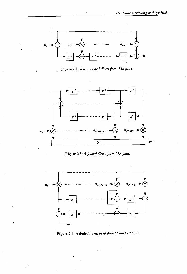
2.2 A transposed direct form FIR filter ......................... 9
2.3 A folded direct form FIR filter . . . . . . . . . . . . . . . . . . . . . . . . . . . 9
2.4 A folded transposed direct form FIR filter . . . . . . . . . . . . . . . . . . . . . 9
2.5 A discrete wavelet transform (DWT) with 3 levels of decomposition . . . . . . . 12
2.6 Three implementations of A + 8B. Clockwise from top left: bit-serial, 4-bit
digit-serial, and bit-parallel . . . . . . . . . . . . . . . . . . . . . . . . . . . . . 13
2.7 The summation of three values using carry-save arithmetic . . . . . . . . . . . . 15
2.8 A suboptimal CSD multiplier: multiplication by 45................ 17
2.9 Common sub-expression elimination . . . . . . . . . . . . . . . . . . . . . . . 18
2.10 Designing linear transform hardware using the iterative matching algorithm. . 20
2.11 The decomposition of a Volterra filter proposed by Panicker and Mathews[1, 2] 22
2.12 Two wire load models . . . . . . . . . . . . . . . . . . . . . . . . . . . . . . . 23
2.13 A model of a balanced tree wiring structure with N = 3 branches of equal length. 24
2.14 Elmore delay models for (a) a chain of RC delays and (b) a tree of RC delays with a single driver . . . . . . . . . . . . . . . . . . . . . . . . . . . . . . . . . 25
2.15 Three models of the delay in a 4-bit negator: per connection, per bit and per group of bits .................................... 26
2.16 Two four-bit ripple adders, with a combined delay of 5 full adders, while a single adder has a delay of 4 full adders . . . . . . . . . . . . . . . . . . . . . . 26
2.17 Dynamic power consumption in a CMOS inverter . . . . . . . . . . . . . . . . . 27
3.1 The operation of an EA. An initial population is created and then iteratively replaced. . . . . . . . . . . . . . . . . . . . . . . . . . . . . . . . . . . . . . . 32
3.2 Crossover and mutation as applied to a binary chromosome . . . . . . . . . . . 33 3.3 Point a dominates point b, while both a and b are dominated by some of the
points on the Pareto surface . . . . . . . . . . . . . ... . . . . . . . . . . . . . 38
3.4 Selection pressure towards optimal solutions (solid arrows) and a diverse solu- tion set (dashed arrows).............................. 38
3.5 A concave Pareto surface with Pareto points A, B, and C, where point B is in a concavity...................................... 39
3.6 The ranks assigned to a population by the non-dominated sorting algorithm. 40
4.1 An example filter specification - the response of the filter must be in the shaded area at all frequencies ...... ... ... ... ...............55
4.2 The multiplication block and the accumulation block in a transposed direct form FIR filter................................... 55
4.3 Calculation of the functionality objective, which is defined as the largest devi- ation from the specification (in this example at f = 0.125)...........56
4.4 Conversion from the genotype to the phenotype . . . . . . . . . . . . . . . . . . 58
4.5 A breakdown of the contents of the chromosome . . . . . . . . . . . . . . . . . 59
ix
List of figures
4.6 The heuristic mutation operators . . . . . . . . . . . . . . . . . . . . . . . . . . 60 4.7 Selection: (a) by rank, and (b) by both rank and functionality . . . . . . . . . . . 62 4.8 An example filter netlist . . . . . . . . . . . . . . . . . . . . . . . . . . . . . . 63 4.9 An evolved filter . . . . . . . . . . . . . . . ... . . . . . . . . . . . . . . . . . 64
4.10 Filter specifications . . . . . . . . . . . . . . . . . . . . . . . . . . . . . . . . . 64 4.11 The number of populations containing a correct solution, by generation. . . . . 65 4.12 Area and delay results for low-pass (left) and high-pass filters (right) . . . . . . 66 4.13 Experiments with different levels of crossover, for the 40dB low-pass (left) and 17 high-pass (right) problems . . . . . . . . . . . . . . . . . . . . . . . . . . . . . 67 4.14 Comparison of component counts with the modelled areas . . . . . . . . . . . . 69
5.1 2-state and n-state state machines . . . . . ... . . . . . . . . . . . . . . . . . . 74 5.2 A 21-times multiplier using two additions, performed using one adder, two
MUXs and one register ................................74 53 How the position of an operation within the chromosome is used to encode
scheduling and binding information. ........................75 5.4 Correct results for the test problems . . . . . . . . . . . . . . . . . . . . . . . . 77 5.5 Critical paths. The last adder (shown in grey) is always part of the accumulation
block .........................................78 5.6 Comparison of sequential and equivalent combinatorial areas for evolved mul-
tiplication blocks ..................................79 5.7 Comparison of sequential and equivalent combinatorial areas for evolved filters 79 5.8 A 2-state accumulation block ..... ... ....................81
6.1 A chromosome and the corresponding circuit design ................86 6.2 The functional fitness of the best DHT design, for 20 runs . . . . . . . . . . . . 92 6.3 Properties of the evolved circuits for the test pr oblems . . . . . . . . . . . . . . 93 6.4 Minimum area and minimum delay circuits for computing f = a + b + c + d
and g = b + c + d . . . . . . . . . . . . . . . . . . . . . . . . . . . . . . . . . 94 6.5 Properties of 4-point DCT designs evolved with 3 different hardware models. 94 6.6 Functional fitness in integer mode (upper lines) and fixed-point mode (lower
lines) . . . . . . . . . . . . . . . . . . . . . . . . . . . . . . . . . . . . . . . . 95 6.7 A comparison of the hardware models with Synopsys Design Compiler . . . . . 96
7.1 A model of how a single connection (labelled 'X') relates to the inputs and outputs of a linear system . . . . . . . . . . . . . . . . . . . . . . . . . . . . . 100
7.2 The effect of inserting a shift and negation into a connection . . . . . . . . . . . 102 7.3 A model of how the 'insert node' operation changes a design . . . . . . . . . . . 105 7.4 The functional error of the most functional DHT design, by generation . . . . . 106 7.5 Comparison of result delay and area between the original EA system and the
searching EA system . . . . . . . . . . . . . . . . . . . . . . . . . . . . . . . . 107
8.1 A model of a nonlinear system, where one connection has been selected for modification ....................................114
8.2 The properties of evolved sine circuits . . . . . . . . . . . . . . . . . . . . . . . 118 8.3 The response of an evolved sine circuit, and the error when compared to an
ideal sine . . . . . . . . . . . . . . . . . . . . . . . . . . . . . . . . . . . . . . 118 8.4 The properties of the functional solutions to the test problems . . . . . . . . . . 120
x

List of figures
8.5 Circuit properties for the non-searching and searching EAs . . . . . . . . . . . . 123
9.1 Two ways of repairing an invalid schedule . . . . . . . . . . . . . . . . . . . . . 128 9.2 RC delays according to fanout . . . . . . . . . . . . . . . . . . . . . . . . . . . 129 9.3 Calculation of attainment surfaces: the four non-dominated surfaces in (a) are
converted to four attainment surfaces in (b)....................130 9.4 Solution properties according to pipeline depth . . . . . . . . . . . . . . . . . . 132 9.5 The hardware models compared with Design Compiler . . . . . . . . . . . . . . 133 9.6 Performance comparisons between the original EA (light grey) and the reduced-
parameter EA (dark grey) . . . . . . . . . . . . . . . . . . . . . . . . . . . . . 136 9.7 Attainment surfaces for the original and reduced-parameter EAs . . . . . . . . . 136 9.8 The relationship between normalised and un-normalised responses . . . . . . . . 137 9.9 One step of the neighbour crossover region growing process . . . . . . . . . . . 138 9.10 Neighbour crossover (light grey) compared to other techniques (dark grey). . . 141 9.11 5% and 10% attainment surfaces, with various crossover operators . . . . . . . . 142
lug

List of tables
4.1 Component costs . 57 4.2 EA settings . . . . . . . . . . . . . . . . . . . . . . . . . . . . . . . . . . . . . 65 4.3 EA performance................................. 66 4.4 Comparison of component counts for evolved and conventional filters . . . . . . 68 4.5 Comparison of the number of adders on the longest path, for evolved and con-
ventional filters . . . . . . . . . . . . . . . . . . . . . . . . . . . . . . . . . . . 70 4.6 A filter specification from Suckley [3].......................70 4.7 Comparison with results from Redmill et aL [4]..................71
5.1 Component properties . . . . . . . . . . . . . . . ... . . . . . . . . . . . . . . 77 5.2 Component counts for three different filter implementation techniques . . . . . . 80 5.3 Components required for an n-th order accumulation block .. . . . . . . . . . . 80
6.1 Bit-serial component properties . . . . . . . . . . . . . . . . . . . . . . . . . . 90 6.2 Functionality results from the test problems . . . . . . . . . . . . . . . . . . . . 92 6.3 Adder counts for evolved and non-evolved solutions to the test problems. . 97
7.1 Functionality results from the test problems . . . . . . . . . . . . . . . . . . . . 105 7.2 Lowest-area and lowest-delay design properties for the original and searching
EAs . . . . . . . . . . . . . . . . . . . . . . . . . . . . . . . . . . . . . . . . . 106 7.3 Adder counts for evolved and non-evolved solutions to the test problems. . 107 7.4 Time taken for each experiment ............... ... ......... 108.
8.1 The mapping between graph nodes and hardware components . . . . . . . . . . 113 8.2 Component properties ................................ 116 8.3 Test problems .................................... 119 8.4 Computational costs for the 'factored 1' problem ................. 122
9.1 Summary of gene types . . . . . . . . . . . . . . . . . . . . . . . . . . . . . . 125 9.2 Niching parameters . . . . . . . . . . . . . . . . . . . . . . . . . . . . . . . . . 127 9.3 Cell delays . . . . . . . . . . . . . . . . . . . . . . . . . . . . . . . . . . . . . 129 9.4 Summary of gene types for the reduced encoding . . . . . . . . . . . . . . . . . 134
xii

Acronyms and abbreviations
ADF Automatically defined function
ALAP As late as possible
ASAP As soon as possible
ASIC Application specific integrated circuit
BIST Built-in self-test
CAD Computer aided design.
CES Chip estimation system
CLA Carry look-ahead adder
CSA Carry sum adder
CSD Canonic signed digit
CSE Common sub-expression elimination
DAG Directed acyclic graph
DBT Dual bit type
DCT Discrete cosine transform
DFG Data flow graph
DFT Discrete Fourier transform
DHT Discrete Hartley transform
EA Evolutionary algorithm
EP Evolutionary programming
FIT Fast Fourier transform
FIR Finite impulse response
FPGA Field programmable gate array
FSM Finite state machine
FT Fourier transform
GA Genetic algorithm
GP Genetic programming
HDL Hardware description language
hR Infinite impulse response
IM Iterative matching
xffl

Acronyms and abbreviations
JPEG Joint photographic experts group
LSB Least significant bit
MAG Minimised adder graph
MCM Multiple constant multiplication
MOEA Multiobjective evolutionary algorithm
MPEG Motion picture experts group
MSB Most significant bit
MSD Minimal signed digit
NDS Non-dominated sorting
PFA Power factor approximation
PLA Programmable logic array
RAG-n n-dimensional reduced adder graph
RGB Red green blue
RTL Register transfer level
SD Signed digit
SNR Signal to noise ratio
SoC System on a chip
XYZ Colour components in the CIE XYZ colour space
xiv

Nomenclature
a Response vector describing the relationship between the inputs and a node.
b Response vector describing the relationship between a node and the outputs.
C Matrix containing the part of the system response independent of a chosen node.
d Desired response vector, which minimises the error at a node.
d' Desired correction vector, which minimises the error at a node.
H Response matrix of a system.
M Number of outputs.
N Number of inputs.
R Desired response matrix.
X Vector of system inputs.
x(t) Time domain input.
x(z) Frequency domain input.
Y Vector of system outputs.
y(t) Time domain output.
y(z) Frequency domain output.

Chapter 1 Introduction
1.1 Motivation
Modem microchips are increasingly complex, however there is intense pressure to limit devel-
opment costs and maintain rapid development times. These pressures are often combined with
a need for more efficient use of hardware resources. The net effect is to create a strong demand
for increased productivity from IC designers. Powerful CAD tools will play a major role in
meeting this demand.
Many modern design tasks are highly complex. In fact, some common problems are actually
intractable. The following two examples are particularly relevant to this thesis:
Scheduling problems relate to the scheduling of a set of tasks over a series of different steps,
typically with constraints. Two cases which are relevant to digital design are pipeline
scheduling and scheduling for sequential hardware. Many scheduling problems belong
to the class of NP-Complete [5] intractable problems.
Multiplierless design involves the creation of linear filters and linear transforms which do not
include any multipliers. Multiplication is instead achieved through the use of adders,
subtracters and shifters. The resulting circuits are efficient in terms of silicon area, power
and longest-path delay. The design problem is often intractable.
Intractable problems preclude the reliable discovery of optimal solutions, however powerful
searching techniques can be used to find near-optimal solutions. Conventional synthesis tech-
niques, focussing on the iterative improvement of a single design according to a set of heuristics,
are often insufficient for these problems.
Evolutionary algorithms are a class of powerful stochastic search techniques, which were in-
spired by natural evolution. EAs can find near-optimal solutions to highly complex problems.
EM can be applied to problems with discontinuous, multimodal search spaces, and to multiob-
jective problems.
1
Introduction
Evolutionary algorithms have previously been applied to a range of different electronic hard-
ware design problems. In particular, they have often been used for the design of gate-level
digital circuits [6-8]. In contrast, relatively little work has been done relating to the evolution
of digital circuit designs based upon higher-level components, and in particular the synthesis of
high-level ASIC core designs. This thesis addresses the question of whether EAs can be used
to construct useful core designs from arithmetic-level components.
1.2 Contribution
The objective of this thesis can be summarised by the following statement:
To investigate ways in which multiobjective evolutionary algorithms can be used for high-level digital circuit design, and to find ways in which the effi-ciency and usefulness of these EAs can be improved.
This can be split into three key areas:
To demonstrate the use of EAs for the synthesis of several important classes of hardware.
To demonstrate multiobjective evolution, where the objectives are based upon accurate
hardware models.
To increase the performance and capabilities of evolutionary algorithms for these prob-
lems, and in general.
1.3 Overview
This thesis investigates the evolutionary design of three important classes of digital hardware:
• multiplierless FIR filters,
• multiplierless linear transforms,
• polynomial transforms.
2

Introduction
These three classes of hardware have applications throughout the field of digital signal process-
mg.
EvolutiOnary hardware design systems were developed for all three of the above problems. The
designs are specified by a behavioural-level description - either the desired frequency response
for a filter, or the desired coefficient set for a transform. The EAs construct efficient hardware
designs from high-level components such as adders and subtracters. The final circuit designs
are produced as Verilog netlists, containing structural descriptions of the designs.
The EAs in this thesis all have the objectives of functionality, low silicon area, and low longest-
path latency. The area and delay objectives are calculated according to technology-specific
hardware models. The EAs are designed so that, if possible, they can find multiple solutions
that make different trade-offs between the objectives.
While most of this thesis focusses on the evolution of combinatorial designs, multistate Se-
quential designs and pipelined designs are also investigated. Multistate sequential designs save
area by performing a single computation over several cycles. This enables the construction of
large designs in a limited area. Pipelining reduces the longest-path delay of a design through
the insertion of extra registers. Pipelining is very useful when a high throughput is required.
This thesis describes evolutionary algorithms for the design of both pipelined hardware and
multistate sequential hardware.
The above design problems require powerful EAs. The performance of an EA is highly de-
pendent on the choice of design representation and the choice of evolutionary operators. This
thesis proposes the use of a directed graph design representation, which is a useful and intuitive
representation for digital hardware. A variety of powerful evolutionary operators are investi-
gated. These include heuristic evolutionary operators, evolutionary operators that perform local
searches, and a novel non-destructive graph crossover operator.
1.4 Thesis contents
This thesis is structured as follows.
Chapters 2 and 3 contain descriptions of existing literature. Chapter 2 describes relevant tech-
niques for the design and modelling of digital hardware. Chapter 3 describes stochastic search
techniques, including evolutionary algorithms, as well as investigating how they have been
tm

Introduction
applied to the field of digital design.
Chapters 4 and 5 investigate the evolutionary design of multiplierless FIR filters. In chapter 4,
an EA for the design of multiplierless filters is introduced. This BA takes a frequency-domain
filter specification as input, and produces a set of efficient structural filter designs as output. The
EA searches for filter designs that meet the functional specification, and have a low area and
longest-path delay. In contrast to other filter-design systems, the entire filter design process,
from frequency-domain specification to hardware design, is performed by the EA. This means
that the EA can choose coefficients which have low associated hardware costs, but which still
meet the frequency-domain specification. Chapter 4 also introduces the use of novel construc-
tive evolutionary operators, which treat the chromosome as a graph and heuristically improve
the design.
Chapter 5 investigates the evolution of circuits with multistate sequential datapaths. The work
in chapter 5 adapts the BA introduced in chapter 4 so that it can produce sequential multi-
plication blocks that perform a set of multiplications over two or more cycles. The BA per-
forms scheduling, resource allocation and resource binding in parallel with the evolution of
functionality. This means that the schedule can take account of the hardware requirements of
the datapath. This contrasts with pre-existing systems, which separate functional design from
scheduling.
Chapters 6, 7 and 8 investigate the evolution of digital circuits that have multiple inputs and
multiple outputs. As before, in these chapters the EA has the objectives of functionality, low
area, and low longest-path delay.
Chapter 6 investigates the evolution of multiplierless linear transforms, which is a new applica-
tion area for evolutionary methods. The EA introduced in chapter 6 can produce three different
types of hardware designs: bit-serial, bit-parallel with fixed component widths, or bit-parallel
with variable component widths.
In chapter 7, a novel local search technique is used to accelerate the evolutionary algorithm that
was introduced in chapter 6. This local search technique speeds up the algorithm in two ways:
by reducing the computational cost of design evaluation, and by automatically determining
high quality values for some genes. The net result is a tremendous increase in BA performance
relative to the system from chapter 6.
4

Introduction
Chapter 8 investigates the evolution another new class of circuit designs: polynomial trans-
forms. These are circuits where the response of each output is a polynomial that can include
nonlinear terms. The search technique from chapter 7 is adapted for use with these nonlinear
designs.
In chapter 9, pipelined linear transform circuits are evolved. Pipeline scheduling is performed
in parallel with the evolution of functionality, so the EA can take account of the final hardware
costs when evaluating different designs. The EA introduced in this chapter uses a cell-level
delay model, which incorporates wire-load modelling, resulting in more accurate delay values.
Chapter 9 introduces a novel non-destructive crossover operator for graph chromosomes, which
could also be useful with other problems.
Finally, the thesis is concluded with the summary in chapter 10.
61

Chapter 2
Hardware modelling and synthesis
2.1 Introduction
This chapter introduces techniques for the synthesis and 'modelling of digital signal processing
hardware. Three useful classes of signal processing hardware are described: linear filters,
linear transforms, and Volterra filters. This chapter describes the possible architectures for
these circuits, as well as introducing non-evolutionary synthesis methods that can be used to
create them. Later chapters will investigate how evolutionary techniques can be applied to
the synthesis of these three types of hardware. Hardware modelling is an important aspect of
evolutionary hardware synthesis, as it is used when assessing the fitness of a particular design.
For this reason, this chapter describes how important hardware properties such as delay, area,
and power consumption can be modelled.
This chapter is structured as follows. Section 2.2 gives brief descriptions of three important
classes of digital filters - linear FIR filters, linear transforms, and nonlinear Volterra filters.
Section 2.3 describes how these filters can be realised using fixed-point arithmetic ASIC hard-
ware. Section 2.4 describes how' the major properties of a digital filter can be estimated. The
properties that are discussed in section 2.4 include silicon area, longest-path latency, and power.
2.2 Digital signal processing
2.2.1 Linear filtering
According to [9], a system H is linear if it meets the following condition:
H{axi + bx21 = aH{xi} + bH{x2} (2.1)
for signals Xl, X2 and constants a, b. The two definitive properties of a linear system are ho-
mogeneity and additivity. Homogeneity implies that scaling the input is equivalent to scaling
7

Hardware modelling and synthesis
the output. Additivity means that a linear system preserves addition. If the components of a
system are all linear, the whole system will also be linear. The simplest linear operations are
addition, subtraction, negation, and multiplication by a constant. Bit-shifting is equivalent to
multiplication by a power-of-2 constant, so it is also a linear operation.
Convolution of a signal with a set of coefficients is a useful operation. In particular, convolution
in the time domain corresponds to scaling and phase shifting in the frequency domain. A
Finite Impulse Response (FIR) filter is a device that convolves a signal with a finite number of
coefficients. It can be described as follows:
y(n) = a2x(n—i) (2.2)
A filter is said to be linear phase if the phase shift in the filter response increases linearly with
frequency throughout the passband. This is a useful property, because it implies that the filter
delays all frequencies by the same amount. Therefore, a linear phase filter will not cause parts
of a signal to be time-shifted relative to each other. This can be guaranteed if the following
identity holds:
ai = a(N_l_),Vi E Z (2.3)
In other words, the filter will be linear phase if the coefficient set is symmetrical around the
central coefficient or coefficients [10].
a0 a1 -Q) aNl
--I", . L I
Figure 2.1: A direct form FIR filter.
An FIR filter for processing time-domain signals can be realised as shown in figure 2.1. This
is known as a direct form implementation. The transposition theory [11] implies that the FIR
filter in figure 2.1 is equivalent to the transposed form FIR filter shown in figure 2.2. For a
linear-phase filter, the constraint that the coefficient set is symmetrical leads to the folded form
FIR filters shown in figures 2.3 and 2.4.
Hardware modelling and synthesis
a0
Figure 2.2: A transposed direct form FIR filter.
a0
Figure 23: A folded direct form FIR filter.
Figure 2.4: A folded transposed direct form FIR filter.

Hardware modelling and synthesis
An Infinite Impulse Response (IIR) filter can produce a response of infinite duration when a
finite stimulus is applied. An hR filter could be modelled using equation 2.2 with N = oc,
however it is more useful to introduce feedback into equation 2.2:
N-i M
y(n) =a2x(n - i) + by(n - i) (2.4)
The above equation introduces a second set of coefficients, which allow the filter response to
depend on the previous output values. Although the response of the filter is infinite, both sets of
coefficients can be of finite size. As an hR filter has a response of infinite duration, the response
cannot be symmetrical, and the filter cannot be linear phase. Stability can be a problem for hR
filters; a badly designed hR filter can. oscillate. When designing an hR filter, particular care
must be taken to ensure that the effects of finite arithmetic precision do not lead to instability.
Many tasks can be performed by either an FIR filter or an hR filter. The advantages of FIR
filters are that they are relatively simple to design and model, and that they can be linear phase.
IIR filters typically require fewer, coefficients than FIR filters, and they can perform a wider
range of tasks.
There are a variety of algorithms for producing a filter coefficient set from a frequency-domain
specification [10, 12]. In particular, many of these techniques produce coefficient sets that are
of low or minimal order:
2.2.2 Linear Transforms
A linear transform with inputs x(.), outputs y(.) and coefficient set h(..) can be specified as:
y(n) =
h(n, i)x(i) (2.5)
A linear transform can also be modelled using matrix multiplication, where the coefficients in
the matrix define the transform. For example, in computer graphics the conversion from an
RGB to an XYZ colour space [13] can be written as follows:
X 0.49 0.31 0.20 R
Y = 0.17697 0.81240 0.01063 G
Z 0.00 0.01 0.99 B
10
Hardware modelling and synthesis
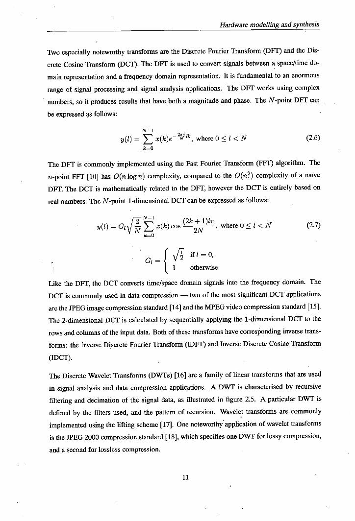
Two especially noteworthy transforms are the Discrete Fourier Transform (DFT) and the Dis-
crete Cosine Transform (DCT). The DFT is used to convert signals between a space/time do-
main representation and a frequency domain representation. It is fundamental to an enormous
range of signal processing and signal analysis applications. The DFT works using complex
numbers, so it produces results that have both a magnitude and phase. The N-point DFT can
be expressed as follows:
N-i 21 1k
Y(j) = x(k)e N , where 0 < I <N (2.6)
k=O
The DFT is commonly implemented using the Fast Fourier Transform (FIT) algorithm. The
n-point FF1' [10] has O(n log n) complexity, compared to the 0(n2 ) complexity of a naïve
DFT. The DCT is mathematically related to the DFT, however the DCT is entirely based on
real numbers. The N-point 1-dimensional DCT can be expressed as follows:
C2 N-i
where 0 < 1 < N (2.7) y(I) , x(k) (2k + l)fr
2N k=O
G1={ifl=0,
1 otherwise.
Like the DFT, the DCT converts time/space domain signals into the frequency domain. The
DCT is commonly used in data compression - two of the most significant DCT applications
are the JPEG image compression standard [14] and the MPEG video compression standard [15].
The 2-dimensional DCT is calculated by sequentially applying the 1-dimensional DCT to the
rows and columns of the input data. Both of these transforms have corresponding inverse trans-
forms: the Inverse Discrete Fourier Transform (IDFT) and Inverse Discrete Cosine Transform
(IDCT).
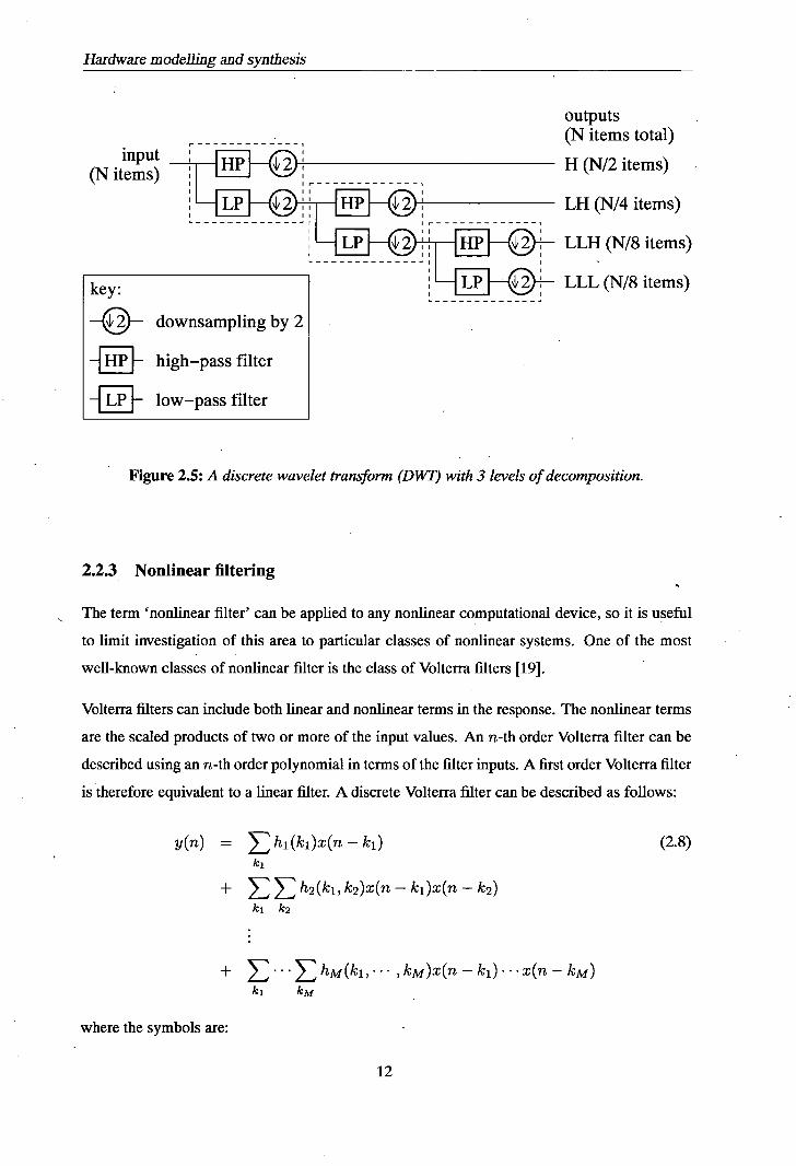
The Discrete Wavelet Transforms (DV,/Ts) [16] are a family of linear transforms that are used
in signal analysis and data compression applications. A DWT is characterised by recursive
filtering and decimation of the signal data, as illustrated in figure 2.5. A particular DWT is
defined by the filters used, and the pattern of recursion. Wavelet transforms are commonly
implemented using the lifting scheme [17]. One noteworthy application of wavelet transforms
is the JPEG 2000 compression standard [18], which specifies one DWT for lossy compression,
and a second for lossless compression.
11
Hardware modelling and synthesis
input (N items)
IL L LP 2 HP 2II
outputs (N items total)
H (N/2 items)
LH (N/4 items)
LLH (N/8 items)
LLL (N/8 items)
Figure 2.5: A discrete wavelet transform (DWT) with 3 levels of decomposition.
2.2.3 Nonlinear filtering
The term 'nonlinear filter' can be applied to any nonlinear computational device, so it is useful
to limit investigation of this area to particular classes of nonlinear systems. One of the most
well-known classes of nonlinear filter is the class of Volterra filters [19].
Volterra filters can include both linear and nonlinear terms in the response. The nonlinear terms
are the scaled products of two or more of the input values. An n-th order Volterra filter can be
described using an n-th order polynomial in terms of the filter inputs. A first order Volterra filter
is therefore equivalent to a linear filter. A discrete Volterra filter can be described as follows:
y(n) = hi(ki)x(m—ki)
(2.8) k1
+ >>h2(ki,k2)x(n—ki)x(n— k2) k1 k2
+ ,kM)x(n—kl) ... x(n—km) k1 km
where the symbols are:
12

Hardware modelling and synthesis
h(k1,... , k r,) pth-order Volterra kernel
YO output values
x(.) input yalues
The nonlinear terms in equation 2.8 exhibit symmetry, which can be used to eliminate many
of the coefficients. For example, the coefficients h2 (0, 1) and h2 (1,0) are both multiplied by
x(0)x(1), so one of these two coefficients can be eliminated. The same principle applies for
any reordering of the variables k 1 . kij.
Non-polynomial functions can often be approximated using a Taylor series, which can then be
realised as a Volterra filter. For example, a sine function can be approximated by the following
series: X3 x 5 x 7
s1n(x)x—+ j--j-+... (2.9)
which can be implemented as a Volterra filter.
23 Filter implementation
2.3.1 Hardware implementation of linear components
add input A-
°:::
- output input
carry shift
input clock—i
re—label
bit 7 bit 10 input _____
bit 0 bit 3 _______ _______output
input A
add
output
Figure 2.6: Three implementations of A + 8B. Clockwise from top left: bit-serial, 4-bit digit-serial, and bit-parallel.
Three ways of implementing the same linear function are shown in figure 2.6. A bit-parallel
implementation uses a separate wire for each data bit, while bit-serial implementations use 1-
bit components and process data items one bit at a time. Digit-serial represents a compromise
between bit-parallel and bit-serial. Digit-serial systems divide a data item into several multi-
1 13

Hardware modelling and synthesis
bit digits, and then process the digits sequentially. Bit-serial implementations are more area-
efficient, while bit-parallel designs offer higher performance.
In binary arithmetic, a left-shift of n bits is equivalent to a multiplication by 2, where n e Z.
In bit-parallel arithmetic, constant shifts can be performed at no cost, as they merely represent
a re-labelling of the bits in a value. In bit-serial arithmetic, a left-shift of one bit is equivalent
to a delay of one cycle, so one register is required for each bit of left-shift. As bit-serial shifts
are implemented using registers, they can reduce the longest-path delay. Shifts in digit-serial
designs are implemented using a combination of registers and bit re-labelling. Right-shifts are
not possible in bit-serial or digit-serial implementations.
2.3.2 Carry-save arithmetic
A carry-save adder has three inputs and two outputs. It does not propagate carries, but instead
has separate outputs for all of the sum bits and all of the carry bits. The delay through a carry-
save adder is the same as the delay through a single full adder. A carry-save adder with inputs
x, y, z, sum output s, and carry output c, can be characterised as follows:
S + • C = X + y + z
A circuit based upon carry-save adders will usually include a fast conventional adder before
each output, so that the final sum and carry values can be added together.
Figure 2.7 shows how a carry-save adder (CSA) can be used together with a ripple adder to sum
three values. A high-level diagram is shown in the left of figure 2.7, while the right-hand side
shows the same thing decomposed into half- and full-adders.
Carry-save arithmetic can be used together with shifts, provided that the sum and carry output
from each carry-save adder are scaled by the same amount prior to the final addition. Carry-save
arithmetic is therefore a useful technique for the realisation of linear circuits.
2.3.3 Multipliers and multiplication blocks
A multiplier takes two inputs and multiplies them. If one of the inputs is a constant, then a con-
stant multiplier can be used. Constant multipliers are typically more hardware efficient, where
efficiency is measured in terms of power, silicon area or latency. The design of a constant mul-
14

Hardware modelling and synthesis
Eti1Et
x[3] y[31 z[3]
x[2] y[2] z[2]
X[1]
y[ 1I Z[11
X[O]
YE0 ' Z[01
t[5]
t[4]
t[3]
t[2]
t[ 1]
t[O]
Figure 2.7: The summation of three values using carry-save arithmetic.
tiplier depends upon the constant. There are several algorithms for designing efficient constant
multipliers, starting with the value of the constant.
The simplest algorithm is the binary multiplier [20], which corresponds to the binary version
of long multiplication. A binary multiplier uses N - 1 adders, where N is the number of '1'
bits in the constant. For example, the multiplication of a value x by 7 can be broken down as
follows. Note that 1112 is the binary representation of 7.
111 2 .x=(1002 +102 +1)x1002.x+102.x+X=(X<<2)+(2<<1)+x
This multiplication can therefore be performed by adding together three different shifted ver-
sions of x.
A signed-digit binary number representation [21] is a number representation where the digits
in a number can take the values 1-1, 0, 11, rather than just {0, 1}. A signed-digit constant with
digits di has the following value:
2'd, for diE {-1,0,1}
(2.10)
iEZ
A common notation is that digits valued —1 are represented by T. For example, the value 3
15

Hardware modelling and synthesis
could be represented by 1101 = 1000 - 100 - 1. Note that this representation is redundant;
there can be multiple representations of a single value. For example, 3 can be represented by
11, loT, ill, 1101, 1111, 11111111, and infinitely many more representations. A minimum-
weight signed-digit (MSD) representation of a number is a signed-digit representation that has
the minimum number of non-zero digits. For the value 3, there are two minimum-weight rep-
resentations: 11 and 101. The Canonic Signed Digit (CSD) representation of a number is the
unique MSD representation that does not have any consecutive non-zero digits. CSD numbers
have on average one third fewer non-zero digits than binary numbers [22]. There is a computa-
tionally cheap algorithm for converting binary numbers into CSD representation [22,23].
If the constant is represented in a signed-digit form, a constant multiplier can be implemented
in a similar fashion to the binary multiplier. Negative digits result in the use of subtracters.
As an MSD number will typically have fewer non-zero digits than the corresponding binary
value, the number of additions and subtractions will often be lower in an MSD or CSD constant
multiplier.
As an example of CSD multiplication, note that the CSD representation of 7 is 1001, so the
corresponding multiplier can be derived as follows.
10012 . x = (10002 - 1)x = 10002 . x - x = (x << 3) - x
The CSD 7-times constant multiplier requires only one subtracter, in comparison with the two
adders required for the corresponding binary multiplier mentioned earlier.
There are several papers that describe the use of low-precision CSD multipliers for FIR filter
applications [24, 25]. The coefficients typically have two or three non-zero digits, and the re-
sulting coefficient quantisation has been shown to have a tolerable effect on the filter responses
in several test problems. Scaling of the coefficient set can sometimes reduce the number of
digits required [25].
CSD multiplication is not necessarily the most efficient technique. There are cases where
reusing a common sub-expression can result in a more efficient implementation. For an ex-
ample of this, see figure 2.8.
Bernstein [26] proposed a searching algorithm for constant multiplier design. Although Bern-
stein's algorithm was targeted at machine code implementation, it can also be used for elec-
16

Hardware modelling and synthesis
input "H <<:=—
__ 45 output
input u...•<< 2 4 40 <<3 I output
Figure 2.8: A suboptimal CSD multiplier: multiplication by 45.
tronic hardware design. The algorithm iteratively simplifies the constant through addition, sub-
traction, or factorisation. The choice of simplifying operation is made according to a recursively
calculated cost metric.
Dempster and Macleod devised the Minimised Adder Graph (MAG) algorithm [27-29]. This
simultaneously finds optimal constant-coefficient multipliers for many different constants, us-
ing an exhaustive search. As the number of components is increased, the computational time
required by the MAG algorithm grows at a greater than factorial rate. Dempster and Macleod
initially discovered optimal solutions for all constant multiplications with constants up to 12 bits
wide using the MAG algorithm. They later extended their results to all 19 bit constants [30]. An
exhaustive algorithm was also proposed by Li [31], however Dempster and Macleod claim that
Li's algorithm can produce sub-optimal results in some cases [32]. The explosive properties
of the search-space rule out the application of exhaustive algorithms to design multipliers for
arbitrarily large constants.
Many of the applications for constant multiplications require the same variable to be multiplied
by several constants. This introduces the possibility that intermediate values can be shared
between the multipliers, resulting in further hardware savings. The problem of designing a
multiplication block that multiplies a single variable by several constants is known as the Mul-
tiple Constant Multiplication (MCM) problem. Efficient multiplication blocks are particularly
useful for the implementation of transposed form FIR and IIR filters. For example, all of the
multiplications in the transposed form FIR shown in figure 2.2 can be combined into a single
multiplication block.
Bull and HorTocks [33] introduced four greedy search algorithms for the design of multiplica-
tion blocks, where the choice of algorithm depends upon which types of component are avail-
17

Hardware modelling and synthesis
able. The last of the four algorithms proposed by Bull and Horrocks uses adders, subtracters
and shifts, so it is the most relevant to digital circuit design. This algorithm was improved by
Dempster and Macleod [34,35].
(a) coefficient A: 1 0 1 0 0 1 1 1 = Y+100
coefficient B: 110 10 1011= y+10000 1000
where y = 10100011
(b) 001 = x+(x<.cz8)+10000
where x= 1001
Figure 2.9: Common sub-expression elimination.
Many algorithms for the design of multiplication blocks are based upon the concept of common
sub-expression elimination (CSE). A simple but inefficient implementation is found, and an
efficient implementation is then derived through the elimination of duplicated hardware. In
many cases, the coefficients for a multiplication block are represented in a binary or signed-
digit form, and common sub-expression elimination is applied in cases where similar patterns
of digits appear. This is illustrated in figure 2.9. The eliminated sub-expression can be a
bit-pattern that appears in two coefficients (figure 2.9(a)), or a repeated bit-pattern in a single
coefficient (figure 2.9(b)).
Potkonjak et al. [36] proposed the iterative matching algorithm, which is one of the most well-
known CSE-based approaches. This is a greedy algorithm which iteratively finds cases where
two signed-digit coefficients have two or more identical bits. The hardware for multiplying by
the identical bits can then be shared, as shown in figure 2.9(a). A weakness of the iterative
matching algorithm is that it does not eliminate common sub-expressions which are shifted rel-
ative to each other - for example it would not share hardware between the coefficients 11012
and 110102. The iterative matching approach led to the development of several similar algo-
rithms [37-39]. Mehendale etal. developed an algorithm which is similar to iterative matching,
but is also capable of eliminating repeated bit patterns within one coefficient [37]. The hier-
archical clustering algorithm developed by Matsuura et al. [38] can eliminate sub-expressions
between coefficients, even if they are shifted relative to each other. Pako et aL proposed a
system that can eliminate shifted multibit subexpressions across many coefficients [39]. Hart-
18

Hardware modelling and synthesis
ley's algorithm can perform common sub-expression elimination on a FIR filter implemented
using CSD coefficients [40,41]. It can eliminate sub-expressions that are relatively shifted
and delayed. Hartley's system attempts to minimise the number of registers. The NR-SCSE
system [42] is based upon Hartley's system, but also attempts to minimise logic depth. Park
and Kang [43,44] proposed a CSE-based method that makes use of the fact that there can be
multiple minimal signed-digit representations for a number. They claim this leads to increased
efficiency relative to other systems ([36,39,40]).
Dempster and Macleod's RAG-n algorithm [34] designs multiplication blocks. It builds upon
their MAG algorithm for optimal multiplier design. The RAG-n algorithm does not perform
common sub-expression elimination, and it considers a larger variety of designs when compared
with CSE-based methods. In other words, RAG-n performs a more thorough search, and the
size of the search space is correspondingly large. In many cases the RAG-n algorithm can
produce optimal results, however for some coefficient sets a fast sub-optimal search is used.
The algorithm works by generating hardware for the coefficients, one coefficient at a time. It
first generates hardware for the coefficients that are easiest to realise. When hardware for a
new coefficient is inserted into the design, the algorithm attempts to reuse as much hardware as
possible, by building upon pre-existing intermediate values.
2.3.4 Linear transforms
In [36], a variation of the iterative matching algorithm which is capable of generating hardware
for multiplication-free linear transforms was proposed. A multiplication-free linear transform is
a linear transform with coefficients limited to the values { —1, 0, 1 }. A general linear transform
can be created by using the basic iterative matching algorithm to perform the multiplications in
each column of the transformation matrix, and then summing the rows using a multiplication-
free linear transform. This is illustrated in figure 2.10.
Dempster et al. introduced an algorithm for the realisation of linear transforms [45]. It is based
upon the results of the MAG algorithm [27]. The new algorithm is compared against equivalent
hardware produced using multiple invocations of the RAG-n algorithm [34]. The results are
mixed; the new algorithm seems to be superior for smaller problems, while RAG-n is superior
if the matrix size or the precision is greater. The authors note that one option is to use the best
result from the two different algorithms.
19

Hardware modelling and synthesis
original transform
90 117 '90 49
~ Y1
\
Y2 ( 90 49 —90 —117
~yj 90 —49 —90 117 1 3 (90)x1
y \ 90 —117 90 —49 / \x4 /
$ 1 (49 )# (90)x1 (90)x3
117
(90)x3 49
(117 ) x2 ( 4 )x4 I 49\ I\ 117)
X4
multiplication block for each column
multiplication—free transform / 90X,
(
/y1 101110 /49x2 (y2 1 1 0 —1 0 -11 117x2
1 —1 0-1 0 1 90x3 \y4 / \ 1 0 —1 1 —1 0 1 \ 49;
117;
Figure 2.10: Designing linear transform hardware using the iterative matching algorithm.
In [46], Chatterjee et al. proposed several common subexpression elimination methods for
matrix multiplications, together with a greedy algorithm that iteratively applies these optimisa-
tions.
Transform-specific optimisations are often devised for important transforms. The higher-level
optimisation methods attempt to minimise the number of multiplications. The most famous
example of this is the use of the Fast Fourier Transform (FF1) algorithm [10] for the discrete
Fourier transform (DFT). Chen et aL [47] proposed a technique for efficiently calculating the
DCT. This method can be used to calculate the 8-point 1-dimensional DCT using 16 multiplies
and 26 additions/subtractions. Loeffler et al. devised an algorithm which can perform an 8-
point DCT using 11 multiplications and 29 additions [48]. Arai et al. [49] proposed a method
which is more efficient if scaling of the DCT outputs does not matter. The algorithm uses
5 multiplications and 27 additions for the 8-point DCT. There are also several multiplierless
approximations to the DCT, based upon the lifting scheme [50-53]. The complexity of fixed-
point approximations to the DCT varies depending on the accuracy, so direct comparisons
between these methods are not always possible.
20
Hardware modelling and synthesis
The inverse DCT can be realised using the transposition [11] of any DCT implementation. It
was found that the complexity of a particular DCT implementation and its transpose are always
identical, as the number of branches in the transform's flowgraph is always equal to the number
of additions [14]. Therefore, every efficient DCT algorithm can be converted to an efficient
IDCT algorithm.
2.3.5 Existing linear filter design systems
While section 2.3.3 described several different algorithms for the design of efficient multiplica-
tion blocks, there are also tools that use those algorithms during the creation of complete filter
designs. FIRGEN [54] is an FIR filter design system that converts a filter specification into a
chip layout. FIRGEN generates CSD multiplication blocks. Wacey and Bull implemented the
POFGEN filter design system [55], which is based around the algorithms introduced in [33].
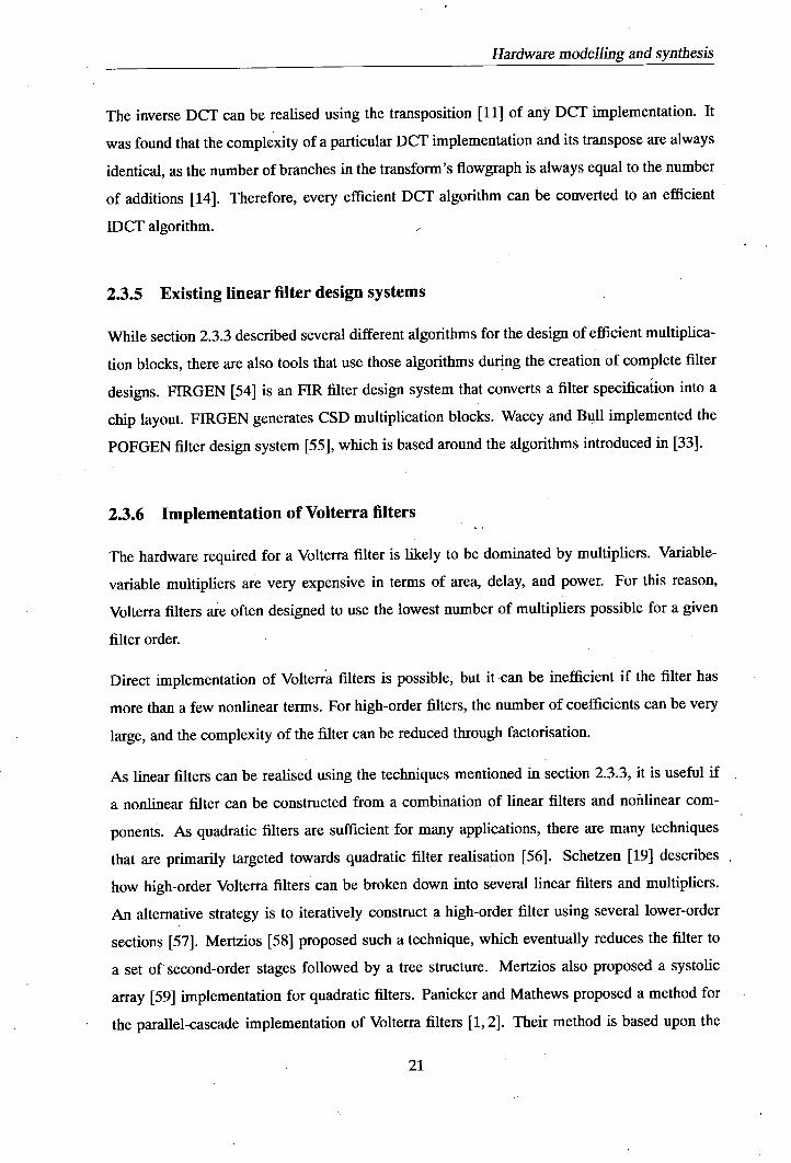
2.3.6 Implementation of Volterra filters
The hardware required for a Volterra filter is likely to be dominated by multipliers. Variable-
variable multipliers are very expensive in terms of area, delay, and power. For this reason,
Volterra filters are often designed to use the lowest number of multipliers possible for a given
filter order.
Direct implementation of Volterra filters is possible, but it can be inefficient if the filter has
more than a few nonlinear terms. For high-order filters, the number of coefficients can be very
large, and the complexity of the filter can be reduced through factorisation.
As linear filters can be realised using the techniques mentioned in section 2.3.3, it is useful if
a nonlinear filter can be constructed from a combination of linear filters and nonlinear com-
ponents. As quadratic filters are sufficient for many applications, there are many techniques
that are primarily targeted towards quadratic filter realisation [56]. Schetzen [19] describes
how high-order Volterra filters can be broken down into several linear filters and multipliers.
An alternative strategy is to iteratively construct a high-order filter using several lower-order
sections [57]. Mertzios [58] proposed such a technique, which eventually reduces the filter to
a set of second-order stages followed by a tree structure. Mertzios also proposed a systolic
array [59] implementation for quadratic filters. Panicker and Mathews proposed a method for
the parallel-cascade implementation of Volterra filters [1, 2]. Their method is based upon the
21

Hardware modelling and
r.J
x(n)
y(n)
Figure 2.11: The decomposition of a Volterra filter proposed by Panicker and Mathews[1, 4.
recursive decomposition of a pth order filter into multiple filters of order 1 and order p - 1. This
is shown in figure 2.11. Panicker and Mathews also investigate the inaccuracies introduced in
truncated representations of these filters.
The frequency domain analysis of nonlinear filters is a well established field [19]. Techniques
which are based upon a frequency domain representations of the filter [60, 61] can also be. used
for filter implementation. The Fast Fourier Transform (FFT) and inverse Fast Fourier Transform
can then be used to move between the time/space domain and the frequency domain. The com-
bined operation is sometimes more efficient than a direct implementation. This methodology
can also be used with transforms other than the Fourier transform [60].
2.4 Hardware properties and modelling
This section investigates the ways in which the hardware described in section 2.3 can be mod-
elled. Modelling is of interest because it is essential for evlutionary circuit design. Therefore,
this section focusses on modelling the circuit properties that can usefully serve as objectives
during evolutionary circuit design.
22

Hardware modelling and synthesis
2.4.1 Pre-placement modelling
The properties of a digital hardware design are heavily influenced by the particular placement
and routing that is applied. This is particularly relevant to clock speed, power consumption, and
circuit area. The properties of a design can be accurately modelled after placement and routing,
however placement and routing are complex, computationally expensive tasks. It is common for
placement and routing problems to be NP-complete [62,63]. Even non-optimal placement and
routing systems necessarily work with a very detailed low-level design representation, leading
to high computational costs. It is therefore often desirable to able to estimate the properties of
a design prior to placement and routing. This is possible through the use of statistical models.
2.4.2 Wire-load modelling
(a) V o—LIIIiJ---i VOUT IN
T T T
R
(b) VINo I VOUT
C
Figure 2.12: Two wire load models.
A wire on a chip can be characterised as a distributed resistance connected to the substrate by
a distributed capacitance [64]. Figure 2.12 illustrates two models of this. The transmission
line model shown in figure 2.12(a) is an accurate representation of the properties of the wire,
however a simplified model such as figure 2.12(b) can be sufficiently accurate for most prac-
tical power or delay simulation. The loads in a CMOS device are transistor gates, which are
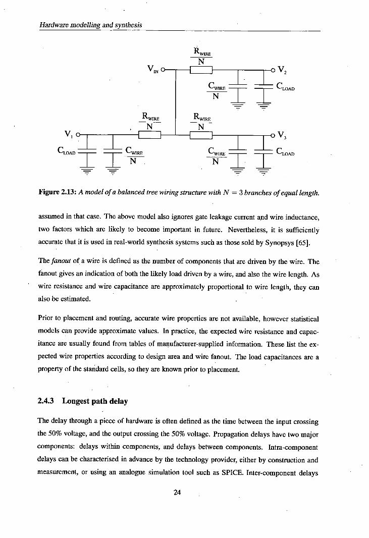
largely capacitive. Assuming that the wire is a balanced tree, with branches of equal length, the
combined model in figure 2.13 can be used [65].
The above model makes several simplifying assumptions. In particular, the shape of the wire
and the distribution of the loads are not known prior to placement and routing, so they must be
23
Hardware modelling and synthesis
IN
V1
V2
CLOAD
V3
CLOAD - WIRE
IN •W1RE
NI
Figure 2.13: A model of a balanced tree wiring structure with N = 3 branches of equal length.
assumed in that case. The above model also ignores gate leakage current and wire inductance,
two factors which are likely to become important in future. Nevertheless, it is sufficiently
accurate that it is used in real-world synthesis systems such as those sold by Synopsys [65].
The fanout of a wire is defined as the number of components that are driven by the wire. The
fanout gives an indication of both the likely load driven by a wire, and also the wire length. As
wire resistance and wire capacitance are approximately proportional to wire length, they can
also be estimated. -
Prior to placement and routing, accurate wire properties are not available, however statistical
models can provide approximate values. In practice, the expected wire resistance and capac-
itance are usually found from tables of manufacturer-supplied information. These list the ex-
pected wire properties according to design area and wire fanout. The load capacitances are a
property of the standard cells, so they are known prior to placement.
2.4.3 Longest path delay
The delay through a piece of hardware is often defined as the time between the input crossing
the 50% voltage, and the output crossing the 50% voltage. Propagation delays have two major
components: delays within components, and delays between components. Intra-component
delays can be characterised in advance by the technology provider, either by construction and
measurement, or using an analogue simulation tool such as SPICE. Inter-component delays
24

Hardware modelling and synthesis
depend upon the properties of the driver, interconnect, and load.
input RA RB © R output
VIN VOUT
T C, 1C2 1C3
R
RB © C3
inp:tRA
R C2 I RE
D
C4
_
RF
I _ - Có ::
Figure 2.14: Elmore delay models for (a) a chain of RC delays and (b) a tree of RC delays with
a single driver.
RC delays are commonly used in delay modelling. They let the delay model take account of
the electronic properties of the circuit, without introducing excessive computational complexity.
Elmore delays [66] are a useful technique for estimating the overall delay produced by a net-
work of resistances and capacitances. The Elmore delay for the network shown in figure 2.14(a)
is given by:
TD= RC, (2.11)
where R is the sum of the resistances between the input and node i. For tree-structured net-
works, such as the network in figure 2.14(b), the Elmore delay for node i can be calculated as
follows [67]:
Tj=>RjjCj (2.12)
25
y[2]
All (c)
Y101
y[3:2]
Y[1:0]
x[3:2]
X[1:0]
x[2]
(b)
X[1]
x[0]
Hardware modelling and synthesis
where R 3 is the sum of the resistances in the part of the tree driving both nodes i and j [68-70].
For example in figure 2.14(a), the delay between the input and the output is estimated as:
TD = RAC1 + (RA + RB)C2 + (RA + RB + R)C3 (2.13)
The delay between the input and node 4 in figure 2.14(b) can be modelled as:
T4=RA(Cl+C2+C3)+ (RA +RD)(C4+C5+C6) (2.14)
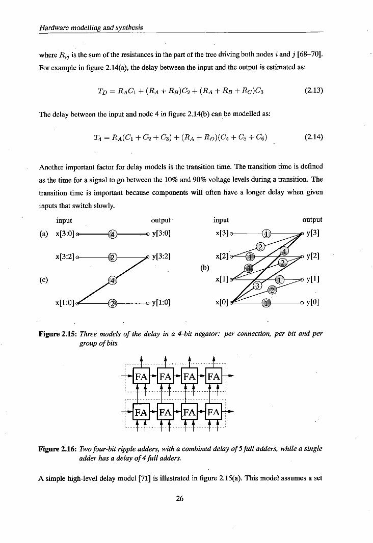
Another important factor for delay models is the transition time. The transition time is defined
as the time for a signal to go between the 10% and 90% voltage levels during a transition. The
transition time is important because components will often have a longer delay when given
inputs that switch slowly.
input output input output
(a) x[3:0]0 oy[3:0] x[3]o ED y[3]
Figure 2.15: Three models of the delay in a 4-bit negator: per connection, per bit and per group of bits.
Figure 2.16: Two four-bit ripple adders, with a combined delay of full adders, while a single adder has a delay of full adders.
A simple high-level delay model [71] is illustrated in figure 2.15(a). This model assumes a set
Wei

Hardware modelling and synthesis
of constant delays between the inputs and outputs of the high-level components. This model
is often inaccurate due to skewing of the arrival times for individual bits. An example of this
problem is shown in figure 2.16. The problem can be avoided if the model instead considers
delays between individual bits [71,72], as shown in figure 2.15(b). Computing delays for
individual bits is a computationally intensive task, so one possibility is that delays can instead
be computed for groups of bits [721, as shown in figure 2.15(c). Wire-load modelling can also
be important for high-level delay modelling.
2.4.4 Power
Power consumption can be split into static and dynamic power consumption. In current CMOS
technologies, the power consumption is dominated by dynamic power consumption. Static
power consumption is likely to become more significant in future technologies [73]. Dynamic
power consumption is caused by signal transitions, so it is data-dependent.
Transitions are often a result of glitching. During one cycle of a computation a signal can
change state several times before assuming a correct value. This happens because of unequal
signal propagation delays. Glitching can be a notable cause of power dissipation.
As power consumption is strongly related to the number of signal transitions, the most accurate
power models are based upon circuit simulation, and use a representative sample of the circuit
inputs. These models are typically accurate but computationally expensive. Alternatively, a
power model can be based upon a statistical model of the input data. These models are typically
computationally cheaper than a full simulation, but give less accurate results. The simplest
power models ignore the effects of the input data on power consumption.
VDD
ILOAD
rT - --------- II
JSHORT R
_L Figure 2.17: Dynamic power consumption in a CMOS inverter.
The dynamic power consumption of a CMOS circuit can be estimated using the model shown
27

Hardware modelling and synthesis
in figure 2.17. The power consumption is a combination of the power used to drive the load,
and the short circuit power consumption that occurs when the pull-up and pull-down transistors
simultaneously conduct during switching. CMOS transistors are usually designed so that short-
circuit power consumption is largely avoided, and it is often ignored in power simulations. The
power dissipation due to the charging and discharging of the load capacitance can be expressed
as follows:
P = CV Df (2.15)
where C is the load capacitance, lID is the supply voltage, and f is the transition frequency.
Therefore, the power dissipation can be approximated if the capacitance and transition fre-
quency is found for each wire in the design.
Power dissipation can be estimated by simulating the design, and counting the transitions on
each wire. The transition counts and estimated capacitances can then be used in equation 2.15,
giving the overall power estimate [74]. This method is accurate, but also computationally
expensive. Other computationally cheaper approaches attempt to estimate the power dissipation
according to the high-level properties of the design.
Power dissipation is related to design area. The chip estimation system (CES) model [75]
calculates power as follows:
P GE(E + VDDCL)fAiTht (2.16)
where GE. is the area in gate equivalents, Etyp is the energy consumed by a typical gate, CL
is the average load, f is the frequency of operation, and Ai,, t is the activity. Aint represents
the proportion of gates that transition in an average clock cycle. Liu and Svensson described
a similar system, which divides components into several classes, where each class has distinct
properties [76]. The Power Factor Approximation (PFA) technique [77] estimates the power
used by hardware components relative to other similar components. It can be stated as follows:
P = kGf (2.17)
where k is a constant, f is the frequency of operation. C is measure of complexity specific to
the class of components. For example, for n-bit multipliers C = n2 . This style of analysis
was later investigated in greater depth by the same authors [78]. A major weakness of these
high-level techniques is that they ignore the fact that power dissipation is very data dependent.
003
- Hardware modelling and synthesis
The dual bit type (DBT) model of power consumption [79] divides data items into upper and
lower bits. The former represent sign bits which transition whenever the sign of a value is
changed, while the latter are data bits that can be modelled using uniform white noise. This
division allows different switched capacitance activity models to be used for each class of bits.
The DBT model can be used together with high-level components that have a known power
consumption for each type of bit.
Other power estimation techniques include those that treat switching activity as a form of en-
tropy [80,81], table based methods [82-84], and methods based on statistical regression in
terms of the input variables [85]. Many other power estimation systems are described in a
number of review papers [86-88].
2.4.5 Silicon area
The silicon area required for a circuit is a function of two different areas - the area used by
components (cell area) and the area used by interconnects (net area). The cell area can be found
from the type and number of cells in a design. The net area depends upon how the interconnects
are routed. The net area can be approximated prior to routing according to a statistical model
of the likely area taken by each wire. The expected area for a wire can be deduced according
to the fanout of the wire and the area of the design. This method of area estimation is sup-
ported by real synthesis systems [65]. Unfortunately, the necessary data is not always present
in technology libraries. Alternative ways of estimating the net area include constructive meth-
ods [89] or analytic methods [90,91]. These techniques offer increased accuracy, but also have
more parameters. Constructive methods in particular can produce very accurate results, but are
computationally expensive and require extensive knowledge of a technology.
2.4.6 Other metrics
Finite precision arithmetic can introduce round-off noise into the response of a digital system.
Round-off noise is-nonlinear and data-dependent. It is commonly expressed as a signal to
noise ratio (SNR). While the SNR can be calculated through simulation, the use of statistical
models [92] is more practical. This thesis does not investigate the problems caused by finite
arithmetic precision.
A testability metric measures how well a particular design can be used together with the built-
29

Hardware modelling and synthesis
in self-test (BIST) techniques, required in modern chips. Testability is often measured at a
low-level [93]. These low-level metrics are based around the evaluation of the observability
and controllability of each node in a design. There are also some useful high-level testability
measures, which are based on similar principles [94, 95].
Routability metrics assess how amenable to placement and routing a particular design is. Rout-
able designs are likely to have shorter interconnects. A routability metric will therefore indicate
how optimistic or pessimistic preplacement area, delay and power estimates are likely to be.
Routability can be assessed prior to routing [96, 97], or else during hierarchical routing [98].
2.5 Summary
This chapter has described various techniques for the design, implementation and modelling
of digital filters. It has documented various ways in which hardware efficient filters can be
designed. This information will be used in later chapters.
It was noted that filter designs can be made more efficient through the use of primitive opera-
tors such as adders and shifters, and by reusing intermediate results. Optimal filter realisation
is'often an intractable problem. In several cases, this has led to the development of greedy
algorithms and partial searches for near-optimal filter design.
Interconnect modelling was shown to be a major source of inaccuracy when modelling ASIC
hardware. Area, delay, and power models all depend upon the properties of the interconnects,
which cannot be reliably estimated prior to placement and routing. Statistical models enable
rapid wire modelling, however they have a limited accuracy.
Accurate hardware models are often computationally intensive. A practical approach to mod-
elling should trade between accuracy and computational complexity as required.
WE

Chapter 3 Evolutionary algorithms and stochastic search techniques
3.1 Introduction
Many important CAD problems have large multiinodal search spaces, so robust search tech-
niques are essential. Evolutionary algorithms are an appropriate search technique for applica-
tion to some of the hardest digital hardware synthesis problems.
This chapter describes evolutionary algorithms and other stochastic search techniques, and in-
vestigates how they relate to electronics. Section 3.2 gives a brief overview of some of these
search techniques. Section 3.3 demonstrates how these techniques can be applied to multiob-
jective searches with conflicting objectives. Section 3.4 describes how evolutionary methods
can be used to design electronic circuits, and digital filters in particular.
3.2 Evolutionary algorithms
The term 'evolutionary algorithm' can be used to describe algorithms from a large set of biolog-
ically inspired stochastic search techniques. The major features of EAs are mutation, hybridis-
ation, and selection, iteratively performed on a population of solutions. Although evolutionary
algorithms are frequently compared with natural evolution, a more accurate analogy would be
the selective breeding of plants or animals. Both evolutionary algorithms and selective breeding
work upon a population, and attempt to achieve improvements in the population by repeatedly
favouring the reproduction of population members that have desired characteristics.
Evolutionary algorithms can be classified into several groups, which often overlap. The most
significant groupings are: genetic algorithms, evolutionary programming, evolution strategies,
and genetic programming. Evolution strategies are for continuously valued problems, so will
not be discussed in this thesis. Many EAs have features associated with two or more of the
above categories.
31
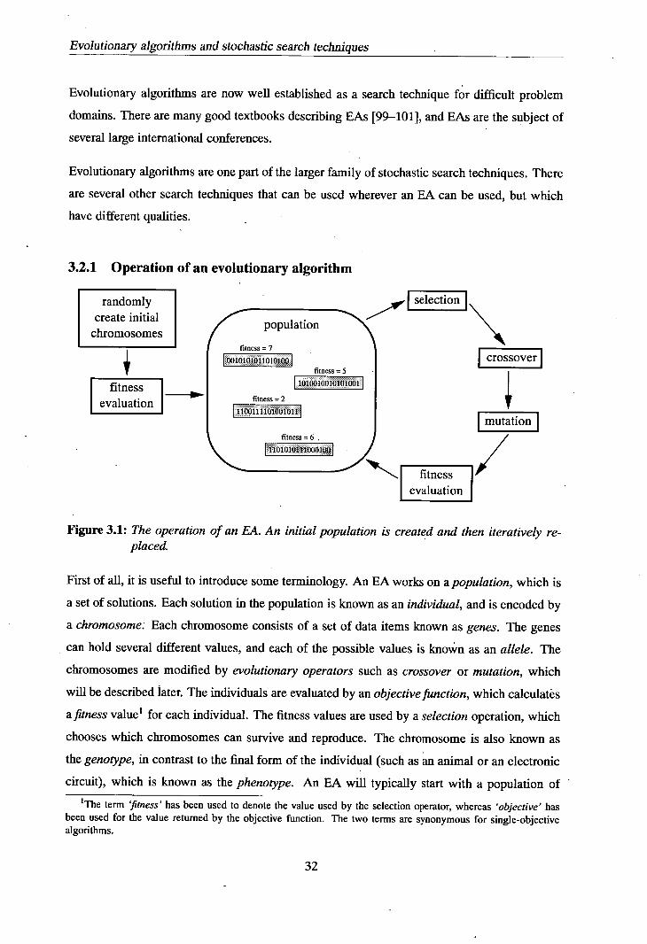
Evolutionary algorithms and stochastic search techniques
Evolutionary algorithms are now well established as a search technique for difficult problem
domains. There are many good textbooks describing EAs [99-101], and EAs are the subject of
several large international conferences.
Evolutionary algorithms are one part of the larger family of stochastic search techniques. There
are several other search techniques that can be used wherever an EA can be used, but which
have different qualities.
3.2.1 Operation of an evolutionary algorithm
randomly create initial
chromosomes
fitness evaluation
-
population F = 7
101i)1( fltness=5
101 [1011)010101001
fitness = 2
iiiüöiooioti
fitness = 6
I: fl 110 1110 011)1)
selection I
crossover
Fulation
fitness / evaluation
Figure 3.1: The operation of an EA. An initial population is created and then iteratively re-placed.
First of all, it is useful to introduce some terminology. An EA works on a population, which is
a set of solutions. Each solution in the population is known as an individual, and is encoded by
a chromosome; Each chromosome consists of a set of data items known as genes. The genes
can hold several different values, and each of the possible values is known as an allele. The
chromosomes are modified by evolutionary operators such as crossover or mutation, which
will be described later. The individuals are evaluated by an objective function, which calculates
a fitness value' for each individual. The fitness values are used by a selection operation, which
chooses which chromosomes can survive and reproduce. The chromosome is also known as
the genotype, in contrast to the final form of the individual (such as an animal or an electronic
circuit), which is known as the phenotype. An EA will typically start with a population of
'The term 'fitness' has been used to denote the value used by the selection operator, whereas 'objective' has been used for the value returned by the objective function. The two terms are synonymous for single-objective algorithms.
32

Evolutionary algorithms and stochastic search techniques
randomly generated chromosomes. It then iteratively improves the population. Each iteration
is known as a generation. The cycle at the right of figure 3.1 shows the operations that a
simple EA uses to progress one generation. The algorithm stops either after a set number of
generations, or else when the population is judged to be of satisfactory quality.
Selection is the process of choosing chromosomes, either for reproduction or for survival. EM
typically use a stochastic selection operator, where the fittest individuals have the highest prob-
ability of selection. The three most common selection operators are: rank proportionate, fit-
ness proportionate, and tournament selection. Fitness proportionate selection is also known
as roulette wheel selection. In size-n tournament selection, n individuals are picked from the
population at random, and entered into a tournament. The winner of the tournament is the in-
dividual with the highest fitness, and the winner is selected. The fittest individual will win any
tournament it is selected for, while the worst individual can only win if it is selected n times
for the same tournament. The probability of selection in a tournament is therefore dependent
on rank within the population.
The choice of selection scheme can have a major effect on the, performance of an EA. If the se-
lection scheme only weakly favours the best solutions, the EA can run slowly or fail to produce
a solution. If selection strongly favours the best solutions, the search becomes more greedy, and
faster, but is more likely to get stuck in a local optimum. This conflict is known as the problem
of exploration versus exploitation.
Crossover enables the creation of hybrid chromosomes, as shown in figure 3.2. Crossover takes
two (or more) parent chromosomes, and produces a child chromosome that contains some genes
from each of the parent chromosomes. Crossover therefore serves a similar purpose to sexual
reproduction in nature. In the best case, it can combine good genes from both parents resulting
in a child chromosome with a greater fitness than either parent.
Crossover
1öIiIoIoIoIiIiIiI oIiIoIojoIoTj.':j _
FiIooliiliIiIiI
Mutation,
lojilolololililil -.,. roTiioriioIiIiIiI
Figure 3.2: Crossover and mutation as applied to a binary chromosome.
Mutation is the modification of some of the genes in a chromosome, as shown in figure 3.2.
OJ

Evolutionary algorithms and stochastic search techniques
The parallel in nature is the modification of DNA by radiation, chemical processes, or incorrect
replication. Mutation is useful as a search technique as it enables the creation of new genetic
material in a population.
An idea which is central to the development of EAs is the building block hypothesis. Useful
genes can arise in different individuals within a population, which can later be combined into
a single chromosome by the crossover operator. In this way, high-fitness chromosomes can be
rapidly assembled from small genetic 'building blocks'. This principle is encoded by schema
theory [99], which mathematically describes the investigation and reproduction of such building
blocks in an evolutionary search.
An elitist BA is one that explicitly preserves the best chromosomes. The set of preserved
chromosomes is known as the elite. Elitism is intended to prevent the wasteful elimination of
good genes. Elitism can aid the rapid discovery of high-quality chromosomes, however it can
also be detrimental in some cases. Elitism is effectively an extra form of selection that rewards'
the best individuals in the population. Alternatively, elitism can be considered to be a form of
evolutionary punishment for non-elite individuals; non-elite individuals are more likely to be
displaced by the elite and their relatives. Elitism theref6re trades the preservation of good genes
in the elite, against the loss of good genes from the non-elite.
3.2.2 Fitness landscapes
If a chromosome has n genes, then the fitness could theoretically be found for every combina-
tion of alleles, resulting in a fitness 'landscape' in ii + 1 dimensional space. The shape of this
landscape indicates how hard the problem is; if the landscape is smooth, the problem is likely
to be simple. If the fitness landscape is rough and has a large number of peaks and valleys, the
problem is likely to be harder to solve. If the fitness landscape is rough, an explorative search
algorithm is necessary, otherwise the search is likely to become stuck at a local optimum. In
contrast, greedier searches perform better if the landscape is relatively smooth and there is little
benefit in exploring.
The interaction of different genes in a chromosome is known as epistasis. The degree of epis-
tasis can be used to measure the roughness of the fitness landscape, and hence the complexity
of the problem. Kauffman proposed the NK model of fitness landscapes [102]. The NK
model describes an entity with N components (genes), where the fitness contribution from
34

Evolutionary algorithms and stochastic search techniques
each component depends upon K other components. Rugged fitness landscapes can therefore
be modelled using an NK model where K is large.
3.23 A taxonomy of evolutionary algorithms
3.2.3.1 Genetic algorithms
Genetic algorithms were originally devised by Holland [103]. The features that typify a genetic
algorithm are the use of crossover as the major evolutionary operator, and the use of a linear
binary encoding for the chromosome. Genetic algorithms use mutation as a minor operator,
which is intended to aid the application of crossover.
3.2.3.2 Evolutionary programming
Evolutionary programming (EP) was invented by Lawrence Fogel in the 1960's. It was origi-
nally applied to the design of Finite State Machines (FSM5) [104]. EP does not use crossover,
and uses mutation as the sole evolutionary operator.
In contrast to GAs, EP is more robust where there is a high level of epistasis. Crossover tends
to be destructive when applied to epistatic chromosomes, as it interferes with a large number
of relationships between genes. Mutation causes only local changes, so it is less likely to be
damaging.
3.2.3.3 Genetic programming
Genetic programming (GP) was originally described by Koza [105]. It uses a chromosome
encoding that is based upon trees of expressions. GP was originally used for the creation of
computer programs, interpreting the chromosomes as S-expressions 2 in the LISP programming
language. The major operator used by GP is crossover, which is performed by cloning the
parents, randomly selecting a subtree in each clone, and swapping the subtrees. The chro-
mosome encoding used by GP is relatively expressive, and has been applied to a variety of
problems [105].
Koza developed an extension to genetic programming known as automatically defined functions
2 An S-expression is a representation for a tree of LISP operators and operands. Every program or expression in LISP is represented as an S-expression.
35

Evolutionary algorithms and stochastic search techniques
(ADFs) [106]. An ADF is a sub-expression which can be repeatedly referenced elsewhere in
the chromosome. This is similar to the use of function calls in programming languages. ADFs
are useful because they enable the rapid evolution of repeating features in the phenotype.
3.2.4 Other stochastic search techniques
Hill-climbing is a greedy search technique. It works on a single solution. At each step in the
algorithm, .the fitness values of all of the neighbours to the current solution are found. The
hill-climbing algorithm selects the neighbour solution with the highest fitness. If all of the'
neighbour solutions have lower fitness than the current solution, the algorithm stops. A hill-
climbing algorithm travels 'uphill' in the fitness landscape until it reaches an optimum in the
fitness landscape. There is no way of knowing whether it is a local or global optimum. Hill-
climbing is efficient, but not robust.
A random walk is a simple greedy search technique. It iteratively compares a current solution
with a modified version of the same current solution, and makes the better of the two into the
new current solution. Like hill-climbing, a random walk cannot distinguish between 'local and
global optima.
Simulated Annealing [1071 is a search technique that is inspired by the behaviour of atoms in
a hot metal which is being cooled. Simulated Annealing uses a parameter T, which represents
the temperature of the search. T is used in defining the probability that the current solution is
replaced with a worse solution. If T is high, the search is explorative, whereas low values of T
result in a greedy search. T is reduced over time. Simulated Annealing iteratively compares a
single current solution with modified versions of the same current solution.
Tabu search [108, 109] was invented by Glover in 1977. It is similar to a random walk, but
maintains a list of recently visited solutions known as the tabu list. A tabu search will not
revisit solutions which are on the tabu list. The use of a tabu list encourages exploration of the
search space, and avoids repeated evaluations of the same solutions.
The above searches do not make any assumptions about the properties of the solutions or the
form of the search space. It is very common to include domain-specific heuristics in a search
algorithm, resulting in a faster or more efficient search.
36

Evolutionary algorithms and stochastic search techniques
3.2.5 Hybrid search techniques
The search techniques in section 3.2.4 are generally fast but not robust. This contrasts with
EAs, which tend to be slower and more robust. It is therefore natural to want to combine these
techniques, to produce a search that is faster than an EA and which is still reasonably robust.
One simple approach is to apply a local search to the results of an EA, so that the overall solution
is definitely a local optimum. An alternative approach is to incorporate a local search into an
EA, either as an extra operation which is applied to some individuals, or else incorporated into
the evolutionary operators. In any of these hybrid schemes, the local search can potentially
incorporate application domain specific heuristics.
3.3 Multiobjective evolutionary algorithms
Multiobjective evolutionary algorithms (MOEAs) have been thoroughly researched in recent
years [110-112]. MOEAs are important because real problems often have multiple conflicting
objectives. The fact that MOEAs work with a population of solutions lets a single MOEA run
investigate the entire trade-off surface for a problem.
3.3.1 Multiobjective problem solving
A major distinction between multiobjective optimisation and single-objective optimisation is
the possibility that there might be more than one optimal solution. The set of optimal solutions
to a multiobjective problem is known as the Pareto-optimal set.
A point a in an objective space is said to dominate another point b if the following applies:
a is at least as good as b with respect to all objectives,
a is better than b with respect to at least one objective.
If a dominates b it implies that a is always better than b, regardless of which objectives are
considered most important. This is illustrated in figure 3.3. All of the problems mentioned
in this thesis are minimisation problems, so 'better' solutions have smaller objective values.
The Pareto set (Pareto surface) contains the solutions that can not be dominated by any other
solutions. Every non-Pareto solution is dominated by at least one solution in the Pareto set.
37

Evolutionary algorithms and stochastic search techniques
objective 1
b •
a •
I--- ' I----.
objective 2 key: U Solution
--- Pareto surface
Figure 33: Point a dominates point b, while both a and bare dominated by some of the points on the Pareto surface.
When dealing with a subset of the possible solutions, such as the results of a multiobjective
EA, the set of best quality solutions is known as the non-dominated set.
The non-dominated solution set produced by a multiobjective search algorithm should have
two important properties. Firstly, the non-dominated set should be as close as possible to the
Pareto set; in other words, the results should be near-optimal. Secondly, the solution set should
be as diverse as possible. Diversity can be divided into two key qualities: the non-dominated
surface should-be as broad as possible, and the solutions should be evenly distributed across the
non-dominated surface. This is shown in figure 3.4.
objective
/
objective 2
Figure 3.4: Selection pressure towards optimal solutions (solid arrows) and a diverse solution set (dashed arrows).
Many modem multiobjective ranking schemes are based upon the concept of Pareto domina-
tion. These schemes are useful because they enable the discovery of the widest variety of
solutions. Nevertheless, non-Pareto methods are useful in situations where exploration should
02

-- Evolutionary algorithms and stochastic search techniques
be limited to part of the objective space.
3.3.2 Non-Pareto ranking methods
objective 1
objective 2
Figure 3.5: A concave Pareto surface with Pareto points A, B, and C, where point B is in a
concavity.
Some MOEAs rank individuals using a weighted sum of the objectives. This is simple to
implement, but it has several disadvantages. The most significant disadvantage of this method
is that it tends to encourage the whole population to move towards one point on the Pareto
surface. A further disadvantage is an inability to adequately reward solutions on a concave
section of the non-dominated surface. For example, in figure 3.5, either point A or point C will
always be ranked higher than point B, for any choice of weights. It is possible to partially avoid
this problem by nonlinear transformation of the objective values [111].
The Vector Evaluated GA (VEGA) proposed by Schaffer [113] divides the population into
different sub-populations each generation, and performs selection in each sub-population us-
ing a different objective. Richardson et al. later found this to be equivalent to an aggregate
method [1121.
Some methods rely on a way of explicitly defining intermediate goals for evolution. Such a
system will not cover an entire trade-off surface, but will let evolution concentrate on the part
of the surface that is of most interest to the user. Fonseca and Fleming described the use of a
decision maker - an entity that sets intermediate goals during evolution [114, 115].
A lexicographic ranking [116] defines an order of precedence for the objectives. Individuals
are initially ranked according to the highest precedence objective, and, individuals that are equal
with respect to higher precedence objectives are sorted by successively lower precedence ob-
39

Evolutionary algorithms and stochastic search techniques
jectives. Lexicographic ranking does not encourage the exploration of compromises between
different objectives, but it is useful when some objectives are clearly more important than oth-
ers.
3.3.3 Pareto ranking methods
Pareto-based ranking methods are not heavily biased towards one part of the Pareto surface.
They should be used together with a method of rewarding diversity, so that the population does
not converge on one part of the trade-off surface due to factors such as genetic drift.
Fonseca and Fleming proposed a ranking scheme where the rank of each chromosome is one
more than the number of chromosomes that dominate it [114, 115]. This scheme was used in
MOGA, their multiobjective EA.
objective A
0 : U ......3 •- : : U..
21 ............ u.....
1............ 0I ---- i
0l---i
objective B key: • Individual
--- Non—dominated individuals Dominated ranks
Figure 3.6: The ranks assigned to a population by the non-dominated sorting algorithm.
Goldberg proposed the non-dominated sorting algorithm [99], which is a ranking scheme based
on domination:
let r = 0; initialise set P containing the whole population; while (P is not empty) do {
find the non-dominated set, N, for set P; assign rank r to all members of N; remove all members of N from P; let r = r + 1
}
9]

Evolutionary algorithms and stochastic search techniques
An example of the results of using this algorithm is shown in figure 3.6. Note that the non-
dominated solutions are assigned a rank of zero.
Horn et aL proposed the Niched Pareto GA (NPGA) [117]. This uses a type of tournament
selection which is based on domination. In each tournament, two candidates are chosen from
the population at random. A comparison set of individuals is also randomly picked from the
population. If one of the candidates is dominated by the comparison set, but the other is not, the
latter wins the tournament. In other cases the winner is chosen according to a diversity metric.
3.3.4 Population diversity
There are two types of diversity: variable-space (genotypic) diversity and objective-space di-
versity. MOEAs normally require results that are spread across a trade-off surface, so objective-
space diversity is essential. Genotypic diversity indicates an explorative search. There is often
correlation between these two types of diversity - in particular, genotypic diversity can lead
to diversity in the objective space.
Most MOEAs employ some kind of mechanism that explicitly encourages diversity. This coun-
teracts the tendency for the population to converge on a small area of the objective space, due
to genetic drift and variations in the fitness landscape. Two of the most common methods of
rewarding diversity are crowding and fitness sharing [99, 110]. Crowding encourages diversity
by ensuring that each new child individual replaces the most similar individual from a randomly
chosen set of pre-existing individuals. Sharing introduces a penalty for individuals that are sim-
ilar - it is designed so that n identical individuals will be given a 1/n share of the original
fitness value. Fitness sharing only occurs when individuals are less than a set distance apart,
typically defined by the parameter share• Goldberg and Richardson define a sharing function,
s(d), which is defined in terms of the distance d between two solutions [110]:
(3.1) = share s(d) { 1 - if d
0, otherwise.
The sharing function has value 1 at distance 0, and value 0 at distance Usha,. If the parameter
c is set to 1, then s(d) declines linearly with distance. s(d) Is used when calculating a niche
count ni for solution i:
n=s(dj). (3.2)
41

Evolutionary algorithms and stochastic search techniques
This is an estimate of the number of other solutions in the same evolutionary niche as solution
i. A scaled fitness value can then be calculated as follows:
fi ni (3.3)
Both of the above techniques can measure the distance between solutions in either the objective
space or the variable space.
3.3.5 Multiobjective elitism
The best individuals in an MOEA population are the non-dominated set. As the number of
objectives is increased, it becomes increasingly likely that a particular individual will be in the
non-dominated set. Many MOEAs have a limited elite size, and choose a diverse selection
of non-dominated individuals if the non-dominated set is larger than the elite size. There are
several methods for choosing a diverse elite - see [110] for examples.
3.4 Evolutionary algorithms and electronics
Digital circuit synthesis involves many complex tasks. Many of these tasks are optimisation
problems with large, multi-modal objective landscapes. Many of the optimisation problems
are computationally intractable, in which case a globally optimal solution can be unobtainable.
In addition, there are often multiple, possibly conflicting objectives. The complexity of these
problems encourages the use of powerful heuristic search algorithms, of which EAs are one
example.
3.4.1 The evolution of electronic designs
EM have been used for a very wide range of tasks related to circuit 'synthesis. Examples
include circuit design [118, 119], circuit optimisation [120, 121], physical design [122], and
test pattern generation [123]. There has been extensive research into the evolutionary design
of both analogue [124] and digital circuits. Digital circuit designs have been evolved using
arithmetic components [125], at gate level [118, 126], and at mask level [127]. Circuits can be
evolved for fully custom processes [125] or for programmable devices [119, 128].
42

Evolutionary algorithms and stochastic search techniques
3.4.1.1 Gate-level design
The evolution of gate-level circuits has been thoroughly investigated by a number of researchers.
This has resulted in some successes, such as the discovery of area-efficient designs [129]. The
successes have been somewhat balanced by the poor performance of many of the algorithms,
particularly in terms of the number of evaluations required. A major problem is that the com-
plexity of the evaluation procedure can have 0(272) growth for circuits with n inputs.
Koza used the evolution of gate-level circuits as a test problem for genetic programming [105],
hovever these circuits are area-inefficient because they do not reuse common subexpressions. A
similar technique was described by Vemuri and Vemun in [130], and applied to the creation of
a 4-bit parity checker and a 3-bit majority voter. Vemuri and Vemuri mentioned the use of mul-
tiplicative performance constraints in the fitness calculation, and demonstrated the use of area
and delay constraints. Higuchi et al investigated the use of GAs for the on-line configuration
of programmable logic devices [119], using the chromosome to directly represent the hardware
configuration bits. This approach was applied to a wide variety of real-world problems [131].
Miller and Thomson [118, 132] evolved circuit designs, using chromosomes that represent the
configuration of 2-D arrays of gates. Vassilev et al. used a related method to discover several
circuit designs that use fewer gates than the best conventionally designed equivalents [129].
Arslan et al. evolved gate-level circuit netlists, using a linear chromosome representation that
is capable of representing a wide variety of acyclic netlists [126]. The crossover operator in-
cluded a repair operation that fixed broken connections. A similar approach was later used by
Hounsell and Arslan [7, 133].
Hemmi et al. evolved a bit-serial adder, and the sequential controller for an artificial ant,
as example problems for their AdAM evolutionary design system [134, 135]. AdAM evolves
sequential boolean circuits. Miller evolved digital filters that are based upon combinatorial
gate-level components [136, 137]. This has the advantage that the filters can be more area-
efficient than conventional designs, but the disadvantage that the filter response can be noisy
and severely nonlinear.
3.4.1.2 High-level RTL optimisation
Bright considered the use of EAs for the power optimisation of pre-existing register transfer
level (RTL) netlists [121, 138-140]. Bright's system is only capable of modifying a circuit
43

Evolutionary algorithms and stochastic search techniques
design in ways that preserve the original functionality of the circuit. Pipelining is an example
of one such modification. Landwehr and Marwedel [120] proposed an evolutionary system
which performs algebraic transforms to a data-flow graph (DFG), with the aim of reducing the
area and delay. Safiri et al. proposed a GP-based system for common subexpression elimination
in multiplierless digital filters [141].
3.4.13 High-level design
There are a number of evolutionary systems that evolve coefficient sets for filters. Coefficient
sets have been evolved for FIR filters [142], hR filters [143, 144], and FIR filters restricted
to power-of-two coefficients [145]. While correct frequency response is a common objective,
other objectives such as avoiding roundoff noise have also been investigated [144]. Redmill et
al. used a GA to find the coefficient sets that can be most efficiently realised using the RAG-n
heuristic algorithm [4].
Suckley described a GA system which constructs cascade FIR filters using a library of primi-
tive multiplierless filter stages [3]. The GA selects the stage types and also the power-of-two
coefficients. The performance of these filters is measured in the frequency domain. Wade and
Roberts describe a GA system that orders the stages in a cascade FIR filter [146], also measur-
ing fitness in the frequency domain. Wade et al. [147] describe a more advanced version of this
system that evolves the stage types and the power-of-two coefficients for cascade filters. The
fitness is a weighted sum of the error in the filter frequency response, the area and the delay.
Bull and Aladjidi proposed a method for evolving multiplication blocks [148]. This can be used
for the evolution of FIR filters directly from a frequency-domain specification, using the error
in the frequency response to determine the fitness. This EA uses a linear chromosome which
directly encodes the connection of edges and the applied shifts.
The EGG system [149] has been used to evolve carry-save multiplication blocks [150] for a
user-supplied coefficient set. The evolved multiplication blocks can be used in FIR filters.
Hounsell and Arsian investigated the use of a high-level programmable architecture for the im-
plementation of fault tolerant multiplierless FIR filters [133, 151]. This platform has functional
units which can perform operations such as addition, subtraction or shifting. Filter fitness was
measured by comparison with a user-supplied coefficient set.
44

Evolutionary algorithms and stochastic search techniques
Erba et al. [125, 152] describe a system which is capable of evolving the VHDL rietlist for
a multiplierless FIR filter from a frequency specification. This system has two objectives:
functionality and power. Functionally correct individuals are ranked according to the power
objective, while functionally incorrect individuals are ranked according to the functionality ob-
jective. The functionality objective is based upon the frequency response of the filter. An error
value is found for each frequency band. These error values measure how far the frequency
response diverges from the specified values for that frequency. If the frequency response meets
the specification in that band, the error is zero. The functionality objective is based upon the
sum of the errors at all frequencies. The power objective assumes a fixed power consump-
tion for each component type. The component power consumption figures are estimated in
advance, so the power model is computationally cheap. The authors also describe the use of a
distributed approach which reduces the algorithm's run-time [153]. The filters are constructed
from a variety of high-level components, such as adders and shifters, however the components
are always followed by a register. As all components include a register, there is no need for a
separate accumulation block. The filters typically have an asymmetrical frequency response,
however the authors observe that the evolved filters are still approximately linear-phase in the
pass band. A linear chromosome was used. Each component is described by three genes -
one gene selects the component type, while the other two genes determine what the component
inputs should connect to. This system was demonstrated on the problem of designing decima-
tion filters for use in analogue to digital converters. It was later applied to FPGA-based filter
implementation [154].
Sharman etal. described the evolution of nonlinear signal processing algorithms using GP [155].
The fundamental nonlinear operations included multiplication, division and a single-input non-
linear function. Algorithms featuring delays and recurrence could be evolved. This system was
tested on a nonlinear channel equalisation problem. The use of programmable hardware with
high-level functional units was proposed by Murakawa etal. [156, 157]. Each functional unit in
this hardware platform could perform operations such as addition, multiplication, division, or
a sine function. The functional units operate on floating-point values. This hardware platform
was simulated with real-world problems relating to communications channel equalisation and
predictive image compression.
45

Evolutionary algorithms and stochastic search techniques
3.4.1.4 Multistate sequential hardware
The evolved circuits described in section 3.4.1.3 are sequential, but perform the same operation
in every clock cycle. It is often desirable for circuits to perform different operations in different
cycles. To do so, a circuit requires a controller, which is typically a finite state machine (FSM).
One of the earliest applications of EAs was the evolution of Finite State Machines by Fo-
gel [104]. Fogel evolved FSMs for tasks such as prediction of the next symbol in a series of
symbols, and prediction of prime numbers in the series of positive integers. Higuchi et al. also
evolved simple FSMs, including a 3-bit counter circuit [119]. EAs have also been applied to thô
problem of finding the FSM state assignment that results in the most efficient hardware realisa-
tion [158-160]. In [161], All et al. used an evolutionary state assignment scheme, together with
the evolutionary combinatorial logic design system described in [162], and evolved sequential
boolean circuit designs.
Scheduling problems are complex problems which are often NP-complete [5]. The scheduling
problem which is most relevant here is the problem of scheduling the execution of a dataflow
graph on a limited number of computational units. Typical objectives are the minimisation
of both the number of computational units and minimisation of the overall latency. EAs are
often used for the discovery of near-optimal solutions to this problem [163-167]. BA-based
scheduling systems can be designed to perform scheduling and data-path synthesis simultane-
ously [165-168], in which case the objectives can incorporate the cost of the interconnects and
multiplexors that are required for a design. Zhao and Papachristou developed a system which
evolves datafiow graphs so that they can be implemented on a simpler datapath [169]. A com-
mon feature of EM used for scheduling is the use of reordering evolutionary operators such as
the order crossover operator [170].
3.4.2 Assessing functionality
Any EA which is used for the creation of circuit designs must have some way of ensuring that
the designs function correctly. In many cases this can be a complex problem. The difficulty
stems from the large number of evaluations typical of most EM, something that is especially
troublesome if the individual evaluations require a significant amount of computation. Some
EM avoid this problem by starting with a population of functionally correct designs and ensur -
ing that all modifications preserve functionality [121].

Evolutionary algorithms and stochastic search techniques
EAs can be divided into those that assess functionality using the actual hardware (intrinsic
evaluation), and those that simulate the hardware (extrinsic evaluation). Intrinsic evaluation is
limited to programmable hardware. Extrinsic evaluation can be applied to any class of hard-
ware, but requires a hardware simulator, which can be slow or inaccurate.
In many cases, the functionality of an evolved circuit can be completely characterised. For
boolean circuits, the complete characterisation can be represented by a truth table, whereas for
filter circuits a coefficient set can be found. This is a useful approach, if it is possible. In -
particular, it can detect whether a design entirely meets a specification. The problem with this
approach is that the amount of characterisation information, and the characterisation process,
can often be large. This is particularly problematic for truth tables, which double in size with
each extra input. Once a design has been characterised, it is relatively simple to derive an
objective measure from the characterisation information. For boolean design, the number of
correct truth table entries can be used [105, 1711. When designing signal processing hardware,
the sum of differences between the actual coefficients and the desired coefficients can be used
as an objective measure [151].
There are many situations where a design cannot be completely characterised, either due to the
complexity of the characterisation operation, or because of the nature of the hardware being
evaluated. In that case, the functionality of the circuit can be estimated using a representative
sample of the possible inputs [136, 155].
This thesis largely focusses on the use of complete characterisation when assessing function-
ality. Specifically, this thesis focusses on functionality measures which are derived from the
impulse response of a design.
3.4.3 The genotypic representation of digital circuits
3.43.1 Purpose and limitations of a representation
The genetic representation of a digital circuit design has two main functions. The first is to
enable the description of some desirable solutions to the problem, so that the problem can
actually be solved. The second function of a representation is to be amenable to evolution -
the evolutionary operators must be capable of making constructive changes to a chromosome.
The choice of representation can have a large effect on the fitness landscape, so the development
of a good chromosome encoding is important. The chromosome encoding defines the type of
47

Evolutionary algorithms and stochastic search techniques
genetic operators that can be used.
There are two main classes of chromosome encoding in common use: direct encodings and
developmental encodings. The former directly encode all of the properties of the design in the
chromosome, making the process of converting from the genotype to the phenotype relatively
straightforward. The latter produce the phenotype using a more complex iterative procedure,
inspired by growth processes (ontogenesis) in nature.
3.4.3.2 Direct representations
Direct representations are the class of chromosome representations that have been most ex-
tensively studied. A direct representation encodes each circuit attribute with a specific gene.
Mutation then corresponds to a single-point change in a circuit design - for example, changing
a component type or rerouting a connection. Crossover corresponds to combining parts of one
design with parts of another, something that is often very destructive. The problem is that there
are often strong relationships between components, which correspond to strong relationships
between genes in a direct representation. Direct representations therefore tend to be epistatic.
Linear representations are widely used. They are easy to operate on, and many off-the-shelf
EAs use a linear chromosome. Binary gene encodings are the most common, but higher-radix
encodings are also used.
Genetic programming has been applied to the creation of both digital and analogue circuits.
In [105], Koza mentioned two boolean circuit design problems multiplexer design and full
adder design, however the GP-based methods he describes are only capable of producing tree-
structured circuit designs. Similar methods are described in [172]. Yanagiya evolved boolean
functions using a version of GP that automatically shares common subexpressions [173]. Yana-
giya devised a crossover operator that recursed backwards through the directed graphs encoding
the two parent chromosomes. Hemiui et al. used GP to evolve hardware designs according to a
grammar for a hardware description language [134, 135]. Uesaka and Kawamata used GP for
the design of low coefficient sensitivity digital filters [174]. Graph structures could be created
because the leaf nodes in the chromosome could refer to the outputs from other nodes in the
chromosome. Sharman et al. used a similar method when evolving nonlinear filter algorithms
using GP [155].
Cartesian genetic programming [175] uses a 2-D matrix of cells. The inputs to the design are
48

Evolutionary algorithms and stochastic search techniques
connected to one side of the matrix, and the outputs to the other side. Each cell can take input
data from the elements in some of the previous columns. Uniform crossover is used. The
possibility of mutating the dimensions of the matrix has been investigated [6].
Poli devised a grid-based chromosome representation called parallel distributed genetic pro-
gramming (PDGP) [176]. This uses a crossover operator that selects a random node from one
parent, and copies it, and all of the nodes it depends on, to a randomly chosen position in a clone
of the other parent. This system was shown to have superior performance when compared with
conventional GP, for some test problems.
Graphs are a very natural representation for both digital and analogue circuits. As circuits
designs are effectively a type of graph, the conversion between genotype and phenotype can be
trivial.
There are several ways to perform crossover when using a graph chromosome. The simplest
methods choose some nodes in each parent, and splice the chosen nodes together. Genetic
network programming (GNP) evolves graphic computer programs, using a uniform crossover
operator that randomly selects nodes from one or other parent [177, 178]. Sims devised a multi-
point crossover technique that alternates between the parents when choosing nodes [179]. Al-
ternatively, crossover can be performed by copying a subgraph from one graph to another. This
has the potential to be less disruptive than node-level crossover, if fewer edges are spliced. The
Evolutionary Graph Generation (EGG) system [149] evolves circuit designs using a graph chro-
mosome, and performs crossover by swapping subgraphs between the two parents. Sims [179]
devised a second crossover technique known as grafting, in which a node is randomly chosen
in each parent. These nodes, and, all the nodes that they depend on, form subgraphs which are
swapped between the parents. Finally, some of the most sophisticated systems meta-evolve the
graph crossover operators during the operation of the algorithm [180, 181].
3.4.3.3 Developmental representations
Developmental representations were inspired by observations of growth in nature. The defini-
tive feature of a developmental representation is that the chromosome encodes instructions for
the construction of the phenotype, whereas other representations tend to directly encode the
properties of the phenotype. The hope is that, by exploiting the presence of regularity in the
phenotype, a complex phenotype can be described by a relatively simple developmental geno-
49
algorithms and stochastic search techniques
type.
Lindenmayer Systems (L-Systems) [182] are one of the simplest models of organic growth.
An L-system models the grow of a structure with a set of symbols and a set of replacement
rules. An L-system starts with a single symbol and applies the replacement rules over several
time steps. This results in a structure that grows and becomes more complex over time. As a
very simple example, Lindenmayer modelled the growth of algae using an L-system with the
symbols A and B, and the rules (A -f AB) and (B -f A). It produces the following strings
of symbols in the first 7 time-steps:
t=O:B
A
AB
ABA
ABAAB
ABAABABA
ABAABABAABAAB
L-systems can be used to create a wide variety of structures, including lists, matrices, trees and
graphs.
Kitano described a method of evolving graphs which is based upon the formation of adjacency
matrices using L-systems [183]. Kitano applied this technique to the topological design of
neural networks, and demonstrated superior performance when compared to direct evolution
of the adjacency matrices. Kitano's experiments were examined and repeated by Siddiqi and
Lucas, who did not find a clear difference between the two.approaches [184]. Haddow et al.
proposed the use of L-systems for digital circuit evolution [185], but did not investigate this
idea in great depth. Boers et aL used context-sensitive L-systems for the design of neural
networks [186], with results that suggest better performance than direct encodings.
Gruau proposed a Cellular Encoding, which represents graphs using sets of trees [187]. It can
be used with GP, and was originally applied to the design of neural networks. The graphs are
constructed from a primitive graph containing a single node - the ancestor cell. The encoding
then defines a grammar for iteratively replacing single cells with more complex structures.
Edge Encoding [188] is a similar scheme, which differs from cellular encoding in that it mainly
focuses on the creation of new edges rather than new nodes.
50

Evolutionary algorithms and stochastic search techniques
Lohn and Colombano designed a developmental encoding for analogue circuits [124]. It is
based on the iterative creation of components by an automaton. Most of the components that
it uses have two terminals, with transistors being the only exception. The encoding therefore
focuses on two-terminal components, and places some restrictions on how transistors can be
created. This could present problems were this encoding used with digital circuits, where two-
terminal components are relatively rare.
Several studies have investigated FPGA-based circuit development [128, 189-1931. This puts
some constraints on how a circuit can grow - in particular, circuit growth is often constrained
by the availability of unused modules in the FPGA. The development of FPGA-based designs
can be similar to the growth of structures in a cellular automaton.
Miller and Thomson created a developmental encoding called developmental Cartesian genetic
programming [194]. This is based upon Cartesian genetic programming [175], but rather than
directly encoding the circuit, the chromosome instead defines the functions that control the iter-
ative development of a cell (component). In each iteration, a cell can move, change connections,
or split in two. The action that a cell takes depends on its position, connections, and function.
The development process starts with a single cell, and runs for a set number of iterations.
Some recent work closely emulates natural ontogenesis. Gordon and Bentley developed a sys-
tem that was inspired by the regulated transcription of proteins in nature [195, 1961. It was used
to program an FPGA, and was tested on the 2-bit adder problem. Enzyme genetic program-
ming [197, 198] is based upon enzyme binding. Each component input has a specificity for a
particular data source - this measures the input's affinity for a particular connection. Initial
versions of this technique used the chromosome to encode a numeric specificity, for every pos-
sible connection, whereas [198] introduced a more compact encoding. The latter encoding lets
a component input have a specificity for the outputs from particular types of subcircuit, rather
than just particular component outputs. In most cases, a component input is connected to the
data source with the largest specificity, however there are situations where this is not possible,
for example if it would result in unclocked feedback.
3.5 Summary
EAs are a robust, powerful method for finding near-optimal solutions to complex problems.
They are often applied to NP-complete problems, including tasks related to digital synthesis.

Evolutionary algorithms and stochastic search techniques
It is important to limit the number of objective function evaluations that an EA performs, so
that the search can finish in a reasonable time. One way of improving performance is to use a
hybrid technique, that combines the EA with a fast local search. Alternatively, the chromosome
encoding can be chosen so that epistasis is avoided - a non-trivial problem that is under inves-
tigation by many researchers working in a variety of problem domains. The latter approach has
led to recent growth in the use of developmental encodings.
A multiobjective EA can use a diverse population to simultaneously sample multiple solutions,
covering an entire trade-off surface in a single run. To do this, an MOEA must avoid biasing
population growth towards one part of the objective space. This is achieved through the use of
selection schemes based on Pareto dominance, and through the use of techniques that explicitly
encourage population diversity.
Evolutionary methods have been applied to many electronic circuit design problems. These
include designing the connectivity of a circuit, selecting components, and choosing component
parameters. The large number of distinct synthesis problems has resulted in a similarly large
number of different approaches.
52

Chapter 4 Evolutionary algorithms for FIR filter
synthesis
4.1 Introduction
A conventional constant-coefficient filter design process involves converting a frequency do-
main filter specification into a set of time domain coefficients, and then designing a filter with
those coefficients. A problem with this system is that, in many cases, the hardware costs depend
upon the coefficient set, but the hardware costs are only known after the hardware is designed.
Thus it is unlikely that a filter will have a coefficient set that can be effiôiently implemented
in hardware. It would be useful if the coefficients could be chosen so that the filter can be
efficiently implemented, while still meeting the frequency domain specification. One approach
to this problem is to restrict the filter coefficients to values that can be easily modelled, for ex-
ample sum of power-of-two values [24]. Alternatively, a measure such as the number of CSD
digits in the coefficient set can be used to guide the choice of coefficients [199]. These, methods
are not ideal, as they either restrict the choice of filter implementation or else limit the accuracy
of the cost information. A more reliable technique is to make the filter design process iterative.
Filters can be repeatedly designed, and the cost information from each successive filter design
can be used to guide the design of subsequent filters. The search space for such a search can
be large and multimodal, so powerful search techniques such as simulated annealing or ge-
netic algorithms are required. Redmill and Bull developed a GA that evolves filter coefficient
sets [4,200], using the RAG-n algorithm [34] both to assess the hardware cost of a filter, and
also to generate filter designs. An alternative method is for the chromosome to encode an actual
circuit design rather than a coefficient set. This eliminates the need to have separate algorithms
for choosing the coefficients and for designing the filter. The search algorithm can build upon
both the coefficient sets and the filter designs that were found in previous iterations.
This chapter introduces a multiobjective EA system for the design of multiplierless linear-
phase FIR filters. This system evolves filter designs according to a user-supplied frequency-
domain specification. The algorithm has three objectives: a filter design should have the correct
53
Evolutionary algorithms for FIR filter synthesis
frequency response, it should use the minimum possible silicon area and it should have the
lowest possible longest-path delay. In order to evaluate these objectives, the EA models the
properties of actual hardware components. The end product is a set of netlists, which represent
the evolved filters using the Verilog hardware description language. The EA was written in the
C++ programming language.
There are several papers that investigate the evolution of filters according to a frequency do-
main specification. Suckley [3] developed a GA that constructs a cascade FIR filter from a set
of primitive filter stages. Redmill et al. devised an algorithm that is very effective at finding
minimum-adder solutions to the filter realisation problem [4,200]. The algorithm evolves the
coefficients and uses a heuristic search to design the filters. Optimisation based on a more
accurate area estimate, or with respect to a different objective, might necessitate using a dif-
ferent heuristic search technique. Extending this approach to multiobjective problems could be
difficult, particularly if the heuristic algorithm would need to search a larger and more com-
plex search space. Bull and Aladjidi developed a system for the evolution of multiplierless
transposed direct form FIR filters [148]. They evolved filters in both the time domain and the
frequency domain. The frequency domain example used functionality as the sole objective,
although the time domain example included an area term in the fitness score of designs that
met the functional specification. Erba et al. recently developed an EA that evolves nonlinear
phase FIR filters, with low power consumption as an objective [125, 152, 154]. The filters are
constructed from a library of primitive components. Each component includes a register, so
unclocked feedback is impossible.
The contribution to knowledge from this chapter has two aspects. Firstly, an evolutionary sys-
tem for the design of area- and delay-efficient transposed direct form FIR filters is described.
This is the first time such a system has been developed. Secondly, this chapter introduces a set
of novel heuristic evolutionary operators. These evolutionary operators treat the chromosome
as a graph. The use of graph chromosomes and graph operators is investigated further in later
chapters.
4.2 Problem description
A linear filter can be specified in the frequency domain by defining a range of acceptable attenu-
ations at each frequency. An example is shown in figure 4.1. More complex filter specifications
54

Evolutionary algorithms for FIR filter synthesis
gain J band 1 band 2
band 3 (au) Tg2
< H(z) < g1 H(z) < g1 H(z)<g3
92---- I
g3 -i..................................
ii .1; 0.5 normalised frequency
Figure 4.1: An example filter specification - the response of the filter must be in the shaded area at all frequencies.
can divide the filter response into a larger number of bands.
multiplication block
i a, -••- a.\ ..7
Er accumulation block
Figure 4.2: The multiplication block and the accumulation block in a transposed direct form
FIR filter.
A transposed direct form FIR filter can be divided into a multiplication block and an accumu-
lation block, as shown in figure 4.2. The multiplication block multiplies the input by a set of
coefficients, while the accumulation block is the series of additions, subtractions and delays
that produces the final result. Recall from section 2.2.1 that if the coefficient set is symmetrical,
the filter will have a linear phase response in the pass band. The design problem is to devise
a filter design which meets a given filter specification. This includes choosing the number of
taps, finding coefficients, designing a multiplierless multiplication block, and deciding how the
55

Evolutionary algorithms for FIR filter synthesis
outputs from the multiplication block are used by the accumulation block. Generally, a design
should not only meet the specification, but also be efficient. The definition of efficiency will
vary depending upon the situation, however common objectives are low area utilisation, low
power consumption, or fast operation. In this chapter, design area and longest-path latency
have been used as objectives.
4.3 System description
4.3.1 Objective calculation
There are three objectives: functionality, silicon area, and longest-path latency. All three of the
objectives are minimisation objectives. The functionality objective measures how well a design
functions, relative to the user-supplied filter specification. As the functionality objective is a
minimisation objective, the term 'functional error' will be used.
+50dB +47dB key
specification: - - - response:
error:
+20dB
OdBI I I1
0 0.125 0.25 0.5 normalised frequency
Figure 4.3: Calculation of the functionality objective, which is defined as the largest deviation from the specification (in this erample at f = 0.125).
The functionality of a design is evaluated as follows. The input to the design is set to '1'
and the data is propagated through the multiplication block, giving the coefficient set. The
coefficient values are then Fourier transformed, giving the frequency response of the design.
The frequency response is then compared with the user-supplied filter specification. The error
in each frequency band is calculated as the difference in decibels between the actual filter
response and the closest value that is acceptable to the user. The overall functional error of the
filter is defined as the largest of the frequency band error values. If a filter has a response that

Evolutionary algorithms for FIR filter synthesis
Component Area Latefl (NAND gates) (ns)
16-bit adder 196.85 10.77 16-bit register 85.28 -
Table 4.1: Component costs
is within the user-specified ranges in all frequency bands, then the functional error of the filter
will be zero. The process of calculating a functionality objective is illustrated in figure 4.3.
The silicon area and longest-path delay of a design are estimated using values taken from a real
0.35um technology library. These values are shown in table 4.1. Subtracters are modelled using
the adder properties. Shifts can be implemented in the interconnects, so do not introduce area
or latency costs. The values in table 4.1 only describe 16-bit components, so the properties of
other components are approximated using linear extrapolation.
The area of a design is estimated by summing the corresponding component area estimates.
The interconnect area is ignored. The longest-path latency is estimated by finding the largest
sum of component delays corresponding to a path through the design. The delay model also
ignores the interconnects, a factor that is significant because wiring is often a major source
of delay. Both the area model and the delay model are computationally cheap but relatively
inaccurate in comparison to other hardware models.
The component widths are automatically chosen so that overflows are impossible. The filter
output is therefore wider than the input. In some cases the lower bits of a value are always zero,
so they can be omitted.
Circuits that have an unclocked feedback loop in the multiplication block will not work cor-
rectly. These circuits are severely penalised by having all three objective values set to a very
large number. This was found to be sufficient to ensure the rapid elimination of such circuits.
4.3.2 The chromosome
A fixed-length linear chromosome has been used. Each gene in the chromosome is an inte-
ger. The genes represent connections, shifts,. and signs. There are two sets of genes: those
representing operations in the multiplication block, and those representing the outputs from the
multiplication block (taps). Each operation in the multiplication block consists of one adder,
57

input (index 3)
itput
Evolutionary algorithms for FIR filter synthesis
input 0, source input 0, shift input 1, source
Ir —input l,shift --
131331012 1131001 operation 0 operation 1 operation 2
Figure 4.4: Conversion from the genotype to the phenotype.

Evolutionary algorithms for FIR filter synthesis
I source I shift I
-( source shift/sign input 0
J input 1
/
/ /
op op op op tap tap tap o 1 i 1 2 3 0 ±1 ±2
operations taps
Figure 4.5: A breakdown of the contents of the chromosome.
possibly also with left-shifts on the adder inputs. The chromosome encoding is illustrated in
figure 4.5. Figure 4.4 illustrates how the linear representation is converted into a circuit design.
Connections are described by an index that denotes the source of the connection; either the
output of an operation, or the input to the entire design. Shifts are described by non-negative
integers indicating the number of positions to left-shift a value. In the case of tap shifts, the
quantity indicates both the shift, as well as the sign of the tap. The sign indicates whether the
tap should be added, subtracted or ignored by the accumulation block, which is equivalent to
multiplication of the coefficient by 1, 0 or -1. A single integer is used to encode both attributes.
A tap with left-shift s and sign n E {—1, 0, l} is encoded as (s + 1)n.
While the chromosome encodes a fixed number of operations and a fixed number of taps, not
all of the genes are expressed. Taps are ignored if the sign/shift gene is set to zero, leading to a
reduction in the size of the accumulation block. Operations are ignored if they do not contribute
to the output of the entire circuit. For example, in figure 4.4 operation 1 is not expressed, as
no tap or operation depends upon its result. This means that the number of components in the
design is not fixed by the size of the chromosome.
4.3.3 Initialisation
The designs in the initial population are randomly generated. All of the component inputs are
connected to the circuit input, and assigned random shifts. All of the taps are connected to
random components. The taps are not shifted, and are randomly set as added, subtracted, or
ignored. The initial population therefore includes a wide variety of genes.
59

Evolutionary algorithms for FIR filter synthesis
4.3.4 Evolutionary operators
Children are either created through crossover, with probability Pc, or else through cloning and
mutation. Two-point crossover was used. Children created through cloning are mutated a ran-
dom number of times. The number of mutations per child has a binomial distribution, achieved
by performing 10 trials with a mutation probability of 10%. The expected number of mutations
is therefore one. The use of a probability distribution for the number of mutations leads to
the creation of identically cloned children, and also children with multiple mutations, both of
which can be useful.
swap
. Dfa duplicate ±
scale
Figure 4.6: The heuristic mutation operators.
There are six mutation operators. The particular mutation operator is chosen at random when-
ever a mutation is performed, and all of the operators have the same probability. The set of
mutation operators includes a 'conventional' mutation, which changes the value of a gene, and
also several 'heuristic' operators. The heuristic mutation operators treat the chromosome like
a graph, and attempt to perform operations that are likely to be useful. The heuristic mutation
operators are illustrated in figure 4.6.

Evolutionary algorithms for FIR filter synthesis
Conventional mutation - A single gene is modified; genes encoding connections are recon-
nected to a random source, while shifts are incremented or decremented.
Scale value - An existing module or output is chosen, and a new, adder is placed before
it. The new adder adds a randomly shifted, randomly chosen value to the pre-existing
input value. The new value is likely to be larger, so the shift on the pre-existing input is
decremented with probability 50%.
Insert component - An original component and a new component are chosen. One input
to the new component is connected to the output from the original component, and the
Other input is given a random source and shift. Components and outputs that are driven
by the original component are changed to be driven by the new component, with 50%
probability.
Remove component - A component is chosen at random. One of the inputs to this compo-
nent is chosen. Everything driven by the component is reconnected to the chosen input
net, and given a random shift.
Duplicate component - Copy a randomly chosen component, and then change the connec-
tions that are driven by the original component so that they are driven by the new corn-
portent, with 50% probability.
Swap inputs - Swap the inputs to a component. This operator is used because some of the
other operators do not treat the two component inputs identically. This operator is neutral
with respect to all three objectives.
4.3.5 Ranking and selection
The three objectives are combined using the non-dominated sorting algorithm described by
Goldberg [99]. This algorithm assigns a rank to each individual, where the non-dominated
individuals have the lowest-numbered rank.
Selection based purely on the non-dominated sorting algorithm would produce a trade-off sur -
face between the three objectives. There 'are two problems with this. The first problem is that
the trade-off surface is likely to be very large, so the population will be very sparsely distributed
across the surface. The second problem is that there is a strong bias towards small, fast, non-
functioning designs. In other words, it is far easier to evolve a design that contains few compo-
61
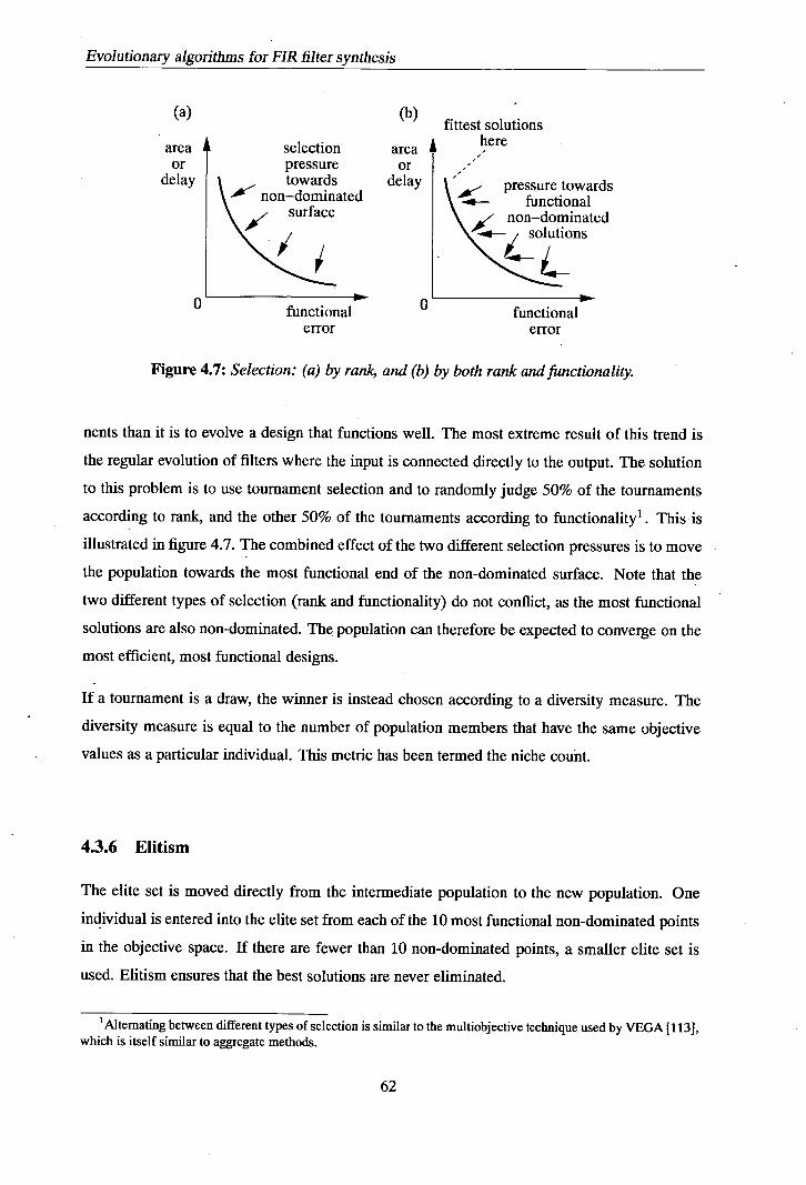
Evolutionary algorithms for FIR filter
(a) (b)
area selection area
or pressure or
delay towards delay non dominated
\surface
0 functional 0 error
fittest solutions here
I pressure towards -..-- functional
non—dominated solutions
functional error
Figure 4.7: Selection: (a) by ran/c, and (b) by both rank and functionality.
nents than it is to evolve a design that functions well. The most extreme result of this trend is
the regular evolution of filters where the input is connected directly to the output. The solution
to this problem is to use tournament selection and to randomly judge 50% of the tournaments
according to rank, and the other 50% of the tournaments according to functionality'. This is
illustrated in figure 4.7. The combined effect of the two different selection pressures is to move
the population towards the most functional end of the non-dominated surface. Note that the
two different types of selection (rank and functionality) do not conflict, as the most functional
solutions are also non-dominated. The population can therefore be expected to converge on the
most efficient, most functional designs.
If a tournament is a draw, the winner is instead chosen according to a diversity measure. The
diversity measure is equal to the number of population members that have the same objective
values as a particular individual. This metric has been termed the niche count.
4.3.6 Elitism
The elite set is moved directly from the intermediate population to the new population. One
individual is entered into the elite set from each of the 10 most functional non-dominated points
in the objective space. If there are fewer than 10 non-dominated points, a smaller elite set is
used. Elitism ensures that the best solutions are never eliminated.
'Alternating between different types of selection is similar to the multiobjective technique used by VEGA [113], which is itself similar to aggregate methods.
62

Evolutionary algorithms for FIR filter synthesis
module fir(in,out,clk,rSt), input clk,rst; input [7:0] in; output [15:0] out; wire [12:3] wO;
wire [18:3] w45; register_8bit fr12 (w12,clk,ifl,rSt);
register_16bit fr2l (w21,clk,w44,rst); adder 10 aO ( wO,{{2{in[7]}},ifl},{{1{irl[7]}},ifl,l'b0},l'bO)
adder 12 al (w1,{{1{in[7]}},ifl,3'b0},{{4{in[7]}},in},'bO)
adder-14 a2 (w2, {wi, 2 'bO}, {{6{in[7]}} , in}, 1 'bO); adder 12 a8 (W8,{{2{w0[12]}},W0},{W0,2'bO},i'bO)
adder-11 a36 ( w36,{{1{wO[12]}},wO},{(2{W12[7]}},W12,i'bO}ri'bO) adder 11 a37 (W37,1{2{ifl[7]11,ifl,l'b0},wl3,1'bl) adder 13 a38 (w38,{{l{w8[14]}},w8},{{2{wi4[13]}},w14}li'bl);
adder-14 a39 ( w39,{{i{w8[14]}},W8,l'bO},{{i{wi5[15]}},wiS},l'bi)
adder-15 a40 ( W4O, - {{l{W2[16]}},W2},{{1{w16[16]}},W:1.6},l'bfl adder 15 a41 (W4l,{(2{W8[14]}},W8,1'b0),wl7,l'bl);
adder-16 a42 (w42,{{4{w8[i4]}},W8},{{i{wi8[i7]}},8}fl');
adder 16 a43 (w43,{{7{in[7]}},in,i'b0},W19,i'bi)
adder _i6a44 (W44,{{6{wO[12]}},W0},W20,i'bO) adder-16 a45 (W45,{{7{in[7]}},ifl,l'b0},W21,i'b0) assign out = w45; endinodu le
Figure 4.8: An example filter netlist.
43.7 The evolutionary algorithm
The EA is a (p + A) system, where an existing population of p individuals is expanded through
the creation of A children, and the intermediate population of p + A individuals must then
compete for the p places in the new population. The advantage of a (p + A) system is that good
individuals can survive for many generations, in contrast to a (p, A) system, where the children
replace the parents every generation. The experiments in this chapter have used p = A = 100.
When expanding the population, parents are chosen at random. When reducing the population
size, the new population are chosen through the selection and elitism operations described
previously.
4.3.8 Circuit synthesis
Verilog netlists are produced for the evolved circuit designs. Each netlist contains a structural
description of a design; in other words, a netlist describes a set of high-level components, and
rev

Evolutionary algorithms for FIR filter synthesis
—16
—24
16
120
240
-i-F 296
-+ 240
-i-F 120
*16 -± 16
- ± —24
- ± —16
Note: lines represent buses, multiplications represent shifts. output
Figure 4.9: An evolved filter
the interconnections between them. An example is shown in figure 4.8. The same evolved filter,
with coefficient set, is shown in figure 4.9.
gam gain (dB) (dB)
3dB I : 30, 40, 3dB 30, 40, or 50dB or 50dB
+20dB +20dB Y pass ia - stop band - pass band
no 0 0.125 0.25 normalised 0 0.125 0.25 normalised
frequency frequency
input
*64
IIIL *8
Figure 4.10: Filter specifications.

Evolutionary algorithms for FIR filter synthesis
Setting Value
Population 100 Generations 20000 Crossover 50%
Components 10 Maximum taps 19 (10 symmetrical)
Input width 8 bit
Table 4.2: EA settings.
4.4 Experiments and results
4.4.1 Evolution of filters
Some test problems are shown in figure 4.10. These are low-pass and high-pass filter specifi-
cations, which attenuate by 30, 40 and 50dB in the stop bands. Filter designs that completely
meet these specifications have been termed 'correct'.
20
,, 15 0
Ca
0. 0
CL 10 75 (0 a) C) C)
(1) 5
0
5000 10000 15000 20000
Generation
30dB low-pass 40dB low-pass 50dB low-pass
30dB high-pass -------- - 40dB high-pass ........ 50dB high-pass
Figure 4.11: The number ofpopulations containing a correct solution, by generation.
The BA was applied to the problems in figure 4. 10, using the settings shown in table 4.2. Twenty
runs were performed on each problem. The results are shown in table 4.3 and in figure 4.11.
The EA was able to find correct solutions for all of the problems. The predicted area and delay
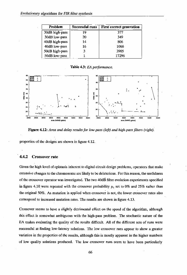
algorithms for FIR filter synthesis
Problem Successful runs I Firstcorrect generation
30dB high-pass 19 377 30dB low-pass 20 349 40dB high-pass 14 806 40dB low-pass 16 1066 50dB high-pass 3 3905 50dB low-pass 1 17296
Table 4.3: EA performance.
00dB 40d .
55 0dBB
50
45
140
135
30
25 • °.60 0
20
15 2000 2500 3000 3500 4000 4500 5000 5500 6000
area (NAND gates)
45
40
35
30
25
2020
15 2000 2500 3000 3500 4000 4500 5000 5500
area (NAND gates)
Figure 4.12: Area and delay results for low-pass (left) and high-pass filters (right).
properties of the designs are shown in figure 4.12.
4.4.2 Crossover rate
Given the high level of epistasis inherent to digital circuit design problems, operators that make
extensive changes to the chromosome are likely to be deleterious. For this reason, the usefulness
of the crossover operator was investigated. The two 40dA filter evolution experiments specified
in figure 4.10 were repeated with the crossover probability Pc set to 0% and 25% rather than
the original 50%. As mutation is applied when crossover is not, the lower crossover rates also
correspond to increased mutation rates. The results are shown in figure 4.13.
Crossover seems to have a slightly detrimental effect on the speed of the algorithm, although
this effect is somewhat ambiguous with the high-pass problem. The stochastic nature of the
LA makes evaluating the quality of the results difficult. All of the different sets of runs were
successful at finding low-latency solutions. The low crossover runs appear to show a greater
variation in the properties of the results, although this is mostly apparent in the higher numbers
of low quality solutions produced. The low crossover runs seem to have been particularly

Evolutionary algorithms for FIR ifiter synthesis
60
55
50
7 45
40
35
30
25 3000. 3500
4000 4500 5000 5500 6000
area (NAND gates)
0% crossover *
25% crossover c 50% crossover
20
15
10
I (5 5
50
45 *
40
35
30
o0 0 00
25
20 x x x x 19000
15 2500 3000 3500 4000 4500 5000 5500 6000
area (NAND gates)
0% crossover * 25% crossover o 50% crossover
: ......
20
16
F: 2
T- o o 5000 10000 15000 20001
Generation
0% crossover 25% crossover 50% crossover
0
5000 10000 15000 20000
Generation
0% crossover - 25% crossover 50% crossover
Figure 4.13: Experiments with different levels of crossover, for the 40d6 low-pass (left) and high-pass (right) problems.
67

Evolutionary algorithms for FIR filter synthesis
Problem SPW/IM Evolved Adds I Registers Adds I Registers
30dB low-pass 16 8 11 10 30dB high-pass 14 8 10 8 40dB low-pass 19 10 16 10 40dB high-pass 19 10 14 12 50dB low-pass 28 12 24 16 50dB high-pass 16 12 20 16
Table 4.4: Comparison of component counts for evolved and conventional filters.
successful at producing low-area solutions to the low-pass problem. The conclusion that can be
drawn from these results is that crossover is not essential, and that it might actually be mildly
detrimental. Alternatively, the low crossover runs might be benefiting from increased mutation
rates.
4.4.3 Comparison with other systems
In this section, the EA is compared with the results from some other systems. These results
should be interpreted with caution for two reasons. Firstly, the EA introduced in this chapter is
a multiobjective system, and as such it attempts to strike a balance between the area and latency
of a design. Minimum area or minimum delay solutions represent extreme points on such a
trade-off surface. Finding an extreme point is not just a test of an algorithm's ability to find.
near-optimal solutions, it is also a test of how thoroughly the algorithm explores the trade-off
surface. Thus, finding a minimum area or minimum delay solution is a harder problem for a
multiobjective EA. A second point is that, for reasons of comparison, this section describes
areas in terms of component counts, and delays in terms of adder delays. The results therefore
do not include any gains achieved through using a more accurate hardware model. Indeed, if
area can be saved while increasing the component count, or if the delay can be reduced while
placing more components on the longest path, then using a more accurate model would become
counterproductive. Figure 4.14 shows the modelled area plotted against the component count
for all of the circuits evolved in section 4.4.1. It can be seen that the variations between the two
models are larger than one component area. The area required for a component is not constant,
but instead depends on the type and width of the component.
The 'Fxp.Equiripple' design method of the Cadence SPW filter design system was used
68

Evolutionary algorithms for FIR filter synthesis
30
25
20 (1)
a) -a (5
15
10
5 1000
-l-4-+-+H-+ -44+
- (1114(111 4-4-
-44-4-f 11111 111(1 III
- +-HI-I-l-IIIIl 11111(1
-44441-01-Il lII44IU liii ++
- -1-441-Ill i.UhIliiIilI 11-1+
+ llIDIlhlIl• 111111111 +
I IIlllI II 1(1111111114
#414414Ilf1444f+ +4+
+ 111Ul liii IlEllIl
111111 1111 II lull +
+ -+4- -4-1441- III UI III I I
+++-*044-Il--I440-f -I- +
-if-Il--Hf -44--4++ ++ + IllIlli I 444+1+ -4-1- -4-4- -
-4111041+ +4- * +
ll__I+ + +
+4141444- +I-+
+44-Il-I-I- ++ -111-
+44-1- +1-
+f++ +
+
2000 3000 4000 5000 6000 7000 8000
area (NAND gates)
Figure 4.14: Comparison of component counts with the modelled areas.
to generate quantised equiripple coefficient sets for the filter specifications given in figure 4.10.
The iterative matching algorithm suggested by Potkonjak et al. [36] was then used to implement
the multiplication blocks for these filter designs. These designs are referred to as the SPW/IM
designs. These two sets of designs are compared in table 4.4. The implementation of the
iterative matching algorithm was not able to compute area results using the same model as the
EA, so the results are given in terms of adders and registers rather than area. The number of
registers corresponds to the filter order, so it can be seen that the coefficient sets produced by
SPW tend to have a lower order than the evolved equivalent. The evolved filters generally use
fewer adders than the SPWIIM filters. Provided that registers have a low area relative to adders,
the evolved designs will be the most area efficient. This is the case for the library components
described in table 4.1. -
The iterative matching algorithm is designed to produce area-efficient multiplication blocks,
however it does not attempt to reduce the longest path delay. When minimising the delay, there
is no reason to use a multiplication block rather than. discrete multipliers. Table 4.5 shows
the delays required by the filters previously calculated using SPW. The filters are implemented
using CSD multipliers with balanced trees of adders. The latencies are measured in terms
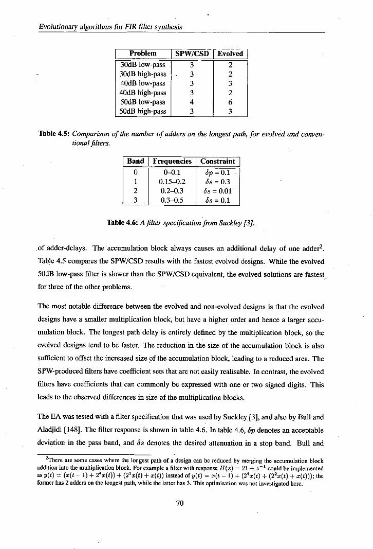
Evolutionary algorithms for FIR filter synthesis
Problem SPW/CSD I Evolved 30dB low-pass 3 2 30dB high-pass 3 2 40dB low-pass 3 3 40dB high-pass 3 2 50dB low-pass 4 6 50dB high-pass 3 3
Table 4.5: Comparison of the number of adders on the longest path, for evolved and conven-tional filters.
Band I Frequencies Constraint
0 0-0.1 6p=0.1 1 0.15-0.2 8s = 0.3 2 0.2-0.3 58 = 0.01 3 0.3-0.5 ös = 0.1
Table 4.6: A filter specification from Suckley [3]..
of adder-delays. The accumulation block always causes an additional delay of one adder 2 .
Table 4.5 compares the SPW/CSD results with the fastest evolved designs. While the evolved
50dB low-pass filter is slower than the SPW/CSD equivalent, the evolved solutions are fastest
for three of the other problems.
The most notable difference between the evolved and non-evolved designs is that the evolved
designs have a smaller multiplication block, but have a higher order and hence a larger accu-
mulation block. The longest path delay is entirely defined by the multiplication block, so the
evolved designs tend to be faster. The reduction in the size of the accumulation block is also
sufficient to offset the increased size of the accumulation block, leading to a reduced area. The
SPW-produced filters have coefficient sets that are not easily realisable. In contrast, the evolved
filters have coefficients that can commonly be expressed with one or two signed digits. This
leads to the observed differences in size of the multiplication blocks.
The EA was tested with a filter specification that was used by Suckley [3], and also by Bull and
Aladjidi [148]. The filter response is shown in table 4.6. In table 4.6, op denotes an acceptable
deviation in the pass band, and Os denotes the desired attenuation in a stop band. Bull and
2There are some cases where the longest path of a design can be reduced by merging the accumulation block addition into the multiplication block. For example a filter with response H(z) = 21 + z 1 could be implemented as y(t) = (x(t - 1) + 24x(t)) +(2 2X(t) + x(t)) instead of y(t) = x(t - 1) + (24x(t) + (22x(t) + x(t))); the former has 2 adders on the longest path, while the latter has 3. This optimisation was not investigated here.
fill

Evolutionary algorithms for FIR filter synthesis
Problem Results from [4] Evolved Adds Registers Adds I Registersj
10dB 3 2 3 2
20dB 9 8 12(11) 8
30dB 17 16 20(19) 18
Table 4.7: Comparison with results from Redmill et al. [4].
Aladjidi evolved a filter which matches this specification, and which uses 12 adders in the
multiplication block. According to the impulse response mentioned in [148], the filter requires
19 registers and a further 13 adders in the accumulation block, resulting in a total requirement
of 19 registers and 25 adders. Bull and Aladjidi used functionality as the sole objective; they did
not attempt to minimise the area or delay of their filters. Suckley mentioned an evolved solution
to this problem that uses 11 adders in a cascade filter, however the number of registers was not
documented. The best filter produced from 20 runs of the EA introduced in this chapter is a
14th order filter that requires 19 adders and 14 registers. It has a longest-path delay of 3 adders.
This filter is estimated to have an area of 4242 1um2 and a delay of 25.6ns. The multiplication
block requires 5 adders, however one of these adders performs a multiplication by 2, so the
total number of adders could be reduced to 18 through strength reduction.
A comparison with the results in [4] is shown in table 4.7. These results relate to low-pass
filters, with the pass band at 0-0.15 and the stop band at 0.25-0.5. The maximum pass band
ripple was set equal to the maximum stop band ripple (op = Os). The numbers in brackets
in table 4.7 denote cases where an adder can be removed by strength reduction. The system
developed by Redmill et al. gives results with lower component counts.
As noted above, some of the evolved designs include redundant components. One example of
this problem is the use of an adder to perform a multiplication by a power of two - in which
case the adder can be replaced with a shift (strength reduction). A second example happens
when two different componçnts always calculate the same value, in which case one of the two
components can be eliminated. In both of these cases it is trivial to eliminate the redundant
components. This could be done by an extra operator which is either applied during evolution,
or else applied to the final population.
71

Evolutionary algorithms for FIR filter synthesis
4.5 Summary
This chapter has described an evolutionary algorithm for designing linear-phase multiplierless
FIR filters. The filters are designed with respect to a frequency domain specification. Circuit
area and longest path latency are also minimisation objectives for the BA. The EA produces a
set of solutions, and in most cases there are multiple non-dominated solutions. In some of the
examples it was seen that the trade-off surface can account for as much of 20% of the absolute
area and delay values.
The area and delay values are modelled using values derived from actual arithmetic compo-
nents. The current netlists use unlimited precision for calculations, and as a result, the compo-
nent widths were often found to vary by more than a factor of two in a single circuit. For this
reason, the hardware models take account of variations in component width.
The EA sometimes produces multiplication blocks that contain some redundant hardware. One
possibility is the inefficient use of an adder to multiply a value by 2. A second possibility is the
recalculation of the same sum by two different adders. These inefficiencies only seem to affect
a minority of circuits, nonetheless they are undesirable. Their continued selection suggests that
the EA is not always capable of eliminating the inefficiency. One possibility is to explicitly
identify and correct such circuits, either during or after evolution.
The usefulness of the crossover operator was investigated. It was found that crossover can be
disabled without compromising the speed of the EA or the quality of the results.
The BA can compete with a conventional system based upon calculating a coefficient set, and
then synthesising a filter using either iterative matching or CSD multipliers. In terms of com-
ponent counts, it was found to give results superior to the results in [148], but inferior to the
results in [4].
In conclusion, this chapter has described a multiobjective EA for the evolution of efficient
multiplierless filter hardware designs. The BA makes use of realistic area and delay models
in order to evolve hardware that is targeted at a particular technology. This chapter is also a
first step in investigating the more general problem of evolving high-level signal processing
hardware using a graph chromosome that directly represents the structure of the circuit.
72

Chapter 5 The evolution of sequential circuits
5.1 Introduction
This chapter investigates the evolution of a class of sequential circuits. These sequential circuits
perform a single computation over two or more cycles. While the circuits evolved in chapter 4
could be considered sequential due to the inclusion of registers, they only had one state of
operation and performed the same task in every cycle. The circuits evolved in this chapter
are controlled by state machines (albeit simple ones), and go through several states in order to
perform a single computation.
There are several existing systems that perform scheduling using an EA [163-167].. These
systems perform scheduling, allocation and binding for all operations in a data-flow graph
(DFG). They take a DFG as input and produce a sequential circuit design as output. EAs have
also been used for pipelining data-flow graphs [121], again starting with a functionally correct
DFG. In contrast, the system introduced in this chapter performs scheduling in parallel with
evolution of the functionality of the circuit.
There are two objectives to the work in this chapter. The first, more minor objective is to demon-
strate a technique that can reduce the area required for a particular task. The major objective is
to demonstrate the evolutionary design of some members of a useful class of sequential circuits.
It is hoped that the techniques introduced in this chapter will enable the evolution of circuits
that can only be practically realised using sequential hardware.
This chapter builds upon the software developed in chapter 4.
5.2 Multistate sequential circuits
This chapter investigates circuits that perform one computation over a set number of cycles.
These circuits are controlled by a state machine such as those shown in figure 5.1. An n-state
circuit can process one set of data every n cycles. The circuits can contain multiplexors that
73

The evolution of sequential circuits -
state
state 0 state
state
Figure 5.1: 2-state and n-state state machines.
are controlled by the state machine, and which enable the reconfiguration of the datapath every
cycle. Ideally, the area requirement of an n-state sequential circuit could approach 1/n of the
area of an equivalent combinatorial circuit, however the savings are limited by the need for
extra registers and multiplexors.
In this chapter, the EA system introduced in the previous chapter is modified so that the mul-
tiplication block operates sequentially. The multiplication block therefore uses a faster clock
speed than the accumulation block. The initial investigation focuses on the development of
2-state multiplication blocks, but n-state multiplication blocks are investigated later.
5.3 2-state hardware
input
output
state
Figure 5.2: A 21-times multiplier using two additions, performed using one adder, two MUXs and one register.
The datapath for a 2-state multiplication block differs from combinatorial designs in two ways.
Firstly, each component input can connect to a different location in each state, in which case
a multiplexor is necessary. A multiplexor is also necessary if an input requires different shifts
74

The evolution of sequential circuits
in different cycles. Common subexpression elimination can prevent the creation of multiple
identically configured multiplexors. Secondly, a register is required whenever a value that is
produced in cycle 0 is used in cycle 1. It should be emphasised that the requirement for registers
and multiplexors varies from circuit to circuit, and that better designs use few such components.
An example is shown in figure 5.2.
5.4 Modifications to the EA
operations taps
The packedop op op op op op tap tap tap chromosome: 1 2 3 4 1 5 6 1 1 2 3
rip op op 3 5
op op op tap tap tap 2 4 6 123
cycle 0:
cycle 1:
Adder 1 Adder 2 Adder 3
Figure 5.3: How the position of an operation within the chromosome is used to encode schedul-ing and binding information.
The EA used in this chapter is a modified version of the EA introduced in chapter 4. The
following changes were performed to enable the evolution of multistate hardware.
• The chromosome was changed to include scheduling and binding information.
• An extra evolutionary operator, which modifies the scheduling information, was intro-
duced.
• The functions that perform hardware modelling and netlist generation were updated to
reflect the nature of the hardware being generated.
When designing a combinatorial circuit, there is a one-to-one correspondence between com-
ponents and operations. With sequential hardware, each component can perform a different
operation in each cycle. The chromosome can either represent a dataflow graph (DFG), or else
it can directly represent a circuit. If the chromosome represents a dataflow graph, the genes
represent operations, and the chromosome must also include some scheduling and binding in-
formation. It should then be relatively easy to modify the scheduling and binding of individual
75

The evolution of sequential circuits
operations. If the chromosome directly represents a sequential circuit, the genes describe com-
ponents. The schedule is then implicitly coded through the explicit use of components such as
multiplexors. The problem with a component-based strategy is that changes to the chromosome
have effects in every cycle, so the search landscape will be extremely multimodal. Therefore,
a DFG-based strategy was chosen. The scheduling and binding information for each operation
was encoded by the position of the operation within the chromosome. Odd-numbered oper-
ations are performed in cycle 0, and even-numbered operations are performed in cycle 1, as
shown in figure 5.3.
The interpretation of the genes that represent connections was altered, so that operations cannot
depend on future results. Inputs that depend upon future values are remapped to the past or
present, using the modulus operation. The inputs for all operations in cycle c are interpreted as
originating in a cycle modulo c + 1.
In order to allow the rescheduling of the operations in a chromosome, the 'swap operations'
mutation operator was introduced. This randomly chooses two operations within a chromo-
some, and swaps their positions, causing the scheduling and binding of the operations to also
be swapped. The 'swap operations' operator will also change other genes within the chro-
mosome, so that connections are not broken and the functionality of the circuit is unchanged.
However, if an operation is moved to an earlier time-slot, data dependencies might still lead to
a change in circuit functionality. The complete list of mutation operations is now as follows:
• Conventional mutation.
• Scale value.
• Insert component.
• Remove component.
• Duplicate component.
• Swap inputs.
• Swap operations.
When a mutation is applied, a single operator is chosen at random from the above list. As
before, crossover is applied in 50% of cases, and mutation is applied in the other 50% of cases.
76

The evolution of sequential circuits
Component Area Delay (NAND gates) (nanoseconds)
16-bit adder 196.85 10.77 16-bit register 85.28 -
16-bit 2-1 MUX 37.28 7.59
Table 5.1: Component properties.
Law-pm results
60 50
45
40
35
o 30
25
20
'5
• 2000 2500 3000 3500 4000 4500 5000 5500 6000
area (NANO gates)
I-Ugh-pass results
60
70
60
50
a 40
30
20
2500 3000 3500 4000 4500 5000 5500 6000 6500 7000
area (NAND gates)
Figure 5.4: Correct results for the test problems.
Assessment of functionality is unchanged from the previous chapter, with the addition of the
causality constraints mentioned above. Unlike the system introduced in the previous chapter,
all components are the same width. This simplifies modelling and netlist generation. The
hardware modelling system first calculates where registers and multiplexors are needed. The
delay model must consider both adders and multiplexors as sources of delay. The longest-
path delay is calculated for each cycle independently, and the largest delay value defines the
longest path delay for the whole circuit. The area model now reflects the fact that registers and
multiplexors are used in the multiplication block. The component properties are derived from
the same 0.35um library as used in chapter 4— they are shown in table 5.1.
5.5 Results
The modified EA was tested on the problems that were previously introduced in figure 4.10.
It produced correct results for all of the problems except for the 50dB low-pass problem. The
properties of the results are shown in figure 5.4. Note that the longest path delay refers to the
time for a single cycle, so twice that time is needed to process a data item.
77
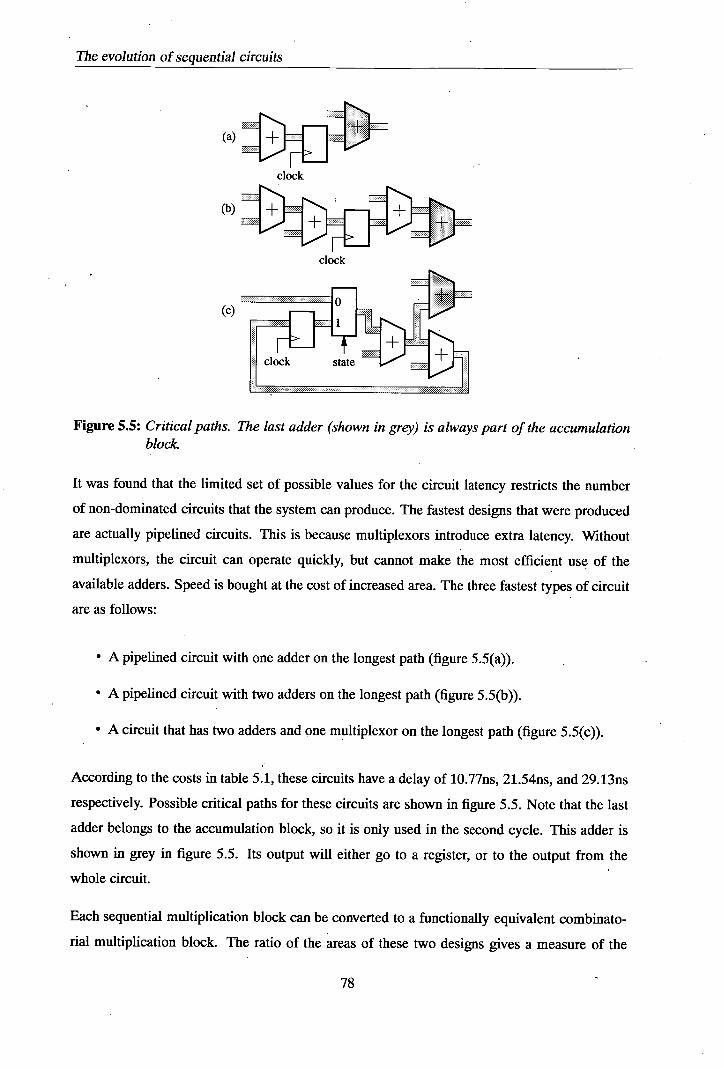
The evolution of sequential circuits
clock
(b)
clock
(c)
Figure 5.5: Critical paths. The last adder (shown in grey) is always part of the accumulation block
It was found that the limited set of possible values for the circuit latency restricts the number
of non-dominated circuits that the system can produce. The fastest designs that were produced
are actually pipelined circuits. This is because multiplexors introduce extra latency. Without
multiplexors, the circuit can operate quickly, but cannot make the most efficient use of the
available adders. Speed is bought at the cost of increased area. The thee fastest types of circuit
are as follows:
• A pipelined circuit with one adder on the longest path (figure 5.5(a)).
• A pipelined circuit with two adders on the longest path (figure 5.5(b)).
• A circuit that has two adders and one multiplexor on the longest path (figure 5.5(c)).
According to the costs in table 5.1, these circuits have a delay of 10.77ns, 21.54ns, and 29.13ns
respectively. Possible critical paths for these circuits are shown in figure 5.5. Note that the last
adder belongs to the accumulation block, so it is only used in the second cycle. This adder is
shown in grey in figure 5.5. Its output will either go to a register, or to the output from the
whole circuit.
Each sequential multiplication block can be converted to a functionally equivalent combinato-
rial multiplication block. The ratio of the areas of these two designs gives a measure of the
in

The evolution of sequential circuits
Low-pass area savings I-Ugh-pass area savings
1800
1600
l400
1200
i l000 800
0)
600
don 400 600 500 1000 1200 1400 1600 1800
Combinatorial area (NAND gates)
no saving - 20% saving 30dB 10% saving --- 30% saving 40dB
2000
1800
1600
1400
1200
1000
800
600
400
20 200 400 600 800 1000 1200 1400 1600 1800 2000
Combinatorial arm (NAND gates)
no saving - 30% saving - 50dB 10% saving ------ 30dB 2(Y% saving ---------- -40dB
Figure 5.6: Comparison of sequential and equivalent combinatorial areas for evolved multi-
plication blocks.
Low-pass area savings High-pass arm savings
6500
6000
- 5500
5000
4500
4000
! 3500
3000
° 2500
2000
150 2500 3000 3500 4000 4500 5000 5500 6000 6500
Combinatorial area (NAND gates)
no saving 2D% saving 30dB * 10% saving -- 30% saving 40dB
8000
7000
6000
5000
8 4000
3000
2000
1000 jsoo 3000 3500 4000 4500 5000 5500 60M ssao moo moo
Combinatorial area (NAND gates)
no saving 30% saving 50dB 10% saving - 30dB 20% saving ---------- 40dB -
Figure 5.7: Comparison of sequential and equivalent combinatorial areas for evolved filters.
79

The evolution of sec,uential circuits
Problem. SPWJIM original EA multistate EA Adds Registers Adds] Registers Adds Registers MUXs
30dB low-pass 16 8 11 10 8 9 4 30dB high-pass 14 8 10 8 8 10 3 40dB low-pass 19 10 16 10 13 15 4 40dB high-pass 19 10 14 12 13 14 2 50dB low-pass 28 12 24 .16 - - - 50dB high-pass 16 12 20 16. 18 19 6
Table 5.2: Component counts for three different filter implementation techniques.
Scheme I Adders I Registers I MUXs I Conventional n I I 0
2-state n 2
3n I + 1 + 1
Table 5.3: Components required for an n-th order accumulation block
area saving that is achieved through the use of the sequential design. The combinational and
sequential areas of the multiplication blocks from the correct designs are plotted in figure 5.6.
In the best case, using the sequential scheme leads to an area saving of 28%. This figure relates
to the multiplication block alone. When the area of the accumulation block is also included, the
area savings are smaller, as shown in figure 5.7. This is because the area of the accumulation
block is the major part of the area of a design, and it has the same area in both cases. The
design for a multistate accumulation block will be described in section 5.6. When the area of
the accumulation block is included, the best saving is about 7%. In some cases, the sequential
designs have a greater area than the combinatorial equivalent - although, as noted above, this
can be due to the evolution of pipelined designs.
In the table 5.2, the results from table 4.4 are extended to include the component counts for
the multistate system. The results show that the multistate EA requires lower numbers of
adders than the original EA, but increased numbers of registers and multiplexors. The non-
evolutionary system is superior to either EA for the 50dB high-pass problem, but requires
larger numbers of adders in other cases. If the component properties from table 5.1 are used,
the multistate EA gives the smallest results for both 30dB problems and for the 40dB low-pass
problem.
Kc

The evolution of sequential circuits
output
.te
input input input input input 0 3 1 4 2
Note: Clock speed is twice data rate. Inputs are valid in state 1. Output is valid in state 0.
Figure 5.8: A 2-state accumulation block
5.6 A multistate accumulation block
The EA system described in this chapter uses a conventional accumulation block, however a 2-
state accumulation block could be used instead. A multistate architecture for the accumulation
block is shown in figure 5.8. The costs of these two schemes are compared in table 5.3. When
using the properties in table 5.1, the 2-state accumulation block makes a 13% area saving,
assuming m is large. The 2-state scheme introduces an extra multiplexor delay onto the longest-
path of the accumulation block.
5.7 Operation over many cycles
The system for creating 2-cycle sequential circuits was extended, so that circuits that operate
over many cycles could be created. The number of cycles that the design should use could be
defined at the start of evolution.
The calculation of area and delay information becomes much more complicated in the multi-
cycle case. This is because the most efficient way of organising the registers and multiplexors
is no longer obvious. A poor-quality solution to these problems was simply to ignore the extra
area and latency introduced by the registers and multiplexors, and only to take account of the
adders in the circuit. This reduced the complexity of the circuit modelling system, but also
01

The evolution of sequential circuits
prevented accurate computation of the circuit area and delay. Circuit netlists could no longer
be generated.
When evolving filters that operate over three or more cycles, it was found that the system
would often create inefficient designs. This is because the number of available operations is
often poorly matched to the number of required operations. This, combined with the extra area
that will be needed for registers and multiplexors, leads to a very low benefit, when applied to
the FIR POF circuit creation problem. As an example of this problem, consider the scheduling
of four additions over two cycles, and, also over three cycles. In the 2-cycle case, two adders
are used, and each adder performs two additions. In the 3-cycle case, two adders must still be
used, but only four of the six available additions are needed. This means that the 3-cycle case is
no more efficient than the 2-cycle case. In fact, the 3-cycle case might be less efficient, as more
area could be dedicated to registers and multiplexors. This inefficiency is most notable when
there are few components. As the number of cycles is increased there will be a point where
it becomes most efficient to use a general purpose circuit, composed of a register file and an
arithmetic unit.
5.8 Application to other problems
Other types of sequential circuit can be evolved using similar techniques. The main require-
ments are that the problem should be amenable to the evolution of solutions, and the compu-
tational components should have a large area relative to registers and multiplexors. Problems
that require larger numbers of operations could be suitable for implementation with hardware
that runs over more than 2 cycles.
5.9 Summary
This chapter has demonstrated an EA system that evolves sequential circuits. The EA cre-
ates a fuhctionally correct design, while simultaneously scheduling and binding the individual
operations performed by the design. The EA evolves FIR filters that use sequential multipli-
cation blocks. The filters were evolved according to a frequency-domain specification, with
multiplication blocks that operate over 2 cycles. When compared with equivalent combinato-
rial designs, multiplication block area savings of up to 28% were demonstrated. The large size

The evolution of sequential circuits
of the accumulation block limits the effectiveness of reducing the multiplication block area -
use of the 2-state multiplication blocks led to best-case filter area savings of about 7%. For this
reason, a 2-state accumulation block was investigated, with expected area savings of up to 13%.
Other types of sequential circuit could also be evolved, using similar methods. Multistate cir-
cuit implementations are most useful when computational components are expensive in terms
of area, and when registers and multiplexors are relatively cheap. The requirement for an accu-
mulation block, and the consequent limitation of the area saving, is peculiar to the multiplierless
FIR filter design problem.
The evolution of circuits that operate over more than two cycles was investigated. It was noted
that the circuits are most efficient when the number of operations is a multiple of the number
of states, and that this becomes less likely as the number of states is increased. The problem
of creating efficient multistate storage and switching networks is complex, and has not been
addressed in this thesis.
83
Chapter 6 The evolution of multiplierless linear
circuits
6.1 Introduction
This chapter introduces an evolutionary algorithm for the implementation of multiplierless lin-
ear transforms. The evolved circuit designs can have multiple inputs and multiple outputs. Each
circuit design can be characterised by a transformation matrix.
Linear transforms are used as a building block for an enormous variety of signal processing
applications. This includes practical applications in areas such as data compression, signal
conditioning, and signal analysis. A particular advantage of linear systems is the ease with
which they can be characterised, which is something that is also useful in the context of this
chapter.
While the work in this chapter was inspired by the work in chapter 4, the EA is a completely
new implementation.
6.2 Problem statement
A linear transform can be specified as follows:
y=Hx (6.1)
where x and y are column vectors containing the N inputs and M outputs, and where H is an
(M x N) matrix of coefficients. If H is unknown, it can be found by applying a series of inputs
Xl, , XM, such that element n of Xn is one, and all other elements are zero. The outputs then
correspond to the columns of H.
The problem of implementing a linear transform can be stated as follows. Given a user-supplied
ideal response matrix H2 , construct a linear transform circuit with the actual response matrix

The evolution of multiplierless linear circuits
Ha, such that Ha H2 . The circuit should be as efficient as possible. In this chapter efficiency
is defined as low area consumption and a short longest path delay.
6.3 The evolution of linear transforms
63.1 The chromosome
Figure 6.1: A chromosome and the corresponding circuit design.
A graph chromosome has been used. Each node in the graph represents an addition. Each node
has two inputs. The inputs to a node can be negated and shifted. Depending on which inputs
are negated, the node can correspond to one of the following implementations:
an adder,
a subtracter,
an adder followed by a negator.

The evolution of multiplierless linear circuits
The inputs to a node can connect to any circuit input or node output. The circuit outputs can be
shifted, and negators can be inserted at the circuit outputs. In other words, a node can calculate
a value +28u + 2tv , where u, v are the node inputs and s, t e Z select how many bit-positions
the input values should be shifted. A circuit output can take values of the form ±28u, where u
is the value at a node or input and s is the shift.
Figure 6.1 shows an example chromosome and the corresponding circuit design. This repre-
sentation is more flexible than the linear representation introduced in figure 4.4. The graph
representation introduced here can encode subtractions and negations, and represent designs
which have multiple inputs and multiple outputs.
A cyclic graph corresponds to a circuit that contains an unclocked feedback loop, which is
undesirable. If a chromosome is found to contain a cycle, the chromosome is replaced with a
trivial design that is guaranteed to be acyclic. In this way the population is kept acyclic.
6.3.2 Initial population
The initial population contains designs where each output is directly connected to a randomly
selected input. No shifts or negations are used. The designs in the initial population therefore
have no area and no delay.
6.3.3 Evolutionary operators
There is no crossover operator. The chromosomes are modified by the following mutation
operators:
Change connection - reconnect a node input to a different source.
Insert node - insert a new node, which adds a randomly selected value to a pre-existing edge.
Change shift - change the shift and negation at a node input or an output. The shift is in-
cremented or decremented. lithe shift is at the minimum allowable value, the edge is
instead negated.
Associativity - swap the positions of two connected nodes; for example replacing (a + b) + c
with a+(b+c).
87

The evolution of multiplierless linear circuits
Delete node - a node is chosen at random and eliminated. The source, shift and negation
information from one of the node inputs is propagated to the input of all of the nodes that
depend upon the eliminated node.
The 'change connection' and 'insert node' operators form new edges. When forming a new
edge, these operators must decide how much shift should be applied. If too great a left-shift
is used, it can easily introduce a large error into the response of the circuit. If the shift results
in a value that is too small, the value at the node will be defined by the other input, and the
node will be redundant. It is also worth noting that large shifts are sometimes useful, so it is
sometimes helpful if they can be created. As a compromise between these conflicting effects,
new connections are randomly assigned a shift of up to +4 bits. Increasing this range causes the
algorithm to run slower, while reducing this range increases the area and delay of the evolved
designs. New connections are negated with probability 50%.
If an evolutionary operator causes some nodes to become redundant, then those nodes are elim-
inated from the chromosome. The chromosome only contains nodes that connect to the outputs,
either directly or indirectly.
6.3.4 Fixed-point and integer operation
The EA has two modes of operation, fixed-point mode and integer mode. In integer mode
right-shifts are disabled, and the EA can only create designs that use integer coefficients. In
fixed-point mode the EA can produce both left- and right-shifts, so the EA can design hardware
with fractional coefficients.
In integer mode, left-shifts that are common to both node inputs are eliminated. This is achieved
by repeatedly using the rule of distributivity and replacing a shift that is common to both com-
ponent inputs with a shift at the component output. In other words, the value computed at a
node is altered as follows:
(a << si) + (b << (si + 82)) =. (a + (b << s2)) << S1
where a and b are the node input values, s1 is the common left-shift and s2 is the left-shift that
is not common to both inputs. While applying this transformation does not change the func-
tionality of a design, it does make the intermediate values smaller. Without this transformation,
0.

The evolution of multiplierless linear circuits
it was found that the EA was unlikely to correct a chromosome that has only a small functional
error.
In fixed-point mode, the fractional coefficients can cause the functional error to also become
fractional. The functional error typically reduces asymptotically towards zero as evolution
progresses. If this trend is allowed to continue unrestricted, it results in circuit designs that
include a large number of components, and which have a functional error that is extremely close
to zero. These circuits are probably too expensive in terms of area and delay, so it is important
to constrain the growth of the designs. This is done by letting the user specify an acceptable
functional error. This is a level of error below which designs are considered functionally correct.
Functionally correct designs can only compete in terms of area and delay, so they do not become
bloated.
6.3.5 Assessment of functionality
The user supplies the desired transformation matrix, which is known as the ideal matrix H2 . The
response of a circuit is found by setting each input to i in turn, while the other inputs are set to
0. The circuit's actual response matrix, Ha, can then be constructed from the circuit outputs.
The response matrix is subtracted from the ideal matrix, giving an error matrix He = Ha - H.
The functional error of a circuit is defined as the sum of the squares of all of the elements in the
error matrix. Functionality is a minimisation objective; better circuits have a lower functional
error.
As mentioned previously, it is useful for the user to be able to specify a level of error that
is considered acceptable. If the user specifies an acceptable error, all functional error values
are made greater than or equal to this level, so all functionally acceptable chromosomes are
considered equivalent.
6.3.6 Hardware modelling
The EA has the ability to produce three distinct types of design:
• Fixed-width bit-parallel designs.
• Variable-width bit-parallel designs.
Me
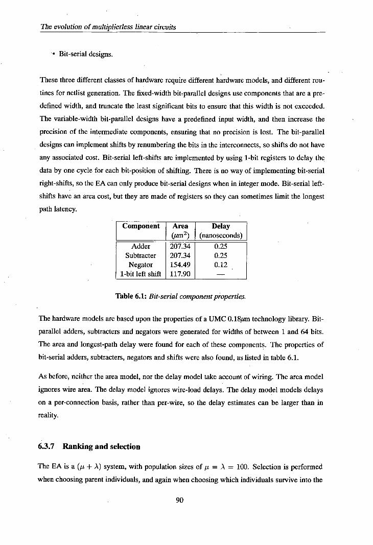
The evolution of multiplierless linear circuits
• Bit-serial designs.
These three different classes of hardware require different hardware models, and different rou-
tines for netlist generation. The fixed-width bit-parallel designs use components that are a pre-
defined width, and truncate the least significant bits to ensure that this width is not exceeded.
The variable-width bit-parallel designs have a predefined input width, and then increase the
precision of the intermediate components, ensuring that no precision is lost. The bit-parallel
designs can implement shifts by renumbering the bits in the interconnects, so shifts do not have
any associated cost. Bit-serial left-shifts are implemented by using 1-bit registers to delay the
data by one cycle for each bit-position of shifting. There is no way of implementing bit-serial
right-shifts, so the EA can only produce bit-serial designs when in integer mode. Bit-serial left-
shifts have an area cost, but they are made of registers so they can sometimes limit the longest
path latency.
Component Area Delay (um') (nanoseconds)
Adder 207.34 0.25 Subtracter 207.34 0.25 Negator 154.49 0.12
1-bit left shift 117.90 -
Table 6.1: Bit-serial component properties.
The hardware models are based upon the properties of a UMC 0. 18gm technology library. Bit-
parallel adders, subtracters and negators were generated for widths of between 1 and 64 bits.
The area and longest-path delay were found for each of these components. The properties of
bit-serial adders, subtracters, negators and shifts were also found, as listed in table 6.1.
As before, neither the area model, nor the delay model take account of wiring. The area model
ignores wire area. The delay model ignores wire-load delays. The delay model models delays
on a per-connection basis, rather than per-wire, so the delay estimates can be larger than in
reality.
6.3.7 Ranking and selection
The EA is a (t + A) system, with population sizes of It = A = 100. Selection is performed
when choosing parent individuals, and again when choosing which individuals survive into the
90

The evolution of multiplierless linear circuits
next generation.
The population is ranked using the non-dominated sorting algorithm. Size-2 tournament se-
lection is used. 50% of the tournaments are judged by rank, and the other 50% are judged by
functionality. This encourages the discovery of solutions that are both functional and efficient.
In the event of a tournament being judged a draw, the winner is the individual with the lowest
niche count. The niche count is equal to the number of individuals that have identical objective
values.
An elite set is preserved when the population size is reduced. The elite consists of one individual
chosen from each of the 10 most functional non-dominated points. If there are fewer than 10
non-dominated points, a correspondingly smaller elite set is used.
6.4 Experiments
6.4.1 Test problems
Four test problems have been used in this chapter. They are the 4-point DCT, the 8-point DCT,
the RGB to XYZ colour transform, and the 8-point Discrete Hartley Transform (DHT). The
DCT was introduced in chapter 2, and the other two problems are introduced here. Most of the
EA runs were performed in integer mode, in which case the coefficients were scaled up and
rounded to integer values. The matrices for the test problems are listed in appendix B.
When processing colour images, the transformation from an RGB colour representation to an
XYZ colour representation can be specified as follows [13]:
X 0.49 0.31 0.20 R
Y = 0.17697 0.81240 0.01063 G (6.2)
Z 0.00 0.01 0.99 B
The Discrete Hartley Transform (DHT) is related to the Fourier transform and the Cosine trans-
form. The DHT can be computed using only real numbers. The N-point DHT can be specified
as follows: N-i 27r1k 27r1k
y(1) = x(k) cos —k- + sin --, where 0 <1 <N (6.3)
k=O
The inverse DHT is equivalent to the DHT, but scaled by a factor of 11N. Alternatively, a
91

The evolution of multiplierless linear circuits
Problem I Correct runs I First correct generation DCT-4 14 1132
RGB-XYZ 7 3257 DHT-8 9 14337 DCT-8 2 34394
Table 6.2: Functionality results from the test problems.
factor of 11s/N can be introduced into the right-hand side of equation 6.3, making the DHT
and inverse DHT identical.
The EA was applied to each of the four test problems. 20 runs were performed on each prob-
lem. The EA was allowed to run for 5000 generations with the 4-point DCT problem, 10,000
generations with the RGB-to-XYZ problem, and 40,000 generations with the 8-point DCT and
DHT problems. The bit-parallel variable-width hardware model was used in integer mode. A
solution with a functional error of zero is considered to be 'correct'.
6.4.2 Solution functionality
le+06
100000
10000
1000
0
ts 100
LL.
10
1
0.1 L
0
5000 10000 15000 20000 25000 30000 35000 40000
Generations
Figure 6.2: The functional fitness of the best DHT design, for 20 runs.
Figure 6.2 shows the functionality score for the best solution in each population, for 20 runs
92

The evolution of m ultiplierless linear circuits
with the DHT problem, according to generation. In the beginning, there is an almost exponen-
tial decline in the functional error. The progress slows down in later generations, and a large
amount of time is spent removing the final few imperfections in the functionality of the designs.
This trend is most pronounced with the hardest problems. Note that there is a large variability
in the number of generations until a correct solution is discovered. For the DHT problem, the
fastest nm produced correct solution after 14337 generations, whereas some of the runs did not
produce any correct solutions after 40000 generations. Table 6.2 lists the details for all four test
problems.
6.4.3 Solution quality and diversity
I I I I
' 0
+ M
U
+ W
++
+4 il
h +
• +4f
+
4-point OCT + A BtoXYZ 8-point DHT *
I
I 8-point DCT
0 20000 40000 60000 80000 100000 120000 140000 160000
Area (square microns)
Figure 6.3: Properties of the evolved circuits for the test problems.
The area and delay properties of the correct solutions to the four test problems are shown in
figure 6.3. In all four cases, the size of the tradq-off surface is so small that it is insignificant.
This suggests that the area and delay objectives do not conflict. Figure 6.4 illustrates one
situation in which a conflict does arise, so the objectives are not necessarily non-conflicting,
however such conflicts do not appear to happen in practice.
The results for the DHT problem are very widely distributed in terms of area. The largest
solutions are approximately three times the size of the smallest solutions. The DHT solutions
93
20
18
16
14
12 Cl) C
ip 10
C)
8
6
4
2
n

The evolution of multiplierless linear circuits
appear in small clusters, and it was found that each cluster corresponds to the results from an
individual run.
abed a c
Figure 6.4: Minimum area and minimum delay circuits for computing f = a + b + c + d and g= b+c+d.
6.4.4 Hardware implementation styles
25
20
15 (1) C
>., a) a)
10
5
1.1
bit-paralll variable idth + ' I
bit-parallel fixed width x
bit-serial X
X
X X X
X x X
X XX( XXXX X X X • • XX X
+ )*( X X +
+ +
+ +_ +
' f+
+f
+
4, I I I
0 10000 20000 30000 40000 50000 60000 70000
Area (square microns)
Figure 6.5: Properties of 4-point DCT designs evolved with 3 different hardware models.
Figure 6.5 shows the area and delay properties of evolved 4-point DCT circuits, evolved for
the three different styles of hardware. In this case, the variable-width bit-parallel solutions
are smaller and faster, however the fixed-width bit-parallel solutions could be more efficient in
94

The evolution of multiplierless linear circuits
other situations. The longest path delay for a bit-serial design defines the time taken to process
a bit, rather than the time taken to process a sample, so the bit-serial solutions are actually much
slower than the bit-parallel equivalents.
6.4.5 Fixed-point values
100000
10000
1000
100
10
.2 1 C)
LL 0.1
0.01
0.001
0.0001
le-05 L
0 500 1000 1500 2000 2500 3000 3500 4000 4500 5000 Generations
Figure 6.6: Functional fitness in integer mode (upper lines) and fixed-point mode (lower lines).
In order to test the generation of fixed-point solutions, fixed-point solutions to the 4-point DCT
problem were evolved. The acceptable error level in the fixed-point system was set to 0.000764.
This value was chosen so that the error in an acceptable fixed-point solution is proportionate to
the rounding error in the integer coefficient set. Note however, that the fixed-point coefficients
were not scaled up, so the error values are correspondingly smaller. Figure 6.6 shows the
functional fitnesses of the populations during evolution. The initial performance of the two
different modes is similar, however integer mode becomes slower later on. While most of the
integer runs eventually achieve a functional error of zero, the fixed-point runs rapidly decline to
the acceptable level and then remain in the acceptable range. All of the fixed point runs were in
the acceptable range by generation 2500, whereas 6 of the 20 integer runs failed to find correct
solutions. It seems that the EA is not able to promptly correct small functional errors when in
integer mode, leading to the observed performance difference between the two modes.
95

The evolution of multiplierless linear circuits
0 5000 10000 15000 20000 25000 30000 0 0.5 1 1.5 2 2.5 3 3.5 4 4.5 5 Design Compiler area (square mimons) Design Compiler delay )nn)
(a) The area model compared with Design Compiler. (b) The delay model compared with Design Compiler.
Figure 6.7: A comparison of the hardware models with Synopsys Design Compiler.
6.4.6 Hardware modelling
The area and delay figures calculated by the EA were compared with the corresponding figures
calculated by Synopsys Design Compiler. Figure 6.7 shows the results of the comparison, for,
evolved variable-width bit-parallel solutions to the 4-point DCT problem. Figure 6.7 shows that
the area model produces results which are very similar to the Synopsys figures. Note that the
0. 181um technology library does not include wire area information, so both the EA area model
and the Synopsys area model do not take account of the wire area. The delay comparison
in figure 6.7(b) shows that the EA delay model is very inaccurate. The EA delay figures are
approximately a factor of 2 larger than the corresponding Synopsys figures. The delay model is
used when ranking solutions, so incorrect scaling of the results is ignored, however figure 6.7(b)
also shows that there is only a weak correlation between the two delay models. One problem is
that the delay model works with connections rather than wires, so it is too pessimistic when the
individual wires have different delays. The delay model also ignores wire-load delays, which
can have a major effect on the results.
6.4.7 Comparison with other design techniques
Table 63 compares the quality of the evolved circuits with designs produced through non-
evolutionary techniques. The comparisons are in terms of numbers of components. The compo-
nent counts in the best evolved circuits are compared with the component counts for equivalent
circuits created using the iterative matching algorithm [36]. The evolved results are competi-
tive with the non-evolved results in terms of component counts. The longest path delays of the
35000
30000
S 1 25000 S
20000
m000
10000
5000
,
14
12
10
1 8 S
4
2

The evolution of multiplierless linear circuits
Problem Area Delay IM I Evolved CSD I Evolved
DCT-4 26 17 4 4 RGB-XYZ 38 42 5 7
DHT-8 38 42 4 6 DCT-8 130 111 5 8
Table 6.3: Adder counts for evolved and non-evolved solutions to the test problems.
evolved results were compared with the longest path delay of a transform implemented using
CSD multipliers followed by a tree of adders. It was found that the evolved results are slower,
as seen in table 6.3. Note that transforms implemented using parallel CSD multipliers are fast
but very area inefficient. The CSD results therefore represent a lower bound on the delay of the
evolved designs. In chapter 7 an improved EA is developed, and results from the improved EA
are compared against the results given in table 6.3.
6.5 Summary
This chapter introduced an evolutionary algorithm for the creation of multiplierless linear trans-
form circuits. These circuits can have multiple inputs and outputs, and are specified by a user-
supplied transformation matrix. The circuit designs are evolved with the objectives of having
low area requirements and low longest path delays. The circuit area and circuit delay are mod-
elled using component properties extracted from a real 0.18um technology library. The EA can
produce bit-serial, fixed-width bit-parallel and variable-width bit-parallel designs.
The EA was found to perform faster and more reliably when right shifts could be used. This
seems to be because of difficulties when attempting to correct small functional errors using only
left shifts and integer values. Introducing right shifts corrected this deficiency.
The area and delay properties of the evolved solutions were investigated. It was found that for
each of the four problems the best solutions are clustered together in the objective space. It
was not possible to trade between area and delay for any of the result sets. This suggests that
the area and delay objectives do not conflict. While the example in figure 6.4 proves that such
conflicts can happen, they were not observed in practice.
The accuracy of the hardware models was investigated. It was found that the area model gives
97
The evolution of multiplierless linear circuits
results similar to areas calculated by Synopsys Design Compiler. The delay model was found
to be very inaccurate. This is probably due to two main factors. Firstly, the delay model does
not model wire loads, so it ignores delays introduced by excessive fanout. Secondly, delays are
modelled on a per-connection basis, which can be very inaccurate when the individual wires in
a connection have different delays.
The evolved results were found to be competitive with results from the iterative matching al-
gorithm, in terms of component counts. The evolved results were found to be slower than
high-area, low delay designs constructed from CSD multipliers and adder trees, when delay is
measured by component counts.
The EA uses a graph chromosome, and each graph directly corresponds to a circuit design.
Crossover was not used. The evolutionary operators perform simple modifications to the graph,
corresponding to actions such as splicing an adder into the circuit design.

Chapter 7 Local searches and the evolution of
linear circuits
7.1 Introduction
In this chapter, a type of local search is proposed. This local search technique is combined
with the evolutionary algorithm that was introduced in the previous chapter. The resultant
hybrid algorithm is faster than a plain EA, while still being robust enough to be used on highly
multimodal digital circuit design problems.
There are two ways in which the performance of the searching EA is improved relative to the
original EA. Firstly, the local searches reuse intermediate values between the individual circuit
evaluations, greatly reducing the computational effort required to evaluate the functionality
of an individual design. Secondly, performance was improved through the introduction of
a heuristic technique for determining where shifts and negations should occur. This greatly
reduces the effective size of the search space.
The modified EA is compared with the original EA, using the test problems introduced in
chapter 6.
7.2 Design modelling
A linear transform can be described as follows:
y=Hx (7.1)
where x is a column vector containing the N inputs, y is a column vector containing the M
outputs, and H is the (M x N) response matrix.
Figure 7.1 shows how a single connection, labelled 'X', relates to the rest of a linear system.
The relationship between the inputs and connection X can be characterised by an array of
99

Local searches and the evolution of linear circuits
innuts
a3 03
Figure 7.1: A model of how a single connection (labelled 'X') relates to the inputs and outputs of a linear system.
coefficients a = (ai, a2, ... , aN). The relationship between connection X and the outputs can
also be characterised by an array of coefficients b = (b1, b2, ... , bj4. Finally, the part of the
circuit which is completely independent • of connection X can be characterised by an (M x N)
matrix of coefficients, here called C, which is labelled as 'linear circuitry' in figure 7.1. The
response of the circuit, H, can then be restated as follows:
H=baT+C (7.2)
The method for calculating a, b, and C is described in section 7.3, below.
Note that the model shown in figure 7.1 is likely to have a completely different structure from
the design that it models. In particular, the components in the model do not correspond with
components in the actual design. The model in figure 7.1 only describes the relationships
between the inpUts, one intermediate value (at point X), and the outputs. Other details of the
design are not modelled.
If a multiplier is inserted into connection X, and the value on the connection is multiplied by
some constant k, the response of the circuit will be:
H = kbaT + C (7.3)
100
Local searches and the evolution of linear circuits
Setting k to 2, -1 or 0 enables us to model the effects of inserting an s-bit left-shift on connec-
tion X, inserting a negator, or setting connection X to zero. These three cases can be restated
as follows:
H = 2sbaT + C (7.4)
H = C_baT (7.5)
H=C (7.6)
If a value from elsewhere in the circuit (from another connection, connection Y) is added to the
value on connection X, the circuit response can be modelled as follows:
H=b(a+a')T+C (7.7)
The vector a' in equation 7.7 serves a similar purpose to a but describes the value on connection
Y rather than the original value on connection X. Combinations of the above operations can also
be described in a similar fashion.
The user-specified required response matrix, R, is now introduced. The difference between the
actual response and the ideal response-can be used to calculate an error matrix, or alternatively
•a correction matrix:
error = H - R
IM
desired correction = R - H (7.9)
The desired value, d, is the value of a which minimises the error in the response of the whole
circuit. Ideally a = d. It is not usually possible to perfectly correct the outputs by changing
the value on a single connection, however a best-case value can still be found. Connection X
does not necessarily connect to every output. For this reason, we define the set S, containing
the indices of all of the outputs that connection X does connect to:
S={xI1<s<M,bs0} (7.10)
This enables calculation of the desired value d = (d1,. .. , dN) for connection X:
d b (7.11)
SES
101
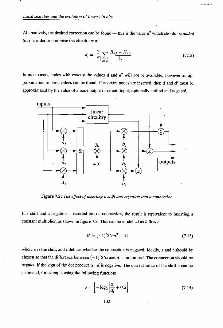
Local searches and the evolution of linear circuits
Alternatively, the desired correction can be found - this is the value d' which should be added
to a in order to minimise the circuit error.
d 1R3,—H3, - (7.12)
sES b8
In most cases, nodes with exactly the values d and d' will not be available, however an ap-
proximation to these values can be found. If no extra nodes are inserted, then d and d' must be
approximated by the value of a node output or circuit input, optionally shifted and negated.
innuts
a3 b3
Figure 7.2: The effect of inserting a shift and negation into a connection.
If a shift and a negation is inserted onto a connection, the result is equivalent to inserting a
constant multiplier, as shown in figure 7.2. This can be modelled as follows:
H = (_1)t28baT + C (7.13)
where s is the shift, and t defines whether the connection is negated. Ideally, s and t should be
chosen so that the difference between ( 1)2a and d is minimised. The connection should be
negated if the sign of the dot product a d is negative. The correct value of the shift s can be
estimated, for example using the following function:
S = [_ log2ff+o.5j (7.14)
102

Local searches and the evolution of linear circuits
This is very useful because it allows the estimation of reasonable values of the shift and negation
properties of a new connection. The overall effect is a dramatic reduction in the size of the
search space, as the EA does not need to search for good shift and negation settings.
7.3 Characterising a design
The section 7.2 made use of two matrices, H and C, as well as vectors a and b. H describes
the response of the whole design, while a, b, and C relate to a particular connection within the
design. All of these values must be calculated before the searching evolutionary operators can
proceed.
The vector a describes the response of a node in terms of the inputs. It can be found by
propagating similar vectors through the design from the inputs. The response vectors at the
inputs are trivial - for example, the first input has a response of (1,0,. . . ()) T by definition.
The response at the output of a node can be computed by scaling and summing the responses
of the node inputs.
The matrix H can be found by computing the responses of all of the circuit outputs. The
response of each output corresponds to a row in H.
The vector b describes how the outputs of a circuit relate to a particular connection. It iscalcu-
lated by transposing [11] the circuit, and then calculating the response of the same connection
in the transposed circuit, in terms of the inputs to the transposed circuit. In other words, the
vectors a and b are exchanged when a linear circuit is transposed, so the technique for finding
a can also be used to find b.
The matrix C is found by rearranging equation 7.2:
C = H_.baT
7.4 Searching evolutionary operators
Recall that the EA in chapter 6 has the following evolutionary operators:
Change connection,
(7.15)
103

Local searches and the evolution of linear circuits
• Insert node,
• Change shift,
• Associativity,
• Delete node.
The first three of these operators were changed so that they perform local searches. Before
performing the local searches, the response of the circuit is found, and the vectors a and b are
found for every node in the chromosome.
The new 'change connection' operation chooses one connection destination at random. This
can either be a node input or a circuit output. The operator then searches through all of the
possible data sources for the connection. For each possibility, the shift and negation properties
are set according to the methods described by in section 7.2 and equation 7.14. For each
possibility, the response of the system can be rapidly calculated using the following equation:
H = (_1)t28baT + C (7.16)
where the vector a' describes the relationship between the chosen data source and the circuit
inputs. The functional error can then be calculated from the circuit response in the usual way.
The connection source that results in the lowest functional error is chosen and stored.
The 'insert node' operator selects a connection at random. It inserts a new node into the con-
nection. The first input to the new node is set to the data source from the old connection, and a
search is performed in order to choose what the second input should connect to. The search is
very similar to the search performed by the 'change connection' operator. The only differences
are that the desired correction d' is used in place of the desired value d when setting the shift
and sign, and that the response of-the circuit is calculated with the following equation:
H = b(a + (_1)t2sa)T + C (7.17)
This is illustrated in figure 7.3.
The shift settings produced by both of the above operators are estimated. The 'change shift'
operator finds the completely optimal shift and negation settings using hiliclimbing. The func-
tional error is a unimodal function of the shift and negation settings, so the new settings are
104
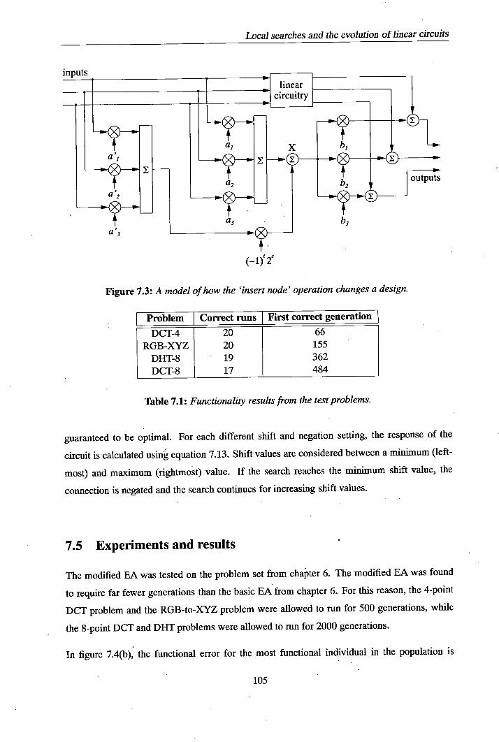
Local searches and the evolution of linear circuits
(—l) ' 2s
Figure 7.3: A model of how the 'insert node' operation changes a design.
I Problem I Correct runs I First correct generation I DCT-4 20 66
RGB-XYZ 20 155 DHT-8 19 362
DCT-.8 17 484
Table 7.1: Functionality results from the test problems.
guaranteed to be optimal. For each different shift and negation setting, the response of the
circuit is calculated using equation 7.13. Shift values are considered between a minimum (left-
most) and maximum (rightmost) value. If the search reaches the minimum shift value, the
connection is negated and the search continues for increasing shift values.
7.5 Experiments and results
The modified EA was tested on the problem set from chapter 6. The modified EA was found
to require far fewer generations than the basic EA from chapter 6. For this reason, the 4-point
DCT problem and the RGB-to-XYZ problem were allowed to run for 500 generations, while
the 8-point DCT and DHT problems were allowed to run for 2000 generations.
In figure 7.4(b); the functional error for the most functional individual in the population is
105
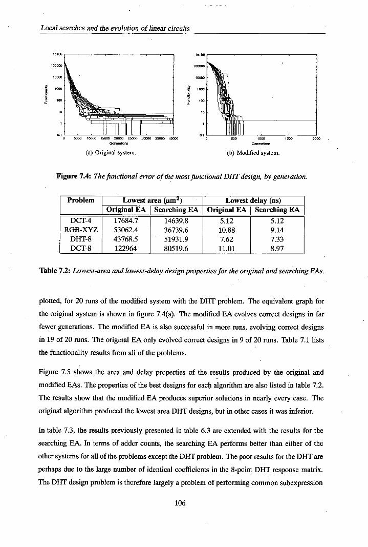
Local searches and the evolution of linear circuits
le+06
100000
10000
, 1000
100
10
0 5000 10000 15000 20000 25000 30000 35000 40000 0 500 1000 1500 2000
Generations Generations
(a) Original system. (b) Modified system.
Figure 7.4: The functional error of the most functional DHT design, by generation.
Problem Lowest area (urn 2 ) Lowest delay (ns) Original EA I Searching EA Original EA I Searching EA
DCT-4 17684.7 14639.8 5.12 5.12 RGB-XYZ 53062.4 36739.6 10.88 9.14
DHT-8 43768.5 51931.9 7.62 7.33 DCT-8 122964 80519.6 11.01 8.97
Table 7.2: Lowest-area and lowest-delay design properties for the original and searching EAs.
plotted, for 20 runs of the modified system with the DHT problem. The equivalent graph for
the original system is shown in figure 7.4(a). The modified EA evolves correct designs in far
fewer generations. The modified BA is also successful in more runs, evolving correct designs
in 19 of 20 runs. The original EA only evolved correct designs in 9 of 20 runs. Table 7.1 lists
the functionality results from all of the problems.
Figure 7.5 shows the area and delay properties of the results produced by the original and
modified EAs. The properties of the best designs for each algorithm are also listed in table 7.2.
The results show that the modified BA produces superior solutions in nearly every case. The
original algorithm produced the lowest area DHT designs, but in other cases it was inferior.
In table 7.3, the results previously presented in table 6.3 are extended with the results for the
searching BA. In terms of adder counts, the searching BA performs better than either of the
other systems for all of the problems except the DHT problem. The poor results for the DHT are
perhaps due to the large number of identical coefficients in the 8-point DI-IT response matrix.
The DHT design problem is therefore largely a problem of performing common subexpression
100000
1000C
fi000
100
10
01 -- - 0.1
106

Sc I I
S
Oriqinal ModIfied
,nnnn rrflnn coons ennon 100005 120000 140
Area (square microns)
(c) 8-point DFIT.
20
18
16
14
12 a 10
8
6
4
2
Local searches and the evolution of linear circuits
14
12
10
8
6
Orig8ral
0ModIfied
0 5000 10000 15000 20000 25000 30000 35000 40000 4500(1
Area (square microns) -
(a) 4-point DCT.
20
18
16
14 - 4 •'_&' •I
12
10
2 orilnal Modified
0 10000 20000 30000 40000 50000 60000 70000 80000
Area (square microns)
(b) RGB to XYZ transform.
16
14
12
10
a
0 - 6
Oriqinal
0 ModIfied
>00 0 20000 40000 60000 80000 100000 120000 140000 160000
Area (square microns)
(d) 8-point DCI'.
Figure 7.5: Comparison of result delay and area between the original EA system and the searching EA system.
Problem Area I Delay IM I EA I Searching EA I CSD I EA I Searching EA
DCT-4 26 17 14 4 4 4
RGB-XYZ 38 42 26 5 7 6
DHT-8 38 42 48, 4 6 6
DCT-8 130 111 69 5 8 7
Table 7.3: Adder counts for evolved and non-evolved solutions to the test problems.
107

Local searches and the evolution of linear circuits
System Problem I Generations I Time/Run (s) I Time/Generation (ii]
Original EA DCT-4 5000 93.45 18.69 Searching EA DCT-4 500 8.78 17.56 Original EA RGB-XYZ 10000 254.37 25.44
Searching EA RGB-XYZ 500 10.63 21.26 Original EA DHT-8 40000 1857.96 46.45
Searching EA DHT-8 2000 125.03 62.51 Original EA DCT-8 40000 2586.23 64.65
Searching EA DCT-8 2000 181.26 90.63
Table 7.4: Time taken for each experiment.
elimination between adder trees - a problem which the iterative matching algorithm can solve
efficiently, but which is not very amenable to iterative approximation. When delay is measured
by the number of adders on the longest path, the searching EA produces designs which are
faster than the designs from the original BA, but still slower than completely parallel CSD
implementations. The searching BA produces results that are of generally higher quality than
the results from the original BA, despite the fact that the searching EA was allowed fewer
generations.
The evolutionary operators used by the modified system require more computational effort.
This means that the number of generations is not a good indication of computational cost.
Table 7.4 lists the times taken to perform each of the different experiments'. The times were
averaged over 20 runs. Note that the size of the local search grows with the number of nodes in
the chromosome. For both EAs, the evaluation time depends on the complexity of the circuit. It
is clear that the searching BA requires far fewer generations, and that this results in much faster
run times. The local searches can cause the evaluation times to be larger for the searching BA,
but it is only a minor effect. The searching BA produces better results at a lower computational
cost.
7.6 Summary
This chapter has introduced a method for combining BAs with local searches. The hybrid
algorithm is superior to a purely evolutionary system in terms of computational requirements
and also in terms of result quality.
'Figures are for a Sun Blade 1500 workstation. Times are the 'user' times returned by the time command.
108

Local searches and the evolution of linear circuits
The technique introduced in this chapter enables the rapid functional evaluation of large num-
bers of similar designs. This means that computationally cheap local searches can be performed
by the evolutionary operators. The searching EA can evaluate the functionality of many differ -
ent designs whenever an evolutionary operator is applied. The computational cost of a single
evaluation in the local search is very low, due to the fact that many intermediate values are
common to all of the local search evaluations, so can be precomputed. The overall effect is that
the search space can be explored at a lower computational cost, when compared with a purely
evolutionary system.
This chapter introduced a method for rapidly estimating whether shifting or negation should
be applied to a connection. This eliminates a problem with the original BA, where shifts were
randomly chosen from a range of values. Previously, allowing a wide range of shift values led
to poor performance, but restricting the system to a narrow range of possible settings artificially
constrained the search space and could lead to inefficient designs. The modified BA is always
able to discover a shift setting that is close to the optimal value. This reduces the effective size
of the search space.
The technique introduced in this chapter enables the application of evolutionary algorithms to
large problems. This includes problems where evolutionary methods would previously have
been impractical.
109
Chapter 8
Local searches and the evolution of nonlinear circuits
8.1 Introduction
This chapter investigates the evolutionary design of a class of nonlinear transforms. There
are many different types of nonlinear transform, so this chapter concentrates on polynomial
transforms. A polynomial transform is a nonlinear transform where the response of each output
can be expressed as a polynomial in terms of the inputs. A polynomial transform is equivalent
to a bank of Volterra filters [19].
The EA system introduced in chapter 6 designed multiplierless linear hardware. The EA intro-
duced in this chapter implements nonlinear transforms in a similar fashion, however multipliers
must be used for the generation of the nonlinear terms in the response. Multipliers are only
used for variable-variable multiplications, and never for constant-variable multiplications. This
could be termed a 'mostly multiplierless' implementation style.
This chapter demonstrates that the local searching technique introduced in chapter 7 can be
extended to nonlinear problems.
Linear systems with variable coefficients can be specified by second order polynomials, so the
nonlinear EA - could also be useful for some linear problems. The EA system is most likely to
be useful for linear problems that require both constant and variable coefficients.
8.2 Filter specification
While chapter 2 described a matrix representation for nonlinear systems, it is inefficient for
high-order systems, where the matrices can become large and very sparse. This is a particular
concern for nonlinear systems with multiple inputs.
111

Local searches and the evolution of nonlinear circuits
The linear systems mentioned in earlier chapters can be represented as follows:
y=Hx 1991
This can be restated in a polynomial representation:
Yi h1,1 h1,2 ri;1
Y2 h2, 1 h2,2 •.. h2,N (8.2)
YM hM,1 hM,2 •.. hM,N XN
h1 , 1x1 + h1,2x2 + + hl,NXN
- h2,1x1 + h2,2x2 + ... + h2NXN
hM,lxl + hM,2x2 + ... + hM,NXN
Each output is described by a polynomial in terms of the inputs. This representation can easily
be extended to cover polynomial nonlinear systems, through the introduction of higher-order
terms. Only non-zero terms must be included, so a polynomial representation can be much
more compact than a matrix representation.
A circuit can be specified by the following information:
• The number of inputs.
• The number of outputs.
• One polynomial for each output, specifying the output in terms of the inputs.
83 The EA
8.3.1 The chromosome
The chromosome is based upon the chromosome used in chapters 6 and 7. The only difference
is that nodes can now represent multiplications, as well as additions and subtractions. This
is achieved by giving each node an extra attribute, which specifies whether the node should
perform an additive or multiplicative operation. As before, the inputs to a node can be negated,
112

Local searches and the evolution of nonlinear circuits
[Operation I Components usedi
x+y adder x - y subtracter
- (x + y) adder, negator xy multiplier
—xy multiplier, negator
Table 8.1: The mapping between graph nodes and hardware components.
resulting in the various different node implementations listed in table 8.1.
8.3.2 Initial population
The initial population is filled with randomly created chromosomes. These chromosomes have
a large number of nodes. Each connection is configured with randomly chosen source, shift and
negation properties. 10% of the nodes are multipliers, and the rest are adders and subtracters.
The connections are initialised in such a way that the initial chromosomes are always acyclic.
The chromosomes in the initial population typically have a large area and a high latency. The
average area and delay of the designs decreases rapidly in the first few generations. The designs
in the initial population are very inefficient, but their responses include many high-order terms.
This is important, as useful new terms are rarely generated later in evolution.
8.3.3 Local searches
The local searches introduced in chapter 7 were only defined for linear systems. This chap-
ter introduces local searches that can be applied to nonlinear systems. The most significant
difference between linear and nonlinear systems is that the input to a nonlinear system can-
not generally be calculated from a given output. This means that there cannot be a nonlinear
equivalent to the 'desired correction' introduced in the previous chapter. As a result, there is no
nonlinear equivalent to the technique for choosing shifts that was introduced for linear systems.
Like the local searches introduced in chapter 7, the local searches introduced in this chapter-re-
duce the computational cost of functionally evaluating a design, by sharing intermediate values
between several evaluations.
The nonlinear response is found at each node. This is a polynomial in terms of the inputs. A
single connection in the design can then be selected at random. This connection will later be
113

Local searches and the evolution of nonlinear circuits
inputs
non—linear outputs circuitry
non—linear ~20circuitry
Figure 8.1: A model of a nonlinear system, where one connection has been selected for modi-fication.
modified. The connection is then labelled as a, and treated as an unknown. The outputs are
then characterised by polynomials in terms of the inputs and the chosen connection. This is
illustrated in figure 8.1. A particular design can then be evaluated by substituting a with the
response of a node. The computational cost of a 'functional evaluation is therefore the cost of
performing these substitutions, which is lower than the cost of re-computing the response of
the whole design.
Note that figure 8.1 has some similarities with the decomposition of a linear circuit in figure 7.1.
In both cases the model describes the relationships between the inputs, one connection which
is internal to the design, and the outputs. The leftmost nonlinear block in figure 8.1 serves a
similar purpose to the multiplications with the coefficient set a in figure 7.1. The other parts of
figure 7.1 together serve a similar purpose to the nonlinear block in the upper right of figure 8.1.
The differences between the two models are due to the requirement that figure 8.1 is able to
represent nonlinear hardware of any order.
83.4 Functional evaluation
There are three objectives: area, delay and functionality. The functionality objective is com-
posed of two values. The first value is the number of desired terms which are actually present,
and the second value represents the error in the response of the circuit. The first value should be
maximised, and the second value should be minimised. These two values are lexicographically
114
Local searches and the evolution of nonlinear circuits
ordered, with the number of terms taking precedence over the error value. In other words:
(ti, el) >- (t2, e2) if' ti > t2,
(ti, el) >- (t2, e2) if tl = t2, el < e2,
where >- denotes 'is better than'.
As an example of how the functionality score is calculated, consider how the response 3x +
3x1 + 7x2 compares to the specification 6x1x2 + 5x1 + 8x2. First of all there are x1 and x2
terms present in both polynomials, so the first part of the score is 2, denoting that there are
two desired terms. The second value is the sum of squares difference between the terms in the
polynomials. This can be calculated as follows:
wanted: 6x1x2 + 0 + 5x1 + 8x2
actual: 0 + 3x 2 + 3x1 + 7x2
terms: 0 + 0 + 1 + 1 = 2
error: 62 + 32 + 22 + 12 = 50
Therefore, the final score is (2, 50).
The reason for this two-tier functional fitness system is that it very strongly rewards designs
that have all of the desired terms. If only the error is used as the functional objective measure,
the resulting designs often omit many of the specified terms.
The nonlinear EA lets the user specify an acceptable level of functional error. Designs with a
functional error below this level are considered to be 'correct'. All correct designs are treated
as if they have the same functional error, so correct designs can only compete in terms of area
and delay.
8.3.5 Hardware modelling
The area and delay objectives are calculated using figures from the same 0.18 1um library that
was used in the previous two chapters. A 16-bit fixed-width implementation' is used, and the
component properties are listed in table 8.2. Note that multipliers are much more expensive
'These component properties are for the default components synthesised by Design Compiler. In fact, the adder and subtracter have different architectures, which is why the subtracter is faster than the adder.
115

Local searches and the evolution of nonlinear circuits
r Component I Area (um2 ) I Delay (ns)
adder 1016 2.14 subtracter 1537 1.68 negator 870 0.99
multiplier 32635 7.97
Table 8.2: Component properties.
than other components, in terms of both area and delay.
8.3.6 Evolutionary operators
The nonlinear EA has one extra evolutionary operator, when compared to the EM from chap-
ters 6 and 7. This is the 'insert multiplier' operator. The complete set of operators is as follows:
• Insert multiplier
• Insert adder
• Change connection
• Change shift
• Associativity
• Delete node
The 'delete node' and 'associativity' operators are unchanged from the previous systems. The
other four operators perform local searches.
The 'change connection' operator chooses a node input at random, and searches for the best
possible settings for that input. It tries random source, shift, and negation settings, and se-
lects the combination that results in the most functional design. A fixed number of different
configurations are searched.
The 'insert adder' operator is similar to the 'change connection' operator, however rather than
changing the source of a connection, it inserts an adder on the connection and searches for the
best properties for the adder's second input.
116
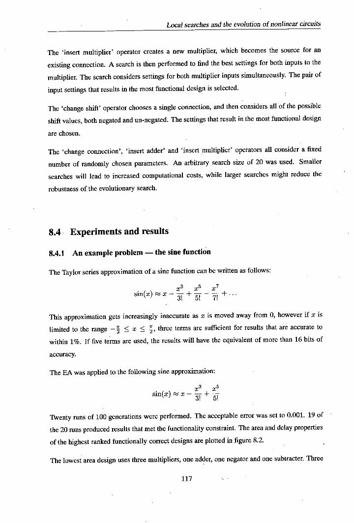
Local searches and the evolution of nonlinear circuits
The 'insert multiplier' operator creates a new multiplier, which becomes the source for an
existing connection. A search is then performed to find the best settings for both inputs to the
multiplier. The search considers settings for both multiplier inputs simultaneously. The pair of
input settings that results in the most functional design is selected.
The 'change shift' operator chooses a single connection, and then considers all of the possible
shift values, both negated and un-negated. The settings that result in the most functional design
are chosen.
The 'change connection', 'insert adder' and 'insert multiplier' operators all consider a fixed
number of randomly chosen parameters. An arbitrary search size of 20 was used. Smaller
searches will lead to increased computational costs, while larger searches might reduce the
robustness of the evolutionary search.
8.4 Experiments and results
8.4.1 An example problem - the sine function
The Taylor series approximation of a sine function can be written as follows:
x 5 x 7
This approximation gets increasingly inaccurate as x is moved away from 0, however if x is
limited to the range - x < E , three terms are sufficient for results that are accurate to
within 1%. If five terms are used, the results will have the equivalent of more than 16 bits of
accuracy.
The EA was applied to the following sine approximation:
x3 x5 sin(x) c x - + -
Twenty runs of 100 generations were performed. The acceptable error was set to 0.001. 19 of
the 20 runs produced results that met the functionality constraint. The area and delay properties
of the highest ranked functionally correct designs are plotted in figure 8.2.
The lowest area design uses three multipliers, one adder, one negator and one subtracter. Three
117

Local searches and the evolution of nonlinear circuits
I I I +
29.5
+ +
29 + +
28.5
Ca
+ ++ 'I) C
+
27.5 +
27 + +
26.5 + +
26 + +
25.5 I + 100500 101000 101500 102000 102500 103000
Area (square microns)
Figure 8.2: The properties of evolved sine circuits.
80
60
40
20
0 w
-20
-40
-60
-80 -20000 -10000 0 10000 20000
Input
Figure 8.3: The response of an evolved sine circuit, and the error when compared to an ideal sine.
10000
8000
6000
4000
2000 15 CL 0 0
-2000
-4000
-6000
-8000
-10000
response error
118

Local searches and the evolution of nonlinear circuits
roblem [Inputs I Outputs I Order [Terms [Max. error
sine 1 1 5 3 0.001
factored 1 2 1 3 7 2099.88
factored 2 2 2 3 14 915.66
random 3 x 3 3 3 2 27 1031.22
random 4 x 4 4 4 2 56 1883.06
Table 8.3: Test probhms.
multipliers are required for a fifth-order response, and at least one adder or subtracter is required
if the response is to have multiple non-zero terms. This suggests that this design has a near-
minimal area. The fastest evolved design has three multipliers and one subtracter on the critical
path, which is the minimal delay for a fifth-order response with multiple non-zero terms:
8.4.2 Application to larger problems
The EA was tested on four more problems. These problems are specified in appendix C. The
properties of these problems are listed in table 8.3. Two of these problems are factorisable; they
can be expressed in the form:
(kixi + k2x2)(k3xi + k4) (k 5x2 + k6)
where k1 . . . k6 are random real numbers between —10 and 10, and xl and x2 are the inputs.
These polynomials were used for the one output and two output cases. These test problems are
called 'factored 1' and 'factored 2'. The system was also tested on larger polynomials, which
are not factorisable. These polynomials include all of the possible first and second-order terms
for a set of inputs. Each term is multiplied by an integer between -100 and 100. These test
problems have been called 'random 3 x 3' and 'random 4 x 4', according to the numbers of
inputs and outputs.
The EA was applied to the above four problems. Twenty runs were performed for each problem.
The EA was allowed to run for 500 generations with the 'factored 1' and 'factored 2' problems,
1000 generations with the 'random 3 x 3' problem, and 2000 generations with the 'random 4 x 4'
problem. For all of the problems, the maximum acceptable error was set to one hundredth of
the sum of the squares of the coefficients.
Figure 8.4 shows the properties of the functionally acceptable non-dominated solutions from
119

Local searches and the evolution of nonlinear circuits
80
70
60
50 CO
'40 0) 0
30
20
10
n
WV V V V V
V V V
x
x x
.4 x
V
VV 0
•
X 0 0
so X XX 0 • 00 VAI V
xz P,~, ; XW XX %
• 1 *
factored 1 +
factored 2 x
random 3x3 0
I I random 4x4
0 100000 200000 300000 400000 500000 Area (square microns)
Figure 8.4: The properties of the functional solutions to the test problems.
all of the individual runs with the four problems. Some observations can be made about the
optimality of the evolved circuits. Firstly, the EA can solve the 'factored 1' problem using only
two multipliers, which is the minimum number for a cubic filter. The fastest solutions to both
the 'factored 1' and 'factored 2' problems have two multipliers on the longest path, which is
the minimum for a cubic filter. The lowest area solutions to the 'random 3 x 3' problem use
only three multipliers. The fastest solutions to the 'random 3 x 3' problem have two multipliers
on the longest path, which is not minimal for a quadratic problem, although it could, still be
Pareto optimal. The lowest area solutions to the 'random 4 x 4' problem use seven multipliers.
In comparison, in [56] the number of multipliers for a quadratic filter is defined by the rank of
the second order Volterra kernel, so an implementation of the 'random 4 x 4' problem would
require four multipliers for each output. If the terms are constructed independently and then
summed, the 'random 4 x 4' problem can be implemented using ten multipliers.
8.4.3 Scalability of the current system
The scalability of the EA system is limited by the appearance of 'junk' terms in the circuit
responses. These are terms which are not in the desired response, and which are small enough
that they do not add significant errors to the system response. Junk terms are a problem because
120

Local searches and the evolution of nonlinear circuits
they can greatly increase the computational cost of evaluating a circuit. The number of junk
terms tends to increase as the number of terms in the desired response is increased, and they
introduce a significant overhead to the evaluation of larger designs. As an example of the extent
of this problem, one of the circuits evolved for the 'random 4 x 4 problem in section 8.4.2
has a response that includes 102 junk terms as well as the 56 desired terms. In such cases,
the junk terms account for most of the computational cost of a functional evaluation. There
are two ways of avoiding this problem: either the junk terms can be discouraged, or else the
computational costs of calculating the junk terms can be reduced. The former technique places
extra constraints on the circuit designs - remember that junk terms are often functionally
insignificant. The latter technique was implemented. This was done by estimating terms that
are higher than a pre-determined order. A single term is used to represent all of the terms
of a particular order. The calculation of low-order terms is unaffected. This scheme tends to
overestimate the contribution from the high-order terms. First of all, all of the variables in the
high order terms are replaced with the dummy variable /3, according to the following rule:
- (8.3)
If there are several high order terms with the same order, the terms are merged according to the
following rule:
af3 + b3T -4 (lal + IbI)/3 (8.4)
For example, the expression:
3x + 5x + 2x 1x - 3x + (8.5)
can be expressed as the sum of low and high order terms, where here we define high-order as
being third order or higher:
(3x1 + 5x) + (2xix - 3x + x) (8.6)
The high order terms can then be approximated as follows:
(3x1 +5x)+ (2xix-3x+x) (3x1 +5x)+(2/3/3 2 —3j3+/3) (8.7)
= (3x1 +5x)+(2/33 —3/3+/3)
121

Local searches and the evolution of nonlinear circuits
Search size I Generations I Time/run (] 20 500 21.96 1 500 12.94
.1 1000 24.41 1 10000 218.91
Table 8.4: Computational costs for the 'factored 1' problem.
The third order terms can then be merged, giving the final estimate:
(3x1 +5x)+(233 —3j3+8) (3x1 +5x) +(5)33 +f35 ) (8.8)
The EA originally required about one week to perform the 20 runs with the 'random 4 x 4
problem. When the above scheme was used for the representation of terms of third or higher
order, the 20 runs could be performed in fourteen hours 2 . There was not a significant difference
between the two sets of runs in terms of design area and longest-path delay.
8.4.4 Effectiveness of the local searches
If the local searches are working correctly, the EA should produce better results in fewer gen-
erations, when compared to a non-searching EA. The computational cost of a single generation
should be higher with the local searches. The overall computational cost of the searching sys-
tem should be lower, as it should require fewer generations to produce results of a particular
quality.
The runs for the 'factored 1' problem were repeated with the search size set to 1. This ef-
fectively disabled searching for all of the evolutionary operators except for the shift-setting
operator. The shift-setting operator was left unchanged; it still searches through all possible
shift values. Runs of 500 generations were originally performed with the 'factored 1' problem,
however the non-searching EA was allowed 10,000 generations. The properties of the correct
designs are compared in figure 8.5. It can be seen that after 500 generations, the best designs
from the two systems are equivalent, while the non-searching EA shows far more variation
between the runs. When the non-searching system is allowed to run for 10,000 generations,
the results that it produces are of equivalent quality to the results from the searching system
2These times are for a Sun Blade 1500 workstation, and are only approximate. Note however that the speed increase is substantial.
122

Local searches and the evolution of nonlinear circuits
40
35
30 2
25
20 20
15 15
60000 70000 50000 90000 100000 110000 120000 60000 70000 50000 90000 100000 110000 120000
Area (square microns) Area (square morons)
40
35
30 2
25
20 1 151
60000 70000 80000 90000 100000 110000 120000
Area (square microns)
Figure 8.5: Circuit properties for the non-searching and searching EAs.
40
35
20, S500 genes
,IOOgmsemlronS
- 30 2
25 '5
123
Local searches and the evolution of nonlinear circuits
after 500 generations. This is consistent with the quality of the results being determined by the
number of evaluations, regardless of whether the evaluations are performed by the local search
or by the EA. The times taken to perform the runs 3 are listed in table 8.4. Each generation
is approximately a factor of two faster for the non-searching EA. If the results from the non-
searching EA after 10,000 generations are considered to be equivalent to the results from the
searching EA after 500 generations, then the searching EA is clearly faster.
8.5 Summary
This chapter has introduced a system for the evolutionary design of polynomial transforms.
This was achieved through the extension of the chromosome so that multipliers could be rep-
resented, and through the use of polynomials t6 represent the responses of nodes and circuit
outputs.
The local search technique that was introduced in chapter 7 was adapted for use with nonlin-
ear circuits. The shift-setting heuristic from chapter 7 could not be used, due to the fact that
nonlinear functions are not usually invertible. As in chapter 7, the local searches can save
computational effort by sharing common calculations between multiple evaluations in the local
search.
The generation of circuit responses that include all of the required terms can be problematic.
The EA has two ways of ensuring that the correct terms are present. Firstly, the initial popu-
lation is intentionally populated with 'bloated' individuals, that are likely to generate a large
number of terms. Secondly, when ranking individuals according to functionality, higher prece-
dence is given to individuals that include more of the desired terms, regardless of how well they
perform in terms of functional error.
In contrast to linear circuits, the response of a nonlinear circuit can include an arbitrarily large
amount of information. This is a major problem, as the computational costs of evaluating
a design can explode in some cases. Two solutions to this problem were considered: either
complex designs could be punished, or else the accuracy of the simulation could be reduced
when handling the more complex responses. The latter approach was implemented - the EA
was altered so that higher-order terms could be approximated by a computationally cheaper
model.
3These times are the 'user' times returned by the time command on a Sun Blade 1500 workstation.
124

Chapter 9 Enhancements
9.1 Introduction
This chapter investigates ways in which the work in earlier chapters can be extended. The
following areas are investigated:
• Pipelining and pipeline scheduling.
• Improved delay modelling.
• The use of a reduced parameter space.
• Crossover operators.
In order to investigate these areas, an EA is introduced. This basic EA is later extended in two
ways, in order to investigate the last two of the above points. For the sake of simplicity, the EA
used in this chapter does not incorporate the local searches that were introduced in chapter 7.
9.2 System overview
9.2.1 Representation
The designs are represented by a graph chromosome with a fixed number of nodes. Each node
represents an addition or a subtraction. The genes are summarised in table 9.1. The pipeline
Gene Occurrence Value
Node input source 2 per node any node or input Node input shift 2 per node integer [-4,4] Node operation 1 per node + or - Pipeline stage 1. per node integer > 0
Output source 1 per output any node or input Output shift 1 per output integer [-4,4]
Table 9.1: Summary of gene types.
125

Enhancements
stage gene, and a related repair operator, are discussed later.
The designs must be acycic. A repair operator which removes cycles is applied after every
evolutionary operation. When a cycle is detected, some of the node inputs are connected to the
design inputs, breaking the cycle.
9.2.2 Evolutionary operators
Initially, only mutation is used. Crossover operators are investigated in section 9.8.
The number of mutations is decided according to a geometric probability distribution, where the
expected number of mutations is supplied by the user. Each mutation affects a single gene. Most
mutations overwrite the gene with a randomly chosen allele. Mutations to the pipeline stage
genes randomly increment or decrement the stage number. Mutations to the 'node operation'
gene convert adders into subtracters and vice versa.
9.2.3 Populations and selection
There are three objectives: area, delay and functionality. The area and delay objectives are cal-
culated at the cell level - how this is done will be described later. The functionality objective
is calculated as follows:
MN
fuiictional error = 10 log 10 - (9.1) i=1 j=1
where H is the response matrix, and R is the desired response matrix. A logarithmic scale was
chosen to aid calculation of the niche count.
The EA is a ( + A) system, with a = A = 100. Elitism was not used. Size-2 tournament
selection was used. Tournaments are either decided by rank or by functionality alone, with a
50% probability of each option. If a tournament is a draw, the individual with the smaller niche,
count wins.
The niche count for each individual is calculated according to the sharing scheme described by
126

Enhancements
T Objective I Scale factor
Functionality 1 Area 1/470.08 Delay 1/1.728
Table 9.2: Niching parameters.
Goldberg [99]. This defines a sharing function s (d):
1—d ifd<1 s(d)
{ 0 otherwise
(9.2)
The niche count ni of individual i is defined as follows:
ni = (9.3)
where c1 3 denotes the distance between indi'iiduals i and j. The niche count is calculated in
the normalised objective space. The objectives are scaled according to the factors shown in
table 9.2. The area and delay objectives were scaled so that the niche radius is approximately
equal to the area and delay of an adder.
9.3 Pipeline scheduling
The EA produces pipelined designs. To do that, it evolves a DFG that includes scheduling
information. Pipeline registers are then inserted into the design, according to the scheduling
information. The scheduling information is encoded by a gene in each graph node. This gene
contains the number of the pipeline stage in which the node should be scheduled.
It is possible for a schedule to be invalid - for example if a component makes use of a value
that is computed in a later stage of the pipeline. In general, invalid designs can be avoided
through the use of a repair operator, by explicitly punishing invalid designs, or by ensuring that
invalid designs cannot be created. This EA uses a repair operator. Repair is more reliable than
punishment, but not as complex as ensuring that the evolutionary operators can only produce
valid schedules.
There are two ways in which an invalid schedule can be repaired. They are illustrated in fig-
127

Enhancements
Stage 0 a Stage 1
(a) invalid
schedule
ii reschedule
later E14_________ +
reschedule earlier
Figure 9.1: Two ways of repairing an invalid schedule.
ure 9.1. Nodes which are scheduled too early can be moved later (figure 9.1(b)), or alternatively
nodes Which are scheduled too late can be moved earlier (figure 9.1(c)). Using one of these
repair operators exclusively will tend to bias the search towards either ALAP or ASAP sched-
ules. For this reason one of the two repair operators is selected'at random whenever a repair
operation is needed.
9.4 Improved delay modelling
In chapter 6, the delay model was found to be very inaccurate. The inaccuracy seemed to be
the result of two different factors: the lack of a wire-load model, and the fact that delays were
calculated on a per-connection basis, rather that a per-wire basis. This chapter introduces an
improved delay model, which eliminates both of those limitations. The new model calculates
delays on a per-wire basis, incorporating wire-load delays that are independently calculated for
each wire.
The wire-load model is based upon component properties for a 0.13 4um technology library.
When calculating delays, the fanout is first calculated for each wire in the design. The fanout is
IM
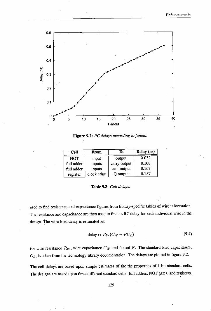
Enhancements
0.5
0.4
U) C
0.3 Co a) a
0.1
0 0
Fanout
Figure 9.2: RC delays according tofanout.
Cell From To Delay (ns)
NOT input output 0.032 full adder inputs carry output 0.108 full adder inputs sum output 0.167 register clock edge Q output 0.157
Table 9.3: Cell delays.
used to find resistance and capacitance figures from library-specific tables of wire information.
The resistance and capacitance are then used to find an RC delay for each individual wire in the
design. The wire-load delay is estimated as:
delay Rw(Cw +FCL) (9.4)
for wire resistance Rw, wire capacitance Cw and fanout F. The standard load capacitance,
CL, is taken from the technology library documentation. The delays are plotted in figure 9.2.
The cell delays are based upon simple estimates of the the properties of 1-bit standard cells.
The designs are based upon three different standard cells: full adders, NOT gates, and registers.
129

Enhancements
Subtractions are performed using the identity:
a — b=a+(-'b)-i-1 (9.5)
where '—" represents a bitwise NOT operation. Ripple adders are used. All of the standard cells
have a lx drive strength. The cell delays are summarised in table 9.3.
The new delay model is more computationally expensive than the systems used in previous
chapters. When the program was profiled, the delay modelling was found to take approximately
47% of the total execution time. This is not excessive.
9.5 Experimental methodology
Evolutionary algorithms are stochastic, and the quality of the results can vary drastically be-
tween individual runs. This makes comparisons between EAs difficult. This problem is even
more acute for multiobjective EAs, where multiple trade-offs can exist. Reliable comparisons
require multiple EA runs.
objective : _._._,_ objective A : A
a---,
I1
-
U .............
100%
75% 50%
25%
(a) objective B (b) objective B
Figure 9.3: Calculation of attainment surfaces: the four non-dominated surfaces in (a) are converted to four attainment surfaces in (b).
Attainment surfaces [110,201] are a useful tool for the evaluation and comparison of multi-
objective EAs. Attainment surfaces are found by combining the non-dominated surfaces from
multiple EA runs. An attainment surface delineates the area of the objective space that is dom-
inated by a certain proportion of the runs. For example, the 50% attainment surface marks the
edge of the region where each point is dominated by 50% of the runs. This is illustrated in
figure 9.3. Attainment surfaces are a median-like measure of performance, so they are only
130

Enhancements
reliable in areas of the objective space with a high density of non-dominated surfaces. They act
asr an estimate of the likelihood that a particular algorithm can produce solutions with the given
objective values. Attainment surfaces can be used together with statistical techniques such as
the Mann-Whitney U test, to compare the performance of multiobjective algorithms [201]. -
This chapter includes comparisons between pairs of algorithms. These comparisons can be
performed independently for each point in the objective space. The result of an individual
comparison either states that one algorithm is superior, or else states that no conclusion can be
reached.
There is a probability, p, that at least one result from a particular algorithm dominates a particu-
lar point in the objective space. If the algorithm is executed n times, the number of dominating
runs can be stated as f)n, where j5 is the observed likelihood that a run dominates the chosen
point in the objective space. Now consider two algorithms, A and B, with probabilities PA and
PB. Algorithm A could be said to be more reliable, at least with respect to the chosen point in
the objective space, if PA - PB > 0. Over many observations, the observed value 73A - PB will
tend towards PA - PB. This observed value will have a binomial distribution. The binomial
distribution involves large factorials, so a normal approximation can be used instead [2021. The
normal approximation has the following parameters:
= PAPB (9.6)
a = /J3A(1- PA) ±PB(1-PB) (9.7)
This approximation breaks down with extreme values, so it is used subject to the following
conditions: 5 TtPA :~: Th —5,
(9.8) 5 < n15B < fl —5
The null hypothesis, PA - PB < 0, therefore has the following estimated likelihood, derived
from the above normal distribution:
P(null) = (i ± erf a/)
(9.9)
If the conditions are met, PA -PB > 0, and P(null) <0.05, algorithm A is declared superior for
these particular objective values. This statistical test is repeated for other points in the objective
space, resulting in a plot that shows the areas of the objective space where each algorithm is
131

Enhancements
4
3
2 5000
7
6
5
a
3
2
0
•0
0* + + + + +
+
0_ t$*tb +
++ 0 0t XXX 0
+ ++ * is 0 x 1+hi XX 10000 15000 20 25000 30000 35000 40000 45000
Area (square microns)
depth 1 0 depth 3 0 depthS depth 2 + depth 4 X depth 6
(a) RGB to XYZ.
t)t 0
+ a
+ + *
• J * Dt+
• +40++ X 0
- 13
• +
• * t$9+ tt a
51010 10000 15000 20000 25000 300(5) 3SO00 40000 45000 50000 55000 Area (square microns)
depth 1 0 drpth 3 0 de h5 a depth 9 0 dnpth2 * depth 4 X depth 6 0
(b) 4-point DCT
$ 0
00
a
0 00
0
Figure 9.4: Solution properties according to pipeline depth.
superior, as well as the areas where no conclusion can be reached.
9.6 Initial experiments
The EA was tested on two problems: the conversion from an RGB to an XYZ colour represen-
tation, and the 4-point DCT. Fixed-point coefficients were used in both cases, and the matrices
are provided in appendix B. The acceptable functional error was set at -40 for the RGB-to-
XYZ problem, and -31.169 for the 4-point DCT problem. This latter error value was chosen
because it is equivalent to the acceptable error value used when evolving fixed-point 4-point
DCT designs in chapter 6. The RGB-to-XYZ problem was allowed 10,000 generations, while
the 4-point DCT problem was allowed 20,000 generations. One hundred runs were performed
with each problem.
Figure 9.4 shows the properties of the functionally acceptable solutions to the two test problems.
In both cases, the best solutions have pipeliuie depths of between 1 and 4 stages. The DCT
results are slightly surprising, as the entire non-dominated surface was produced by a single
run, run 23. The results produced by this run have been circled in figure 9.4(b). Run 23 was
significantly better than the other runs, but it did not evolve any unpipelined designs. This
explains why the lowest area single-stage design is dominated by a 2-stage design.
In theory, the minimum delay designs should have pipeline registers between every compu-
tational component. This would result in a delay of just less than 2ns, using this technology
132

Enhancements
140000
120000
:1 00000
000
40000
20000
0'
12
10
8
'2
S
20000 40000 80000 80000 100000 120000 140000
Design Compiler area model,
(a) Area.
2 4 6 8 10 12
Design Compiler delay model
(b) Delay.
Figure 9.5: The hardware models compared with Design Compiler.
model. In practice, such designs are unlikely to evolve using the current scheme, as every com-
ponent would be on the critical path, and nearly every change to the chromosome would lead
to an increase in critical path delay. Nevertheless, the fastest designs do approach the minimum
delay.
This EA performs worse than the EA introduced in chapter 6, both in terms of the number of
generations required, and in terms of the properties of the designs. This is evident in the results
from the 4-point DCT problem, which can be compared with the fixed-point DCT designs
evolved in chapter 6. The EA introduced in this chapter managed to create DCT designs that
require 15 additions in run 23, and 22 additions in other runs. The older system repeatedly
evolved smaller designs, including designs that use only 13 adders. This comparison is biased
towards the new EA, as the new EA was allowed 100 runs of 20,000 generations rather than
20 runs of 5000 generations. The main difference between the two systems is the evolutionary
operators. The old system uses a variety of complex operators, which were designed to be non-
destructive. The new system uses evolutionary operators which simply change a single gene.
This provides some justification for the use of the heuristic evolutionary operators in chapter 6.
The area and delay models are compared with Design Compiler's models in figure 9.5. This
comparison was performed using a selection of partially evolved 4-point DCT designs. The two
area models give identical results in all cases. The two delay models show a strong correlation.
The EA delay model consistently underestimates the delay by about one quarter. The delay
model could possibly be improved by altering some of the model parameters, although this
possibility was not investigated. The new delay model is significantly more accurate than the
133

Enhancements
Gene ]_Occurrence L_Value Node input source 2 per node any node or input Relative input shift 1 per node integer [-4,4]
Node operation 1 per node + or - Pipeline stage 1 per node integer > 0 Output source 1 per output any node or input
Table 9.4: Summary of gene types for the reduced encoding.
model used in chapter 6, which was compared with Design Compiler in figure 6.7(b).
9.7 A reduced parameter space
9.7.1 Changes to the chromosome
This section considers a more compact chromosome encoding for the EA. This encoding re-
duces the number of genes in the chromosome, while retaining the ability to represent most
useful designs.
The new chromosome encoding replaces the two genes used to represent shifts with a single
gene. This gene represents the relative shift between the two inputs. A second shift is applied
at the output of each node, however it is not encoded in the chromosome. Instead, the response
at each node output is normalised. The output of a node with un-normalised response vector a
is shifted right by s places, where s is defined as:
S=
1092 (9.10)
This ensures that the response of the node is scaled as follows:
0.5< 2 au 1 <1
The new encoding also omits the shifts at the outputs. Instead, the objective function must find
the shift that minimises the difference between the actual and desired responses at an output.
Consider an output with actual and desired response vectors a and d. The sum of squares error
134

Enhancements
between these two quantities can be expressed like this:
E=(a—dj)2 (9.12)
If the output can be shifted or negated, this becomes:
E = - d2 ) 2 (9.13)
where the scale factor k represents the shifting and negation. The ideal value of k, k', can be
derived from equation 9.13: EN = i.6 (9.14) >1i=O a2
Note that k' e R, whereas k must be expressible as a shift and an optional negation. Therefore,
k can be defined like so:
k = p2 (9.15)
for an n-bit shift, and a sign p e {-1, 1}. The values of n and p can now be fixed:
1 —1 ifk'<O, P (9.16)
1 otherwise.
n= 0.5+1092(k')j (9.17)
The above procedure assumed that the user is indifferent to the sign of the output responses.
If it is important that the outputs have the correct sign, then the sign can be fixed as p = 1.
The EA introduced in this chapter provides both options, but by default assumes that the sign
is important and p = 1. The genes in the new encoding are summarised in table 9.4.
9.7.2 Experiments
One hundred runs were performed with each system and both test problems. The results are
compared in figure 9.6, using the confidence technique described in section 9.5. The original
encoding was often found to be superior for the RGB-to-XYZ problem, while the reduced en-
coding was found to be superior in many cases with the 4-point DCT problem. The attainment
surfaces plotted in figure 9.7 also suggest that the reduced encoding is slightly better for 4-point
135

8 8
x1O
(a) RGB to XYZ.
.r.eWe) xIO
(b) 4-point DCI'.
Enhancements
Figure 9.6: Performance comparisons between the original EA (light grey) and the reduced-parameter EA (dark grey).
7
6.5
6
5.5
5 2
4.5
4
3.5
3
2.5
2 10000 15000 - 20000 25000 30000 35000
Area (square ma—)
(a) RGB to XYZ.
6.5
6
5.5
85
4.5
4
3.5
2.5 15000 50000 500005000050000 40000 45000 50000 50000
Axea (square mia)
(b) 4-point DCL
Figure 9.7: Attainment surfaces for the original and reduced-parameter EAs.
136
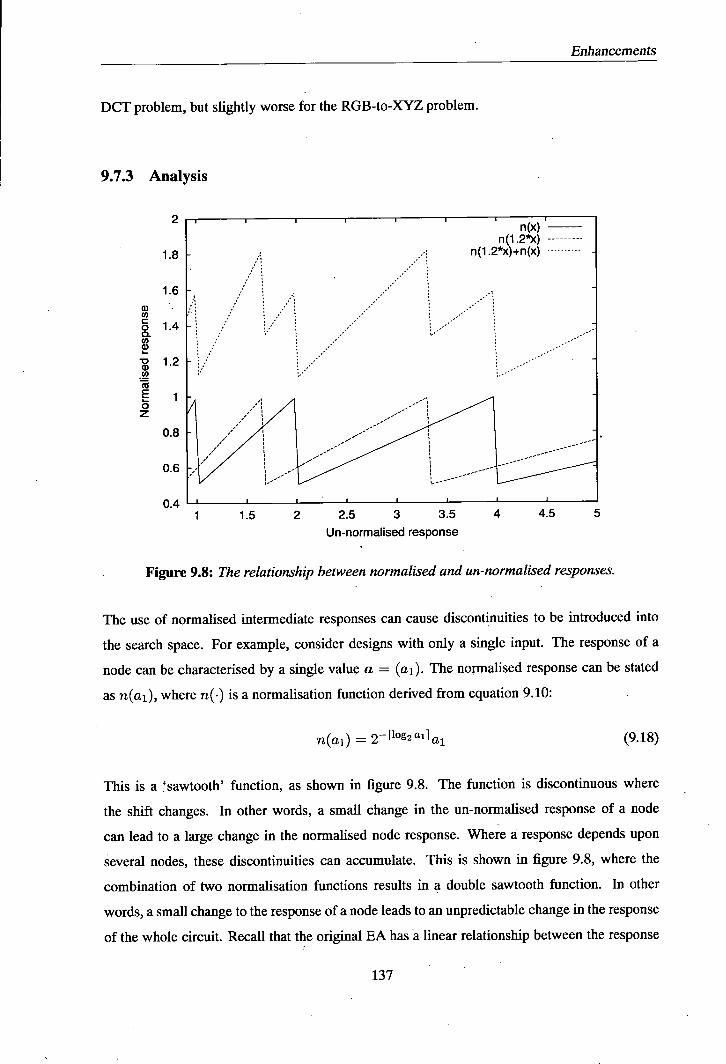
Enhancements
DCT problem, but slightly worse for the RGB-to-XYZ problem.
9.7.3 Analysis
2
1.8
1.6
a) C,) C o 1.4 0. (I) a)
1.2 C,)
as 1
0 z
0.8
0.6
0.4
n(x) n(1 .2X)
n(1.2)+n(x)
1 1.5 2 2.5 3 3.5 4 4.5 5
Un-normalised response
Figure 9.8: The relationship between normalised and un-normalised responses.
The use of normalised intermediate responses can cause discontinuities to be introduced into
the search space. For example, consider designs with only a single input. The response of a
node can be characterised by a single value a = (ai). The normalised response can be stated
as n(ai), where n(.) is a normalisation function derived from equation 9.10:
n(al) = _ I1092ail1 (9.18)
This is a 'sawtooth' function, as shown in figure 9.8. The function is discontinuous where
the shift changes. In other words, a small change in the un-normalised response of a node
can lead to a large change in the normalised node response. Where a response depends upon
several nodes, these discontinuities can accumulate. This is shown in figure 9.8, where the
combination of two normalisation functions results in a double sawtooth function. In other
words, a small change to the response of a node leads to an unpredictable change in the response
of the whole circuit. Recall that the original EA has a linear relationship between the response
137

Iij2!J
Enhancements
of a node and the response of the entire circuit. The reduced parameter system could therefore
be characterised as having a more compact encoding, but a more complex relationship between
the genotype and the functionality objective.
9.8 Neighbour crossover
9.8.1 The neighbour crossover algorithm
'0 Key
Q Parent A • Parent B \ • o Undetermined
(a) There is a neighbourhood for each parent. Node 3 could be assigned to either parent. Node 6 could be assigned to parent A.
(b) The neighbourhood for parent A is determined by the parent A edges.
(d) If node 3 is assigned to parent A, the parent A neighbourhood is expanded.
(c) The neighbourhood for parent B is determined by the parent B edges.
(e) If node 3 is assigned to parent A, the parent B neighbourhood is reduced.
Figure 9.9: One step of the neighbour crossover region growing process.
A crossover operator was introduced in chapter 4. In figure 4.13 it was shown that there is not a
138

Enhancements
clear benefit from that crossover operator. Chapters 6, 7 and 8 use a graph representation for the
chromosome, and do not use a crossover operator. This was partly due to the poor results in the
earlier BA system, but it was also partly due to the difficulty of implementing a non-destructive
graph crossover operator. In this section, a non-destructive crossover operator, the neighbour
crossover operator, is introduced.
In a graph, locality is defined by the edges. If two nodes share an edge, then those two nodes
are close to each other. Nodes with a higher degree of separation are further apart, while
nodes that share multiple edges are closer together. The neighbour crossover algorithm is based
upon the principle that if two nodes are local to each other, it should be unlikely that they are
separated. Conversely, if two nodes are only distantly connected, they should be more likely to
be separated by crossover.
The nodes in the chromosome have an index, and this is used to define which nodes correspond
in the two parents. A node with index i in the child will therefore be a copy of the node with
index i in one of the parents. Note that the index defines a correspondence between nodes in
different chromosomes, but it is not used to define a linear ordering for the nodes in a single
chromosome. The purpose of the crossover operator is to determine which nodes come from
which parent.
A node in the child can be marked as being derived from one or other parent, or else it can
be marked as 'undetermined'. When the algorithm starts, all nodes are marked as undeter-
mined, and the algorithm finishes when all nodes have been assigned a parent. Two nodes are
neighbours if there is an edge between them.
The neighbour crossover algorithm is as follows:
• Mark all nodes as undetermined.
• Define two neighbour lists, which are initially empty. One neighbour list corresponds to
each parent.
• While there are undetermined nodes:
- Choose a parent P.
- If the neighbour list Np is empty, insert a randomly chosen undetermined node into
Np.
139
Enhancements
- Pick a random node n E Np, assign it to parent P, and remove it from both neigh-
bour lists.
- Insert all of the undetermined neighbours of n into Np; if there are multiple edges
between n and an undetermined node n', insert n' multiple times. This step uses
the edges from parent P to determine the neighbours.
• Copy node information from the parents according to the how the nodes are labelled.
• Copy edges from the parents according to how the destination nodes are labelled.
Neighbours are determined using the edges from one or other parent. In other words, the
neighbours for a node n, assigned to parent P, are determined according to the, edges from
parent P. Figure 9.9 illustrates one step of this algorithm.
9.8.2 Experiments
The neighbour crossover algorithm was compared with the following alternative schemes:
• no crossover,
• 2-point crossover,
• uniform crossover.
All of the crossover operators operate at the node level; they always copy all of the genes in
a node from the same parent. The crossover rate was set to 100%. A mutation rate of 1 was
used when crossover was available, while a mutation rate of 2 was used when crossover was
disabled.
In figure 9.10, neighbour crossover is compared with the other schemes, using both test prob-
lems. Neighbour crossover is superior over large parts of the objective space in all but one case.
In figure 9.10(a), it was found that disabling crossover often gives better results for the RGB-to-
XYZ problem, although neighbour crossover is superior for some of the most important points
closer to the origin.
In figure 9.11, the 5% and 10% attainment surfaces are shown for the two problems. The
neighbour crossover attainment surfaces dominate the other surfaces in all cases, with the most
pronounced differences evident with the 4-point DCT problem.
140

Enhancements
I
—41-11 aio
(b) No crossover, 4-point DC-
(a) No crossover, RGB to XYZ. r--W"
I
I I
(c) Uniform crossover, RGB to XYZ.
aio•
(d) Uniform crossover, 4-point DCI'.
a; , 1
o.s i is 2 as a
(e) 2-point crossover, RGB to XYZ.
iO
(I) 2-point crossover, 4-point DC'!'.
Figure 9.10: Neighbour crossover (light grey) compared to other techniques (dark grey).
141

Enhancements
5.5
5
4.5
0 3.5
3
2.5
2
7
6.5
6
5.5
5
4.5
4
3.5
3
2.5
no crossover neighbour crossover
2-point crossover .......... uniform crossover
6
5.5
5
4.5
3.5
3
7-s
5000 10000 15000 20000 25000 30000 35000 40000 45000 50000
Area (square micro(rs(
(a) RGB tp XYZ, 5%.
iw crossover neighbour crossover --
2-point crossover .......... uniform crossover
10000 15000 20000 25000 30000 35000 40000
Area (square mfooins)
(c) 4-point DCT, 5%.
5000 10000 15000 20000 25000 30000
Area (square microns(
(b) RGB to XYZ, 10%.
6 rio Crossover
neighbour crossover 1 2-point CrOssove............
unrfonn crossover
4.5
3.5
2.5 10000 15000 20000 25000 30000 35000 40000 45000
Area (square mlcrons(
(d) 4-point DCT, 10%.
Figure 9.11: 5% and 10% attainment surfaces, with various crossover operators.
142
Enhancements
9.9 Summary
This chapter has investigated several improvements over the EAs introduced in earlier chapters.
These improvements include:
• pipelining,
• improved delay modelling,
• a more compact chromosome encoding,
a non-destructive crossover operator.
The EA introduced in this chapter did not make use of local searches, and the evolutionary
operators were designed for simplicity rather than constructiveness. This meant that the EA
was not as effective as the EAs in previous chapters. In particular, it was shown to be worse
than the EA introduced in chapter 6. This provides some justification for the design decisions
in earlier chapters.
The introduction of pipelining caused a clear conflict between the area and longest-path delay
objectives. The EA is capable of evolving designs with relatively few pipeline stages. It did
not evolve maximally pipelined designs. Scheduling becomes more complex as the number of
stages is increased, so it is likely that the lack of highly pipelined designs is due to limitations of
the current scheduling technique. The delay for the pipelined designs was close to the minimum
possible delay, the delay of an adder and a register, so extra pipelining would only have a minor
effect.
In chapter 6, two major deficiencies were identified in the delay model. These were the omis-
sion of wire-load modelling, and the fact that delays were modelled on per-connection basis,
rather than a per-wire basis. This chapter introduces a new wire model, that addresses both of
these deficiencies. The new wire model was found to more closely agree with the Design Com-
piler delay model. The new model is not perfect; it tends to underestimate delays by more than
25%. It is possible that these inaccuracies could be reduced through the use of more accurate
parameter settings. While the new delay model is more computationally expensive, it is not
excessively so.
A reduced parameter chromosome encoding was investigated. This reduces the number of
genes required to represent shifts in the chromosome by making use of the automatic normali-
143

Enhancements
sation of shifts. This resulted in a reduced variable space, without significantly impacting upon
the representation of useful designs. The net effect is to increase the probability that a particular
chromosome is useful. This reduction in the size of the chromosome possibly comes at the cost
of an increase in the number of discontinuities in the objective landscape. When tested, the re-
duced encoding was found to be inferior to the original scheme for the RGB-to-XYZ problem,
but superior for the more difficult 4-point DCT problem.
The neighbour crossover operator was introduced. This is a non-destructive graph crossover
operator. It is designed so that the parent chromosomes are spliced together at relatively few
points. This is achieved by taking account of the degree of separation between nodes when
performing crossover. The neighbour crossover operator ensures that nodes with a high degree
of connectedness are likely to be taken from the same parent. It was shown that the neighbour
crossover operator increases the probability that good quality results are evolved, in comparison
with other crossover operators or no crossover.
144

Chapter 10
Conclusions
10.1 Introduction
This chapter concludes this thesis. In section 10.2, the contents of individual chapters are
reviewed. Section 10.3 lists some specific conclusions that can be drawn from the results in
this thesis. In section 10.4, some possible directions for future work are listed. Finally, in
section 10.5 the contents of the thesis are summarised, with reference to the thesis statement.
10.2 Review of thesis contents
Chapters 2 and 3 provided a review of the existing literature which is relevant to this thesis;
In chapter 4, an BA for the evolution of multiplierless FIR filters was introduced. This EA
takes a frequency domain specification as input, and produces a set of structural filter designs
as output. The BA has three objectives: functionality, low silicon area, and low longest-path
latency. The area and delay objectives are based on figures taken from a real technology library.
The EA used several 'heuristic' evolutionary operators. These evolutionary operators treat the
chromosome as a graph, and perform operations which are likely to lead to improvements to
the design. The BA was tested on several different problems. Crossover was found to be of
no benefit to the EA. The evolved filters were found to be competitive with filters produced by
other filter design systems.
In chapter 5, the evolution of multistate sequential hardware was investigated. The BA intro-
duced in chapter 4 was extended so that it could generate filters with multiplication blocks that
operate over two cycles. These filters are slower but have lower area requirements. The EA was
able to perform scheduling, allocation and binding in parallel with circuit design, so hardware
costs could influence the schedule. While modest area savings were achieved, the savings were
limited by two factors. Firstly, the multiplication block is only part of the filter area, and the
accumulation block generally consumes most of the area. Secondly, the area cost of an adder is
/
145

Conclusions
not much higher than the areas of registers and multiplexors, so the overheads incurred by mul-
tistate operation cancel out a significant part of the savings. Multiplication blocks that operate
over more than two states were also considered. When operating over more than two states,
finding the most efficient topology for the registers and multiplexors becomes a hard problem.
The techniques introduced in this chapter could be applied to other problems, and in particular
with components that have a high area cost.
Chapters 6, 7 and 8 all dealt with similar EAs. Chapter 6 introduced an EA for the evolution
of multiplierless linear transforms. The transforms are specified by a coefficient matrix, and
the resulting circuit designs are constructed from adders, subtracters, negators and shifts. As
before, the designs were evolved with the objectives of functionality, low area and low longest-
path latency. The EA made use of a graph chromosome, which was altered by a set of heuristic
mutation operators. Crossover was not used. It was found that the EA could compete with the
Iterative Matching algorithm [36] in terms of component counts. The fastest evolved designs
were found to be slower than CSD transform implementations, although the evolved designs
are still more area-efficient than the CSD results. It was found that the EA is more successful
if it is allowed to use right-shifts in the evolved designs.
The EA in chapter 6 could generate three different types of hardware: bit-serial, fixed-width
bit-parallel, and variable-width bit-parallel. The accuracy of the area and delay models was
investigated - the area model was found to be acceptable, however the delay model was found
to be inaccurate. The delay model inaccuracies were probably caused by two factors: the lack
of a wire-load model, and the fact that delays were modelled at a component level rather than
at the level of individual wires.
In chapter 7, the EA from chapter 6 was extended through the introduction of local searches.
The local searches are based on a linear decomposition of the design, and implemented within
the evolutionary operators. The local searches are capable of rapidly evaluating the function-
ality of large numbers of mutated designs. This is achieved through the reuse of intermediate
values during the local search. A second improvement in search efficiency is achieved through
the automatic calculation of near-optimal shift settings during the search. It was shown that
the local searches greatly increase the efficiency of the EA. This means that that the EA can be
applied to problems for which evolutionary design would otherwise be infeasible.
In chapter 8, an EA for the design of polynomial transform circuits is introduced. This EA is
146

Conclusions
similar to the EM introduced in chapters 6 and 7, however it can produce designs that contain
multipliers and have a nonlinear response to the input signals. The designs are specified by
a set of polynomials, where each. polynomial describes an output response in terms of the
inputs. This EA uses a variation of the local searches that were introduced in chapter 7. The
local searches used in chapter 8 were not as powerful as the searches used in chapter 7, as
there is no way to efficiently calculate good shift settings in a nonlinear design. It was found
that the EA would often fail to generate many of the terms that. are in the specified response.
Two solutions were devised. Firstly, the initial population was created in a way that is likely to
result in responses with many terms. Secondly, functionality was scored in a way that explicitly
rewarded designs that include more of the desired response terms. Extra terms were also found
to be a problem, as they could drastically slow down the evaluation of functionality. This
problem could be solved with a penalty function, or by using estimated responses rather than
exact responses. The latter of these options was implemented, and was found to be effective.
Chapter 9 introduced an EA which can produce designs for pipelined linear transforms. It
combines pipeline scheduling with the evolution of functionality, so that both of these tasks
can take account of the objectives. The EA was capable of producing combinatorial designs
and designs with relatively few pipeline stages. It was not capable of producing maximally
pipelined designs. Nevertheless, the fastest evolved designs were close to the minimum delay.
Chapter 9 introduced a new delay model, without deficiencies that were identified in chapter 6.
The new delay, model was found to be better than the earlier models, although it could possibly
benefit from more accurate parameter settings. Chapter 9 investigated two ways in which the
performance of the EA could be improved: through the use of a more compact chromosome
encoding scheme, and with a novel crossover operator. The new encoding scheme was based on
The use of normalised shifts. It resulted in an objective landscape which was smaller but more
complex, and produced improved results some of the time. The, neighbour crossover operator
is a graph crossover operator which was designed to be largely non-destructive. In most tests
the neighbour crossover was found to be superior to other crossover operators, or no crossover
operator. The neighbour crossover operator could be applied to other problems.
103 Specific findings
This section presents a variety of conclusions, which stem from the research in this thesis.
147
Conclusions
While most research into evolutionary hardware design has focussed on gate-level circuits, EAs
can also be used for the creation of designs based upon high-level arithmetic components. This
thesis demonstrated the application of EAs to several high-level synthesis problems.
Graph chromosomes were found to be a useful and very intuitive representation for digital
circuits. The use of a graph chromosome representation greatly simplifies the mapping between
the genotype and the phenotype. The main drawback for graph chromosomes is that they
require many complicated evolutionary operators in order to properly search the design space.
Most evolutionary operators were found to be destructive in a majority of cases. In other words,
most changes to a semi-functional circuit are detrimental to functionality. Both crossover and
mutation operators were found to be destructive. This observation led to the development of
evolutionary operators that are designed to be less damaging to the chromosome; namely the
heuristic mutation operators and the neighbour crossover operator.
There are many improvements to a circuit design, which although obvious to a human de-
signer, are unlikely to be discovered by an evolutionary algorithm. For example, some of the
circuits examined in chapter 4 could be trivially improved by strength reduction and common
subexpression elimination operations. An evolutionary algorithm can not discover these im-
provements because they involve the simultaneous modification of several genes. This problem
can be overcome through the development of a rich set of evolutionary operators, which can
explicitly perform such improvements.
The local searches which were described in chapters 7 and 8 produced major increases in the
performance of the EA. The use of local searches combined with an EA results in a hybrid
algorithm which combines the power and robustness of an BA with the speed of hiliclimbing.
Evolutionary algorithms can perform scheduling in parallel with other circuit design tasks. This
approach is in contrast to conventional methods, which typically treat scheduling as one step
in the design process. By iteratively performing scheduling in parallel with other design tasks,
the BA ensures that all aspects of the design can be directly influenced by the objectives.
It is very useful if the response of a design can be completely characterised. This not only
aids evaluation of the functionality objective, but also ensures that the user can be sure of
the response of the design to all possible inputs. The response of linear digital circuits is
compact and easy to calculate. For most classes of nonlinear digital circuits, the complexity of
148

Conclusions
the response is likely to grow as the number of components is increased. This can make the
calculation of exact responses impractical for nonlinear circuits, as was found in chapter 8. If
this happens, approximate responses can be used instead.
There is often a large amount of variation in solution quality between different EA runs. This
variation can be reduced by combining the results from multiple runs. Evolutionary algorithms
do not guarantee a worst-case performance. If such a guarantee is required, a non-stochastic
method could be used either to seed the EA population, or else to provide back-up solutions in
the case that the EA fails to produce useful results.
Synthesis problems often have more than one objective. Multiobjective evolutionary algorithms
are a powerful technique for the discovery of multiple non-dominated solutions to multiobjec-
tive problems.
Accurate hardware modelling is useful, because it lets the EA correctly weigh up the costs
of different designs. This thesis has demonstrated the use of accurate models of the area and
longest-path delay of a design. While accuracy leads to some extra computational costs, the
models used in this thesis were still fast enough to be used as objectives, even when hundreds
of thousands of evaluations were required.
10.4 Directions for further research
• This thesis has considered the EA in isolation from conventional design tools, however
it is likely that a single project could make use of both conventional and evolutionary
synthesis techniques. The combination and integration of these two distinct synthesis
techniques could be investigated.
• A power objective would be very useful. This would involve the development of a fast
approximate power model. The power objective is likely to correlate with the area objec-
tive, so the area objective could possibly be removed.
• The decomposition of large designs could be investigated. Large design specifications
could be divided into module specifications, which could then be synthesised by an EA.
• Hierarchy is commonly used to simplify design tasks, and there have been some investi-
gations into the automatic determination of modular structures [106]. Could hierarchical
149
Conclusions
digital designs be evolved for high-level digital design problems, and is there any benefit
over non-hierarchical techniques?
• If multiplexors were to be introduced as a component, the evolved designs could have a
degree of programmability. This could either be used for the implementation of multiple
functions (for example, filters which can switch between two different responses), or else
to increase robustness to component failures.
10.5 Summary
The thesis statement introduced in chapter 1 is as follows:
To investigate ways in which multiobjective evolutionary algorithms can be used for high-level digital circuit design, and to find ways in which the effi-ciency and usefulness of these EAs can be improved.
This can be divided into three main areas:
To demonstrate the use of EAs for the synthesis of several important classes of hardware.
To demonstrate multiobjective evolution, where the objectives are based upon accurate
hardware models.
To increase the performance and capabilities of evolutionary algorithms for these prob-
lems, and in general.
These aims have been approached as follows.
Regarding the first aim, EAs have been developed for the creation of FIR filters, linear transform
circuits and polynomial transform circuits. The evolution of multistate sequential designs and
the evolution of pipelined designs were also investigated. These classes of design are used in a
wide variety of real-world applications.
Regarding the second aim, the EAs all used the objectives of functionality, low area, and low
longest-path delay. The area and delay objectives were calculated using accurate hardware
models, using figures derived from real technology libraries. Crucially, the computational costs
150

Conclusions
of hardware modelling are low enough that this approach is viable. The use of accurate hard-
ware models directed the search towards the most efficient hardware designs. Where there is a
conflict between the objectives[the use of a multiobjective EA enables the discovery of multiple
trade-off solutions, from which the user can select the most appropriate design for a particular
situation.
Regarding the final aim, several different techniques were developed. These include the use of
graph encodings together with heuristic operators, the local searches introduced in chapters 7
and 8, the reduced parameter-space encoding from chapter 9, and the neighbour crossover
operator. These techniques led to substantial increases in the, performance and capabilities
of the EM. These techniques could potentially be adapted for application to other evolutionary
design problems.
Evolutionary algorithms were found to be a powerful method for the discovery of efficient
circuit designs. Their major strengths are robustness in the face of highly complex circuit design
problems, and the ability to work with accurate hardware models and multiple objectives. This
thesis has investigated how evolutionary algorithms can be applied to the creation of useful
digital circuit designs, and how the performance of evolutionary algorithms can be improved.
Hopefully, this research will lead to the development and use of commercial digital circuit
synthesis tools which incorporate evolutionary methods.
151

Appendix A Publications
A.! Refereed publications
Robert Thomson and Tughrul Arslan, "An Evolutionary Algorithm for the Multi-objective Op-timisation of VLSI Primitive Operator Filters", in Proceedings of the 2002 Congress on Evolu-
tionary Computation, pages 37-42, May 2002.
Robert Thomson and Tughrul Arsian, "Evolvable Hardware for the Generation of Sequential Filter Circuits", in Proceedings of the 2002 NASA/DoD Conference on Evolvable Hardware,
pages 17-25, July 2002.
Robert Thomson and Tughrul Arslan, "The Evolutionary Design and Synthesis of Non-Linear
Digital VLSI Systems", in Proceedings of the 2003 NASA/DoD Conference on Evolvable Hard -
ware, pages 125-134, July 2003.
Robert Thomson and Tughrul Arslan, "On the Impact of Modelling, Robustness, and Diver-sity to the Performance of a Multi-Objective Evolutionary Algorithm for Digital VLSI System
Design", in Proceedings of the 2003 Congress on Evolutionary Computation, pages 382-389,
volume 1, December 2003.
B. Hounsell , T. Arslan and R. Thomson, "Evolutionary design and adaptation of high perfor -
mance digital filters within an embedded reconfigurable fault tolerant hardware platform", in Soft Computing - A Fusion of Foundations, Methodologies and Applications, Volume 8, Num-
ber 5, pages 307-317, April 2004.
E. Stefatos, W. Han, T. Arslan, and R. Thomson, "Low-Power Reconfigurable VLSI Archi-tecture for the Implementation of FIR Filters", in Proceedings of the 19th IEEE International
Parallel and Distributed Processing Symposium, April 2005.
Robert Thomson and Tughrul Arslan, "Techniques for the Evolution of Pipelined Linear Trans-
forms", in Proceedings of the 2005 Congress on Evolutionary Computation, Volume 3, pages
2476-2483, September 2005.
A.2 Patent application
The University of Edinburgh, Tughrul Arslan, Robert Graham, and Robert Thomson, "System and Method for Rapid Prototyping of ASIC Systems", international patent application number
W02004068535, August 2004.
153
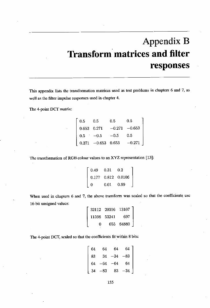
Appendix B Transform matrices and filter
responses
This appendix lists the transformation matrices used as test problems in chapters 6 and 7, as
well as the filter impulse responses used in chapter 4.
The 4-point DCT matrix:
0.5 0.5 0.5 0.5
0.653 0.271 —0.271 —0.653
0.5 —0.5 —0.5 0.5
0.271 —0.653 0.653 —0.271
The transformation of RGB colour values to an XYZ representation [13]:
0.49 0.31 0.2
0.177 0.812 0.0106
0 0.01 0.99
When used in chapters 6 and 7, the above transform was scaled so that the coefficients use
16-bit unsigned values:
32112 20316 13107
11598 53241 697
0 655 64880
The 4-point DCT, scaled so that the coefficients fitwithin 8 bits:
64 64 64 64
83 34 —34 —83
64 —64 —64 64
34 —83 83 —34
155

Transform matrices and filter responses
The 8-point DCT, scaled so that the coefficients fit within 8 bits:
64 64 64 64 64 64 64 64
88 75 50 18 —18 —50 —75 —88
83 34 —34 —83 —83 —34 34 83
75 —18 —88 —50 50 88 18 —75
64 —64 —64 64 64 —64 —64 64
50 —88 18 75 —75 —18 88 —50
34 —83 83 —34 —34. 83 —83 34
18 —50 75 —88 88 —75 50 —18
The 8-point DHT, scaled so that the coefficients fit within 8 bits:
64 64 64 64 64 64 64 64
64 91 64 0 —64 —91 —64 —0
64 64 —64 —64 64 64 —64 —64
64 0 —64 91 —64 —0 64 —91
64 —64 64 —64 64 —64 64 —64
64 —91 •64 —0 —64 91 —64 0
64 —64 —64 64 64 —64 —64 64
64 —0 —64 —91 —64 0 64 91
The following filter coefficient sets were derived using SPW. They were used for some of
the comparisons in chapter 4. These coefficient sets are all symmetrical around the central
coefficient, so the duplicated coefficients are omitted here.
Filter Coefficients
30dB low pass (-1,14,44,77,92 ....
40dB low pass (-9,1,62,183,313,369 ....
50dB low pass (-29, —67, —18,243,721, 1214, 1426,...)
30dB high pass (-3,16, —11, —39,75,...)
40dB high pass (-15,10,58, —52,-146,288....
50dB high pass (39, —154,130,163, —134, —630,1167 ....
156
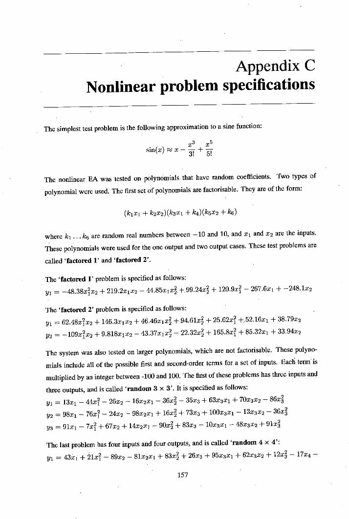
Appendix C Nonlinear problem specifications
The simplest test problem is the following approximation to a sine function:
x 3 x 5 sin(x) a: - --+
The nonlinear EA was tested on polynomials that have random coefficients. Two types of
polynomial were used. The first set of polynomials are factorisable. They are of the form:
(kixi + k2x2)(k3xi + k4) (k5xa + k6)
where k1 . . . k6 are random real numbers between —10 and 10, and x1 and a:2 are the inputs.
These polynomials were used for the one output and two output cases. These test problems are
called 'factored 1' and 'factored 2'.
The 'factored 1' problem is specified as follows:
yi = 48.38XX2 + 219.2X1X2 - 44.85xi4.+ 99.24x + 120.9x - 267.6xi + —248.1x2
The 'factored 2' problem is specified as follows:
= 62.48xx2 + 146.3x1x2 + 46.46xix + 94.61x + 25.62x +52.16xi + 38.79x2
112 = -109xx2 + 9.818x1x2 - 43.37x1x - 22.32x + 165.8x + 85.32xi + 33.94X2
The system was also tested on larger polynomials, which are not factorisable. These polyno-
mials include all of the possible first and second-order terms for a set of inputs. Each term' is
multiplied by an integer between -100 and 100. The first of these problems has three inputs and
three outputs, and is called 'random 3 x 3'. It is specified as follows:
yj = 13x1 - 44x 2 - 26x2 - 16x2x - 36x - 35x3 + 63x3x + 70x3x2 - 86x
112 = 98x1 - 76x - 24x2 - 98x2xi + 16x + 73x3 + 100x3x1 - 13x3x2 - 36x
= 9lxi - 7x + 67x2 + 14x2x1 - 90x + 83x3 - lOx3xi - 48x3x2 + 9laj
The last problem has four inputs and four outputs, and is called 'random 4 x 4':
yi = 43xi + 21x - 89x2 - 81x2x + 83x + 26x3 + 95x3x1 + 62x3x2 + 12x - 17x4 -
157

Nonlinear problem specifications
82x4x1 + 58x4x2 + 87x4x3 - 74x
Y2 = —82x1 - 61x + 35x2 + 8x2x1 - 71x + 90x3 - 43x3x1 - 25x3x2 - 2x - 91x4 +
24x4x1 - 92x4x2 - 22x4x3 - 39r4
= 79x1 + 2Ox 2 + 15x2 + 41x2x1 - 16x+ 85x3 + 87x3x1 + 43x3x2 - 39x - 74x4 -
69x4x1 - 45x4x2 + 9x4x3 - 4x
= 15x - 69x 2 + 52x2 + 20x2x1 - 14x + 7lx3 - 99x 3 x 1 - 78x3x2 - 35x + 49x4 +
29x4x1 - 60x4x2 + 65x4x3 - 5x
158
References
T. M. Panicker and V. J. Mathews, "Parallel-cascade realizations and approximations of truncated Volterra systems," in IEEE International Conference on Acoustics, Speech, and Signal Processing, vol. 3, pp. 1589-1592, May 1996.
T. M. Panicker and. V. J. Mathews, "Parallel-cascade realizations and approximations of truncated Volterra systems," IEEE Transactions on Signal Processing, vol. 46, pp. 2829-
2832, Oct. 1998.
D. Suckley, "Genetic algorithm in the design of FIR filters," lEE Proceedings Circuits,
Devices and Systems, vol. 138, pp. 234-238, Apr. 1991.
D. W. Redmili, D. R. Bull, and E. Dagless, "Genetic synthesis of reduced complexity filters and filter banks using primitive operator directed graphs," in lEE Proceedings -
Circuits, Devices and Systems, pp. 303-310, Oct. 2000.
M. R. Garey and D. S. Johnson, Computers and Intractability /A Guide to the Theory of
NP-Completeness. W. H. Freeman and Company, 1979.
T. Kalganova and J. Miller, "Evolving more efficient digital circuits by allowing circuit layout evolution and multi-objective fitness," in Proceedings of the First NASA/DoD
Workshop on Evolvable Hardware (A. Stoica, D. Keymeulen, and J. Lohn, eds.), pp. 54-
63, July 1999.
B. I. Hounsell and T. Arslan, "A novel genetic algorithm for the automated design of performance driven digital circuits," in Proceedings of the Congress on Evolutionary
Computation, vol. 1, pp. 601-608, July 2000.
A. Hernandez-Aguirre, C. A. Coello, and B. P. Buckles, "A genetic programming ap-proach to logic function synthesis by means of multiplexers," in Proceedings of the First
NASA/DoD Workshop on Evolvable Hardware (A. Stoica, D. Keymeulen, and J. Lohn,
eds.), pp. 46-53, July 1999.
S. K. Mitra and J. F. Kaiser, Handbook for digital signal processing. John Wiley & Sons,
Inc., 1993.
J. G. Proakis and D. G. Manolakis, Digital signal processing: principles, algorithms, and
applications. 866 Third Avenue, New York, New York 10022: Macmillan Publishing
Company, 2 ed., 1992.
R. E. Crochiere and A. V. Oppenheim, "Analysis of linear digital networks," Proceedings
of the IEEE, vol. 63, pp. 581-595, Apr. 1975.
T. W. Parks and J. H. McClellan, "Chebyshev approximation for nonrecursive digital filters with linear phase," IEEE Transactions on Circuits and Systems, vol. 19, pp. 189-
194, Mar. 1972.
159

References
R. W. G. Hunt, The Reproduction of Colour, ch. 8, p. 143. Fountain Press, fifth ed., 1995.
W. B. Pennebaker and J. L. Mitchell, JPEG still image data compression standard. Van Nostrand Reinhold, 1992.
R. J. Clarke, Digital compression of still images and video. Academic Press, 1995.
C. S. Bumis, R. A. Gopinath, and H. Guo, Introduction to wavelets and wavelet trans-forms: a primer. Prentice-Hall, Inc., 1998.
W. Sweldens, "The lifting scheme: A custom-design construction of biorthogonal wavelets," Applied and Computational Harmonic Analysis, vol. 3, PP. 186-200, Apr. 1996.
ISO!ITU-T, ISO/fEC 15444-1:2004 Information technology —JPEG 2000 image coding system: Core coding system, Sept. 2004.
M. Schetzen, The Volterra and Wiener Theories of Nonlinear Systems. Krieger Publish-ing Company, 1980.
G. W. Reitwiesner, "Binary arithmetic," Advances in Computers, vol. 1, pp. 231-308, 1960.
A. Avizienis, "Signed-digit number representations for fast parallel arithmetic," IRE Transactions on electronic computers, vol. 10, pp. 389-400, 1961.
H. L. Garner, "Number systems and arithmetic," Advances in Computers, vol. 6, pp. 131-194, 1965.
K. Hwang, Computer Arithmetic: Principles, Architecture, and Design. John Wiley and Sons, Jan. 1979.
Y. C. Lim and S. R. Parker, "FIR filter design over a discrete powers-of-two coeffi-cient space," IEEE Transactions on Acoustics, Speech, and Signal Processing, vol. 31, Pp. 583-591, June 1983.
H. Samueli, "An improved search algorithm for the design of multiplierless FIR filters with powers-of-two coefficients," IEEE Transactions on Circuits and Systems, vol. 36, pp. 1044-1047, July 1989.
R. Bernstein, "Multiplication by integer constants," Software : practice and experience, vol. 16, no. 7, pp. 641--652, 1986.
A. G. Dempster and M. D. Macleod, "Constant integer multiplication using minimum adders," fEE Proceedings -Circuits, Devices and Systems, vol. 141, pp. 407-413, Oct. 1994.
A. G. Dempster and M. D. Macleod, "Multiplication by an integer using minimum adders," in lEE Colloquium on Mathematical Aspects of Digital Signal Processing, pp. 11/1-11/4, Feb: 1994.
- 160

References
A. Dempster, Digital filter design for low-complexity implementation. PhD thesis, Cam-bridge University, Signal processing and communications laboratory, Department of en-
gineering, May 1995.
0. Gustafsson, A. G. Dempster, and L. Wanhammar, "Extended results for minimum-adder constant integer multipliers," in IEEE International Symposium on Circuits and
Systems, pp. 1-73-1-76, 2002.
D. Li, "Minimum number of adders for implementing a multiplier and its application to the design of multiplierless digital filters," IEEE Transactions on Circuits and Systems
II: Analog and Digital Signal Processing, vol. 42, no. 7, pp. 453-460, 1995.
A. G. Dempster and M. D. Macleod, "Comments on "minimum number of adders for im-plementing a multiplier and its application to the design of multiplierless digital filters"," IEEE Transactions on Circuits and Systems II: Analog and Digital Signal Processing,
vol. 45, no. 2, pp. 242-243, 1998.
D. R. Bull and D. H. Horrocks, "Primitive operator digital filters," lEE Proceedings -
Circuits, Devices and Systems, vol. 138, pp. 401-412, June 1991.
A. G. Dempster and M. D. Macleod, "Use of minimum-adder multiplier blocks in FIR digital filters," IEEE Transactions on Circuits and Systems II: Analog and Digital Signal Processing, vol. 42, pp. 569-577, Sept. 1995.
A. G. Dempster and M. D. Macleod, "General algorithms for reduced-adder integer mul-tiplier design," Electronics Letters, vol. 31, pp. 1800-1802, Oct. 1995.
M. Potkonjak, M. B. Srivastava, and A. P. Chandrakasan, "Multiple' constant multipli-cations: efficient and versatile framework and algorithms for exploring common subex-pression elimination," IEEE Transactions on Computer-Aided Design of Integrated Cir-cuits and Systems, vol. 15, pp. 151-165, Feb. 1996.
M. Mehendale, S. D. Sherlekar, and G. Venkatesh, "Synthesis of multiplier-less FIR filters with minimum number of additions," in Digest of Technical Papers, IEEE IA CM International Conference on Computer-Aided Design, pp. 668-671, Nov. 1995.
A. Matsuura, M. Yukishita, and A. Nagoya, "An efficient hierarchical clustering method for the multiple constant multiplication problem," in Proceedings of the Asia and South
Pacific Design Automation Conference, pp. 83-88, Jan. 1997.
R. Pako, P. Schaumont, V. Derudder, S. Vernalde, and D. Iiuraëková, "A new algorithm for elimination of common subexpressions," IEEE Transactions on Computer-Aided De-
sign of Integrated Circuits and Systems, vol. 18, pp. 58-68, Jan. 1999.
R. I. Hartley, "Subexpression sharing in filters using canonic signed digit multipliers," IEEE Transactions on Circuits and Systems II: Analog and Digital Signal Processing, vol. 43, pp. 677-688, Oct. 1996.
R. I. Hartley, "Optimization of canonic signed digit multipliers for filter design," in IEEE
International Sympoisum on Circuits and Systems, pp. 1992-1995, June 1991.
161

References
M. Martinez-Peiró, E. I. Boemo, and L. Wanhammar, "Design of high-speed multi-plierless filters using a nonrecursive signed common subexpression algorithm," IEEE Transactions on Circuits and Systems II: Analog and Digital Signal Processing, vol. 49, pp. 196-203, Mar. 2002.
1.-C. Park and H.-J. Kang, "Digital filter synthesis based on an algorithm to generate all minimal signed digit representations," IEEE Transactions on Computer-Aided Design of Integrated Circuits and Systems, vol. 21, pp. 1525-1529, Dec. 2002.
1.-c. Park and H.-J. Kang, "Digital filter synthesis based on minimal signed digit rep-resentation," in Proceedings of the Design Automation Conference, pp. 468-473, June 2001.
A. G. Dempster, 0. Gustafsson, and J. 0. Coleman, "Towards an algorithm for matrix multiplier blocks," in Proceedings of the European Conference on Circuit Theory and Design, pp. 1119-12, Sept. 2003.
A. Chatterjee, R. K. Roy, and M. A. d'Abreu, "Greedy hardware optimization for linear digital systems using number splitting and repeated factorization," in The Sixth Interna-tional Conference on VLSIDesign, pp. 154-159, Jan. 1993.
W.-H. Chen, C. Smith, and S. Fralick, "A fast computational algorithm for the discrete cosine transform," IEEE Transactions on Communications, vol. 25, pp. 1004-1009, Sept. 1977.
C. Loeffer, A. Ligtenberg, and G. S. Moschytz, "Practical fast 1-13 DCT algorithms with 11 multiplications," in International Conference on Acoustics, Speech, and Signal Processing; vol. 2, pp. 988-991, May 1989.
Y. Arai, T. Agui, and M. Nakajima, "A fast DCT-SQ scheme for images," Transactions of the IEICE, vol. E71, pp. 1095-1097, Nov. 1988.
Y.-J. Chen, S. Oraintara, and T. Nguyen, "Video compression using integer DCT," in International Conference on Image Processing, vol. 2, pp. 844-847, Sept. 2000.
L. Z. Cheng, H. Xu, and Y. Luo, "Integer discrete cosine transform and its fast algo-rithm," Electronics Letters, vol. 37, pp. 64-65, Jan. 2001.
T. D. Tran, "The binDCT: fast multiplierless approximation of the DCT," IEEE Signal Processing Letters, vol. 7, pp. 141-144, June 2000.
J. Liang and T. D. Tran, "Fast multiplierless approximations of the DCT with the lifting scheme," IEEE Transactions on Signal Processing, vol. 49, pp. 3032-3044, Dec. 2001.
R. Jain, P. T. Yang, and T. Yoshino, "FIRGEN: a computer-aided design system for high performance FIR filter integrated circuits," IEEE Transactions on Signal Processing, vol. 39, pp. 1655-1668, July 1991.
G. Wacey and D. R. Bull, "POFGEN: a design automation system for VLSI digital fil-ters with invariant transfer function," in IEEE International Symposium on Circuits and Systems, vol. 1, pp. 631-634, May 1993.
ITOM

References
G. L. Sicuranza, "Quadratic filters for signal processing," Proceedings of the IEEE, vol. 80, pp. 1263-1285, Aug. 1992.
I. Pitas and A. N. Venetsanopoulos, Nonlinear digital filters: principles and applications. Kluwer Academic Publishers, 1990.
B. G. Mertzios, "Parallel modeling and structure of nonlinear Volterra discrete systems," IEEE Transactions on Circuits and Systems I: Fundamental Theory and Applications, vol. 41, pp. 359-371, May 1994.
S. Y. .Kung, "VLSI array processors: designs and applications," in IEEE International
Symposium on Circuits and Systems, vol. 1, pp. 313-320, June 1988.
M. Morháë, "A fast algorithm of nonlinear Volterra filtering," IEEE Transactions on
Signal Processing, vol. 39, pp. 2353-2356, Oct. 1991.
M. J. Reed and M. 0. Hawksford, "Efficient implementation of the Volterra filter," lEE
Proceedings - Vision, Image and Signal Processing, vol. 147, pp. 109-114, Apr. 2000.
T. G. Szymanski, "Dogleg channel routing is NP-complete," IEEE Transactions on Computer-Aided Design of Integrated Circuits and Systems, vol. 4, pp. 31-41, Jan. 1985.
K. Shahookar and P. Mazumder, "VLSI cell placement techniques," ACM Computing
Surveys, vol. 23, pp. 143-220, June 1991.
M. Sarrafzadeh and C. K. Wong, An introduction to VLSI physical design. McGraw-Hill International Editions, 1996.
Synopsys Inc., Library Compiler TM User Guide, Aug. 2001. Also available as part of the Synopsys online documentation.
W. C. Elmore, "The transient response of damped linear networks with particular regard to wideband amplifiers," Journal of Applied Physics, vol. 19, pp. 55-63, Jan. 1948.
N. Maheshwari and S. S. Sapatnekar, Timing analysis and optimization of sequential circuits. Kluwer Academic Publishers, 1999.
P. Penfield and J. Rubinstein, "Signal delay in RC tree networks," in Proceedings of the eighteenth Design Automation Conference, pp. 613-617, 1981.
J. Rubinstein, P. Penfield, and M. A. Horowitz, "Signal delay in RC tree networks," IEEE Transactions on Computer-Aided Design, vol. 2, pp. 202-211, July 1983.
N. H. E. Weste and K. Eshraghian, Principles of CMOS VLSI design. Addison-Wesley Publishing Company, 1993.
S. Note, F. Catthoor, G. Goossens, and H. de Man, "Combined hardware selection and pipelining in high performance data-path design," in IEEE International Conference on Computer Design: VLSI in Computers and Processors, pp. 328-331, Sept. 1990.
A. Kuehlmann and R. A. Bergamaschi, "Timing analysis in high-level synthesis," in IEEE/ACM International Conference on Computer-Aided Design, pp. 349-354, Nov. 1992.
163

References
D. J. Frank, R. H. Dennard, E. Nowak, P. M. Solomon, Y. Taur, and H.-S. P. Wong, "Device scaling limits of Si MOSFETs and their application dependencies," Proceedings of the IEEE, vol. 89, pp. 259-288, Mar. 2001.
Synopsys Inc., Power Compiler TM User Guide, Aug. 2001. Also available as part of the Synopsys online documentation.
K. D. Miller-Glaser, K. Kirsch, and K. Neusinger, "Estimating essential design char-acteristics to support project planning fOr ASIC design management," in IEEE Interna-tional Conference on Computer-Aided Design, pp. 148-151, Nov. 1991.
D. Liu and C. Svensson, "Power consumption estimation in CMOS VLSI chips," IEEE Journal of Solid-State Circuits, vol. 29, pp. 663-670, June 1994.
S. R. Powell and P. M. Chau, "Estimating power dissipation of VLSI signal processing chips: The PFA technique," VLSI Signal Processing IV, pp. 250-259, 1990.
S. R. Powell and P. M. Chau, "A model for estimating power dissipation in a class of DSP VLSI chips," IEEE Transactions on Circuits and Systems, vol. 38, pp. 646-650, June 1991.
P. E. Landman and J. M. Rabaey, "Architectural power analysis: The dual bit type method," IEEE Transactions on Very Large Scale Integration (VLSI) Systems, vol. 3, pp. 173-187, June 1995.
D. Marculescu, R. Marculescu, and M. Pedram, "Information theoretic measures for power analysis," IEEE Transactions on Computer-Aided Design of Integrated Circuits and Systems, vol. 15, pp. 599-610, June 1996.
M. Nemani and F. N. Najm, "Towards a high-level power estimation capability," IEEE Transactions on Computer-Aided Design of Integrated Circuits and Systems, vol. 15, pp. 588-598, June 1996.
S. Gupta and F N. Najm, "Power macromodeling for high level power estimation," in Proceedings of the 34th Design Automation Conference, pp. 365-370, June 1997.
S. Gupta and F N. Najm, "Power modeling for high-level power estimation," IEEE Transactions on Very Large Scale Integration (VLSI) Systems, vol. 8, pp. 18-29, Feb. 2000.
M. Barocci, L. Benini, A. Bogliolo, B. Ricco, and G. D. Micheli, "Lookup table power macro-models for behavioral library components," in Proceedings. IEEE Alessandro Volta Memorial Workshop on Low-Power Design, pp. 173-181, Mar. 1999.
Q. Wu, Q. Qiu, M. Pedram, and C.-S. Ding, "Cycle-accurate macro-models for RT-level power analysis," IEEE Transactions on Very Large Scale Integration (VLSI) Systems, vol. 6, pp. 520-528, Dec. 1998:
P. Landman, "High-level power estimation," in International Symposium on Low Power Electronics and Design, pp. 29-35, Aug. 1996.
164

References
B. Macli, M. Pedram, and F. Somenzi, "High-level power modeling, estimation, and
optimization," IEEE Transactions on Computer-Aided Design of Integrated Circuits and
Systems, vol. 17, pp. 1061-1079, Nov. 1998.
F. N. Najm, "A survey of power estimation techniques in VLSI circuits," IEEE Transac-
tions on Very Large Scale Integration (VLSI) Systems, vol. 2, pp. 446-455, Dec. 1994.
V. Natesan, A. Gupta, S. Katkoori, D. Bhatia, and R. Vemuri, "A constructive method for data path area estimation during high-level VLSI synthesis," in Proceedings of the Asia
and South Pacific Design Automation Conference, pp. 509-515, Jan. 1997.
E J. Kurdahi and A. C. Parker, "Techniques for area estimation of VLSI layouts," IEEE
Transactions on Computer-Aided Design of Integrated Circuits and Systems, vol. 8,
pp. 81-92, Jan. 1989.
K. M. Elleithy and A. A. Amin, "Area estimation for DSP algorithms," in IEEE Work-
shop on Signal Processing Systems, pp. 623-632, Oct. 2000.
B. Liu, "Effect of finite word length on the accuracy of digital filters - a review," IEEE
Transactions on Circuits and Systems, vol. 18, pp. 670-677, Nov. 1971.
P. H. Bardeil, W. H. McAnney, and J. Savir, Built-in test for VLSI: pseudorandom tech-
niques. John Wiley & Sons, 1987.
M. Takahashi, R. Sakurai, H. Noda, and T. Kambe, "A testability analysis method for register-transfer level descriptions," in Asia and South Pacific Design Automation Con-
ference, pp. 307-312, Jan. 1997.
S. Chiu and C. A. Papachristou, "A design for testability scheme with applications to
data path synthesis," in ACM/IEEE Design Automation Conference, pp. 271-277, 1991.
P. Kudva, A. Sullivan, and W. Dougherty, "Metrics for structural logic synthesis," in IEEE IA CM International Conference on Computer Aided Design, pp. 551-556, Nov.
2002.
P. Kudva, A. Sullivan, and W. Dougherty, "Measurements for structural logic synthesis optimizations," IEEE Transactions on Computer-Aided Design of Integrated Circuits
and Systems, vol. 22, pp. 665-674, June 2003.
X. Yang, R. Kastner, and M. Sarrafzadeh, "Congestion estimation during top-down placement," IEEE Transactions on Computer-Aided Design of Integrated Circuits and
Systems, vol. 21, pp. 72-80, Jan. 2002.
D. E. Goldberg, Genetic Algorithms in search, optimization, and machine learning.
Addison-Wesley, 1989.
T. Back, D. B. Fogel, and T. Michalewicz, Evolutionary Computation 1. Institute of
Physics Publishing, 2000.
T. Back, D. B. Fogel, and Z. Michalewicz, eds., Handbook of evolutionary computation.
Institute of Physics Publishing, 1997.
165

References
S. A. Kauffman, The origins of order. Oxford University Press, 1993.
J. H. Holland, Adaption in natural and artificial systems. The MIT Press, second ed., 1992.
L. J. Fogel, A. J. Owens, and M. J. Walsh, Artificial Intelligence through simulated Evolution. John Wiley & Sons, 1966.
J. R. Koza, Genetic Programming: On the Programming of Computers by Means of Natural Selection. The MIT Press, 1992.
J. R. Koza, Genetic Programming II: Automatic Discovery of Reusable Programs. The MIT Press, 1994.
S. Kirkpatrick, C. Gelatt, and M. Vecchi, "Optimization by simulated annealing," Sci-ence, vol. 220, pp. 671-680, May 1983.
E Glover, Tabu search. Kluwer Academic Publishers, 1997.
A. Hertz, E. Taillard, and D. de Werra, "A tutorial on tabu search," in Proceedings of Giornate di Lavoro AIRO'95 (Enterprise Systems: Management of Technological and Organizational Changes), pp. 13-24, 1995.
K. Deb, Multi-Objective Optimization Using Evolutionary Algorithms. John Wiley and Sons, 2001.
C. M. Fonseca and P. J. Fleming, "An overview of evolutionary algorithms in multiob-jective optimization," Evolutionary Computation, vol. 3, no. 1, pp. 1-16, 1995.
C. A. Coello, "An updated survey of GA-based multiobjective optimization techniques," ACM Computing Surveys (CSUR), vol. 32, no. 2, pp. 109-143, 2000.
J. D. Schaffer, "Multiple objective optimization with vector evaluated genetic algo-rithms," in Proceedings of the First International Conference on Genetic Algorithms and Their Applications, pp. 93-100, July 1985.
C. M. Fonseca and P. J. Fleming, "Multiobjective genetic algorithms," inIEE Colloquium on Genetic Algorithms for Control Systems Engineering, pp. 6/1-6/5, 1993.
C. M. Fonseca and P. J. Fleming, "Genetic algorithms for multiobjective optimization: Formulation, discussion and generalization," in Proceedings of the Fifth International Conference on Genetic Algorithms, pp. 416-423, 1993.
A. Ben-Tal, "Characterization of Pareto and lexicographic optimal solutions," in Pro-ceedings of the Third Conference on Multiple Criteria Decision Making Theory andAp-plications, no. 177 in Lecture Notes in Economics and Mathematical Systems, pp. 1-11, Springer-Verlag, Aug. 1979.
J. Horn, N. Nafpliotis, and D. E. Goldberg, "A niched Pareto genetic algorithm for mul-tiobjective optimization," in Proceedings of the First IEEE Conference on Evolutionary Computation, vol. 1, pp. 82-87, June 1994.
166

References
J. F. Miller and P. Thomson, "Discovering novel digital circuits using evolutionary tech niques," in lEE Half-day Colloquium on Evolvable Hardware Systems, pp. 3/1-3/4, Mar.
1998.
T. Higuchi, H. Tha, and B. Manderick, "Evolvable hardwar," Massively Parallel Artifi-
cial Intelligence, pp. 398421, 1994.
B. Landwehr and P. Marwedel, "A new optimization technique for improving resource exploitation and critical path minimization," in Proceedings, Tenth International Sympo-
sium on System Synthesis, pp. 65-72, Sept. 1997.
M. S. Bright and T. Arslan, "Synthesis of low-power DSP systems using a genetic algo-rithm," IEEE Transactions on Evolutionary Computation, vol. 5, pp. 27-40, Feb. 2001.
V. Schnecke and 0. Vornberger, "Genetic design of yLSI-layouts," in First International
Conference on Genetic Algorithms in Engineering Systems: Innovations and Applica-
tions, pp. 430-435, Sept. 1995.
M. J. O'Dare and T. Arsian, "Generating test patterns for VLSI circuits using a genetic
algorithm," Electronics Letters, vol. 30, pp. 778-779, May 1994.
J. D. Lohn and S. P. Colombano, "A circuit representation technique for automated circuit design," IEEE Transactions on Evolutionary Computation, vol. 3, pp. 205-219, Sept.
1999.
M. Erba, R. Rossi, V. Liberali, and A. Tettamanzi, "An evolutionary approach to auto-matic generation of VHDL code for low-power digital filters," in Genetic Programming.
4th European Conference, EuroGP 2001 (J. Miller, M. Tomassini, P. L. Lanzi, C. Ryan, A. Tettamanzi, and W. Langdon, eds.), pp. 36-50, Springer-Verlag, 2001.
T. Arslan, D. H. Horrocks, and E. Ozdemir, "Structural cell-based VLSI circuit design using a genetic algorithm," in IEEE International Symposium on Circuits and Systems,
vol. 4, pp. 308-311, May 1996.
A. Bahuman, K. Rasheed, and B. Bishop, "An evolutionary approach for VLSI stan-
dard cell design," in Proceedings of the 2002 Congress on Evolutionary Computation,
pp. 431-436, May 2002.
P. Marchal, P. Nussbaum, C. Piguet, S. Durand, D. Mange, B. Sanchez, A. Stauffer, and G. Tempesti, "Embryonics: the birth of synthetic life," in Towards Evolvable Hard-
ware: The Evolutionary Engineering Approach, vol. 1062 of Lecture Notes in Computer
Science, pp. 166-196, 1996.
V. K. Vassilev, D. Job, and J. F. Miller, "Towards the automatic design of more effi-
cient digital circuits," in Proceedings of The Second NASA/DoD Workshop on Evolvable
Hardware (J. Lohn, A. Stoica, D. Keymeulen, and S. Colombano, eds.), pp. 151-160,
July 2000.
R. Vemuri and R. Vemuri, "Genetic synthesis: performance-driven logic synthesis using
genetic evolution," in First Great Lakes Symposium on VLSI, pp. 312-317, Mar. 1991.

References
T. Higuchi, M. Iwata, D. Keymeulen, H. Sakanashi, M. Murakawa, I. Kajitani, E. Taka-hashi, K. Toda, N. Salami, N. Kajihara, and N. Otsu, "Real-world applications of ana-log and digital evolvable hardware," IEEE Transactions on Evolutionary Computation, vol. 3, pp. 220-235, Sept. 1999.
J. E Miller and P. Thomson, "Evolving circuits on gate arrays," in lEE Colloquium on Reconfigurable Systems, pp. 10/1-10/6, Mar. 1999.
B. I. Hounsell, Programmable Architectures for the Automated Design of Digital FIR Filters using Evolvable Hardware. PhD thesis, The University of Edinburgh, Aug. 2001.
H. Hemmi, J. Mizoguchi, and K. Shimohara, "Development and evolution of hardware behaviors," in Towards Evolvable Hardware: The Evolutionary Engineering Approach, vol. 1062 of Lecture Notes in 'Computer Science, pp. 250-265, 1996.
T. Hikage, H. Hemmi, and K. Shimohara, "Hardware evolution system introducing dominant and recessive heredity," in Evolvable Systems: From Biology to Hardware, vol. 1259 of Lecture Notes in Computer Science, pp. 423-436, Oct. 1996.
J. F. Miller, "On the filtering properties of evolved gate arrays," in Proceedings of the First NASA/DoD Workshop on Evolvable Hardware, pp. 2-11, July 1999.
J. F. Miller, "Digital filter design at gate-level using evolutionary algorithms," in Pro-ceedings of the Genetic and Evolutionary Computation Conference, pp. 1127-1134, July 1999.
M. S. Bright and T. Arslan, "A genetic algorithm for the high-level synthesis of DSP systems for low power," in Second International Conference On Genetic Algorithms in Engineering Systems: Innovations and Applications, pp. 174-179, Sept. 1997.
M. S. Bright and T. Arslan, "Genetic framework for the high level optimisation of low power VLSI DSP systems," Electronics Letters, vol. 32, pp. 1150-1151, June 1996.
M. S. Bright, Evolutionary Strategies for the High-Level Synthesis of VLSI-Based DSP Systems for Low Power. PhD thesis, Cardiff University, Division of Electronic Engineer-ing, Oct. 1998.
H. Safiri, M. Ahmadi, G. A. Juffien, and W. C. Miller, "A new algorithm for the elimi-nation of common subexpressions in hardware implementation of digital filters by using genetic programming," in Proceedings, IEEE International Conference on Application-Specific Systems, Architectures, and Processors (E. E. S. Jr., G. A. Juffien, and M. J. Schulte, eds.), pp. 319-328, July 2000.
A. Lee, M. Ahmadi, G. A. Juffien, W. C. Miller, and R. S. Lashkari, "Digital filter de-sign using genetic algorithm," in IEEE Symposium on Advances in Digital Filtering and Signal Processing, pp. 34-38, June 1998.
T. Arslan and D. H. Horrocks, "A genetic algorithm for the design of finite word length arbitrary response cascaded hR digital filters," in First International Conference on Ge-netic Algorithms in Engineering Systems: Innovations and Applications, pp. 276-281, Sept. 1995.
168

References
S. P. Harris and E. C. Ifeachor, "Automating hR filter design by genetic algorithm," in First International Conference on Genetic Algorithms in Engineering Systems: Innova-tions and Applications, pp. 271-275, Sept. 1995.
R. Cemes and D. Ait-Boudaoud, "Genetic approach to design of multiplierless FIR fil-
ters," Electronics Letters, vol. 29, pp. 2090-2091, Nov. 1993.
[1461 G. Wade and A. Roberts, "Ordering of cascade FIR filter structures," Electronics Letters,
vol. 30, pp. 1393-1394, Aug. 1994.
G. Wade, A. Roberts, and G. Williams, "Multiplier-less FIR filter design using a genetic algorithm," in lEE Proceedings - Vision, Image and Signal Processing, pp. 175-180,
June 1994.
D. R. Bull and A. Aladjidi, "The optimisation of multiplier-free directed graphs: an ap-proach using genetic algorithms," in Proceedings of the IEEE International Symposium on Circuits and Systems, vol. 2, pp. 1.97-200, May 1994.
D. Chen, T. Aoki, N. Homma, T. Terasaki, and T. Higuchi, "Graph-based evolutionary design of arithmetic circuits," IEEE Transactions on Evolutionary Computation, vol. 6,
pp. 86-100, Feb. 2002.
N. Homma, T. Aoki, and T. Higuchi, "Multiplier block synthesis using evolutionary graph generation," in Proceedings of the NASA/DoD conference on evolvable hardware,
pp. 79-82, June 2004.
B. I. Hounsell and T. Arsian, "Evolutionary design and adaptation of digital filters within an embedded fault tolerant hardware platform," in Proceedings of the Third NASA/DoD
Workshop on Evolvable Hardware (D. Keymeulen, A. Stoica, J. Lohn, and R. S. Zebu-
lum, eds.), pp. 127-135, July 2001.
M. Erba, R. Rossi, V. Liberali, and A. Tettamanzi, "Digital filter design through sim-ulated evolution," in Proceedings of the European Conference on Circuit Theory and Design, vol. II, (Espoo, Finland), pp. 137-140, August 2001.
R. Rossi, V. Liberali, and A. G. B. Tettamanzi, "An application of genetic programming to electronic design automation: from frequency specifications to VHDL code," in Soft
Computing and Industry Recent Applications (R. Roy, M. Koppen, S. Ovaska, T. Fu-
ruhashi, and F. Hoffmann, eds.), pp. 809-820, Springer-Verlag, Sept. 2001.
A. Azzini, M. Bettoni, V. Libeiali, R. Rossi, and A. Tettamanzi, "Evolutionary design and FPGA implementation of digital filters," in VLSI Circuits and Systems - Proceedings
of SPIE Volume 5117, (Maspalomas (Gran Canaria), Spain), May 2003.
K. C. Sharman, A. I. E. Alca.zar, and Y. Li, "Evolving signal processing algorithms by genetic programming," in First International Conference on Genetic Algorithms in Engineering Systems: Innovations and Applications, pp. 473-480, Sept. 1995.
M. Murakawa, S. Yoshizawa, I. Kajitani, T. Furuya, M. Iwata, and T. Higuchi, "Hard-ware evolution at function level," in Parallel Problem Solving from Nature —PPSNIV,
pp. 62-71, Sept. 1996.
169
References
T. Higuchi, M. Murakawa, M. Iwata, I. Kajitani, W. Liu, and M. Salami, "Evolvable hardware at function level," in IEEE International Conference on Evolutionary Compu-tation, pp. 187-192, Apr. 1997.
A. E. A. Almaini, J. F. Miller, P. Thomson, and S. Billina, "State assignment of finite state machines using a genetic algorithm," in lEE Proceedings —Computers and Digital Techniques, pp. 279-286, July 1995.
J. N. Amaral, K. Turner, and J. Ghosh, "Designing genetic algorithms for the state assign-ment problem," IEEE Transactions on Systems, Man and Cybernetics, vol. 25, pp. 687-694, Apr. 1995.
S. Chattopadhyay, "Low power state assignment and fiipflop selection for finite state machine synthesis - a genetic algorithmic approach," lEE Proceedings - Computers and Digital Techniques, vol. 148, no. 45, pp. 147-151, 2001.
B. Ali, A. E. A. Almaini, and T. Kalganovà, "Evolutionary algorithms and their use in the design of sequential logic circuits," Genetic Programming and Evolvable Machines, vol. 5, pp. 11-29, Mar. 2004.
T. Kalganova and J. E Miller, "Circuit layout evolution: an evolvable hardware ap-proach," in lEE Half-day Colloquium on Evolutionary Hardware Systems, pp. 3/1-3/4, June 1999.
E. Torbey and J. Knight, "Performing scheduling and storage optimization simultane-ously using genetic algorithms," in Proceedings of the Midwest Symposium on Circuits and Systems, pp. 284-287, Aug. 1998.
E. Torbey and J. Knight, "High-level synthesis of digital circuits using genetic algo-rithms," in Evolutionary Computation Proceedings, 1998, IEEE World Congress on Computational Intelligence, pp. 224-229, May 1998.
J. H. Satyanarayana and B. Nowrou.zian, "FLIGHT: a novel approach to the high-level synthesis of digit-serial digital filters," in Proceedings of the 37th Midwest Symposium on Circuits and Systems, vol. 1, pp. 335-338, Aug. 1994.
I. Ahmad, M. K. Dhodhi, and C. Y. R. Chen, "Integrated scheduling, allocation and mod-ule selection for design-space exploration in high-level synthesis," in lEE Proceedings -Computers and Digital Techniques, pp. 65-7 1, Jan. 1995.
M. K. Dhodhi, E H. Hielscher, R. H. Storer, and J. Bhasker, "Datapath synthesis using a problem-space genetic algorithm," IEEE Transactions on Computer-Aided Design of Integrated Circuits and Systems, vol. 14, pp. 934-944, Aug. 1995.
C. P. Ravikumar and V. Saxena, "Synthesis of testable pipelined datapaths using genetic search," in Ninth International Conference on VLSI Design, pp. 205-210, Jan. 1996.
W. Zhao and C. A. Papachristou, "An evolution programming approach on multiple be-haviors for the design of application specific programmable processors," in European Design and Test Conference, pp. 144-150, Mar. 1996.
170

References
R. Morris and B. Nowrou.zian, "A novel technique for pipelined scheduling and allo-cation of data-flow graphs based on genetic algorithms," in Canadian Conference on Electrical and Computer Engineering, vol. 1, pp. 429-432, May 1996.
J. F. Miller, D. Job, and V. K. Vassilev, "Principles in the evolutionary design of digital circuits - part I," Genetic Programming and Evolvable Machines, vol. 1, no. 3, pp. 259-
288,2000.
K. M. Dill, J. H. Herzog, and M. A. Perkowski, "Genetic programming and its applica-tions to the synthesis of digital logic," in IEEE Pacific Rim Conference on Communica-tions, Computers and Signal Processing, vol. 2, pp. 823-826, Aug. 1997.
M. Yanagiya, "Efficient genetic programming based on binary decision diagrams," in IEEE International Conference on Evolutionary Computation, vol. 1, pp. 234-239,
1995.
K. Uesaka and M. Kawamata, "Heuristic synthesis of low coefficient sensitivity second-order digital filters using genetic programming," fEE Proceedings Circuits, Devices and Systems, vol. 148, pp. 121-125, June 2001.
J. E Miller and P. Thomson, "Cartesian genetic programming," in Genetic Program-ming, Proceedings of EuroGP'2000 (R. Poli, W. Banzhaf, W. B. Langdon, J. F. Miller, P. Nordin, and T. C. Fogarty, eds.), vol. 1802, (Edinburgh), pp. 121-132, Springer-'Verlag, 15-16 2000.
R. Poli, "Evolution of graph-like programs with parallel distributed genetic program-ming," in Genetic Algorithms: Proceedings of the Seventh International Conference (T. Back, ed.), pp. 346-353, Morgan Kaufmann, 1997.
Y. Matsuya, K. Hirasawa, J. Hu, and J. Murata, "Automatic generation of programs using genetic network programming," in Proceedings of the 41st SICE Annual Conference, vol. 2, pp. 1269-1274, Aug. 2002.
H. Katagiri, K. Hirasawa, J. Hu, and J. Murata, "Comparing some graph crossover in genetic network programming," in Proceedings of the 41st SICE Annual Conference, vol. 2, pp. 1263-1268, Aug. 2002.
K. Sims, "Evolving virtual creatures," in Computer Graphics (SlGGRAPHproceedings), pp. 15-22, 1994.
A. Teller, "Evolving programmers: The co-evolution of intelligent recombination oper-ators," Advances in Genetic Programming II, 1996.
W. Kantschik, P. Dittrich, M. Brameier, and W. Banzhaf, "Meta-evolution in graph GP," in Genetic Programming: Second European Workshop EuroGP'99 (R. Poli, P. Nordin, W. B. Langdon, and T. C. Fogarty, eds.), (Berlin), pp. 15-28, Springer, 1999.
A. Lindenmayer, "Mathematical models for cellular interaction in development," Journal
of Theoretical Biology, vol. 18, pp. 280-315, 1968.
H. Kitano, "Designing neural networks using genetic algorithms with graph generation system," Complex Systems, vol. 4, pp. 461-476, 1990.
171

References
A. A. Siddiqi and S. M. Lucas, "A comparison of matrix rewriting versus direct encoding for evolving neural networks," in The IEEE International Conference on Evolutionary Computation, pp. 392-397, May 1998.
P. C. Haddow, G. Tufte, and P. van Remortel, "Shrinking the genotype: L-systems for EHW?," in Evolvable systems: from biology to hardware, vol. 2210 of Lecture Notes in Computer Science, pp. 128-139, Oct. 2001.
E. J. W. Boers, H. Kuiper, B. L. M. Happel, and I. G. Sprinhuizen-Kuyper, "Design-ing modular artificial neural networks," in Proceedings of Computing Science in The Netherlands, pp. 87-96, 1993.
F. Gruau, "Cellular encoding as a graph grammar," in lEE Colloquium on Grammatical Inference: Theory, Applications and Alternatives, pp. 17/1-17/10, Apr. 1993.
S. Luke and L. Spector, "Evolving graphs and networks with edge encoding: Preliminary report," in Late Breaking Papers at the Genetic Programming 1996 Conference, 1996.
C. S. Ortega and A. M. Tyrrell, "A hardware implementation of an embryonic architec-ture using Virtex FPGAs," in Evolvable Systems: From Biology to Hardware, vol. 1801 of Lecture Notes in Computer Science, pp. 153-164, Apr. 2000.
G. Tempesti, D. Mange, E. Petraglio, A. Stauffer, and Y. Thoma, "Developmental pro-cesses in silicon: an engineering perspective," in Proceedings of the NASA/DoD Confer-ence on Evolvable Hardware, pp. 255-264, July 2003.
R. Canham and A. Tyrrell, "An embryonic array with improved efficiency and fault tol-erance," in Proceedings of the NASA/DoD Conference on Evolvable Hardware, pp. 265-272, July 2003.
A. H. Jackson and A. M. Tyrrell, "Implementing asynchronous embryonic circuits using AARDVArc," in Proceedings of the NASA/DoD Conference on .Evolvable Hardware, pp. 231-240, July 2002.
A. H. Jackson and A. M. Tyrrell, "Asynchronous embryonics with reconfiguration," in Evolvable Systems: From Biology to Hardware, vol. 2210 of Lecture Notes in Computer Science, pp. 88-99, 2001.
J. E Miller and P. Thomson, "A developmental method for growing graphs and circuits," in Fifth International Conference on Evolvable Systems: From Biology to Hardware, vol. 2606 of Lecture Notes in Computer Science, pp. 93-104, Mar. 2003.
T. G. W. Gordon and P. J. Bentley, "Towards development in evolvable hardware," in Proceedings of the NASA/DoD Conference on Evolvable Hardware, pp. 241-250, July 2002.
T. G. W. Gordon, "Exploring models of development for evolutionary circuit design," in Proceedings of the Congress on Evolutionary Computation, pp. 2050-2057, Dec. 2003.
M. A. Lones and A. M. Tyrrell, "Enzyme genetic programming," in Proceedings of the 2001 Congress on Evolutionary Computation, vol. 2, pp. 1183-1190, May 2001.
172

References
M. A. Lones and A. M. Tyrrell, "Biomimetic representation with genetic programming enzyme," Genetic Programming and Evolvable Machines, vol. 3, pp. 193-217, 2002
June.
L. Gefferth, "Discrete optimisation of wave digital filters combining simulated anneal-ing and line search method," in European Conference on Circuit Theory and Design,
pp. 502-506, Sept. 1989.
D. W. Redmill and D. R. Bull, "Design of low complexity FIR filters using genetic algo-rithms and directed graphs," in Genetic Algorithms In Engineering Systems: Innovations And Applications (GALESIA), pp. 168-173, Sept. 1997.
C. M. Fonseca and P. J. Fleming, "On the performance assessment and comparison of stochastic multiobjective optimizers," in Proceedings of the 4th International Confer-ence on Parallel Problem Solving from Nature, vol. 1141 of Lecture Notes In Computer
Science, pp. 584-593, 1996.
S. B. Vardeman, Statistics for Engineering Problem Solving. PWS Publishing, 1994.
173