The Evidence Framework Applied to Sparse

Kernel Logistic Regression

Gavin C. Cawley a,∗,1 Nicola L. C. Talbot a

aSchool of Computing Sciences, University of East Anglia,

Norwich, U.K. NR4 7TJ

Abstract

In this paper we present a simple hierarchical Bayesian treatment of the sparse kernel

logistic regression (KLR) model based on the evidence framework introduced by

MacKay. The principal innovation lies in the re-parameterisation of the model such

that the usual spherical Gaussian prior over the parameters in the kernel induced

feature space also corresponds to a spherical Gaussian prior over the transformed

parameters, permitting the straight-froward derivation of an efficient update formula

for the regularisation parameter. The Bayesian framework also allows the selection of

good values for kernel parameters through maximisation of the marginal likelihood,

or evidence, for the model. Results obtained on a variety of benchmark datasets are

provided indicating that the Bayesian kernel logistic regression model is competitive

with kernel logistic regression models, where the hyper-parameters are selected via

cross-validation and with the support vector machine and relevance vector machine.

Key words: Bayesian learning, kernel methods, logistic regression

∗ Corresponding author, email: gcc@cmp.uea.ac.uk1 This work was supported by a grant from the Biotechnology and Biological Sci-

Preprint submitted to Elsevier Science 17 March 2005

1 Introduction

The “kernel trick” provides a general mechanism for constructing non-linear

generalisations of a wide range of conventional linear statistical methods. The

resulting family of kernel learning methods has frequently demonstrated state-

of-the-art performance on a wide range of bench-mark and real-world appli-

cations, while retaining the mathematical tractability of the underlying linear

model (for an overview of kernel learning methods, see Cristianini and Shawe-

Taylor [1] or Scholkopf and Smola [2]). The Support Vector Machine (SVM)

[3–5] is arguably the best known kernel learning method for statistical pat-

tern recognition. The support vector machine embodies the maxim that “one

should solve the problem directly and never solve a more general problem as an

intermediate step” [5] and so aims to estimate the optimal decision boundary

separating examples belonging to each class directly, rather than estimating

the a-posteriori probability of class membership and subsequently establishing

the decision boundary at some fixed threshold probability. While this principle

is entirely justifiable, there are circumstances where estimates of a-posteriori

probability are useful, especially where the operational prior class probabili-

ties, or equivalently the costs associated with false-positive and false-negative

errors, are variable or are unknown at the time of training the classifier. Here

we consider kernel logistic regression (e.g. [6]), a kernel learning method which

aims to estimate the a-posteriori probability of class membership, based on

the familiar method of logistic regression of classical statistics (e.g. [7]).

The parameters of a kernel model are typically given by the solution of a

ences Research Council (grant number 83/D17534) and by the Royal Society (re-

search grant RSRG-22270).

2

convex optimisation problem, and so there is a single, global optimum. The

generalisation properties of kernel machines are however governed by a small

number of regularisation and kernel parameters, most frequently tuned via

lengthy, computationally intensive optimisation of a cross-validation based

model selection criterion. In addition, although the training criterion is uni-

modal, there remains irreducible uncertainty in the optimal values of the model

parameters inherent in estimates based on a finite sample of training data. The

Bayesian approach provides an elegant solution to both of these problems, by

marginalising over (integrating out) both the model parameters and hyper-

parameters when making inferences. In this paper, we apply the Evidence

framework developed by MacKay [8–10] for approximate Bayesian inference

using kernel logistic regression models. Under the evidence framework, the

posterior distribution over the model parameters is assumed to be Gaussian

(i.e. the Laplace approximation) so that the necessary integrals can be ap-

proximated analytically. The posterior distribution over the hyper-parameters

is then assumed to be sharply peaked, such that the full Bayesian inference

can be reasonably well approximated using a model trained with the hyper-

parameters fixed at their most probable values. A Bayesian treatment of the

kernel logistic regression model, under the evidence framework, is relatively

straight-forward, provided that the model is first re-parameterised so that the

usual feature-space regularisation term corresponds to a spherical Gaussian

prior over the transformed parameters. While this re-parameterisation is not

required to form the Laplace approximation, it greatly simplifies the derivation

of an efficient update formula for the regularisation parameter.

The optimisation problem to be solved in training a kernel machine usually

involves one free parameter per training example, and so the computational

3

complexity of the training algorithm can be as high as O(`3), where ` is the

number of training patterns. Imposing sparsity on the vector of model param-

eters is therefore vital in order for the training procedure to remain compu-

tationally tractable in medium to large scale applications (presently anything

above a few thousand training examples). We therefore consider Bayesian

learning for sparse kernel logistic regression models. Selection of a small set

of basis vectors can be achieved using a variety of practicable algorithms, in-

cluding random selection [11] and greedy selection [2, 12] in addition to the

incomplete Cholesky factorisation [13] used here, the emphasis of the paper is

therefore on Bayesian learning following sparsification.

The remainder of the paper is structured as follows: The sparse kernel lo-

gistic regression model is defined in section 2, introducing the notation used

throughout. Section 3 introduces a Bayesian treatment of the sparse kernel

logistic regression model. Results obtained using both Bayesian and frequen-

tist kernel logistic regression models on a variety of benchmark datasets are

given in section 4. A discussion of the advantages and disadvantages of the

evidence approximation and Bayesian inference using Markov Chain Monte

Carlo (MCMC) methods is given in section 5, along with a comparison of the

Bayesian kernel logistic regression model with the Relevance Vector Machine

[14]. Finally, the work is summarised and conclusions drawn in section 6.

2 Sparse Kernel Logistic Regression

In this section, we provide a brief description of the sparse kernel logistic

regression model and conventional training procedures based on the iteratively

re-weighted least-squares (IRWLS) algorithm.

4

2.1 Logistic Regression

Assume we are given labelled training data, D = {(xi, ti)}`i=1, xi ∈ X ⊂

Rd, ti ∈ (0, 1), where xi the vector of input features describing the ith example

and ti represents the probability that the ith example belongs to class C1 rather

than class C2, most commonly ti ∈ {0, 1}. The logistic regression procedure

(e.g. [7]) aims to construct a linear model of the form

logit{y(x; w, b)} = w · x + b where logit{p} = log

{p

1− p

},

the output of which can be interpreted as an estimate of the a-posteriori

probability of class membership, i.e. y(x) ≈ p(t = 1|x). Assuming the target,

ti, represents an independent and identically distributed (i.i.d.) sample drawn

from a Bernoulli distribution conditioned on the input vector, xi, the likelihood

of the data is given by

LD =∏i=1

(yi)ti(1− yi)

1−ti

where yi = y(xi; w, b). The optimal model parameters ω = (w, b), are then

determined by minimising the negative logarithm of the likelihood, in this case

known as the cross-entropy,

E(w, b) = −∑i=1

{ti log yi + (1− ti) log(1− yi)} .

The bias term, b, can be implemented most conveniently by augmenting the

input vector to contain an additional feature with a fixed constant value for

all patterns. Let X = [xi]`i=1 represent the matrix, where each row is given by

one of the ` input vectors comprising D. Furthermore, let Φ = [X 1], where 1

represents a column vector of ` ones. The optimal vector of model parameters,

ω, can then be found efficiently via the iteratively re-weighted least-squares

5

(IRWLS) procedure: At each iteration, the model parameters are given by the

solution of a weighted least-squares problem, such that

ω =(ΦT WΦ

)−1ΦT Wη, (1)

where W = diag({wi, w2, . . . , w`}) is a diagonal weight matrix with non-zero

elements given by

wi = yi(1− yi), ∀i ∈ {1, 2, . . . , `} (2)

and η = (η1, η2, . . . , η`) given by

ηi = zi +ti − yi

yi(1− yi), ∀i ∈ {1, 2, . . . , `} (3)

where zi = logit{yi}. The algorithm proceeds iteratively, updating the weights

according to (1) and then updating W and η according to (2) and (3) until

convergence is achieved.

2.2 Kernel Logistic Regression

A non-linear form of logistic regression, known as Kernel Logistic Regression

(KLR), can be constructed using the familiar “kernel trick” (e.g. [6]). Let

F represent a feature space corresponding to a fixed transformation of the

input space, φ : X → F . The kernel logistic regression model implements a

conventional linear logistic regression model in the feature space,

logit{y(x; w)} = w · φ(x),

note that, for the sake of notational convenience, we omit the bias term, b,

however a bias was included in our implementation. Due to the non-linear

action of the kernel, a linear model in F appears as a non-linear model in the

6

input space, X . However, rather than defining the feature space explicitly, it

is instead defined by a kernel function, K : X × X → R, that evaluates the

inner product between the images of input vectors in the feature space, i.e.

K(x, x′) = φ(x) ·φ(x′). For a kernel to support the interpretation as an inner

product in a fixed feature space, the kernel must obey Mercers’ condition [15],

that is the Gram matrix for the kernel, K = [kij = K(xi, xj)]`i,j=1, must be

positive semi-definite. Provided that the training procedure can be formulated

such the input vectors, xi, appear only in the form of inner products, this

allows the use of very high dimensional feature spaces, resulting in very flexible,

powerful models. The Radial Basis Function (RBF) kernel is perhaps the most

commonly encountered kernel,

K(x, x′) = exp{ζ‖x− x′‖2

}, (4)

where ζ is a kernel parameter controlling the sensitivity of the kernel. In this

case, φ maps vectors from X onto one quadrant of an infinite-dimensional

unit hyper-sphere [2].

When constructing a statistical model in a high-dimensional space, as is the

case here, it is prudent to take steps to avoid over-fitting the training data.

As a result, the kernel logistic regression model is trained using a regularised

[16] cross-entropy loss function,

E(w, b) = −∑i=1

{ti log yi + (1− ti) log(1− yi)}+µ

2‖w‖2, (5)

where µ is a regularisation parameter controlling the bias-variance trade-off

[17]. The representer theorem [18, 19] states that the solution of an optimisa-

tion criterion of the form (5) can be expressed in the form of an expansion

7

over training patterns,

w =∑i=1

αiφ(xi), (6)

and so we have

logit{y(x; α)} =∑i=1

αiK(xi, x) and ‖w‖2 = αT Kα.

The optimal value for the vector of “dual” model parameters, α = (α1, α2, . . . , α`),

can again be found via a simple iteratively re-weighted least squares procedure.

2.3 Imposing Sparsity

A major disadvantage of kernel learning methods is that the kernel expansion

contains one coefficient for each training pattern. This is clearly impractical

for applications with more than a few thousands of examples, as the com-

putational complexity of the training algorithm is often as high as O(`3) as,

for example, in the case of the iteratively re-weighted least-squares procedure.

The solution to this problem is to approximate the full kernel expansion (6)

by an expansion over a limited subset of the training patterns, known as re

presenters,

w =N∑

i=1

αiφ(xi), =⇒ logit{y(x; α)} =N∑

i=1

αiK(xi, x),

where for notational convenience we assume that only the first N training

patterns are included in the kernel expansion. The vector of model parameters,

α = (α1, α2, . . . , αN), of a sparse kernel logistic regression model is then given

by the minimum of a regularised cross-entropy criterion,

E(α) =∑i=1

C{ti, y(xi; α)}+µ

2αT Kα, (7)

8

where C{t, y} = −t log y − (1 − t) log(1 − y) and K =[kij = K(xi, xj)

]Ni,j=1

is a square sub-matrix of the Gram matrix. There are many ways in which

to select terms to include in the sparse kernel expansion, the simplest be-

ing to choose a random subset of training patterns. Alternatively, one could

iteratively introduce terms in a greedy manner, so as to produce the great-

est decrease in the training criterion (c.f. [2, 12]). The Gram matrix, K for

a radial basis function kernel is at least in principle of full rank, assuming

that xi 6= xj, ∀ i, j ∈ {1, 2, . . . , `} [20]; however it is possible for K to be

numerically rank-deficient. A third alternative is therefore to identify a lin-

early independent subset of columns forming an approximate basis for the

entire Gram matrix. The remaining columns are linearly dependent, or close

to being linearly dependent, on the columns selected to form the basis and

the corresponding terms can safely be omitted from the kernel expansion [21].

In this study, the selection of an approximate basis is achieved via the the

incomplete Cholesky factorisation with symmetric pivoting, due to Fine and

Scheinberg [13].

In general, the numerical rank deficiency of the kernel is likely to be lowest

for highly non-linear kernels, for instance RBF kernels with large values for

ζ. A higher degree of sparsity can therefore be obtained using simple kernels,

such as an RBF kernel with a small value of ζ. In the case of an RBF kernel,

experiments also suggest that a dataset with a small number of input variables

(i.e. ` ≫ d) will result in a greater degree of sparsity than a dataset with many

input variables. It should be noted however that one might seek to continue

to prune representers after the kernel matrix has already been made of full

numeric rank. In this case, the resulting model will only approximate the full

kernel logistic regression model, rather than being functionally equivalent. In

9

this case, the incomplete Cholesky factorisation can be used to rank training

patterns for use as representers.

3 Sparse Bayesian Kernel Logistic Regression

The application of the evidence framework to sparse kernel logistic regression

is relatively straight-forward, except for the derivation of an efficient update

formula for the regularisation parameter µ (see section 3.2), which requires

the Hessian of the training criterion with respect to the model parameters to

be of the form H + µI, where I is the identity matrix and H is independent

of µ. This would be the case if we were to apply a weight-decay regularisation

term [22, 23] to the coefficients of the expansion, i.e.

L(α) =∑i=1

C {ti, y(xi; α)}+µ

2‖α‖2,

however the use of a feature space regularisation term, ‖w‖2, means that we

end up with a Hessian of the form H + µK and the usual derivation is no

longer possible. We therefore begin by re-parameterising our model such that

the feature-space regularisation term is replaced by a simple weight-decay

regulariser acting on the transformed parameters, i.e. αT Kα = βT β = ‖β‖2,

where β is the vector of transformed parameters. Let R represent the upper

triangular Cholesky factor [24] of the symmetric positive-definite matrix K,

such that K = RT R. By inspection, the desired parameterisation is given

then by

β = Rα =⇒ α = R−1β.

10

We then proceed with the Bayesian analysis using the transformed parameters,

with the re-parameterised training criterion,

L(β) =∑i=1

C {ti, y(xi; β)}+µ

2βT β = ED +

µ

2Eβ, (8)

where ED and Eβ represent the components due to the data misfit and regu-

larisation terms respectively, and the output of the re-parameterised model is

given by

logit{y(x; β)} = kT (x)R−1β, where k(x) = [K(xi, x)]Ni=1.

Again the optimal model parameters, β, can be determined via the IRWLS

procedure. This is essentially the only innovation required to formulate a

Bayesian kernel logistic regression model under the evidence framework. It

is important to note that all we have done is to re-parameterise the model,

the training criteria (7) and (8) are exactly equivalent.

3.1 Bayesian Interpretation of the Training Criterion

In the remainder of this section, we briefly summarise the Bayesian meth-

ods introduced by MacKay [8–10], based on the lucid exposition provided by

Bishop [23]. Minimising the criterion given in equation (8) is equivalent to

maximising the posterior distribution

p(β|D) =p(D|β)p(β|µ)

p(D)(9)

where the likelihood is given by the Bernoulli distribution

p(D|β) =∏i=1

y(xi; β)ti [1− y(xi; β)](1−ti),

11

and the prior over model parameters by a multivariate Gaussian distribution,

p(β) =[

µ

2π

]N/2

exp{−µ

2‖β‖2

}.

The Taylor series expansion of L(β, µ) around the most probable value, βMP,

gives rise to familiar Gaussian approximation to the posterior distribution,

known as the “Laplace approximation”,

p(β|D) ≈ 1

Z∗ exp{−L

(βMP

)− 1

2∆βT A∆β

}, (10)

where Z∗ is an appropriate normalising constant, ∆β = β − βMP and A =

∇∇L(β) = ∇∇ED + µI is the Hessian of L(β) with respect to β, evaluated

at βMP.

3.1.1 Marginalising over Model Parameters

The posterior distribution over the model parameters describes the uncertainty

in estimating the model parameters from a finite set of training patterns. The

Bayesian approach seeks to integrate out the model parameters when making

inferences in order to account for the uncertainty in estimating the model

parameters, such that

p(C1|x,D) =∫

p(C1|x, β)p(β|D)dβ.

This process is known as marginalisation. Let a = logit{y(x; β)} : As a is a

linear function of the model parameters, β, the Laplace approximation implies

that a also has a Gaussian distribution, centred on the most probable value,

aMP,

p(a|x,D) =1√2πs

exp

{−(a− aMP)2

2s2

},

12

with variance s2 = gT A−1g, where g is the first derivative of a, with respect

to β, evaluated at βMP. Rather than marginalise over β, we may equivalently

marginalise over a, the probability that a pattern, x, belongs to class C1 can

then be written as

p(C1|x,D) =∫

p(C1|a)p(a|x,D)da =∫

g(a)p(a|x,D)da, (11)

where g(a) = 1/[1 + exp(−a)]. The integral (11) is not analytically tractable,

and so MacKay [10] suggests the following approximation,

p(C1; x,D) ≈ g(κ(s)aMP) where κ(s) =

(1 +

πs2

8

)− 12

.

3.2 The Evidence Approximation for µ

The evidence approximation [8–10] assumes that the posterior distribution

for the regularisation parameter, p(µ|D), is sharply peaked about its most

probable value, µMP, suggesting the following approximation to the posterior

distribution for β,

p(β|D) =∫

p(β|µ,D)p(µ|D)dµ ≈ p(β|µMP,D).

Thus, rather than integrate out the regularisation parameter entirely (e.g.

Buntine and Weigend [25]), we simply proceed with the analysis using the

regularisation parameter fixed at its most likely value. For a discussion of the

validity of this approach, see MacKay [26]. We seek therefore to maximise the

posterior distribution,

p(µ|D) =p(D|µ)p(µ)

p(D).

If the prior, p(µ) is relatively insensitive to the value of µ, then maximising

the posterior is approximately equivalent to maximising the likelihood term,

13

p(D|µ), known as the evidence for µ. Adopting the Gaussian approximation

to the posterior for the model parameters, the log-evidence is given by

log p(D|µ) = −EMPD − µEMP

β − 1

2log |A|+ N

2log µ. (12)

Noting that A = H + µI, where H is the Hessian of ED with respect to

β, if the eigenvalues of H are λ1, λ2, . . . , λN , then the eigenvalues of A are

(λ1 + µ), (λ2 + µ), . . . , (λN + µ). The derivative of log |A| with respect to µ

(assuming that the eigenvalues of H are independent of µ) is then given by

d

dµlog |A| = d

dµlog

{N∏

i=1

(λi + µ)

}=

N∑i=1

1

λi + µ.

Setting the derivative of the log-evidence with respect to µ to zero, we have

2µEMPβ = N −

N∑i=1

µ

λi + µ=

N∑i=1

λi

λi + µ= γ,

where γ is the number of well determined parameters in the model. This leads

to a simple update formula for the regularisation parameter:

µnew =γ

2EMPβ

. (13)

The training procedure then alternates between updates of the primary model

parameters using the IRWLS procedure and updates of the regularisation pa-

rameter according to equation (13). Note that while the re-parameterisation

is not required in order to form the Laplace approximation, it is necessary for

the derivation of the update formula for the regularisation parameter given in

this section.

14

3.3 Bayesian Selection of Kernel Parameters

The evidence framework provides an efficient means of estimating good values

for the regularisation parameter, µ, however there remains a need for some

method to select good values for any kernel parameters. In this study, we adopt

an approach based on Bayesian model comparison. Say we have a collection of

modelsH, where in this case different models correspond to different choices of

the values of the kernel parameters, or even different kernel functions. It seems

sensible to choose the model,Hi, that maximises the posterior probability over

H,

p(Hi|D) =p(D|Hi)p(Hi)

p(D),

where p(D|Hi) is known as the marginal likelihood, or evidence for model

Hi. If we have no a-priori reason to choose one model over another, then

the prior, p(Hi), and the denominator are the same for every model, and so

model selection can be performed based solely on the evidence. In practice it

is normally preferable to consider the log-evidence, which in this case is given

by

log p(D|Hi) = −EMPD − µMPEMP

β − 1

2log |A|+ N

2log µMP +

1

2log

(2

γ

). (14)

The derivation of this expression is somewhat lengthy, the interested reader

is directed to the in-depth discussion of Bayesian model comparison (in the

context of multi-layer perceptron networks) given in Bishop [23].

15

3.4 Computational Complexity

As the Bayesian learning algorithm is independent of the means of inducing

sparsity, it is sensible to consider the computational complexity of each step

separately. The computational expense of the iteratively re-weighted least-

squares training procedure is dominated by the construction of ΦT WΦ, with

a computational complexity of O(`N2) and O(`N) storage, and solution of

the normal equations (via Cholesky factorisation), with a computational com-

plexity of O(N3) per iteration and O(N2) storage. The main computational

expense in updating the regularisation parameter lies in computing the eigen-

values of the Hessian of ED with respect to the model parameters, with com-

plexity O(N3) and storage O(N2). The number of iterations required by the

iteratively re-weighted least-squares procedure and for convergence of the reg-

ularisation parameter to its most probable value are not strongly dependent

on the number of training patterns. Since ` ≥ N , this means that the com-

putational complexity of the Bayesian learning scheme is O(`N2) with stor-

age requirements of O(`N). The computational complexity of the incomplete

Cholesky factorisation is also O(`N2), however other approaches are viable.

Selecting N training patterns at random is practicable, and essentially incurs

no extra computational expense, however the approximation of the full kernel

logistic regression model would be likely to be poor. Alternatively, a greedy

selection of training patterns in order to maximise the model evidence would

be more computationally expensive, but would give a better approximation

using fewer basis vectors.

16

4 Results

Figure 1 shows the (unmoderated) output of a Bayesian kernel logistic regres-

sion model, based on an isotropic radial basis function kernel (refeqn:rbf), for

the synthetic dataset described by Ripley [27]. The regularisation parameter,

µ, was optimised via the update formula given by equation (13); the kernel

parameter, ζ, was selected by maximising the marginal likelihood (14) via a

simple line search procedure. Clearly Bayesian kernel logistic regression is able

to form a good model of the data, with little sign of over-fitting.

[Fig. 1 about here.]

4.1 Generalisation and Computational Expense

Table 2 presents the test set cross-entropy and error rate over nine datasets for

Bayesian and conventional kernel logistic regression models. The datasets are

from the suite of benchmarks used in the study by Ratsch et al. [28], and the

same set of 100 random partitions of the data into training and test sets were

used here. The results show the mean for each statistic over the 100 realisations

of the benchmark, along with the standard error of the mean. An isotropic

radial basis function kernel (4) was used in all experiments in the remainder

of this section. The IRWLS training procedure was set to terminate when

the relative decrease in the regularised loss function fell below a threshold

of 1 × 10−9. The regularisation and kernel parameters for the conventional

kernel logistic regression models were determined in each realisation of the

data by minimisation of a ten-fold cross-validation [29] estimate of the cross-

entropy criterion. The value of kernel parameter for the Bayesian kernel logistic

17

regression model was determined via maximisation of the marginal likelihood

(14), terminating when the relative difference in the marginal likelihood fell

below 1 × 10−9 or the relative difference in the value of the regularisation

parameter fell below 1 × 10−3. In each case a hierarchical grid-based search

heuristic was applied, on a logarithmic scale, which at the top level examined

values of log2 ζ and (where appropriate) log2 µ ranging from -12 to +4 in

increments of +2, this range of values was found to include the optimal hyper-

parameters for all datasets. In the two successive levels of the hierarchical

search, the neighbourhood of the optimal combination of hyper-parameter

values from the previous level was subjected to a refined grid-search with the

same number of points, but with a step-size four times smaller. Note that

the differences in performance between the Bayesian and conventional kernel

logistic regression model are generally quite small. However the model selection

process under the Bayesian approach is less computationally demanding as the

regularisation parameter is optimised by an efficient update formula. This is

reflected in the model selection times shown in Table 3, which clearly favour

the Bayesian approach. Note that the tolerance parameter of the incomplete

Cholesky factorisation was set such that the linearly dependent representers

were eliminated, while leaving the kernel logistic regression problem essentially

unaltered. As a result, the number of representers is high for both Bayesian

and cross-validation based model selection strategies.

[Table 1 about here.]

[Table 2 about here.]

[Table 3 about here.]

18

4.2 Sparsity

The results presented in the previous section were obtained using kernel logis-

tic regression models, where just enough sparsity was introduced in order to

eliminate numerical rank deficiency of the kernel matrix. In this section, we

consider sparse Bayesian logistic regression models where the degree of spar-

sity is chosen via maximisation of the evidence for the model. The incomplete

Cholesky factorisation was used to rank the representer vectors, and the num-

ber selected to form the kernel expansion chosen along with the kernel width

parameter via a simple hierarchical grid-based search procedure as before. The

results are shown in table 4, which also gives results for the support vector

machine [3–5] and the relevance vector machine [14]. Only the first 10 ran-

dom partitions of the data into training and test sets for the banana, breast

cancer, titanic, waveform, german and image benchmarks were used, following

the experimental procedure used by Tipping [14]. All three algorithms exhibit

broadly similar performance in terms of mean test set error, and while both the

RVM and BKLR generally employ fewer representer vectors than the SVM,

neither the RVM nor the BKLR consistently out-perform the other in terms of

sparsity. It is possible that a greedy algorithm that selects representer vectors

so as to maximise the evidence would result in a greater degree of sparsity,

however this has not yet been investigated.

[Table 4 about here.]

19

5 Discussion

In this section we discuss alternative approaches to marginalisation, which

form the basic mechanism of Bayesian inference, and also compare the pro-

posed Bayesian kernel logistic regression model with a similar Bayesian learn-

ing algorithm, namely the Relevance Vector Machine.

5.1 Approaches to Marginalisation

Two approaches to marginalisation are commonly encountered in Bayesian

statistics, the Laplace approximation adopted here, where the posterior is as-

sumed to be Gaussian, and approaches based on Markov Chain Monte Carlo

(MCMC) methods [30]. Both of these approaches have been found to be vi-

able in the context of multi-layer perceptron networks [8–10, 31]. In the case of

sparse kernel logistic regression, the regularised loss function (8) is log-concave

and so, unlike the multi-layer perceptron network, the posterior, p(β|D, µ), is

unimodal. As noted by Tipping [14] log-concavity also implies that the tails

of the posterior are no heavier than exp(−|β|), and so approximating the true

posterior by a Gaussian, with relatively light tails, is not unreasonable. Fur-

ther work is however needed to determine whether a more accurate integration

over the model parameters and hyper-parameters via MCMC methods is jus-

tified by improved performance. Variational methods [32, 33] and Expectation

propagation [34] also provide other alternative approaches worthy of further

investigation.

20

5.2 Relationship to the Relevance Vector Machine

The Relevance Vector Machine (RVM) [14], in a statistical pattern recognition

setting, constructs a model of a form identical to that of the kernel logistic

regression algorithm. Like the Bayesian kernel logistic regression model, the

parameters of the RVM are also determined using an hierarchical Bayesian

treatment based on the Laplace approximation with the hyper-parameters set

to their most probable values under the evidence framework. The difference

between the two algorithms lies principally in the specification of the priors.

Rather than adopting a single Gaussian prior over all of the model parameters

with a single hyper-parameter, the RVM applies an Automatic Relevance De-

termination (ARD) prior [31, 35], where each weight has a Gaussian prior with

a distinct hyper-parameter. Evidence-based tuning of these hyper-parameters

generally results in the hyper-parameters of less informative basis functions be-

coming very large. This in turn forces the value of the corresponding weights

essentially to zero, allowing redundant basis functions to be identified and

pruned from the model. This is appealing as sparsity arises quite naturally as

a consequence of a reasonable Bayesian prior over the model parameters. The

RVM, however is not a true kernel learning method as the interpretation as a

linear model constructed in a fixed feature space is lost, along with the conse-

quent mathematical elegance and analytic tractability. The prior used in the

Bayesian kernel logistic regression model corresponds to a prior over functions

from a reproducing kernel Hilbert space (RKHS) defined by a Mercer kernel

[2, 36]. This is beneficial as it is more natural to place a prior over the function,

rather than merely the parameterisation of the model. The regression error

bars for the RVM have the counter-intuitive property that they do not become

21

broad away from the training data [14, Appendix D.1]. This is likely to reduce

the benefit of moderating the output of the classifier to account for the uncer-

tainty in specifying the model parameters (see Section 3.1.1). If the operational

priors are significantly different from the training set priors, or equivalently

the misclassification costs are unknown or variable, this might have an impact

on the operational performance of the classifier (note that situations of this

nature provided the original motivation for this study). However, as revealed

in the experimental results presented in the previous section, neither model is

demonstrably superior in terms of generalisation, and both algorithms remain

interesting as they offer subtly different approaches to the same problem.

6 Conclusions

In this paper we have proposed a simple hierarchical Bayesian treatment of

the kernel logistic regression model. The Bayesian approach is found to be

competitive with conventional kernel logistic regression, but greatly simplifies

model selection process. The key feature of this approach is that the model is

re-parameterised such that an isotropic Gaussian prior over model parameters

is obtained, facilitating straight-forward implementation of MacKay’s evidence

approximation via standard methods. Experimental results indicate that the

Bayesian kernel logistic regression model is competitive with kernel logistic

regression models using a conventional cross-validation base model selection

process, and with the support vector machine and relevance vector machine.

Note that this approach is quite general and could easily be applied to any

kernel model minimising a regularised likelihood criterion.

22

Acknowledgements

The authors would like to thank the anonymous reviewers for their helpful

and constructive comments.

References

[1] N. Cristianini and J. Shawe-Taylor. An Introduction to Support Vector

Machines (and other kernel-based learning methods). Cambridge University

Press, Cambridge, U.K., 2000.

[2] B. Scholkopf and A. J. Smola. Learning with kernels — support vector machines,

regularization, optimization and beyond. MIT Press, Cambridge, MA, 2002.

[3] B. E. Boser, I. M. Guyon, and V. Vapnik. A training algorithm for optimal

margin classifiers. In D. Haussler, editor, Proceedings of the fifth Annual ACM

Workshop on Computational Learning Theory, pages 144–152, Pittsburgh, PA,

July 1992.

[4] C. Cortes and V. Vapnik. Support vector networks. Machine Learning, 20:273–

297, 1995.

[5] V. Vapnik. Statistical Learning Theory. John Wiley and Sons, New York, 1998.

[6] S. S. Keerthi, K. Duan, S. K. Shevade, and A. N. Poo. A fast dual algorithm

for kernel logistic regression. In Proceedings of the Nineteenth International

Conference on Machine Learning, pages 299–306, 8–12 July 2002.

[7] P. McCullagh and J. A. Nelder. Generalized linear models, volume 37 of

Monographs on Statistics and Applied Probability. Chapman and Hall, second

edition, 1989.

23

[8] D. J. C. MacKay. Bayesian interpolation. Neural Computation, 4(3):415–447,

1992.

[9] D. J. C. MacKay. A practical Bayesian framework for backprop networks.

Neural Computation, 4(3):448–472, 1992.

[10] D. J. C. MacKay. The evidence framework applied to classification networks.

Neural Computation, 4(5):720–736, 1992.

[11] R. Rifkin. Everything old is new again: A fresh look at historical approaches

in machine learning. PhD thesis, Massachusetts Institute of Technology,

Cambridge, MA, USA, 2002.

[12] G. C. Cawley and N. L. C. Talbot. A greedy training algorithm for sparse least-

squares support vector machines. In Proceedings of the International Conference

on Artificial Neural Networks (ICANN-2002), volume 2415 of Lecture Notes in

Computer Science (LNCS), pages 681–686, Madrid, Spain, August 27–30 2002.

Springer.

[13] S. Fine and K. Scheinberg. Efficient SVM training using low-rank kernel

representations. Journal of Machine Learning Research, 2:243–264, December

2001.

[14] M. E. Tipping. Sparse Bayesian learning and the relevance vector machine.

Journal of Machine Learning Research, 1:211–244, 2001.

[15] J. Mercer. Functions of positive and negative type and their connection with

the theory of integral equations. Philosophical Transactions of the Royal Society

of London, A, 209:415–446, 1909.

[16] A. N. Tikhonov and V. Y. Arsenin. Solutions of ill-posed problems. John Wiley,

New York, 1977.

[17] S. Geman, E. Bienenstock, and R. Doursat. Neural networks and the

bias/variance dilemma. Neural Computation, 4(1):1–58, 1992.

24

[18] G. S. Kimeldorf and G. Wahba. Some results on Tchebycheffian spline functions.

Journal of Mathematical Analysis and Applications, 33:82–95, 1971.

[19] B. Scholkopf, R. Herbrich, and A. J. Smola. A generalised representer theorem.

In Proceedings of the Fourteenth International Conference on Computational

Learning Theory, pages 416–426, Amsterdam, the Netherlands, July 16–19 2001.

[20] C. A. Micchelli. Interpolation of scattered data: Distance matrices and

conditionally positive definite functions. Constructive Approximation, 2:11–22,

1986.

[21] G. Baudat and F. Anouar. Kernel-based methods and function approximation.

In Proceedings of the INNS/IEEE International Joint Conference on Neural

Networks, pages 1244–1249, Washington, DC, 15–19 July 2001.

[22] A. Krogh and J. A. Hertz. A simple weight decay can improve generalization.

In J. E. Moody, S. J. Hanson, and R. P. Lippmann, editors, Advances in Neural

Information Processing Systems, volume 4, pages 950–957. Morgan Kaufmann,

1992.

[23] C. M. Bishop. Neural Networks for Pattern Recognition. Oxford University

Press, 1995.

[24] G. H. Golub and C. F. Van Loan. Matrix Computations. The Johns Hopkins

University Press, Baltimore, third edition edition, 1996.

[25] W. L. Buntine and A. S. Weigend. Bayesian back-propagation. Complex

Systems, 5:603–643, 1991.

[26] D. J. C. MacKay. Hyperparameters : optimise or integrate out? In

G. Heidbreder, editor, Maximum Entropy and Bayesian Methods. Kluwer, 1994.

[27] B. D. Ripley. Pattern recognition and neural networks. Cambridge University

Press, 1996.

25

[28] G. Ratsch, T. Onoda, and K.-R. Muller. Soft margins for AdaBoost. Machine

Learning, 42(3):287–320, 2001.

[29] M. Stone. Cross-validatory choice and assessment of statistical predictions.

Journal of the Royal Statistical Society, B, 36(1):111–147, 1974.

[30] W. R. Gilks, S. Richardson, and D. J. Spiegelhalter. Markov Chain Monte Carlo

in practice. Interdisciplinary Statistics. Chapman and Hall/CRC, 1996.

[31] R. M. Neal. Bayesian learning for neural networks. Lecture Notes in Statistics.

Springer-Verlag, New York, 1996.

[32] M. I. Jordan, Z. Ghahramani, T. S. Jaakkola, and L. K. Saul. An introduction

to variational methods for graphical models. In M. I. Jordan, editor, Learning

in Graphical Models, Adaptive Computation and Machine Learning, pages 105–

161. MIT Press, 1998.

[33] T. S. Jaakkola and M. I. Jordan. Bayesian parameter estimation through

variational methods. Statistics and Computing, 10(25–37), 2000.

[34] T. P. Minka. A family of algorithms for approximate Bayesian inference. PhD

thesis, Massachusetts Institute of Technology, Cambridge, MA, USA, January

2002.

[35] D. J. C. MacKay. Bayesian methods for backpropagation networks. In

E. Domany, J. L. van Hemmen, and K. Schulten, editors, Models of Neural

Networks, volume 3, chapter 6, pages 211–254. Springer, 1994.

[36] N. Aronszajn. Theory of reproducing kernels. Transactions of the American

Mathematical Society, 68:337–404, 1950.

26

List of Figures

1 Output of a Bayesian kernel logistic regression (BKLR) modelfor Ripley’s synthetic benchmark problem [27], the scaleparameter of the RBF kernel chosen so as to maximise themarginal likelihood. 28

27

−3 −2 −1 0 1 2 3−3

−2

−1

0

1

2

3class 1class 2p = 0.9p = 0.5p = 0.1

Fig. 1. Output of a Bayesian kernel logistic regression (BKLR) model for Ripley’ssynthetic benchmark problem [27], the scale parameter of the RBF kernel chosenso as to maximise the marginal likelihood.

28

List of Tables

1 Benchmark dataset information, the Pima diabetesdataset is taken from Ripley [27] and is available fromhttp://www.stats.ox.ac.uk/pub/PRNN, the remainingbenchmarks were from the study by Ratsch [28] and areavailable from http://ida.first.gmd.de/∼raetsch. 30

2 Cross-entropy and error rate calculated over the test set forkernel logistic regression models with kernel and regularisationparameters determined via the evidence approximation andten-fold cross-validation for nine benchmark datasets. 31

3 Model selection time and number of representers for kernellogistic regression models with kernel and regularisationparameters determined via the evidence approximation andten-fold cross-validation for nine benchmark datasets. 32

4 Comparison of sparse Bayesian kernel logistic regression,the support vector machine (SVM) and the relevance vectormachine (RVM) over seven benchmark datasets, in terms oftest set error and the number of representer vectors used. Theresults for the SVM and RVM are taken from Tipping [14]. 33

29

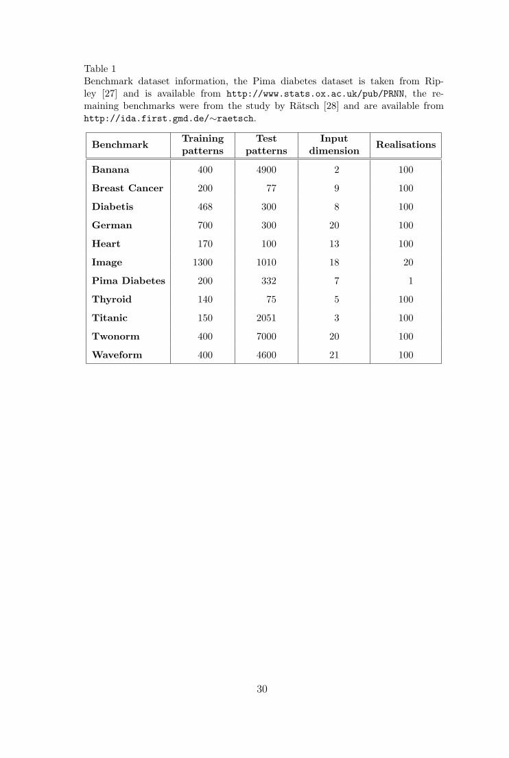
Table 1Benchmark dataset information, the Pima diabetes dataset is taken from Rip-ley [27] and is available from http://www.stats.ox.ac.uk/pub/PRNN, the re-maining benchmarks were from the study by Ratsch [28] and are available fromhttp://ida.first.gmd.de/∼raetsch.

BenchmarkTrainingpatterns

Testpatterns

Inputdimension

Realisations

Banana 400 4900 2 100

Breast Cancer 200 77 9 100

Diabetis 468 300 8 100

German 700 300 20 100

Heart 170 100 13 100

Image 1300 1010 18 20

Pima Diabetes 200 332 7 1

Thyroid 140 75 5 100

Titanic 150 2051 3 100

Twonorm 400 7000 20 100

Waveform 400 4600 21 100

30

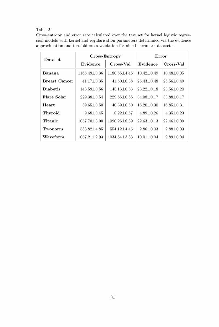
Table 2Cross-entropy and error rate calculated over the test set for kernel logistic regres-sion models with kernel and regularisation parameters determined via the evidenceapproximation and ten-fold cross-validation for nine benchmark datasets.

DatasetCross-Entropy Error

Evidence Cross-Val Evidence Cross-Val

Banana 1168.49±0.36 1180.85±4.46 10.42±0.49 10.48±0.05

Breast Cancer 41.17±0.35 41.50±0.38 26.43±0.48 25.56±0.49

Diabetis 143.59±0.56 145.13±0.83 23.22±0.18 23.56±0.20

Flare Solar 229.38±0.54 229.65±0.66 34.08±0.17 33.88±0.17

Heart 39.65±0.50 40.39±0.50 16.20±0.30 16.85±0.31

Thyroid 9.68±0.45 8.22±0.57 4.89±0.26 4.35±0.23

Titanic 1057.70±3.00 1090.26±8.39 22.63±0.13 22.46±0.09

Twonorm 533.82±4.85 554.12±4.45 2.86±0.03 2.88±0.03

Waveform 1057.21±2.93 1034.84±3.63 10.01±0.04 9.89±0.04

31

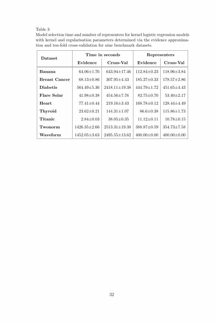
Table 3Model selection time and number of representers for kernel logistic regression modelswith kernel and regularisation parameters determined via the evidence approxima-tion and ten-fold cross-validation for nine benchmark datasets.

DatasetTime in seconds Representers

Evidence Cross-Val Evidence Cross-Val

Banana 64.06±1.76 643.94±17.46 112.84±0.23 118.96±3.84

Breast Cancer 68.13±0.86 307.95±4.43 185.27±0.33 178.57±2.86

Diabetis 564.49±5.36 2418.11±19.38 444.79±1.72 451.65±4.43

Flare Solar 41.98±0.38 454.56±7.76 82.75±0.70 53.40±2.17

Heart 77.41±0.44 219.16±3.43 168.78±0.12 128.44±4.49

Thyroid 23.62±0.21 144.31±1.07 86.6±0.38 115.86±1.73

Titanic 2.84±0.03 38.05±0.35 11.12±0.11 10.78±0.15

Twonorm 1426.35±2.66 2513.31±19.38 388.87±0.59 354.73±7.58

Waveform 1452.05±3.63 2495.55±13.62 400.00±0.00 400.00±0.00

32

Table 4Comparison of sparse Bayesian kernel logistic regression, the support vector machine(SVM) and the relevance vector machine (RVM) over seven benchmark datasets, interms of test set error and the number of representer vectors used. The results forthe SVM and RVM are taken from Tipping [14].

Errors Vectors

Benchmark SVM RVM BKLR SVM RVM BKLR

Pima Diabetis 21.1% 19.6% 21.1% 109.0 4.0 14.0

Banana 10.9% 10.8% 10.9% 135.2 11.4 20.9

Breast Cancer 26.9% 29.9% 27.7% 116.7 6.3 5.5

Titanic 22.1% 23.0% 22.6% 93.7 65.3 7.9

Waveform 10.3% 10.9% 10.2% 146.4 14.6 44.3

German 22.6% 22.2% 22.7% 411.2 12.5 189.3

Image 3.0% 3.9% 4.2% 116.6 34.6 694.0

33