The Ethiopian Commodity Exchange and the coffee … Ethiopian Commodity Exchange and the coffee...

The Ethiopian Commodity Exchange and the coffee market: Are local prices more

integrated to global markets? By Manuel A. Hernandez, Solomon Lemma and Shahidur Rashid,

IFPRI

The Ethiopian Commodity Exchange (ECX) was established in April 2008 with the

objective of improving market efficiency by better linking smallholder farmers to

markets, encouraging reliable trading relationships and increasing market

information. In December 2008 it became mandatory to trade all coffee through the

ECX. This paper examines whether Ethiopian coffee prices have become more

integrated to world prices after the implementation of the ECX. We follow a

multivariate GARCH approach to evaluate the degree of correlation and volatility

transmission across international, auction and producer price returns. We focus on the

five major Ethiopian coffee varieties using monthly data for the period 1992 through

2013. The estimation results indicate that not all coffee regions have necessarily

become more connected to world markets, at least not in the first five years after the

implementation of the mandatory regulation. We also do not find a higher integration

across regional coffee prices.

2

1. Introduction

In the 1990s, several African countries started to implement market-oriented agricultural policies

as part of their development policy framework. Around that time, African economies had

experienced dramatic changes in their export commodity markets, including shocks associated

with price declines, which needed to be addressed (Akiyama, 2001; Gemch and Struthers, 2007;

Rashid et al., 2010). The interventions differed across countries and commodities, but the ultimate

goal remained the same. The policies intended to stabilize producers’ income through marketing

boards that provided a single channel for exports and imports, state ownership of processing

centers, and administration of domestic prices that were normally pan-seasonal, pan-territorial, and

detached from international prices (Akiyama et al. 2003; Gemch and Struthers, 2007). But there

were still institutional and infrastructural challenges in agriculture related to high transaction and

marketing costs, which affected these new policy interventions, compelling economists and

policymakers to turn to other market-based approaches (Deaton, 1999; Gabre-Madhin, 2001). It

was at this stage that African countries became keen on promoting commodity exchanges.

Commodity exchanges are organized markets which serve as a means for risk management

and transaction costs reduction for both buyers and sellers. Historically, commodity exchanges

date back to the middle ages.1 Until recently, commodity exchanges were strictly confined to

industrialized countries, but with the advent of affordable technology many developing countries

in Africa have been keen on establishing one. The wave began in the 1990s, starting with Zambia

and Zimbabwe and followed by Kenya and Uganda (see Table A.1 in the Appendix). The most

recent one to join the group of exchanges in Africa was the Ethiopian Commodity Exchange

established in 2008.

Agricultural markets in Ethiopia have long been exposed to high transaction costs, price

fluctuations and excessive risk (Gabre-Madhin, 2006; Gemech and Struthers, 2007; Rashid et al.,

2010). With only one third of the output reaching the market, commodity buyers and sellers tend

to trade only with the people they know to avoid the possibility of default or being cheated (Gabre-

Madhin, 2001). Small-scale farmers, who produce 95 percent of Ethiopia’s agricultural output,

also have limited access to market information (Worako et al., 2008). Often, smallholders only

1 The first exchange was established in the sixteenth century in England, followed by the Berlin Grain Exchange in

Germany established around the 1840s and the Chicago Stock Exchange in the United States in 1848 (Forrester, 1931;

Hirschstein, 1931).

3

have access to local price information, being unable to negotiate better prices and subject to the

potential market power exerted by local merchants. If farmers in a particular region are especially

productive, their local market becomes glutted and prices drop precipitously. In addition, local

producers often receive a small share of the export price, particularly in the coffee market; this is

largely explained by the participation of several intermediaries along the value chain resulting in

market inefficiencies (Akiyama et al., 2001; Gabre-Madhin, 2006).

To curb the situation, the government of Ethiopia together with its development partners

(The World Bank, International Monetary Fund, Oxfam GB, among others) launched the Ethiopian

Commodity Exchange (ECX) with the aim of creating an efficient, transparent and orderly

marketing system to serve the needs of buyers, sellers and intermediaries, and promote increased

market participation of Ethiopian small-scale producers. It further envisioned creating a

centralized trading floor for buyers and sellers. The new system anticipated to develop more secure

and reliable schemes for handling, grading, storing, among other services, encourage risk-free

payments, and offer a goods delivery system to settle transactions (Gabre-Madhin, 2006; Alemu

amd Meijerink, 2010). It also intended to build trust and transparency among all market actors

through the dissemination of market information and clearly defined rules for trading and

warehousing, as well as the eventual provision of internal dispute settlement services.

In this study, we focus on examining whether Ethiopian coffee prices have become more

integrated to world prices after the implementation of the ECX. We base our analysis on the coffee

sector because coffee is a major export commodity and an important source of employment in

Ethiopia. Coffee is also the most traded agricultural commodity in the ECX both in terms of

volume and value, and significant reforms have occurred in the coffee sector in the past years. We

are particularly interested in examining whether the institutional changes resulting from the

implementation of the ECX have better linked local producers to global markets in terms of higher

price interrelationships. Certainly, a higher price interdependence between domestic and

international prices may signal that part of the objectives of the ECX are being achieved in terms

of stronger linkages with external markets and improved market information, but does not

necessarily mean that it is a welfare-improvement system, particularly among the most vulnerable

groups of farmers. Higher volatility interactions from international to local prices may also have

serious implications for farmers and low-income consumers by making them more vulnerable to

international shocks.

4

We follow a multivariate GARCH (MGARCH) approach, which permits us to better assess

the potential dynamic relationship between local and international coffee markets by formally

accounting for market interactions in terms of the conditional second moment. In particular, we

implement a dynamic model of conditional volatilities in price returns that allows us to evaluate if

the degree of interdependence between markets, measured through time-varying conditional

correlations, has intensified after the establishment of the ECX. Similarly, we explore volatility

transmission across markets and whether volatility spillovers from international to domestic

markets have increased in recent years. We also test for structural changes in the dynamics of local

coffee prices. The study focuses on the five major coffee varieties in Ethiopia using monthly data

for the period 1992 through 2013. The use of monthly data further allows us to capture price

dynamics that would otherwise be hidden in lower frequency data.

The remainder of the paper is organized as follows. Section 2 provides further details about

the coffee market in Ethiopia and the ECX. Section 3 presents the methodological approach used

in the study. Section 4 describes the data and Section 5 reports and discusses the estimation results.

Section 6 concludes.

2. Background

Ethiopia is one of the largest coffee producers in Africa and ranks fifth in the world after Brazil,

Vietnam, Colombia and Indonesia.2 According to the Ministry of Trade (MoT) of Ethiopia, the

country produced an average of 300 thousand tons of coffee per year between 2000 through 2012.

Oromiya and SNNP (Southern Nations Nationality Peoples) are the two major coffee producing

regions, which together roughly account for 97 percent of the total national production as shown

in Table 1. Ethiopia also grows a wide variety of coffee. The south-west part of the country, which

covers Illubabor, Kelem, Jimma, Kaffa, Shaka, Bench Maji and Wollega (Lekemt), produces dry

coffee and represents about 70 percent of the total production. The southern region, which includes

Sidama, Yirgachefe and Wolayeta, produces washed coffee beans and represents 22 percent of the

total production. The eastern coffee growing region, which includes West and East Hararghe

(Harar), produces both dry and washed coffee beans and account for the remaining 8 percent of

the national production. Figure A.1 in the Appendix presents a map with all growing areas of

2 International Coffee Organization (2013), http://www.ico.org.

http://www.ico.org/

5

Arabica coffee in Ethiopia, distinguishing by volume of production, and indicates the five regions

focused in the study.

[Insert Table 1]

In terms of exports, Ethiopia is the highest exporter in Africa and is among the top 10

exporters in the world after Mexico.3 According to the National Bank of Ethiopia (NBE), the

annual average volume of coffee exports was 160 thousand tons between 2000 and 2012, and the

highest volume of exports was registered in 2012 (192 thousand tons). Besides, coffee is a major

source of foreign exchange inflows, constituting about 35 percent of total export earnings. It is

also estimated that 95 percent of the total coffee output is produced by small-scale producers and

the remaining 5 percent by cooperatives and private commercial farmers (Worako et al., 2008).

This reflects the importance of the sector in improving the livelihood of the poor and contributing

to the overall economic growth of the country.

Given the importance of the coffee sector to the economy, the sector has also been exposed

to a wide set of different policies over the past three major regimes: monarchic regime (prior 1974),

central planning regime (1974 to 1991) and Ethiopian People’s Republic Democratic Front

(EPDRF) regime (1991 to present). The substantial policy changes across regimes resulted in

significant changes in the marketing channels, licensing and price setting, which affected the

development of the coffee sector. The market-oriented reforms that started in 1991 aimed at

opening the Ethiopian domestic and export coffee markets with more competitive prices as means

of stimulating farmers’ productivity and growth. However, despite efforts, the performance of the

coffee sector still remains lagging. Poorly instituted modes of production (Zewdu et al., 2010),

high marketing costs (Rashid et al. 2010), volatile prices (Gemech and Struthers, 2007), inadequate

market infrastructure (Rashid et al 2010, Gabre-Madhin, 2009), and an unorganized commodity

marketing approach (Gabre-Madhin, 2009; Gemech and Struthers, 2007) are indicators of market

inefficiency that significantly limit coffee growers’ share from the value of exports and total

earnings from the sector.

3 International Coffee Organization (2013), http://www.ico.org.

http://www.ico.org/

6

2.1. The Ethiopian Commodity Exchange (ECX)

To resolve market inefficiencies, particularly concerning prices along the agricultural marketing

channel, a landmark proclamation was issued by the parliament in 2007 that paved the way for the

establishment of the ECX under the supervision of the Ministry of Agriculture and Rural

Development (MoARD) in Proclamation No-551/2007. The ECX was finally established in April

2008 with the aim of filling the gap created by missing institutions and infrastructure in agricultural

commodity markets (Gabre-Madhin, 2001).4 The objective of the commodity exchange was to

perform four basic functions: (i) reduce transaction costs, (ii) ensure price transparency and price

discovery by creating a secure and reliable system for handling, grading and storing services for

commodity transactions, (iii) promote risk-free payments, and (iv) provide a goods delivery system

to settle transactions (Gabre-Madhin, 2006; Alemu and Meijerink, 2010).

While the commodity exchange initially focused on trading maize, wheat and beans, it

eventually included other commodities such as coffee, sesame and haricot bean (Rashid et al.,

2010). In the case of coffee, in December 2008 it became mandatory to trade all coffee through

the ECX. The volume of coffee traded through the ECX also rapidly increased in the following

years; from about 64 thousand tons in the crop year of 2008/09 to more than 200 thousand tons in

2010/11, representing around 47 percent of the total volume of transactions of the ECX (Gabre-

Madhin, 2012). This rapid transaction growth could be attributed to the measures incorporated by

the ECX to ensure the security of the transactions for its stakeholders. In the new system, trading

through the ECX guarantees a trade day plus one payment schedule for agents, which reduced

information asymmetries and boosted confidence among agents. To stimulate market

transparency, the ECX also started to use several mechanisms to facilitate the disclosure of market

information. Besides using the radio, television and print media to disseminate price information

to farmers, the ECX started to rely on new information and communication technologies (ICTs);

for example, displaying real time price information through electronic ticker boards located in 32

rural sites, instant messaging through mobile phones to more than 250,000 subscribers and

providing website access to more than 107 countries (Gabre-Madhin, 2012).5 In sum, the priorities

4 The budget allocated by the international community for the first phase of the ECX (period 2008-2013) was around

10 million US dollars.

5 The adoption of mobile technology and internet is on surge in Ethiopia due to major recent developments in mobile

phone and internet service provision. Subscription per 100 people for mobile phones and internet has grown from 1.1

7

of the ECX include providing accurate market information to all the market participants and

increase trust among buyers and sellers.

We now turn to formally examine whether local coffee prices become more integrated to

the world market after the implementation of the ECX. We focus on the level of interdependence

and volatility transmission between producer, auction and international price returns.

3. Methodology

This section briefly describes the two MGARCH models used to separately analyze the degree of

interdependence (conditional correlations) and volatility dynamics between producer, auction and

international prices for different major Ethiopian coffee varieties. In particular, we use a DCC and

BEKK model. The DCC model, developed by Engle (2002), is suitable to identify if the degree of

interdependence across the marketing channel for each variety of coffee has changed over time

based on time-varying conditional correlations. The BEKK model, proposed by Engle and Kroner

(1995), is suitable to characterize volatility transmission across markets since it is flexible enough

to account for own- and cross-volatility spillovers and persistence.6 We are particularly interested

in the transmission of volatility from international to domestic markets.

Consider the following vector stochastic process of price returns for each variety of coffee

analyzed,

),,0(~|

,

1

1

0

ttt

t

p

j

jtjt

HIe

err

(1)

where tr is a 3x1 vector of farm gate, auction and international price returns; 0 is a 3x1 vector of

long-term drifts; j , j=1,..,p, are 3x3 matrices of parameters; and te is a 3x1 vector of forecast

errors for the best linear predictor of tr , conditional on past information denoted by 1tI , and with

a corresponding variance-covariance matrix tH . Similar to a standard VAR model, the elements

to 22.4 and from 0.1 to 1.5, respectively, between 2005 and 2012 (World Develolpment Indicators, The World Bank,

http://data.worldbank.org/data-catalog/world-development-indicators).

6 See Bauwens et al. (2006) and Silvennoinen and Teräsvirta (2009) for an overview of different MGARCH models.

http://data.worldbank.org/data-catalog/world-development-indicators

8

of j , j=1,…, p, provide direct measures of own and cross lead-lag relationships at the mean level

between markets.7

In the DCC model, the degree of volatility interdependence between markets is assumed to

be time-dependent across time and is captured through a conditional correlation matrix ),( ,tijtR

3,...,1, ji . The conditional variance-covariance matrix tH is defined as

tttt DRDH (2)

where )...( 2/1

,33

2/1

,11 ttt hhdiagD ; tiih , is a GARCH(1,1) specification, i.e. 1,

2

1, tiiitiiiiit heh ,

i=1,…,3; )()( 2/1

,

2/1

,

tiittiit qdiagQqdiagR ; ,3,...,1,),( , jiqQ tijt is a 3x3 symmetric positive-

definite matrix given by 1

'

11)1( tttt QuuQQ ; and iititit heu . Q is the 3x3

unconditional variance matrix of tu , and and are non-negative adjustment parameters

satisfying 1 . The unconditional variance matrix tQ could be seen as an autoregressive

moving average (ARMA) type process capturing short-term deviations in the correlation around

its long-run level.

In the BEKK model, the conditional variance-covariance matrix tH with one time lag is

given by

,''' 1

'

11 GHGAeeACCH tttt (3)

where C is a 3x3 upper triangular matrix of constants ijc , A is a 3x3 matrix of elements ija that

capture the degree of innovation from market i to market j , and G is a 3x3 matrix of elements

ijg that measure the persistence in conditional volatility between markets i and j . This

specification allows us to analyze the magnitude and persistence of volatility transmission across

7 We checked for cointegration between producer, auction and international log prices and did not find cointegrating

relationships based on the Johansen test. Hence, the VAR specification defined in equation (1) adequately captures

the dynamics of the price returns used in the analysis.

9

the markets under analysis. We can derive impulse-response functions for the estimated

conditional volatilities to show, for example, how a shock in international markets may affect local

auction and producer markets.

4. Data

The data used for the analysis are monthly average producer, auction and international prices for

the period January 1992 through June 2013. The producer and auction price data include the five

major Ethiopian coffee varieties by origin of growing regions namely: Sidama, Yirgachefe, Harar,

Lekemt and Jimma. Sidama and Yirgachefe are part of the Oromiya producing region while Harar,

Lekemt and Jimma are part of the SNNP producing region. The five varieties constitute about 95

percent of the total coffee produced and exported in the country.8

Unlike many coffee growing countries, Ethiopian coffee varieties are often differentiated by

agro-ecological and local conditions, shape, acidity, body, flavor, aroma and processing method,

and they are generally auctioned by their corresponding origin. In particular, Ethiopian coffee is

traded in the world market based on their origin of production (e.g., Sidama, Yirgachefe, Harar,

Jimma, Lekemt, Teppi, Limu and Bebeka). Recently, Ethiopia also secured exclusive trademark

rights for Sidama, Yirgachefe and Harar coffee, which serves to further highlight the differences

between Ethiopian coffee types.9 It is worth then examining the degree of interdependence and

volatility transmission between international and domestic markets for different coffee varieties in

Ethiopia.

Producer prices were obtained from the monthly published producer price survey reports of

the Central Statistical Agency (CSA) of Ethiopia.10 Auction prices were obtained from the

Agricultural Market Promotion Department (AMPD) of MoARD for the period January 1992 to

December 2008 and directly from the Ethiopian Commodity Exchange (ECX) for the following

8 According to the Ethiopian Coffee Authority, in 2011 Sidama accounted for 41% (65,470 bags) of the total country

exports; Jimma for 21% (33,476 bags), Lekempti for 17% (26,128 bags), Harar for 9% (13,697 bags), and Yirgachefe

for 6% (9,914 bags).

9 Ethiopia owns trademark rights for the distinctive fine coffee of Sidamo, Yirgacefe and Harar brands since 2008.

10 The CSA conducts monthly surveys and release monthly reports since 1981. Monthly Bulletins No. 44 to 450 were

used to compile the producer price data.

10

years.11 The international price is the New York Arabica coffee price indicator calculated by the

International Coffee Organization (ICO) on the basis of different Arabica coffees traded.12

The sample period covered allows us to evaluate if there have been important changes in the

degree of interdependence and dynamics of volatility before and after the mandatory regulation of

trading and exporting coffee through the ECX, which became effective in January 2009. All prices

in the analysis are standardized to US cents per pound.

Figure 1 shows the evolution of the international price and the producer and auction price

for the five coffee varieties. We observe that international and local prices, particularly auction

prices, generally co-move in all five markets. The important spikes in the international price of

coffee in 1994 and 2011, due to weather-related supply disruptions in Brazil and Colombia, are

also observed in the auction price across all five coffee varieties; the international price spike of

1997, also due to supply shortages, is only observed in the auction price in Yirgachefe. Producer

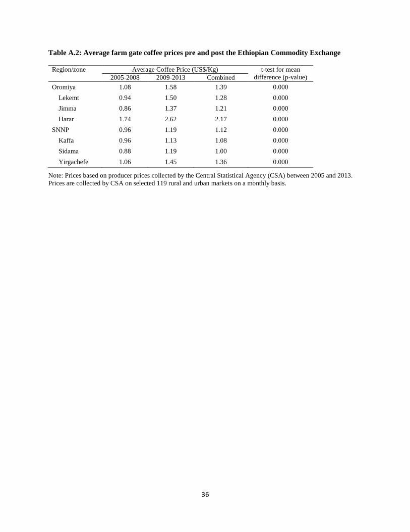
prices in all five markets, in turn, only exhibit an important spike in 2011. Table A.2 in the

Appendix also compares producer coffee prices collected in monthly surveys by CSA, before and

after the implementation of the implementation of the ECX, and shows that prices in all local

markets have increased in recent years.

[Insert Figure 1]

Figure 2 plots the corresponding price returns (in percentage points). The price returns are

defined as 1ln ttt ppr , where tp is the producer, auction or international price at time t. This

logarithmic transformation is generally used in empirical finance as a standard measure for net

returns in a market, which also provides a convenient support for the distribution of the error terms

in the estimated models. Two patterns emerge from this figure. First, all price returns exhibit

important fluctuations across time, which is indicative of time-varying volatility in returns and

motivates the use of MGARCH models. Second, the fluctuations in price returns decrease as we

move from producer to auction and international markets; i.e., the returns in international markets

11 Prior to 2009, the AMPD kept record in monthly (unpublished) bulletins of the average prices paid to suppliers at

the Coffee Auction Market (CAM).

12 We also considered the Brazilian Naturals price indicator as another relevant approximation of the international

price for the Ethiopian coffee and find qualitatively similar results. The Brazilian Naturals price indicator is the

combination of ex-dock prices in New York and Germany of a group of traditional exporting coffee countries

including Ethiopia. The correlation between the New York and Brazilian Naturals prices is 0.987.

11

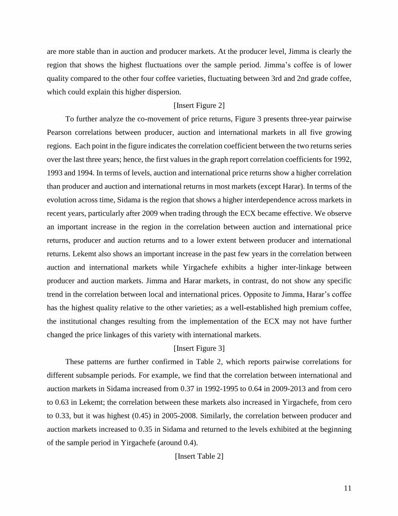
are more stable than in auction and producer markets. At the producer level, Jimma is clearly the

region that shows the highest fluctuations over the sample period. Jimma’s coffee is of lower

quality compared to the other four coffee varieties, fluctuating between 3rd and 2nd grade coffee,

which could explain this higher dispersion.

[Insert Figure 2]

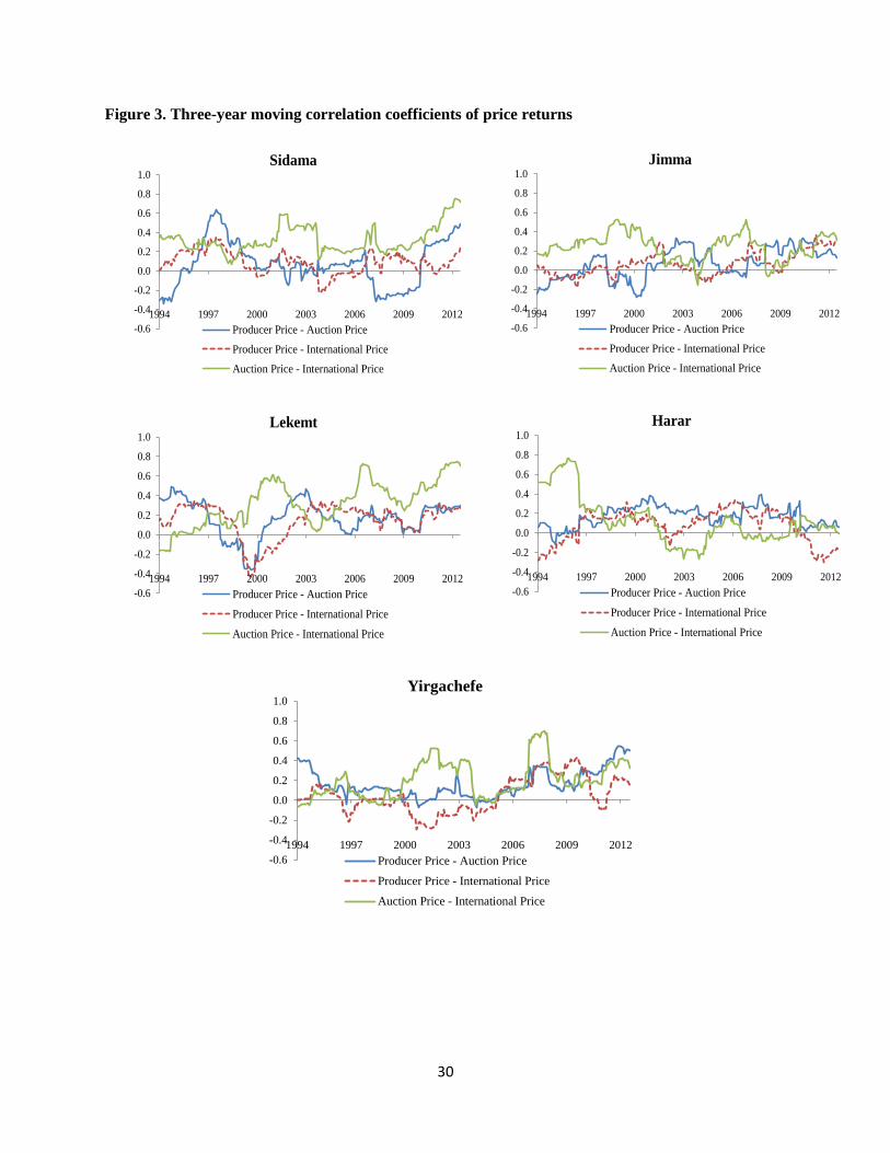
To further analyze the co-movement of price returns, Figure 3 presents three-year pairwise

Pearson correlations between producer, auction and international markets in all five growing

regions. Each point in the figure indicates the correlation coefficient between the two returns series

over the last three years; hence, the first values in the graph report correlation coefficients for 1992,

1993 and 1994. In terms of levels, auction and international price returns show a higher correlation

than producer and auction and international returns in most markets (except Harar). In terms of the

evolution across time, Sidama is the region that shows a higher interdependence across markets in

recent years, particularly after 2009 when trading through the ECX became effective. We observe

an important increase in the region in the correlation between auction and international price

returns, producer and auction returns and to a lower extent between producer and international

returns. Lekemt also shows an important increase in the past few years in the correlation between

auction and international markets while Yirgachefe exhibits a higher inter-linkage between

producer and auction markets. Jimma and Harar markets, in contrast, do not show any specific

trend in the correlation between local and international prices. Opposite to Jimma, Harar’s coffee

has the highest quality relative to the other varieties; as a well-established high premium coffee,

the institutional changes resulting from the implementation of the ECX may not have further

changed the price linkages of this variety with international markets.

[Insert Figure 3]

These patterns are further confirmed in Table 2, which reports pairwise correlations for

different subsample periods. For example, we find that the correlation between international and

auction markets in Sidama increased from 0.37 in 1992-1995 to 0.64 in 2009-2013 and from cero

to 0.63 in Lekemt; the correlation between these markets also increased in Yirgachefe, from cero

to 0.33, but it was highest (0.45) in 2005-2008. Similarly, the correlation between producer and

auction markets increased to 0.35 in Sidama and returned to the levels exhibited at the beginning

of the sample period in Yirgachefe (around 0.4).

[Insert Table 2]

12

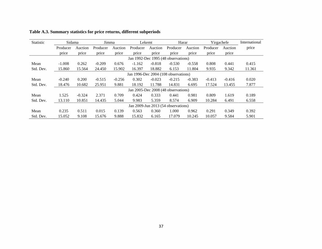
Finally, Table 3 reports summary statistics of all returns series. We observe that the returns

in the international market are on average higher than in the auction and producer markets. In

particular, the average monthly return in the international market is 0.2%, which is only exceeded

by the average return in the auction market in Yirgachefe (0.28%). Yirgachefe is also the region

that together with Jimma exhibit the highest return in the producer market (0.19%), although

Jimma shows a much higher dispersion. We also note that the returns are on average higher in

auction than producer markets in Sidama, Harar and Yirgachefe.13 As noted above, producer

returns show a higher variation (standard deviation) than the returns in the other markets; in

particular, they exhibit between 1.2 and 2.1 times more dispersion than auction returns and

between 1.6 and 2.7 times more dispersion than international returns.

[Insert Table 3]

In addition, the Jarque-Bera test reveals that all returns series seem to follow a non-normal

distribution. The kurtosis is greater than three in all series, pointing to a leptokurtic distribution of

returns and motivating the use of a Student’s t density in the estimation of the DCC and BEKK

models (hereafter T-DCC and T-BEKK). The Ljung-Box (LB) for up to 6 and 12 lags generally

reject the null hypothesis of no autocorrelation for the squared returns in most markets, which

further motivates the use of MGARCH models given the apparent non-linear dependencies in

returns. Lastly, the Augmented Dickey-Fuller (ADF) and Kwiatkowski-Phillips-Schmidt-Shin

(KPSS) tests confirm the stationarity of the returns series.

5. Results

This section presents the results of the MGARCH models estimated to examine the level of

interdependence and volatility transmission between international, auction and producer price

returns for five different varieties of Ethiopian coffee. We first focus on the estimation results of

the T-DCC model, which allows us to identify if the degree of interdependence (conditional

correlations) between markets has changed across time. We then discuss the results of the T-BEKK

model, which permits us to characterize volatility transmission from international to domestic

13 When segmenting the sample, we find that producer and auction price returns seem to have increased across time

in most of the analyzed coffee markets, as opposed to the price returns in the international market. As shown in Table

A.3, in the 90s and early 2000s the average returns in several of the markets were negative. Yet, we start to observe

higher average returns from 2005 and not necessarily after the implementation of the ECX in December 2008.

13

markets both before and after the mandatory regulation of trading and exporting all coffee through

the ECX. We further test whether the change in the regulation in December 2008 was accompanied

by a structural break in the mean and volatility of the analyzed price return series.

5.1. Market interdependence

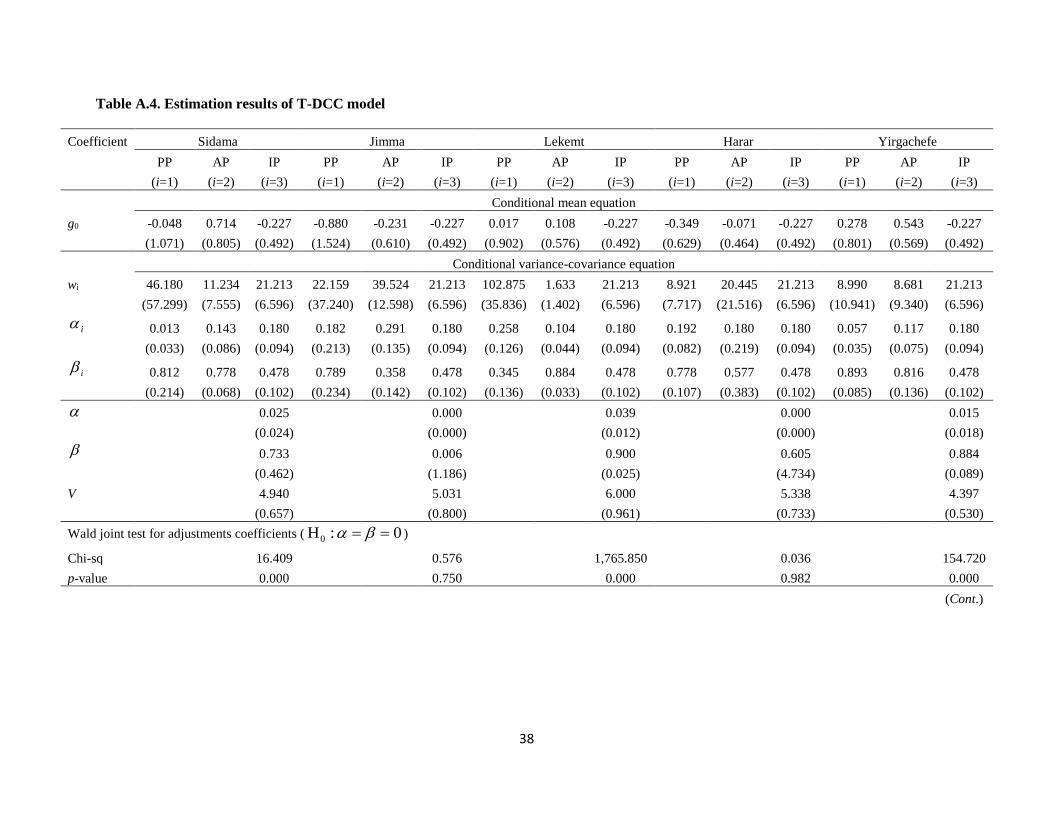
Table A.4 presents the estimation results of the T-DCC model. The upper panel reports the

estimated coefficients of the conditional mean equation and the lower panel reports the coefficients

of the conditional variance-covariance matrix defined in equation (2). The estimated degrees of

freedom parameter (v) is relatively small in all cases, ranging between 4 and 6, which supports the

adequacy of the estimations using a Student’s t distribution. The residual diagnostic tests, reported

at the bottom of the table, also support the appropriateness of the model specification. The Ljung-

Box (LB), Lagrange Multiplier (LM) and Hosking Multivariate Pormanteau (M) tests statistics for

6 and 12 lags generally show no or weak evidence of autocorrelation, ARCH effects and cross-

correlation in the standardized model residuals.

In terms of interactions at the mean level, we do not find any own and cross lead-lag

relationships in the return series analyzed in each of the five regions. The Schwarz’s Bayesian

information criterion (SBIC) indicates that the expected price returns in a certain month do not

depend on their past values and are also not affected by past returns in the other markets. Hence,

lagged local and international price returns do not seem to affect current local price returns at the

mean level.

Turning to the conditional variance-covariance equation, however, we do find time-varying

conditional correlations between international and domestic price returns in some regions. In

particular, the Wald test rejects the null hypothesis that the adjustment parameters and are

jointly equal to zero with a 95 percent confidence level in Sidama, Lekemt and Yirgachefe. In

Jimma and Harar, in turn, these correlations seem to have remained constant over the entire period

of analysis.

To appreciate the evolution of the correlations over time, Figure 4 presents the pairwise

dynamic conditional correlations between producer, auction and international price returns for

14

each growing region, resulting from the T-DCC model estimates.14 Several patterns emerge from

the figures. First, the estimated conditional correlations confirm a higher interdependence between

auction and international markets as compared to producer with auction and international markets.

Second, we observe important fluctuations across time in the correlation between international and

domestic markets, particularly in Lekemt and Sidama, and to a lower extent in Yirgachefe; in

Jimma and Harar, which are the coffee varieties of the lowest and highest quality among the five

varieties, the correlations across markets have remained constant across time. Third, similar to the

preliminary analysis based on unconditional correlations, Lekemt and Sidama show a higher

interdependence between auction and international markets in more recent years. The case of

Lekemt is particularly notable; as shown in Table 4, which reports the average conditional

correlations for different subperiods, the correlation between the auction market in Lekemt and the

international market more than doubled from 0.20 in 1992-1995 to 0.44 in 2009-2013. In Sidama,

this correlation has already been relatively high, fluctuating around 0.42 between 1992 and 2008,

but it further increased to 0.44 after 2008. The auction market in Yirgachefe also shows a higher

interrelation with the international market (as compared to the early 90s), but the increase in the

correlation occurred prior to 2009.

[Insert Figure 4]

[Insert Table 4]

The correlation between producer and auction markets in Sidama also exhibits an important

increase after 2008, although the level of interdependence between these markets (0.09) is still not

as strong as in Yirgachefe, Harar and Lekemt (0.18-0.27). In both Lekemt and Yirgachefe,

however, the degree of correlation between producer and auction price returns is lower in recent

years than in the early 90s. Finally, international and producer markets in Sidama, Lekemt and

Yirgachefe also appear to have become more interconnected during the last decade, but the

increase in the correlation did not necessarily occurred after 2008 when the regulation of trading

and exporting all coffee through the ECX became effective.

Despite some differences in the evolution of the correlations between local and

international prices across different coffee varieties, the existence of the Coffee Auction Market

14 The figure also includes constant conditional correlations and one standard deviation confidence bands based on

Bollerslev’s (1990) Constant Conditional Correlation (CCC) model.

15

(CAM) prior to the ECX could generally explain the relatively high correlation between

international and auction prices and the lack of further significant increases in the correlation

between international and several domestic coffee prices after 2008. The CAM was established by

the Ethiopian government in 1992 as part of the liberalization of the domestic coffee marketing

system. Thus, some markets could already have been more connected to world markets, and it

would probably take a couple more years to observe the full effects of the ECX in terms of further

linking local coffee producers to global markets. Note also that while market (price) transparency

has further increased with the implementation of the ECX (favoring a higher correlation between

domestic and international prices), direct trade agreements between exporters and local coffee

producers have disappeared (favoring a lower correlation between domestic and international

prices).

As an additional analysis, we examine whether local Ethiopian coffee markets have

become more integrated at the producer and auction level in recent years. We estimate two separate

T-DCC models, one model including the five producer price returns series (corresponding to the

five coffee varieties) and a second model including the five auction price returns series. The full

estimations results are reported in Table A.5 while Figure A.2 presents the estimated pairwise

conditional correlations for different subsample periods. Two patterns are worth remarking from

the figure. First, markets are more integrated at the auction than at the producer level; except for

Lekemt and Harar, the conditional correlations between markets at the auction level are higher and

in most cases more than double the conditional correlations at the producer level. Second, markets

in Ethiopia both at the producer and auction stage have not necessarily become more integrated

after the implementation of the EXC.

5.2. Volatility transmission

We now turn to examine the cross-volatility dynamics from international to domestic price returns

based on the estimation results of the T-BEKK model. Since we are interested in analyzing

volatility interactions between international and domestic markets before and after the mandatory

regulation of trading all coffee through the ECX, we estimate the model over two subperiods: 1992

through 2008 and 2009 through 2013. Tables A.6 and A.7 present the corresponding results with

16

the estimated coefficients of the conditional variance-covariance matrix defined in equation (3).15

As in the T-DCC model, the estimated degrees of freedom parameter (v) supports the adequacy of

the estimation with a Student’s t distribution and the reported diagnostic tests for the standardized

squared residuals (LB, LM and M statistics) generally support the appropriateness of the model

specification.

The diagonal iia coefficients, 3,...,1i , capture own-volatility spillovers (the effect of own

lagged shocks on the current conditional return volatility in market i), while the diagonal iig

coefficients capture own-volatility persistence (the dependence of volatility in market i on its own

past volatility). The off-diagonal coefficients ija and ijg measure, in turn, direct spillover and

persistence effects from market i to market j. The Wald joint test for cross-volatility rejects the

null hypothesis that the off-diagonal coefficients ija and ijg are jointly equal to zero, indicating

that there are cross spillovers and persistence effects across markets.

To examine volatility spillovers between specific markets, in our case from international to

domestic markets, it is important to account for both direct and indirect cross effects. This is

because markets may be directly related through the conditional variance and indirectly related

through the conditional covariance.16 Following Gardebroek and Hernandez (2013) and Hernandez

et al. (2014), we derive impulse-response functions, which control for both direct and indirect

effects, to simulate how a shock in the (conditional) volatility of price returns in the international

market will transmit to the volatility of price returns in the producer and auction markets.

Figure 5 presents the impulse-response functions resulting from a shock equivalent to a 1%

increase in the own conditional volatility of the international market. The responses in each market

are normalized by the size of the original shock. Two patterns are worth noting. First, it is clear

that there is a higher volatility transmission from international to auction markets than to producer

markets, but these spillover effects have not generally intensified after 2008. In Sidama and

Lekemt, for example, the higher (conditional) correlation in price returns between international

and auction markets observed in recent years is not accompanied by higher volatility spillovers

15 To save space, we do not report the estimated constant terms in the conditional mean equation, which are similar to

the T-DCC estimates.

16 The volatility dynamics across markets ultimately comprises all off-diagonal ija and ijg coefficients.

17

from international to domestic markets; while a shock in the international market had a somewhat

similar initial effect on the conditional volatility of auction returns in these two regions during

1992-2008, the effects after 2008 are much smaller (a 1% increase in volatility in international

markets only results in a 0.2% initial increase in the volatility in auction markets). Second, except

for Jimma, the volatility spillovers from international to producer price returns have either

remained constant or marginally increased after 2008, although these cross effects are still relative

small; in the case of Sidama and Lekemt, a 1% increase in volatility in international markets results

in a 0.2% increase in volatility in producer markets, while in Yergachefe and Harar it only results

in a 0.1% increase in volatility. Hence, the volatility transmission analysis is not conclusive on

whether volatility spillovers from international to domestic markets have intensified after the

mandatory regulation of December 2008.

[Insert Figure 5]

5.3. Structural breaks

As a complementary exercise, we examine if the change in the regulation in the coffee market is

correlated with a structural break in the mean and volatility of the producer and auction returns

series in any of the five growing regions. We want to assess whether the mandatory regulation had

a major impact (break) in the dynamics of price returns in these markets.

We implement the test for the presence of unknown breakpoints developed by Lavielle and

Moulines (2000). This test is suitable for strongly dependent processes such as GARCH processes

as it assumes beta-mixing conditions (Carrasco and Chen, 2002).17 We test for structural breaks

on the mean of the price returns and the square of the price returns as a proxy of volatility.18

Table A.8 reports the identified break dates for each returns series representing major

change-points in both their mean and volatility. We observe important shifts in the mean of the

producer returns of most regions in recent years, as opposed to the shifts in volatility, although the

breaks did not occur right after the change in the regulation. The shifts occurred in December 2010

in Sidama and Lekemt, in April 2011 in Harar and in February 2012 in Yergachefe. Sidama also

17 Bai and Perron’s test, for example, assumes uniform mixing conditions that are not satisfied by series exhibiting

time-varying volatility, which is the case of the series used in the present analysis.

18 The test searches for breaks over a maximum number pre-defined potential segments, and uses a minimum penalized

contrast to identify the breaks. We set the minimum length of a segment as 2 months.

18

shows a shift in volatility around December 2010. The breaks in the auction markets, and naturally

in the international market, are more linked to the global supply shortages of 1994 and 1997.

Hence, it is not clear that the mandatory trading regulation resulted in a breakpoint in the dynamics

of the returns series in the growing regions, at least not immediately.

Overall, while a simple comparison between local coffee prices before and after the

implementation of the ECX in December 2008 reveal that local prices have increased (see Table

A.2), our estimation results suggest that the mandatory regulation of trading all coffee through the

ECX has not necessarily promoted a higher integration of all Ethiopian regional coffee prices to

world prices. Only Sidama and Lekemt show a higher interdependence, measured through

conditional correlations, between local (mainly auction markets) and international markets. Yet,

the correlation between producer (farm gate) and international markets is still low. In addition.

Ethiopian local markets do not seem to have become more integrated in recent years. We also do

not find major volatility spillovers from international to local markets in recent years. The

breakpoint analysis further do not suggests structural breaks in the dynamics of the producer and

auction return series around the implementation of the mandatory regulation.

6. Concluding remarks

This paper has examined the degree of interdependence and volatility transmission between

international and domestic price returns to assess whether Ethiopian coffee prices have become

more integrated to world prices in recent years, particularly after the implementation of the ECX

in December 2008. We focus on monthly prices of the five major coffee varieties in Ethiopia,

which include Sidama, Jimma, Lekemt, Harar and Yirgachefe. We implement a MGARCH

approach to derive dynamic conditional correlations and evaluate volatility transmission from

international to domestic markets.

The estimation results indicate that not all coffee regions have become more interrelated

with the world markets after the implementation of the ECX. Despite the general increase in

producer coffee prices after 2008, only few regions show a higher interdependence between local

and international price returns. In particular, only Sidama and Lekemt exhibit a higher interrelation

(conditional correlation) between auction and international prices while the correlation between

producer and international prices is still low. We further do not observe a higher price integration

across different local coffee markets. Volatility spillovers from international to domestic prices

19

have also not increased in the past years. Finally, the ECX does not seem to have produced a major

shift in the dynamics of domestic coffee price returns, at least not in the following months after its

implementation.

The lack of a higher integration between local and world markets in recent years, measured

through interdependencies in prices, could be explained by several factors. First, there have only

been a few years since the ECX was established such that the process of better linking farmers to

markets, encouraging reliable trading relationships, and improving market information is still

ongoing. We observe so far that farmers are receiving higher prices than before the establishment

of the ECX and the volume of coffee transactions through the ECX have considerably increased

in the past years. Second, a coffee auction system (CAM) was already functioning for more than

fifteen years prior to the ECX. This could also explain the absence of further major increases in

the price correlation between international and several domestic coffee varieties, at least in the

short run, as some markets (particularly auction markets) could already have been connected with

global markets although with varying degrees. This is also in line with the lack of structural breaks

in the domestic price series around the implementation of the ECX. Third, there are still additional

bottlenecks across the coffee supply chain that need to be addressed, like lagging production

technologies, lack of infrastructure and, in particular, the higher regulations for the licensing of

traders, that could be limiting the correlation between domestic and international prices. While the

ECX intended to reduce the potential market power exerted by a few major coffee exporters, it has

also eliminated direct trading relationships between exporters and small coffee producers, which

now have to sell their product through still a few licensed traders operating in each region. In

addition, the lack of traceability of the coffee purchased by exporters from specific growing areas

(producers) and the decrease in the predictableness of particular coffee stocks and corresponding

price movements (that allow exporters to mitigate price risks) could also be limiting the local-

international price correlation, despite the higher aggregate (regional) price information.

Future research should continue to study the evolution of the price interrelationship

between international and local coffee markets, especially at the producer level, and assess the

effects of an eventual higher international dependence (if any) of local producers. A higher

integration between local and international markets in the medium- and long-term, which is in line

with the objectives of the ECX, does not certainly mean that the welfare of local coffee producers

will increase and vice versa. For example, higher price volatility transmission from international

20

to local markets could make small-scale farmers and low-income consumers more vulnerable to

international price shocks, particularly in the absence of efficient risk sharing mechanisms.

Policies to address potential periods of excessive price volatility in the future should also need to

pay greater attention to external sources of variation.

21

References

Akiyama, T. Baffes, J. Larson, D., Varangis, P., 2001. Commodity market reforms: Lessons of

Two Decades. The World Bank, Washington, DC.

Akiyama, T. Baffes, J. Larson, D., Varangis, P., 2003. Commodity market reform in Africa: Some

Recent Experience. World Bank Policy Research Working Paper 2995, Washington, DC.

Alemu, D., Meijerink, G., 2010. The Ethiopian Commodity Exchange: An overview. Wageningen

University, The Netherlands.

Bauwens, L., Laurent, S., Rombouts, J.V.K., 2006. Multivariate GARCH models: A survey.

Journal of Applied Econometrics 21, 79-109.

Bollerslev, T., 1990. Modeling the coherence in short-run nominal exchange rates: a multivariate

generalized ARCH model. Review of Economics and Statistics 72, 498-505.

Carrasco, M., Chen, X., 2002. Mixing and moment properties of various Garch and stochastic

volatility models. Econometric Theory 18, 17-39.

Deaton, A., 1999. Commodity Prices and Growth in Africa. Journal of Economic Perspectives 13,

23-40.

Engle, R., 2002. Dynamic conditional correlation-a simple class of multivariate GARCH models.

Journal of Business and Economic Statistics 20, 339-350.

Engle, R., Kroner, F.K., 1995. Multivariate simultaneous generalized ARCH. Econometric Theory

11, 122-150.

Forrester, R.B., 1931. Commodity Exchanges in England. Annals of the American Academy of

Political and Social Science 151, 196-207.

Gabre-Madhin, E.Z., 2001. Market Institutions, Transaction Costs, and Social Capital in the

Ethiopian Grain Market. Research Report 124. International Food Policy Research Institute,

Washington, DC.

Gabre-Madhin, E.Z, 2006. Building Institutions for Markets: The Challenge in the Age of

Globalization. Paper presented at the Employment, Growth and Development Initiative

(EGDI) Policy, Poverty and Agricultural Development in Sub-Saharan Africa Workshop,

Frösundavik, Sweden.

Gabre-Madhin, E.Z, 2009. A Market for all Farmers: Market Institution and Smallholder

Participation. Agriculture for Development paper No AfD-0903. Issued July.

Gabre-Madhin, E. 2012. A Market for Abdu: Creating a commodity Exchange in Ethiopia.

International Food Policy Research Institute, Washington, DC.

22

Gardebroek, C., Hernandez, M.A., 2013. Do energy prices stimulate food price volatility?

Examining volatility transmission between US oil, ethanol and corn market. Energy

Economics 40, 119-129.

Gemech, F., Struthers, J., 2007. Coffee Price Volatility in Ethiopia: Effects of market reform

programs. Journal of International Development 19, 1131-1142.

Hernandez, M.A., Ibarra, R., Trupkin, D.R., 2014. How far do shocks move across borders?

Examining volatility transmission in major agricultural futures markets. European Review

of Agricultural Economics 41(2), 301-325.

Hirschstein, H., 1931. Commodity Exchanges in Germany. Annals of the American Academy of

Political and Social Science 151, 208-217.

Lavielle, M., Moulines, E., 2000. Least-squares estimation of an unknown number of shifts in a

time series. Journal of Time Series Analysis 21, 33–59.

Silvennoinen, A., Teräsvirta, T., 2009. Multivariate GARCH models. In: Andersen, T.G., Davis,

R.A., Kreiss, J.P., Mikosch, T. (Eds.), Handbook of Financial Time Series, 201-229.

Springer, Berlin.

Rashid, S., Winter-Nelson, A., Garcia, P., 2010. Purpose and Potential for Commodity Exchanges

in African Economies. IFPRI Discussion Paper No. 01035. International Food Policy

Research Institute, Washington, DC.

Worako, T.K., van Schalkwyk, H.D., Alemu, Z.G., Ayele, G., 2008. Producer price and price

transmission in a deregulated Ethiopian coffee market. Agrekon 47(4), 492-508.

Zewdu, A., Bamlaku A., Alemub, M., 2010 Agricultural Productivity Growth and Poverty

Reduction in Rural Ethiopia. Institute for Land, Water and Society, Charles Sturt University,

WaggaWagga Campus, NSW, Australi 2010.

23

Table 1. Coffee production in Ethiopia by region, 2005-2013

Region

Production Estimate (In thousand tons)

2005-2008 2008-2013 Average

Oromiya 199.7 259.0 229.4

SNNP 113.0 138.1 125.5

Gambella 3.4 2.2 2.8

Total National 316.1 400.5 358.3

Share of total (%)

Oromiya 63.2 64.7 64.0

SNNP 35.7 34.5 35.0

Gambella 1.1 0.5 0.8

Note: Volume of production obtained from Central Statistical Agency (CSA). SNNP=Southern Nations Nationality

Peoples. Of the five main coffee varieties analyzed in the study, Harar, Lekemt and Jimma are part of the Oromiya

production region and Sidama and Yirgachefe are part of the SNNP production region.

24

Table 2. Unconditional correlations of price returns

Price Jan1992-Dec 1995 Jan 1996-Dec 2004 Jan 2005-Dec 2008 Jan 2009-Jun 2013 Full sample

PP AP IP PP AP IP PP AP IP PP AP IP PP AP IP

Sidama

Producer price (PP) 1.000 -0.201 0.044 1.000 0.194* 0.059 1.000 -0.125 0.259 1.000 0.346* 0.126 1.000 0.070 0.089

Auction price (AP) 1.000 0.368* 1.000 0.221* 1.000 0.285* 1.000 0.636* 1.000 0.333*

International price (IP) 1.000 1.000 1.000 1.000 1.000

Jimma

Producer price (PP) 1.000 -0.181 0.004 1.000 0.108 0.051 1.000 -0.020 0.078 1.000 0.207 0.240 1.000 0.021 0.060

Auction price (AP) 1.000 0.216 1.000 0.211* 1.000 0.473* 1.000 0.266 1.000 0.242*


Lekemt

Producer price (PP) 1.000 0.403* 0.194 1.000 0.062 0.099 1.000 0.171 0.207 1.000 0.225 0.198 1.000 0.187* 0.146*

Auction price (AP) 1.000 -0.048 1.000 0.222* 1.000 0.593* 1.000 0.624* 1.000 0.167*


Harar

Producer price (PP) 1.000 0.017 0.101 1.000 0.244* 0.152 1.000 0.242 0.260 1.000 0.083 -0.148 1.000 0.143* 0.038

Auction price (AP) 1.000 0.491* 1.000 0.062 1.000 0.000 1.000 0.057 1.000 0.204*


Yirgachefe

Producer price (PP) 1.000 0.410* 0.021 1.000 0.052 -0.066 1.000 0.267 0.323* 1.000 0.404* 0.150 1.000 0.161* 0.027

Auction price (AP) 1.000 -0.004 1.000 0.095 1.000 0.453* 1.000 0.331* 1.000 0.135*


# obs. 48 108 48 54 258

Note: The correlations reported are the Pearson correlations. The symbol (*) denotes significance at 5% level.

25

Table 3. Summary statistics for price returns

Statistic Sidama Jimma Lekemt Harar Yirgachefe International

Producer Auction Producer Auction Producer Auction Producer Auction Producer Auction price

price price price price price price price price price price

Mean 0.045 0.179 0.190 0.179 0.107 -0.025 0.103 0.119 0.189 0.282 0.203

Median 0.587 0.000 0.299 0.095 -0.461 -0.590 0.080 -0.040 0.000 -0.142 -0.774

Minimum -59.533 -35.786 -73.760 -63.393 -67.481 -70.616 -42.505 -32.306 -59.324 -30.632 -19.066

Maximum 78.392 49.232 87.960 41.654 41.278 67.947 44.558 38.849 48.691 49.506 47.499

Std. Dev. 16.338 11.425 21.901 10.578 16.039 11.676 13.131 8.660 13.653 10.887 8.032

Skewness -0.018 0.388 -0.114 -0.737 -0.462 -0.276 -0.034 0.306 -0.404 0.847 1.168

Kurtosis 5.854 5.867 5.122 8.643 4.802 13.404 4.260 7.539 7.079 6.702 7.406

Jarque-Bera 87.6 94.9 49.0 365.7 44.1 1167.0 17.1 225.5 185.9 178.2 267.4

p-value 0.000 0.000 0.000 0.000 0.000 0.000 0.000 0.000 0.000 0.000 0.000

# obs. 258 258 258 258 258 258 258 258 258 258 258

Returns correlations

AC (lag=1) -0.164* -0.082 -0.253* -0.001 -0.186* -0.158* -0.298* -0.026 -0.067 -0.089 0.177*

AC (lag=2) 0.015* -0.056 -0.106* 0.011 0.028* 0.034* 0.074* -0.005 -0.087 -0.018 0.140*

LB (6) 14.470* 7.477 27.301* 15.871* 11.616 20.505* 32.466* 9.057 7.159 5.952 24.994*

LB (12) 25.736* 15.832 45.358* 22.256* 15.843 30.606* 36.626* 15.596 15.576 21.383* 33.070*

Squared returns correlations

AC (lag=1) 0.049 0.068 0.0792 0.1175 0.183* 0.171* 0.231* 0.074 0.307* 0.193* 0.109

AC (lag=2) -0.053 0.070 0.0610 0.0685 0.214* 0.041* 0.1930* -0.010 0.223* 0.124* 0.262*

LB (6) 3.756 3.398 11.666 36.803* 26.717* 10.625 40.263* 8.218 53.198* 16.109* 22.185*

LB (12) 6.110 11.699 20.471* 37.496* 31.246* 58.279* 53.816* 11.754 55.135* 60.571* 24.453*

Tests for stationarity

ADF (lag=6) -7.096* -6.561* -7.534* -5.744* -7.546* -5.866* -6.869* -7.296* -8.067* -7.235* -5.901 *

KPSS (lag=6) 0.039 0.047 0.043 0.056 0.035 0.060 0.023 0.036 0.039 0.040 0.060

Note: The symbol (*) denotes rejection of the null hypothesis at the 5% significance level. AC is the autocorrelation coefficient; LB is the Ljung-Box

autocorrelation test; ADF is the Augmented Dickey-Fuller test; and KPSS is the Kwiatkowski-Phillips-Schmidt-Shin test for stationarity.

26

Table 4. Average conditional correlations for different subperiods based on T-DCC model

Correlation Jan1992-Dec 1995 Jan 1996-Dec 2004 Jan 2005-Dec 2008 Jan 2009-Jun 2013 Full sample

Sidama

Producer-Auction 0.041 0.080 0.055 0.091 0.070

(0.035) (0.039) (0.025) (0.040) (0.041)

Producer-International 0.042 0.052 0.058 0.054 0.052

(0.037) (0.037) (0.024) (0.026) (0.033)

Auction-International 0.420 0.416 0.420 0.440 0.423

(0.061) (0.035) (0.022) (0.025) (0.039)

Jimma


(0.000) (0.000) (0.000) (0.000) (0.000)


(0.000) (0.000) (0.000) (0.000) (0.000)


(0.000) (0.000) (0.000) (0.000) (0.000)

Lekemt


(0.084) (0.114) (0.037) (0.049) (0.089)


(0.090) (0.111) (0.046) (0.054) (0.088)


(0.101) (0.088) (0.037) (0.069) (0.115)

Harar


(0.000) (0.000) (0.000) (0.000) (0.000)


(0.000) (0.000) (0.000) (0.000) (0.000)


(0.000) (0.000) (0.000) (0.000) (0.000)

Yirgachefe


(0.027) (0.024) (0.021) (0.029) (0.032)


(0.025) (0.025) (0.023) (0.021) (0.030)


(0.027) (0.045) (0.034) (0.023) (0.040)

# obs. 48 107 49 54 258

Note: The conditional correlations are derived from the estimation results of the T-DCC model. Standard deviations

reported in parentheses.

27

Figure 1. Producer, auction and international prices

Note: Producer prices obtained from the Central Statistical Agency (CSA), auction prices from the Ministry of

Agriculture and Rural Development (MoARD) and the Ethiopian Commodity Exchange (ECX, and international

price from the International Coffee Organization (ICO).

0

50

100

150

200

250

300

1992 1996 2000 2004 2008 2012

US

Cen

ts p

er

lb

Sidama

Producer Price Auction Price International Price

0

50

100

150

200

250

300

1992 1996 2000 2004 2008 2012

US

Cen

ts p

er

lb

Jimma


0

50

100

150

200

250

300

1992 1996 2000 2004 2008 2012

US

Cents

per

lb

Lekemt


0

50

100

150

200

250

300

1992 1996 2000 2004 2008 2012

US

Cents

per

lb

Harar


0

50

100

150

200

250

300

1992 1996 2000 2004 2008 2012

US

Cen

ts p

er l

b

Yirgachefe


28

Figure 2. Producer, auction and international price returns

-80

-60

-40

-20

0

20

40

60

80

1992 1996 2000 2004 2008 2012

%

Producer price

Sidama

-80

-60

-40

-20

0

20

40

60

80

1992 1996 2000 2004 2008 2012

%

Auction price

Sidama

-80

-60

-40

-20

0

20

40

60

80

1992 1996 2000 2004 2008 2012

%

Producer price

Jimma

-80

-60

-40

-20

0

20

40

60

80

1992 1996 2000 2004 2008 2012

%

Auction price

Jimma

-80

-60

-40

-20

0

20

40

60

80

1992 1996 2000 2004 2008 2012

%

Producer price

Lekemt

-80

-60

-40

-20

0

20

40

60

80

1992 1996 2000 2004 2008 2012

%

Auction price

Lekemt

-80

-60

-40

-20

0

20

40

60

80

1992 1996 2000 2004 2008 2012

%

Producer price

Harar

-80

-60

-40

-20

0

20

40

60

80

1992 1996 2000 2004 2008 2012

%

Auction price

Harar

29

Note: Producer prices obtained from the Central Statistical Agency (CSA), auction prices from the Ministry of

Agriculture and Rural Development (MoARD) and the Ethiopian Commodity Exchange (ECX, and international

price from the International Coffee Organization (ICO).

-80

-60

-40

-20

0

20

40

60

80

1992 1996 2000 2004 2008 2012

%Producer price

Yirgachefe

-80

-60

-40

-20

0

20

40

60

80

1992 1996 2000 2004 2008 2012

%

Auction price

Yirgachefe

-80

-60

-40

-20

0

20

40

60

80

1992 1996 2000 2004 2008 2012

%

International price

30

Figure 3. Three-year moving correlation coefficients of price returns

-0.6

-0.4

-0.2

0.0

0.2

0.4

0.6

0.8

1.0

1994 1997 2000 2003 2006 2009 2012

Sidama

Producer Price - Auction Price

Producer Price - International Price

Auction Price - International Price

-0.6

-0.4

-0.2

0.0

0.2

0.4

0.6

0.8

1.0

1994 1997 2000 2003 2006 2009 2012

Jimma




-0.6

-0.4

-0.2

0.0

0.2

0.4

0.6

0.8

1.0

1994 1997 2000 2003 2006 2009 2012

Lekemt




-0.6

-0.4

-0.2

0.0

0.2

0.4

0.6

0.8

1.0

1994 1997 2000 2003 2006 2009 2012

Harar




-0.6

-0.4

-0.2

0.0

0.2

0.4

0.6

0.8

1.0

1994 1997 2000 2003 2006 2009 2012

Yirgachefe




31

Figure 4. Dynamic conditional correlations based on T-DCC model

Sidama

Jimma

Lekemt

-0.2

-0.1

0.0

0.1

0.2

0.3

0.4

0.5

0.6

1992 1996 2000 2004 2008 2012

Correlation Producer-Auction

-0.2

-0.1

0.0

0.1

0.2

0.3

0.4

0.5

0.6

1992 1996 2000 2004 2008 2012

Correlation Producer-International

-0.2

-0.1

0.0

0.1

0.2

0.3

0.4

0.5

0.6

1992 1996 2000 2004 2008 2012

Correlation Auction-International

-0.2

-0.1

0.0

0.1

0.2

0.3

0.4

0.5

0.6

1992 1996 2000 2004 2008 2012


-0.2

-0.1

0.0

0.1

0.2

0.3

0.4

0.5

0.6

1992 1996 2000 2004 2008 2012


-0.2

-0.1

0.0

0.1

0.2

0.3

0.4

0.5

0.6

1992 1996 2000 2004 2008 2012


-0.2

-0.1

0.0

0.1

0.2

0.3

0.4

0.5

0.6

1992 1996 2000 2004 2008 2012


-0.2

-0.1

0.0

0.1

0.2

0.3

0.4

0.5

0.6

1992 1996 2000 2004 2008 2012


-0.2

-0.1

0.0

0.1

0.2

0.3

0.4

0.5

0.6

1992 1996 2000 2004 2008 2012


32

Harar

Yirgachefe

Note: The dynamic conditional correlations are derived from the estimation results of the DCC model. The solid line

is the estimated constant conditional correlation following Bollerslev (1990), with confidence bands of one standard

deviation.

-0.2

-0.1

0.0

0.1

0.2

0.3

0.4

0.5

0.6

1992 1996 2000 2004 2008 2012


-0.2

-0.1

0.0

0.1

0.2

0.3

0.4

0.5

0.6

1992 1996 2000 2004 2008 2012


-0.2

-0.1

0.0

0.1

0.2

0.3

0.4

0.5

0.6

1992 1996 2000 2004 2008 2012


-0.2

-0.1

0.0

0.1

0.2

0.3

0.4

0.5

0.6

1992 1996 2000 2004 2008 2012


-0.2

-0.1

0.0

0.1

0.2

0.3

0.4

0.5

0.6

1992 1996 2000 2004 2008 2012


-0.2

-0.1

0.0

0.1

0.2

0.3

0.4

0.5

0.6

1992 1996 2000 2004 2008 2012


33

Figure 5. Impulse-response functions on conditional volatility after a shock in the international

market, based on T-BEKK model

Sidama

Jimma

Lekemt

0.0%

0.2%

0.4%

0.6%

0.8%

1.0%

1.2%

-10 0 10 20 30 40 50 60 70 80 90 100

1992-2008

h11 (producer) h22 (auction) h33 (international)

0.0%

0.2%

0.4%

0.6%

0.8%

1.0%

1.2%

-10 0 10 20 30 40 50 60 70 80 90 100

2009-2013


0.0%

0.2%

0.4%

0.6%

0.8%

1.0%

1.2%

-10 0 10 20 30 40 50 60 70 80 90 100

1992-2008


0.0%

0.2%

0.4%

0.6%

0.8%

1.0%

1.2%

-10 0 10 20 30 40 50 60 70 80 90 100

2009-2013


0.0%

0.2%

0.4%

0.6%

0.8%

1.0%

1.2%

-10 0 10 20 30 40 50 60 70 80 90 100

1992-2008


0.0%

0.2%

0.4%

0.6%

0.8%

1.0%

1.2%

-10 0 10 20 30 40 50 60 70 80 90 100

2009-2013


34

Harar

Yirgachefe

Note: The responses are the result of an innovation equivalent to a 1% increase in the own conditional volatility of

the international market. The responses in each market are normalized by the size of the original shock

0.0%

0.2%

0.4%

0.6%

0.8%

1.0%

1.2%

-10 0 10 20 30 40 50 60 70 80 90 100

1992-2008


0.0%

0.2%

0.4%

0.6%

0.8%

1.0%

1.2%

-10 0 10 20 30 40 50 60 70 80 90 100

2009-2013


0.0%

0.2%

0.4%

0.6%

0.8%

1.0%

1.2%

-10 0 10 20 30 40 50 60 70 80 90 100

1992-2008


0.0%

0.2%

0.4%

0.6%

0.8%

1.0%

1.2%

-10 0 10 20 30 40 50 60 70 80 90 100

2009-2013


35

Appendix

Table A.1. Commodity exchanges in Africa

Country Exchange Abbreviation Established Commodities traded

South Africa South African Future Exchange SAFEX 1995 Maize and Wheat

Nigeria Abuja Securities and Commodity exchange ASCE 2001 Cotton, Cassava and

Coffee

Kenya Kenya Agricultural Commodity KACE 1997 Coffee

Malawi Malawi Agricultural Commodity MACE 2004 Rice, Wheat

Uganda Uganda Commodity Exchange UCE 2002 Coffee, Sesame, Maize,

Beans

Ethiopia Ethiopian Commodity Exchange ECX 2008 Coffee, Sesame and

Beans

Zambia Zambian Agricultural Commodity ACE 1994 Maize, Wheat, Soya

Beans

Zimbabwe Zimbabwe Agricultural Commodity ZIMACE 1994 Maize

Note: Information obtained from United Nations Conference on Trade and Development (UNCTAD),

www.unctad.org.

http://www.unctad.org/

36

Table A.2: Average farm gate coffee prices pre and post the Ethiopian Commodity Exchange

Region/zone Average Coffee Price (US$/Kg) t-test for mean

difference (p-value) 2005-2008 2009-2013 Combined

Oromiya 1.08 1.58 1.39 0.000

Lekemt 0.94 1.50 1.28 0.000

Jimma 0.86 1.37 1.21 0.000

Harar 1.74 2.62 2.17 0.000

SNNP 0.96 1.19 1.12 0.000

Kaffa 0.96 1.13 1.08 0.000

Sidama 0.88 1.19 1.00 0.000

Yirgachefe 1.06 1.45 1.36 0.000

Note: Prices based on producer prices collected by the Central Statistical Agency (CSA) between 2005 and 2013.

Prices are collected by CSA on selected 119 rural and urban markets on a monthly basis.

37

Table A.3. Summary statistics for price returns, different subperiods

Statistic Sidama Jimma Lekemt Harar Yirgachefe International

Producer Auction Producer Auction Producer Auction Producer Auction Producer Auction price

price price price price price price price price price price

Jan 1992-Dec 1995 (48 observations)

Mean -1.008 0.262 -0.209 0.676 -1.162 -0.818 -0.530 -0.558 0.808 0.441 0.415

Std. Dev. 15.860 15.564 24.450 15.902 16.397 18.882 6.153 11.804 9.935 9.342 11.361


Mean -0.240 0.200 -0.515 -0.256 0.302 -0.023 -0.215 -0.383 -0.413 -0.416 0.020

Std. Dev. 18.476 10.682 25.951 9.881 18.192 11.788 14.831 6.695 17.524 13.455 7.877


Mean 1.525 -0.324 2.371 0.709 0.424 0.333 0.441 0.981 0.809 1.619 0.189

Std. Dev. 13.110 10.851 14.435 5.044 9.983 5.359 8.574 6.909 10.284 6.491 6.558

Jan 2009-Jun 2013 (54 observations)

Mean 0.235 0.511 0.015 0.139 0.563 0.360 1.000 0.962 0.291 0.349 0.392

Std. Dev. 15.052 9.108 15.676 9.888 15.832 6.165 17.079 10.245 10.057 9.584 5.901

38

Table A.4. Estimation results of T-DCC model

Coefficient Sidama Jimma Lekemt Harar Yirgachefe


(i=1) (i=2) (i=3) (i=1) (i=2) (i=3) (i=1) (i=2) (i=3) (i=1) (i=2) (i=3) (i=1) (i=2) (i=3)

Conditional mean equation

g0 -0.048 0.714 -0.227 -0.880 -0.231 -0.227 0.017 0.108 -0.227 -0.349 -0.071 -0.227 0.278 0.543 -0.227

(1.071) (0.805) (0.492) (1.524) (0.610) (0.492) (0.902) (0.576) (0.492) (0.629) (0.464) (0.492) (0.801) (0.569) (0.492)

Conditional variance-covariance equation

wi 46.180 11.234 21.213 22.159 39.524 21.213 102.875 1.633 21.213 8.921 20.445 21.213 8.990 8.681 21.213

(57.299) (7.555) (6.596) (37.240) (12.598) (6.596) (35.836) (1.402) (6.596) (7.717) (21.516) (6.596) (10.941) (9.340) (6.596)

i 0.013 0.143 0.180 0.182 0.291 0.180 0.258 0.104 0.180 0.192 0.180 0.180 0.057 0.117 0.180

(0.033) (0.086) (0.094) (0.213) (0.135) (0.094) (0.126) (0.044) (0.094) (0.082) (0.219) (0.094) (0.035) (0.075) (0.094)

i 0.812 0.778 0.478 0.789 0.358 0.478 0.345 0.884 0.478 0.778 0.577 0.478 0.893 0.816 0.478

(0.214) (0.068) (0.102) (0.234) (0.142) (0.102) (0.136) (0.033) (0.102) (0.107) (0.383) (0.102) (0.085) (0.136) (0.102)

0.025 0.000 0.039 0.000 0.015

(0.024) (0.000) (0.012) (0.000) (0.018)

0.733 0.006 0.900 0.605 0.884

(0.462) (1.186) (0.025) (4.734) (0.089)

V 4.940 5.031 6.000 5.338 4.397

(0.657) (0.800) (0.961) (0.733) (0.530)

Wald joint test for adjustments coefficients ( 0:H0 )

Chi-sq 16.409 0.576 1,765.850 0.036 154.720

p-value 0.000 0.750 0.000 0.982 0.000

(Cont.)

39




Ljung-Box test for autocorrelation (H0: no autocorrelation in squared residuals)

LB(6) 3.164 2.205 16.180 1.735 4.540 13.271 1.202 7.920 16.361 6.575 9.852 12.122 3.182 7.127 16.696

p-value 0.788 0.900 0.013 0.942 0.604 0.039 0.977 0.244 0.012 0.362 0.131 0.059 0.786 0.309 0.010

LB(12) 5.007 5.390 18.142 10.732 6.576 16.190 2.869 19.158 19.658 13.337 12.969 16.676 12.147 32.951 19.560

p-value 0.958 0.944 0.111 0.552 0.884 0.183 0.996 0.085 0.074 0.345 0.371 0.162 0.434 0.001 0.076

Lagrange multiplier (LM) test for ARCH residuals (H0: no serial correlation in squared residuals)

LM(6) 2.751 2.416 16.834 1.751 4.692 13.335 1.237 6.498 15.839 7.049 9.293 12.070 2.716 5.818 17.628

p-value 0.839 0.878 0.010 0.941 0.584 0.038 0.975 0.370 0.015 0.316 0.158 0.060 0.843 0.444 0.007

LM(12) 4.278 4.578 17.420 10.101 6.266 15.196 2.613 14.234 19.479 14.033 13.836 15.012 12.460 30.812 19.289

p-value 0.978 0.971 0.134 0.607 0.902 0.231 0.998 0.286 0.078 0.299 0.311 0.241 0.409 0.002 0.082

Hosking Multivariate Portmanteau test for cross-correlation (H0: no cross-correlation in squared residuals)

M(6) 49.273 62.872 71.216 58.039 68.806

p-value 0.657 0.191 0.058 0.329 0.085

M(12) 71.285 124.321 118.736 97.560 126.974

p-value 0.998 0.135 0.226 0.755 0.103

Log likelihood -2,906.6 -2,957.2 -2,867.4 -2,779.4 -2,835.1

SBIC 22.919 23.311 22.615 21.933 22.365

# obs. 258 258 258 258 258

Note: Standard errors reported in parentheses. PP, AP and IP stand for producer, auction and international market. ν is the degrees of freedom parameter. LB, LM

and M stand for the corresponding Ljung-Box, Lagrange Multiplier and Hosking test statistics.

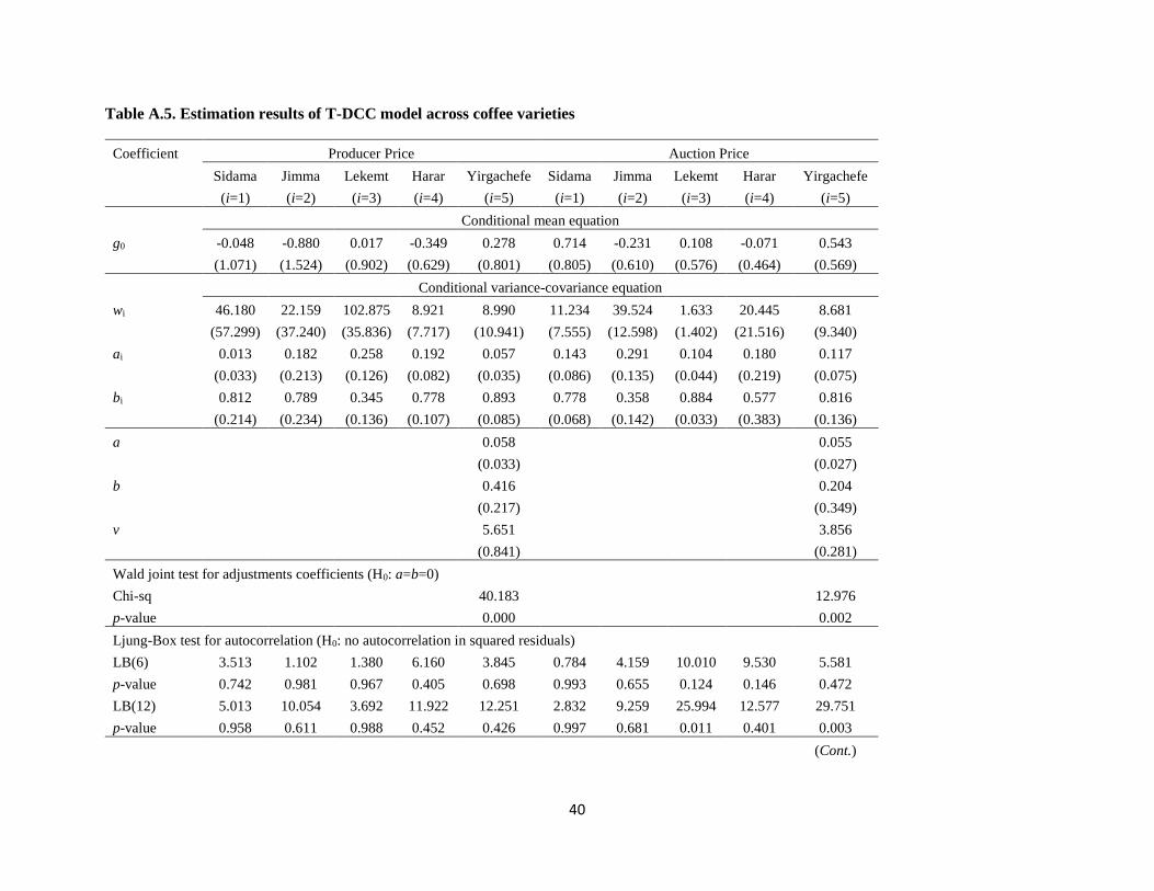
40

Table A.5. Estimation results of T-DCC model across coffee varieties

Coefficient Producer Price Auction Price

Sidama Jimma Lekemt Harar Yirgachefe Sidama Jimma Lekemt Harar Yirgachefe

(i=1) (i=2) (i=3) (i=4) (i=5) (i=1) (i=2) (i=3) (i=4) (i=5)

Conditional mean equation

g0 -0.048 -0.880 0.017 -0.349 0.278 0.714 -0.231 0.108 -0.071 0.543

(1.071) (1.524) (0.902) (0.629) (0.801) (0.805) (0.610) (0.576) (0.464) (0.569)


wi 46.180 22.159 102.875 8.921 8.990 11.234 39.524 1.633 20.445 8.681

(57.299) (37.240) (35.836) (7.717) (10.941) (7.555) (12.598) (1.402) (21.516) (9.340)

ai 0.013 0.182 0.258 0.192 0.057 0.143 0.291 0.104 0.180 0.117

(0.033) (0.213) (0.126) (0.082) (0.035) (0.086) (0.135) (0.044) (0.219) (0.075)

bi 0.812 0.789 0.345 0.778 0.893 0.778 0.358 0.884 0.577 0.816

(0.214) (0.234) (0.136) (0.107) (0.085) (0.068) (0.142) (0.033) (0.383) (0.136)

a 0.058 0.055

(0.033) (0.027)

b 0.416 0.204

(0.217) (0.349)

v 5.651 3.856

(0.841) (0.281)

Wald joint test for adjustments coefficients (H0: a=b=0)

Chi-sq 40.183 12.976

p-value 0.000 0.002


LB(6) 3.513 1.102 1.380 6.160 3.845 0.784 4.159 10.010 9.530 5.581

p-value 0.742 0.981 0.967 0.405 0.698 0.993 0.655 0.124 0.146 0.472

LB(12) 5.013 10.054 3.692 11.922 12.251 2.832 9.259 25.994 12.577 29.751

p-value 0.958 0.611 0.988 0.452 0.426 0.997 0.681 0.011 0.401 0.003

(Cont.)

41

Coefficient Producer Price Auction Price

Sidama Jimma Lekemt Harar Yirgachefe Sidama Jimma Lekemt Harar Yirgachefe

(i=1) (i=2) (i=3) (i=4) (i=5) (i=1) (i=2) (i=3) (i=4) (i=5)


LM(6) 3.060 1.073 1.360 6.932 3.319 0.781 4.395 9.026 8.901 5.052

p-value 0.801 0.983 0.968 0.327 0.768 0.993 0.623 0.172 0.179 0.537

LM(12) 4.188 9.592 3.340 12.967 12.140 1.445 8.223 19.517 13.714 27.212

p-value 0.980 0.652 0.993 0.371 0.434 1.000 0.767 0.077 0.319 0.007


M(6) 121.765 155.213

p-value 0.944 0.326

M(12) 297.777 281.790

p-value 0.493 0.742

Log likelihood -5,274.5 -4,609.3

SBIC 41.598 36.441

# obs. 258 258

Note: Standard errors reported in parentheses. ν is the degrees of freedom parameter. LB, LM and M stand for the corresponding Ljung-Box, Lagrange Multiplier

and Hosking test statistics.

42

Table A.6. Estimation results of T-BEKK model, period 1992-2008





ci1 12.497 -2.994 -3.688 3.998 -0.062 5.263 -0.002 0.002 0.002 3.405 0.569 4.766 1.625 4.359 -5.240

(3.276) (1.730) (4.252) (7.065) (0.053) (2.019) (0.034) (0.055) (0.041) (1.074) (7.120) (0.943) (1.771) (1.422) (1.801)

ci2 -0.002 -0.002 0.000 0.005 0.003 0.000 6.078 0.707 0.024 -0.026

(0.040) (0.068) (0.038) (0.021) (0.023) (0.021) (0.952) (5.772) (0.298) (0.122)

ci3 -0.001 0.005 0.000 0.000 0.002

(0.060) (0.009) (0.029) (0.058) (0.046)

ai1 0.312 0.070 0.053 0.263 -0.026 0.170 0.123 -0.103 0.037 0.652 0.017 0.099 0.650 -0.005 -0.025

(0.169) (0.096) (0.050) (0.448) (0.085) (0.096) (0.080) (0.061) (0.022) (0.130) (0.139) (0.103) (0.228) (0.126) (0.088)

ai2 -0.099 0.299 -0.190 0.350 0.268 -0.209 0.018 0.269 -0.154 0.099 -0.510 0.302 -0.041 0.926 -0.283

(0.204) (0.119) (0.088) (0.366) (0.225) (0.112) (0.048) (0.073) (0.038) (0.203) (0.325) (0.185) (0.199) (0.227) (0.188)

ai3 -1.130 0.038 -0.152 -0.109 0.111 0.190 -0.171 -0.261 0.177 -0.242 -0.261 -0.565 0.132 0.104 -0.043

(0.240) (0.160) (0.183) (0.161) (0.142) (0.102) (0.109) (0.094) (0.086) (0.188) (0.141) (0.173) (0.128) (0.111) (0.144)

gi1 -0.128 -0.480 -0.254 0.817 0.183 0.064 0.966 -0.039 -0.052 0.802 0.086 -0.038 0.601 0.060 -0.055

(0.233) (0.108) (0.149) (0.150) (0.021) (0.061) (0.019) (0.071) (0.014) (0.078) (0.103) (0.068) (0.182) (0.130) (0.060)

gi2 0.596 0.575 0.082 -0.946 0.871 0.143 -0.354 -0.725 0.315 -0.064 0.078 0.035 -0.712 0.398 0.223

(0.290) (0.134) (0.157) (0.580) (0.096) (0.183) (0.255) (0.149) (0.183) (0.428) (0.152) (0.180) (0.167) (0.198) (0.094)

gi3 0.072 -0.396 0.665 -0.545 -0.089 0.574 0.386 0.951 0.817 -0.278 -0.001 0.701 0.655 0.512 0.754

(0.956) (0.400) (0.298) (1.272) (0.142) (0.346) (0.146) (0.170) (0.141) (0.085) (0.086) (0.101) (0.249) (0.130) (0.152)

Ν 4.995 4.438 6.597 4.214 3.164

(0.983) (0.952) (1.580) (0.796) (0.524)

Wald joint test for cross-volatility coefficients (H0: aij=gij=0,i≠j)

Chi-sq 255.295 1737.751 337.627 44.105 127.233

p-value 0.000 0.000 0.000 0.000 0.000

(Cont.)

43





LB(6) 5.759 1.963 15.511 4.570 11.230 4.111 23.415 5.520 18.461 2.983 22.124 11.483 2.101 2.993 23.566

p-value 0.451 0.923 0.017 0.600 0.082 0.662 0.001 0.479 0.005 0.811 0.001 0.075 0.910 0.810 0.001

LB(12) 10.315 7.056 16.911 7.001 14.182 8.290 26.837 10.597 20.796 7.249 24.702 15.531 3.568 17.917 25.634

p-value 0.588 0.854 0.153 0.858 0.289 0.762 0.008 0.564 0.053 0.841 0.016 0.214 0.990 0.118 0.012


LM(6) 4.874 1.356 15.109 4.078 10.845 3.580 17.461 5.607 18.303 3.271 18.098 11.703 2.497 3.519 22.875

p-value 0.560 0.968 0.019 0.666 0.093 0.733 0.008 0.469 0.006 0.774 0.006 0.069 0.869 0.741 0.001

LM(12) 8.968 4.374 15.403 7.563 12.717 5.538 21.618 9.074 18.307 7.968 31.458 16.006 4.169 20.520 23.111

p-value 0.706 0.976 0.220 0.818 0.390 0.938 0.042 0.697 0.107 0.788 0.002 0.191 0.980 0.058 0.027


M(6) 58.992 67.272 77.067 60.453 59.595

p-value 0.298 0.106 0.021 0.254 0.279

M(12) 87.327 111.411 103.478 91.541 90.283

p-value 0.928 0.392 0.605 0.872 0.891

Log likelihood -2,315.9 -2,349.3 -2,288.6 -2150.5 -2243.6

SBIC 23.356 23.684 23.089 21.735 22.648

# observations 204 204 204 204 204



44

Table A.7. Estimation results of T-BEKK model, period 2009-2013





ci1 3.986 3.930 3.843 -2.891 0.985 1.519 7.614 2.518 0.745 7.599 5.934 -1.638 4.941 3.383 3.383

(5.762) (1.617) (1.100) (1.980) (1.772) (1.131) (2.845) (1.438) (1.423) (1.796) (1.428) (1.018) (4.121) (1.911) (1.470)

ci2 0.001 0.000 0.000 0.000 0.000 0.000 -0.014 -0.001 0.000 0.000

(0.188) (0.155) (0.180) (0.056) (0.128) (0.088) (0.056) (0.030) (0.156) (0.048)

ci3 0.000 0.000 0.000 0.002 0.000

(0.267) (0.095) (0.110) (0.052) (0.096)

ai1 -0.065 0.460 0.138 0.278 -0.183 -0.183 -0.812 -0.037 -0.044 -0.514 0.197 0.070 -0.083 0.216 0.213

(0.214) (0.135) (0.093) (0.272) (0.217) (0.107) (0.384) (0.201) (0.135) (0.126) (0.095) (0.045) (0.746) (0.408) (0.135)

ai2 -0.151 -0.161 0.177 0.899 0.196 0.066 -1.233 -0.062 -0.138 0.576 0.309 0.321 0.655 0.177 0.054

(0.169) (0.205) (0.158) (0.634) (0.200) (0.051) (0.519) (0.307) (0.223) (0.202) (0.126) (0.077) (0.568) (0.369) (0.131)

ai3 0.662 1.170 0.449 1.086 -0.020 -0.196 1.037 -0.466 -0.294 -0.786 0.132 0.447 0.342 -0.527 0.600

(0.453) (0.302) (0.325) (0.756) (0.346) (0.181) (0.846) (0.606) (0.261) (0.481) (0.149) (0.129) (0.526) (0.627) (0.207)

gi1 -0.464 -0.268 0.175 -0.066 0.088 0.126 -0.020 0.006 -0.372 0.553 0.189 0.092 -0.475 -0.380 0.096

(0.145) (0.172) (0.145) (0.166) (0.169) (0.179) (0.167) (0.106) (0.106) (0.163) (0.071) (0.053) (0.848) (0.683) (0.279)

gi2 1.330 0.008 0.107 0.462 -0.681 0.276 -0.254 -0.583 -0.098 -0.456 0.011 0.328 0.660 -0.291 -0.425

(0.378) (0.949) (0.507) (0.386) (0.335) (0.195) (0.814) (0.350) (0.287) (0.277) (0.016) (0.091) (0.395) (0.248) (0.214)

gi3 -1.865 0.417 0.197 0.995 1.430 0.427 -0.381 0.835 0.536 1.101 -0.903 0.197 -0.727 -0.628 0.203

(0.814) (0.853) (0.548) (0.686) (0.267) (0.719) (0.309) (0.259) (0.199) (0.302) (0.226) (0.147) (0.816) (1.120) (0.508)

ν 6.807 20.178 4.919 815.858 6.289

(4.035) (45.520) (2.239) (197.076) (2.860)

Wald joint test for cross-volatility coefficients (H0: aij=gij=0,i≠j)

Chi-sq 1023.340 361.019 658.147 365.035 343.127

p-value 0.000 0.000 0.000 0.000 0.000

(Cont.)

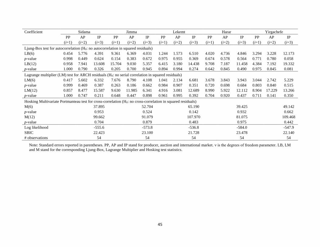
45





LB(6) 0.454 5.776 4.391 9.361 6.369 4.031 1.244 1.573 6.510 4.020 4.736 4.846 3.294 3.228 12.173

p-value 0.998 0.449 0.624 0.154 0.383 0.672 0.975 0.955 0.369 0.674 0.578 0.564 0.771 0.780 0.058

LB(12) 0.958 7.941 13.608 15.704 9.030 5.357 6.415 3.180 14.438 9.708 7.187 11.458 4.384 7.192 19.332

p-value 1.000 0.790 0.326 0.205 0.700 0.945 0.894 0.994 0.274 0.642 0.845 0.490 0.975 0.845 0.081


LM(6) 0.417 5.602 6.332 7.676 8.790 4.108 1.041 2.134 6.681 3.678 3.843 3.943 3.044 2.742 5.229

p-value 0.999 0.469 0.387 0.263 0.186 0.662 0.984 0.907 0.351 0.720 0.698 0.684 0.803 0.840 0.515

LM(12) 0.857 8.477 15.587 9.630 11.985 6.341 4.916 3.081 12.689 8.990 5.922 12.112 8.904 17.229 13.266

p-value 1.000 0.747 0.211 0.648 0.447 0.898 0.961 0.995 0.392 0.704 0.920 0.437 0.711 0.141 0.350


M(6) 37.895 52.704 65.190 39.425 49.142

p-value 0.953 0.524 0.142 0.932 0.662

M(12) 99.662 91.079 107.970 81.075 109.468

p-value 0.704 0.879 0.483 0.975 0.442

Log likelihood -555.6 -573.8 -536.8 -584.0 -547.9

SBIC 22.423 23.100 21.728 23.478 22.140

# observations 54 54 54 54 54



46

Table A.8. Estimated break dates for price returns and squared price returns

Market Returns Squared returns

Sidama

Producer price Dec 2010 Dec 2010

Auction price May 1994 Feb 1999

Jimma

Producer price May 2002 Jul 2003

Auction price Jun 1994 Sep 1994

Lekemt

Producer price Dec 2010 Oct 2000

Auction price Aug 1995 Sep 1994

Harar

Producer price Apr 2011 Dec 2002

Auction price Apr 1994 May 1994

Yirgachefe

Producer price Feb 2012 Jan 1998

Auction price Aug 1997 Sep 1997

International price Apr 1994 Apr 1994

Note: The estimated break dates are based on Lavielle and Moulines (2000) test for structural breaks on the mean of

price returns and the squared of price returns as a proxy of volatility. Minimum length of a segment is 2 months.

47

Figure A.1. Growing areas of Arabica coffee in Ethiopia, 2009-2013

Note: Map based on weighted production average period 2009-2013. Volume of production obtained from Central

Statistical Agency (CSA). Sid=Sidama; Jim=Jimma; Lek=Lekemt; Har=Harar; Yir=Yirgachefe; SNNPR= Southern

Nations Nationality Peoples region.

48

Figure A.2. Average conditional correlations for different subperiods based on T-DCC model across coffee varieties

Producer level

Auction level

Note: The conditional correlations are derived from the estimation results of the T-DCC model. The vertical lines are confident bands of one standard deviation.

-0.2

-0.1

0.0

0.1

0.2

0.3

0.4

0.5

0.6

Sidama-Jimma Sidama-Lekemt Sidama-Harar Sidama-Yirgachefe Jimma-Lekemt

Jan 1992-Dec 1995 Jan 1996-Dec 2004 Jan 2005-Dec 2008 Jan 2009-Jun 2013

-0.2

-0.1

0.0

0.1

0.2

0.3

0.4

0.5

0.6

Jimma-Harar Jimma-Yirgachefe Lekemt-Harar Lekemt-Yirgachefe Harar-Yirgachefe


-0.1

0.0

0.1

0.2

0.3

0.4

0.5

0.6

Sidama-Jimma Sidama-Lekemt Sidama-Harar Sidama-Yirgachefe Jimma-Lekemt


-0.1

0.0

0.1

0.2

0.3

0.4

0.5

0.6

Jimma-Harar Jimma-Yirgachefe Lekemt-Harar Lekemt-Yirgachefe Harar-Yirgachefe


The Ethiopian Commodity Exchange and the coffee … Ethiopian Commodity Exchange and the coffee...

Documents

Transcript of The Ethiopian Commodity Exchange and the coffee … Ethiopian Commodity Exchange and the coffee...