The Ending of the Trade Policy Bias Against Agriculture:

Evidence for Indonesia and Thailand*

Peter Warr

The Australian National University

December 2007

1. Introduction and summary

In a famous multi-country study for the World Bank, Krueger, Schiff, and Valdés (1988) documented

a consistent and widespread trade policy bias in developing countries. The bias operated against

agriculture and in favour of manufacturing and this pattern was demonstrated throughout Africa,

Latin America and Asia, including most countries of Southeast Asia. The data used in that study

covered the period ending in the late 1970s. The present paper asks whether that pattern can still be

detected today, using updated information for two Southeast Asian countries – Indonesia, a major

food importer, and Thailand, a major exporter.

The analysis is based on detailed comparisons between the prices of agricultural commodities

in domestic and international markets. The analysis confirms the Krueger et al. conclusion for the

period covered by their study but concludes that since then the overall structure of protection has

shifted markedly. Overall, protection is now roughly neutral between agriculture and manufacturing

in both countries. Nevertheless, despite this change in the overall bias of trade policy there remains

considerable variation in the protection accorded to different agricultural industries.

The discussion in the present paper focuses on just three important commodities: rice, sugar

and an important input, urea fertilizer. Detailed analyses on a wider range of agricultural commodities

is available in Fane and Warr (2007) and Warr and Kohpaiboon (2007), both available online, and

these analyses support the conclusions of this paper.

2. Indonesia

In Indonesia, the staple food, rice, is a net import and this one commodity has been a central focus of

Indonesian food policy throughout the (almost) six decades since the country’s Independence. Self-

sufficiency in rice, meaning the elimination of rice imports, has been a cherished goal of agricultural

policy for all of this time. It is an emotive subject, closely linked in the public imagination to

Indonesian nationalism. When asked his proudest single achievement, Soeharto, Indonesia’s president

* This paper draws on earlier work with George Fane (Indonesia) and Archanun Kohpaiboon (Thailand), undertaken for the World Bank. The excellent research assistance of Arief Ramayandi is gratefully acknowledged. The author accepts responsibililty for all defects.

2

for the 32 years from 1966 to 1998, cited the (temporary) achievement of self-sufficiency in rice. This

paper documents the changing structure of agricultural protection in Indonesia and attempts to explain

the forces that have driven it.

2.1 Policy evolution

Indonesia obtained its independence from the Netherlands in 1949. The next two decades were

chaotic. The post-Independence government of President Soekarno pursued a nationalistic, quasi-

socialist economic policy that produced hyperinflation and economic stagnation. In 1966 Soekarno

was displaced amid economic chaos by one of his generals, Soeharto, whose regime, called the ‘New

Order’, lasted until the macroeconomic crisis of 1998. Soeharto pursued more market-oriented

economic policies than his predecessor. Upon assuming power, Soeharto speedily introduced a

macroeconomic stabilization program and then began liberalizing Indonesia’s trade and investment

policies. In 1967 foreign investors were guaranteed the right to repatriate both capital and profit and

from 1970 onwards the capital account was almost completely open. As we shall see below, trade

policy under Soeharto’s government was much less open. It was characterized by taxation of exports,

especially non-food agricultural exports, and protection of imports, including some food imports.

In the wake of the commodity boom of 1972-73 and the oil price shocks of 1973-74 and

1979-80, trade policy became increasingly inward-looking. As Figure 3 shows, these external events

tripled the ratio of Indonesia’s export prices to its import prices. Between the early 1970s and the mid-

1980s the government taxed or banned some traditional exports, pursued self-sufficiency in rice, and

used part of the burgeoning oil revenues to establish import-substituting manufacturing industries,

which it then protected. In the early to mid-1980s several traditional export industries were subjected

to quantitative trade restrictions. These included a ban on log exports, conferring very high rates of

effective protection on the plywood manufacturing industry, for which raw timber is the principal

input. Licensing systems were introduced for exports of vegetable oils, several spices, coffee and

some grades of rubber. In the case of palm oil, domestic refiners were protected by a tax on exports

and a requirement that growers supply these refiners with part of their output at low, controlled prices.

From 1982 onwards, the price of oil began to decline. By the mid 1980s it had fallen from

US$28 to $10 per barrel. Many oil-exporting countries, including Nigeria and Venezuela, were unable

to adjust to these external changes without devastating domestic consequences, but Indonesia

responded quickly by cutting public spending and devaluing its currency, partly to promote non-oil

exports. In addition, a value added tax (VAT) was introduced between 1983 and 1986. At first, trade

policy became increasingly oriented towards import substitution and the system of import licensing

was extended. But after this initial protectionist response to lower petroleum export revenues, trade

policy was significantly liberalized from 1985 onwards.

3

With the stated goal of promoting non-oil exports, the government introduced a series of

reforms which reduced tariffs and non-tariff barriers (NTBs). Following tariff cuts in 1985 the

government transferred most customs functions from the Indonesian Customs Service to an

international inspection company, SGS of Switzerland. The role of SGS was phased out by 1995.

NTBs on imports were progressively relaxed from 1986 onwards and the system of providing

exporters with duty-free inputs was extended.

According to the estimates of Fane and Condon (1996), the effective rate of protection in

agriculture declined from 24 percent in 1987 to 14 percent in 1994, and that in manufacturing

declined much further, from 86 percent to 29 percent over the same period. Since there was probably

more ‘water’ in the tariffs in 1987 than in 1995, the true reductions in protection were probably

somewhat smaller than these numbers indicate, but the decline was still substantial. In addition to the

lowering of tariff rates, many NTBs were replaced by tariffs. The coverage of ‘restrictive’ NTBs

declined from 44 percent of total value added in all traded industries in 1986 to 23 percent in 1995.

This switch from NTBs to tariffs was somewhat more extensive in manufacturing than in agriculture,

where the coverage of NTBs declined from 67 to 48 percent. In the wake of the financial crisis of

1997–98, the government was obliged to allow free imports of both rice and sugar as a condition for

borrowing from the IMF. However, with the ending of the IMF program, imports of rice and sugar

have again been restricted by both tariffs and NTBs.

2.2 Agricultural protection by sector

Rice

The most important and most enduring non-tariff barriers have been those on rice and sugar. Figure 3

shows estimates of domestic wholesale prices and border prices for rice.1 All the price series in these

charts are in rupiah per kilogram, divided by the GDP deflator, indexed at 2005 = 1. While there have

been enormous nominal increases in rice and sugar prices since the early 1970s, the charts show that

any trends in the real prices of these products have been relatively small.

It is clear from Figure 1 that the domestic wholesale price of rice has fluctuated much less

than the border price and that domestic prices have not differed greatly, on average, from the trend

level of border prices. Price stabilization was achieved by giving the state logistics agency, Bulog

(Badan Urusan Logistik), a monopoly over international trade in rice and directing it to build up buffer

stocks to smooth out fluctuations in domestic supply. It is significant that this stabilization of

1 The border price of rice in Figure 4 has been converted to make it as nearly comparable as possible to the wholesale price. The fob price was adjusted to the cif level by adding freight and insurance costs; the resulting cif price was then adjusted to the wholesale level by adding margins to allow for the estimated handling, warehousing and interest costs.

4

domestic prices was achieved while keeping the trend value of domestic prices roughly in line with

the trend of world prices. Average rates of protection in the output market for rice were very low.

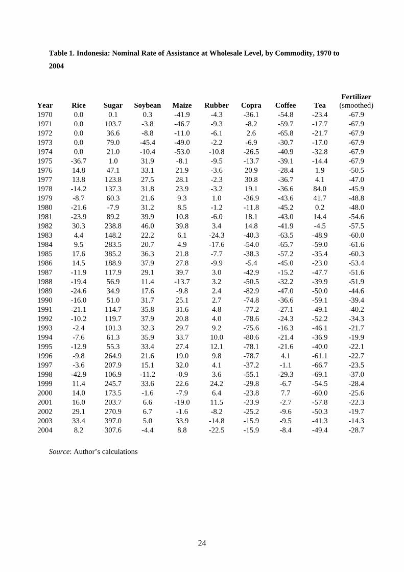
This low rate of protection for rice is shown in Table 1, which summarizes nominal rates of

protection for 8 major agricultural commodities (including rice) plus urea fertilizer. These estimates

are based on comparisons of the annual average domestic wholesale prices of these commodities with

their corresponding c,i.f. import prices or their f.o.b. export prices, whichever is relevant, the latter

adjusted by estimates of the transport and handling costs incurred between the border and the

wholesale level. The resulting annual estimates vary from year to year, partly because of fluctuations

in international prices and because changes in these border prices are seldom transmitted immediately

to domestic markets. Our interest is in broad changes over time, rather than year to year fluctuations.

In the late 1980s, the strict policy of zero imports of rice was replaced by a policy of

‘borrowing’ rice from Vietnam in times of shortage and repaying the rice loans in times of surplus.

These ‘loans’ were conducted in bilateral government-to-government deals in which Bulog acted for

the Indonesian government. In the early 1990s, it gradually became apparent that Indonesia was

unable to maintain rice self-sufficiency, even on average and over a period of years. To satisfy

domestic demand at ‘acceptable’ prices, Bulog was forced to undertake substantial net imports.

When the Asian crisis forced Indonesia to borrow from the IMF in 1997, one of the loan

conditions to which the government agreed was the removal of Bulog’s monopoly on rice imports.

Until 1999, there was also no import duty on rice but the IMF’s aim of free trade in rice proved

illusory because the financial crisis briefly converted rice into a potential export and the government

banned exports to reduce pressure on domestic prices. Figure 4 shows that in 1998 border prices,

converted to rupiah at the devalued exchange rate, were far above domestic prices. The reason for this

was that the massive depreciation of the exchange rate between mid-1997 and mid-1998 initially

outweighed the much more gradual rise in domestic prices. This episode clearly demonstrated that the

government’s policy has always been to stabilize food prices at ‘acceptable’ levels, rather than simply

to protect growers.

The general increase in domestic prices in 1998-99 and the stabilization of the exchange rate

after mid-1998 removed the incentive to export rice. Bulog’s monopoly on imports was not

immediately re-imposed, but a 20 percent tariff on rice imports was introduced in 1999. Problems

with under-invoicing by importers resulted in this tariff being converted to a specific tariff at Rp

430/kg. In 2002, Bulog’s monopoly over imports was restored and since 2004 imports have officially

been banned, although Bulog has occasionally been issued with special import permits.

Sugar

The Indonesian sugar industry is dominated by the state-owned mills, mainly on Java, that were

acquired by the nationalization of the formerly Dutch-owned sugar estates in 1957. Investment and

technical progress in this sector has been extremely sluggish and the industry has languished behind

5

protective barriers. The finished product of these antiquated factories, known as ‘plantation white

sugar’, is not exactly comparable to either the refined or the raw sugar traded on the world market.

Plantation white contains more impurities—mainly molasses—than internationally traded raw sugar,

but has already undergone some of the bleaching processes that separate refined from raw sugar in

more technologically advanced sugar industries. Most firms in the food and beverage sectors cannot

use plantation white sugar because of its relatively high level of impurities; their needs are mainly met

by imports of raw sugar, although there is a small amount of raw sugar produced domestically.

As in the case of rice, the main motive behind government policy for sugar appears to be the

desire to stabilize the domestic price at an ‘acceptable’ level. In addition, in the case of sugar, the

government has tried to protect the sugar factories that it owns. This may explain why, at least since

1957, the sugar industry has been more tightly regulated than any other agricultural sector, with the

government monopolising not only imports but also domestic marketing. Government ownership also

helps to explain newspaper reports that, in the 1970s, farmers in traditional sugar growing areas were

regularly forced to grow sugar to supply local factories, subject to threats that other crops would be

burnt.

Figure 2 compares the border price of raw sugar (after allowing for margins between fob

price and domestic wholesale prices) with the domestic wholesale price of plantation white sugar. The

chart shows that for much of the period since 1970, domestic prices were about twice the border price,

implying a nominal rate of protection (NRP) of about 100 percent. However, in 2006 this gap has

been have been greatly narrowed by the abrupt rise of world prices.

Our estimates of the NRP for sugar ignore two factors, the first of which makes our estimates

tend to understate the true NRP, while the second goes in the opposite direction. The first factor is

that our estimates make no adjustment for the relatively low polarity (high level of impurities) of

plantation white sugar. The offsetting factor is the neglect of the cost of bleaching to obtain plantation

white sugar. Experts on the sugar industry have suggested that the low polarity effect is probably

more important than the effects of bleaching, but that the difference is small.

Fertilizer

Input markets were another matter. From the 1970s onwards, the Soeharto government used part of its

new oil wealth to promote self-sufficiency in rice, by subsidising the adoption of high yielding

varieties that had been made available by the ‘Green Revolution’. These new varieties required

greatly increased use of irrigation, fertilisers and pesticides, which the government helped to finance.

An important motivation for this policy was fear of a repetition of the riots precipitated by high food

prices in 1965.

Under the Bimas program, introduced with the explicit goal of rice self-sufficiency, farmers

received agricultural extension services and subsidized credit, seeds, fertilisers and pesticides. The

6

government also paid for increasing and upgrading irrigation facilities. The resulting increase in the

profitability of rice growing, together with some coercion of those farmers who were reluctant to

extend the area of rice cultivated, led to a 17 percent increase in gross2 harvested area in the decade to

1985. This increase in area, together with a 50 percent increase in average yields in the same period,

allowed Bulog to reduce domestic rice prices relative to the CPI between the late 1970s and 1985

while gradually phasing out imports and then halting imports altogether in 1985.

Lower world oil prices and advice from the World Bank contributed to the reduction in

agricultural input subsidies in the late 1980s and early 1990s. Figure 3 shows a fall in the real price of

urea from the late 1970s to the early 1980s and a subsequent rise in the domestic wholesale price of

urea relative both to the CPI and to the border price in the late 1980s and early 1990s. Exports of urea

require special approval from the Ministry of Trade, under an export licencing scheme. The year to

year determination of the magnitude of these licences is non-transparent, but the Ministry tends to

place priority on ensuring that domestic supplies are stable at a price lower than world market prices

and this results in the negative nominal rates of protection shown in Figure 3.

2.3 Imputed protection at the farm level

So far, the discussion of protection has related to the effects that policy interventions have at the

wholesale market level. In this section, the analysis is extended to consider the way protection (or its

opposite) at the wholesale level produces price effects at the farm level.

Theory

One of the intentions of agricultural protection policy is to influence prices at the farm level. But the

goods produced directly by farmers seldom enter international trade themselves. The raw

commodities produced by farmers are generally non-traded, whereas the commodities which enter

international trade are the processed or partially processed versions of these raw products. Between

the non-traded raw product produced by the farmer and the traded processed commodity which enters

international trade, there may be several steps of transport, storage, milling, processing and re-

packaging.

The significance of this point is that protection policy operates directly on the goods which

actually enter international trade, either exported or imported, not the raw commodities produced by

farmers. Protection at the farm level is therefore a derived effect. It depends on the extent to which

policies applied to trade in processed agricultural goods induce changes in their prices which are then

transmitted to the prices actually faced by farmers. The question thus arises as to what extent price

changes at the wholesale level, induced by protection policy, affect the prices actually received by

2 "Gross" indicates that a hectare which is harvested twice in a year is counted as 2 hectares.

7

farmers for the raw products they sell.

We construct a simple econometric model to investigate this issue. We shall use the

notational convention that upper case Roman letters (like X ) will denote the values of variables in

their levels and lower case Roman letters (like x ) will denote their natural logarithms. Thus

Xx ln= . Protection at the wholesale level is defined as

)1(* Witit

Wit TPP += , (1)

where WitP denotes the level of the wholesale price of commodity i at time t, *

itP is the corresponding

border price, expressed in the domestic currency and adjusted for handling costs in getting the

commodity from the cif level to the domestic wholesale level, in the case of an import, and for the

cost of getting it from the wholesale level to the fob level in the case of an export. The nominal rate of

protection at the wholesale level is given by WitT . In this discussion, both the border price and the

nominal rate of protection are treated as exogenous variables. The border price is determined by world

markets and the country concerned is presumed to be a price taker. The nominal rate of protection is

determined by the government’s protection policy.

The farm gate price of the raw material is denoted by FitP and its logarithm, F

itp , is related to

the logarithm of the wholesale price by

itWitii

Fit upbap ++= , (2)

where ia and ib are coefficients and itu is a random error term. The coefficient ib is the ‘pass-

through’ or ‘transmission’ elasticity. The estimated values of the coefficients ia and ib are denoted

ia and ib , respectively. The econometric estimation of these parameters is discussed below.

The estimated coefficients are used as follows. We estimate the logarithm of the farm price

that would obtain in the absence of any protection as

** ˆˆˆ Witii

Fit pbap += , (3)

where *Witp is the estimated value of the wholesale price that would obtain in the absence of

protection, ** ln Wit

Wit Pp = . This is then compared with the estimated value of the wholesale price in

the presence of protection

8

Witii

Fit pbap ˆˆˆ += . (4)

Denoting the anti-logs of Fitp and *ˆ F

itp by FitP and *ˆ F

itP , respectively. The nominal rate of protection

at the farm level is then estimated as

F

itF

itF

itF

it PPPT ˆ/)ˆˆ(ˆ *−= . (5)

It is important to observe that the value of the protection-inclusive farm level price used in

these calculations is the level estimated from the econometric model (equation (4)) rather than the

actual price given by the raw data. The reason is that our intention is to use the model to estimate the

change in the farm gate price caused by protection at the wholesale level. Thus both the protection-

inclusive and the protection-exclusive prices used in (5) are their predicted values, obtained from the

model.

The implied nominal rate of protection at the farm level can be related to the nominal rate of

protection at the wholesale level, as follows. Substituting ibWiti

Fit PAP ˆ)(ˆˆ = and ibW

itiF

it PAP ˆ** )(ˆˆ = into

equation (5), where iA is the anti-log of ia , rearranging, and using equation (1), we obtain the simple

expression

1)1(ˆ ˆ−+= ibW

itF

it TT . (6)

Obviously, if 0=WitT , then 0ˆ =F

itT , regardless of the value of ib . Similarly, if 0ˆ =ib , then

0ˆ =FitT , regardless of the value of W

itT . Also, if 1ˆ =ib , then Wit

Fit TT =ˆ . It can readily be seen that

when 0>WitT , W

itF TT ≥ˆ as 1ˆ ≥ib and W

itF TT ≤ˆ as 1ˆ ≤ib . When 0<W

itT , Wit

F TT ≤ˆ as 1ˆ ≥ib

and Wit

F TT ≥ˆ as 1ˆ ≤ib .

Econometric application

The purpose of the econometric analysis is to estimate the parameter ib for each commodity. Details

of the econometric analysis are provided in a statistical appendix, available upon request. Here the

results will be summarized. For each commodity we conduct the analysis using time series price data

with each variable expressed in logarithms and each deflated by the GDP deflator for Indonesia: the

farm gate price (LFP), the wholesale price (LWP), and the log of the international price, adjusted by

the nominal exchange rate and transport and handling costs (LIP). The data extended from 1976 to

9

2001. The seven commodities for which these data were available were: rice, maize, soybeans, sugar,

rubber, coffee and tea.

We first test each of the series (each deflated by the GDP deflator) for the existence of a unit

root. For rice, the null hypothesis of a unit root was rejected for all three price series (recalling that

they are real, not nominal, price series, using the GDP deflator) at the 10 per cent level of

significance. The price series were thus considered stationary. For other commodities the results were

more mixed. For maize, the null hypothesis of a unit root could not be rejected for farm level prices

(LFP), but was strongly rejected for the other two price series. For soybeans, the null hypothesis of a

unit root could not be rejected for the wholesale price series (LWP) but was rejected at the 10 per cent

level for the other two series. For sugar, the null hypothesis of a unit root could not be rejected for any

of the three series, expecially the farm level price series (LFP). For rubber, coffee and tea the results

were similar. The null hypothesis of a unit root marginally failed to be rejected for the farm level

price series (LFP), but was rejected for the other two series.

Ordinary least squares (OLS) estimates of equation (2) were first produced. In most cases,

autocorrelation was a problem and an AR(1) correction term was included to eliminate it, which it did

effectively. The OLS estimates assume that LFP is endogenous and LWP is exogenous. These

assumptions were tested using Hausman’s endogeneity test, although it is recognized that the test has

low power when the number of data points is small, as in this case. In the case of each commodity, the

null hypothesis that LWP was (weakly) exogenous to LFP failed to be rejected, confirming the

validity of the OLS estimates. Reverse Hausman’s tests were also conducted and the null hypothesis

that LFP was exogenous to LWP was rejected in the cases of maize, sugar, rubber, coffee and tea. It

marginally failed to be rejected for rice and soybeans. These results roughly support the validity of

using the OLS framework to estimate the transmission elasticity from LWP to LFP, treating LWP as

exogenous.

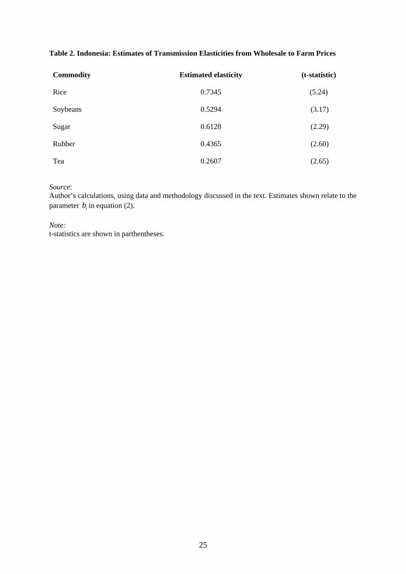
Usable estimates were produced for five commodities: rice, soybeans, sugar, rubber and tea.

For each of these commodities, the estimated elasticity had the expected positive sign and was

significantly different from zero, with the estimated equation performing well. Table 2 summarizes

the estimates. For maize and coffee, the estimated elasticity was not significantly different from zero

and the estimated equation performed poorly. It is often asserted that middlemen prevent commodity

price changes at the wholesale level, resulting from protection or from international price movements,

from being transmitted to farmers. This hypothesis is rejected by the Indonesian data, at least for the

five commodities mentioned above. The transmission elasticities are not zero. Economists typically

assume that the transmission elasticities are unity. But the Indonesian data reject that hypothesis as

well. The estimated values are generally less than unity, lying between 0.2 and 0.8. The lower values

are obtained in the case of perennial crops rubber and tea, which have high processing costs. The

other values all exceed 0.5. It is likely that the true transmission elasticities change over time, but the

limited data available for this exercise made it necessary to assume that the true values are constant.

10

Estimation of protection at farm level

Given the estimated value of the transmission elastity, equation (6) was used together with the

estimated nominal rates of protection at the wholesale level, discussed above, to produce estimates of

imputed NRPs at the farm level. These are shown in Table 3, which may be compared with the

corresponding estimates at the wholesale level summarized in Table 1, above. Because usable

estimates of the transmission elasticity could not be obtained for three commodities – maize, coffee

and copra – the estimated values for rice, tea and rubber, respectively, were used instead, as proxies

for the true elasticities for these commodities. Because the transmission elasticities lie between zero

and unity, the imputed nominal rates of protection at the farm level are somewhat lower in absolute

value than the nominal rates at the wholesale level, but (because of the assumption of constant

transmission elasticities) they track the pattern of the wholesale level results closely.

2.4 Aggregate measures of agricultural protection

In this section aggregate measures of rates of protection are calculated using the information

assembled from the preceding analysis and Warr and Fane (2007) following, as much as possible, the

methodology outlined in Anderson et al. (2006). The annual calculations reported in this section

fluctuate somewhat from year to year. International and domestic price changes from year to year

alter the protective effects of all instruments of protection except ad valorem tariffs. In addition, the

time taken for domestic prices to adjust to international price changes means that annual data on price

differences indicates some variation from one year to the next. Our interest is on broad trends, rather

than these annual fluctuations.

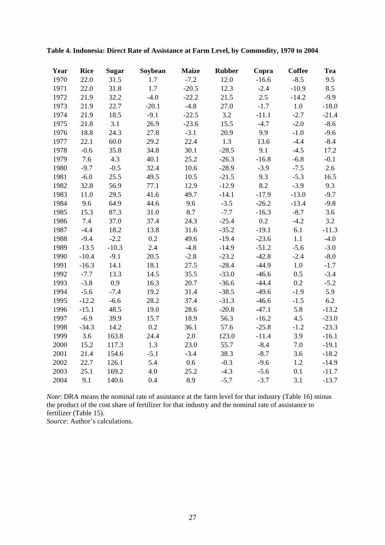
First, Table 4 calculates the direct rates of assistance at the farm level, taking account of

assistance to fertilizer inputs. The direct rate of assistance to a particular commodity is calculated as

its nominal rate of protection (synonymous with nominal rate of assistance) minus the product of the

cost share of fertilizer in production of the commodity concerned and the nominal rate of assistance to

fertilizer. The calculations use the estimates of nominal rates of protection (nominal rates of

assistance) for commodities at the farm level from Table 3 and the estimated nominal rate of

protection for fertilizer at the wholesale level from Table 1. The nominal rate of assistance to fertilizer

is negative in each year, meaning that fertilizer use is subsidized, although the rates of subsidy have

declined over time. The direct rates of assistance therefore exceed the nominal rates for every

commodity which uses fertilizer as an input.

The calculations of direct rates of assistance confirm that during the period 2000 to 2004,

import-competing commodities rice and sugar were significantly protected, especially sugar. The

rates of protection for these two commodities increased significantly compared with say a decade

earlier. Other import-competing commodities, soybeans and maize, receive little or no assistance.

11

Export commodities such as rubber, copra and coffee are either lightly taxed or untaxed today, having

been significantly taxed two decades ago. Tea exports are still moderately taxed. For the subsequent

discussion, it is notable that rates of export taxation, especially for copra, were highest in the late

1980s to mid-1990s.

Estimates of sector-wide and economy-wide rates of assistance are summarized in Table 5.

Column (5) estimates the anti-trade bias among agricultural sectors as

ATBA = (1+ DRAMA ) /(1+ DRAX

A ), (7)

where DRAMA denotes the direct rate of assistance to imported agricultural products and DRAX

A

denotes the direct rate of assistance to exported agricultural products. An ATB greater than unity

indicates that within agriculture import-competing products are more highly protected than exports. In

Indonesia, the ATB within agriculture exceeds unity most years shown and is seemingly increasing,

but it has not yet reached the levels of the first half of the 1990s.

Finally, the total rate of assistance to agriculture (column (6)) is calculated as the difference

between the direct rate of assistance to total agriculture (column (1)) and the direct rate of assistance

to manufacturing. The latter is estimated from effective rates of protection for manufacturing

estimated by Fane and Condon (1996). These authors estimate the effective rate of protection for

manufacturing, including oil and gas for 1987 and 1995 at 48 and 20 percent, respectively. They also

project the corresponding effective rate for 2003, at 13 percent, based on the May 1995 tariff

reduction package, which was to be implemented by 2003, and which was in fact largely

implemented. For all years before 1987 we have used the 1987 values, even though some tariff

reduction had occurred during the few years before 1987. For the years between 1987 and 1995 and

between 1995 and 2003, we have interpolated linearly. For 2004 we have used the 2003 value. As

noted above, the objective of this discussion is to identify broad trends over time in the structure of

protection, and not year to year changes.

These estimates show that agriculture has moved from being a net taxed sector to a net

subsidized sector. This transition occurred shortly after the Asian crisis of 1997-99. The

approximations described above undoubtedly understate rates of manufacturing protection prior to

1987. Although our estimates show negative values of the TRA for agriculture during this pre-1987

period, better estimates of manufacturing protection during this period would show larger negative

numbers. Our rough estimates for manufacturing protection therefore introduce errors whose

correction would reinforce, rather than undermine our broad conclusions.

12

3. Thailand

Thailand is a major net agricultural exporter and its agricultural trade policy is dominated by this fact.

The list of agricultural exports includes many of the most important agricultural products produced

and consumed within the country, including the staple food, rice, exports of which account for

between 30 and 50 per cent of its total output, but also cassava, sugar, rubber and poultry products.

The list of imported agricultural commodities is much thinner. Maize has been a net export in most

years but was a net import for some years in the 1990s. Soybeans was a net export for several

decades, but since the early 1990s it has become a net import. Palm oil has fluctuated between a net

import and a net export but has been a net export since the late 1990s.

3.1 Policy evolution

Historically, Thailand’s large agricultural surplus has led to a degree of policy complacency regarding

the agricultural sector. Agricultural importing countries are typically concerned about food security

and raising agricultural productivity to reduce import dependence. In Thailand, these matters have not

been a significant concern, although stabilizing food prices for consumers has been a recurrent theme

of agricultural pricing policy. Until the 1980s, agricultural exports were viewed as a source of revenue

for the central government. Unlike manufacturing, traditional agriculture was not seen as a dynamic

sector of the economy which could contribute to rapid growth. Because the price elasticity of supply

of most agricultural products was very low, at least in the short run, their production could be taxed

heavily without producing a significant contraction of output. Moreover, most agricultural producers

were impoverished, poorly educated and politically unorganized. Each of these statements applied in

particular to rice, so taxing agriculture, and especially rice, was politically attractive and rice exports

were indeed taxed until 1986.

With greatly increased incomes per person, rapid urbanization and the move to more

democratic political institutions, policy has shifted away from taxing agriculture and towards a more

neutral set of trade policies. This change has almost certainly owed more to politics – the political

necessity of finding ways to attract the support of the huge rural electorate and the desire of the urban

electorate for better economic conditions for the farm population – than to a desire to liberalize

agricultural trade for the efficiency-based reasons that economists emphasize. But the move away

from taxing agriculture has not progressed far in the direction of subsidizing it, for one key reason.

The fact that so many of the important agricultural commodities are net exports has made subsidizing

agriculture problematic, inhibiting what would otherwise have been strong political pressure to

protect Thai farmers had the commodities they produced been net imports.

Thailand is an active member of the Cairns Group of agricultural exporting countries, but while its

13

agricultural trade is relatively liberal, it cannot be described as a free-trading country with regard to

agricultural commodities. Within Thailand, opposition to agricultural import liberalization is strong in the

cases of soybeans, palm oil, rubber, rice and sugar. The measures employed include non-tariff

instruments permitting a high degree of discretion on the part of government officials. The set of import

controls includes import prohibitions, strict licensing arrangements, local content rules and requirements

for special case-by-case approval of imports. The commodities for which these restrictions are applied

include the five mentioned above and also onions, garlic, potatoes, pepper, tea, raw silk, maize, coconut

products and coffee.

The inclusion of rice in this list of commodities subject to import restrictions may seem strange.

Thailand is the world’s largest exporter of rice and is undoubtedly one of the world’s most efficient

producers. Why should its rice industry require protection from imports? Imports of rice are in fact

prohibited unless specifically approved by the Ministry of Commerce. The Ministry of Agriculture

and Cooperatives vigorously opposes any liberalization commitments with regard to rice. The reasons

apparently relate to the Ministry’s wish to keep its options open with respect to rice policy in the

event that market conditions should change unexpectedly. Sudden changes in the price of rice can

have far-reaching political consequences. The domestic rice market operates almost entirely without

government intervention, but the instruments for potential intervention are ever ready.

A lesser reason for the import controls on rice is that, as with most agricultural commodities,

‘rice’ is in fact a highly differentiated commodity. Not all grades of rice are produced efficiently

within Thailand and the government wishes to protect domestic producers from imports of grades of

rice that are closer substitutes for local grades on the consumption side than they are on the

production side. Lower grades of rice produced in Vietnam but not in Thailand are an important

example.

Thailand’s “general exclusion list”, which applies to the ASEAN Free Trade Area (AFTA)

agreements, includes several agricultural industries, including rice, sugar, palm oil (both crude and

refined). Within Thai government circles, discussion of the problems of agricultural trade relates

overwhelmingly to the treatment of Thai exports by others. Thailand’s own agricultural import policy

is a closed issue. Problems have been encountered with a number of trading partners with respect to

environmental and sanitary and phytosanitary (SPS) issues concerning Thailand’s agricultural

exports. These problems have included the well-known dispute with the United States regarding

shrimp (environmental issues) and with Australia regarding Thailand’s exports of frozen, cooked

chicken (SPS issues).

Within Thailand, poverty is heavily concentrated in rural areas and public opinion favors

government support for the rural poor. Since the economic crisis of 1997-98, and especially during

the government of Prime Minister Thaksin Shinawatra (2001-2006), a wide range of income support

programs, cash grants to villages and subsidized credit schemes was introduced. Support for these

schemes was a significant component of the ‘populist’ economic policy agenda of the Thaksin

14

government. However, few if any of these schemes operated through the prices faced by agricultural

producers. Since they were not linked directly to the production of agricultural commodities, it seems

that they were not ‘distorting’ in terms of resource allocation. The results of the present study will

make it possible to check this point. It will be possible to assess whether the price incentives facing

agricultural producers were indeed ‘distorted’ relative to international prices during this period of

populist government.

3.2 The changing structure of protection at the wholesale level

In their definitive study of agricultural price policy in Thailand up to the mid-1980s, Siamwalla and

Setboonsarng (1989 and 1991) make the point that policies for the various agricultural commodities

were determined individually, in response to political circumstances which varied among the

commodities concerned, rather than as a part of a single, integrated agricultural policy strategy. For

this reason, they argue that it is best to consider the main commodities one at a time, which they do

for the commodities rice, sugar, maize and rubber. The discussion which follows will also adopt this

strategy, except that the range of agricultural commodities considered includes cassava, soybeans and

palm oil, in addition to the four reviewed by Siamwalla and Setboonsarng, and our analysis also

considers a major input, urea fertilizer. Following this commodity-specific review, we turn to the

issue of what common themes, if any, can be found for Thai agricultural policy as a whole.

The structure of the discussion for each commodity is first to relate domestic and border

prices on a comparable basis. This analysis is conducted at the wholesale level, meaning that the

‘domestic price’ means the domestic wholesale price. All of the price data used in this analysis are

presented in the Appendix tables to Warr and Kohpaiboon (2007). We then use these data to calculate

nominal rates of protection (NRPs) for each commodity. Table 2 summarizes the price data used in

these NRP calculations and the formula used. In the calculation of the nominal rates of protection, the

border prices are amended by the transport and handling costs involved in getting imports from the cif

level to the domestic wholesale level and in getting exports from the domestic wholesale level to the

fob level. These transport and handling costs are summarized in Appendix to Warr and Kohpaiboon

(2007). This adjustment is required to obtain prices comparable with domestic wholesale prices. The

border prices adjusted by transport and handling costs are then interpreted as indications of what the

domestic wholesale prices would be in the absence of protection. The resulting estimates of nominal

rates of protection at the wholesale level for six major commodities and fertilizer are presented in

Table 6. The following discussion summarizes these results for rice, sugar and fertilizer.

Rice

From the end of World War II to 1986, Thailand taxed its exports of rice. There were four individual

instruments of export taxation, each with different legal foundations, each under the control of

15

different parts of the bureaucracy, and each generating revenues that went to different destinations

within the government. Siamwalla and Setboonsarng describe these differences but point out that their

combined effect was a rate of export taxation of around 40 per cent from the late 1950s to the early

1970s. The rate increased to around 60 per cent during the commodity price boom of 1972-74, but

subsequently diminished quickly to about 20 per cent. There was a further peak of about 40 per cent,

at the time of the second OPEC oil price shock in 1979-80, and then a steady decline until all four

forms of tax were suspended in 1986. Rice exports have remained untaxed for the two decades since

then.3

The implications of these events for actual prices are summarized in Figure 3. As with each

similar figure to be presented below for other agricultural commodities, the figure compares domestic

wholesale prices with border prices for commodities of comparable quality. Since rice is a net export,

‘border price’ in the diagram means the export price, adjusted for transport and handling costs

between the wholesale and export level. The NRP calculations that emerge are similar to those that

would be inferred from the rates of taxation described above, except that the NRPs after 1986 are not

zero, but have declined from around -11 per cent in the late 1980s to around -3 percent two decades

later, in 2005. It is possible that the transport and handling costs between the wholesale and fob

locations are not fully accounted for in the data used for these calculations. If so, it is difficult to

explain why this statistical discrepancy could have declined so much over the 20 years concerned. But

it is also possible that ‘unofficial’ taxes have been levied on Thai rice exports, at steadily declining

rates, over the past two decades. Notwithstanding this puzzle, the data shown in Figure 4 and Table 6

support the view that Thailand’s rice exports are currently neither protected nor subsidized to any

significant extent.

Sugar

In many, perhaps most, countries of the world, the sugar industry receives unusually favorable

treatment. Thailand is no exception. Sugar was an import item until the late 1950s, but has since has

been a net export for over four decades. Nevertheless, it receives protection in the form of a ‘home price

scheme’. This type of scheme involves taxing consumers and using the proceeds to subsidize exports. A

scheme of this kind was practiced in the Australian sugar and dairy industries in the 1950s and 1960s.

Reportedly, a Thai economics student at an Australian university learned about the scheme in the 1960s

and imported the ideas on return home. The scheme has subsequently been applied to the Thai sugar

industry, long after it was abandoned in Australia.

A home price scheme drives up the domestic consumer and producer prices. It subsidizes the

producer at the expense of the consumer. To make the scheme work, leakage from the export market to

3 A general equilibrium analysis of the economic effects of Thailand’s export tax, including its distributional effects, is provided in Warr (2001). A subsequent discussion, though not within a general equilibrium framework, is contained in Choeun, Godo and Hayami (2006).

16

the more profitable home consumption market has to be prevented. In most industries, this is difficult.

Re-importing for domestic consumption must also be restricted, and as Corden (1971, p.17) points out,

this can be achieved by a sufficiently restrictive tariff. From the point of view of the finance ministry, an

attraction is that the scheme is self-financing. But as a protectionist device, a limitation of the scheme is

that the capacity of the consumption tax to subsidize exports is reduced if the volume of exports

becomes a large share of total output (exports plus domestic consumption). This has been an issue in the

case of the Thai sugar industry.

Siamwalla and Setboonsarng attribute the political power of the Thai sugar industry to

technological changes within the sugar milling industry which required large mills and precise

scheduling of sugar deliveries to these mills. Sugar milling is a highly capital intensive business and

during the sugar processing season it is essential that the processing plants be fully utilized. Growers and

millers have bickered over prices, but they have been able to combine their efforts to lobby the

government for intervention on their behalf, something other agricultural export industries in Thailand

have been unable to achieve. In Thailand, sugar growers and millers are highly organized. In the case of

the Thai sugar industry, the technological changes mentioned above also helped restrict leakage from

the export market to home consumption, because the mills were large and few in number.

Figure 4 shows that consumer prices of sugar have been stabilized by the scheme, relative to the

export price. The peak export prices of the early 1970s were not transmitted to consumers or producers

and at this time the NRP for sugar was negative. But for most of the duration of the scheme, consumer

and producer prices have been well above export prices. Since the mid 1980s the NRPs have averaged

over 60 per cent. Even though it is exported, sugar is by far the most heavily protected of Thailand’s

agricultural industries, with the possible exception of its small and inefficient dairy industry.

Fertilizer

Thailand imports urea for use as fertilizer and urea imports have been subjected to declining rates of

tariff protection. Of course, taxation of imports of this agricultural input implies disprotection for the

agricultural industries which use it. The decline in tariff rates began in the early 1990s. By the early

2000s the tariff rates were negligible. These policy changes are confirmed by the outcome the price

comparisons reported in Table 6. Nominal rates of protection have declined steadily and are currently

close to zero, as indicated in Figure 6. This treatment of fertilizer in Thailand – steadily declining rates

of taxation – contrasts with several neighboring countries, where fertilizer use has tended to be

subsidized as part of a general program of agricultural subsidization.

3.3 Imputed protection at the farm level

So far, the discussion of protection has related to the effects that policy interventions have at the

wholesale market level. In this section, we extend the analysis of the effects that policy interventions

17

at the wholesale market level to consider the way protection (or its opposite) at the wholesale level

produces price effects at the farm level. The methods used are those discussed for Indonesia above.

We first test each of the series for the existence of a unit root. The null hypothesis of a unit

root was rejected for all price series (recalling that they are real, not nominal, price series, using the

GDP deflator) for all commodities except soybeans. However, in the case of soybeans the two price

series where the null hypothesis of a unit root could not be rejected, the series were not cointegrated.

For all commodities except soybeans, the price series were thus considered stationary.

Ordinary least squares (OLS) estimates of equation (2) were first produced. In most cases,

autorrelation was a problem and an AR(1) correction term was included to eliminate it, which it did

effectively. The OLS estimates assume that LFP is endogenous and LWP is exogenous. These

assumptions were tested using Hausman’s endogeneity test. In the case of each commodity, the null

hypothesis that LWP was (weakly) exogenous to LFP failed to be rejected, confirming the validity of

the OLS estimates. Reverse Hausman’s tests were also conducted and the null hypothesis that LFP

was exogenous to LWP was rejected in every case. These results support the validity of using the

OLS framework to estimate the transmission elasticity from LWP to LFP, treating LWP as

exogenous. For completeness, instrumental variable estimates were produced for each commodity,

using LIP as the instrument for LWP. The resulting estimates of ib differed from the OLS estimates

(some larger, some smaller) but not by much.

Table 7 summarizes the estimates for each of the commodities included in Table 6. All of the

OLS estimates of the transmission elasticity were significantly different from zero with the expected

positive signs. This is an important point. It is often asserted that middlemen prevent commodity price

changes at the wholesale level, whether resulting from protection or from international price

movements, from being transmitted to farmers. This hypothesis is strongly rejected by the Thai data.

The transmission elasticities are not zero. Economists often assume that the transmission elasticities

are unity. But this hypothesis is also rejected for most commodities. The estimated values are

generally significantly less than unity, most lying between 0.7 and 0.9. In one case (sugar) the

estimate is somewhat lower (0.53) and in another (cassava) the estimated value slightly exceeds unity,

but is not significantly different from unity.4 It is likely that the true transmission elasticities change

over time, but the limited data available for this exercise made it necessary to assume that the true

values remain constant.

Estimation of protection at farm level

Given the estimated value of the transmission elastity, equation (6) was used together with the

4 There is no theoretical reason to suppose that the true value of the transmission elasticity is necessarily below unity. For example, if all margins between the farm level and wholesale level remained constant in nominal terms as the wholesale price changed, the percentage change in the derived farm level price would necessarily exceed the percentage change in the wholesale price. The transmission elasticity would therefore exceed unity.

18

estimated nominal rates of protection at the wholesale level, discussed above, to produce estimates of

imputed NRPs at the farm level for each commodity. These are shown in Table 8. Because the

estimated values of the transmission elasticity are (except for cassava) between zero and unity, the

imputed nominal rates of protection at the farm level are somewhat lower in absolute value than the

nominal rates at the wholesale level, but (because of the assumption of constant transmission

elasticities) they track the pattern of the wholesale level results closely.

The imputed nominal rates of assistance at the farm level are negative in all years for rice, in

most years for maize, cassava and rubber. For these commodities, the absolute magnitudes of these

negative rates have declined over time. For soybeans, the nominal rate was negative until soybeans

became a net import in the early 1990s, since when soybeans has been significantly protected. Sugar

has been a highly protected commodity since 1980.

3.4 Aggregate measures of agricultural protection

In this section we calculate aggregate measures of rates of protection using the information assembled

from the preceding analysis and following, as much as possible, the methodology outlined in

Anderson et al. (2006). The annual calculations reported in this section fluctuate somewhat from year

to year. International and domestic price changes from year to year alter the protective effects of all

instruments of protection except ad valorem tariffs. In addition, the time taken for domestic prices to

adjust to international price changes means that annual data on price differences produces some

spurious variation from one year to the next. Our interest is on broad trends, rather than these annual

fluctuations.

Table 9 uses the above information to calculate direct rates of assistance at the farm level,

taking account of assistance to fertilizer inputs. The direct rate of assistance to a particular commodity

is calculated as its nominal rate of protection (synonymous with nominal rate of assistance) at the

farm level minus the product of the cost share of fertilizer in production of the commodity concerned

and the nominal rate of assistance to fertilizer. The nominal rate of assistance to fertilizer is negative

in every year but one, meaning that fertilizer use is taxed in every year but one, although the rates of

taxation have declined since the mid-1980s. The direct rates of assistance are therefore below the

nominal rates at the farm level for every commodity using fertilizer as an input.

Finally, estimates of sector-wide and economy-wide rates of assistance are summarized in

Table 10. The total rate of assistance to agriculture (TRA) (in column (5)) is calculated as the

difference between the direct rate of assistance to total agriculture (column (1)) and the direct rate of

assistance to manufacturing (column (4)). The latter is derived from effective rates of protection for

manufacturing estimated from Nicita and Olarreaga (2006). The estimated TRA for agriculture is

negative in every year, but has declined in absolute value from over 40 percent in the 1970s to less

than 10 percent since 2000.

19

Because the Nicita and Olarreaga data are highly incomplete we have assumed direct rates of

assistance for manufacturing before 1989 to be the same as the Nicita and Olarreaga 1989 levels. This

undoubtedly understates rates of manufacturing protection prior to 1989. Although our estimates

show negative values of the TRA for agriculture for the period before 1989, better estimates of

manufacturing protection during this period would show larger negative numbers. Our estimates of

the DRA for manufacturing for 2003, 2004 and 2005 are the same as the 2002 Nicita and Olarreaga

estimate. Manufacturing protection has probably continued to decline in these years and so our

estimates may understate the positive values of the TRA for agriculture in these most recent years.

Our crude extrapolations of the Nicita and Olarreaga estimates for manufacturing therefore introduce

errors whose correction would reinforce, rather than undermine our broad conclusions.

As noted above, the objective of this discussion is to identify broad trends over time in the

structure of protection, and not year-to-year changes. Our estimates show that agriculture has

remained a net taxed sector, relative to manufacturing, throughout the three and a half decades

covered by our data. But the rate of net taxation has declined dramatically. The transition from high to

low rates of net taxation occurred in the mid-1990s.

4. Conclusions

Having been taxed relative to manufacturing throughout the post-Independence period, since around

2000 Indonesia’s agricultural sector has been protected, overall and on average, at about the same rate

as manufacturing. At this aggregate level, this means no net protection for either sector. The reversal

occurred following the Asian crisis of the late 1990s. The switch took the form of: (a) increases in

protection of the import-competing commodities sugar and rice; (b) declines in taxation of

agricultural exports, especially rubber and copra; and (c) declines in manufacturing protection. The

movement to a more democratic form of government has weakened the influence of Indonesia’s

‘technocrats’, who have generally favored liberalized trade policies. Greater protection of some key

agricultural commodities has been a consequence.

Protection of agriculture primarily takes the form of protection for the import-competing

sugar and rice sectors. Other output sectors receive virtually no direct protection. Subsidies to

fertilizer and other inputs have been an indirect source of protection to agriculture, but these rates of

subsidy have declined. The political explanations for protection of the sugar and rice industries are

quite different. Protection of the sugar industry is a consequence of the political power of the highly

concentrated sugar refining industry, including the state-owned component of this industry, closely

linked with large-scale sugar plantations.

In contrast, Indonesia’s farm-level production of rice (paddy) is dominated by small scale

farm-level producers. The rice milling sector is much more concentrated and better organized,

however, and this is relevant because imports compete with milled rice rather than the raw, unmilled

20

product (paddy) produced by the farmer. The political power of rice millers has been an important

source of support for protection of the rice industry. The enhanced political power of the Indonesian

parliament since the upheavals induced by the Asian crisis, together with the economic nationalism

that dominates the membership of the parliament, have strengthened the support for protection of the

rice industry. Since 2000 imports of rice have officially been banned. In part, this policy has reflected

the mistaken claim, advanced by supporters of rice industry protection, particuarly the Ministry of

Agriculture and Bulog, that restricting rice imports reduces poverty. A general equilibrium analysis

presented in Warr (2005) demonstrates that the policy increases poverty significantly, within both

rural and urban areas, because the poverty-increasing effects of increasing the consumer price of rice

far exceed the poverty-reducing effects of increasing the producer price.

As Thailand has industrialized, successive Thai governments have become increasingly

interested in intervening on behalf of agricultural producers and processors. But the fact that Thailand

is a major agricultural exporter has limited the scope for protection policy as a means of influencing

domestic commodity prices. This paper has used comparisons between the prices of agricultural

commodities in domestic markets and international markets as a means of studying the magnitudes of

these interventions.

Over time, the direct taxation of agricultural exports has been gradually eliminated. This has

been important in the case of rice, where the high rates of export taxation prior to the mid-1980s have

been abolished. Rubber exports, taxed prior to 1990, have been untaxed since then. Cassava exports

have continued to be taxed to a minor extent by the system of export quotas. Fertilizer is a major input

into agricultural production and taxes on fertilizer imports have been steadily eliminated since the

early 1990s. Maize exports have been consistently untaxed, as have chicken exports, a commodity not

covered by the analysis of this paper due to lack of suitable price data. Most of this is a story of

eliminating the price distortions which formerly acted against agricultural export industries.

Almost all of Thailand’s poor people reside in rural areas and most of these people are

directly involved in agricultural production (Warr 2004). The Thai public is well-disposed to finding

ways to alleviate rural poverty and Thai governments have responded to this sentiment. Interventions

on behalf of rural people have been important, but Thailand is remarkable in that, except for the cases

discussed above, these interventions have seldom taken the form of intervening in agricultural

commodity markets. The unusual export-orientation of Thai agriculture must be an important

explanation for this outcome. Instead, cash transfers to village organizations, subsidized loan schemes

not linked to agricultural production and a generally good system of public infrastructure have been

the main instruments of intervention. Unfortunately, these transfers have not been directed in any

systematic way at raising the productivity of rural people or at assisting them to find better economic

opportunities outside agriculture. Their long-term contribution to alleviating rural poverty will

probably be small.

21

Agricultural taxation in both Indonesia and Thailand has ended, in aggregate, although in

each country there remains considerable variation in the treatment of individual commodities. One

overall political theme seemingly unites the Indonesian and Thai experiences – the growth of

democracy. As farmers and their sympathisers become politically enfranchised, they demand support

from their governments. This makes it much more difficult to sustain the agricultural taxation and

industrial protection that characterised both Indonesia and Thailand in the 1970 when the Krueger-

Shiff-Valdés analysis ended. Whether the trend away from taxing agriculture will now develop into

agricultural subsidisation, as has occurred in North Asia, Europe and the United States, remains to be

seen. Unfortunately, it seems likely, especially in a food importing country like Indonesia.

22

References

Barker, R., and R.W. Herdt (1985). The Rice Economy of Asia. Washington DC: Resources for the

Future.

Choeun, Hong, Yoshihisa Godo and Yujiro Hayami (2006). ‘The Economics and Politics of Rice

Export Taxation in Thailand: A Historical Simulation Analysis, 1950-1985’ Journal of Asian

Economics, 17, 103-125.

Booth, Anne (1988), Agricultural Development in Indonesia, Sydney: Allen and Unwin.

Corden, W.M. Trade Policy and Economic Welfare. Oxford: Clarendon Press, 1974.

Corden, W. M. (1984) ‘Booming Sector and Dutch Disease Economics: a Survey’, Oxford Economic

Papers, 36: 359-80.

Fane, George and Timothy Condon, (1996). "Trade Reform in Indonesia,1987-1995", Bulletin of

Indonesian Economic Studies, 32: 33-54.

Fane, George and Peter Warr (2007). ‘Distortions to Agricultural Incentives in Indonesia’,

Agricultural Distortions Research Project Working Paper xx, January 2007, World Bank,

Washington, DC.

Available at: http://rspas.anu.edu.au/economics/prc/publications.php

Krueger. A.O., M. Schiff, and A. Valdés (1988). ‘Agricultural Incentives in Developing

Countries: Measuring the Effect of Sectoral and Economy Wide Policies’, World Bank

Economic Review 2, 255-271.

Meenaphant, S. (1981). ‘An Economic Analysis of Thailand's Rice Trade’, PhD dissertation, Rice

University, Texas.

Nicita, A. and M. Olarreaga (2006). ‘Trade, Production and Protection, 1976-2004’, World Bank,

Washington DC.

Pinthong C. (1977). ‘A Price Analysis of the Thai Rice Marketing System’, PhD dissertation,

Stanford University, California.

___(1984). ‘Distribution of Benefit of Government Rice Procurement Policy in Thailand’, [in

Thai] Thammasat UniversityJournal 13, 166-87.

Roumasset, J., and S. Setboonsarng (1988). ‘Second-Best Agricultural Policy: Getting the Price of

Thai Rice Right’, Journal of Development Economics, 28, 323-340.

Siamwalla, A. and S. Setboonsarng (1991). ‘Thailand’, The Political Economy of Agricultural

Pricing Policy: Vol. 2, Asia. A.O. Krueger, M. Schiff, and A. Valdés, eds. pp. 236-280.

Baltimore: Johns Hopkins University Press.

___(1989). Trade, Exchange Rate, and Agricultural Pricing Policies in Thailand. Washington

DC: World Bank.

Siamwalla, A., S. Setboonsarng, and D. Patamasiriwat (1993). ‘Agriculture’, The Thai Economy

in Transition. P. G. Warr, ed., Cambridge: Cambridge University Press, 81-117.

23

Somporn Isvilanonda and Nipon Poapongsakorn (1995). ‘Rice Supply and Demand in Thailand:

The Future Outlook’, Thailand Development Research Institute, Bangkok, January.

Timmer. C. Peter (1996). ‘Does BULOG Stabilize Rice Prices in Indonesia? Should it Try?’, Bulletin

of Indonesian Economic Studies, vol. 32: 45-74.

Warr, Peter (1986). ‘Indonesia's Other Dutch Disease: Economic Effects of the Petroleum Boom’,

in J.P. Neary and S. van Wijnbergen (eds) Natural Resources and the Macroeconomy,

Oxford: Basil Blackwell, 288-320.

Warr, Peter (1992). 'Comparative Advantage and Protection in Indonesia', Bulletin of Indonesian

Economic Studies, 28: 41-70.

Warr, Peter (2000). ‘Thailand's Post-crisis Trade Policies: The 1999 WTO Trade Policy Review', The

World Economy, 23, 1215-1236.

Warr, Peter (2001). 'Welfare Effects of an Export Tax: Thailand’s Rice Premium', American Journal

of Agricultural Economics, 83, 903-920.

Warr, Peter (2005) ‘Food Policy and Poverty in Indonesia: A General Equilibrium Analysis’,

Australian Journal of Agricultural and Resource Economics, 49: 429-451.

Warr, Peter, and Frances Wollmer (1997). ‘Testing the Small Country Assumption: Thailand's

Rice Exports’, Journal of the Asia Pacific Economy, 2, 133-143.

Warr, Peter, and Archanun Kohpaiboon (2007). ‘Distortions to Agricultural Incentives

in Thailand’, Agricultural Distortions Research Project Working Paper xx, January 2007, World

Bank, Washington, DC.

Available at: http://rspas.anu.edu.au/economics/prc/publications.php

Wong, C.M. (1978). ‘A Model for Evaluating the Effects of Thai Government Taxation of Rice

Exports on Trade and Welfare’, American Journal of Agricultural Economics 60, 65-73.

24

Table 1. Indonesia: Nominal Rate of Assistance at Wholesale Level, by Commodity, 1970 to

2004

Year Rice Sugar Soybean Maize Rubber Copra Coffee Tea Fertilizer

(smoothed)1970 0.0 0.1 0.3 -41.9 -4.3 -36.1 -54.8 -23.4 -67.9 1971 0.0 103.7 -3.8 -46.7 -9.3 -8.2 -59.7 -17.7 -67.9 1972 0.0 36.6 -8.8 -11.0 -6.1 2.6 -65.8 -21.7 -67.9 1973 0.0 79.0 -45.4 -49.0 -2.2 -6.9 -30.7 -17.0 -67.9 1974 0.0 21.0 -10.4 -53.0 -10.8 -26.5 -40.9 -32.8 -67.9 1975 -36.7 1.0 31.9 -8.1 -9.5 -13.7 -39.1 -14.4 -67.9 1976 14.8 47.1 33.1 21.9 -3.6 20.9 -28.4 1.9 -50.5 1977 13.8 123.8 27.5 28.1 -2.3 30.8 -36.7 4.1 -47.0 1978 -14.2 137.3 31.8 23.9 -3.2 19.1 -36.6 84.0 -45.9 1979 -8.7 60.3 21.6 9.3 1.0 -36.9 -43.6 41.7 -48.8 1980 -21.6 -7.9 31.2 8.5 -1.2 -11.8 -45.2 0.2 -48.0 1981 -23.9 89.2 39.9 10.8 -6.0 18.1 -43.0 14.4 -54.6 1982 30.3 238.8 46.0 39.8 3.4 14.8 -41.9 -4.5 -57.5 1983 4.4 148.2 22.2 6.1 -24.3 -40.3 -63.5 -48.9 -60.0 1984 9.5 283.5 20.7 4.9 -17.6 -54.0 -65.7 -59.0 -61.6 1985 17.6 385.2 36.3 21.8 -7.7 -38.3 -57.2 -35.4 -60.3 1986 14.5 188.9 37.9 27.8 -9.9 -5.4 -45.0 -23.0 -53.4 1987 -11.9 117.9 29.1 39.7 3.0 -42.9 -15.2 -47.7 -51.6 1988 -19.4 56.9 11.4 -13.7 3.2 -50.5 -32.2 -39.9 -51.9 1989 -24.6 34.9 17.6 -9.8 2.4 -82.9 -47.0 -50.0 -44.6 1990 -16.0 51.0 31.7 25.1 2.7 -74.8 -36.6 -59.1 -39.4 1991 -21.1 114.7 35.8 31.6 4.8 -77.2 -27.1 -49.1 -40.2 1992 -10.2 119.7 37.9 20.8 4.0 -78.6 -24.3 -52.2 -34.3 1993 -2.4 101.3 32.3 29.7 9.2 -75.6 -16.3 -46.1 -21.7 1994 -7.6 61.3 35.9 33.7 10.0 -80.6 -21.4 -36.9 -19.9 1995 -12.9 55.3 33.4 27.4 12.1 -78.1 -21.6 -40.0 -22.1 1996 -9.8 264.9 21.6 19.0 9.8 -78.7 4.1 -61.1 -22.7 1997 -3.6 207.9 15.1 32.0 4.1 -37.2 -1.1 -66.7 -23.5 1998 -42.9 106.9 -11.2 -0.9 3.6 -55.1 -29.3 -69.1 -37.0 1999 11.4 245.7 33.6 22.6 24.2 -29.8 -6.7 -54.5 -28.4 2000 14.0 173.5 -1.6 -7.9 6.4 -23.8 7.7 -60.0 -25.6 2001 16.0 203.7 6.6 -19.0 11.5 -23.9 -2.7 -57.8 -22.3 2002 29.1 270.9 6.7 -1.6 -8.2 -25.2 -9.6 -50.3 -19.7 2003 33.4 397.0 5.0 33.9 -14.8 -15.9 -9.5 -41.3 -14.3 2004 8.2 307.6 -4.4 8.8 -22.5 -15.9 -8.4 -49.4 -28.7

Source: Author’s calculations

25

Table 2. Indonesia: Estimates of Transmission Elasticities from Wholesale to Farm Prices

Commodity

Estimated elasticity

(t-statistic)

Rice

0.7345

(5.24)

Soybeans

0.5294

(3.17)

Sugar

0.6128

(2.29)

Rubber

0.4365

(2.60)

Tea

0.2607

(2.65)

Source: Author’s calculations, using data and methodology discussed in the text. Estimates shown relate to the parameter ib in equation (2). Note: t-statistics are shown in parthentheses.

26

Table 3. Indonesia: Nominal Rate of Assistance at Farm Level, by Commodity, 1970 to 2004

Year Rice Sugar Soybean Maize Rubber Copra Coffee Tea 1970 10.6 21.1 -1.9 -9.0 -4.2 -17.7 -18.7 -4.9 1971 10.6 21.1 -1.9 -22.7 -4.2 -3.7 -21.1 -4.9 1972 10.6 21.1 -7.7 -24.6 4.7 1.1 -24.4 -22.3 1973 10.6 11.3 -23.9 -7.4 9.8 -3.1 -9.1 -29.5 1974 10.6 6.7 -13.0 -25.4 -14.2 -12.6 -12.8 -31.8 1975 10.6 -8.9 22.9 -26.8 -2.3 -6.2 -12.1 -18.0 1976 10.6 15.3 24.9 -5.6 7.7 8.6 -8.3 -15.7 1977 14.6 51.4 26.4 19.8 -11.2 12.4 -11.2 -13.4 1978 -7.9 27.1 32.0 27.4 -40.9 7.9 -11.2 13.0 1979 -0.1 -5.1 37.1 22.2 -39.7 -18.2 -13.9 -3.9 1980 -17.3 -9.9 29.4 7.4 -42.3 -5.3 -14.5 -0.4 1981 -14.2 14.9 45.9 6.7 -36.3 7.5 -13.6 13.0 1982 24.6 45.8 73.1 8.8 -27.9 6.2 -13.2 5.6 1983 2.9 18.1 37.2 45.2 -29.3 -20.2 -23.1 -13.7 1984 1.8 53.4 39.9 4.8 -18.5 -28.7 -24.3 -14.0 1985 8.1 76.2 26.1 3.8 -21.9 -19.0 -19.9 -0.6 1986 1.5 27.3 33.0 19.8 -37.5 -2.4 -14.4 -0.7 1987 -9.7 9.0 9.3 27.1 -46.4 -21.7 -4.2 -15.1 1988 -14.4 -11.3 -4.5 44.9 -30.2 -26.4 -9.6 -7.9 1989 -17.4 -18.1 -1.8 -9.0 -23.8 -53.8 -15.2 -6.4 1990 -13.5 -15.9 16.6 -6.6 -30.7 -45.2 -11.2 -11.1 1991 -19.6 7.3 14.2 23.6 -36.0 -47.6 -7.9 -4.9 1992 -10.5 7.6 11.1 32.2 -39.4 -49.0 -7.0 -6.1 1993 -5.6 -2.7 14.1 18.7 -40.6 -46.0 -4.5 -7.0 1994 -7.4 -10.7 17.2 29.6 -42.2 -51.1 -6.1 4.3 1995 -14.2 -10.1 26.0 35.3 -35.3 -48.4 -6.2 4.3 1996 -17.2 44.9 16.8 26.5 -24.9 -49.1 1.1 -15.1 1997 -9.1 36.3 13.4 16.8 52.1 -18.4 -0.3 -24.9 1998 -37.9 8.5 -3.4 32.8 51.0 -29.5 -8.6 -26.4 1999 0.8 159.5 21.7 -0.6 117.9 -14.3 -1.8 -18.6 2000 12.6 113.5 -1.2 20.7 51.3 -11.2 2.0 -21.2 2001 19.1 151.3 -7.3 -5.4 34.4 -11.2 -0.7 -20.1 2002 20.7 123.3 3.5 -9.0 -3.7 -11.9 -2.6 -16.6 2003 23.6 167.2 2.6 -22.7 -6.8 -7.3 -2.6 -12.9 2004 6.0 136.6 -2.4 -24.6 -10.5 -7.3 -2.3 -16.2

Note: See text for explanation of estimation of NRP at the farm level. The nominal rate of assistance and nominal rate of protection are synonymous.

Source: Author’s calculations.

27

Table 4. Indonesia: Direct Rate of Assistance at Farm Level, by Commodity, 1970 to 2004

Year Rice Sugar Soybean Maize Rubber Copra Coffee Tea 1970 22.0 31.5 1.7 -7.2 12.0 -16.6 -8.5 9.5 1971 22.0 31.8 1.7 -20.5 12.3 -2.4 -10.9 8.5 1972 21.9 32.2 -4.0 -22.2 21.5 2.5 -14.2 -9.9 1973 21.9 22.7 -20.1 -4.8 27.0 -1.7 1.0 -18.0 1974 21.9 18.5 -9.1 -22.5 3.2 -11.1 -2.7 -21.4 1975 21.8 3.1 26.9 -23.6 15.5 -4.7 -2.0 -8.6 1976 18.8 24.3 27.8 -3.1 20.9 9.9 -1.0 -9.6 1977 22.1 60.0 29.2 22.4 1.3 13.6 -4.4 -8.4 1978 -0.6 35.8 34.8 30.1 -28.5 9.1 -4.5 17.2 1979 7.6 4.3 40.1 25.2 -26.3 -16.8 -6.8 -0.1 1980 -9.7 -0.5 32.4 10.6 -28.9 -3.9 -7.5 2.6 1981 -6.0 25.5 49.5 10.5 -21.5 9.3 -5.3 16.5 1982 32.8 56.9 77.1 12.9 -12.9 8.2 -3.9 9.3 1983 11.0 29.5 41.6 49.7 -14.1 -17.9 -13.0 -9.7 1984 9.6 64.9 44.6 9.6 -3.5 -26.2 -13.4 -9.8 1985 15.3 87.3 31.0 8.7 -7.7 -16.3 -8.7 3.6 1986 7.4 37.0 37.4 24.3 -25.4 0.2 -4.2 3.2 1987 -4.4 18.2 13.8 31.6 -35.2 -19.1 6.1 -11.3 1988 -9.4 -2.2 0.2 49.6 -19.4 -23.6 1.1 -4.0 1989 -13.5 -10.3 2.4 -4.8 -14.9 -51.2 -5.6 -3.0 1990 -10.4 -9.1 20.5 -2.8 -23.2 -42.8 -2.4 -8.0 1991 -16.3 14.1 18.1 27.5 -28.4 -44.9 1.0 -1.7 1992 -7.7 13.3 14.5 35.5 -33.0 -46.6 0.5 -3.4 1993 -3.8 0.9 16.3 20.7 -36.6 -44.4 0.2 -5.2 1994 -5.6 -7.4 19.2 31.4 -38.5 -49.6 -1.9 5.9 1995 -12.2 -6.6 28.2 37.4 -31.3 -46.6 -1.5 6.2 1996 -15.1 48.5 19.0 28.6 -20.8 -47.1 5.8 -13.2 1997 -6.9 39.9 15.7 18.9 56.3 -16.2 4.5 -23.0 1998 -34.3 14.2 0.2 36.1 57.6 -25.8 -1.2 -23.3 1999 3.6 163.8 24.4 2.0 123.0 -11.4 3.9 -16.1 2000 15.2 117.3 1.3 23.0 55.7 -8.4 7.0 -19.1 2001 21.4 154.6 -5.1 -3.4 38.3 -8.7 3.6 -18.2 2002 22.7 126.1 5.4 0.6 -0.3 -9.6 1.2 -14.9 2003 25.1 169.2 4.0 25.2 -4.3 -5.6 0.1 -11.7 2004 9.1 140.6 0.4 8.9 -5.7 -3.7 3.1 -13.7

Note: DRA means the nominal rate of assistance at the farm level for that industry (Table 16) minus the product of the cost share of fertilizer for that industry and the nominal rate of assistance to fertilizer (Table 15). Source: Author’s calculations.

28

Table 5. Indonesia: Aggregate Direct and Total Rates of Agricultural Assistance and Anti-trade Bias, 1970 to 2004

Direct Rates of Assistance

Year

Total agriculture

(1)

Import agriculture

(2)

Export agriculture

(3)

Manu- facturing

(4)

Anti-trade bias within

agriculture (5)

Total rate of

assistance to agriculture

(6) 1970 15.1 19.6 -2.0 48.0 -20.3 -32.9 1971 15.3 18.7 2.6 48.0 5.5 -32.7 1972 15.3 18.1 5.1 48.0 3.1 -32.7 1973 15.3 17.5 7.6 48.0 2.1 -32.7 1974 11.8 16.7 -5.2 48.0 -4.2 -36.2 1975 14.8 18.4 2.6 48.0 5.3 -33.2 1976 16.1 18.2 9.0 48.0 1.9 -31.9 1977 19.3 24.5 2.5 48.0 7.3 -28.7 1978 3.4 6.3 -6.2 48.0 -1.4 -44.6 1979 5.1 11.6 -15.4 48.0 -0.9 -42.9 1980 -6.0 -3.9 -12.4 48.0 0.3 -54.0 1981 0.7 2.1 -3.9 48.0 -1.1 -47.3 1982 28.2 36.8 -1.8 48.0 -50.2 -19.8 1983 11.2 18.0 -14.5 48.0 -1.4 -36.8 1984 10.0 15.9 -13.9 48.0 -1.3 -38.0 1985 14.3 19.8 -9.7 48.0 -2.4 -33.7 1986 9.7 13.5 -8.5 48.0 -1.9 -38.3 1987 -1.4 1.7 -17.3 48.0 -0.2 -49.4 1988 -4.9 -3.1 -15.1 44.5 0.2 -49.4 1989 -13.0 -10.7 -27.2 41.0 0.4 -54.0 1990 -8.4 -5.7 -26.8 37.5 0.2 -45.9 1991 -9.7 -6.9 -28.5 34.0 0.2 -43.7 1992 -4.4 0.0 -31.3 30.5 0.0 -34.9 1993 -3.7 1.2 -32.4 27.0 -0.1 -30.7 1994 -4.7 0.9 -35.5 23.5 -0.1 -28.2 1995 -6.8 -2.1 -31.7 20.0 0.0 -26.8 1996 -7.2 -3.2 -27.4 19.1 0.1 -26.4 1997 4.3 1.0 20.3 18.3 0.1 -13.9 1998 -12.7 -19.4 18.0 17.4 -1.0 -30.0 1999 22.8 14.5 58.9 16.5 0.3 6.3 2000 22.1 21.0 26.6 15.6 0.8 6.5 2001 22.5 23.7 17.6 14.8 1.3 7.7 2002 18.6 24.5 -3.8 13.9 -9.2 4.7 2003 24.8 32.8 -4.7 13.0 -9.2 11.8 2004 12.3 17.2 -4.7 13.0 -4.8 -0.7 Source: Author’s calculations.

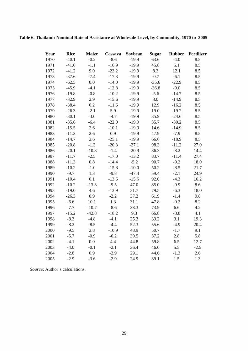
29

Table 6. Thailand: Nominal Rate of Assistance at Wholesale Level, by Commodity, 1970 to 2005

Year Rice Maize Cassava Soybean Sugar Rubber Fertilizer 1970 -40.1 -0.2 -8.6 -19.9 63.6 -4.0 8.5 1971 -41.0 -1.1 -16.9 -19.9 45.8 5.1 8.5 1972 -41.2 9.0 -23.2 -19.9 8.3 12.1 8.5 1973 -37.6 -7.4 -17.3 -19.9 -0.7 -6.1 8.5 1974 -62.5 0.0 -14.0 -19.9 -35.6 -22.9 8.5 1975 -45.9 -4.1 -12.8 -19.9 -36.8 -9.0 8.5 1976 -19.8 -0.8 -10.2 -19.9 -5.6 -14.7 8.5 1977 -32.9 2.9 -15.6 -19.9 3.0 -14.9 8.5 1978 -38.4 0.2 -11.6 -19.9 12.9 -16.2 8.5 1979 -26.3 -2.1 5.9 -19.9 19.0 -19.2 8.5 1980 -30.1 -3.0 -4.7 -19.9 35.9 -24.6 8.5 1981 -35.6 -6.4 -22.0 -19.9 35.7 -30.2 8.5 1982 -15.5 2.6 -10.1 -19.9 14.6 -14.9 8.5 1983 -11.3 2.6 0.9 -19.9 47.9 -7.9 8.5 1984 -14.7 2.6 -25.1 -19.9 66.6 -18.9 8.5 1985 -20.8 -1.3 -20.3 -27.1 98.3 -11.2 27.0 1986 -20.1 -10.8 -1.4 -20.9 86.3 -8.2 14.4 1987 -11.7 -2.5 -17.0 -13.2 83.7 -11.4 27.4 1988 -11.3 0.8 -14.4 -5.2 90.7 -9.2 18.0 1989 -10.2 -1.0 -15.8 -10.0 50.2 -8.5 21.7 1990 -9.7 1.3 -9.8 -47.4 59.4 -2.1 24.9 1991 -10.4 0.1 -13.6 -15.6 92.0 -4.3 16.2 1992 -10.2 -13.3 -9.5 47.0 85.0 -0.9 8.6 1993 -19.0 4.6 -13.9 31.7 79.5 -6.3 18.0 1994 -26.3 0.9 -2.2 37.2 61.9 -1.4 9.8 1995 -6.6 10.1 1.3 31.1 47.8 -0.2 8.2 1996 -7.7 -10.7 -8.6 33.3 73.9 6.6 4.2 1997 -15.2 -42.8 -18.2 9.3 66.8 -8.8 4.1 1998 -8.3 -4.8 -4.1 25.3 33.2 3.1 19.3 1999 -8.2 -8.5 -4.4 52.3 55.6 -4.9 20.4 2000 -9.5 2.8 -10.9 48.9 50.7 -1.7 9.1 2001 -5.7 -0.9 -6.2 39.5 37.2 2.8 5.8 2002 -4.1 0.0 4.4 44.8 59.8 6.5 12.7 2003 -4.0 -0.1 -2.1 36.4 46.0 5.5 -2.5 2004 -2.8 0.9 -2.9 29.1 44.6 -1.3 2.6 2005 -2.9 -3.6 -2.9 24.9 39.1 1.5 1.3

Source: Author’s calculations.

30

Table 7. Thailand: Estimates of Transmission Elasticities from Wholesale to Farm Prices

Commodity Estimated elasticity

(t-statistic)

Rice

0.7587

(7.30)

Maize

0.8089

(14.38)

Cassava

1.0695

(8.20)

Soybeans

0.8003

(11.23)

Sugar

0.5309

(3.93)

Palm oil

[0.8981] a

(19.97)

Rubber

0.8981

(19.97)

Fertilizer

0.8889

(17.70)

Source: Author’s calculations, using data and methodology discussed in the text. Estimates shown relate to the parameter ib in equation (2). Note: t-statistics are shown in parthentheses. a Estimation for palm oil was not possible, due to insufficient data points, and the estimated value for rubber was used instead.

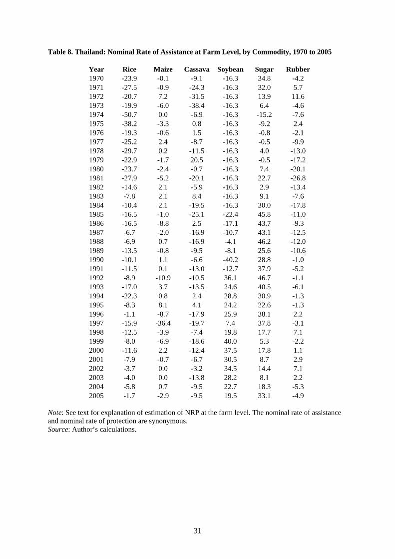
31

Table 8. Thailand: Nominal Rate of Assistance at Farm Level, by Commodity, 1970 to 2005

Year Rice Maize Cassava Soybean Sugar Rubber 1970 -23.9 -0.1 -9.1 -16.3 34.8 -4.2 1971 -27.5 -0.9 -24.3 -16.3 32.0 5.7 1972 -20.7 7.2 -31.5 -16.3 13.9 11.6 1973 -19.9 -6.0 -38.4 -16.3 6.4 -4.6 1974 -50.7 0.0 -6.9 -16.3 -15.2 -7.6 1975 -38.2 -3.3 0.8 -16.3 -9.2 2.4 1976 -19.3 -0.6 1.5 -16.3 -0.8 -2.1 1977 -25.2 2.4 -8.7 -16.3 -0.5 -9.9 1978 -29.7 0.2 -11.5 -16.3 4.0 -13.0 1979 -22.9 -1.7 20.5 -16.3 -0.5 -17.2 1980 -23.7 -2.4 -0.7 -16.3 7.4 -20.1 1981 -27.9 -5.2 -20.1 -16.3 22.7 -26.8 1982 -14.6 2.1 -5.9 -16.3 2.9 -13.4 1983 -7.8 2.1 8.4 -16.3 9.1 -7.6 1984 -10.4 2.1 -19.5 -16.3 30.0 -17.8 1985 -16.5 -1.0 -25.1 -22.4 45.8 -11.0 1986 -16.5 -8.8 2.5 -17.1 43.7 -9.3 1987 -6.7 -2.0 -16.9 -10.7 43.1 -12.5 1988 -6.9 0.7 -16.9 -4.1 46.2 -12.0 1989 -13.5 -0.8 -9.5 -8.1 25.6 -10.6 1990 -10.1 1.1 -6.6 -40.2 28.8 -1.0 1991 -11.5 0.1 -13.0 -12.7 37.9 -5.2 1992 -8.9 -10.9 -10.5 36.1 46.7 -1.1 1993 -17.0 3.7 -13.5 24.6 40.5 -6.1 1994 -22.3 0.8 2.4 28.8 30.9 -1.3 1995 -8.3 8.1 4.1 24.2 22.6 -1.3 1996 -1.1 -8.7 -17.9 25.9 38.1 2.2 1997 -15.9 -36.4 -19.7 7.4 37.8 -3.1 1998 -12.5 -3.9 -7.4 19.8 17.7 7.1 1999 -8.0 -6.9 -18.6 40.0 5.3 -2.2 2000 -11.6 2.2 -12.4 37.5 17.8 1.1 2001 -7.9 -0.7 -6.7 30.5 8.7 2.9 2002 -3.7 0.0 -3.2 34.5 14.4 7.1 2003 -4.0 0.0 -13.8 28.2 8.1 2.2 2004 -5.8 0.7 -9.5 22.7 18.3 -5.3 2005 -1.7 -2.9 -9.5 19.5 33.1 -4.9

Note: See text for explanation of estimation of NRP at the farm level. The nominal rate of assistance and nominal rate of protection are synonymous. Source: Author’s calculations.

32

Table 9. Thailand: Direct Rate of Assistance at Farm Level, by Commodity, 1970 to 2005

Year Rice Maize Cassava Soybean Sugar Rubber 1970 -24.9 -2.5 -10.1 -17.3 33.0 -5.0 1971 -28.4 -3.2 -25.3 -17.3 30.1 4.9 1972 -21.6 4.9 -32.6 -17.4 12.1 10.9 1973 -20.7 -8.2 -39.5 -17.5 4.6 -5.3 1974 -51.7 -2.2 -8.0 -17.5 -17.0 -8.3 1975 -39.0 -5.4 -0.4 -17.6 -11.0 1.7 1976 -19.9 -2.7 0.2 -17.6 -2.6 -2.8 1977 -25.8 0.4 -10.1 -17.7 -2.4 -10.6 1978 -30.3 -1.8 -12.9 -17.7 2.1 -13.7 1979 -23.3 -3.6 19.1 -17.8 -2.3 -18.0 1980 -24.1 -4.3 -2.2 -17.8 5.6 -20.8 1981 -28.4 -7.1 -21.6 -17.8 20.9 -27.6 1982 -15.0 0.2 -7.4 -17.8 1.2 -14.1 1983 -8.2 0.1 7.0 -17.8 7.5 -8.4 1984 -10.8 0.1 -20.8 -17.8 28.5 -18.7 1985 -19.5 -7.5 -29.3 -27.3 40.9 -13.8 1986 -17.8 -12.2 0.2 -19.6 41.0 -10.8 1987 -9.7 -8.5 -21.3 -15.5 38.0 -15.3 1988 -8.6 -3.6 -19.7 -7.2 42.8 -13.8 1989 -15.8 -6.0 -13.0 -11.7 21.4 -12.8 1990 -12.9 -4.8 -10.6 -44.3 23.9 -3.5 1991 -13.0 -3.6 -15.6 -15.5 34.8 -6.8 1992 -9.4 -12.8 -12.0 34.6 45.1 -1.9 1993 -19.0 -0.1 -16.6 21.1 37.1 -7.6 1994 -23.2 -1.3 0.6 26.8 29.2 -2.1 1995 -8.7 6.5 2.6 22.4 21.1 -1.9 1996 -0.9 -9.5 -18.7 25.0 37.3 1.8 1997 -15.9 -37.1 -20.4 6.6 37.1 -3.6 1998 -14.9 -7.1 -10.6 16.5 14.5 4.1 1999 -10.7 -10.2 -22.0 36.8 1.9 -5.9 2000 -12.4 0.9 -13.9 36.2 16.3 -0.8 2001 -8.1 -1.5 -7.6 29.8 7.8 1.5 2002 -5.2 -1.7 -5.1 33.0 12.4 3.7 2003 -2.7 0.3 -13.4 28.4 8.5 2.9 2004 -5.5 0.4 -9.9 22.5 17.9 -6.1 2005 -1.2 -3.0 -9.7 19.4 32.9 -5.4

Note: DRA means the nominal rate of assistance at the farm level for that industry (Table 11) minus the product of the cost share of fertilizer for that industry and the nominal rate of assistance to fertilizer (Table 10). Source: Author’s calculations.

33

Table 10. Thailand: Aggregate Direct and Total Rates of Agricultural Assistance and Anti-trade Bias, 1970 to 2005

Direct Rates of Assistance Year

Total agriculture

(1)

Import agriculture

(2)

Export agriculture

(3)

Manu- facturing

(4)

Total rate of

assistance to agriculture

(5) 1970 -4.9 n.a. -4.9 32.9 -37.8 1971 -6.9 n.a. -6.9 32.9 -39.8 1972 -7.5 n.a. -7.5 32.9 -40.5 1973 -14.7 n.a. -14.7 32.9 -47.6 1974 -17.5 n.a. -17.5 32.9 -50.5 1975 -11.9 n.a. -11.9 32.9 -44.8 1976 -7.6 n.a. -7.6 32.9 -40.6 1977 -11.3 n.a. -11.3 32.9 -44.3 1978 -12.7 n.a. -12.7 32.9 -45.7 1979 -8.0 n.a. -8.0 32.9 -40.9 1980 -11.1 n.a. -11.1 32.9 -44.0 1981 -14.4 n.a. -14.4 32.9 -47.4 1982 -9.3 n.a. -9.3 32.9 -42.2 1983 -3.7 n.a. -3.7 32.9 -36.6 1984 -7.6 n.a. -7.6 32.9 -40.6 1985 -10.5 n.a. -10.5 32.9 -43.4 1986 -4.1 n.a. -4.1 32.9 -37.0 1987 -6.2 n.a. -6.2 32.9 -39.1 1988 -2.5 n.a. -2.5 32.9 -35.5 1989 -6.8 -11.7 -5.9 32.9 -39.7 1990 -8.7 -44.3 -1.9 33.9 -42.6 1991 -3.7 n.a. -3.7 32.9 -36.6 1992 7.0 12.7 4.5 34.1 -27.1 1993 1.7 21.1 -2.1 36.0 -34.3 1994 4.5 26.8 0.0 35.9 -31.4 1995 6.5 15.1 2.7 14.9 -8.4 1996 5.7 8.9 4.3 14.7 -9.0 1997 -5.3 -14.3 -1.4 14.3 -19.6 1998 0.3 4.9 -1.7 13.6 -13.3 1999 -2.4 13.3 -9.0 15.0 -17.4 2000 3.4 18.1 -2.7 9.7 -6.3 2001 2.8 29.8 -1.5 10.3 -7.5 2002 5.3 33.0 1.0 10.6 -5.3 2003 3.2 28.4 -0.5 10.6 -7.4 2004 1.9 22.5 -1.0 10.6 -8.7 2005 4.3 6.5 3.5 10.6 -6.3

Source: Author’s calculations.

34

Figure 1. Indonesia: Border and domestic prices of rice (Rp/kg), relative to the GDP deflator

(2005=1)

0500

100015002000250030003500400045005000

1975

1978

1981

1984

1987

1990

1993

1996

1999

2002

2005

-50.0

-40.0

-30.0

-20.0

-10.0

0.0

10.0

20.0

30.0

40.0

Border priceDomestic priceNRP (%)

Real price NRP

Left axis:

Right axis:

Source: Author’s calculations.

35

Figure 2. Indonesia: Border and domestic prices of sugar relative to the GDP deflator (2005=1)

0

1000

2000

3000

4000

5000

6000

700019

71

1974

1977

1980

1983

1986

1989

1992

1995

1998

2001

2004

-20

30

80

130

180

230

280

330

380

Border priceDomestic priceNRP (%)

Real price NRP

Left axis:

Right axis:

Source: Author’s calculations.

36

Figure 3. Indonesia: Border and domestic prices of urea fertiliser (Rp/kg), relative to the GDP

deflator (2005=1)

0

1000

2000

3000

4000

5000

1975

1978

1981

1984

1987

1990

1993

1996

1999

2002

-80.0

-60.0

-40.0

-20.0

0.0

20.0

40.0

Border priceDomestic priceNRP (%)smoothed NRP

Real price NRP

Left axis:

Right axis:

Source: Author’s calculations.

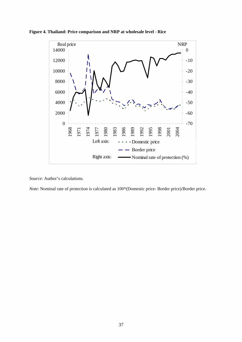
37

Figure 4. Thailand: Price comparison and NRP at wholesale level - Rice

0

2000

4000

6000

8000

10000

12000

14000

1968

1971

1974

1977

1980

1983

1986

1989

1992

1995

1998

2001

2004

-70

-60

-50

-40

-30

-20

-10

0

Domestic priceBorder priceNominal rate of protection (%)

Left axis:

Right axis:

Real price NRP

Source: Author’s calculations. Note: Nominal rate of protection is calculated as 100*(Domestic price- Border price)/Border price.

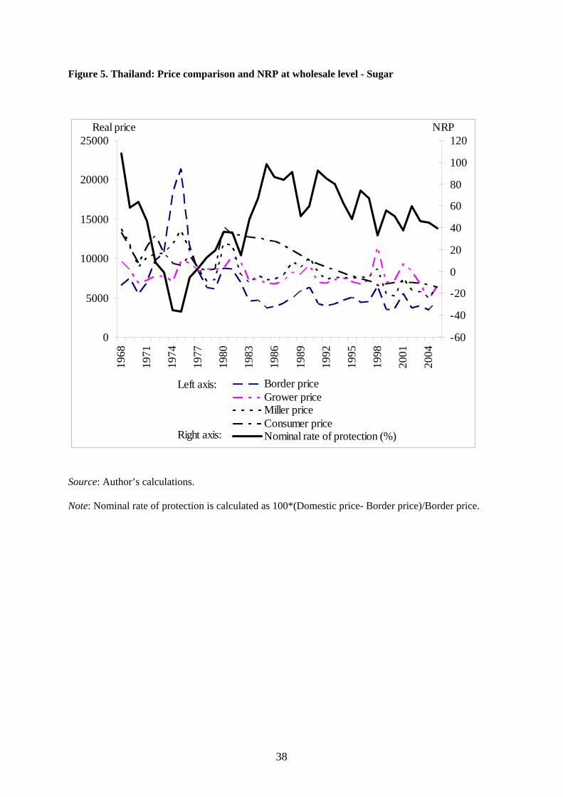
38

Figure 5. Thailand: Price comparison and NRP at wholesale level - Sugar

0

5000

10000

15000

20000

25000

1968

1971

1974

1977

1980

1983

1986

1989

1992

1995

1998

2001

2004

-60

-40

-20

0

20

40

60

80

100

120

Border priceGrower priceMiller priceConsumer priceNominal rate of protection (%)

Left axis:

Right axis:

Real price NRP

Source: Author’s calculations. Note: Nominal rate of protection is calculated as 100*(Domestic price- Border price)/Border price.

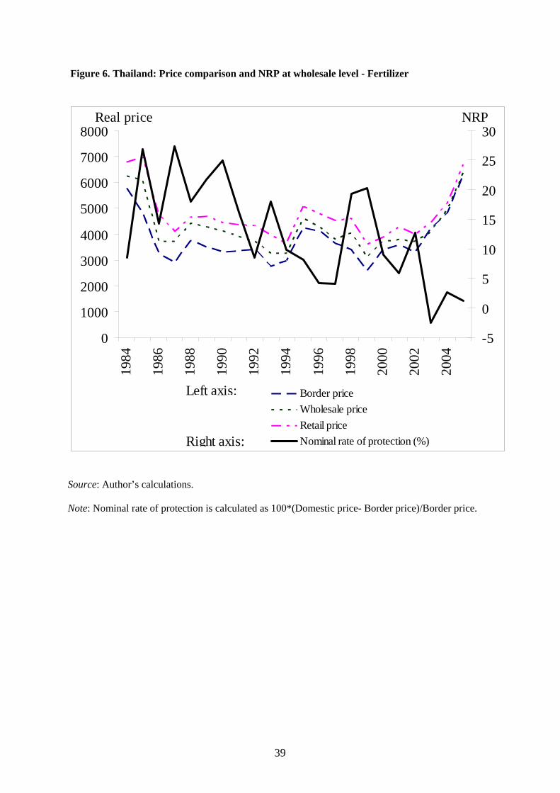
39

Figure 6. Thailand: Price comparison and NRP at wholesale level - Fertilizer

0

1000

2000

3000

4000

5000

6000

7000

800019

84

1986

1988

1990

1992

1994

1996

1998

2000

2002

2004

-5

0

5

10

15

20

25

30

Border priceWholesale priceRetail priceNominal rate of protection (%)

Left axis:

Right axis:

NRPReal price

Source: Author’s calculations. Note: Nominal rate of protection is calculated as 100*(Domestic price- Border price)/Border price.