THE EMERGENCE OF NEOCLASSICAL ECONOMICS

ECON 434 | Spring 2011

Alternatives to capitalism

Finishing up from last time

Alternatives to capitalism

Socialism Utopian Fabian Christian Revolutionary (Marxism)

Anarchism Syndicalism

Perspectives on libertarianism

http://www.huffingtonpost.com/2010/04/21/tea-partiers-in-tax-day-p_n_546909.html

http://www.youtube.com/watch?v=4kMxgOJK3-0&feature=fvw

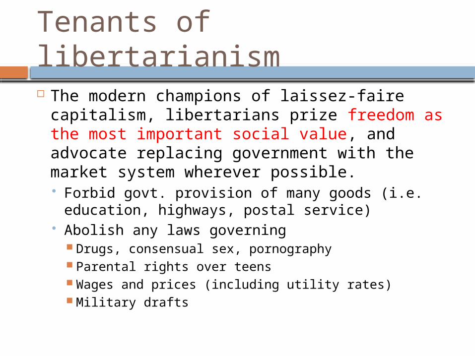
Tenants of libertarianism

The modern champions of laissez-faire capitalism, libertarians prize freedom as the most important social value, and advocate replacing government with the market system wherever possible. Forbid govt. provision of many goods (i.e.

education, highways, postal service) Abolish any laws governing

Drugs, consensual sex, pornography Parental rights over teens Wages and prices (including utility rates) Military drafts

Scandinavian welfare states

In modern welfare states, resources are largely privately owned, but high taxes and a massive welfare system mean that income is distributed across the society much more equally than, for example, in the United States.

“Welfare capitalism”

Buddhist economics

The idea that "small is beautiful" stresses curbing material want as the key to dealing with scarcity, and emphasizes local self-sufficiency, and small-scale, labor-intensive technology.

Drawn from Buddhist and Hindu religious thought

Intellectual foundations from Gandhi and E.F. Schumacher (Small is Beautiful: Economics as if People Mattered)

Neoclassical economics

The marginalist revolution

Application of mathematical analysis to economics begins in the mid 19th century This new methodological approach

distinguishes classical economics from neoclassical economics.

The use of formal mathematics was absent from Adam Smith’s works, for example

What is a marginal unit? What does it mean for a decision to be made “at the margin”?

The marginalist revolution cont. Marginal decisions are an incremental process Microeconomic analysis is based on

optimization, which entails weighing marginal benefits and marginal costs. Individuals maximize utility; firms, profits

A marginal unit is the extra (or last) unit. In a class of 20 students, all students, technically,

are the marginal student (if any student were to drop the course, 19 students would be enrolled).

Marginal changes are typically denoted with the Greek symbol delta (ΔP reads “change in price”)

Marginal analysis

(Q*, P*) optimizes individual utility (MC = MB) To the left of Q* = Individual hasn’t consumed enough To the right of Q* = Individual has consumed too much

MC

MB

P*

Q*

Marginal analysis cont.

The law of equal marginal advantage requires equivalent goods or similar resources to be allocated in equally advantageous ways at the margin. Mathematically, we can write MUx/Px = MUy/Py = …

Suppose that you and your identical twin are equally strong, experienced, and intelligent. If your twin works an 8-hour day and produces $64 worth of mowed lawns while you generate $48 worth of cleaned windows with similar effort, something is wrong. You will (and should) shift into mowing lawns so that your labor resources are allocated equally advantageously, at $8 per hour instead of the $6 per hour you have been earning.

Marginal analysis cont.

Would you eat less from a menu where prices are a la carte or where fixed price is charged for a buffet?

You probably eat less from a menu where prices are a la carte than if a restaurant charges a fixed price for a buffet; “all-you-can-eat” pricing causes you to view the cost of extra food as zero.

Marginal analysis cont.

Other examples of marginal analysis in economics: People's time must be divided between work and

leisure so that the gain in income from the last hour an individual works (the individual's wage) just equals the subjective value of the last hour of leisure enjoyed.

The last dollar a firm pays for labor must generate the same amount of extra production (and profit) as the last dollar spent on capital or land.

The dollar value to a consumer of the right to consume a particular good must equal the value of other production that society sacrifices in making that marginal unit of the good available to that consumer.

Calculus and marginal analysis Isaac Newton and Gottfried Wilhelm von

Leibniz independently discover calculus around 1675.

Takes over 170 years before calculus is applied to economics.

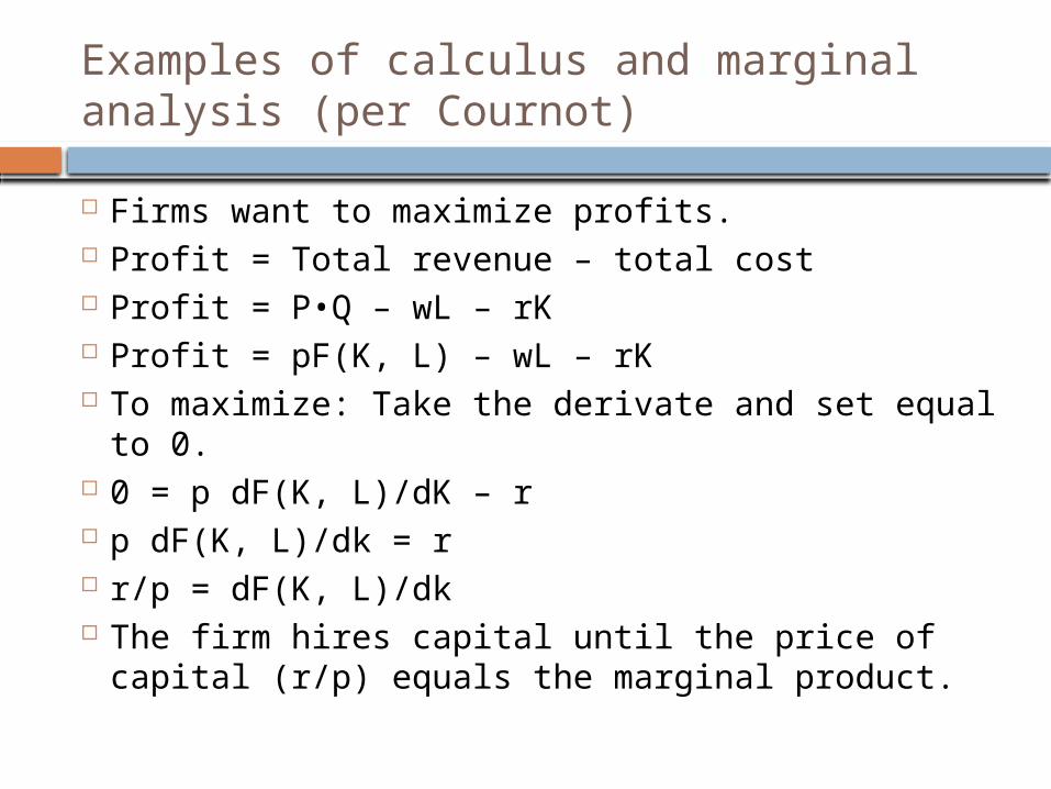
Examples of calculus and marginal analysis (per Cournot)

Firms want to maximize profits. Profit = Total revenue – total cost Profit = P•Q – wL – rK Profit = pF(K, L) – wL – rK To maximize: Take the derivate and set equal to 0. 0 = p dF(K, L)/dK – r p dF(K, L)/dk = r r/p = dF(K, L)/dk The firm hires capital until the price of capital (r/p)

equals the marginal product.

Early foundations of marginalism

W. S. Jevons (1835-1882) “Bygones are forever

bygones” Sunk costs are irrelevant

for future decisions. Example: Waiting in line

Diamond-water paradox and marginal pricing

W.S. Jevons cont.

Theory of Political Economy (1871) Diminishing marginal utility Equimarginal principle

Sunspot theory and the beginnings of econometrics

Prices are determined by supply and demand Contrast with classical assumption that

demand is always adequate Say’s law: Supply creates its own demand

Forerunners of marginal analysis

Jules Dupuit Price discrimination: Occurs when virtually

identical units of a good are sold at different prices, and price differentials do not reflect different production costs. Popular examples include movie tickets (i.e., different

prices for teens, senior citizens) and coupons Requirements for price discrimination

The firm must have some amount of market power The firm must know the demand schedule (the

consumers’ willingness to pay) The firm must be able to prevent resale (arbitrage)

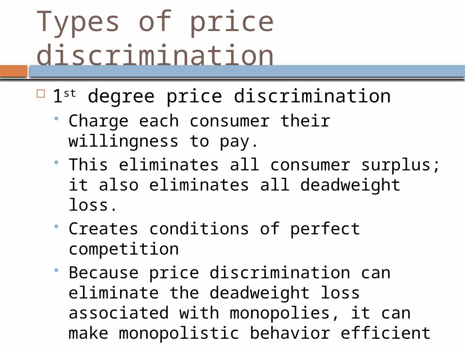
Types of price discrimination 1st degree price discrimination

Charge each consumer their willingness to pay.

This eliminates all consumer surplus; it also eliminates all deadweight loss.

Creates conditions of perfect competition Because price discrimination can eliminate

the deadweight loss associated with monopolies, it can make monopolistic behavior efficient

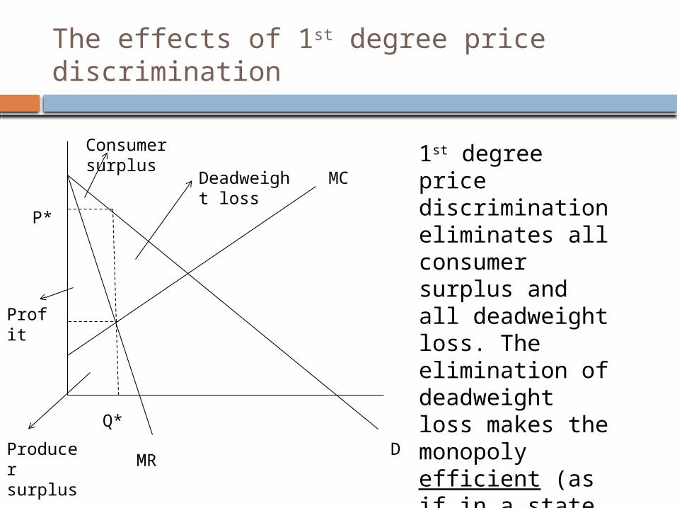
The effects of 1st degree price discrimination

MC

DMR

P*

Q*

Producer surplus

Profit

Consumer surplus

Deadweight loss

1st degree price discrimination eliminates all consumer surplus and all deadweight loss. The elimination of deadweight loss makes the monopoly efficient (as if in a state of perfect competition).

A monopoly with 1st degree price discrimination

Price discrimination on a person-by-person basis where each is charged the most they are willing to pay (the firm knows each person’s demand curve)

Marginal revenue = demand No consumer surplus; all producer surplus

MC

D

Price discrimination cont.

2nd degree price discrimination: Charge different per unit prices for different amounts of a good for strategic reasons Bulk discounts Block pricing: first bunch of goods you buy is

expensive; the next bunch is less expensive 3rd degree price discrimination: Charge each

group of consumers a different price based on their willingness to pay Classify individuals into groups and charge all

they will bear

Forerunners of marginal analysis

A.A. Cournot First to clearly define a demand curve

mathematically Profit maximizing rule: MR = MC Employs calculus for optimization problems

(see the “Examples of Calculus in Marginal Analysis” slide)

Distinguishes changes in demand from changes in quantity demanded

A.A. Cournot

Distinguishes changes in demand from changes in quantity demanded

P

Q

D1

D0

S0

P

Q

S0

D0

S1

Change in demand Change in quantity demanded

Cournot duopoly model

Sets the foundation for modern game theory

Two firms strategically choose their output (quantity-adjusting model)

P = a – bq Marginal cost = c(q) Profit firm x(q1, q2) = p*qx – c(qx) Profit firm 1(q1, q2) = q1[a – b(q1 + q2)] –

c(q1) Profit firm 2(q1, q2) = q2[a – b(q1 + q2)] –

c(q2)

Cournot duopoly model

Profit firm 1(q1, q2) = q1[a – b(q1 + q2)] – c(q1)

Re-write the equation: q1[a – bq1 – bq2] – c(q1)

Re-write the equation: q1a – bq12 – bq1q2 – c(q1) 0 = aq1 – bq12 – bq1q2 – c(q1) 0 = a – 2bq1 – bq2 – c 2bq1 = a – bq2 – c Q1 = (a – bq2 – c)/(2b)

This is firm one’s best response function.

Cournot duopoly model

The point: The quantity at which a firm decides to produce is dependent upon the quantity (and subsequent quantity adjustments) of another firm

Assumes continuous strategic interaction between firms

Compare to Bertrand, who said that firms would adjust prices This anticipates a larger debate between

Keynesians and traditional macroeconomists