The elemental composition of the Sun - McGill Physicspatscott/publications/1405.0288v1.pdf · The...
24
Astronomy & Astrophysics manuscript no. Neutron˙capture-print˙format c ESO 2014 May 5, 2014 The elemental composition of the Sun III. The neutron capture elements Cu to Th Nicolas Grevesse 1,2 , Pat Scott 3 , Martin Asplund 4 , and A. Jacques Sauval 5 1 Centre Spatial de Li` ege, Universit´ e de Li` ege, avenue Pr´ e Aily, B-4031 Angleur-Li` ege, Belgium 2 Institut d’Astrophysique et de G´ eophysique, Universit´ e de Li` ege, All´ ee du 6 ao ˆ ut, 17, B5C, B-4000 Li` ege, Belgium e-mail: [email protected] 3 Department of Physics, Imperial College London, Blackett Laboratory, Prince Consort Road, London SW7 2AZ, UK e-mail: [email protected] 4 Research School of Astronomy and Astrophysics, Australian National University, Cotter Rd., Weston Creek, ACT 2611, Australia e-mail: [email protected] 5 Observatoire Royal de Belgique, avenue circulaire, 3, B-1180 Bruxelles, Belgium e-mail: [email protected] Received Day Month Year / Accepted Day Month Year ABSTRACT We re-evaluate the abundances of the elements in the Sun from copper (Z = 29) to thorium (Z = 90). Our results are mostly based on neutral and singly-ionised lines in the solar spectrum. We use the latest 3D hydrodynamic solar model atmosphere, and in a few cases also correct for departures from local thermodynamic equilibrium (NLTE). In order to minimise statistical and systematic uncertainties, we make stringent line selections, employ the highest-quality observational data and carefully assess oscillator strengths, hyperfine constants and isotopic separations available in the literature, for every line included in our analysis. Our results are typically in good agreement with the abundances in the most pristine meteorites, but there are some interesting exceptions. This analysis constitutes both a full exposition and a slight update of the relevant parts of the preliminary results we presented in Asplund, Grevesse, Sauval & Scott (2009), including full line lists and details of all input data that we have employed. Key words. Sun: abundances – Sun: photosphere – Sun: granulation – Line: formation – Line: profiles – Convection 1. Introduction Due to the Coulomb barrier and the fact that nuclear binding en- ergy peaks at iron, the elements beyond the Fe-peak (Z ≥ 29, i.e. Cu and heavier elements) are not produced by exothermic charged-particle fusion reactions in stable nuclear burning in- side stars. Instead, these elements are forged by successive neu- tron capture followed by β-decay. 1 There are two main chan- nels through which the isotopes of the heavy elements are pro- duced: slow and rapid neutron capture (the s- and r-processes, respectively). The distinction between s and r depends on the neutron density, such that the timescale for β-decay is shorter ( s-process) or longer (r-process) than the timescale for neutron capture. Once the neutron flux recedes, the neutron-rich isotopes from the r-process decay back to the valley of stability (Burbidge et al. 1957; Cameron 1957). As a result, most elements have a mixed origin, although a few isotopes and elements are produced almost exclusively by one or the other neutron-capture process (e.g. Sneden et al. 2008). Roughly half of the isotopes come pri- marily from the s-process and the other half from the r-process (see Table 3 in Anders & Grevesse 1989, for a full inventory). Observationally, the neutron capture elements show large abun- 1 Even though their nuclear origins are mixed, we include Cu and Zn in this study together with the neutron-capture elements. For example, roughly half of the solar Zn was produced in nuclear statistical equilib- rium (creating 64 Zn), possibly in connection with hypernovae (highly energetic core-collapse supernovae). The neutron-rich isotopes of Zn however stem from neutron capture (e.g. Kobayashi & Nakasoto 2011). dance variations between stars, especially at low metallicity (e.g. Roederer et al. 2014). The r-process produces abundance peaks mainly at Z ≈ 32, 54 and 78 (Ge, Xe and Pt), whereas a typical s-process abundance pattern has peaks at Z ≈ 38, 56 and 82 (Sr, Ba and Pb). The main site of the s-process is believed to be thermally pulsing asymptotic giant branch (AGB) stars (e.g. Sneden et al. 2008). The main neutron source in these stars is thought to be 13 C(α,n) 16 O, although 22 Ne(α,n) 25 Mg can also operate, es- pecially in more massive AGB stars (e.g. Busso et al. 2001; Karakas et al. 2012). More recently, it has been realised that the s-process can also be efficient in rapidly-rotating massive stars at low metallicity, through the production of primary N later con- verted to 22 Ne (Pignatari et al. 2008). The site(s) of the r-process have not yet been unanimously agreed upon. Numerous possibilities have been proposed, none altogether convincing. Currently the main contenders are core- collapse supernovae (e.g. in connection with a neutrino wind, Wanajo 2013) or mergers of neutron stars with either black holes or other neutron stars (Goriely et al. 2011), but achieving the necessary neutron fluxes and entropies is challenging in either case. A handful of stars at low metallicity are strongly enriched in the r-process elements, with an abundance pattern remarkably similar to the r-process signature in the solar system, suggesting the dominance of some universal process active throughout cos- mic time (e.g. Cayrel et al. 2001, Sneden et al. 2003, Frebel et al. 2007). In a few cases, the r-process enhancement is so high that it has enabled the detection of radioactive elements like tho- 1 arXiv:1405.0288v1 [astro-ph.SR] 1 May 2014
Transcript of The elemental composition of the Sun - McGill Physicspatscott/publications/1405.0288v1.pdf · The...
Astronomy & Astrophysics manuscript no. Neutron˙capture-print˙format c© ESO 2014May 5, 2014
The elemental composition of the SunIII. The neutron capture elements Cu to Th
Nicolas Grevesse1,2, Pat Scott3, Martin Asplund4, and A. Jacques Sauval5
1 Centre Spatial de Liege, Universite de Liege, avenue Pre Aily, B-4031 Angleur-Liege, Belgium2 Institut d’Astrophysique et de Geophysique, Universite de Liege, Allee du 6 aout, 17, B5C, B-4000 Liege, Belgium
e-mail: [email protected] Department of Physics, Imperial College London, Blackett Laboratory, Prince Consort Road, London SW7 2AZ, UK
e-mail: [email protected] Research School of Astronomy and Astrophysics, Australian National University, Cotter Rd., Weston Creek, ACT 2611, Australia
e-mail: [email protected] Observatoire Royal de Belgique, avenue circulaire, 3, B-1180 Bruxelles, Belgium
e-mail: [email protected]
Received Day Month Year / Accepted Day Month Year
ABSTRACT
We re-evaluate the abundances of the elements in the Sun from copper (Z = 29) to thorium (Z = 90). Our results are mostly basedon neutral and singly-ionised lines in the solar spectrum. We use the latest 3D hydrodynamic solar model atmosphere, and in afew cases also correct for departures from local thermodynamic equilibrium (NLTE). In order to minimise statistical and systematicuncertainties, we make stringent line selections, employ the highest-quality observational data and carefully assess oscillator strengths,hyperfine constants and isotopic separations available in the literature, for every line included in our analysis. Our results are typicallyin good agreement with the abundances in the most pristine meteorites, but there are some interesting exceptions. This analysisconstitutes both a full exposition and a slight update of the relevant parts of the preliminary results we presented in Asplund, Grevesse,Sauval & Scott (2009), including full line lists and details of all input data that we have employed.
Key words. Sun: abundances – Sun: photosphere – Sun: granulation – Line: formation – Line: profiles – Convection
1. Introduction
Due to the Coulomb barrier and the fact that nuclear binding en-ergy peaks at iron, the elements beyond the Fe-peak (Z ≥ 29,i.e. Cu and heavier elements) are not produced by exothermiccharged-particle fusion reactions in stable nuclear burning in-side stars. Instead, these elements are forged by successive neu-tron capture followed by β-decay.1 There are two main chan-nels through which the isotopes of the heavy elements are pro-duced: slow and rapid neutron capture (the s- and r-processes,respectively). The distinction between s and r depends on theneutron density, such that the timescale for β-decay is shorter(s-process) or longer (r-process) than the timescale for neutroncapture. Once the neutron flux recedes, the neutron-rich isotopesfrom the r-process decay back to the valley of stability (Burbidgeet al. 1957; Cameron 1957). As a result, most elements have amixed origin, although a few isotopes and elements are producedalmost exclusively by one or the other neutron-capture process(e.g. Sneden et al. 2008). Roughly half of the isotopes come pri-marily from the s-process and the other half from the r-process(see Table 3 in Anders & Grevesse 1989, for a full inventory).Observationally, the neutron capture elements show large abun-
1 Even though their nuclear origins are mixed, we include Cu and Znin this study together with the neutron-capture elements. For example,roughly half of the solar Zn was produced in nuclear statistical equilib-rium (creating 64Zn), possibly in connection with hypernovae (highlyenergetic core-collapse supernovae). The neutron-rich isotopes of Znhowever stem from neutron capture (e.g. Kobayashi & Nakasoto 2011).
dance variations between stars, especially at low metallicity (e.g.Roederer et al. 2014). The r-process produces abundance peaksmainly at Z ≈ 32, 54 and 78 (Ge, Xe and Pt), whereas a typicals-process abundance pattern has peaks at Z ≈ 38, 56 and 82 (Sr,Ba and Pb).
The main site of the s-process is believed to be thermallypulsing asymptotic giant branch (AGB) stars (e.g. Sneden etal. 2008). The main neutron source in these stars is thought tobe 13C(α,n)16O, although 22Ne(α,n)25Mg can also operate, es-pecially in more massive AGB stars (e.g. Busso et al. 2001;Karakas et al. 2012). More recently, it has been realised that thes-process can also be efficient in rapidly-rotating massive stars atlow metallicity, through the production of primary N later con-verted to 22Ne (Pignatari et al. 2008).
The site(s) of the r-process have not yet been unanimouslyagreed upon. Numerous possibilities have been proposed, nonealtogether convincing. Currently the main contenders are core-collapse supernovae (e.g. in connection with a neutrino wind,Wanajo 2013) or mergers of neutron stars with either black holesor other neutron stars (Goriely et al. 2011), but achieving thenecessary neutron fluxes and entropies is challenging in eithercase. A handful of stars at low metallicity are strongly enrichedin the r-process elements, with an abundance pattern remarkablysimilar to the r-process signature in the solar system, suggestingthe dominance of some universal process active throughout cos-mic time (e.g. Cayrel et al. 2001, Sneden et al. 2003, Frebel etal. 2007). In a few cases, the r-process enhancement is so highthat it has enabled the detection of radioactive elements like tho-
1
arX
iv:1
405.
0288
v1 [
astr
o-ph
.SR
] 1
May
201
4
Grevesse et al.: Solar abundances III. The neutron capture elements (Cu to Th)
rium and uranium in the stellar spectra, which has made age-dating of the nucleosynthesis sites possible (cosmo-chronology,Butcher 1987). Because the r-process elements can have a pri-mary origin (being produced from Fe-nuclei seeds) in contrastto the secondary origin of the s-process elements (which requirefirst the production of 13C or 22Ne nuclei as neutron sources), ther-process should dominate in the early Universe (Truran 1981).
A proper understanding of the nuclear processes involved inthe production of the heavy elements requires a detailed knowl-edge of the solar system abundances. In a recent review (Asplundet al. 2009: AGSS09), we presented a summary of our redetermi-nation of nearly all available elements in the solar photosphere.In this work (Paper III), we give detailed and homogeneous re-sults for the elements Cu to Th, updating AGSS09 where nec-essary. We use the most recent 3D atmospheric model togetherwith the best atomic and solar data. Previous papers in this serieshave focussed on Na – Ca (Scott et al. 2014a: Paper I) and theFe group (Scott et al. 2014b: Paper II) with remaining elementsto be dealt with in future studies. Amongst the heavy elements,so far zirconium (Ljung et al. 2006; Caffau et al. 2011a), os-mium (Caffau et al. 2011b), europium (Mucciarelli et al. 2008),hafnium and thorium (Caffau et al. 2008) have been subjected to3D solar analysis.
Sect. 2 describes the observations we use and how we em-ploy them. Sect. 3 quickly recaps the salient details of the modelatmospheres used in this series, and Sect. 4 describes the atomicdata and NLTE corrections we have employed in this paper. InSect. 5 we give our abundance results for all elements, followedby a discussion of their dependence on the chosen model atmo-sphere in Sect. 6. We compare our results with some previouscompilations of the solar chemical composition for the heavyelements in Sect. 7, before concluding in Sect. 8.
2. Observations
We have employed the Jungfraujoch (Delbouille et al. 1973) andKitt Peak (visual: Neckel & Labs 1984; near-infrared: Delbouilleet al. 1981) disc-centre solar spectral atlases to carefully measurethe equivalent widths of a large number of lines of the elementsCu to Th. Wherever possible, we have been very demanding inthe quality of the lines we retained. We carefully examined theshape and full width of each line, to detect any trace of blend-ing lines. We gave each line a weight from 1 to 3, dependingon the uncertainty that we estimated for the measured equiva-lent width, factoring in potential pitfalls such as blends and con-tinuum placement. We integrated observed and theoretical lineprofiles over the same wavelength regions when measuring theequivalent widths.
For most of the elements we used the measured equivalentwidths to derive abundances with the new model atmosphere de-scribed in Sec. 3. In some cases however (Nb, rare earths, Hf,W), we instead update results obtained by other authors withspectral synthesis and the Holweger & Muller (1974) photo-spheric model, to account for the effect of the new 3D hydrody-namic solar model (Sect. 3). We included isotopic and hyperfinestructure of lines as a series of blending features, as described indetail in Paper I, using the adopted atomic data detailed belowfor each relevant species (Sect. 4).
3. Solar model atmospheres and spectral lineformation
We follow the same procedure as in Papers I and II. We use thenew 3D, time-dependent, hydrodynamic simulation of the so-
lar surface convection first employed in AGSS09 as a realisticmodel of the solar photosphere. The reader is referred to Paper I(Scott et al. 2014a) for further details of the 3D solar model. Asdemonstrated extensively by Pereira et al. (2013), this 3D modelperforms extremely well against an arsenal of key observationaltests, indicating that the model is highly realistic. In particular,we note that our 3D solar model perfectly predicts the continuumcentre-to-limb variation, which is a sensitive probe of the meantemperature structure in the typical line-forming region of thephotosphere. The corresponding theoretical absolute intensitiesagree extremely well with observations as well.
For comparison, and to quantify the systematic errors of ourabundance results, we have also again performed identical cal-culations with four different 1D models of the solar photosphere:the widely-used, hydrostatic, semi-empirical model of Holweger& Muller (1974; HM) which has been pressure-integrated tobe consistent with our continuous opacities and chemical com-positions, the mean 3D model 〈3D〉 obtained by spatially andtemporally averaging the 3D model over about 45 min of solartime, the solar model from the grid of marcs theoretical mod-els extensively used for abundance analysis of solar-type stars(Asplund et al. 1997, Gustafsson et al. 2008), and the miss semi-empirical model obtained from 1D LTE spectral inversion of Felines (Allende Prieto et al. 2001).
For all spectral line formation calculations we assumed localthermodynamic equilibrium (LTE). Non-LTE (NLTE) analysesperformed in a 1D framework for the Sun exist to our knowledgeonly for Cu i, Zn i, Sr i, Sr ii, Zr i, Zr ii, Ba ii, Eu ii, Pb i and Th ii(see below for individual references for each element). Whensuch NLTE data are available, we correct the 3D LTE and 1DLTE results with those NLTE abundance corrections. We notethat this is not fully self-consistent as the departures from LTEmay be different in 3D than in 1D, indeed often depending on theparticular 1D model atmosphere used. As a rule of thumb, NLTEeffects are more pronounced in theoretical model atmospheresthan in semi-empirical ones due to their steeper temperature gra-dients, a phenomenon dubbed ‘NLTE masking’ by Rutten &Kostik (1982). For completeness, we also mention that NLTEcalculations are often performed for flux spectra, but we employdisc-centre intensity spectra; NLTE effects tend to be less severein intensity than flux because the absorption lines are formed atlower heights in intensity than in flux. As is clear from the fewNLTE studies available, much work still remains to be done inthis area for the heavy elements. The shortage of NLTE investi-gations is partially due to the relatively small number of expertsin the field. For these elements however, perhaps the biggestreason for the dearth of NLTE analyses is a lack of necessaryatomic data such as photo-ionisation cross-sections, transitionprobabilities and collisional rates for the many relevant atomicprocesses in what are often highly complicated atoms (Asplund2005). NLTE calculations with incomplete model atoms and/orless precise atomic data can often be rather misleading – but socan LTE. The assumption of LTE is an extreme one, and not atall a cautious middle ground. Caution should therefore be exer-cised with elements lacking NLTE corrections. Fortunately, forthe heavy elements, in most cases we rely on lines from the dom-inant ionisation stage, which typically exhibit less severe depar-tures from LTE than minority species (Asplund 2005); in thesolar case the once-ionised species are typically in the majority.
As explained in Paper I, with a 3D solar model there is noneed to invoke any micro- or macroturbulent velocities to ob-tain correct line broadening (Asplund et al. 2000). For all 1Dmodels, we adopted a microturbulence of 1 km s−1. We carriedout 3D line formation calculations for 45 snapshots from the full
2
Grevesse et al.: Solar abundances III. The neutron capture elements (Cu to Th)
time sequence of the 3D solar model, spaced 1 min apart, andaveraged them before carrying out the continuum normalisation.
4. Atomic data and line selection
The atomic data (transition probabilities, isotopic structure andhyperfine structure: HFS) we adopt are discussed in detail belowfor each element. We give our adopted lines, oscillator strengths,NLTE corrections, equivalent widths, excitation potentials andderived abundances for all elements in Table 1, and isotopic andHFS data in Table 2. We have also re-examined the ionisationenergies and partition functions in detail, updating some data rel-ative to AGSS09; this is not trivial, as even many recent analysesare still based on quite erroneous data. These data are given inTable 3. For Ho ii our partition functions come from from Bord& Cowley (2002), and for all other species, from Barklem &Collet (in preparation); these are in good agreement with val-ues computed from NIST atomic energy levels. Our ionisationenergies come from the NIST data tables.
Modern line-broadening data for collisions with hydrogenatoms are available from Barklem, Piskunov & O’Mara (2000)for all the neutral lines we consider in this paper, but only Ba iiand Sr ii amongst the ionised lines. We use this data wherever itexists; otherwise, we use the classical recipe of Unsold (1955)with an enhancement factor of 2.0.
4.1. Copper
Although Cu is essentially once ionised in the solar photosphere,only Cu i lines have been identified in the solar spectrum. Fromthe works of Kock & Richter (1968) and Sneden & Crocker(1988), we retained the five Cu i lines given in Table 1. Forthe first three lines, we have used the experimental g f -valuesof Kock & Richter, renormalised to the lifetimes of Carlssonet al. (1989; the renormalisation amounts to a change of only−0.006 dex). For the last two lines, we took oscillator strengthsfrom Bielski (1975), based on the measurements of Meggers etal. (1961).
Cu is approximately 69.2% 63Cu and 30.8% 65Cu (AGSS09),both of which have nuclear spin I = 3
2 . The strongest solarlines are affected by isotopic broadening and HFS. We accountedfor isotopic splitting using the data of Fischer, Hunermann &Kollath (1967). We took HFS constants from the same paper aswell as from Hannaford & McDonald (1978).
NLTE Cu i line formation in the Sun was investigated byShi et al. (2014), who found positive NLTE corrections (≈+0.02 dex) for our first three lines, and a larger negative correc-tion (≈ −0.05 dex) for the last line (Cu i 809.3 nm). We adopttheir results for S H = 0.1, as recommended in their paper.Because the Cu i 793.3 nm and Cu i 809.3 nm lines differ onlyin the J values of their lower levels, and Shi et al. (2014) ex-plain the large negative NLTE offset in the abundance returnedby Cu i 809.3 nm as mainly due to underpopulation of the upperlevel of this transition, we assume that the NLTE correction forCu i 793.3 nm is the same as for Cu i 809.3 nm. The addition ofNLTE corrections for Cu i is a new feature of the analysis here,compared to AGSS09. We note that the NLTE study of Shi et al.is for flux rather than disc-centre intensity spectra, which meansthat the adopted NLTE effects may be slightly exaggerated.
4.2. Zinc
Zinc is mostly neutral in the photosphere. We retain the five Zn ilines given in Table 1. The g f -values we use come from Biemont& Godefroid (1980a), whose theoretical results agree well withmeasured lifetimes. For two lines (472.2 nm and 481.0 nm), werenormalise these data to the accurate lifetimes measured byKerkhoff et al. (1980) using laser spectroscopy, resulting in anincrease of 0.01 dex.
Y. Takeda (private communication, 2011) used the modelatom from Takeda et al. (2005) to compute NLTE correctionsof between −0.01 and −0.04 dex for our lines at the centre of thesolar disc, for different values of S H. For S H values between 0.1and 1 the NLTE corrections vary very little. We chose to use thecorrections at S H = 0.3.
4.3. Gallium
Although essentially once ionised, only the near-UV Ga i res-onance line at 417.2 nm (see Table 1) has been used by Ross& Aller (1970) and Lambert et al. (1969) to derive the solarGa abundance. This line is rather heavily perturbed and canonly be extracted by spectrum synthesis; doing so, these authorsfound εGa = 2.80 and εGa = 2.84 respectively. Lambert et al.also suggested using a very faint unidentified infrared line at1194.915 nm. They argued that this line could be due to Ga i,as in their analysis it led to an abundance in agreement withthe near-UV line. Oscillator strengths have been discussed byLambert et al., and we adopt their chosen value for the near-UV line. This comes from Cunningham & Link (1967), who seta theoretical branching fraction to an absolute scale with theirown accurate experimental lifetime.
We rechecked the IR line: it is suspiciously wide (suggestingunidentified blends), and its equivalent width is too inaccurateto keep as a good abundance indicator. We therefore synthesisedthe spectrum around the near-UV resonance line and derived anaccurate estimate of the Ga i contribution: 5.22±0.30 pm.
4.4. Germanium
Ge is also mostly once ionised in the solar photosphere, butonly very few Ge i lines have been identified. Accurate g f -valueshave been measured by Biemont et al. (1999). With the only us-able Ge i line (326.9 nm; Table 1), they applied their oscillatorstrength to derive a solar abundance of log εGe = 3.58.
We also investigated the intercombination line at 468.583 nmsuggested by Lambert et al. (1969) as a possible indicator ofthe Ge abundance. It is however blended by a Co i line, whichcontributes 0.155 pm to the total equivalent width of the fea-ture when computed with the new solar Co abundance derived inPaper II. With this blend removed, the equivalent width is about0.4 pm, and the abundance of Ge derived from this line is about afactor of four too large; this line is definitely blended by anotherunknown line.
4.5. Arsenic
No As line is definitively identified in the solar spectrum. Gopkaet al. (2001) used two lines in the near-UV, at 299.0984 and303.2846 nm, believed to be due to As i to derive the solar abun-dance of As. They found log εAs = 2.33, although the g f -valuesfor these two As i lines are extremely uncertain. As explainedbelow, we argue that no reliable As abundance can be derivedfor the Sun with the available information.
3

Grevesse et al.: Solar abundances III. The neutron capture elements (Cu to Th)
4.6. Rubidium
Rubidium is very much once-ionised in the solar photosphere,but only two faint, near-IR resonance lines of Rb i at 780.0and 794.7 nm can be identified (Table 1). Both are stronglybroadened by isotopic and hyperfine structure, and perturbedby stronger neighbouring lines (e.g. the 794.7 nm line is heavilyperturbed by a water vapour line). We very carefully measuredthe equivalent widths of the two Rb i lines, eventually using spec-tral synthesis to derive the best values. We measured the faintestline only on the Jungfraujoch solar spectrum, which shows by farthe smallest water vapour content of the available solar atlases.
Accurate g f -values are available for both lines, from life-time measurements of the upper levels by Volz & Schmoranzer(1996) and Simsarian et al. (1998). As advocated by Morton2000), we adopted the mean from these two studies, weightedaccording to their uncertainties.
Natural Rb is about 72.2% 85Rb (I = 52 ) and 27.8% 87Rb (I =
32 ) (AGSS09) and thus shows HFS. We took HFS constants froma range of different sources. For 85Rb, we adopted values fromNez et al. (1993), Rapol et al. (2003) and Beacham & Andrew(1971). We used data from Beacham & Andrew also for 87Rb,as well as from Ye et al. (1996) and Bize et al. (1999). Isotopicsplitting in these lines is small compared to the separation ofHFS components (Banerjee et al. 2004) and thus neglected here.
Relative to AGSS09, in this analysis we have added HFSdata and updated the oscillator strengths for both lines.
4.7. Strontium
We analysed the few Sr i and Sr ii lines previously studied byGratton & Sneden (1994) and Barklem & O’Mara (2000), listedin Table 1. These authors also discuss the accuracy of availableg f -values in detail. For the two Sr i lines, we adopted experi-mental oscillator strengths from Garca & Campos (1988), whonormalised their own relative values using existing accurate life-times, and Migdalek & Baylis (1987). For Sr ii, we derived g f -values by setting the relative data of Gallagher (1967) to an ab-solute scale using the mean of lifetimes from Kuske et al. (1978)and Pinnington et al. (1995). The Sr i g f -values are substan-tially more precise overall (±0.02–0.03 dex) than the Sr ii ones(±0.08 dex).
The broadening parameters for the rather strong IR lines ofSr ii have been calculated by Barklem & O’Mara (2000).
We treat each Sr line as a single component in our abundancecalculations, as isotopic splitting is small for Sr lines (Hauge1972b), and HFS exists only for 87Sr (which accounts for just7% of Sr).
M. Bergemann (private communication, 2011) has com-puted NLTE corrections for disc-centre intensity both for ourSr i and Sr ii lines at S H = 0.05 using the marcs, HM and〈3D〉 models; for the 3D case we adopt the 〈3D〉 results, whichshould closely approximate the full 3D results. The NLTE ef-fects are substantial, and in opposite directions for Sr i and Sr ii(Table 1). Bergemann’s results are in good agreement with thoseof Mashonkina & Gehren (2001) for the three Sr ii lines.
Relative to AGSS09, we have updated the NLTE correctionsand the g f -value of the Sr i 707.0 nm line. We also discarded theSr ii line at 416.1 nm, because no accurate g f -value is availablefor this line.
4.8. Yttrium
The most recent solar analysis is from Hannaford et al. (1982).They obtained accurate g f -values, both for Y i and Y ii lines,combining lifetimes with branching fraction measurements.They derived the solar abundance of Y, log εY = 2.24±0.03 fromeight Y i and 41 Y ii solar lines. In the present work we care-fully examined all these solar lines, deciding to discard all Y ilines because they are very weak, with large uncertainties arisingfrom the measurement of equivalent widths. Adopting the samedemanding selection criteria as for other elements, we reducedthe Y ii sample to the ten best lines. We adopted g f -values fromHannaford et al. (1982) directly for seven of these. For the otherthree (490.0, 547.3 and 572.8 nm), we updated the g f -values ofHannaford et al. using new accurate lifetimes by Wannstrom etal. (1988) and Biemont et al. (2011). We calculated new life-times as means of lifetimes from as many of these three sourcesas possible in each case. We took unweighted means, as differ-ences between the three sets of lifetimes indicate a systematicerror that is not quantified in any of the stated lifetime errors.
Y consists entirely of 89Y, which has I = 12 . We included HFS
data for Y ii lines where available, drawing on HFS constantsmeasured by Wannstrom et al. (1988) and Dinneen et al. (1991),as well as theoretical calculations by Beck (1992).
Relative to AGSS09, we have added HFS data for all lines,and renormalised the oscillator strengths of the 490.0, 547.3 and572.8 nm lines.
4.9. Zirconium
Zr is essentially in the form of Zr ii in the solar photosphere.However, a large number of faint Zr i lines are also present inthe photospheric spectrum. Biemont et al. (1981) measured g f -values by the lifetime+branching fraction technique for a largenumber of Zr i and Zr ii transitions, and applied these data to de-termine the solar abundance of Zr, using equivalent widths andthe HM model. Thirty-four Zr i and 24 Zr ii lines led to the sameresult (Zr i: log εZr = 2.57 ± 0.21, Zr ii: log εZr = 2.56 ± 0.14),but the dispersions are uncomfortably large. This indicates thatmany solar Zr i and Zr ii lines are blended. Ljung et al. (2006)measured new branching fractions and combined them withpreviously-measured lifetimes to obtain a new set of accurateZr ii g f -values. These authors also analysed a few solar Zr iilines, using their new data, equivalent widths and an older ver-sion of the 3D model that we employ in this series (they usedthe same model as used in AGS05) to derive a 3D LTE solarabundance of log εZr = 2.58 ± 0.02 (standard deviation).
As for other elements, we carefully selected the lines tobe used in the present abundance analysis. Although we giveZr i results for comparison in Tables 1 and 4, using oscillatorstrengths from Biemont et al. (1981), we do not retain Zr i asa good indicator of the solar Zr abundance. This is because thelines are all very weak and many are blended. Because Zr i isthe minor species, it is also prone to very large departures fromLTE (≈ +0.3 dex for S H = 1.0), whereas low excitation Zr iilines are essentially formed in LTE (Velichko et al. 2010); notethough that Velichko et al. (2011) suspect that their publishedNLTE corrections are overestimated due to their incomplete Zr imodel atom. We finally retained the ten low-excitation Zr ii linesgiven in Table 1. The g f -values are mean values (on a log scale)from Biemont et al. (1981) and Ljung et al. (2006), except for402.4 nm, which comes only from Ljung et al., as it was notmeasured by Biemont et al. For our lines, the differences be-tween these two data sets are within the claimed uncertainties,
4

Grevesse et al.: Solar abundances III. The neutron capture elements (Cu to Th)
and the uncertainties of the mean g f -values we adopt are of or-der 5–10%.
4.10. Niobium
Because of the rather large ratio Nb ii/Nb i, as discussed inHannaford et al. (1985), only Nb ii is a reliable indicator of thesolar abundance of Nb. All useful Nb ii lines are unfortunatelystrongly blended in the solar photospheric spectrum. We there-fore choose to update the recent value obtained by Nilsson et al.(2010), who derived the solar Nb abundance from spectral syn-thesis using the HM model. They used accurate new experimen-tal g f -values and HFS data from Nilsson & Ivarsson (2008), sup-plemented by some of their own oscillator strengths. We adoptthe same data here. Nb is entirely 93Nb (I = 9
2 ), so HFS is im-portant but isotopic structure is not.
In AGSS09 we performed our own analysis without HFS,whereas here we update the result of Nilsson et al. (2010), usingHFS data.
4.11. Molybdenum
Mo is essentially once ionised in the solar photosphere.Unfortunately all the lines identified as Mo ii are too blendedto be useful, except for one at 329.2 nm. However, no g f -valueexist for this line apart from the value from Corliss & Bozman(1962), which suffer from large uncertainties. The abundance re-sult from this Mo ii line appears to be orders of magnitude largerthan the meteoritic value, indicating a problem with the transi-tion probability. We therefore rely on the minor indicator, Mo i,as done by Biemont et al. (1983). They used accurate g f -valuesfrom Whaling et al. (1984), finding log εMo = 1.92 ± 0.05 withtwelve very faint lines, all difficult to measure. After a carefulanalysis of these lines, we retain just two as reliable indica-tors of the Mo abundance (Table 1). For these lines, we employthe slightly improved oscillator strengths of Whaling & Brault(1988).
Mo consists of a pot pouri of different isotopes, but the twolines we use are very weak, and their isotopic splitting is small(Hughes 1961; Golovin & Striganov 1968). We can thereforesafely ignore isotopic and hyperfine structure for these lines.
Compared to AGSS09, we use the g f -values of Whaling &Brault (1988) instead of those of Whaling et al. (1984), whichtranslates to a mean abundance change of −0.02 dex.
4.12. Ruthenium
As for the previous elements, the ratio Ru ii/Ru i is large in thesolar photosphere. Unfortunately none of the Ru ii lines identi-fied in the solar spectrum could be used as they are all hope-lessly blended. New g f values have recently been measured andcomputed by Fivet et al. (2009) for a large number of lines ofRu i. These new data are in reasonable agreement with the ac-curate g f -values measured by Wickliffe et al. (1994) using thelifetime+branching fraction technique. We rely on the purely ex-perimental g f -values rather than using the data from Fivet et al.(2009), because for our lines, the latter are based only on theo-retical values.
Fivet et al. (2009) applied their new data to determine the so-lar Ru abundance from six good Ru i lines: log εRu = 1.72±0.12.We adopt the same six lines in our analysis (Table 1). Whilst Ruconsists of many different isotopes, the only isotopic splits avail-able are for the 408.1 nm and 455.5 nm lines, which are so weak
that isotopic structure has no effect for abundance determina-tions.
Relative to AGSS09, here we use g f -values from Wickliffeet al. (1994) instead of Fivet et al. (2009).
4.13. Rhodium
The ratio Rh ii/Rh i is again large in the solar photosphere.Unfortunately, none of the few Rh ii lines identified in the UVcan be measured: they are all very heavily blended and couldnot be analysed even by spectrum synthesis. Kwiatkowski etal. (1982) measured lifetimes for Rh i and derived g f -values bycombining these lifetimes with branching fractions from Corliss& Bozman (1962). They used these new g f -values with the HMmodel and a sample of solar Rh i lines in the near UV, to derivean abundance of log εRh = 1.12 ± 0.12. As many of these linesare quite difficult to measure with accuracy, we only retain twoof them as reliable indicators of the Rh abundance. We adoptthe g f -values of Kwiatkowski et al. (1982) for both these lines,as later data (Duquette & Lawler 1985) suffers from radiationtrapping for the only one of our lines measured.
Rhodium is 100% 103Rh, which has nuclear spin I = 12 .
Where possible, we include HFS data for our two lines, fromChan et al. (1968). The analysis in AGSS09 did not include HFS.
4.14. Palladium
The ratio Pd ii/Pd i is about 4 in the solar photosphere but no Pd iilines have been identified in the solar spectrum. The most recentPd abundance is from Xu et al. (2006), who combined new life-times and branching fractions to derive accurate g f -values forPd i lines. They used these new data to refine an earlier analy-sis by Biemont et al. (1982), using equivalent widths, five of theeight Pd i lines employed in the earlier study, and the same HMmodel. As the lines are very perturbed, we only retain two ofthose used in these earlier works.
Isotopic and hyperfine structure is small for Pd i (Englemanet al. 1998) and can be ignored for our purposes.
4.15. Silver
There is no Ag ii line in the solar spectrum. The only two Ag ilines are in the near-UV (see Table 1), and very difficult to mea-sure because of blends and uncertainty in the continuum place-ment. Grevesse (1984) revised an older analysis by Ross & Aller(1972; log εAg = 0.85 ± 0.15), using g f -values from Hannaford& Lowe (1983). We adopt newer g f -values here, based on thetotal lifetime of the resonance doublet as measured by Carlssonet al. (1990), and the relative contribution of each line calculatedby Civis et al. (2010).
Silver is approximately 51.8% 107Ag and 48.2% 109Ag (bothI = 1
2 ), and exhibits substantial isotopic and hyperfine structure.We calculated the isotopic separations of our Ag i lines usingdata from Crawford et al. (1949) and Jackson & Kuhn (1937),relying on component identifications from Brix et al. (1951) andWessel & Lew (1953). We took HFS constants from the experi-ments of Wessel & Lew (1953) and Carlsson et al. (1990).
Compared to AGSS09, here we employ both updated HFSdata and oscillator strengths; in AGSS09 we used the g f -valuesof Hannaford & Lowe (1983).
5
Grevesse et al.: Solar abundances III. The neutron capture elements (Cu to Th)
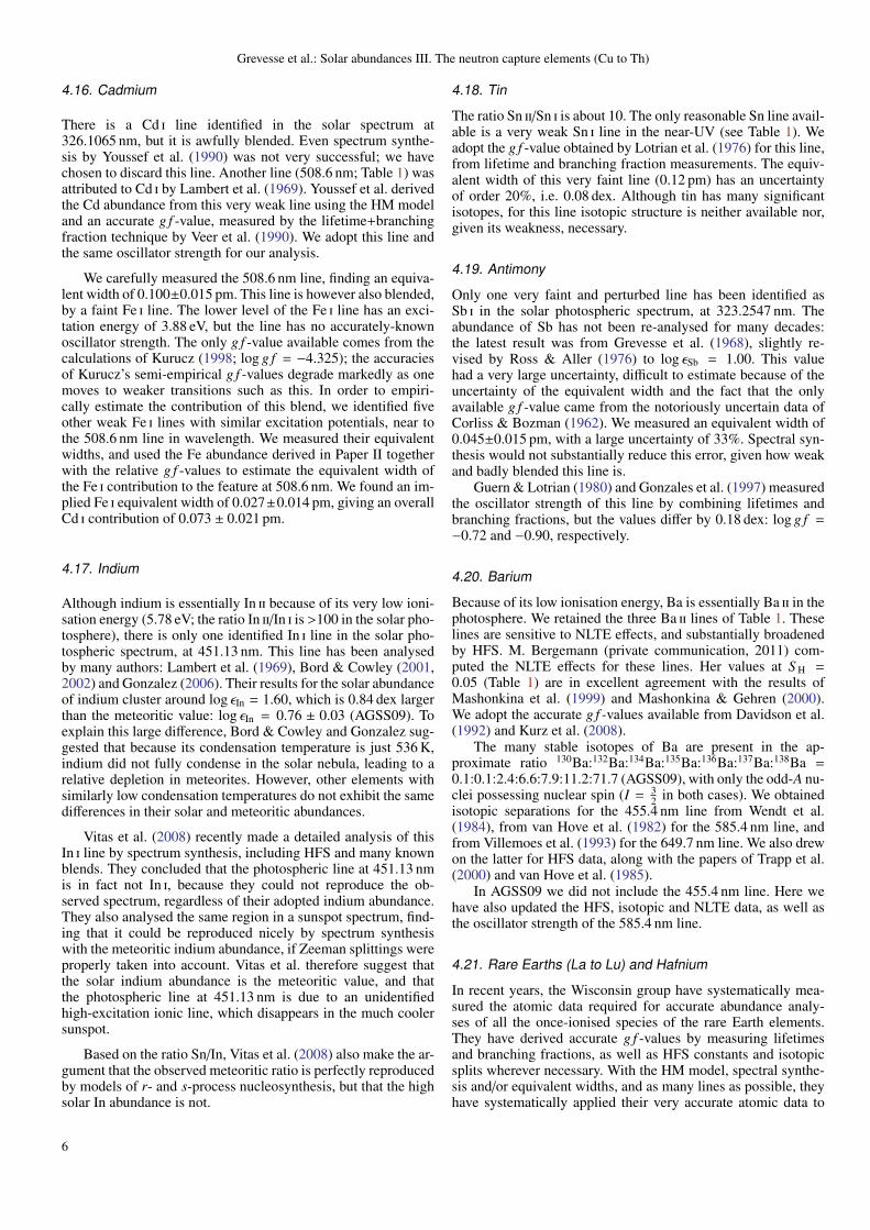
4.16. Cadmium
There is a Cd i line identified in the solar spectrum at326.1065 nm, but it is awfully blended. Even spectrum synthe-sis by Youssef et al. (1990) was not very successful; we havechosen to discard this line. Another line (508.6 nm; Table 1) wasattributed to Cd i by Lambert et al. (1969). Youssef et al. derivedthe Cd abundance from this very weak line using the HM modeland an accurate g f -value, measured by the lifetime+branchingfraction technique by Veer et al. (1990). We adopt this line andthe same oscillator strength for our analysis.
We carefully measured the 508.6 nm line, finding an equiva-lent width of 0.100±0.015 pm. This line is however also blended,by a faint Fe i line. The lower level of the Fe i line has an exci-tation energy of 3.88 eV, but the line has no accurately-knownoscillator strength. The only g f -value available comes from thecalculations of Kurucz (1998; log g f = −4.325); the accuraciesof Kurucz’s semi-empirical g f -values degrade markedly as onemoves to weaker transitions such as this. In order to empiri-cally estimate the contribution of this blend, we identified fiveother weak Fe i lines with similar excitation potentials, near tothe 508.6 nm line in wavelength. We measured their equivalentwidths, and used the Fe abundance derived in Paper II togetherwith the relative g f -values to estimate the equivalent width ofthe Fe i contribution to the feature at 508.6 nm. We found an im-plied Fe i equivalent width of 0.027±0.014 pm, giving an overallCd i contribution of 0.073 ± 0.021 pm.
4.17. Indium
Although indium is essentially In ii because of its very low ioni-sation energy (5.78 eV; the ratio In ii/In i is >100 in the solar pho-tosphere), there is only one identified In i line in the solar pho-tospheric spectrum, at 451.13 nm. This line has been analysedby many authors: Lambert et al. (1969), Bord & Cowley (2001,2002) and Gonzalez (2006). Their results for the solar abundanceof indium cluster around log εIn = 1.60, which is 0.84 dex largerthan the meteoritic value: log εIn = 0.76 ± 0.03 (AGSS09). Toexplain this large difference, Bord & Cowley and Gonzalez sug-gested that because its condensation temperature is just 536 K,indium did not fully condense in the solar nebula, leading to arelative depletion in meteorites. However, other elements withsimilarly low condensation temperatures do not exhibit the samedifferences in their solar and meteoritic abundances.
Vitas et al. (2008) recently made a detailed analysis of thisIn i line by spectrum synthesis, including HFS and many knownblends. They concluded that the photospheric line at 451.13 nmis in fact not In i, because they could not reproduce the ob-served spectrum, regardless of their adopted indium abundance.They also analysed the same region in a sunspot spectrum, find-ing that it could be reproduced nicely by spectrum synthesiswith the meteoritic indium abundance, if Zeeman splittings wereproperly taken into account. Vitas et al. therefore suggest thatthe solar indium abundance is the meteoritic value, and thatthe photospheric line at 451.13 nm is due to an unidentifiedhigh-excitation ionic line, which disappears in the much coolersunspot.
Based on the ratio Sn/In, Vitas et al. (2008) also make the ar-gument that the observed meteoritic ratio is perfectly reproducedby models of r- and s-process nucleosynthesis, but that the highsolar In abundance is not.
4.18. Tin
The ratio Sn ii/Sn i is about 10. The only reasonable Sn line avail-able is a very weak Sn i line in the near-UV (see Table 1). Weadopt the g f -value obtained by Lotrian et al. (1976) for this line,from lifetime and branching fraction measurements. The equiv-alent width of this very faint line (0.12 pm) has an uncertaintyof order 20%, i.e. 0.08 dex. Although tin has many significantisotopes, for this line isotopic structure is neither available nor,given its weakness, necessary.
4.19. Antimony
Only one very faint and perturbed line has been identified asSb i in the solar photospheric spectrum, at 323.2547 nm. Theabundance of Sb has not been re-analysed for many decades:the latest result was from Grevesse et al. (1968), slightly re-vised by Ross & Aller (1976) to log εSb = 1.00. This valuehad a very large uncertainty, difficult to estimate because of theuncertainty of the equivalent width and the fact that the onlyavailable g f -value came from the notoriously uncertain data ofCorliss & Bozman (1962). We measured an equivalent width of0.045±0.015 pm, with a large uncertainty of 33%. Spectral syn-thesis would not substantially reduce this error, given how weakand badly blended this line is.
Guern & Lotrian (1980) and Gonzales et al. (1997) measuredthe oscillator strength of this line by combining lifetimes andbranching fractions, but the values differ by 0.18 dex: log g f =−0.72 and −0.90, respectively.
4.20. Barium
Because of its low ionisation energy, Ba is essentially Ba ii in thephotosphere. We retained the three Ba ii lines of Table 1. Theselines are sensitive to NLTE effects, and substantially broadenedby HFS. M. Bergemann (private communication, 2011) com-puted the NLTE effects for these lines. Her values at S H =0.05 (Table 1) are in excellent agreement with the results ofMashonkina et al. (1999) and Mashonkina & Gehren (2000).We adopt the accurate g f -values available from Davidson et al.(1992) and Kurz et al. (2008).
The many stable isotopes of Ba are present in the ap-proximate ratio 130Ba:132Ba:134Ba:135Ba:136Ba:137Ba:138Ba =0.1:0.1:2.4:6.6:7.9:11.2:71.7 (AGSS09), with only the odd-A nu-clei possessing nuclear spin (I = 3
2 in both cases). We obtainedisotopic separations for the 455.4 nm line from Wendt et al.(1984), from van Hove et al. (1982) for the 585.4 nm line, andfrom Villemoes et al. (1993) for the 649.7 nm line. We also drewon the latter for HFS data, along with the papers of Trapp et al.(2000) and van Hove et al. (1985).
In AGSS09 we did not include the 455.4 nm line. Here wehave also updated the HFS, isotopic and NLTE data, as well asthe oscillator strength of the 585.4 nm line.
4.21. Rare Earths (La to Lu) and Hafnium
In recent years, the Wisconsin group have systematically mea-sured the atomic data required for accurate abundance analy-ses of all the once-ionised species of the rare Earth elements.They have derived accurate g f -values by measuring lifetimesand branching fractions, as well as HFS constants and isotopicsplits wherever necessary. With the HM model, spectral synthe-sis and/or equivalent widths, and as many lines as possible, theyhave systematically applied their very accurate atomic data to
6
Grevesse et al.: Solar abundances III. The neutron capture elements (Cu to Th)
the determination of the solar abundances of all the rare Earthelements (La: Lawler et al. 2001a, Ce: Lawler et al. 2009, Nd:Den Hartog et al. 2003, Sm: Lawler et al. 2006, Eu: Lawler et al.2001b, Gd: Den Hartog et al. 2006, Tb: Lawler et al. 2001c, Ho:Lawler et al. 2004, Er: Lawler et al. 2008), Pr, Dy, Tm, Yb andLu: Sneden et al. 2009), as well as Hf (Lawler et al. 2007).
We have not repeated the careful spectral synthesis computa-tions done by Sneden, Lawler and collaborators, but rather cor-rected them for the abundance differences we see between theresults with our 3D model and the HM model. For this purposewe have selected a sample of representative lines of each species,and have derived the 3D−HM abundance differences. We in-cluded all HFS and isotopic splittings summarised by Snedenet al. (2009) in our calculations.
For Nd, new g f -values are also available from Li et al.(2007). Taking the mean of g f -values from Li et al. (2007) andfrom Den Hartog et al. (2003) produces exactly the same abun-dance as using only the values of Den Hartog et al, however.
For Sm ii, new accurate g f -values have been measured byRehse et al. (2006), which agree quite well with the values ofLawler et al. (2006). We chose to adopt the mean of the g f -values from these two sources. In AGSS09 we simply adoptedthe values of Lawler et al. (2006).
As in the analysis of AGSS09, for Eu we also applied asmall NLTE correction of +0.03 dex for every line, as derivedby Mashonkina & Gehren (2000). We are not aware of any otherNLTE study of rare Earth elements in the Sun.
For Tb ii, we only kept one of the three lines (365.9 nm) usedby Lawler et al. (2001c), because of the difficulty in fitting theprofiles of the other two, due to blends and very wide HFS.
4.22. Tungsten
The ratio W ii/W i is of order ten in the solar photosphere butunfortunately no W ii lines are available in the solar spectrum.Holweger & Werner (1982) used spectral synthesis to analysethe two weak W i lines at 400.9 and 484.4 nm with the HMmodel. New g f -values have become available from den Hartoget al. (1987) for both lines, and from Kling & Koch (1999) forthe 484.4 nm line. Here we update the results of Holweger &Werner for the new g f -values (where we take the mean of thetwo new values for the 484.4 nm line); we did not previouslyapply this update in AGSS09.
The lines are too faint for isotopic or hyperfine structure tomatter. This is in fact true of all lines we use from elements heav-ier than Hf, so we will discuss neither HFS nor isotopic effectsany further in this Section.
4.23. Osmium
Only very few faint lines of Os i have been identified in thesolar spectrum. Kwiatkowsky et al. (1984) measured accuratelifetimes and used branching fractions from Corliss & Bozman(1962) to derive g f -values for a few Os i lines of solar inter-est. Quinet et al. (2006) recently made new measurements oflifetimes and combined them with modern theoretical branch-ing fractions, leading to values in good agreement with those ofKwiatkowsky et al. (1984).
Kwiatkowsky et al. (1984) used a series of nine Os i lines toderive the solar abundance. Quinet et al. (2006) however showedthat many of these lines are too faint and blended to be reliablymeasured. We agree with Quinet et al. (2006) that very few Os ilines are realistically usable (see their Table 7). We are ultimately
even more demanding than them in our line selection: we onlyretain the 330.2 nm line as the unique tracer of the solar Os abun-dance. We adopt the accurate experimental oscillator strength ofIvarsson et al. (2003) for this line, but note that the value dif-fers from that of Quinet et al. (2006) by only 0.003 dex. The twoother lines considered by Quinet et al. (327.0 and 442.0 nm; seetheir figure 6), are very difficult to analyse accurately, even byspectral synthesis.
4.24. Iridium
Drake & Aller (1976) analysed the Ir i line at 322.1 nm by spec-trum synthesis. Youssef & Khalil (1988) analysed three Ir i linesin the near-UV, including the 322.1 nm line, also by spectrumsynthesis using the HM model.
We retain only the 322.1 nm Ir i line, as the other two usedby Youssef & Khalil (1988) are too heavily perturbed. Even the322.1 nm line is itself heavily blended. Rechecking this line inthe Jungfraujoch solar tracing (Delbouille et al. 1973; no trac-ing is available from Kitt Peak at these wavelengths) we noticedthat Youssef & Khalil’s adopted continuum was too high in thisspectral region. We therefore directly remeasured the equivalentwidth of this blended line: 0.975±0.125 pm. We confirmed thisvalue using spectral synthesis with the HM solar photosphericmodel.
We have been able to derive a very accurate g f -value for322.1 nm line, using lifetime measurements by Gough et al.(1983; uncertainty 3.6%) and Xu et al. (2007; uncertainty 6.8%).We weighted these lifetimes by their respective uncertainties andtook the mean, then paired the resulting value with the branchingfraction measured by Gough et al. We did not use the theoreticalbranching fraction of Xu et al. because of its uncertain accuracy.
4.25. Gold
Youssef (1986) used spectral synthesis with the HM model toanalyse the much-perturbed Au i 312.3 nm line (Table 1), theonly useful Au feature in the solar spectrum. We carefully re-measured this Au i line on the Jungfraujoch disc-centre solarspectrum (Delbouille et al. 1973); no Kitt Peak spectrum is avail-able in this wavelength region. We found an equivalent width of0.29 pm, with an uncertainty of 10%.
A very weak Fe i line is known to exist coincident withthe Au i line, with parameters λ = 312.2775 nm, Eexc = 2.45 eV,log g f = −4.144 (Kurucz 1998). Unfortunately, the oscillatorstrength is not reliable enough to make any serious estimate ofthe contribution to the equivalent width of the Au i line, and thespectrum is far too crowded in this region to employ the samestrategy as we did for Cd i, where we relied on a number of othernearby faint Fe i lines.
The best available g f -value for the Au i line comes fromHannaford et al. (1981), who obtained log g f = −0.95 ± 0.06with lifetime and branching fraction measurements. The lifetimeof Hannaford et al. for the upper level agrees perfectly with thatobtained by Gaarde et al. (1994) using a similar technique.
4.26. Lead
Biemont et al. (2000) used one Pb i line, for which they had ac-curately derived the g f -value, to revise the solar Pb abundance.We use the same line and oscillator strength (Table 1), but ourequivalent width is 0.855±0.035 pm instead of 0.91 pm, derivedanew for this paper by both direct measurement and spectrum
7
Grevesse et al.: Solar abundances III. The neutron capture elements (Cu to Th)
synthesis. This line is situated in the outer red wing of an ex-tremely strong line with contributions from Co i, Fe i and V i,and in the outer blue wing of a somewhat less strong Fe i line.The continuum is very difficult to determine in this crowded re-gion, but a viable reference point can be found at 3683.8 Å. Werule out the large equivalent width of Biemont et al.; our spectralsynthesis calculations confirm that their continuum placement isincorrect.
Mashonkina et al. (2012) computed the effect of departuresfrom LTE on the formation of this Pb i line at the centre of thesolar disc, which are substantial. Between S H = 0 and S H = 1,the NLTE correction with the marcs model atmosphere variesfrom +0.15 to +0.07 dex. We adopt Mashonkina et al.’s pre-ferred value of +0.12 dex, derived with S H = 0.1. At the timeof AGSS09, no NLTE correction was available.
4.27. Thorium
The only reliable faint Th ii line lies at 401.9 nm, in the red wingof a much stronger Fe i line. It is also blended by Co i and V ilines, both with about the same wavelengths.
The best oscillator strength for the Th ii line comes fromthe accurate lifetime+branching fraction results of Nilsson etal. (2002). Atomic data (wavelengths, HFS and g f -values) con-cerning the blends are known from the works of Learner et al.(1991), Lawler et al. (1990) and Pickering & Semeniuk (1995).Although the g f -value for the Co i line (log g f = −2.27 ± 0.04,Eexc = 2.28 eV) is very accurate (Lawler et al. 1990), the valuefor the V i blend (Eexc = 1.80 eV) is probably less well known,even though Pickering & Semeniuk give log g f = −1.30 ± 0.04.The stated uncertainty is for the relative value with respect tothe g f -values of two stronger V i lines, to which Pickering &Semeniuk compared this line. The absolute g f -values of thesestronger lines come from from Kurucz (1998), and are onlyknown to about ±0.08 dex.
We measured the total equivalent width of the feature con-taining Th ii. We also computed the contributions of the Co i andV i blends from the g f -values above, and the abundances de-rived in Paper II, employing a number of different solar photo-spheric model atmospheres. The equivalent widths of the twoblends predicted in this way are almost model-independent. Wefound predicted equivalent widths of 0.208 pm for the Co i blend,and 0.038 pm for the V i blend. As the total measured equivalentwidth is 0.56 pm, this leaves 0.314 pm for Th ii. We estimate theuncertainty of the Th ii contribution to be of order 20%, basedon the uncertainty of the total measured equivalent width andthe uncertainties of the Co i and V i contributions.
Mashonkina et al. (2012) estimated small NLTE correctionsof between +0.06 dex (S H = 0) and 0.00 dex (S H = 1) forthis Th ii line, using the marcs model atmosphere. We adopt∆NLTE = +0.01 dex, corresponding to S H = 0.1 (Mashonkinaet al.’s preferred value). This NLTE correction was not availablefor AGSS09.
5. Derived solar elemental abundances
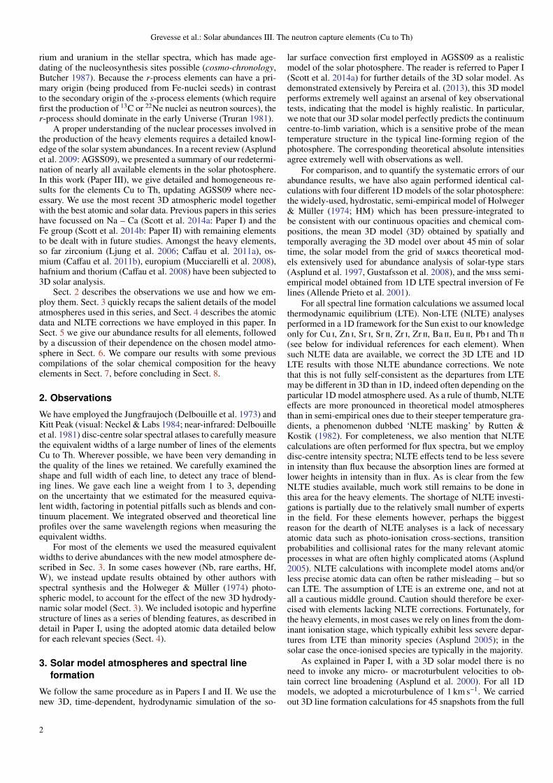
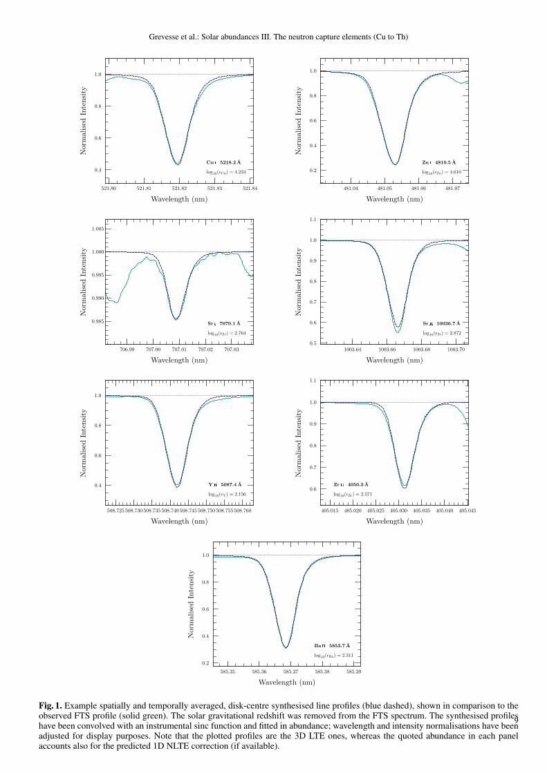
The detailed results for the different model atmospheres we usedare presented in Table 1, with each element individually dis-cussed below. Line profiles produced in 3D generally show verygood agreement with the observed spectrum; some examples aregiven in Fig. 1.
Besides statistical errors in our derived abundances (whichwe specify as the standard deviation of the mean), we quantify
three possible systematic errors arising from potential problemsin the atmospheric and atomic modelling: departures from LTE,the mean photospheric temperature structure and atmosphericinhomogeneities. We add these in quadrature to the statisticalerrors to estimate overall uncertainties. Full details can be foundin Paper I.
Below we often refer to the “3D effect” on the derived ele-mental abundances. We define this 3D effect as log ε3D−log εHM,i.e. the correction to bring the abundance computed with the HMmodel into agreement with the abundance obtained with our 3Dmodel. Although this is not strictly just the effect of using a3D model atmosphere rather than a 1D one (see Sec. 6 for adiscussion), we use this definition because the HM model hasbeen the de facto standard for abundance determinations in pastdecades. We note that other authors prefer to define the 3D ef-fect as log ε3D − log ε〈3D〉 to isolate the impact of the atmosphericinhomogeneities. We argue however that differences in the meanstratification arising from the treatment of convection should beconsidered when evaluating the full impact of using 3D modelsrather than 1D ones.
5.1. Copper
Our 3D+NLTE copper abundance is
log εCu = 4.18 ± 0.05 (±0.02 stat, ±0.04 sys).
The 3D effect on these lines is rather small; with the HM modelthe abundance is 4.21. Interestingly, accounting for departuresfrom LTE as computed by Shi et al. (2014) slightly increasesthe line-to-line scatter (σ = 0.03 and 0.05 dex, respectively) butthe net effect on the Cu abundance is small (−0.01 dex). Our Cuabundances in 3D and with HM are not too different from theresults of Shi et al. (2014; 4.19 ± 0.10, from ten lines), Kock &Richter (1968; 4.16±0.08, from six lines) and Sneden & Crocker(1988; 4.12, from two lines). We do not reproduce the ratherlarge difference in abundance found by Shi et al. (2014) betweenthe low and high excitation lines with the HM model. However,our sample only includes one of the low excitation lines usedby those authors. Our adopted value agrees reasonably well withthe meteoritic abundance (log εCu = 4.25 ± 0.04; AGSS09).
5.2. Zinc
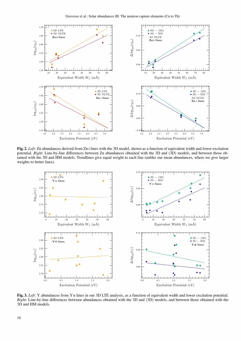
Our 3D+NLTE zinc abundance is
log εZn = 4.56 ± 0.05 (±0.03 stat, ±0.04 sys).
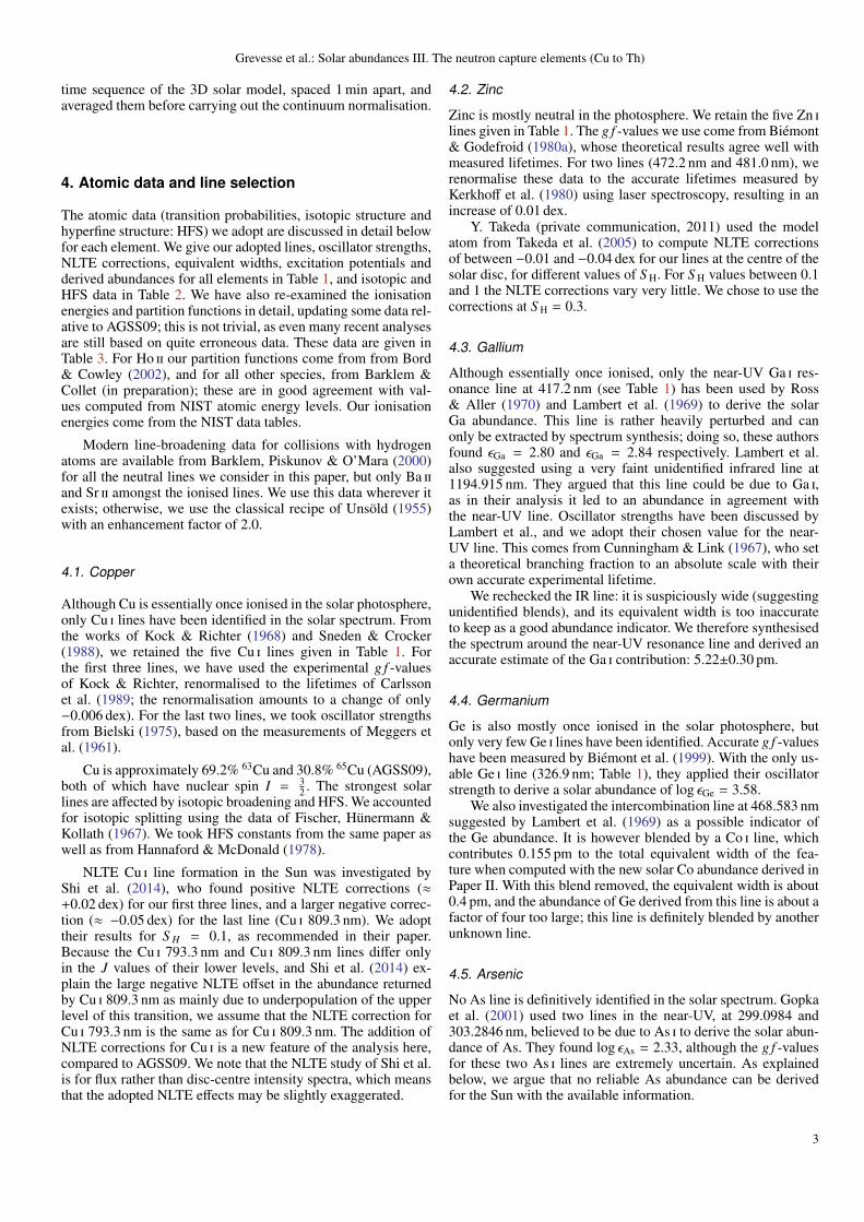
We note that the abundance only varies by 0.026 dex when wego from SH=0.1 to 1. The mean NLTE correction is also verysmall: −0.02 dex. Zn i is one of the few species where the HMmodel gives a slightly lower abundance than the 3D model:log εZn = 4.53. Referring to Fig. 2, we see that this is essen-tially due to two strong lines only, indicating that the micro-turbulence adopted in 1D is probably too high, or possibly thatDoppler broadening due to convection is insufficient in the 3Dcase. Curiously, these two lines return an abundance approxi-mately 0.1 dex larger with the 3D model than any 1D model, in-cluding 〈3D〉. This leads to pronounced trends with line strengthand excitation potential, although the significance of the trendsis debatable given the small number of lines. These are preciselythe two lines for which we renormalised oscillator strengths tothe scale of Kerkhoff et al. (1980), but this operation amountsto a change of just 0.01 dex, so cannot explain the 0.1 dex off-set. Another possibility is that the NLTE corrections may have
8
Grevesse et al.: Solar abundances III. The neutron capture elements (Cu to Th)
521.80 521.81 521.82 521.83 521.84
Wavelength (nm)
0.4
0.6
0.8
1.0
NormalisedIntensity
Cu i 5218.2 A
log10(εCu) = 4.234
706.99 707.00 707.01 707.02 707.03
Wavelength (nm)
0.985
0.990
0.995
1.000
1.005
NormalisedIntensity
Sr i 7070.1 A
log10(εSr) = 2.764
508.725 508.730 508.735 508.740 508.745 508.750 508.755 508.760
Wavelength (nm)
0.4
0.6
0.8
1.0
Norm
alised
Intensity
Y ii 5087.4 A
log10(εY) = 2.156
481.04 481.05 481.06 481.07
Wavelength (nm)
0.2
0.4
0.6
0.8
1.0
NormalisedIntensity
Zn i 4810.5 A
log10(εZn) = 4.610
1003.64 1003.66 1003.68 1003.70
Wavelength (nm)
0.5
0.6
0.7
0.8
0.9
1.0
1.1
NormalisedIntensity
Sr ii 10036.7 A
log10(εSr) = 2.872
405.015 405.020 405.025 405.030 405.035 405.040 405.045
Wavelength (nm)
0.6
0.7
0.8
0.9
1.0
1.1
Normalised
Intensity
Zr ii 4050.3 A
log10(εZr) = 2.571
585.35 585.36 585.37 585.38 585.39
Wavelength (nm)
0.2
0.4
0.6
0.8
1.0
NormalisedIntensity
Ba ii 5853.7 A
log10(εBa) = 2.311
Fig. 1. Example spatially and temporally averaged, disk-centre synthesised line profiles (blue dashed), shown in comparison to theobserved FTS profile (solid green). The solar gravitational redshift was removed from the FTS spectrum. The synthesised profileshave been convolved with an instrumental sinc function and fitted in abundance; wavelength and intensity normalisations have beenadjusted for display purposes. Note that the plotted profiles are the 3D LTE ones, whereas the quoted abundance in each panelaccounts also for the predicted 1D NLTE correction (if available).
9
Grevesse et al.: Solar abundances III. The neutron capture elements (Cu to Th)
★
★
★
★
★
●
●
●
●
●
★●
10 20 30 40 50 60 70 80
Equivalent Width Wλ (mA)
4.45
4.50
4.55
4.60
4.65
4.70
log10(ε
Zn)
3D LTE3D NLTE
Zn i lines
★
★
★
★
★
●
●
●
●
●
★●
3.5 4.0 4.5 5.0 5.5 6.0 6.5 7.0
Excitation Potential (eV)
4.45
4.50
4.55
4.60
4.65
4.70
log10(ε
Zn)
3D LTE3D NLTE
Zn i lines
★ ★
★★
★
●●
●
●
●
★●
10 20 30 40 50 60 70 80
Equivalent Width Wλ (mA)
0.00
0.05
0.10
∆lo
g10(ε
Zn)
3D − 〈3D〉3D − HM
All NLTEZn i lines
★★
★★
★
●●
●●
●
★●
3.5 4.0 4.5 5.0 5.5 6.0 6.5 7.0
Excitation Potential (eV)
−0.05
0.00
0.05
0.10
∆lo
g10(ε
Zn)
3D − 〈3D〉3D − HM
All NLTEZn i lines
Fig. 2. Left: Zn abundances derived from Zn i lines with the 3D model, shown as a function of equivalent width and lower excitationpotential. Right: Line-by-line differences between Zn abundances obtained with the 3D and 〈3D〉 models, and between those ob-tained with the 3D and HM models. Trendlines give equal weight to each line (unlike our mean abundances, where we give largerweights to better lines).
★
★
★
★
★
★
★
★
★
★
0 10 20 30 40 50 60
Equivalent Width Wλ (mA)
2.10
2.15
2.20
2.25
2.30
log10(ε
Y)
3D LTE
Y ii lines
★
★
★
★
★
★
★
★
★
★
0.0 0.5 1.0 1.5 2.0
Excitation Potential (eV)
2.10
2.15
2.20
2.25
2.30
log10(ε
Y)
3D LTE
Y ii lines
★
★
★
★
★
★
★ ★★
●
●
●
●
●
●
●
●●
★●
0 10 20 30 40 50 60
Equivalent Width Wλ (mA)
0.00
0.05
0.10
∆lo
g10(ε
Y)
3D − 〈3D〉3D − HM
Y ii lines
★
★
★
★
★
★
★ ★ ★
●
●
●
●
●
●
●
● ●
★●
0.0 0.5 1.0 1.5 2.0
Excitation Potential (eV)
0.00
0.05
0.10
∆lo
g10(ε
Y)
3D − 〈3D〉3D − HM
Y ii lines
Fig. 3. Left: Y abundances from Y ii lines in our 3D LTE analysis, as a function of equivalent width and lower excitation potential.Right: Line-by-line differences between abundances obtained with the 3D and 〈3D〉 models, and between those obtained with the3D and HM models.
10
Grevesse et al.: Solar abundances III. The neutron capture elements (Cu to Th)
★
★
★
★
★
★
★
★
★
★
★
10 20 30 40 50 60
Equivalent Width Wλ (mA)
2.50
2.55
2.60
2.65lo
g10(ε
Zr)
3D LTE
Zr ii lines
★
★★
★★★
★
★
★★
●
●●
●
●●
●
●
●●
★●
10 20 30 40 50 60
Equivalent Width Wλ (mA)
−0.05
0.00
0.05
0.10
0.15
∆lo
g10(ε
Zr)
3D − 〈3D〉3D − HM
Zr ii lines
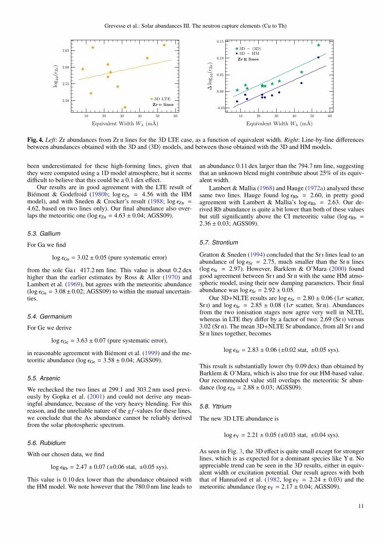
Fig. 4. Left: Zr abundances from Zr ii lines for the 3D LTE case, as a function of equivalent width. Right: Line-by-line differencesbetween abundances obtained with the 3D and 〈3D〉 models, and between those obtained with the 3D and HM models.
been underestimated for these high-forming lines, given thatthey were computed using a 1D model atmosphere, but it seemsdifficult to believe that this could be a 0.1 dex effect.
Our results are in good agreement with the LTE result ofBiemont & Godefroid (1980b; log εZn = 4.56 with the HMmodel), and with Sneden & Crocker’s result (1988; log εZn =4.62, based on two lines only). Our final abundance also over-laps the meteoritic one (log εZn = 4.63 ± 0.04; AGSS09).
5.3. Gallium
For Ga we find
log εGa = 3.02 ± 0.05 (pure systematic error)
from the sole Ga i 417.2 nm line. This value is about 0.2 dexhigher than the earlier estimates by Ross & Aller (1970) andLambert et al. (1969), but agrees with the meteoritic abundance(log εGa = 3.08± 0.02; AGSS09) to within the mutual uncertain-ties.
5.4. Germanium
For Ge we derive
log εGe = 3.63 ± 0.07 (pure systematic error),
in reasonable agreement with Biemont et al. (1999) and the me-teoritic abundance (log εGe = 3.58 ± 0.04; AGSS09).
5.5. Arsenic
We rechecked the two lines at 299.1 and 303.2 nm used previ-ously by Gopka et al. (2001) and could not derive any mean-ingful abundance, because of the very heavy blending. For thisreason, and the unreliable nature of the g f -values for these lines,we conclude that the As abundance cannot be reliably derivedfrom the solar photospheric spectrum.
5.6. Rubidium
With our chosen data, we find
log εRb = 2.47 ± 0.07 (±0.06 stat, ±0.05 sys).
This value is 0.10 dex lower than the abundance obtained withthe HM model. We note however that the 780.0 nm line leads to
an abundance 0.11 dex larger than the 794.7 nm line, suggestingthat an unknown blend might contribute about 25% of its equiv-alent width.
Lambert & Mallia (1968) and Hauge (1972a) analysed thesesame two lines. Hauge found log εRb = 2.60, in pretty goodagreement with Lambert & Mallia’s log εRb = 2.63. Our de-rived Rb abundance is quite a bit lower than both of these valuesbut still significantly above the CI meteoritic value (log εRb =2.36 ± 0.03; AGSS09).
5.7. Strontium
Gratton & Sneden (1994) concluded that the Sr i lines lead to anabundance of log εSr = 2.75, much smaller than the Sr ii lines(log εSr = 2.97). However, Barklem & O’Mara (2000) foundgood agreement between Sr i and Sr ii with the same HM atmo-spheric model, using their new damping parameters. Their finalabundance was log εSr = 2.92 ± 0.05.
Our 3D+NLTE results are log εSr = 2.80 ± 0.06 (1σ scatter,Sr i) and log εSr = 2.85 ± 0.08 (1σ scatter, Sr ii). Abundancesfrom the two ionisation stages now agree very well in NLTE,whereas in LTE they differ by a factor of two: 2.69 (Sr i) versus3.02 (Sr ii). The mean 3D+NLTE Sr abundance, from all Sr i andSr ii lines together, becomes
log εSr = 2.83 ± 0.06 (±0.02 stat, ±0.05 sys).
This result is substantially lower (by 0.09 dex) than obtained byBarklem & O’Mara, which is also true for our HM-based value.Our recommended value still overlaps the meteoritic Sr abun-dance (log εZn = 2.88 ± 0.03; AGSS09).
5.8. Yttrium
The new 3D LTE abundance is
log εY = 2.21 ± 0.05 (±0.03 stat, ±0.04 sys).
As seen in Fig. 3, the 3D effect is quite small except for strongerlines, which is as expected for a dominant species like Y ii. Noappreciable trend can be seen in the 3D results, either in equiv-alent width or excitation potential. Our result agrees with boththat of Hannaford et al. (1982, log εY = 2.24 ± 0.03) and themeteoritic abundance (log εY = 2.17 ± 0.04; AGSS09).
11
Grevesse et al.: Solar abundances III. The neutron capture elements (Cu to Th)
★
★
★
★
★
★★
0 5 10 15 20
Equivalent Width Wλ (mA)
1.6
1.7
1.8
1.9
log10(ε
Ru)
3D LTE
Ru i lines★
★
★★★★
●
●
●
●●
●
★●
0 5 10 15 20
Equivalent Width Wλ (mA)
−0.15
−0.10
−0.05
∆lo
g10(ε
Ru)
3D − 〈3D〉3D − HM
Ru i lines
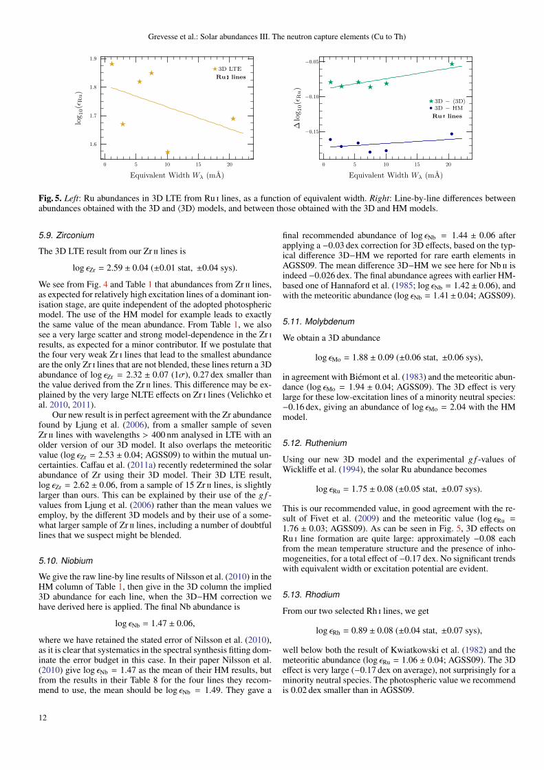
Fig. 5. Left: Ru abundances in 3D LTE from Ru i lines, as a function of equivalent width. Right: Line-by-line differences betweenabundances obtained with the 3D and 〈3D〉 models, and between those obtained with the 3D and HM models.
5.9. Zirconium
The 3D LTE result from our Zr ii lines is
log εZr = 2.59 ± 0.04 (±0.01 stat, ±0.04 sys).
We see from Fig. 4 and Table 1 that abundances from Zr ii lines,as expected for relatively high excitation lines of a dominant ion-isation stage, are quite independent of the adopted photosphericmodel. The use of the HM model for example leads to exactlythe same value of the mean abundance. From Table 1, we alsosee a very large scatter and strong model-dependence in the Zr iresults, as expected for a minor contributor. If we postulate thatthe four very weak Zr i lines that lead to the smallest abundanceare the only Zr i lines that are not blended, these lines return a 3Dabundance of log εZr = 2.32 ± 0.07 (1σ), 0.27 dex smaller thanthe value derived from the Zr ii lines. This difference may be ex-plained by the very large NLTE effects on Zr i lines (Velichko etal. 2010, 2011).
Our new result is in perfect agreement with the Zr abundancefound by Ljung et al. (2006), from a smaller sample of sevenZr ii lines with wavelengths > 400 nm analysed in LTE with anolder version of our 3D model. It also overlaps the meteoriticvalue (log εZr = 2.53 ± 0.04; AGSS09) to within the mutual un-certainties. Caffau et al. (2011a) recently redetermined the solarabundance of Zr using their 3D model. Their 3D LTE result,log εZr = 2.62 ± 0.06, from a sample of 15 Zr ii lines, is slightlylarger than ours. This can be explained by their use of the g f -values from Ljung et al. (2006) rather than the mean values weemploy, by the different 3D models and by their use of a some-what larger sample of Zr ii lines, including a number of doubtfullines that we suspect might be blended.
5.10. Niobium
We give the raw line-by line results of Nilsson et al. (2010) in theHM column of Table 1, then give in the 3D column the implied3D abundance for each line, when the 3D−HM correction wehave derived here is applied. The final Nb abundance is
log εNb = 1.47 ± 0.06,
where we have retained the stated error of Nilsson et al. (2010),as it is clear that systematics in the spectral synthesis fitting dom-inate the error budget in this case. In their paper Nilsson et al.(2010) give log εNb = 1.47 as the mean of their HM results, butfrom the results in their Table 8 for the four lines they recom-mend to use, the mean should be log εNb = 1.49. They gave a
final recommended abundance of log εNb = 1.44 ± 0.06 afterapplying a −0.03 dex correction for 3D effects, based on the typ-ical difference 3D−HM we reported for rare earth elements inAGSS09. The mean difference 3D−HM we see here for Nb ii isindeed −0.026 dex. The final abundance agrees with earlier HM-based one of Hannaford et al. (1985; log εNb = 1.42 ± 0.06), andwith the meteoritic abundance (log εNb = 1.41± 0.04; AGSS09).
5.11. Molybdenum
We obtain a 3D abundance
log εMo = 1.88 ± 0.09 (±0.06 stat, ±0.06 sys),
in agreement with Biemont et al. (1983) and the meteoritic abun-dance (log εMo = 1.94 ± 0.04; AGSS09). The 3D effect is verylarge for these low-excitation lines of a minority neutral species:−0.16 dex, giving an abundance of log εMo = 2.04 with the HMmodel.
5.12. Ruthenium
Using our new 3D model and the experimental g f -values ofWickliffe et al. (1994), the solar Ru abundance becomes
log εRu = 1.75 ± 0.08 (±0.05 stat, ±0.07 sys).
This is our recommended value, in good agreement with the re-sult of Fivet et al. (2009) and the meteoritic value (log εRu =1.76 ± 0.03; AGSS09). As can be seen in Fig. 5, 3D effects onRu i line formation are quite large: approximately −0.08 eachfrom the mean temperature structure and the presence of inho-mogeneities, for a total effect of −0.17 dex. No significant trendswith equivalent width or excitation potential are evident.
5.13. Rhodium
From our two selected Rh i lines, we get
log εRh = 0.89 ± 0.08 (±0.04 stat, ±0.07 sys),
well below both the result of Kwiatkowski et al. (1982) and themeteoritic abundance (log εRu = 1.06 ± 0.04; AGSS09). The 3Deffect is very large (−0.17 dex on average), not surprisingly for aminority neutral species. The photospheric value we recommendis 0.02 dex smaller than in AGSS09.
12
Grevesse et al.: Solar abundances III. The neutron capture elements (Cu to Th)
5.14. Palladium
Our 3D LTE result for Pd is
log εPd = 1.55 ± 0.06 (±0.02 stat, ±0.06 sys).
The 3D effect, −0.06 dex, is smaller than for the other minor-ity species Rb, Zr, Mo, Ru and Rh, as the ratio ion/neutral issmaller for Pd. The Pd abundance derived with the HM model islog εPd = 1.61, somewhat lower than found by Xu et al. (2006;log εPd = 1.66 ± 0.04), due in part to our more stringent lineselection. Interestingly, our 3D abundance is substantially lowerthan the meteoritic one (log εPd = 1.65 ± 0.02; AGSS09).
5.15. Silver
Our 3D LTE solar abundance of silver is
log εAg = 0.96 ± 0.10 (±0.09 stat, ±0.06 sys),
in agreement with the earlier value from Grevesse (1984;log εAg = 0.94 ± 0.25), but well below the meteoritic abundance(log εAg = 1.20 ± 0.02; AGSS09). The HM-based abundance issignificantly larger (1.04), but the presence of atmospheric inho-mogeneities, as opposed to the mean stratification, matters little.
5.16. Cadmium
Taking into account the large uncertainty on the measured equiv-alent width (Wλ = 0.073 ± 0.021 pm) of the one Cd i line avail-able, our 3D solar Cd abundance is
log εCd = 1.77 ± 0.15 (pure systematic error).
The 3D effect is small: −0.03 dex. Our result is coincidentallyin perfect agreement with that of Youssef et al. (1990; log εCd =1.77 ± 0.11), and also easily overlaps the meteoritic abundance(log εCd = 1.71 ± 0.03; AGSS09).
5.17. Indium
We adopt the solar abundance of In suggested by Vitas et al.(2008):
log εIn = 0.80 ± 0.20.
Using the meteoritic abundance, the equivalent width ofthe In i contribution to the observed photospheric feature at451.13 nm should be 0.055 pm, i.e. In i contributes < 20% ofthe observed faint photospheric line, which has Wλ = 0.33 pm.In principle, the problems in the photosphere might be relatedto potentially large NLTE and/or 3D effects on In i line forma-tion. If we assume (purely for the sake of argument) that theentire line is In i, then we confirm the high abundance valuewith the HM model: log εIn = 1.61. With the 3D model, wewould instead find log εIn = 1.46, meaning that 3D effects areindeed large (−0.14 dex after rounding), but certainly not largeenough to reconcile the abundance with the meteoritic value.Combining NLTE and 3D effects could never successfully ex-plain the 0.8 dex difference between the photospheric and me-teoritic abundances, confirming the conclusion of Vitas et al.(2008) that the photospheric line is severely blended.
5.18. Tin
Taking into account the error on the equivalent width of the sin-gle Sn i line we use (in addition to our standard error budget),the 3D result is
log εSn = 2.02 ± 0.10 (pure systematic error).
With the HM model we obtained log εSn = 2.13, so the 3D ef-fect is rather large: −0.11 dex. A very old solar abundance byGrevesse et al. (1968; log εSn = 1.32) was revised by Lambert etal. (1969) with a new, more accurate g f -value, and then by Ross& Aller (1976), resulting in log εSn = 2.0±0.4. Our result is veryclose to that of Ross & Aller (1976), and is entirely consistentwith the meteoritic abundance (log εSn = 2.07 ± 0.06; AGSS09).
5.19. Antimony
Taking into account the large uncertainties of the equivalentwidth and the experimental g f -values, we find a solar Sb abun-dance of log εSb ≈ 1.5 ± 0.3. For this reason, we do not recom-mend any photospheric abundance of antimony.
5.20. Barium
For the Sun, the few available Ba ii lines have been analysed byHolweger & Muller (1974), Rutten (1978), Gratton & Sneden(1994), Mashonkina et al. (1999) and Mashonkina & Gehren(2000), among others. The most recent estimate of the solarabundance is log εBa = 2.21 (Mashonkina & Gehren 2000).
We find a 3D+NLTE Ba abundance of
log εBa = 2.25 ± 0.07 (±0.03 stat, ±0.07 sys),
Our HM-based value is actually 0.07 dex lower. The two strongZn i lines are most likely affected by an issue with the adoptedmicroturbulence in 1D or the predicted convective broadeningin the higher layers of the 3D model. Both the HM and 3D re-sults overlap the recommended value of Mashonkina & Gehren(2000), as well as the meteoritic value (log εBa = 2.18 ± 0.03;AGSS09).
5.21. Rare Earths (La to Lu) and Hafnium
As explain in Sect. 4.21, we do not attempt a detailed 3D-basedanalysis of all the often-blended lines of rare Earth elementsand Hf. Instead we rely on the careful work done by Lawler,Sneden and collaborators using 1D spectrum synthesis with theHM model, and simply correct their derived abundance with ourpredicted 3D-HM corrections for a subsample of lines (for eachelement, the lines behave very similarly in this respect so thereis no need to compute the 3D effect for all lines). As expectedfor low excitation lines of a dominant species, the 3D−HM ef-fect on all the rare Earth lines we investigated is small, varyingfrom −0.01 to −0.04 dex. The 3D results for all elements La–Hfare summarised in Table 4.
Updating the original Sm abundance of Lawler et al. for thenew g f -values we describe in Sect. 4.21 leads to a small changein the HM abundance: log εSm = 0.99 instead of 1.00.
Our 3D LTE result for Eu, log εEu = 0.49, is 0.03 dex lowerthan the recent LTE Eu solar abundance found by Mucciarelli etal. (2008; log εEu = 0.52), using their own 3D model. Our recom-mended Eu abundance however also includes NLTE correctionsof +0.03 dex from Mashonkina & Gehren (2000), which cancel
13

Grevesse et al.: Solar abundances III. The neutron capture elements (Cu to Th)
the 3D correction of −0.03 dex to bring our final result into (co-incidentally) perfect agreement with those of both Mucciarelli etal. (2008) and Lawler et al. (2001b).
With the 3D model, the one Tb ii line we retained returnslog εTb = 0.31 ± 0.10. If we had kept all three lines analysed byLawler et al. (2001c), we would have obtained an abundance oflog εTb = 0.24 ± 0.08.
Our new Hf abundance, log εHf = 0.85 ± 0.05, is in verygood agreement with a recent result by Caffau et al. (2008) usingtheir own 3D model: log εHf = 0.87 ± 0.04. Although the solarabundances of all elements from La to Lu are consistent withthe meteoritic values (to within the mutual uncertainties), thesolar abundance of Hf is quite a bit higher than the meteoriticone (log εHf = 0.71 ± 0.02; AGSS09). Perhaps the most naturalexplanation would be erroneous g f -values for the Hf ii lines, butthe experimental data from Lawler et al. (2007) appear reliable.
5.22. Tungsten
Updating the results of Holweger & Werner (1982) for the newg f -values we discuss in Sect. 4.22, the mean abundance be-comes log εW = 1.03. We further updated this result by com-puting the 3D−HM abundance corrections for these two lines:−0.19 dex. This is not surprising for these low excitation lines ofa minor species (W ii/W i ∼ 10). The 3D LTE abundance of Wthus becomes
log εW = 0.83 ± 0.11 (±0.03 stat, ±0.11 sys),
where the systematic error includes both the regular sources(0.08 dex) and the error in the equivalent widths (0.07 dex), dueto the fact that these lines are very weak (0.35 and 0.035 pm re-spectively, cf. Table 1). Even with spectral synthesis these linesare extremely difficult to reproduce accurately. Despite the large3D effects, the solar tungsten abundance is substantially largerthan seen in meteorites (log εW = 0.65± 0.04; AGSS09), similarto the case of Hf mentioned above.
5.23. Osmium
We find with our 3D model an Os abundance of
log εOs = 1.40 ± 0.05 (pure systematic error),
in reasonable agreement with the meteoritic value (log εOs =1.35 ± 0.03; AGSS09). The 3D effect is quite large: −0.09 dex.
An example of the problem with the Os i lines used in pastanalyses is seen in the results of Kwiatkowsky et al. (1984): thedispersion is very large (σ = 0.15 dex), and the difference be-tween the lowest and largest abundances is 0.42 dex. Recent re-sults by Caffau et al. (2011b), who used the lines and solar dataof Kwiatkowsky et al. with their own 3D model, show a similarlyunacceptable dispersion. Their result, log εOs = 1.36 ± 0.19 dex,includes a striking difference of 0.71 dex between the lowestand largest abundance. We note that Caffau et al. used an ob-solete value for the ionisation potential of Os i (8.7 eV), whereasthe correct value is 8.4382 ± 0.0002 eV (Colarusso et al. 1997).We estimate that their abundance results from Os i lines shouldtherefore be increased by about 0.15 dex, to log εOs = 1.51 ±0.19 dex. This result is much larger than what we find here, asexpected from the severely blended nature of some of their cho-sen lines.
5.24. Iridium
With our adopted equivalent width and g f -value, we find a 3Dabundance of
log εIr = 1.42 ± 0.07 (pure systematic error),
where the error includes the uncertainty in the measured equiv-alent width (0.06 dex) and the combined contributions of theusual three systematics (0.04 dex). This abundance is in ratherpoor agreement with the meteoritic value (log εIr = 1.32 ± 0.02;AGSS09). Our result is however consistent with previous deter-minations: Youssef & Khalil (1988) found log εIr = 1.38 ± 0.05,and the result of Drake & Aller (1976) goes from log εIr = 0.82to log εIr = 1.37 when updated to the g f -value we adopt.
5.25. Gold
We find a 3D solar gold abundance of
log εAu = 0.91 ± 0.08 (pure systematic error),
where we have incorporated the uncertainty in the equivalentwidth and g f -value into the final uncertainty. The 3D effectis small: −0.02 dex. Updating the HM spectrum synthesis re-sult of Youssef (1986; log εAu = 0.95) with the 3D−HM ef-fect would lead to log εAu=0.93, in excellent agreement with thevalue we obtain here. Our adopted gold abundance remains sub-stantially higher than the meteoritic value (log εAu = 0.80±0.04;AGSS09).
5.26. Lead
The LTE abundances of lead with the 3D and HM models arelog εPb = 1.80 and 1.93, respectively; the 3D−HM effect is ratherlarge, −0.14 dex after rounding. This is expected because Pb i isa minority species compared to Pb ii in the solar photosphere.
Taking into account the significant NLTE correction(+0.12 dex) of Mashonkina et al. (2012), our final 3D abundanceof Pb becomes
log εPb = 1.92 ± 0.08 (pure systematic error).
This is somewhat smaller than obtained by Biemont et al. (2000;log εPb = 2.00 ± 0.06) with the HM model and an erroneouslylarge equivalent width. Our photospheric Pb abundance is alsosubstantially smaller than the corresponding CI meteoritic value(log εPb = 2.04 ± 0.03; AGSS09).
5.27. Thorium
The 3D+NLTE solar abundance of Th is
log εTh = 0.03 ± 0.10 (pure systematic error),
where the error budget is dominated by the uncertainty in ouradopted equivalent width. Given the overall uncertainty, the pho-tospheric abundance of Th is consistent with the meteoritic value(log εTh = 0.06±0.03; AGSS09). With the HM model, the abun-dance would be log εTh = 0.07.
Our 3D LTE abundance is 15% smaller than the correspond-ing LTE result of Caffau et al. (2008), who found log εTh = 0.08±0.03 with their 3D model. The 0.06 dex difference with our LTEresult can be explained by our improved, model-independent es-timation of the contributions of the blends by Co i and V i. In ouropinion the stated uncertainty of Caffau et al. underestimates theuncertainty of the total contribution of Th ii to the overall equiv-alent width.
14
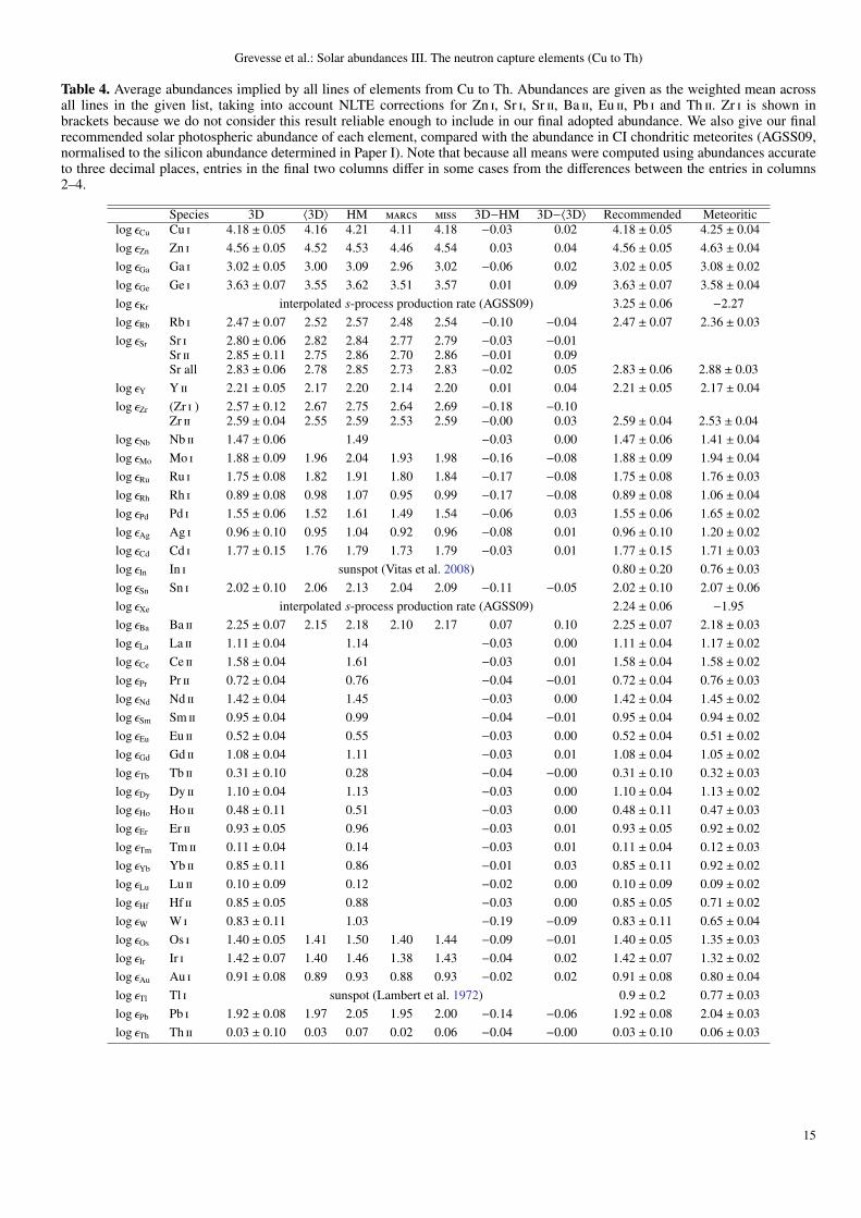
Grevesse et al.: Solar abundances III. The neutron capture elements (Cu to Th)
Table 4. Average abundances implied by all lines of elements from Cu to Th. Abundances are given as the weighted mean acrossall lines in the given list, taking into account NLTE corrections for Zn i, Sr i, Sr ii, Ba ii, Eu ii, Pb i and Th ii. Zr i is shown inbrackets because we do not consider this result reliable enough to include in our final adopted abundance. We also give our finalrecommended solar photospheric abundance of each element, compared with the abundance in CI chondritic meteorites (AGSS09,normalised to the silicon abundance determined in Paper I). Note that because all means were computed using abundances accurateto three decimal places, entries in the final two columns differ in some cases from the differences between the entries in columns2–4.
Species 3D 〈3D〉 HM marcs miss 3D−HM 3D−〈3D〉 Recommended Meteoriticlog εCu Cu i 4.18 ± 0.05 4.16 4.21 4.11 4.18 −0.03 0.02 4.18 ± 0.05 4.25 ± 0.04log εZn Zn i 4.56 ± 0.05 4.52 4.53 4.46 4.54 0.03 0.04 4.56 ± 0.05 4.63 ± 0.04log εGa Ga i 3.02 ± 0.05 3.00 3.09 2.96 3.02 −0.06 0.02 3.02 ± 0.05 3.08 ± 0.02log εGe Ge i 3.63 ± 0.07 3.55 3.62 3.51 3.57 0.01 0.09 3.63 ± 0.07 3.58 ± 0.04log εKr interpolated s-process production rate (AGSS09) 3.25 ± 0.06 −2.27log εRb Rb i 2.47 ± 0.07 2.52 2.57 2.48 2.54 −0.10 −0.04 2.47 ± 0.07 2.36 ± 0.03log εSr Sr i 2.80 ± 0.06 2.82 2.84 2.77 2.79 −0.03 −0.01
Sr ii 2.85 ± 0.11 2.75 2.86 2.70 2.86 −0.01 0.09Sr all 2.83 ± 0.06 2.78 2.85 2.73 2.83 −0.02 0.05 2.83 ± 0.06 2.88 ± 0.03
log εY Y ii 2.21 ± 0.05 2.17 2.20 2.14 2.20 0.01 0.04 2.21 ± 0.05 2.17 ± 0.04log εZr (Zr i ) 2.57 ± 0.12 2.67 2.75 2.64 2.69 −0.18 −0.10
Zr ii 2.59 ± 0.04 2.55 2.59 2.53 2.59 −0.00 0.03 2.59 ± 0.04 2.53 ± 0.04log εNb Nb ii 1.47 ± 0.06 1.49 −0.03 0.00 1.47 ± 0.06 1.41 ± 0.04log εMo Mo i 1.88 ± 0.09 1.96 2.04 1.93 1.98 −0.16 −0.08 1.88 ± 0.09 1.94 ± 0.04log εRu Ru i 1.75 ± 0.08 1.82 1.91 1.80 1.84 −0.17 −0.08 1.75 ± 0.08 1.76 ± 0.03log εRh Rh i 0.89 ± 0.08 0.98 1.07 0.95 0.99 −0.17 −0.08 0.89 ± 0.08 1.06 ± 0.04log εPd Pd i 1.55 ± 0.06 1.52 1.61 1.49 1.54 −0.06 0.03 1.55 ± 0.06 1.65 ± 0.02log εAg Ag i 0.96 ± 0.10 0.95 1.04 0.92 0.96 −0.08 0.01 0.96 ± 0.10 1.20 ± 0.02log εCd Cd i 1.77 ± 0.15 1.76 1.79 1.73 1.79 −0.03 0.01 1.77 ± 0.15 1.71 ± 0.03log εIn In i sunspot (Vitas et al. 2008) 0.80 ± 0.20 0.76 ± 0.03log εSn Sn i 2.02 ± 0.10 2.06 2.13 2.04 2.09 −0.11 −0.05 2.02 ± 0.10 2.07 ± 0.06log εXe interpolated s-process production rate (AGSS09) 2.24 ± 0.06 −1.95log εBa Ba ii 2.25 ± 0.07 2.15 2.18 2.10 2.17 0.07 0.10 2.25 ± 0.07 2.18 ± 0.03log εLa La ii 1.11 ± 0.04 1.14 −0.03 0.00 1.11 ± 0.04 1.17 ± 0.02log εCe Ce ii 1.58 ± 0.04 1.61 −0.03 0.01 1.58 ± 0.04 1.58 ± 0.02log εPr Pr ii 0.72 ± 0.04 0.76 −0.04 −0.01 0.72 ± 0.04 0.76 ± 0.03log εNd Nd ii 1.42 ± 0.04 1.45 −0.03 0.00 1.42 ± 0.04 1.45 ± 0.02log εSm Sm ii 0.95 ± 0.04 0.99 −0.04 −0.01 0.95 ± 0.04 0.94 ± 0.02log εEu Eu ii 0.52 ± 0.04 0.55 −0.03 0.00 0.52 ± 0.04 0.51 ± 0.02log εGd Gd ii 1.08 ± 0.04 1.11 −0.03 0.01 1.08 ± 0.04 1.05 ± 0.02log εTb Tb ii 0.31 ± 0.10 0.28 −0.04 −0.00 0.31 ± 0.10 0.32 ± 0.03log εDy Dy ii 1.10 ± 0.04 1.13 −0.03 0.00 1.10 ± 0.04 1.13 ± 0.02log εHo Ho ii 0.48 ± 0.11 0.51 −0.03 0.00 0.48 ± 0.11 0.47 ± 0.03log εEr Er ii 0.93 ± 0.05 0.96 −0.03 0.01 0.93 ± 0.05 0.92 ± 0.02log εTm Tm ii 0.11 ± 0.04 0.14 −0.03 0.01 0.11 ± 0.04 0.12 ± 0.03log εYb Yb ii 0.85 ± 0.11 0.86 −0.01 0.03 0.85 ± 0.11 0.92 ± 0.02log εLu Lu ii 0.10 ± 0.09 0.12 −0.02 0.00 0.10 ± 0.09 0.09 ± 0.02log εHf Hf ii 0.85 ± 0.05 0.88 −0.03 0.00 0.85 ± 0.05 0.71 ± 0.02log εW W i 0.83 ± 0.11 1.03 −0.19 −0.09 0.83 ± 0.11 0.65 ± 0.04log εOs Os i 1.40 ± 0.05 1.41 1.50 1.40 1.44 −0.09 −0.01 1.40 ± 0.05 1.35 ± 0.03log εIr Ir i 1.42 ± 0.07 1.40 1.46 1.38 1.43 −0.04 0.02 1.42 ± 0.07 1.32 ± 0.02log εAu Au i 0.91 ± 0.08 0.89 0.93 0.88 0.93 −0.02 0.02 0.91 ± 0.08 0.80 ± 0.04log εTl Tl i sunspot (Lambert et al. 1972) 0.9 ± 0.2 0.77 ± 0.03log εPb Pb i 1.92 ± 0.08 1.97 2.05 1.95 2.00 −0.14 −0.06 1.92 ± 0.08 2.04 ± 0.03log εTh Th ii 0.03 ± 0.10 0.03 0.07 0.02 0.06 −0.04 −0.00 0.03 ± 0.10 0.06 ± 0.03
15
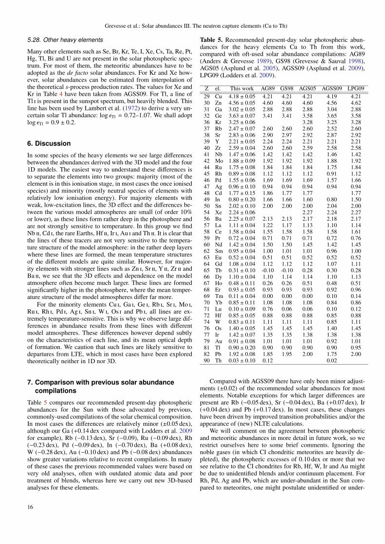
Grevesse et al.: Solar abundances III. The neutron capture elements (Cu to Th)
5.28. Other heavy elements
Many other elements such as Se, Br, Kr, Te, I, Xe, Cs, Ta, Re, Pt,Hg, Tl, Bi and U are not present in the solar photospheric spec-trum. For most of them, the meteoritic abundances have to beadopted as the de facto solar abundances. For Kr and Xe how-ever, solar abundances can be estimated from interpolation ofthe theoretical s-process production rates. The values for Xe andKr in Table 4 have been taken from AGSS09. For Tl, a line ofTl i is present in the sunspot spectrum, but heavily blended. Thisline has been used by Lambert et al. (1972) to derive a very un-certain solar Tl abundance: log εTl = 0.72–1.07. We shall adoptlog εTl = 0.9 ± 0.2.
6. Discussion
In some species of the heavy elements we see large differencesbetween the abundances derived with the 3D model and the four1D models. The easiest way to understand these differences isto separate the elements into two groups: majority (most of theelement is in this ionisation stage, in most cases the once ionisedspecies) and minority (mostly neutral species of elements withrelatively low ionisation energy). For majority elements withweak, low-excitation lines, the 3D effect and the differences be-tween the various model atmospheres are small (of order 10%or lower), as these lines form rather deep in the photosphere andare not strongly sensitive to temperature. In this group we findNb ii, Cd i, the rare Earths, Hf ii, Ir i, Au i and Th ii. It is clear thatthe lines of these tracers are not very sensitive to the tempera-ture structure of the model atmosphere: in the rather deep layerswhere these lines are formed, the mean temperature structuresof the different models are quite similar. However, for major-ity elements with stronger lines such as Zn i, Sr ii, Y ii, Zr ii andBa ii, we see that the 3D effects and dependence on the modelatmosphere often become much larger. These lines are formedsignificantly higher in the photosphere, where the mean temper-ature structure of the model atmospheres differ far more.
For the minority elements Cu i, Ga i, Ge i, Rb i, Sr i, Mo i,Ru i, Rh i, Pd i, Ag i, Sn i, W i, Os i and Pb i, all lines are ex-tremely temperature-sensitive. This is why we observe large dif-ferences in abundance results from these lines with differentmodel atmospheres. These differences however depend subtlyon the characteristics of each line, and its mean optical depthof formation. We caution that such lines are likely sensitive todepartures from LTE, which in most cases have been exploredtheoretically neither in 1D nor 3D.
7. Comparison with previous solar abundancecompilations
Table 5 compares our recommended present-day photosphericabundances for the Sun with those advocated by previous,commonly-used compilations of the solar chemical composition.In most cases the differences are relatively minor (±0.05 dex),although our Ga (+0.14 dex compared with Lodders et al. 2009for example), Rb (−0.13 dex), Sr (−0.09), Ru (−0.09 dex), Rh(−0.23 dex), Pd (−0.09 dex), In (−0.70 dex), Ba (+0.08 dex),W (−0.28 dex), Au (−0.10 dex) and Pb (−0.08 dex) abundancesshow greater variations relative to recent compilations. In manyof these cases the previous recommended values were based onvery old analyses, often with outdated atomic data and poortreatment of blends, whereas here we carry out new 3D-basedanalyses for these elements.
Table 5. Recommended present-day solar photospheric abun-dances for the heavy elements Cu to Th from this work,compared with oft-used solar abundance compilations: AG89(Anders & Grevesse 1989), GS98 (Grevesse & Sauval 1998),AGS05 (Asplund et al. 2005), AGSS09 (Asplund et al. 2009),LPG09 (Lodders et al. 2009).
Z el. This work AG89 GS98 AGS05 AGSS09 LPG0929 Cu 4.18 ± 0.05 4.21 4.21 4.21 4.19 4.2130 Zn 4.56 ± 0.05 4.60 4.60 4.60 4.56 4.6231 Ga 3.02 ± 0.05 2.88 2.88 2.88 3.04 2.8832 Ge 3.63 ± 0.07 3.41 3.41 3.58 3.65 3.5836 Kr 3.25 ± 0.06 3.28 3.25 3.2837 Rb 2.47 ± 0.07 2.60 2.60 2.60 2.52 2.6038 Sr 2.83 ± 0.06 2.90 2.97 2.92 2.87 2.9239 Y 2.21 ± 0.05 2.24 2.24 2.21 2.21 2.2140 Zr 2.59 ± 0.04 2.60 2.60 2.59 2.58 2.5841 Nb 1.47 ± 0.06 1.42 1.42 1.42 1.46 1.4242 Mo 1.88 ± 0.09 1.92 1.92 1.92 1.88 1.9244 Ru 1.75 ± 0.08 1.84 1.84 1.84 1.75 1.8445 Rh 0.89 ± 0.08 1.12 1.12 1.12 0.91 1.1246 Pd 1.55 ± 0.06 1.69 1.69 1.69 1.57 1.6647 Ag 0.96 ± 0.10 0.94 0.94 0.94 0.94 0.9448 Cd 1.77 ± 0.15 1.86 1.77 1.77 1.7749 In 0.80 ± 0.20 1.66 1.66 1.60 0.80 1.5050 Sn 2.02 ± 0.10 2.00 2.00 2.00 2.04 2.0054 Xe 2.24 ± 0.06 2.27 2.24 2.2756 Ba 2.25 ± 0.07 2.13 2.13 2.17 2.18 2.1757 La 1.11 ± 0.04 1.22 1.17 1.13 1.10 1.1458 Ce 1.58 ± 0.04 1.55 1.58 1.58 1.58 1.6159 Pr 0.72 ± 0.04 0.71 0.71 0.71 0.72 0.7660 Nd 1.42 ± 0.04 1.50 1.50 1.45 1.42 1.4562 Sm 0.95 ± 0.04 1.00 1.01 1.01 0.96 1.0063 Eu 0.52 ± 0.04 0.51 0.51 0.52 0.52 0.5264 Gd 1.08 ± 0.04 1.12 1.12 1.12 1.07 1.1165 Tb 0.31 ± 0.10 -0.10 -0.10 0.28 0.30 0.2866 Dy 1.10 ± 0.04 1.10 1.14 1.14 1.10 1.1367 Ho 0.48 ± 0.11 0.26 0.26 0.51 0.48 0.5168 Er 0.93 ± 0.05 0.93 0.93 0.93 0.92 0.9669 Tm 0.11 ± 0.04 0.00 0.00 0.00 0.10 0.1470 Yb 0.85 ± 0.11 1.08 1.08 1.08 0.84 0.8671 Lu 0.10 ± 0.09 0.76 0.06 0.06 0.10 0.1272 Hf 0.85 ± 0.05 0.88 0.88 0.88 0.85 0.8874 W 0.83 ± 0.11 1.11 1.11 1.11 0.85 1.1176 Os 1.40 ± 0.05 1.45 1.45 1.45 1.40 1.4577 Ir 1.42 ± 0.07 1.35 1.35 1.38 1.38 1.3879 Au 0.91 ± 0.08 1.01 1.01 1.01 0.92 1.0181 Tl 0.90 ± 0.20 0.90 0.90 0.90 0.90 0.9582 Pb 1.92 ± 0.08 1.85 1.95 2.00 1.75 2.0090 Th 0.03 ± 0.10 0.12 0.02
Compared with AGSS09 there have only been minor adjust-ments (±0.02) of the recommended solar abundances for mostelements. Notable exceptions for which larger differences arepresent are Rb (−0.05 dex), Sr (−0.04 dex), Ba (+0.07 dex), Ir(+0.04 dex) and Pb (+0.17 dex). In most cases, these changeshave been driven by improved transition probabilities and/or theappearance of (new) NLTE calculations.
We will comment on the agreement between photosphericand meteoritic abundances in more detail in future work, so werestrict ourselves here to some brief comments. Ignoring thenoble gases (in which CI chondritic meteorites are heavily de-pleted), the photospheric excesses of 0.10 dex or more that wesee relative to the CI chondrites for Rb, Hf, W, Ir and Au mightbe due to unidentified blends and/or continuum placement. ForRh, Pd, Ag and Pb, which are under-abundant in the Sun com-pared to meteorites, one might postulate unidentified or under-
16

Grevesse et al.: Solar abundances III. The neutron capture elements (Cu to Th)
estimated NLTE effects: the photospheric lines we have used ofRh i, Pd i, Ag i and Pb i are rather low-excitation lines of minorityspecies, so are expected to be prone to NLTE effects.
8. Conclusions
In this paper we have redetermined the solar abundances of al-most every element from Cu to Th, using a new, highly realistic3D hydrodynamic model of the solar atmosphere. In most caseswe have based our determination on a full reanalysis of the rele-vant lines in the solar spectrum, including the latest atomic dataand extremely demanding line selection. We have accountedfor departures from LTE wherever such corrections exist. Insome cases, where other authors have already performed verydetailed and careful analyses based on full spectrum synthesis,we have computed the net impact on the relevant lines of usingour 3D model, and adjusted the previous 1D results accordingly.Together with the results of Papers I and II, the results we presenthere make up the first fully complete, detailed and homogeneousanalysis of the medium-and-heavy-element (Z > 8) compositionof the Sun.
Acknowledgements. We are deeply indebted to Maria Bergemann (Sr i, Sr ii andBa ii) and Yoichi Takeda (Zn i) for providing NLTE corrections for some ofour lines on request. We also thank Chris Sneden, Jim Lawler, Emile Biemontand Jean-Francois Wyart for providing their recent works prior to publica-tion, Glenn Wahlgren for helpful discussions regarding our Au i line and RemoCollet, Regner Trampedach and Wolfgang Hayek for other discussions. NG, PSand MA variously thank the Max Planck Institut fur Astrophysik, Garching,the Centre Spatial de Liege, the Department of Astrophysics, Geophysics andOceanography, University of Liege and Mount Stromlo Observatory for sup-port and hospitality during the production of this paper. We acknowledge fur-ther support from the Royal Belgian Observatory (NG), IAU Commission 46,the Lorne Trottier Chair in Astrophysics, the (Canadian) Institute for ParticlePhysics, the Banting Fellowship scheme as administered by the Natural Scienceand Engineering Research Council of Canada, the UK Science & TechnologyFacilities Council (PS) and the Australian Research Council (MA).
References
Allende Prieto, C., Barklem, P. S., Asplund, M., & Ruiz Cobo, B. 2001, ApJ,558, 830
Anders, E., & Grevesse, N. 1989, Geochim. Cosmochim. Acta, 53, 197Asplund, M. 2005, ARA&A, 43, 481Asplund, M., Gustafsson, B., Kieselman, D., & Eriksson, K. 1997, A&A, 318,
521Asplund, M., Nordlund, A., Trampedach, R., Allende Prieto, C., & Stein, R. F.
2000, A&A, 359, 729Asplund, M., Grevesse, N., & Sauval, A. J. 2005, in ASP Conf. Ser. 336, ed. T.
G. Barnes III & F. N. Bash (Astron. Soc. Pac., San Francisco), 25Asplund, M., Grevesse, N., Sauval, A. J., & Scott, P. 2009, ARA&A, 47, 481
(AGSS09)Banerjee, A., Das, D., & Natarajan, V. 2004, Europhys. Lett., 65, 172Barklem, P. S., & O’Mara, B. J. 2000, MNRAS, 311, 535Barklem, P. S., Piskunov, N., & O’Mara, B. J. 2000, A&AS 142, 467Beacham, J. R. & Andrew, K. L. 1971, JOSA, 61, 231Beck, D. R. 1992, Phys. Rev. A, 45, 1399Bielski, A. 1975, JQSRT, 15, 463Biemont, E., & Godefroid, M. 1980a, Phys. Scr, 22, 231Biemont, E., & Godefroid, M. 1980b, A&A, 84, 361Biemont, E., Grevesse, N., Hannaford, P., & Lowe, R.M. 1981, ApJ, 248, 867Biemont, E., Grevesse, N., Kwiatkowski, M. & Zimmermann, P. 1982, A&A,
108, 127Biemont, E., Grevesse, N., Hannaford, P., Lowe, R.M., & Whaling, W. 1983,
ApJ, 275, 889Biemont, E., Lynga, C., Li, Z. S., et al. 1999, MNRAS 303, 721Biemont, E., Garnir, H. P., Palmeri, P., Li, Z. S., & Svanberg, S. 2000, MNRAS,
312, 116Biemont, E., Blagoev, K., Engstrom, L., et al. 2011, MNRAS, 414, 3350Bize, S., Sortais, Y., Santos, M. S., et al. 1999, Europhys. Lett., 45, 558Bord, D. J., & Cowley, C. R. 2001, Bull. Amer. Astron. Soc. 33, 1433Bord, D. J., & Cowley, C. R. 2002, Sol. Phys., 211, 3
Brix, P., Kopfermann, H., Martin, R., & Walcher, W. 1951, Z. Phys., 130, 88Burbidge, E. M., Burbidge, G. R., Fowler, W. A., & Hoyle, F. 1957, Rev. Mod.
Phys., 29, 547Busso, M., Gallino, R., Lambert, D. L., Travaglio, C., & Smith, V. V. 2001, ApJ,
557, 802Butcher, H. R. 1987, Nature, 328, 127Caffau, E., Sbordone, L., Ludwig, H.-G., et al. 2008, A&A, 483, 591Caffau, E., Faraggiana, R., Ludwig, H.-G., Bonifacio, P., & Steffen, M., 2011a,
Astron. Nachr. 332, 128Caffau, E., Ludwig, H.-G., Steffen, M., Freytag, B., & Bonifacio, P. 2011b, Sol.
Phys. 268, 255Cameron, A. G. W. 1957, AJ, 62, 9Carlsson, J., Sturesson, L., & Svanberg, S. 1989, Z. Phys. D 11, 287Carlsson, J., Jonsson, P., & Sturesson, L. 1990, Z. Phys. D, 16, 87Cayrel, R., Hill, V., Beers, T. C., et al. 2001, Nature, 409, 691Chan, Y. W., Childs, W. J., & Goodman, L. S. 1968, Phys. Rev., 173, 107Civis, S., Matulkova, I., Cihelka, et al. 2010, Phys. Rev. A, 82, 022502Colarusso, P., Lebeault-Dorget, M. A., & Simart, B. 1997, Phys. Rev. A 55, 1526Corliss, C. H., & Bozman, W. R. 1962, NBS Monograph 53Crawford, M. F., Schawlow, A. L., Gray, W. M., & Kelly, F. M. 1949, Phys. Rev.,
75, 1112Cunningham, P. T. & Link, J. K. 1967, JOSA, 57, 1000Davidson, M. D., Snoek, L. C, Volten, H., & Donszelmann, A. 1992, A&A, 255,
457Delbouille, L., Neven, L., & Roland, G. 1973, Atlas photometrique du spectre
solaire de λ3000 a λ10000 (Institut d’Astrophysique, Universite de Liege)Delbouille, L., Roland, G., Brault, J. W., & Testerman, L. 1981, Photometric
Atlas of the Solar Spectrum from 1850 to 10000 cm−1 (Kitt Peak NationalObservatory, Tucson)
Den Hartog, E. A., Duquette, D. W. & Lawler, J. E. 1987, JOSA, B4, 48Den Hartog, E. A., Lawler, J. E., Sneden, C., & Cowan, J. J. 2003, ApJS, 148,
543Den Hartog, E. A., Lawler, J. E., Sneden, C., & Cowan, J. J. 2006, ApJS, 167,
292Dinneen, T. P., Berrah Mansour, N., Kurtz, C., & Young, L. 1991, Phys. Rev. A,
43, 4824Drake, S., & Aller, L. H. 1976, Proc. Nat. Acad. Sci. USA, 73, 269Duquette, D. W., & Lawler, J. E. 1985 JOSAB, 2, 1948Engleman, R., Litzen, U., Lundberg, H., & Wyart, J.-F. 1998, Phys. Scr, 57, 345Fischer, W., Huhnermann, H., & Kollath, K.-J. 1967, Z. Phys. 200, 158Fivet, V., Quinet, P., Palmeri, P., et al. 2009, MNRAS, 396, 2124Frebel, A., Christlieb, N., Norris, J. E., et al. 2007, ApJ, 660, L117Gaarde, M. B., Zerne, R., Caiyan, L., et al. 1994, Phys. Rev. A, 50, 209Gallagher, A. 1967, Phys. Rev., 157, 24Garcia, G., & Campos, J. 1988, JQSRT, 39, 477Golovin, A. F. & Striganov, A. R. 1968, Sov. Phys. Usp., 10, 658Gonzalez, G. 2006, MNRAS, 371, 781Gonzalez, A. M., Ortiz, M., & Campos, J. 1997, JQSRT, 57, 825Gopka, V. F., Yushchenko, A. V., Shavrina, A. V., Andrievsky, S. M., &
Chernysheva, L. V. 2001, KFNT 17, 37Goriely, S., Bauswein, A., & Janka, H.-T. 2011, ApJ, 738, L32Gough, D.S., Hannaford, P., & Lowe, R. M. 1983, J. Phys. B 16, 785Gratton, R. G., & Sneden, C. 1994, A&A, 287, 927Grevesse, N. 1984, Phys. Script. T8, 49Grevesse, N., & Sauval, A.J. 1998, Space Sci. Rev., 85, 161Grevesse, N., Boury, A., & Blanquet, G. 1968, in Origin and Distribution of the
Elements, ed. L. H. Ahrens, Pergamon Press, New York, 177Guern, Y., & Lotrian, J. 1980, JQSRT, 24, 133Gustafsson, B., Edvardsson, B., Eriksson, K., et al. 2008, A&A, 486, 951Hannaford, P. & McDonald, D. C. 1978, J. Phys. B 11, 1177Hannaford, P. & Lowe, R. M. 1983, Optical Engineering 22, 532Hannaford, P., Larkins, P. L., & Lowe, R.M. 1981, J. Phys. B 14, 2321Hannaford, P., Lowe, R. M., Grevesse, N., Biemont, E., & Whaling, W. 1982,
ApJ, 261, 736Hannaford, P., Lowe, R. M., Biemont, E., & Grevesse, N. 1985, A&A, 143, 447Hauge, O. 1972a, Sol. Phys. 26, 263Hauge, O. 1972b, Sol. Phys. 26, 276Holweger, H., & Muller, E. A. 1974, Sol. Phys., 39, 19Holweger, H., & Werner, K. 1982, Sol. Phys., 81, 3Hughes, R. H. 1961, Phys. Rev., 121, 499Ivarsson, S., Andersen, J., Nordstrom, B., et al. 2003, A&A, 409, 1141Jackson, D., & Kuhn, H. 1937, Proc. Roy. Soc. London, Ser. A, 158, 372Karakas, A. I., Garcıa-Hernandez, D. A., & Lugaro, M. 2012, ApJ, 751, 8Kerkhoff, H., Schmidt, M., & Zimmermann, P. 1980, Z. Phys. A, 298, 249Kling, R., & Kock, M. 1999, JQSRT, 62, 129Kobayashi, C. & Nakasato, N. 2011, ApJ, 729, 16Kock, M., & Richter, J. 1968, Z. Astr., 69, 180Kurucz, R. L. 1998 (http://kurucz.harvard.edu/)
17
Grevesse et al.: Solar abundances III. The neutron capture elements (Cu to Th)
Kurz, N., Dietrich, M. R., Shu, Gang, et al. 2008, Phys. Rev. A, 77, 060501Kuske, P., Kirchner, N., Wittmann, W., Andra, H. J., & Kaiser, D. 1978, Phys.
Lett. A, 64, 377Kwiatkowski, M., Zimmermann, P., Biemont,E., & Grevesse, N. 1982, A&A,
112, 337Kwiatkowski, M., Zimmermann, P., Biemont,E., & Grevesse, N. 1984, A&A,
135, 59Lambert, D. L., & Mallia, E. A. 1968, MNRAS, 140, 13Lambert, D. L., Mallia, E. A., & Warner, B. 1969, MNRAS, 142, 71Lambert, D. L., Mallia, E. A., & Smith, G. 1972, Sol. Phys., 26, 250Lawler, J. E., Whaling, W., & Grevesse, N. 1990, Nature, 346, 635Lawler, J. E., Bonvallet, G., & Sneden, C. 2001a, ApJ, 556, 452Lawler, J. E., Wickliffe, M. E., Den Hartog, E. A., & Sneden, C. 2001b, ApJ,
563, 1075Lawler, J. E., Wickliffe, M. E., Cowley, C. R., & Sneden, C. 2001c, ApJS, 137,
341Lawler, J. E., Sneden, C., & Cowan, J. J. 2004, ApJ, 604, 850Lawler, J. E., Den Hartog, E. A., Sneden, C., & Cowan, J. J. 2006, ApJS, 162,
227Lawler, J. E., Den Hartog, E. A., Labby, Z. E., et al. 2007, ApJS, 169, 120Lawler, J. E., Sneden, C., Cowan, et al. 2008, ApJS, 178, 71Lawler, J. E., Sneden, C., Cowan, J., Ivans, I., & Den Hartog, E. A. 2009, ApJS,
182, 51Learner, R. C. M., Davies, J., & Thorne, A. P. 1991, MNRAS, 248, 414Li, R., Rehse, S. J., Scholl, T. J., et al. 2007, Can. J. Phys., 85, 1343Ljung, G., Nilsson, H., Asplund, M.,& Johansson, S. 2006, A&A, 456, 1181Lodders, K., Palme, H., & Gail, H.-P. 2009, Landolt Bornstein, New Series, Vol.
VI/4B, Chap. 4.4, Abundances of the Elements in the Solar System, ed. J. E.Trumper (Springer-Verlag, Berlin), 560–630
Lotrian, J., Cariou, J., & Johannin-Gilles, A. 1976, JQSRT, 16, 315Mashonkina, L. I., & Gehren, T. 2000, A&A, 364, 249Mashonkina, L. I., & Gehren, T. 2001, A&A, 376, 232Mashonkina, L. I., Gehren, T., & Bikmaiev, I. F. 1999, A&A, 343, 519Mashonkina, L. I., Ryabtsev, A. & Frebel, A. 2012, A&A, 540, A98Meggers, W. F., Corliss, C. H., & Scribner, B. F. 1961, National Bureau of
Standards Monograph 32, U.S. Dept. of Commerce, Washington USAMigdalek, J. & Baylis, W. E. 1987, Can. J. Phys., 65, 1612Morton, D C. 2000, ApJS, 130, 403Mucciarelli, A., Caffau, E., Freytag, B., Ludwig, H.-G., & Bonifacio, P.C. 2008,
A&A, 484, 841Neckel, H., & Labs, D. 1984, Sol. Phys., 90, 205; erratum Sol. Phys., 92, 391Nez, F., Biraben, F., Felder, R., & Millerioux, Y. 1993, Opt. Communications,
102, 432Nilsson, H. & Ivarsson, S. 2008, A&A, 492, 609Nilsson, H., Zhang, Z. G., Lundberg, H., Johansson, S., & Nordstrom, B. 2002,
A&A, 382, 368Nilsson, H., Hartman, H., Engstrom, L., et al. 2010, A&A, 511, 16Pereira, T. M. D., Asplund, M., Collet, R., et al. 2013, A&A, 554, A118Pickering, J. C., & Semeniuk, J. I. 1995, MNRAS, 274, L37Pignatari, M., Gallino, R., Meynet, G., et al. 2008, ApJ, 687, L95Pinnington, E. H., Berends, R. W. & Lumsden, M. 1995, J. Phys. B, 28, 2095Quinet, P., Palmeri, P., Biemont, E., et al. 2006, A&A, 448, 1207Rapol, U. D., Krishna, A., & Natarajan, V. 2003, Eur. Phys. J. D, 23, 185Rehse, S. J., Li, R., Scholl, T. J., et al. 2006, Can. J. Phys., 84, 723Roederer, I. U., Preston, G. W., Thompson, I. B., Shectman, S. A., & Sneden, C.
2014, ApJ, 784, 158Ross, J. E., & Aller, L. H. 1970, Proc. Nat. Acad. Sci. 66, 983Ross, J. E., & Aller, L. H. 1972, Sol. Phys. 25, 30Ross, J. E., & Aller, L. H. 1976, Science 191, 1223Rutten, R. J. 1978, Sol. Phys., 56, 237Rutten, R. J. & Kostik, R. I. 1982, A&A, 115, 104Scott, P., Grevesse, N., Asplund, M., et al. 2014a, submitted to A&A (Paper I).Scott, P., Asplund, M., Grevesse, N., Bergemann, M. & Sauval, A. J. 2014b,
submitted to A&A (Paper II).Shi, J. R., Gehren, T., Zeng, J. L., Mashonkina, L. & Zhao, G. 2014, ApJ, 782,
80Simsarian, J. E., Orozco, L. A., Sprouse, G. D., & Zhao, W. Z. 1998, Phys. Rev.
A, 57, 2448Sneden, C. & Crocker, D. A. 1988, ApJ, 335, 406Sneden, C., Cowan, J. J., Lawler, J. E., et al. 2003, ApJ, 591, 936Sneden, C., Cowan, J. J., & Gallino, R. 2008, ARA&A, 46, 241Sneden, C., Lawler, J. E., Cowan, J., Ivans, I., & Den Hartog, E. 2009, ApJS,
182, 80Takeda, Y., Hashimoto, O., Taguchi, H., et al. 2005, PASJ, 57, 751Trapp, S., Marx, G., Tommaseo, G., et al. 2000, Hyperfine Interactions, 127, 57Truran, J. W. 1981, A&A, 97, 391Unsold, A. 1955, Physik der Sternatmospharen, mit besonderer
Berucksichtigung der Sonne, 2nd edn. (Springer, Berlin)
van Hove, M., Borghs, G., de Bisschop, P., & Silverans, R. E. 1982, J. Phys. B,15, 1805
van Hove, M., Borghs, G., de Bisschop, P., & Silverans, R. E. 1985, Z. Phys. A,321, 215
Veer, W. E. v.d., Blonk, D. P. v.d., Donszelmann, A., & Snoek, C. 1990, A&A,231, 277
Velichko, A. B., Mashonkina, L. I., & Nilsson, H. 2010, Astron. Lett. 36, 664Velichko, A. B., Mashonkina, L. I., & Nilsson, H. 2011, Astron. Lett. 37, 440Villemoes, P., Arnesen, A., Heijkenskjold, F.; Wannstrom, A. 1993, J. Phys. B,
26, 4289Vitas, N., Vince, I., Lugaro, M., et al. 2008, MNRAS, 384, 370Volz, U., & Schmoranzer, H. 1996, Phys. Scr. 65, 48Wannstrom, A., Vogel, O., Arnesen, A & Hallin, R. 1988, Phys. Scr., 38, 564Wanajo, S. 2013, ApJ, 770, L22Wendt, K., Ahmad, S. A., Buchinger, F., et al. 1984, Z. Phys. A, 318, 125Wessel, G., & Lew, H. 1953, Phys. Rev., 92, 641Whaling, W., & Brault, J. W. 1988, Phys. Scr., 38, 707Whaling, W., Hannaford, P., Lowe, R. M., Biemont, E., & Grevesse, N. 1984,
JQSRT, 32, 69Wickliffe, M. E., Salih, S., & Lawler, J. E. 1994, JQSRT, 51, 545Xu, H. L., Sun, Z. W., Dai, Z. W., et al. 2006, A&A, 452, 357Xu, H. L., Svanberg, S., Quinet, P., Palmeri, P. & Biemont, E. 2007, JQSRT, 104,
52Ye, J., Swartz, S., Jungner, P., & Hall, J. L. 1996, Opt. Lett., 21, 1280Youssef, N. H. 1986, A&A, 164, 395Youssef, N. H., & Khalil, N. M. 1988, A&A, 203, 378Youssef, N. H., Donszelmann, A., & Grevesse, N. 1990, A&A, 239, 367
18
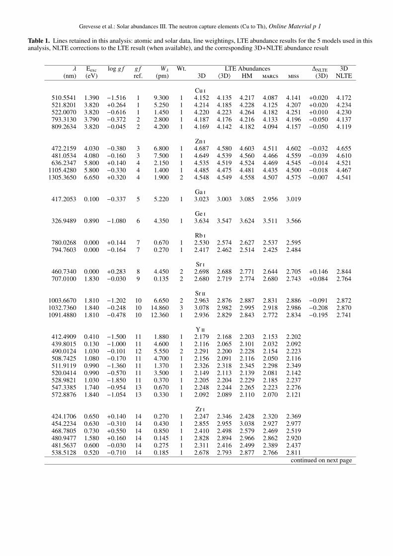
Grevesse et al.: Solar abundances III. The neutron capture elements (Cu to Th), Online Material p 1
Table 1. Lines retained in this analysis: atomic and solar data, line weightings, LTE abundance results for the 5 models used in thisanalysis, NLTE corrections to the LTE result (when available), and the corresponding 3D+NLTE abundance result
λ Eexc log g f g f Wλ Wt. LTE Abundances ∆NLTE 3D(nm) (eV) ref. (pm) 3D 〈3D〉 HM marcs miss (3D) NLTE
Cu i510.5541 1.390 −1.516 1 9.300 1 4.152 4.135 4.217 4.087 4.141 +0.020 4.172521.8201 3.820 +0.264 1 5.250 1 4.214 4.185 4.228 4.125 4.207 +0.020 4.234522.0070 3.820 −0.616 1 1.450 1 4.220 4.223 4.264 4.182 4.251 +0.010 4.230793.3130 3.790 −0.372 2 2.800 1 4.187 4.176 4.216 4.133 4.196 −0.050 4.137809.2634 3.820 −0.045 2 4.200 1 4.169 4.142 4.182 4.094 4.157 −0.050 4.119
Zn i472.2159 4.030 −0.380 3 6.800 1 4.687 4.580 4.603 4.511 4.602 −0.032 4.655481.0534 4.080 −0.160 3 7.500 1 4.649 4.539 4.560 4.466 4.559 −0.039 4.610636.2347 5.800 +0.140 4 2.150 1 4.535 4.519 4.524 4.469 4.545 −0.014 4.521
1105.4280 5.800 −0.330 4 1.400 1 4.485 4.475 4.481 4.435 4.500 −0.018 4.4671305.3650 6.650 +0.320 4 1.900 2 4.548 4.549 4.558 4.507 4.575 −0.007 4.541
Ga i417.2053 0.100 −0.337 5 5.220 1 3.023 3.003 3.085 2.956 3.019
Ge i326.9489 0.890 −1.080 6 4.350 1 3.634 3.547 3.624 3.511 3.566
Rb i780.0268 0.000 +0.144 7 0.670 1 2.530 2.574 2.627 2.537 2.595794.7603 0.000 −0.164 7 0.270 1 2.417 2.462 2.514 2.425 2.484
Sr i460.7340 0.000 +0.283 8 4.450 2 2.698 2.688 2.771 2.644 2.705 +0.146 2.844707.0100 1.830 −0.030 9 0.135 2 2.680 2.719 2.774 2.680 2.743 +0.084 2.764
Sr ii1003.6670 1.810 −1.202 10 6.650 2 2.963 2.876 2.887 2.831 2.886 −0.091 2.8721032.7360 1.840 −0.248 10 14.860 3 3.078 2.982 2.995 2.918 2.986 −0.208 2.8701091.4880 1.810 −0.478 10 12.360 1 2.936 2.829 2.843 2.772 2.834 −0.195 2.741
Y ii412.4909 0.410 −1.500 11 1.880 1 2.179 2.168 2.203 2.153 2.202439.8015 0.130 −1.000 11 4.600 1 2.116 2.065 2.101 2.032 2.092490.0124 1.030 −0.101 12 5.550 2 2.291 2.200 2.228 2.154 2.223508.7425 1.080 −0.170 11 4.700 1 2.156 2.091 2.116 2.050 2.116511.9119 0.990 −1.360 11 1.370 1 2.326 2.318 2.345 2.298 2.349520.0414 0.990 −0.570 11 3.500 1 2.149 2.113 2.139 2.081 2.142528.9821 1.030 −1.850 11 0.370 1 2.205 2.204 2.229 2.185 2.237547.3385 1.740 −0.954 13 0.670 1 2.248 2.244 2.265 2.223 2.276572.8876 1.840 −1.054 13 0.330 1 2.092 2.089 2.110 2.070 2.121
Zr i424.1706 0.650 +0.140 14 0.270 1 2.247 2.346 2.428 2.320 2.369454.2234 0.630 −0.310 14 0.430 1 2.855 2.955 3.038 2.927 2.977468.7805 0.730 +0.550 14 0.850 1 2.410 2.498 2.579 2.469 2.519480.9477 1.580 +0.160 14 0.145 1 2.828 2.894 2.966 2.862 2.920481.5637 0.600 −0.030 14 0.275 1 2.311 2.416 2.499 2.389 2.437538.5128 0.520 −0.710 14 0.185 1 2.678 2.793 2.877 2.766 2.811
continued on next page
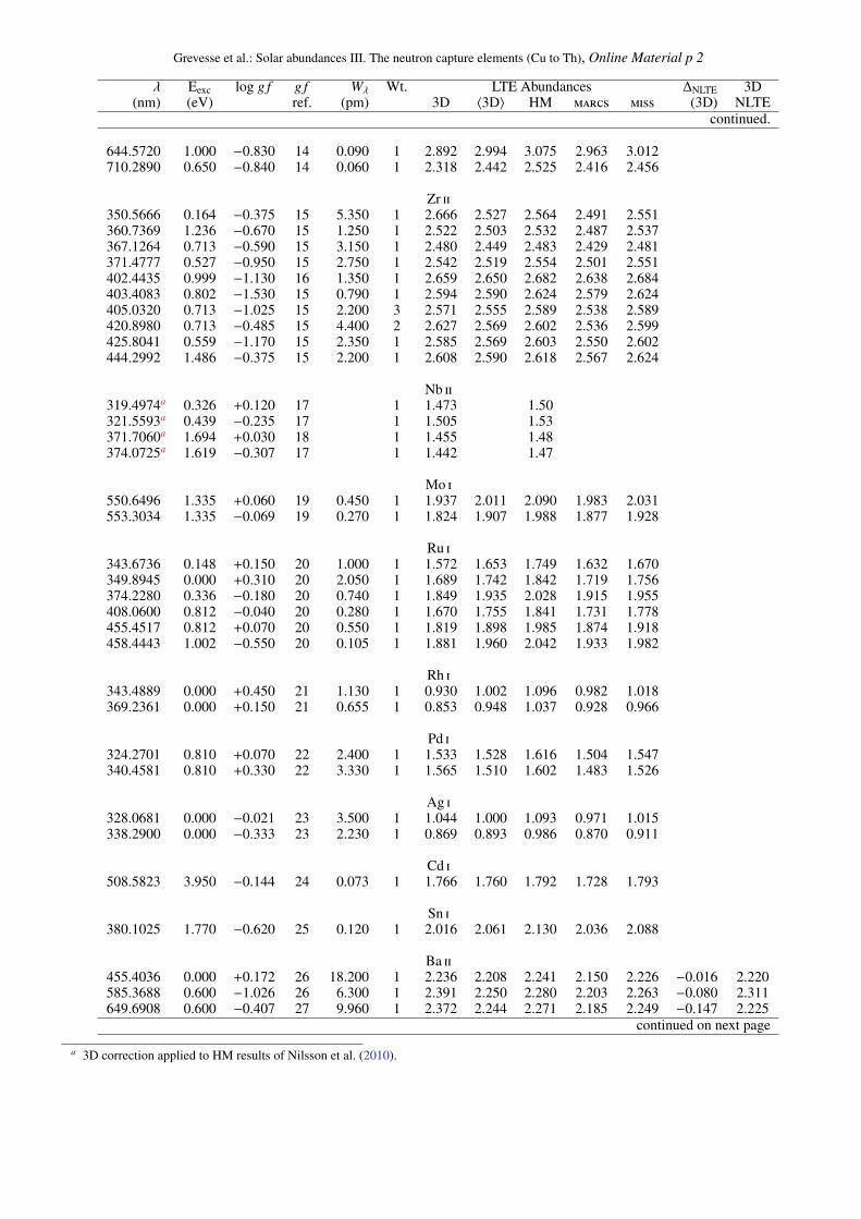
Grevesse et al.: Solar abundances III. The neutron capture elements (Cu to Th), Online Material p 2
λ Eexc log g f g f Wλ Wt. LTE Abundances ∆NLTE 3D(nm) (eV) ref. (pm) 3D 〈3D〉 HM marcs miss (3D) NLTE
continued.
644.5720 1.000 −0.830 14 0.090 1 2.892 2.994 3.075 2.963 3.012710.2890 0.650 −0.840 14 0.060 1 2.318 2.442 2.525 2.416 2.456
Zr ii350.5666 0.164 −0.375 15 5.350 1 2.666 2.527 2.564 2.491 2.551360.7369 1.236 −0.670 15 1.250 1 2.522 2.503 2.532 2.487 2.537367.1264 0.713 −0.590 15 3.150 1 2.480 2.449 2.483 2.429 2.481371.4777 0.527 −0.950 15 2.750 1 2.542 2.519 2.554 2.501 2.551402.4435 0.999 −1.130 16 1.350 1 2.659 2.650 2.682 2.638 2.684403.4083 0.802 −1.530 15 0.790 1 2.594 2.590 2.624 2.579 2.624405.0320 0.713 −1.025 15 2.200 3 2.571 2.555 2.589 2.538 2.589420.8980 0.713 −0.485 15 4.400 2 2.627 2.569 2.602 2.536 2.599425.8041 0.559 −1.170 15 2.350 1 2.585 2.569 2.603 2.550 2.602444.2992 1.486 −0.375 15 2.200 1 2.608 2.590 2.618 2.567 2.624
Nb ii319.4974a 0.326 +0.120 17 1 1.473 1.50321.5593a 0.439 −0.235 17 1 1.505 1.53371.7060a 1.694 +0.030 18 1 1.455 1.48374.0725a 1.619 −0.307 17 1 1.442 1.47
Mo i550.6496 1.335 +0.060 19 0.450 1 1.937 2.011 2.090 1.983 2.031553.3034 1.335 −0.069 19 0.270 1 1.824 1.907 1.988 1.877 1.928
Ru i343.6736 0.148 +0.150 20 1.000 1 1.572 1.653 1.749 1.632 1.670349.8945 0.000 +0.310 20 2.050 1 1.689 1.742 1.842 1.719 1.756374.2280 0.336 −0.180 20 0.740 1 1.849 1.935 2.028 1.915 1.955408.0600 0.812 −0.040 20 0.280 1 1.670 1.755 1.841 1.731 1.778455.4517 0.812 +0.070 20 0.550 1 1.819 1.898 1.985 1.874 1.918458.4443 1.002 −0.550 20 0.105 1 1.881 1.960 2.042 1.933 1.982
Rh i343.4889 0.000 +0.450 21 1.130 1 0.930 1.002 1.096 0.982 1.018369.2361 0.000 +0.150 21 0.655 1 0.853 0.948 1.037 0.928 0.966
Pd i324.2701 0.810 +0.070 22 2.400 1 1.533 1.528 1.616 1.504 1.547340.4581 0.810 +0.330 22 3.330 1 1.565 1.510 1.602 1.483 1.526
Ag i328.0681 0.000 −0.021 23 3.500 1 1.044 1.000 1.093 0.971 1.015338.2900 0.000 −0.333 23 2.230 1 0.869 0.893 0.986 0.870 0.911
Cd i508.5823 3.950 −0.144 24 0.073 1 1.766 1.760 1.792 1.728 1.793
Sn i380.1025 1.770 −0.620 25 0.120 1 2.016 2.061 2.130 2.036 2.088
Ba ii455.4036 0.000 +0.172 26 18.200 1 2.236 2.208 2.241 2.150 2.226 −0.016 2.220585.3688 0.600 −1.026 26 6.300 1 2.391 2.250 2.280 2.203 2.263 −0.080 2.311649.6908 0.600 −0.407 27 9.960 1 2.372 2.244 2.271 2.185 2.249 −0.147 2.225
continued on next page
a 3D correction applied to HM results of Nilsson et al. (2010).
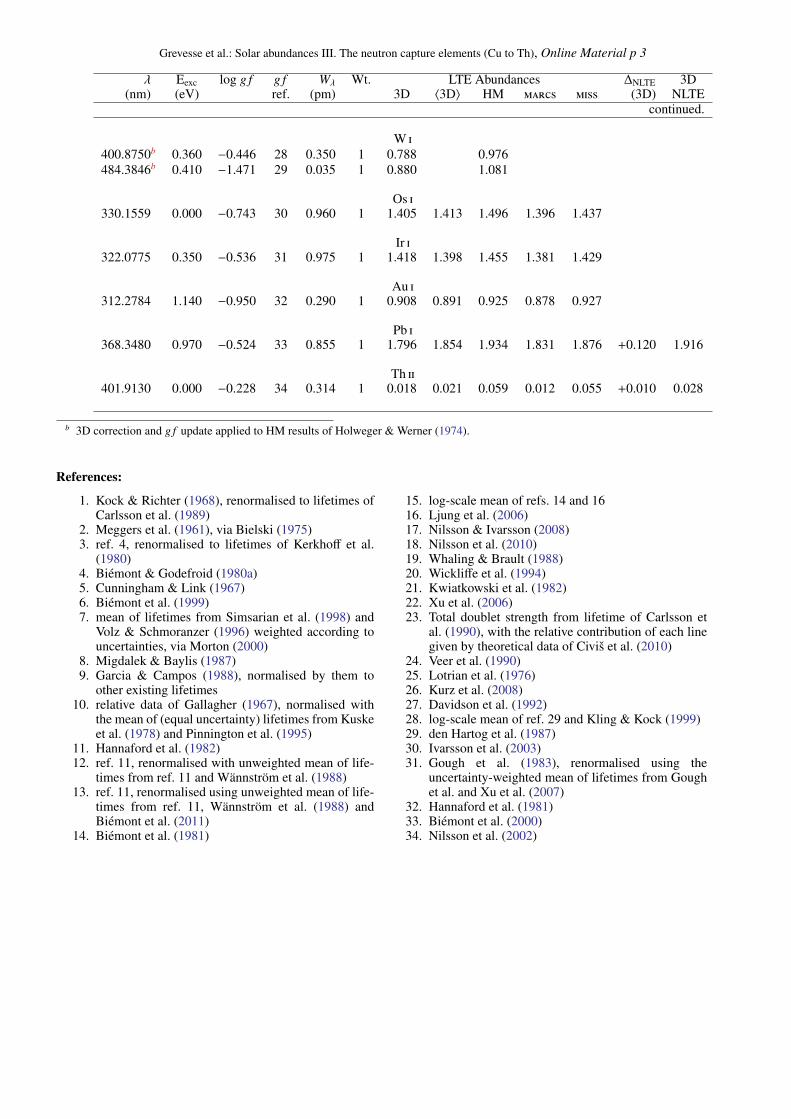
Grevesse et al.: Solar abundances III. The neutron capture elements (Cu to Th), Online Material p 3
λ Eexc log g f g f Wλ Wt. LTE Abundances ∆NLTE 3D(nm) (eV) ref. (pm) 3D 〈3D〉 HM marcs miss (3D) NLTE
continued.
W i400.8750b 0.360 −0.446 28 0.350 1 0.788 0.976484.3846b 0.410 −1.471 29 0.035 1 0.880 1.081
Os i330.1559 0.000 −0.743 30 0.960 1 1.405 1.413 1.496 1.396 1.437
Ir i322.0775 0.350 −0.536 31 0.975 1 1.418 1.398 1.455 1.381 1.429
Au i312.2784 1.140 −0.950 32 0.290 1 0.908 0.891 0.925 0.878 0.927
Pb i368.3480 0.970 −0.524 33 0.855 1 1.796 1.854 1.934 1.831 1.876 +0.120 1.916
Th ii401.9130 0.000 −0.228 34 0.314 1 0.018 0.021 0.059 0.012 0.055 +0.010 0.028
b 3D correction and g f update applied to HM results of Holweger & Werner (1974).
References:
1. Kock & Richter (1968), renormalised to lifetimes ofCarlsson et al. (1989)
2. Meggers et al. (1961), via Bielski (1975)3. ref. 4, renormalised to lifetimes of Kerkhoff et al.
(1980)4. Biemont & Godefroid (1980a)5. Cunningham & Link (1967)6. Biemont et al. (1999)7. mean of lifetimes from Simsarian et al. (1998) and
Volz & Schmoranzer (1996) weighted according touncertainties, via Morton (2000)
8. Migdalek & Baylis (1987)9. Garcia & Campos (1988), normalised by them to
other existing lifetimes10. relative data of Gallagher (1967), normalised with
the mean of (equal uncertainty) lifetimes from Kuskeet al. (1978) and Pinnington et al. (1995)
11. Hannaford et al. (1982)12. ref. 11, renormalised with unweighted mean of life-
times from ref. 11 and Wannstrom et al. (1988)13. ref. 11, renormalised using unweighted mean of life-
times from ref. 11, Wannstrom et al. (1988) andBiemont et al. (2011)
14. Biemont et al. (1981)
15. log-scale mean of refs. 14 and 1616. Ljung et al. (2006)17. Nilsson & Ivarsson (2008)18. Nilsson et al. (2010)19. Whaling & Brault (1988)20. Wickliffe et al. (1994)21. Kwiatkowski et al. (1982)22. Xu et al. (2006)23. Total doublet strength from lifetime of Carlsson et
al. (1990), with the relative contribution of each linegiven by theoretical data of Civis et al. (2010)
24. Veer et al. (1990)25. Lotrian et al. (1976)26. Kurz et al. (2008)27. Davidson et al. (1992)28. log-scale mean of ref. 29 and Kling & Kock (1999)29. den Hartog et al. (1987)30. Ivarsson et al. (2003)31. Gough et al. (1983), renormalised using the
uncertainty-weighted mean of lifetimes from Goughet al. and Xu et al. (2007)
32. Hannaford et al. (1981)33. Biemont et al. (2000)34. Nilsson et al. (2002)
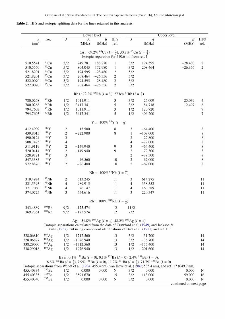
Grevesse et al.: Solar abundances III. The neutron capture elements (Cu to Th), Online Material p 4
Table 2. HFS and isotopic splitting data for the lines retained in this analysis.
Lower level Upper levelλ Iso. J A B HFS J A B HFS
(nm) (MHz) (MHz) ref. (MHz) (MHz) ref.
Cu i : 69.2% 63Cu (I = 32 ), 30.8% 65Cu (I = 3
2 )Isotopic separation for 510.6 nm from ref. 1
510.5541 63Cu 5/2 749.781 188.270 1 3/2 194.595 −28.480 2510.5560 65Cu 5/2 804.043 172.980 1 3/2 208.464 −26.356 2521.8201 63Cu 3/2 194.595 −28.480 2 5/2521.8201 65Cu 3/2 208.464 −26.356 2 5/2522.0070 63Cu 3/2 194.595 −28.480 2 3/2522.0070 65Cu 3/2 208.464 −26.356 2 3/2
Rb i : 72.2% 85Rb (I = 52 ), 27.8% 87Rb (I = 3
2 )
780.0268 85Rb 1/2 1011.911 3 3/2 25.009 25.039 4780.0268 87Rb 1/2 3417.341 5 3/2 84.718 12.497 6794.7603 85Rb 1/2 1011.911 3 1/2 120.720 7794.7603 87Rb 1/2 3417.341 5 1/2 406.200 7
Y ii : 100% 89Y (I = 12 )
412.4909 89Y 2 15.500 8 3 −64.400 8439.8015 89Y 2 −222.900 8 1 −108.000 8490.0124 89Y 3 2 −22.800 8508.7425 89Y 4 4 −29.000 8511.9119 89Y 2 −149.940 9 3 −64.400 8520.0414 89Y 2 −149.940 9 2 −79.300 8528.9821 89Y 3 2 −79.300 8547.3385 89Y 1 46.560 10 2 −67.000 8572.8876 89Y 2 −26.400 10 2 −67.000 8
Nb ii : 100% 93Nb (I = 92 )
319.4974 93Nb 2 513.245 11 3 614.275 11321.5593 93Nb 4 989.915 11 4 358.552 11371.7060 93Nb 4 76.147 11 4 160.389 11374.0725 93Nb 3 554.616 11 3 220.347 11
Rh i : 100% 103Rh (I = 12 )
343.4889 103Rh 9/2 −175.574 12 11/2369.2361 103Rh 9/2 −175.574 12 7/2
Ag i : 51.8% 107Ag (I = 12 ), 48.2% 109Ag (I = 1
2 )Isotopic separations calculated from the data of Crawford et al. (1949) and Jackson &
Kuhn (1937), but using component idetifications of Brix et al. (1951) and ref. 13
328.06810 107Ag 1/2 −1712.560 13 3/2 −31.700 14328.06827 109Ag 1/2 −1976.940 13 3/2 −36.700 14338.29000 107Ag 1/2 −1712.560 13 1/2 −175.400 14338.29018 109Ag 1/2 −1976.940 13 1/2 −201.600 14
Ba ii : 0.1% 130Ba (I = 0), 0.1% 132Ba (I = 0), 2.4% 134Ba (I = 0),6.6% 135Ba (I = 3
2 ), 7.9% 136Ba (I = 0), 11.2% 137Ba (I = 32 ), 71.7% 138Ba (I = 0)
Isotopic separations from Wendt et al. (1984; 455.4 nm), van Hove et al. (1982; 585.4 nm), and ref. 17 (649.7 nm)455.40334 130Ba 1/2 0.000 0.000 N 3/2 0.000 0.000 N455.40335 135Ba 1/2 3591.670 15 3/2 113.000 59.000 16455.40340 132Ba 1/2 0.000 0.000 N 3/2 0.000 0.000 N
continued on next page
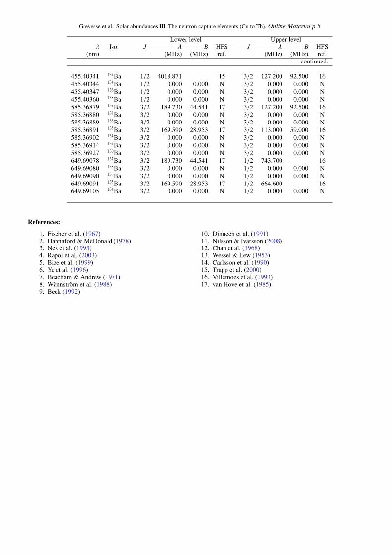
Grevesse et al.: Solar abundances III. The neutron capture elements (Cu to Th), Online Material p 5
Lower level Upper levelλ Iso. J A B HFS J A B HFS
(nm) (MHz) (MHz) ref. (MHz) (MHz) ref.continued.
455.40341 137Ba 1/2 4018.871 15 3/2 127.200 92.500 16455.40344 134Ba 1/2 0.000 0.000 N 3/2 0.000 0.000 N455.40347 136Ba 1/2 0.000 0.000 N 3/2 0.000 0.000 N455.40360 138Ba 1/2 0.000 0.000 N 3/2 0.000 0.000 N585.36879 137Ba 3/2 189.730 44.541 17 3/2 127.200 92.500 16585.36880 138Ba 3/2 0.000 0.000 N 3/2 0.000 0.000 N585.36889 136Ba 3/2 0.000 0.000 N 3/2 0.000 0.000 N585.36891 135Ba 3/2 169.590 28.953 17 3/2 113.000 59.000 16585.36902 134Ba 3/2 0.000 0.000 N 3/2 0.000 0.000 N585.36914 132Ba 3/2 0.000 0.000 N 3/2 0.000 0.000 N585.36927 130Ba 3/2 0.000 0.000 N 3/2 0.000 0.000 N649.69078 137Ba 3/2 189.730 44.541 17 1/2 743.700 16649.69080 138Ba 3/2 0.000 0.000 N 1/2 0.000 0.000 N649.69090 136Ba 3/2 0.000 0.000 N 1/2 0.000 0.000 N649.69091 135Ba 3/2 169.590 28.953 17 1/2 664.600 16649.69105 134Ba 3/2 0.000 0.000 N 1/2 0.000 0.000 N
References:
1. Fischer et al. (1967)2. Hannaford & McDonald (1978)3. Nez et al. (1993)4. Rapol et al. (2003)5. Bize et al. (1999)6. Ye et al. (1996)7. Beacham & Andrew (1971)8. Wannstrom et al. (1988)9. Beck (1992)
10. Dinneen et al. (1991)11. Nilsson & Ivarsson (2008)12. Chan et al. (1968)13. Wessel & Lew (1953)14. Carlsson et al. (1990)15. Trapp et al. (2000)16. Villemoes et al. (1993)17. van Hove et al. (1985)
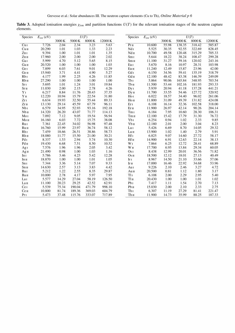
Grevesse et al.: Solar abundances III. The neutron capture elements (Cu to Th), Online Material p 6
Table 3. Adopted ionisation energies χion and partition functions U(T ) for the relevant ionisation stages of the neutron captureelements.
Species Eion (eV) U(T )3000 K 5000 K 8000 K 12000 K
Cu i 7.726 2.04 2.34 3.23 5.63Cu ii 20.290 1.01 1.03 1.33 2.23Zn i 9.394 1.00 1.01 1.01 1.35Zn ii 17.960 2.00 2.00 2.00 2.02Ga i 5.999 4.70 5.12 5.65 8.15Ga ii 20.520 1.00 1.00 1.00 1.03Ge i 7.899 6.03 7.61 9.01 12.29Ge ii 15.940 3.71 4.41 4.90 5.27Rb i 4.177 1.99 2.25 4.26 11.85Rb ii 27.290 1.00 1.00 1.00 1.00Sr i 5.695 1.01 1.24 3.01 19.84Sr ii 11.030 2.00 2.15 2.78 4.26Y i 6.217 8.84 11.76 20.43 37.35Y ii 12.220 10.94 15.79 22.54 31.80Zr i 6.634 19.93 32.50 55.44 89.33Zr ii 13.130 29.14 45.59 67.79 96.11Nb i 6.579 34.95 52.93 93.16 192.18Nb ii 14.320 26.20 43.07 71.77 114.13Mo i 7.092 7.12 9.05 19.54 56.94Mo ii 16.160 6.03 7.72 15.75 38.08Ru i 7.361 22.45 34.02 56.98 97.48Ru ii 16.760 15.99 23.97 36.74 58.12Rh i 7.459 18.66 26.51 38.86 58.73Rh ii 18.080 11.77 15.50 21.00 30.21Pd i 8.337 1.53 2.94 5.74 10.30Pd ii 19.430 6.68 7.51 8.50 10.52Ag i 7.576 1.96 1.96 2.05 3.42Ag ii 21.490 0.98 1.00 1.03 1.16In i 5.786 3.46 4.23 5.42 12.28In ii 18.870 1.00 1.00 1.01 1.05Sn i 7.344 3.36 5.14 7.07 9.33Sn ii 14.630 2.57 3.13 3.83 4.42Ba i 5.212 1.22 2.55 8.35 29.87Ba ii 10.000 2.78 4.17 5.97 7.95La i 5.577 14.29 27.04 58.19 126.50La ii 11.100 20.23 29.25 42.52 62.91Ce i 5.539 75.34 190.04 471.79 998.10Ce ii 10.800 81.74 189.36 369.03 604.79Pr i 5.473 37.48 115.76 333.07 717.89
Species Eion (eV) U(T )3000 K 5000 K 8000 K 12000 K
Pr ii 10.600 55.98 138.35 318.42 585.87Nd i 5.525 30.35 92.55 322.69 828.45Nd ii 10.700 49.58 120.48 315.29 705.33Sm i 5.644 18.22 38.24 108.47 299.28Sm ii 11.100 31.27 59.16 120.02 243.16Eu i 5.670 8.16 10.97 28.31 103.98Eu ii 11.240 12.49 15.87 23.96 42.00Gd i 6.150 34.56 59.41 135.19 318.79Gd ii 12.100 48.42 83.38 146.39 249.09Tb i 5.864 90.06 165.84 348.95 703.54Tb ii 11.500 53.44 102.16 181.93 293.33Dy i 5.939 20.94 41.18 137.28 441.21Dy ii 11.700 33.55 54.46 127.72 320.92Ho i 6.022 18.57 34.40 96.02 261.06Ho ii 11.800 31.09 49.39 131.82 424.08Er i 6.108 16.14 32.36 102.58 318.00Er ii 11.900 26.97 42.14 90.26 204.14Tm i 6.184 7.95 10.60 28.30 106.31Tm ii 12.100 15.42 17.79 31.30 76.72Yb i 6.254 0.94 1.02 2.33 9.85Yb ii 12.180 2.01 2.00 3.04 8.23Lu i 5.426 6.69 8.70 14.05 29.32Lu ii 13.900 1.02 1.40 2.79 5.91Hf i 6.825 9.07 14.60 27.72 58.17Hf ii 14.900 6.91 12.63 22.14 38.13W i 7.864 6.25 12.72 28.41 68.89W ii 17.700 6.95 13.84 29.34 60.05Os i 8.438 12.99 20.01 36.56 71.82Os ii 18.500 12.12 18.01 27.13 40.49Ir i 8.967 14.50 21.10 33.66 57.06Ir ii 17.000 16.46 22.92 34.68 53.96Au i 9.226 2.10 2.46 3.27 4.72Au ii 20.500 0.81 1.12 1.80 3.17Tl i 6.108 2.00 2.29 2.95 5.40Tl ii 20.430 1.00 1.00 1.01 1.02Pb i 7.417 1.11 1.54 2.70 7.13Pb ii 15.030 2.00 2.10 2.33 2.75Th i 6.307 11.19 27.29 81.41 221.47Th ii 11.900 14.73 35.99 88.25 187.33