The Electoral Sweet Spot: Low-Magnitude Proportional Electoral Systems

John M. Carey Dartmouth College

Simon Hix London School of Economics and Political Science

Draft: June 19, 2009

1

Abstract

Can electoral rules be designed to achieve political ideals such as accurate representation of voter

preferences and accountable governments? The academic literature commonly divides electoral

systems into two types, majoritarian and proportional, and asserts that the choice between these

implies a straightforward trade-off by which having more of an ideal that a majoritarian system

provides implies less of something that proportional representation (PR) delivers in equal measure.

We posit that these trade-offs are better characterized as non-linear and that one can gain most of the

advantages attributed to PR, while sacrificing less of those attributed to majoritarian elections, by

maintaining district magnitudes in the low to moderate range. We test this intuition against data from

609 elections in 81 countries between 1945 and 2006. Electoral systems that use low-magnitude

multi-member districts produce disproportionality indices almost on par with those of pure PR

systems while limiting party system fragmentation and producing simpler government coalitions.

2

Introduction: An Ideal Electoral System?1

It is widely argued by social scientists of electoral systems that there is no such thing as the ideal

electoral system. Although many scholars harbor strong preferences for one type of system over

another, in published work and in the teaching of electoral systems it is standard practice to

acknowledge the inevitability of trade-offs. If a country wants a highly representative parliament,

where the assembly is a microcosm of the pluralism of opinions in society, a proportional

representation (PR) system is best. Alternatively, if a country wants the party that wins the most

votes in an election to form a stable single-party government, a majoritarian system is best. You have

to choose which you care about most: representation or accountable government. You cannot have

both, so the mantra goes.

A glance at the electoral systems of new democracies, or reforms to electoral systems in

established democracies, suggests that electoral engineers regularly seek to soften the representation-

accountability trade-off and achieve both objectives. For example, some electoral systems have small

multi-member districts, others have high legal thresholds below which parties cannot win seats, while

others have ‘parallel’ mixed-member systems, where the PR seats do not compensate for

disproportional outcomes in the single-member seats. These types of systems sacrifice pure

proportionality for the specific purpose of increasing the accountability.

To what extent can these efforts to provide both representation and accountability be realized,

and by what sorts of electoral rules? To answer these questions we do the following. In the next

section we discuss three common approaches electoral system designers employ to shape the

representation versus accountability trade-off, focusing our attention primarily on the number of seats

available in each electoral district (or district magnitude). We then introduce our dataset of 609

election outcomes in 81 countries and present some descriptive statistics to illustrate the trade-off at

1 We would like to thank Markus Wagner for research assistance, and John Huber and Jose Antonio Cheibub for sharing their datasets with us. We would also like to thank Ken Benoit, Tim Besley, André Blais, Josep Colomer, Michael Gallagher, Bernie Grofman, Simon Hug, Christopher Kam, Paul Mitchell, David Samuels, Ken Shepsle, Ken Scheve and Hugh Ward for comments on earlier drafts of the paper.

3

stake. Next, we present the variables we use and the statistical models we estimate, followed by our

empirical results, and conclude with a discussion of the implications for electoral system design.

We find that, relative to single-member district (SMD) systems, low-magnitude PR is almost

as effective as high-magnitude PR at reducing disproportionality in legislative representation,

whereas increases in party system fragmentation at low-magnitude PR are less pronounced, which in

turn simplifies the coalitional structure of governments. Low-magnitude PR systems allow a broad

range of opinions to be represented in a parliament while at the same time provide incentives for

voters and elites to coordinate around viable parties. Put another way, some countries – such as

Chile, Costa Rica, Hungary, Ireland, Portugal, and Spain – appear to have discovered a ‘sweet spot’

in the design of electoral systems.

The Case for Low-Magnitude Proportional Representation

The central trade-off in the design of electoral systems is often characterized as being between the

representation of voters’ preferences and the accountability of governments (cf. Lijphart 1984, 1994;

Powell 2000). By this account, the first virtue of representation to allow for inclusion of parties

reflecting diverse interests and identities in the legislature. PR systems accurately translate parties’

vote-shares into parliamentary seat-shares and allow for inclusion of the broadest possible array of

partisan views in the legislature. Arend Lijphart, perhaps the most eloquent advocate of inclusiveness,

regards proportionality as “virtually synonymous with electoral justice” (1984: 140), elsewhere

elaborating “the beauty of PR is that, in addition to producing proportionality and minority

representation, it treats all groups – ethnic, racial, religious, or even noncommunal groups – in a

completely equal and evenhanded fashion. Why deviate from full PR at all?” (2004: 100). A further

representative virtue of PR, is that inclusive parliaments tend to produce a close mapping between the

median member of the parliament, on a left-right ideological scale, and the median member of the

electorate (Huber and Powell 1994).

In contrast, majoritarian electoral systems with SMDs – such as a simple-plurality,

alternative-vote, or majority-run-off system – tend to produce less inclusive parliaments. Vote shares

4

in majoritarian elections may translate quite well into parliamentary seat shares, but only if

distortions at the district level (where, by definition, the winning party gets 100 percent of the

representation) cancel out across districts, as they tend to do in the United States. In most

majoritarian elections, however, particularly in multi-party systems, first-place parties reap huge

bonuses while others find themselves under-represented or even shut out of parliaments entirely. As

a result, majoritarian systems tend to produce parliamentary majorities behind governments with

considerably less than fifty percent of the votes. Disproportional representation in parliaments

consequently translates into disproportional representation in governments, with median

parliamentary parties in majoritarian systems often off-set to the left or to the right of the median

voter (Powell and Vanberg 2000).

On representation grounds, then, the case for proportionality is strong. Yet proportionality

attracts some skepticism on the government accountability side of the ledger. PR systems can

produce broad and fractious coalitions, whereas majoritarian systems tend to yield single-party

governments. If coalition governments are formed via bargains between parties after elections, as is

often the case in PR systems, voters do not know a priori how their votes will determine which party

or parties govern, and which policies will then result. In contrast, in majoritarian systems, voters can

more easily anticipate how a vote for a particular party will translate into the formation of a

government, which allows for a high prospective identifiability of potential governments (Strom

1990).

Once governments are in place, simpler coalitions may also be more effective, and more

easily accountable, for policy-making. With multiple veto-players, coalition governments tend to be

less able to change existing policies than single-party governments (Tsebelis 2002). Policy stability

may be a good thing if policies are already close to the preferences of the median-voter. But policy

gridlock is a bad thing if a government is incapable of reacting to changes in citizens’ preferences or

an exogenous economic or political shock. Moreover, a common way of resolving conflicts inside

coalition governments is to agree to the public spending priorities of all the involved parties, which

consequently leads to higher public spending and higher public deficits than would otherwise be

5

preferred by the voters (Persson and Tabellini 2003). Further, when governing coalitions are

composed of fewer partners, it is easier for voters to attribute responsibility to parties for policy

outcomes, so retrospective voting is more effective (Powell 2000: 47-68, Hellwig and Samuels 2007).

In short, skepticism about full proportionality on accountability grounds holds that mitigating party

system fragmentation clarifies the links between citizens’ votes, legislative representation,

participation in government, and, ultimately, policy-making.

Although the trade-off between representativeness and accountable government is widely

acknowledged, the specific shape of the trade-off is often left implicit (Lijphart 1984; Powell 2000;

Persson and Tabellini 2003). Does this mean the trade-off is linear, with any gain in

representativeness exacting an accountability cost, and vice-versa, in equal measure? Some scholars

have suggested that the trade-off is amenable to maximization (e.g. Grofman and Lijphart 1986;

Taagepera and Shugart 1989; Shugart and Wattenberg 2001), and we agree. Why might this be the

case? The answer depends in parts on arithmetic, on strategic behavior, and on the cognitive

limitations of voters.

Beginning with the arithmetic of proportionality, this normative ideal is subject to

diminishing returns in the properties of electoral systems that foster it. Moving from a district

magnitude of 1 to moderate multi-member districts – of magnitude 6, say – will likely allow for

representation of parties that can win support at around 10 percent or greater. As long as the

preponderance of votes are cast for such parties, the increase in proportionality in moving from

SMDs to, say, 6-member districts, will far outpace the increase in moving from six-member districts

to much larger districts. As it happens, the bulk of votes in most national elections are cast for parties

that win substantial vote shares, and the number of viable parties falls well below the upper bound

implied by the logic of strategic voting in systems with high district magnitudes (Cox 1997).

Regarding strategic incentives of voters and parties, political scientists of electoral systems have

recognized for some time that strategic, or ‘tactical’ voting, diminishes as district size increases (e.g. Cox

1997; Taagepera and Shugart 1989). Following Cox’s (1997: 69-98) argument, for example, in single

member districts, strategic voting should reduce the contest to a battle between the top two candidates,

6

because it is rational for supporters of candidates who have no chance of winning to vote against their first

preference and support whichever of the top two candidates is closer to their policy preferences. If the

district magnitude is increased to two, then the battle should be between the candidates expected to finish

second and third; if magnitude is three, then the contest should be between the third and fourth, and so on

with strategic voters focusing on the contest for the marginal seat. Hence, in a strong version of strategic

voting, the number of feasible candidates should be equal to the district magnitude plus one.

However, Cox (1997: 76-78) recognizes that this strong version of strategic voting is based on

several assumptions, such as: (1) voters have strict preference orderings over the candidates rather than

being indifferent among some feasible winners; (2) voters are motivated by short-term considerations, and

are unwilling to support a candidate with no chance of winning an election in order to signal his or her

viability in some future election; and (3) the electoral viability of each candidate is common knowledge.

As magnitude increases, the likelihood that these assumptions hold decreases. First, as the number of

candidates increases, crowding the ideological space, the proportion of voters who have strict preference

orderings over all the candidates should decrease. Second, as magnitude increases, the threshold of

electoral viability falls, creating a greater incentive for voters to support non-winning candidates in one

election to signal future viability. Third, as the number of potentially winning candidates increases,

calculating the probability of each candidate being elected relative to all the other candidates is

increasingly difficult. Cox (1997: 122), consequently, predicts that “strategic voting should decline as

voters’ expectations about who will win and who will lose are less clear and coordinated [and] voters’

expectations should be less clear and coordinated … the larger is the district magnitude”.

The cognitive capacity of voters further suggests that the proportion who are able to coordinate

around viable candidacies declines in a non-linear fashion as district magnitude rises, declining gradually

at low magnitudes then falling more steeply as the number of parties and candidates rise. Cognitive

psychology has long posited that humans are capable of distinguishing clearly among a limited set choices

along a single dimension, but that this capacity drops off sharply once the number of options rises to seven

7

or above (Miller 1956).2 Relating to electoral behavior, the strategic calculations for voters in a low-

magnitude multi-member district – say, with magnitude of two to six – should resemble those for voters in

single-member districts. Most should have a relatively clear preference ordering over the candidates,

acknowledge a disincentive to support a hopeless candidate to signal future electability, and have sound

information about which candidates are, indeed, hopeless as opposed to viable. By contrast, in a high-

magnitude multi-member district – say, with magnitude above 10 – the proportion of votes who will vote

strategically is likely to be close to zero. In this situation, voters are unlikely to have clear preference

rankings over all the options, and it would be difficult to evaluate with much accuracy the probability of

winning for each candidate, especially for those candidates close to the likely threshold of votes needed to

win a seat. In this situation, voters are likely to support their first preferred candidate regardless of her

electoral prospects.

In short, we expect that the representational gains in moving from SMDs to small multi-

member districts should outpace the accountability costs, insofar as voters can coordinate around

conceptually distinct, yet electorally viable choices in this range. By contrast, moving from small to

large multi-member districts should lead to limited additional gains in representation while further

relaxing the constraints on choice that foster coordination and accountability.

District magnitude is the central element of electoral system design bearing on

proportionality and party system fragmentation (Taagepera and Shugart 1989; Lijphart 1994; Cox

1997). However, it is not the only one manipulated by electoral system designers to affect the

representativeness-accountability trade-off. For example, starting from a PR system with high-

magnitude districts, introducing a legal threshold for allocating seats to parties – of 5 percent of

national votes, for example – should reduce party system fragmentation considerably by denying any

representation to parties with vote shares below the threshold. The legal threshold, moreover, might

encourage voter coordination, provided that voters can accurately assess which parties are likely to

2 This result has generated vast literature in experimental psychology, linguistics, education, survey research methods, and even computer science. Among political scientists, it has inspired hypotheses about the mental models policymakers and voters rely on to select among policy proposals (Tomz and Van Houweling 2008; Jacobs 2009), but to our knowledge, cognitive capacity has attracted no serious attention in research on electoral system design.

8

fall above and below the fixed threshold, and those who prefer below-threshold contestants are

willing to cast their ballots for less-preferred-but-viable parties.

Another modification is the use of mixed-member SMD-PR systems, whereby seats in a

given legislative chamber are allocated simultaneously in both SMDs and multi-member districts,

superimposed upon each other. If the PR seats in a mixed-member system are allocated directly to

offset disproportional outcomes in the SMDs (as in Germany, for example), then the mixed-member

system is, effectively, proportional in terms of inclusiveness and the proportionality of translating

votes into seats. But even if seats in the proportional tier are allocated independently from the SMDs,

the overall electoral outcome may be more proportional than if the election were held in just the

SMDs. Hence, mixed-member systems are often introduced as attempts to enhance

representativeness without sacrificing accountability and thus to approximate ‘the best of both

worlds’ in a single electoral system (Shugart and Wattenberg 2001).3

In short, it may be productive to think of the tension between representation and

accountability as a convex maximization problem rather than as a straightforward trade-off. These

alternative ways of envisioning the problem are illustrated in Figure 1, in which the y axis represents

levels of government accountability and the x axis the inclusiveness of representation in the

parliament party system. The figure portrays two possible accountability-representativeness frontiers

– one indicating a linear trade-off between these normative ideals, the other convex, suggesting that

moves away from extreme values on a given ideal can initially improve values on the other in a

disproportionate manner.4 Electoral reformers regularly tout their plans on the grounds that they will

strike an improved balance between representativeness and accountability (Rachadell 1991; Culver

3 Shugart and Wattenberg identified a broad trend toward mixed-member systems that crested during the 1990s, chronicling the motivations for the mixed-member reforms. But given their recent adoption in many countries, the volume is necessarily cautious in judging performance. Elsewhere, assessments of mixed-member systems have been skeptical (Moser 1999; McKean and Scheiner 2000). 4 The convex frontier captures the idea that initial returns to efforts on behalf of a given ideal are substantial, even if subsequent returns are diminishing. Of course, one could also portray an inwardly-bowed frontier in which returns would be increasing, suggesting economies of scale in realizing these values. Unlike diminishing returns, we are unaware of any theoretical reason to expect electoral economies of scale in achieving representativeness or accountability.

9

and Ferrufino 2000). We seek to test the validity of these claims and, in doing so, to offer a

preliminary map of the representativeness-accountability frontier.

[Figure 1]

Data

We look at all elections since 1945 in all democratic countries with a population of more than one

million. We follow standard practice of counting a country as democratic if it rates a Polity IV

political freedom score of greater than or equal to +6 in the year of the election (cf. Przeworski et al.

2000; Boix 2003). This leads to 609 elections in 81 countries.

We distinguish among electoral systems according to the magnitude of the median district,

the use of legal thresholds for representation, and the use a mixed-member format. Table 1 shows the

countries included, grouped according to the first of our criteria, median magnitude. Note that we use

median district magnitude as a defining feature of electoral systems rather than mean district

magnitude. This is because many countries have a large number of small districts and only a few

very large districts (as in Spain or Brazil, for example). The mean district magnitude in such systems

can consequently be quite large relative to the median. In these systems, very small parties might

gain a few seats in a couple of very large districts, but the structure of party competition in most

districts will be quite different (Monroe and Rose 1999). We regard median district magnitude as a

better measure of the overall constraints on party system fragmentation at the national level.

Twenty-eight countries have, or had, a median district magnitude of one. Most of these are

pure SMD plurality systems, like Canada, India, and the United States, although this category

includes two-round run-off elections, as in France, and mixed-member systems in which at least half

the districts (and thus, the median) are single-member, as in Russia and South Korea.5 Table 1

5 We measure the median district magnitude as follows: in non mixed-member systems the median district magnitude is the magnitude of the district with an equal number of larger and smaller districts; in compensatory mixed-member system the median district magnitude is the median size of the PR districts; and in mixed-member parallel systems the median district magnitude is the median size of all districts. Our measure of median magnitude is different from the median magnitude (MedMag) variable from Golder’s (2005) widely cited dataset. Golder’s codebook describes MedMag as “the district magnitude associated with the median legislator in the lowest tier.” As we understand it, this means identifying the legislator for whom there are an equal number of other legislators from

10

groups multi-member districts in intervals with roughly equal numbers of electoral systems. Fourteen

countries have, or had, elections with median magnitude of 2 or 3; 25 countries fall in the 4-6 range;

20 in the 7-10 range; 13 between 11-20; and 13 high-magnitude systems fall above that cut-off.

Eleven countries have had mixed-member parallel systems, and thirty-three have employed legal

thresholds.

[Table 1]

Note that some countries take a ‘belt and braces’ approach to electoral system design,

combining a legal threshold with moderately low-magnitude districts, as in Hungary or Turkey, or

with a parallel mixed-member system (as in Panama or South Korea). The diversity in approaches to

modifying the principle of pure proportionality affords us some leverage in estimating the relative

impact of district magnitude, legal thresholds, and mixed-member designs on various phenomena of

interest independently. Note also that many countries appear in more than one column as, for

example, Benin, which moved from higher median magnitude (11-20) in its first democratic election

to a lower range (4-6) subsequently. Some appear more than once in the same column as, for

example, the Philippines, which maintained a median magnitude of one, but switched from simple

plurality to a mixed system as of 1998. The multiple listings in Table 1 convey some sense of the

frequency of within-country change on our defining characteristics. This variance provides some

additional leverage in estimating the effects of electoral system design on political outcomes.

Figure 2 presents an initial illustration of the trade-off between inclusive representation and

accountable government. Each observation in the figure is the outcome of an election in a country in

Table 1. The x axis is a standard disproportionality index, where lower scores mean that partisan

representation in parliament more closely reflects the partisan distribution of votes (Gallagher 1991).

In our data, disproportionality ranges from 0.28 to 34.52, with a mean of 7.10 and standard deviation

6.25. The y axis is a standard measure of the effective number of parties represented in the

parliament, where a lower number on the scale means a more concentrated party system and a higher

districts of greater and or lesser M, then assigning the value of MedMag as the M of that legislator’s district. For more discussion, and examples, of how this difference matters, see the codebook for the dataset for this project, available on the authors’ respective websites.

11

number reflects greater fragmentation (Laakso and Taagepera 1979; Taagepera and Shugart 1989).

In our data, the effective number of parliamentary parties ranges from 1 to 10.87, with a mean of 3.36

and standard deviation 1.50.

[Figure 2]

One can think of the axes on Figure 2 as inverted versions of those in Figure 1, where

disproportionality (x axis) is the inverse of inclusiveness and party system fragmentation (y axis) is

the inverse of accountability. If our idea of a non-linear trade-off is on target, the empirical pattern

should show elections arrayed in a pattern that bows toward the origin of the axes, with an ideal

electoral system minimizing disproportionality while constraining fragmentation so as to foster clear

partisan responsibility in government. The pattern in Figure 2 confirms this intuition. The observed

data – elections – are concentrated along the axes, indicating that there is more disproportionality in

elections with low fragmentation, and vice-versa; but there is also a cluster of observations near the

origin, with relatively low scores on both variables.

Figure 2 divides our elections into three groups by district magnitude: pure SMD systems are

coded blue; systems with moderate median magnitudes, ranging from 2-10, are coded green; and

high-magnitude systems, above 10, are red. SMD systems tend toward low fragmentation but exhibit

wide variance on disproportionality, with highly disproportional outcomes when voters fail to

coordinate expectations on which parties are viable or when winners’ bonuses at the district level do

not cancel each other out in the aggregate (Powell and Vanberg 2000). High-magnitude systems are

inclusive by design, and tend toward highly fragmented party systems with correspondingly low

disproportionality. Meanwhile, low- and moderate-magnitude systems are clustered in the bottom

left-hand corner, with relatively proportional results and a relatively compact party system.

To the extent that minimizing some combination of disproportionality and fragmentation

represents a desirable trade-off between representativeness and accountability, Figure 2 suggests that

PR with modest district magnitude is a good design. Note that these are just descriptive results,

pooled across a wide range of countries and elections, and with no control for other factors that might

influence the number of parties in a party system or the proportionality of elections. To investigate

12

our conjecture in more detail, we now move to a statistical analysis of election outcomes in the

world’s democracies.

Variables and Models

We look at two sets of dependent variables, to capture representativeness and accountability,

respectively. The first set includes Disproportionality, which we have already discussed, as well as a

measure of Voter-government distance. Our measure of distance is adapted from HeeMin Kim and

Richard Fording’s data (Kim, Powell, and Fording 2009). We use their indicator of ideological

distance between the median voter and median government party when majority governments form,

but substitute their indicator of distance between the median voter and median parliamentary party

under minority government, when the center of policy-making gravity shifts toward parliament

(Strom 1990).

The second set of dependent variables, on accountability, includes: Effective number of

parties by seats, which is the Laakso and Taagepera (1979) fragmentation index, also introduced

above; Parties in government, which is a simple count of the number of parties in the first cabinet

formed after a given election; and a dummy variable indicating whether a Single-party government

formed after an election or not.6

The electoral system factors on which we focus as independent variables are: Median district

magnitude, as described above; 1/(Median district magnitude); Legal threshold, coded as the

percentage of votes a party must win at the national level to be eligible to win seats, and 0 when no

legal threshold applies; Mixed-member parallel, coded as 1 when members of the lower house are

elected from parallel tiers of SMDs and proportional districts and in which allocations of seats in each

tier are mutually independent; and Mixed-member compensatory, coded as 1 when members of the 6 When analyzing the effect of electoral systems on party system fragmentation and parties in government, we ran all models with and without controls for the fragmentation of the party system amongst the electorate, as measured by the Effective number of parties by votes. Adding this variable allows us to distinguish the ‘mechanical’ from the ‘psychological’ effect of electoral systems, since the vote fragmentation variable captures how far voters and parties coordinate in anticipation of which parties are more likely to win seats. Consequently, the estimated effect of electoral system factors that remains in models controlling for vote fragmentation is purely mechanical. Whether or not the control for vote fragmentation is included never changes the estimated direction or significance of the impact of district magnitude.

13

lower house are elected from parallel tiers of SMD and proportional districts and in which the

formula for allocating seats in the proportional districts offsets disproportionalities at the SMD level.

Appendix A provides descriptive statistics for the dependent variables and the key independent

variables.

All models also include a wide range of control variables that may have an effect on the

number of parties in a system, the polarization of party systems, and the stability of governments.

Specifically, we control for whether a country has a presidential, a parliamentary, or a hybrid regime,

the year of the election, the levels of political freedom and economic freedom, population size, GDP

per head, economic growth rates, economic inequality (as measured by the GINI index), the age of

the democracy, whether the country has a federal system, the level of ethnic fractionalization, the

latitude of the capital city of the country, whether the country was a former colony of the UK, Spain

or Portugal, or another country, and whether the country is in the Americas, Western Europe, the

Pacific, South Asia, or Africa and Middle-East, or is a former Communist country. Appendix B

provides a detailed description of the variables and the data sources.

We use a large number of control variables for several reasons. First, several of the control

variables are political factors which could affect the fractionalization of a party system independently

of any direct electoral system effect, such as whether a country has a presidential or parliamentary

regime, whether a country has a federal system, the levels of income inequality and ethnic

fractionalization, and the size of a country (cf. Taagepera 2007). Second, several other controls relate

to the general political and economic development of a regime, which may indirectly impact the

extent of consolidation and stability of a party system, such as political and economic freedoms,

economic growth rates, GDP per head, the age of democracy, and the geographic location of a

country (cf. Persson and Tabellini 2003).

A third set of controls is included to capture the fact that electoral systems themselves are

‘institutional choices’ resulting from the strategic decisions of political elites when a system is

designed or reformed (e.g. Benoit 2007). Major determining factors in the choice of electoral

systems are the regional location of a country and a country’s colonial origins: hence, almost all Latin

14

American countries have PR electoral systems while most former British colonies have majoritarian

electoral systems. The colonial origin of a country also has a significant impact on a range of

political and economic factors that no doubt affect how electoral systems impact the party systems

and the stability and performance of government (e.g. Acemoglu et al. 2001). Also, one factor

widely regarded as causally related to the design of the electoral system when a country extends the

franchise is the number of parties in a party system (esp. Rokkan 1970; Colomer 2005; cf. Boix

1999). We consequently include the effective number of parties (by votes) as an independent

variable in some models to control for this effect.

Although the choice between a majoritarian and a PR system may be endogenous to the

number of parties or the colonial origins of a system, however, specific matters of design such as the

magnitude of electoral districts or the height of an electoral threshold are unlikely to be determined

by clearly identifiable factors. These more technical aspects of electoral system design are highly

context specific and are often dependent on the type of electoral system expertise received by policy-

makers when establishing or reforming an electoral system (Benoit 2007). It is reasonable to assume

that expertise and advice about electoral system design has grown and spread over time. We

consequently include the year of the election as a control variable to remove a potential timing effect.

We estimate models for each of our dependent variables in a variety of different ways, four

of which are presented in the tables below. We first estimate models with the linear Median district

magnitude term. Then, to test for a non-linear nature of the relationship between district size and

political outcomes we estimate the same models with an addition asymptotic term, 1/(median district

magnitude). We interpret the shapes of the relationships between district magnitude and our electoral

ideals – and more specifically, the relative extent to which they are subject to diminishing returns – as

indicative of whether electoral designers might capture some of the benefits of proportionality while

bearing relatively fewer of the costs.7

7 The asymptotic specification posits a specific functional form for the diminishing returns of district magnitude to our dependent variables. A priori, however, we do not know whether some other functional form might describe the shape of the diminishing returns even better than the simple asymptotic model. For example, if the fall-off in returns to increasing magnitude is particularly steep, then the functional form may be even better characterized by adding squared or cubic versions of the 1/(Median district magnitude) term. To determine whether this is the case, we ran

15

We estimate the linear and asymptotic models first pooling the observations across countries,

with country panel-corrected standard errors, and then adding country-specific fixed effects. The

models with country fixed-effects capture within-country variations in the data, such as the effect of

adopting a legal threshold, moving from a pure SMD system to a mixed-member system, or changing

the electoral district structure in a way that affects median magnitude. There is far less variance in

electoral systems within countries than cross-nationally, but the fixed-effects models isolate the

within-country effects of what electoral systems reforms are included in the data.8 Later, to illustrate

the effects of district magnitude more intuitively, we also estimate the pooled and fixed-effects

models with a series of dummy variables that group elections by median magnitude.

Results

Table 2 shows the results from the models of representation. The negative coefficient on the district

magnitude variable in the linear specification in Model 1 confirms that larger districts are associated

with less disproportionality. Legal threshold has no measurable effect in this model, while mixed-

member parallel systems appear to increase disproportionality. Model 2, by comparison, estimates a

diminishing returns (asymptotic) effect by including the inverse magnitude variable. Note that the R-

squared improves by about a third, from .43 to .56, and that the scope of the coefficient on the raw

magnitude drops when the inverse magnitude term is included. In this specification the estimated

effect of legal threshold is also to increase disproportionality, as expected, while the sign on the

mixed-member parallel dummy flips, suggesting that these systems mitigate disproportionality

relative to single-tier systems.

all the models presented in this paper in alternative specifications adding first the squared, then the squared and cubed asymptotic terms. The full results of these robustness checks are available from the authors, but the bottom line is that the marginal improvement from adding higher-order asymptotic terms is either nil or small. Where the relationship between magnitude and our dependent variables is subject to diminishing returns, the big gains in model efficiency are in moving from model to the simple asymptotic specification. 8 Our electoral systems variables are, at best, rarely changing within countries. To estimate effects of such ‘sluggish’ variables in cross-sectional time-series data structures such as ours, when the ratio between-cluster to within-cluster variance is high, Plümper and Troeger (2007) recommend a fixed effects vector decomposition (FEVD) approach that separates within-cluster from between-cluster variance in estimation without ignoring the latter entirely. Results of all our models using the Plümper and Troeger method are available from the authors, and are generally consistent with those from our pooled, PCSE models, although the latter produce somewhat more conservative estimates.

16

[Table 2]

Figure 3 illustrates the effect of district magnitude on the disproportionality of an election,

with predicted values derived from the asymptotic Model 2. There is a rapid decline in the level of

disproportionality of an election as the district size increases beyond 1, and then a flattening out of

the relationship as the district size increases beyond 5 or 6. For example, the average level of

disproportionality in SMD elections is 11.9, while the average in small multi-member districts (with a

median magnitude of between four and six) is 5.3. Then, increasing the size of the district beyond

this does not improve the representativeness of a parliament much further: the average score for a

median district size of between seven and ten is 4.6, for a district size of between eleven and twenty

is 3.5, and for a district size of more than twenty is 3.0.

[Figure 3]

Models 3 and 4, in Table 2, replicate the pooled results using fixed effects models, providing

a more conservative test of electoral system. The key results from Models 3 and 4 are that the

estimated effect of magnitude on disproportionality is similar in the fixed effects models, and that the

improvement of the diminishing returns model over the simple linear model remains – indeed when

the asymptotic term is included in the fixed effects model, the coefficient on the linear term is

indistinguishable from zero.

The effect of district magnitude on our second quality-of-representation variable, Voter-

government distance, is similar to that on disproportionality. Note that distance and

disproportionality are correlated at only .16, so these are not merely picking up the same effect.

Model 5, the linear specification using pooled data, shows no measurable impact of magnitude, legal

threshold, nor mixed parallel systems on Voter-government distance. The asymptotic Model 6,

however, confirms that there is a strong diminishing returns effect of magnitude on

disproportionality, and again explains a third more variance in voter-government distance than the

linear model. With the improved specification, mixed-member parallel systems are also associated

with a stronger mapping between the median voter on a left-right spectrum and the pivotal party in

17

government. Again, Models 7 and 8 replicate the effect (asymptotic, not linear) of magnitude on

voter-government distance in the fixed-effects specifications.

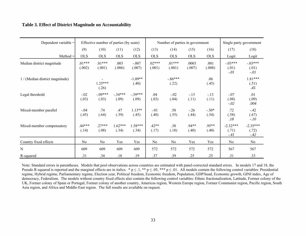
Table 3 turns to accountability, as reflected first in the fragmentation of the parliamentary

party system. The linear specification in Model 9 confirms that party system fragmentation increases

with district magnitude, although the coefficient is quite small. This suggests that, other things equal,

a jump from a median magnitude of one to ten is expected to boost the fragmentation index by one-

tenth of a unit. Adding the asymptotic term, in Model 10, confirms that there are diminishing returns

in fragmentation to increasing magnitude, although the linear magnitude term remains significant in

this specification. Legal threshold also attains significance in the asymptotic model, mitigating party

system fragmentation, as expected, while mixed-member parallel systems have no measurable

impact, and compensatory systems inflate fragmentation by a quarter of an effective party, perhaps by

encouraging localist parties in SMD competition.9 Note, however, that the improvement in fit from

the diminishing returns model of fragmentation is not as pronounced as with disproportionality or

voter-government distance: Model 10 explains just under 3 percent more of the variance in

fragmentation than does Model 9 (the R-squared changes from .31 to .34). With party system

fragmentation, again, the fixed effects results closely mirror those from the pooled models, with

evidence that higher magnitudes increase fragmentation, although with diminishing effects, legal

thresholds reduce fragmentation, and mixed-member systems increase it.

[Table 3]

Models 13 through 16 focus attention on another facet of accountability, the number of

parties holding cabinet portfolios. In the familiar sequence, Model 13 tests a linear specification

using pooled data, confirming that coalition complexity rises with median district magnitude. Adding

the asymptotic term, in Model 14, confirms some measure of diminishing returns but, as with

fragmentation, the coefficient on the linear term remains positive and significant, and the

9 Bear in mind that compensatory are, for our purposes, proportional, and we code their median magnitudes according to the proportional districts. We include a dummy for compensatory systems in our model as a check on whether adding the element of single-member district competition affects our dependent variables, even if not through the formula for translating vote shares to overall seat shares.

18

improvement in overall explanation of variance is minimal (R-squared nudges from .37 to .39). None

of the other electoral system factors has a measurable impact. The fixed-effects models, 15 and 16,

show no measurable effect of district magnitude on government coalition complexity, although the

adoption of mixed electoral systems appears to cut in opposite directions, depending whether the

reform is to parallel (simpler coalitions) or compensatory (larger coalitions) seat allocation.

Figure 4 illustrates the relationship between district magnitude and the number of parties in

government. The curve is clearly flatter (more linear) in this figure than the analogous graph for

Disproportionality. An analogous graph for Voter-government distance (not shown), like

Disproportionality, is strikingly curvilinear, whereas that for Effective number of parties (also not

shown) falls in between, somewhat more curvilinear than Parties in government, but less so than

Disproportionality or Voter-government distance. The key point is that the relationships between

district magnitude and our two dependent variables reflecting representation are distinctly curvilinear,

showing sharply diminishing returns to increases in magnitude above quite moderate levels, whereas

the relationships between district magnitude and our dependent variables reflecting accountability

exhibit more linearity.

[Figure 4]

The last panel of Table 3 shows results for the incidence of single-party government, which

some regard as the sine qua non of accountability. Models 17 and 18 estimate logit regressions on

pooled data, showing that increasing magnitude diminishes the likelihood of single-party government

and, perhaps surprisingly, that the asymptotic specification provides only modest additional leverage

beyond the pure linear one. The marginal effects on the estimated probability of single-party

government of a one-unit change in each variable, with all other variables held at their median values,

are shown in italics. The probability of single-party government falls by a percent with each unit

increase in median magnitude under both specifications.

On the whole, the results suggest that the most consistent and powerful electoral system

factor driving the representativeness-accountability trade-off is district magnitude. Various

dimensions of this trade-off, and their shapes, are shown in Figure 5, which illustrates the

19

relationships between district magnitude, on the one hand, with the predicted probabilities of good

outcomes on our two representation dependent variables and the first two of our accountability

variables. The predicted values are derived from regressions on the pooled data, with both the linear

and asymptotic district magnitude variables. We define a ‘good’ outcome as any value below the

median value in our data, insofar as we hold Disproportionality and Voter-government distance to be

representational ‘bads,’ and we regard party system fragmentation and complex government

coalitions to pose obstacles to electoral accountability. A key message from Figure 5 is that increases

in district magnitude yield diminishing returns in improving representation as well as in

compromising accountability, but the diminishing returns effect is stronger in the former than in the

latter.

[Figure 5]

The key implication of the relationships sketched in Figure 5 is that it is possible to capture

many of the representation gains of increased magnitude while sacrificing relatively less of the

accountability ideals. This point is distilled most clearly in Figure 6, which shows the combined

probability, conditional on district magnitude, of achieving good outcomes on all four of the

dependent variables from Figure 5 simultaneously. The curve rises sharply moving from pure SMDs

through the low-magnitudes, peaks in the six to eight range, and then declines.

[Figure 6]

Not surprisingly, the predicted likelihood of having better-than-median outcomes on all four

criteria is relatively low, peaking just above 10 percent. If we relax our demands, looking for good

outcomes on one representation and accountability ideal each (say, Disproportionality and Effective

number or parties, or Voter-government distance and Parties in government), then the predicted

likelihood of having one’s cake and also eating it rise to around 40 percent. Importantly, however,

the shape of the relationship between district magnitude and realization of combined representation

and accountability ideals is consistent, always rising sharply through the low magnitudes, peaking

below a median magnitude of ten, then declining as magnitude rises further.

20

This consistent relationship suggests a magnitude ‘sweet spot,’ in the four to eight range,

where the most improvements in representativeness have already been realized but where the

predicted party system fragmentation and government coalition complexity remain limited enough to

allow voters to sort our responsibility for government performance and attribute credit and blame

accordingly. The story that emerges from Figures 5 and 6 in combination is that the vast bulk of

improvements in representativeness can be realized by moving from SMDs to multi-member districts

of modest magnitudes, and that in doing so, electoral system engineers might avoid substantial

‘accountability costs’, in terms of party system fragmentation and coalition complexity, which

increase at higher magnitudes.

We acknowledge that when we pile condition upon condition – low disproportionality and

voter-government distance and fragmentation and coalition complexity – we pay a price in statistical

leverage, as the broad confidence intervals in Figure 6 testify. So, to investigate further whether we

can be confident in the relative advantages of low-magnitude districts, Figure 7 revisits our

regressions, this time substituting a series of dummy variables to capture the effects of various

magnitude intervals on the dependent variables of interest. The models use SMD systems (among

which there are 191 elections in our data) as a baseline category. We group multi-member district

systems by the magnitudes originally shown in Table 1: 2 to 3 (N=50), 4 to 6 (N=160), 7 to 10

(N=75), 11 to 20 (N=69), and greater than 20 (N=64). We chose these intervals according to a couple

of guiding principles. The intervals are smaller at the low end of the magnitude scale because we

expect the marginal effects to shift most quickly here, and because we are particularly interested in

the marginal effects in this neighborhood. We place systems with median magnitudes of two and

three into their own category because the electoral systems literature includes skepticism regarding

the dynamics of partisan competition at these particular low magnitudes (see Auth 2006 and Nohlen

2006 on magnitude 2; and Taagepera and Shugart 1989 on magnitude 3). Beyond this, we aimed for

groups with roughly similar numbers of elections to ensure comparable quality estimates across

intervals.

[Figure 7]

21

The top panel confirms that moving from SMDs to a system with a median district magnitude

in the four to six range can be expected to reduce disproportionality by almost eight points, or about

three-quarters of the total expected reduction possible by raising district magnitude. Also, the same

magnitude four to six category also achieves over eighty percent of the maximum reduction (relative

to SMDs) in voter-government distance.

The second panel shows that the four to six range yields only about half the expected increase

in party system fragmentation as the highest-magnitude systems, and less than a third the maximum

increase in expected number of parties in government (although this result is not significant in a

model with country fixed-effects).

We also ran the same models illustrated in Figure 7, but using the highest-magnitude

electoral systems (those with median district magnitude greater than 20) as the baseline category –

see Appendix C. Significance tests in these models determine whether systems in each magnitude

interval are statistically discernible from those with the highest magnitudes, rather than from SMD

systems. The key result from these specifications is that there is no measurable ‘cost,’ in terms of

disproportionality or voter-government distance, to moving from high-magnitude systems down even

as far as to those with median districts in the four to six-seat range. That is, the mid-sized districts are

either not statistically discernible – or else just barely so – from the highest-magnitude districts. On

the accountability variables, by contrast, where the high-magnitude baseline systems perform worst,

the mid-sized districts yield measurable improvement on party system fragmentation (in the pooled

model) and reduction in government coalition complexity (both models).

Conclusion: Small Multi-Member Districts Are Best

With the spread of democracy across the world in the last few decades and with more and more

established democracies tinkering with their electoral systems, we can identify the nature of the trade-

off between inclusive representation of citizens’ preferences and accountable government more

accurately than we have been able to before. With this aim in mind, our results suggest that

practitioners who seek to design an electoral system that maximizes these competing objectives are

22

best served by choosing multi-member districts of moderate magnitudes. Consistent with the

traditional view of electoral systems in political science, we find that SMD systems tend to produce a

small number of parties and single-party government, but also have relatively unrepresentative

parliaments. On the other side, electoral systems with large multi-member districts have highly

representative parliaments, but also have highly fragmented party systems and unwieldy multi-party

coalition governments. In contrast, electoral systems with small multi-member districts – with

median magnitude between four and eight seats, for example – tend to have highly representative

parliaments and a moderate number of parties in parliament and in government.

On the representation side, our results suggest that increasing the district size from one to

around five reduces the disproportionality of representation a parliament by three-quarters and

reduces the ideological distance between the median citizen and the median government party even

more sharply. This is a result of both the greater opportunities for medium-sized parties to win seats

and the new incentives for supporters of small parties, who may simply prefer to ‘throw away’ their

votes under SMD elections, to coordinate into medium-sized parties. Increasing the district

magnitude beyond six does not improve representation much further. On the accountability side,

meanwhile, increasing the district size from one to around five increases the number of effective

parties in parliament by around one, and increases the number of parties in government by about a

half. Countries with small multi-member districts are more likely to have coalition governments than

countries with SMDs but these coalitions are likely to be between two or a maximum of three parties.

Put another way, low-magnitude PR simultaneously fosters inclusiveness and limits the political

unruliness high magnitudes invite via party system fragmentation and coalition complexity.

In closing, is also worth noting other research that points to an advantage of low-magnitude

districts for the accountability of individual legislators. Carey (2009) describes a trend in electoral

reform toward systems that allow voters to cast preference votes for individual candidates, and notes

that voters overwhelmingly choose to exercise the preference vote when given the option. Yet, the

promise open list elections hold of individual accountability is conditional on limited district

magnitude. In high-magnitude elections, open list systems confront voters with a bewildering array

23

of candidates (Samuels 1999), whereas low magnitudes curb both party system fragmentation,

keeping a lid on the number of lists, and the number of candidates per list. As a result, voters under

low-magnitude, open-list systems are better able than those in other systems to identify and hold their

representatives accountable. Chang and Golden (2007), for example, find that corruption is lower in

countries with open-list than with closed-list proportional representation, provided that average

district magnitude is below 10, whereas at very high magnitudes (above 20) open-lists systems are

associated with more corruption. Hence, low magnitudes make it possible to combine candidate

preference votes and individual accountability with proportionality and partisan inclusiveness.

In short, legislative elections work best when they offer opportunities for multiple winners,

and thus afford voters an array of viable options, but at the same time do not encourage niche parties

or overwhelm voters with a bewildering menu of alternatives. The evidence from a wide range of

indicators all point toward low-magnitude proportional representation as providing a good balance

between the ideals of representation and accountability.

24

References

Acemoglu, Daron, Simon Johnson and James A. Robinson (2001) ‘The Colonial Origins of Comparative Development: An Empirical Investigation’, American Economic Review 91: 1369-1401.

Adserà, Alícia, Carles Boix, and Mark Payne (2003) ‘Are You Being Served? Political Accountability and Quality of Government’, The Journal of Law, Economics, and Organization 19(2): 445-490.

Auth, Pepe (2006) ‘De un sistema proporcional excluyente a uno icluyente’, Mimeo. Santiago: Fundacion Chile: 1-21.

Benoit, Kenneth (2007) ‘Electoral Laws as Political Consequences: Explaining the Origins and Change of Electoral Institutions’, Annual Review of Political Science 10: 363-390.

Benoit, Kenneth and John W. Schiemann (2001) ‘Institutional Choice in New Democracies: Bargaining over Hungary’s 1989 Electoral Law’, Journal of Theoretical Politics 13(2): 153-182.

Birch, Sarah (2001) Electoral Systems and Political Transformation in Post-Communist Europe, London: Palgrave.

Boix, Carles (1999) ‘Setting the Rules of the Game: The Choice of Electoral Systems in Advanced Democracies’, American Political Science Review 93(3): 609-624.

Boix, Carles (2003) Democracy and Redistribution, Cambridge: Cambridge University Press.

Carey, John M. (2009) Legislative Voting and Democratic Accountability, Cambridge: Cambridge University Press.

Center on Democratic Performance (2006) Election Results Archive, Binghamton University Department of Political Science, www.binghamton.edu/cdp/era. Accessed 22 December 2006.

Chang, Eric C.C. and Miriam Golden (2007) ‘Electoral Systems, District Magnitude and Corruption’, British Journal of Political Science 37: 115-137.

Cheibub, José Antonio (2006a) Presidentialism, Parliamentarism, and Democracy, Cambridge: Cambridge University Press.

Cheibub, José Antonio (2006b) ‘Presidentialism, Electoral Identifiability, and Budget Balances in Democratic Systems’, American Political Science Review 100(3): 335-350.

Colomer, Josep (2005) ‘It’s Parties That Choose Electoral Systems (or, Duverger’s Law Upside Down)’, Political Studies 53: 1-21.

Cox, Gary (1997) Making Votes Count: Strategic Coordination in the World’s Electoral Systems, Cambridge: Cambridge University Press.

Culver, William W. and Alfonso Ferrufino (2000) ‘Diputados Uninominales: La Participacion Politica En Bolivia’, Contribuciones 1: 1-28.

Deininger, Klaus W (2006) ‘Measuring Income Inequality Database’, World Bank, http://econ.worldbank.org/WBSITE/EXTERNAL/EXTDEC/EXTRESEARCH/0,,contentMDK:20699070~pagePK:64214825~piPK:64214943~theSitePK:469382,00.html. Accessed 22 December 2006.

Fearon, James D. (2003) ‘Ethnic and Cultural Diversity by Country’, Journal of Economic Growth 8: 195-222.

25

Gallagher, Michael (1991) ‘Proportionality, Disproportionality and Electoral Systems’, Electoral Studies 10: 33-51.

Gallagher, Michael (2007) Electoral Systems Web Site, Dublin: Trinity College. http://www.tcd.ie/Political_Science/Staff/Michael.Gallagher/ElSystems/index.php.

Golder, Matt (2005) ‘Democratic Electoral Systems Around the World, 1946-2000’, Electoral Studies 24(1): 103-121.

Grofman, Bernard N. and Arend Lijphart (eds.) (1986) Electoral Laws and Their Political Consequences, New York: Agathon Press.

Hellwig, Timothy and David Samuels (2007) ‘Electoral Accountability and the Variety of Democratic Regimes’, British Journal of Political Science 38: 65-90.

Huber, John D. (2007) Government CompositionDataset, Columbia University.

Huber, John D. and G. Bingham Powell (1994) ‘Congruence Between Citizens and Policymakers in Two Visions of Democracy’, World Politics 46: 291-326.

Jacobs, Alan M. (2009) ‘How Do Ideas Matter? Mental Models and Attention in German Pension Politics’, Comparative Political Studies 42(2):252-279.

Keesing's Record of World Events, London: Longman.

Kim, HeeMin, G. Bingham Powell, Jr. and Richard C. Fording (2009) ‘Electoral Systems, Party Systems, and Ideological Representation: An Analysis of Distortion in Western Democracies’, Comparative Politics, forthcoming.

Laakso, Markku, and Rein Taagepera (1979) ‘Effective Number of Parties: A Measure with Application to West Europe’, Comparative Political Studies 12: 3-27.

Lijphart, Arend (1984) Democracies: Patterns of Majoritarian and Consensus Government in Twenty-One Countries, New Haven, CT: Yale University Press.

Lijphart, Arend (1994) Electoral systems and Party Systems: A Study of Twenty-Seven Democracies, 1945-1990, Oxford: Oxford University Press.

Lijphart, Arend (2004) ‘Constitutional Design for Divided Societies’, Journal of Democracy 15(2): 96-109.

Maddison, Angus (2007) World Population, GDP and Per Capita GDP, 1-2003 AD, http://www.ggdc.net/maddison/Historical_Statistics/horizontal-file_03-2007.xls.

Mainwaring, Scott (1991) ‘Politicians, Electoral Systems, and Parties: Brazil in Comparative Perspective’, Comparative Politics 24(1): 21-43.

McKean, Margaret; Scheiner, Ethan (2000) ‘Japan’s New Electoral System: Plus la change’, Electoral Studies 19(4): 447-477.

Miller, George A. 1956. “The magical number seven, plus or minus two: Some limits on our capacity for processing information.” Psychological Review 63:81-97.

Monroe, Burt L. and Amanda G. Rose (2002) ‘Electoral Systems and Unimagined Consequences: Partisan Effects of Districted Proportional Representation’, American Journal of Political Science 46(1): 67-89.

Moser, Robert G. (1999) ‘Electoral Laws and the Number of Parties in Postcommunist States’, World Politics 51(3): 359-384.

Nohlen, Dieter (2005) Elections in the Americas: A Data Handbook, Oxford: Oxford University Press.

26

Nohlen, Dieter (2006) ‘La reforma del sistema binominal desde una perspective comparada’, Revista de Ciencia Politica 26(1): 191-202.

Nohlen, Dieter, Michael Krennerich and Bernhard Thibaut (1999) Elections in Africa: A Data Handbook, Oxford: Oxford University Press.

Norris, Pippa (2005) Democracy Indicators Cross-national Time-Series Dataset Release 1.0. John F. Kennedy School of Government at Harvard, http://ksghome.harvard.edu/~pnorris/Data/Data.htm. Accessed 24 September 2006.

Nunley, Albert C (2007) African Elections Database, http://africanelections.tripod.com. Accessed 24 May 2007.

Persson, Torsten and Guido Tabellini (2003) The Economic Effects of Constitutions, Cambridge, MA: MIT Press.

Plümper, Thomas and Vera E.Troeger (2007) ‘Efficient Estimation of Time-Invariant and Rarely Changing Variables in Finite Sample Panel Analyses With Unit Fixed Effects’, Political Analysis 15: 124-139.

Powell, G. Bingham (2000) Elections as Instruments of Democracy, New Haven, CT: Yale University Press.

Powell, G.B. and Georg Vanberg (2000) ‘Election Laws, Disproportionality and Median Correspondence: Implications for Two Visions of Democracy’, British Journal of Political Science 30(3): 383-411.

Przeworski, Adam, Michael Alvarez, José Antonio Cheibub and Fernando Limongi (2000) Democracy and Development, Cambridge: Cambridge University Press.

Przeworski, Adam, José Antonio Cheibub and Sebastion Saiegh (2004) ‘Government Coalitions and Legislative Success Under Presidentialism and Parliamentarism’, British Journal of Political Science 34: 565-587.

Rachadell, Manuel (1991) ‘El Sistema Electoral y La Reforma De Los Partidos’, in Carlos Blanco and Edgar Paredes Pisani (eds) Venezuela, democracia y futuro: Los partidos politicos en la decada de los 90. Reflexiones para un cambio neceario, Caracas, Venezuela: Comision Presidencial para la Reforma del Estado, 203-210.

Reynolds, Andrew, Ben Reilly, and Andrew Ellis (2005) Electoral System Design: The New International IDEA Handbook, Stockholm: International IDEA.

Rokkan, Stein (1970) Citzens, Elections, Parties, Oslo: Universitetsforlaget.

Samuels, David J. (1999) ‘Incentives to Cultivate a Party Vote in Candidate-Centered Electoral Systems’, Comparative Political Studies 32(4): 487-518.

Shugart, Matthew S. and Martin P. Wattenberg (eds) (2001) Mixed-Member States: The Best of Both Worlds? Oxford: Oxford University Press.

Sinopoli, Francesco De and Giovanna Iannantuoni (2001) ‘A Spatial Voting Model where Proportional Rule Leads to Two-Party Equilibria’, Wallis Institute of Political Economy, www.wallis.rochester.edu/conference08/SPARES.pdf.

Strom, Kaare (1990) Minority Government and Majority Rule, Cambridge: Cambridge University Press.

Taagepera, Rein (2007) Predicting Party Sizes: The Logic of Simple Electoral Systems, Oxford: Oxford University Press.

Taagepera, Rein and Matthew Shugart (1989) Seats and Votes: The Effects and Determinants of Electoral Systems, New Haven, CT: Yale University Press.

27

Tomz, Michael and Robert P. Van Houweling. 2008. “Candidate positioning and voter choice.” American Political Science Review 102(3):303-318.

Tsebelis, George (2002) Veto Players: How Political Institutions Work, Princeton, NJ: Princeton University Press.

United Nations University-World Institute for Development Economics Research (2005) World Income Inequality Database, V 2.0b, http://www.wider.unu.edu/wiid/wiid.htm. Accessed May 15, 2007.

28

Figure 1. Two Versions of the Trade-Off Between Accountability and Representation in the Design of Electoral Systems

Representation

Acc

ount

abili

ty

Single-member districts (e.g. Australia, India, UK)

Pure PR (High-magnitude multi-member districts)(e.g. Israel, Netherlands, South Africa)

Low-magnitude multi-member districts (e.g. Costa Rica, Mali, Spain)

?

29

Table 1. Electoral Systems in Modern Democracies, Grouped by Median District Magnitude

Median DM = 1 2 to 3 4 to 6 7 to 10 11 to 20 Greater than 20 Australia Argentina (~1983) √ Austria (1949, 1962-1970) Argentina (1983) √ Austria (1971-) √ Czech Rep. (-1998) √ Bangladesh Chile Belgium (~1965) Austria (1953-1959) √ Benin (1991) Germany (-1953) √ Botswana Dominican Republic (1994-) Benin (1995-) Belgium (1965) Bolivia (-1989) Israel √ Bulgaria (1990) Ecuador (-1996) Bolivia (1993-) Brazil Croatia †√ Italy (-1992) √ Canada El Salvador (1997-) Colombia (1970-) Bulgaria (1991-) √ Czech Republic (2002-) √ Lesotho France (except 1986) Ireland (1969-1977) Costa Rica (1978-) Colombia (1960-1966) Czechoslovakia √ Mexico √ India Mali Denmark (-1968) Costa Rica (1958-1974) Finland Moldova √ Italy (1994-2001) †√ Mauritius Dominican Rep. (1978-90) Cyprus √ Germany (1957-) √ Namibia Jamaica Mongolia (1992) Ecuador (1998) Denmark (1971-) √ Latvia √ Netherlands √ Japan (1996-) † Nicaragua (1995-) El Salvador (-1994) Estonia √ Macedonia (2002) New Zealand (1996-) Lithuania †√ Panama (1989) France (1946-1956) Honduras (1993-) Mozambique √ Slovakia √ Macedonia (-1998) Paraguay France (1986) √ Indonesia √ Poland (1991) South Africa Madagascar † Peru (2001-) Greece √ Nicaragua (1990) Poland (2001-) √ Uruguay Malawi Thailand (1992-1996) Guatemala Norway (1953-) Sweden (1970-) √ Mongolia (1996-) Venezuela (1993-) Guyana (1992-1997) Peru (1980) Switzerland (-1963) √ Nepal Honduras (1989) Poland (1993-1997) √ New Zealand (-1993) Hungary √ Romania Panama (1994-) †√ Ireland (-1965, 1981-) Sri Lanka (2001-) Papua New Guinea Japan (-1993) Sweden (-1968) √ Philippines (-1993) Norway (1949) Taiwan †√ Philippines (1998-) †√ Peru (1985-1990) Russia †√ Portugal Sri Lanka (-1977) Serbia & Montenegro South Korea † Spain √ Thailand (2001) †√ Switzerland (1967-1999) √ Trinidad & Tobago Turkey √ Ukraine Venezuela (-1998) United Kingdom United States Note: † indicates a mixed-member parallel system. √ indicates a legal threshold for representation.

30

Figure 2. Trade-Off Between Disproportionality of Representation and Party System Fragmentation

02

46

810

Effe

ctiv

e N

umbe

r of P

artie

s-by

sea

ts

0 10 20 30 40Disproportionality

Note: Blue = system with single-member districts, Green = system with a median district magnitude between 2 and 10. Red = system with a median district magnitude greater than 10.

31

Table 2. Effect of District Magnitude on Representation

Dependent variable = Disproportionality Voter-government distance

(1) (2) (3) (4) (5) (6) (7) (8)

Median district magnitude -.05*** (.004)

-.01** (.003)

-.10*** (.03)

-.02 (.03)

-.01 (.02)

.02 (.02)

-.09 (.08)

.01 (.10)

1 / (Median district magnitude) 10.05*** (.96)

8.40*** (1.72)

15.08*** (3.04)

14.14* (8.11)

Legal threshold -.26 (.17)

.37*** (.12)

-.48 (.41)

-.14 (.41)

-1.27** (.55)

.02 (.66)

-3.15* (1.69)

-1.14 (2.04)

Mixed-member parallel 3.63** (1.36)

-2.69** (1.31)

3.22** (1.68)

-.90 (1.96)

3.48 (3.00)

-9.15** (3.69)

-.14 (5.73)

-14.31 (9.93)

Mixed-member compensatory -.57 (.82)

.76 (.64)

-1.99*** (1.51)

-1.69 (1.48)

-3.57* (2.05)

2.70 (2.37)

3.34 (5.12)

9.21 (6.12)

Country fixed effects No No Yes Yes No No Yes Yes

N 609 609 609 609 310 310 314 314

R-squared .43 .56 .12 .16 .14 .19 .08 .09 Note: Method: OLS regression. Standard errors in parentheses. Models that pool observations across countries are estimated with panel-corrected standard errors. * p ≤ .1, ** p ≤ .05, *** p ≤ .01. All models contain the following control variables: Presidential regime, Hybrid regime, Parliamentary regime, Election year, Political freedom, Economic freedom, Population, GDP/head, Economic growth, GINI index, Age of democracy, Federalism. The models without country fixed effects also contain the following control variables: Ethnic fractionalization, Latitude, Former colony of the UK, Former colony of Spain or Portugal, Former colony of another country, Americas region, Western Europe region, Former Communist region, Pacific region, South Asia region, and Africa and Middle-East region. The full results are available on request.

32

Figure 3. Estimation of the Effect of District Magnitude on Disproportionality

05

1015

2025

Pred

icte

d D

ispr

opor

tiona

lity

0 5 10 15 20Median District Magnitude

Note: The line is a bivariate asymptotic regression model, with 95 percent confidence intervals shaded, using the predicted values for disproportionality from Model 2 in Table 2 for electoral systems with a median district magnitude of less than 30.

33

Table 3. Effect of District Magnitude on Accountability

Dependent variable = Effective number of parties (by seats) Number of parties in government Single party government

(9) (10) (11) (12) (13) (14) (15) (16) (17) (18)

Method = OLS OLS OLS OLS OLS OLS OLS OLS Logit Logit

Median district magnitude .01*** (.002)

.01*** (.001)

.003 (.006)

-.007 (.007)

.02*** (.001)

.01*** (.001)

.0003 (.007)

.001 (.008)

-.03*** (.01) -.01

-.03*** (.01) -.01

1 / (Median district magnitude) -1.25***

(.26)

-1.09**(.40)

-.86*** (.22)

.06 (.45)

1.81*** (.51) .45

Legal threshold -.02 (.03)

-.09***(.03)

-.34***(.09)

-.39***(.09)

.04 (.03)

-.02 (.04)

-.13 (.11)

-.13 (.11)

-.07 (.08) -.02

.01 (.09) .004

Mixed-member parallel -.04 (.45)

.74 (.64)

.47 (.39)

1.13**(.45)

-.01 (.40)

.58 (.55)

-.26 (.44)

-.30* (.54)

.72 (.58) .18

-.42 (.67) -.10

Mixed-member compensatory .44*** (.14)

.27*** (.08)

1.62***(.34)

1.58***(.34)

.42** (.17)

.30 (.18)

.94** (.40)

.95** (.40)

-2.32*** (.71) -.41

-2.35*** (.72) -.42

Country fixed effects No No Yes Yes No No Yes Yes No No

N 609 609 609 609 572 572 572 572 567 567

R-squared .31 .34 .18 .19 .37 .39 .25 .25 .31 .33 Note: Standard errors in parentheses. Models that pool observations across countries are estimated with panel-corrected standard errors. In models 17 and 18, the Pseudo R-squared is reported and the marginal effects are in italics. * p ≤ .1, ** p ≤ .05, *** p ≤ .01. All models contain the following control variables: Presidential regime, Hybrid regime, Parliamentary regime, Election year, Political freedom, Economic freedom, Population, GDP/head, Economic growth, GINI index, Age of democracy, Federalism. The models without country fixed effects also contain the following control variables: Ethnic fractionalization, Latitude, Former colony of the UK, Former colony of Spain or Portugal, Former colony of another country, Americas region, Western Europe region, Former Communist region, Pacific region, South Asia region, and Africa and Middle-East region. The full results are available on request.

34

Figure 4. Estimation of the Effect of District Magnitude on the Number of Parties in Government

01

23

45

Pre

dict

ed N

o. o

f Par

ties

in G

ovt.

0 5 10 15 20Median District Magnitude

Note: The line is a bivariate asymptotic regression model, with 95 percent confidence intervals shaded, using the predicted values for the number of parties in government from Model 14 in Table 3 for electoral systems with a median district magnitude of less than 30.

35

Figure 5. District Magnitude and the Probability of Favorable Outcomes

0.2

.4.6

.8P

roba

bilit

y

0 5 10 15 20 25Median District Magnitude

Note: The figure plots the predicted probabilities that an election produced a favorable outcome in the relevant variable, fitting an asymptotic model to the predicted values, with 95 percent confidence intervals shaded.

Disproportionality< 5

Effective no. of parties < 3

Parties in government ≤ 2

Voter-government distance < 5

36

Figure 6. District Magnitude and the Probability of Combined Favorable Outcomes

0.0

5.1

.15

Pro

babi

lity

0 5 10 15 20 25Median District Magnitude

Note: The figures plots the predicted probability that an election produced a favorable outcome in all four of our measures: a disproportionality score less than 5; a voter-government distance score less than 5; less than 3 effective number of parliamentary parties; and 2 or less parties in government. The 95% (the outer area) and 50% (inner area) confidence intervals are shaded.

37

Figure 7. The Effect of District Magnitude Thresholds

Note: These figures plot the coefficients and standard errors from a series of regression. The baselines in the model are the outcome of elections with single-member districts. The models that pool observations across countries are estimated with panel-corrected standard errors. See the note to Table 2 for the list of control variables which are included but not reported here. The full results are available on request.

Median district magnitude >20

Median district magnitude 11 to 20

Median district magnitude 7 to 10

Median district magnitude 4 to 6

Median district magnitude 2 to 3

-12 -10 -8 -6 -4 -2 0 -30 -20 -10 0 10

Voter-government distance DisproportionalityDependent variable =

Country fixed effects models Pooled models

Median district magnitude >20

Median district magnitude 11 to 20

Median district magnitude 7 to 10

Median district magnitude 4 to 6

Median district magnitude 2 to 3

0 .5 1 1.5 2 -1 0 1 2 3

No. of parties in government Effective no. of parties Dependent variable =

38

Appendix A. Descriptive Statistics

Obs Mean Median Std.Dev. Minimum Maximum

Dependent Variables Disproportionality 609 7.10 5.07 6.25 .28 34.52 Voter-government distance 314 8.44 5.90 8.32 0 46.43 Effective number of parties (by seats) 609 3.36 2.96 1.50 1 10.87 Parties in government 572 2.06 2 1.49 1 14 Single party government 566 .49 0 .50 0 1 Electoral System Variables

Median district magnitude 609 14.22 5 31.51 1 150 1/(Median district magnitude) 609 .42 .20 .40 .01 1 Legal threshold 609 1.29 0 2.00 0 10 Mixed-member parallel 609 .04 0 .20 0 1 Mixed-member compensatory 609 .05 0 .22 0 1 Note: Full results of all models presented in paper, plus robustness checks, are available from the authors.

39

Appendix B. Coding of the Variables and Sources

Age of democracy.Measured as election year minus the year in which the country first scored +6 or above on the Polity IV index, plus 1 (i.e. first year a country is democratic = 1). Disproportionality.Disproportionality index (Gallagher formula). Source: Gallagher (2007), except Latin American elections calculated from data in Nohlen (2005); certain African countries (Benin, Bostwana, Ghana, Lesotho, Madagascar, Malawi, Mali, Mauritius, Mozambique and Namibia) calculated from data in Nunley (2004), and others (Benin, Botswana, Malawi, Mali, and Mauritius) calculated from data in Nohlen, Krennerich and Thibaut (1999). Economic freedom.Freedom House score. Data for early elections entered at value of earliest datapoint. Source: most values from Norris (2005). Economic growth. Mean three-year GDP growth (two years prior to election year + election year). Source: Maddison (2007), except for Cyprus, from Groningen Growth and Development Centre data, http://www.ggdc.net, and Guyana and Papua New Guinea, from Cheibub (2006b). One missing value (Israel 1949) entered as the mean value of the variable. Effective number of parties (by seats). Effective number of (legislative) parties in the election, according to lower chamber seat shares. Source: Golder (2005); Gallagher (2007). Effective number of parties (by votes). Effective number of (electoral) parties in the election, according to vote shares. Source: Golder (2005); Gallagher (2007). Election year.Year of election. Source: Golder (2005); various web-based sources. Ethnic fractionalization.Ethnic fractionalization index according to Fearon (2003). The index includes ethnic, linguistic and religious groups, using data from CIA World Factbook, the Encyclopedia Britannica, relevant Library of Congress Country Studies, the Minorities at Risk dataset, national censuses, and various other sources. Fearon’s data is from 1990 to 1995, but his numbers are constant values for this period. We have entered the same value for all elections in each country, which means that our coding of this variable only varies across countries and does not vary within countries. Two missing values (for Serbia and Montenegro and Taiwan) were entered as the mean value of this variable. Federalism.1 = country has a federal political structure, 0 = other. Source: Adserà, Boix and Paine (2003). Former colony of another country.1 = former colony of a country other than UK, Spain or Portugal, 0 = other. Former colony of Spain or Portugal.1 = former colony of Spain or Portugal, 0 = other. Former colony of the UK.1 = former colony of United Kingdom, 0 = other. Source: Persson and Tabellini (2003). GDP/head.GDP per capita, 1990 International Geary-Khamis dollars, divided by 1000. Source: Maddison (2007), except for Cyprus, from Groningen Growth and Development Centre data, http://www.ggdc.net, and Guyana and Papua New Guinea, from Norris (2005). GINI index.Gini index of economic inequality. Source: Deininger (2006); United Nations University-World Institute for Development Economics Research (2005). Data imputed for missing values from nearest year where data are available. Latitude.Latitude of the capital city of a country (ranging from 90˚S to 90˚N), rescaled between 0 (90˚S) and 1 (90˚N). I.e. a measure of how far north a country is. Source: http://www.mapsofworld.com/utilities/world-latitude-longitude.htm. Legal threshold.National-level legal threshold. Source: Center on Democratic Performance (2006), Mainwaring (1991). Median district magnitude.Median district magnitude in the election. This means the magnitude (M) of the district for which there are an equal number of districts with greater, and lesser, values on M. We measure the median district magnitude as follows: in non mixed-member systems, M is the magnitude of the district with an equal number of larger and smaller districts; in compensatory mixed-member system, M is the median size of the PR districts; and in mixed-member parallel systems, M is the median size of all districts. Source: Golder (2005); Center on Democratic Performance (2006); Reynolds, Reilly and Ellis (2005); Benoit and Schiemann (2001).

40

Median district magnitude 1.1 = median district magnitude of 1, 0 = other. Median district magnitude 2 to 3.1 = median district magnitude of between 2 and 3 (inclusive), 0 = other. Median district magnitude 4 to 6. 1 = median district magnitude of between 4 and 6 (inclusive), 0 = other. Median district magnitude 7 to 10. 1 = median district magnitude of between 7 and 10 (inclusive), 0 = other. Median district magnitude 11 to 20. 1 = median district magnitude of between 11 and 20 (inclusive), 0 = other. Median district magnitude >20. 1 = median district magnitude of more than 20, 0 = other. Source: Golder (2005); Center on Democratic Performance (2006); Reynolds, Reilly and Ellis (2005); Benoit and Schiemann (2001). Mixed-member parallel. 1 = a mixed-member (single-member district plus multi-member district) system in which seats in the multi-member tier are not allocated to compensate for disproportionalities in the single-member tier, 0 = other. Mixed-member compensatory. 1 = a mixed-member (single-member district plus multi-member district) system in which seats in the multi-member tier are allocated to compensate for disproportionalities in the single-member tier, 0 = other. Sources: Golder (2005); Birch (2001). No. of parties in government. Variable denotes the total number of parties holding cabinet portfolios in first government formed after election. Source: Huber (2007) for Australia, Austria, Belgium, Canada, Denmark, Finland, France, Germany, Ireland, Italy, Netherlands, New Zealand, Norway, Portugal, Spain, Sweden, United Kingdom. Data for all other cases calculated from information in Keesing's Record of World Events. Political freedom. Political freedom score from Polity IV. Source: most values from Norris (2005). Population. Population of a country in the year of the election, divided by 1 million. Source: UN Population Division annual estimates. Where data is missing, the estimated population for the nearest year is entered. Regime-Hybrid. 1 = hybrid (parliamentary-presidential, semi-presidential) system, 0 = other. Regime-Parliamentary. 1 = parliamentary system, 0 = other. Regime-Presidential. 1 = presidential system, 0 = other. Source: Cheibub (2006a), except for Switzerland, which we code as Hybrid. Region-Africa and Middle-East. 1 = Benin, Botswana, Ghana, Israel, Lesotho, Madagascar, Malawi, Mali,. Mozambique, Namibia, South Africa, Turkey, 0 = other. Region-Americas. 1 = Argentina, Bolivia, Brazil, Canada, Chile, Colombia, Costa Rica, Dominican Republic, Ecuador, El Salvador, Guatemala, Guyana, Honduras, Jamaica, Nicaragua, Panama, Paraguay, Peru, Trinidad & Tobago, USA, Uruguay, Venezuela, 0 = other. Region-Former Communist. 1 = Albania, Armenia, Bulgaria, Croatia, Czech Republic, Czechoslovakia, Hungary, Latvia, Lithuania, Macedonia, Moldova, Poland, Romania, Russia, Serbia and Montenegro, Slovakia, Ukraine, 0 = other. Region-Pacific. 1 = Australia, Fiji, Japan, New Zealand, Papua New Guinea, Philippines, South Korea, Taiwan, 0 = other. Region-South Asia.1 = Bangladesh, India, Indonesia, Mauritius, Mongolia, Nepal, Sri Lanka, Thailand, 0 = other. Region-Western Europe.1 = Austria, Belgium, Cyprus, Denmark, Estonia, Finland, France, Germany, Greece, Ireland, Italy, Netherlands, Norway, Portugal, Spain, Sweden, Switzerland, United Kingdom, 0 = other Voter government distance.Voter-government distance, based on location of median voter and median member of government, as calculated by HeeMin Kim and Richard Fording. The data for the US are dropped, so that only data for parliamentary systems are entered. For minority governments, we use difference between the location of the median voter and the median member of parliament. Source: Kim, Powell and Fording (2009).

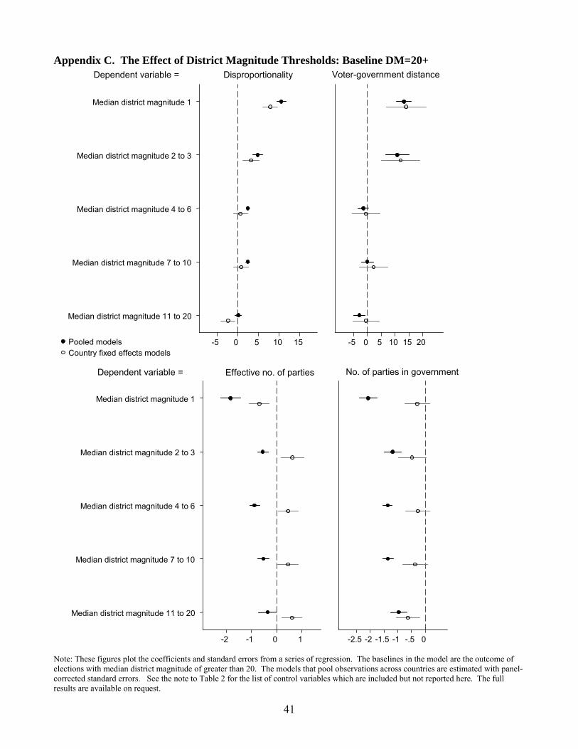
41

Appendix C. The Effect of District Magnitude Thresholds: Baseline DM=20+ Note: These figures plot the coefficients and standard errors from a series of regression. The baselines in the model are the outcome of elections with median district magnitude of greater than 20. The models that pool observations across countries are estimated with panel-corrected standard errors. See the note to Table 2 for the list of control variables which are included but not reported here. The full results are available on request.

Median district magnitude 11 to 20

Median district magnitude 7 to 10

Median district magnitude 4 to 6

Median district magnitude 2 to 3

Median district magnitude 1

-5 0 5 10 15 -5 0 5 10 15 20 Country fixed effects models Pooled models

Voter-government distance DisproportionalityDependent variable =

Median district magnitude 11 to 20

Median district magnitude 7 to 10

Median district magnitude 4 to 6

Median district magnitude 2 to 3

Median district magnitude 1

-2 -1 0 1 -2.5 -2 -1.5 -1 -.5 0

No. of parties in government Effective no. of parties Dependent variable =