The efficient solution of the (quietly constrained) noisy, linear regulator problem
16
J. Math. Anal. Appl. 333 (2007) 823–838 www.elsevier.com/locate/jmaa The efficient solution of the (quietly constrained) noisy, linear regulator problem John Gregory ∗ , H.R. Hughes Department of Mathematics, Southern Illinois University Carbondale, Carbondale, IL 62901-4408, USA Received 13 January 2006 Available online 8 January 2007 Submitted by L. Chen Abstract In a previous paper we gave a new, natural extension of the calculus of variations/optimal control theory to a (strong) stochastic setting. We now extend the theory of this most fundamental chapter of optimal control in several directions. Most importantly we present a new method of stochastic control, adding Brownian mo- tion which makes the problem “noisy.” Secondly, we show how to obtain efficient solutions: direct stochastic integration for simpler problems and/or efficient and accurate numerical methods with a global a priori error of O(h 3/2 ) for more complex problems. Finally, we include “quiet” constraints, i.e. deterministic re- lationships between the state and control variables. Our theory and results can be immediately restricted to the non “noisy” (deterministic) case yielding efficient, numerical solution techniques and an a priori error of O(h 2 ). In this event we obtain the most efficient method of solving the (constrained) classical Linear Regulator Problem. Our methods are different from the standard theory of stochastic control. In some cases the solutions coincide or at least are closely related. However, our methods have many advantages including those mentioned above. In addition, our methods more directly follow the motivation and theory of classical (deterministic) optimization which is perhaps the most important area of physical and engineering science. Our results follow from related ideas in the deterministic theory. Thus, our approximation methods follow by guessing at an algorithm, but the proof of global convergence uses stochastic techniques because our tra- jectories are not differentiable. Along these lines, a general drift term in the trajectory equation is properly viewed as an added constraint and extends ideas given in the deterministic case by the first author. © 2006 Elsevier Inc. All rights reserved. Keywords: Stochastic optimal control; Linear regulator problem; Constrained optimal control; Optimal control; Stochastic * Corresponding author. E-mail addresses: [email protected] (J. Gregory), [email protected] (H.R. Hughes). 0022-247X/$ – see front matter © 2006 Elsevier Inc. All rights reserved. doi:10.1016/j.jmaa.2006.11.032
-
Upload
john-gregory -
Category
Documents
-
view
213 -
download
0
Transcript of The efficient solution of the (quietly constrained) noisy, linear regulator problem

J. Math. Anal. Appl. 333 (2007) 823–838
www.elsevier.com/locate/jmaa
The efficient solution of the (quietly constrained) noisy,linear regulator problem
John Gregory ∗, H.R. Hughes
Department of Mathematics, Southern Illinois University Carbondale, Carbondale, IL 62901-4408, USA
Received 13 January 2006
Available online 8 January 2007
Submitted by L. Chen
Abstract
In a previous paper we gave a new, natural extension of the calculus of variations/optimal control theory toa (strong) stochastic setting. We now extend the theory of this most fundamental chapter of optimal controlin several directions. Most importantly we present a new method of stochastic control, adding Brownian mo-tion which makes the problem “noisy.” Secondly, we show how to obtain efficient solutions: direct stochasticintegration for simpler problems and/or efficient and accurate numerical methods with a global a priorierror of O(h3/2) for more complex problems. Finally, we include “quiet” constraints, i.e. deterministic re-lationships between the state and control variables. Our theory and results can be immediately restricted tothe non “noisy” (deterministic) case yielding efficient, numerical solution techniques and an a priori errorof O(h2). In this event we obtain the most efficient method of solving the (constrained) classical LinearRegulator Problem. Our methods are different from the standard theory of stochastic control. In some casesthe solutions coincide or at least are closely related. However, our methods have many advantages includingthose mentioned above. In addition, our methods more directly follow the motivation and theory of classical(deterministic) optimization which is perhaps the most important area of physical and engineering science.Our results follow from related ideas in the deterministic theory. Thus, our approximation methods followby guessing at an algorithm, but the proof of global convergence uses stochastic techniques because our tra-jectories are not differentiable. Along these lines, a general drift term in the trajectory equation is properlyviewed as an added constraint and extends ideas given in the deterministic case by the first author.© 2006 Elsevier Inc. All rights reserved.
Keywords: Stochastic optimal control; Linear regulator problem; Constrained optimal control; Optimal control;Stochastic
* Corresponding author.E-mail addresses: [email protected] (J. Gregory), [email protected] (H.R. Hughes).
0022-247X/$ – see front matter © 2006 Elsevier Inc. All rights reserved.doi:10.1016/j.jmaa.2006.11.032

824 J. Gregory, H.R. Hughes / J. Math. Anal. Appl. 333 (2007) 823–838
1. Introduction
One of the most interesting subject areas in control theory is the Linear Regulator Problem:
min J (x) =b∫
a
[uT (t)R(t)u(t) + xT (t)P (t)x(t)
]dt + xT
b Kxb,
s.t. x′(t) = A(t)x(t) + B(t)u(t), x(a) = xa, (1.1)
where x is n-dimensional, u is m-dimensional, the matrices are in C1[a, b], R is positive definite,P is positive semidefinite, and T denotes transpose. The interested reader may find this materialin [9–11].
Many problems in a variety of disciplines can be formulated as moving on the given trajectorywith J (x) the cost functional or error. This problem is of deep interest in a variety of applicationsbecause of its practical importance and relative ease of numerical solution. An additional bonusis the fact that this problem, using feedback control, yields a formal solution [10]. The numericalalgorithms in [5] or [6] yield solutions of the Linear Regulator Problem with an a priori errorof O(h2). Moreover, these numerical methods can be applied to “nonlinear” problems usingiteration methods which converge in one step regardless of the initial guess, also with an a priorierror of O(h2).
About 15 years ago, the first author looked for ways to generalize this type of problem(see [5]). Continuity conditions were weakened, multipliers were used in an unusual way toturn this (and more general constrained problems) into problems in the calculus of variations andefficient and accurate numerical methods were developed to solve general problems where theintegrand in J was the general function f (t, x,u). Thus, for the first time, simpler problems inthe calculus of variations/optimal control theory could be solved using the Euler equations withappropriate boundary conditions while more difficult problems could be efficiently calculatedwith an a priori error of O(h2), where h was the node size.
Recently, the authors have developed a new variational theory of stochastic control (see [3]).Of interest is that our ideas are modifications of the basic development in the calculus ofvariations to deal with “noise.” Thus, we would expect that we can repeat many of the sameaccomplishments in the deterministic case: efficient solutions of general problems (includingconstrained problems) by analytical or numerical methods.
In Section 2, we review the basic necessary conditions for general f (t, x,u) where u(t) is thedrift term in the trajectory equation for x(t). This is in the form of a second order, stochastic dif-ferential equation with appropriate boundary/transversality conditions and continuity conditions.We note that these conditions are sufficient to efficiently solve simpler noisy problems.
It is helpful for clarity to take a slight detour at this point and present a few simpler examplesto aid the reader in understanding these new ideas. In Example 1 we illustrate how our problemdiffers from the more classical stochastic control theory: we obtain a minimum in our new sense,the (anticipating) stochastic process which yields this minimum, and finally the expected value.The classical theory would minimize the expected value of the functional.
In Example 2 we illustrate a relationship between our anticipating, pathwise solution and thesolution of the related classical problem. We show that our anticipating solutions yield a smallerexpected value of the functional than traditional methods as is expected since we have more“information.” Finally, we illustrate another problem with analytic solution in Example 3.
We restrict the remainder of this paper to a quadratic f and to a linear trajectory. To deal withconstraints, we must increase the dimension of the problem. This is done in Section 3.

J. Gregory, H.R. Hughes / J. Math. Anal. Appl. 333 (2007) 823–838 825
In Section 4 we show that solutions of simpler problems can be found by efficient variation ofparameter methods involving stochastic integration.
In Section 5 we present a theory of numerical approximation for this problem. Because of theconstraint issues in Section 3, we require a multidimensional algorithm and nonzero middle term,even for the simplest problems. We give an algorithm which has a local error of O(h5/2), whichguarantees consistency. It follows then that the algorithm has a maximal, pointwise, a priori errorof O(h) and under weak additional assumptions, O(h3/2).
2. Previous theory
The purpose of this section is to give the basic necessary conditions for the stochastic vari-ational theory we will need in this paper. While we could rederive or restrict this theory to thequadratic case(s), we present the general theory as given in [3] and then restrict it in later sectionsas needed. As in the Malliavin Calculus, we limit variations to a Cameron–Martin space [12].Directional derivatives of the cost functional yield a stochastic Euler equation and other neces-sary conditions. In addition, we work out some simpler linear/quadratic problems and contrastour anticipative results with more classical methods.
Let Wt be standard Brownian motion and Ft the corresponding filtration of σ -algebras. Weseek extremals for well-defined problems associated with the random cost functional
J (x,u) =b∫
a
f (t, x,u) dt + k(x(b)
), (2.1a)
where
dxt = udt + σ(t) dWt , (2.1b)
σ is an Ft -adapted square integrable process, and u(t) is piecewise continuous in t , but notnecessarily adapted. Conditions on f and k and their derivatives are assumed as needed. Forthis section we assume that k is differentiable and f is continuously differentiable with respectto x and u and piecewise continuous in t . We note that the following development could beapplied to trajectories with additive noise driven by stochastic processes other than Brownianmotion. However, we use Brownian motion to establish the O(h3/2) estimate in our numericalwork below.
Let
Ha,b ={
z : [a, b] → R∣∣∣ z(t) is absolutely continuous with respect to t
and
b∫a
(z′(t)
)2dt < ∞
}.
Also let
H 0a,b = {
z ∈ Ha,b
∣∣ z(a) = 0 = z(b)}.
We consider the variation of J for z ∈ Ha,b ,
I (x,u, z, ε) = J (x + εz,u + εz′) (2.2)

826 J. Gregory, H.R. Hughes / J. Math. Anal. Appl. 333 (2007) 823–838
and seek critical point solutions to optimize J :
∂
∂εI (x,u, z, ε)
∣∣∣∣ε=0
=b∫
a
(zfx(t, x,u) + z′fu(t, x,u)
)dt + k′(x(b)
)z(b) = 0, (2.3)
for all z ∈ Ha,b , almost surely. Note that
d(x + εz)t = (u + εz′) dt + σ(t) dWt (2.4)
so that if x(t, ε) = x(t)+ εz(t) and u(t, ε) = u(t)+ εv(t) are respectively families of admissiblearcs such that x(t,0) = x(t), u(t,0) = u(t), and
d(x + εz)t = (u + εv) dt + σ(t) dWt , (2.5)
then v(t) = z′(t).We note that the classical theory of stochastic control (see for example [13]) seeks the inf
of the expected value of the functional in (2.1a) while we seek critical points of the variationalproblem.
Theorem 1. A critical point solution to (2.1) satisfies the stochastic differential equation,
d(fu(t, x,u)
)t= fx(t, x,u) dt, (2.6a)
dxt = udt + σ(t) dWt . (2.6b)
In addition, the critical point solution satisfies the transversality conditions:
x(a) not specified implies fu
(a, x(a),u(a)
) = 0; (2.7a)
x(b) not specified implies fu
(b, x(b),u(b)
) + k′(x(b)) = 0. (2.7b)
Finally, the critical point solution satisfies the corner condition,
fu
(t, x(t), u(t)
)is continuous on the interval [a, b]. (2.8)
Proof. Suppose∫ b
a(zfx + z′fu)dt + k′(x(b)) z(b) = 0 for all z ∈ Ha,b , a.s. Let y(t) =∫ t
afx(s, x(s), u(s)) ds. Then, integrating by parts,
b∫a
(fu
(t, x(t), u(t)
) − y(t))z′ dt + (
y(b) + k′(x(b)))
z(b) = 0, (2.9)
for all z ∈ Ha,b , a.s. Restricting z to H 0a,b and using the lemma of Dubois–Reymond in [14, p. 50]
or [5, p. 36], it follows that
fu
(t, x(t), u(t)
) −t∫
a
fx
(s, x(s), u(s)
)ds = fu
(a, x(a),u(a)
)a.s., (2.10)
which gives (2.6a) in integral form. The continuity of fu(t, x(t), u(t)) follows immediatelyfrom (2.10).

J. Gregory, H.R. Hughes / J. Math. Anal. Appl. 333 (2007) 823–838 827
To derive the transversality conditions, first note that (2.9) and (2.10) imply that
0 =b∫
a
fu
(a, x(a),u(a)
)z′ dt + (
y(b) + k′(x(b)))
z(b)
= (fu
(a, x(a),u(a)
) + y(b) + k′(x(b)))
z(b) − fu
(a, x(a),u(a)
)z(a)
= (fu
(b, x(b),u(b)
) + k′(x(b)))
z(b) − fu
(a, x(a),u(a)
)z(a). (2.11)
Now consider z ∈ Ha,b with different boundary conditions for z. For z(a) �= 0 and z(b) = 0, itfollows that fu(a, x(a),u(a)) = 0. For z(a) = 0 and z(b) �= 0, it follows that fu(b, x(b),u(b))+k′(x(b)) = 0. �
Note that, Eq. (2.10) shows that fu(t, x(t), u(t)) is absolutely continuous and hence (2.6a)involves the standard differential.
Example 1. Consider the following problem:
min1
2
1∫0
u2 dt, (2.12a)
s.t. dxt = udt + σ dWt , (2.12b)
and x(0) = 0, x(1) = 1. (2.12c)
In the deterministic case where σ ≡ 0 and u = x′ the solution can be found by the Eulerequation
x′′ = d
dtfx′ = fx = 0 (2.13)
which implies x(t) = t because of the boundary conditions.In the stochastic case, if we assume σ �= 0 and, for convenience, W(0) = 0, the necessary
conditions (from Theorem 1) are
dut = dfu = fx dt = 0,
dxt = udt + σ dWt,
x(0) = 0, x(1) = 1 (2.14)
which implies u(t) ≡ c and hence
x(t) = x(0) +t∫
0
u(s) ds +t∫
0
σ dWs = ct + σWt . (2.15)
Now x(1) = 1 = c + σW1 or c = 1 − σW1 and x(t) = (1 − σW1)t + σWt which is a stochasticprocess.
The cost functional is minimized at the value
I1 = 1
2
1∫(1 − σW1)
2 dt = 1
2(1 − σW1)
2 (2.16)
0

828 J. Gregory, H.R. Hughes / J. Math. Anal. Appl. 333 (2007) 823–838
in the sense that
min1
2
1∫0
(c + η′(t)
)2dt = 1
2
1∫0
c2 dt (2.17)
for deterministic variation η s.t. η(0) = η(1) = 0 and η is absolutely continuous on [0,1]. Wenote again a difference between our problem formulation and the classical stochastic controlformulation such as [13], where the functional value is deterministic, and not a random variable,as I1 is in our example. We have that
E(I1) = 1
2
[1 − 2σE(W1) + σ 2E
(W 2
1
)] = 1
2+ σ 2
2(2.18)
differs from I1 for σ �= 0. Finally, we note that I1 is a function of the Brownian path and we referto the solution as a strong solution.
Example 2. In this example, consider the trajectory
dxt = udt + σ dWt , x0 = ξ, (2.19)
where σ and ξ are constants. Consider also the random functional,
J (x,u) =b∫
0
1
2u2 dt + r
2(xb)
2, (2.20)
where r is a constant.The Euler–Lagrange equations in this case are
dxt = udt + σ dWt , dut = 0dt (2.21)
and the transversality condition
ub + rxb = 0, (2.22)
along with the initial condition, x0 = ξ , give a system of SDE’s. However we must determinehow to interpret the end conditions.
One option is to allow anticipating solutions. In this case, we have u ≡ c, constant with respectto time, but possibly only measurable with respect to Fb . Using the end condition,
c + r(ξ + cb + σWb) = 0, (2.23)
we have critical solution
u∗t = c = −r(ξ + σWb)
1 + r b,
x∗t = ξ − r(ξ + σWb)t
1 + rb+ σWt . (2.24)
The value of the functional is random and given by
J ∗ = r(ξ + σWb)2
2(1 + rb), (2.25)
which depends on Wb . The processes xt and ut also depend on the end value Wb .

J. Gregory, H.R. Hughes / J. Math. Anal. Appl. 333 (2007) 823–838 829
Thus our pathwise solution is anticipating and critical with respect to variation in the specifieddirections in the Cameron–Martin space. This problem differs from the treatment of anticipativestochastic control in Davis [2] where mean cost functionals are considered for arbitrary antic-ipative controls or in Bismut [1] where variations are considered for nonanticipative controls.Allowing anticipative controls in LQG control problems, Davis obtains lower mean cost whencompared to the adapted case. We obtain similar results as noted below.
A second approach to interpret the end conditions is to treat the system of stochastic differen-tial equations as a coupled forward–backwards system. In this case we seek the projection ontothe space of adapted solutions by conditioning on Ft while satisfying ub + rxb = 0. In partic-ular, since in the original system, ut = ub is constant, we have ut = E(ut |Ft ) = E(ub|Ft ) is amartingale. Thus there exists an auxiliary adapted process V such that dut = Vt dWt . Replacingu with u, we have the system:
dxt = udt + σ dWt,
dut = Vt dWt ,
x0 = ξ,
ub = −rxb. (2.26)
As is shown in [3], the optimal solutions are
y∗t = 1 +
t∫0
1 + r b
ξ [1 + r(b − s)] σ dWs,
x∗t = ξ(1 + r(b − t))
1 + r b+ [
1 + r(b − t)] t∫
0
σ
1 + r(b − s)dWs,
u∗t = −rξ
1 + rb− r
t∫0
σ
1 + r(b − s)dWs. (2.27)
The minimum random functional J (x∗, u∗) can then be computed from these solutions. In thiscase, the mean of the functional is
E[J ] = rξ2
2(1 + rb)+ σ 2
2ln(1 + rb). (2.28)
We note that here ut is an explicit function of time, t , and xt for all t . We also note that the meanE[J ] is greater than the mean in the anticipating case,
E
[r(ξ + σWb)
2
2(1 + rb)
]= r ξ2
2(1 + rb)+ σ 2rb
2(1 + rb). (2.29)
There is an extra cost for the adapted case.Finally, we note that the mean cost obtained in the adapted (FBSDE) case is identical to that
obtained by the HBJ methods for the traditional stochastic control problem [13, pp. 220–222].
In our third example, we consider the following stochastic version of the harmonic oscilla-tor problem. Our purpose is to illustrate that there are physically interesting problems and thatnontrivial problems can be solved explicitly by extending the usual deterministic (i.e., σ = 0)techniques.

830 J. Gregory, H.R. Hughes / J. Math. Anal. Appl. 333 (2007) 823–838
Example 3. We start with the cost functional
J (x,u) = 1
2
b∫0
(u2 − α2x2)dt, (2.30a)
where
dxt = udt + σ dWt . (2.30b)
The Euler equations are then
dut = −α2x dt, (2.31a)
dxt = udt + σ dWt , (2.31b)
which have a general solution of the form
xt = x0 cosαt + u0
αsinαt + cosαt
t∫0
σ cosαs dWs + sinαt
t∫0
σ sinαs dWs, (2.32a)
ut = −αx0 sinαt + u0 cosαt − sinαt
t∫0
ασ cosαs dWs + cosαt
t∫0
ασ sinαs dWs.
(2.32b)
Considering the anticipating solution, boundary conditions on x(0) and x(b) determine x0 andu0 and the latter are in general only Fb-measurable. For example, if x(0) = 0 = x(b), then whenαb is not an integral multiple of π ,
x0 = 0, (2.33a)
u0 = −α cotαb
b∫0
cosαs dWs − α
b∫0
sinαs dWs. (2.33b)
See [3] for details.
3. The constraint problem
The purpose of this section is to indicate how to extend the ideas in Theorem 1 to a constraintsetting. In particular, we want to include our noisy linear regulator theory. We will also show howto include additional constraints to this theory.
We begin with a more general problem: Find an extremal solution of
J (x,u) =b∫
a
f (t, x,u) dt + k(x(b)
), (3.1)
s.t. dx = g(t, x,u) dt + σ(t) dWt , (3.2)
x(a) = xa, x(b) is free. (3.3)
As before, Wt is standard Brownian motion, σ is an adapted square integrable process, and u(t)
is piecewise continuous in t , but not necessarily adapted. We also assume that k is differentiableand f and g are continuously differentiable with respect to x and u and piecewise continuous

J. Gregory, H.R. Hughes / J. Math. Anal. Appl. 333 (2007) 823–838 831
in t . We note that we will eventually define
f (t, x,u) = 1
2
(r(t)u2 + 2q(t)ux + p(t)x2) and g(t, x,u) = α(t)x + β(t)u.
For definiteness we choose x(a) = xa and x(b) free.To apply Theorem 1 to this new problem, let Y = [y1, y2, y3]T , V = [v1, v2, v3]T , Σ =
[σ(t),0,0]T and consider the trajectory equation
dYt = V dt + Σ dWt (3.4)
with constraint v1 = g(t, y1, v2). We incorporate the constraint into the functional and thus defineJ (Y,V ) = ∫ b
ah(t, Y,V )dt where h(t, Y,V ) = f (t, y1, v2) + v3[v1 − g(t, y1, v2)] and choose
Y(a) = [xa,0,0]T . From Theorem 1, to find an extremal solution to J we have dhV = hY dt or
d
[v3
fv2 − v3gv2
v1 − g
]=
[fy1 − v3gy1
00
]dt. (3.5)
Since Y(b) is free, Theorem 1 implies
hTV (b) = (v3, fv2 − v3gv2, v1 − g)(b) = 0.
Focusing on the “third component” we see from Theorem 1 that v1 − g is constant betweencorners, is continuous at corners and v1 − g = 0 at t = b. Hence, the extremal solution to J
yields v1 ≡ g on [a, b]. Similarly, fv2 ≡ v3gv2 on [a, b]. We note that the conditions y2(a) = 0and y3(a) = 0 are to “normalize” our solution in that we only require the solution up to theconstant of integration.
It is instructive to detour for two paragraphs to the deterministic situation. As demonstratedin [5], these results with σ(t) ≡ 0 include the (deterministic) Pontryagin theory so that existenceand uniqueness is guaranteed by the usual theory. In fact, it is instructive to note that, if weassume the usual smoothness and σ(t) ≡ 0, then if p(t) is the usual Pontryagin multiplier andh = f + pg is the augmented function then
Theorem 2. Our extremal conditions become
x′ ≡ dx
dt= v1(t) = g(t, x,u), p′ ≡ v′
3 = −fy1 + v3gy1 = −fx + pgx,
and
fu + pgu ≡ 0.
We note that the last condition is the practical way to apply the formal pointwise “max” or“min” condition of the Pontryagin theory. In addition, we can add additional constraints of theform φ(t, x,u) = 0 in the deterministic case and the conditions in Theorem 1 would include theappropriate necessary conditions/be sufficient to find a unique solution if one existed [5].
Returning to our stochastic setting (and to the quadratic problem in particular) we have:
The Noisy Linear Regulator Problem: Find the extremal solution of
L(x,u) = 1
2
b∫a
[r(t)u2 + 2q(t)ux + p(t)x2]dt + k
2
(x(b)
)2,
s.t. dx = [α(t)x + β(t)u
]dt + σ(t) dWt , (3.6)
where r(t) > 0.

832 J. Gregory, H.R. Hughes / J. Math. Anal. Appl. 333 (2007) 823–838
From our previous discussion we have
Theorem 3. Assuming the Noisy Linear Regulator Problem with appropriate boundary con-ditions has a unique stochastic solution, then the solution satisfies (3.5) with f (t, y1, v2) =12 [r(t)v2
2 + 2q(t)v2y1 + p(t)y21 ] and g(t, y1, v2) = α(t)y1 + β(t)v2.
By “appropriate” we mean x(a) and x(b) are (each) either free or fixed.Finally, we note that this problem is of the “quadratic” form in Section 5 and thus there exists
an efficient numerical approximation method/theory which yields a numerical solution with ana priori, maximal, pointwise error of O(h3/2).
Theorem 4. If the Noisy Linear Regulator Problem has a unique solution it is an extremal solu-tion of
b∫a
[V T R(t)V + V T Q(t)Y + YT P (t)Y
]dt + YT (b)KY(b), (3.7)
where
R(t) = 1
2
⎡⎣0 0 1
0 r −β
1 −β 0
⎤⎦ , Q(t) =
⎡⎣ 0 0 0
q 0 0
−α 0 0
⎤⎦ , P (t) = 1
2
⎡⎣p 0 0
0 0 0
0 0 0
⎤⎦ ,
and
K = 1
2
⎡⎣k 0 0
0 0 0
0 0 0
⎤⎦ .
In the one-dimensional version of (3.6) we have
h = f (t, y1, v2) + v3[v1 − g(t, y1, v2)
]= 1
2r(t)v2
2 + q(t)v2y1 + 1
2p(t)y2
1 + v3[v1 − α(t)y1 − β(t)v2
]
= 1
2
⎡⎣v1
v2
v3
⎤⎦
T ⎡⎣0 0 1
0 r −β
1 −β 0
⎤⎦
⎡⎣v1
v2
v3
⎤⎦ +
⎡⎣v1
v2
v3
⎤⎦
T ⎡⎣ 0 0 0
q 0 0
−α 0 0
⎤⎦
⎡⎣y1
y2
y3
⎤⎦
+ 1
2
⎡⎣y1
y2
y3
⎤⎦
⎡⎣p 0 0
0 0 0
0 0 0
⎤⎦
⎡⎣y1
y2
y3
⎤⎦ .
We leave it as an exercise for the reader to verify this result when r(t), q(t), p(t), α(t), and β(t)
are appropriate sized matrices. Similarly, the reader can add additional constraints of the formαi(t)x + βi(t)u ≡ 0.
4. Analytic solution of the linear regulator problem
In this section we use the necessary conditions above to give an anticipating solution to thenoisy linear regulator problem (3.6) with fixed left endpoint x(a) = xa and x(b) free. Thencombining Theorems 1 and 4, we have the following necessary conditions.

J. Gregory, H.R. Hughes / J. Math. Anal. Appl. 333 (2007) 823–838 833
d
([0 0 10 r −β
1 −β 0
][v1v2v3
]+
[ 0 0 0q 0 0
−α 0 0
][y1y2y3
])
=([0 q −α
0 0 00 0 0
][v1v2v3
]+
[p 0 00 0 00 0 0
][y1y2y3
])dt, (4.1)
where
dY = V dt + [σ(t),0,0
]TdWt (4.2)
and
y1(a) = xa, and v3(b) + ky1(b) = 0. (4.3)
For convenience, we suppose y2 and y3 are 0 at a and free at b. This yields further conditions
(qy1 + rv2 − βv3)(b) = 0 and (v1 − αy1 − βv2)(b) = 0. (4.4)
Using these last conditions, the second and third rows of (4.1) and the corner condition in Theo-rem 1, we have
qy1 + rv2 ≡ βv3, (4.5)
v1 ≡ αy1 + βv2. (4.6)
When β �= 0, this can all be rewritten in a more compact form. Letting x = y1 and u = v2, wehave
d
[x
(qx + ru)/β
]= 1
r
[αr − βq β2
pr − q2 βq − αr
][x
(qx + ru)/β
]dt +
[σ
0
]dWt (4.7)
with boundary conditions
x(a) = xa andqx + ru
β(b) + kx(b) = 0. (4.8)
Letting M(t) denote the matrix
M = 1
r
[αr − βq β2
pr − q2 βq − αr
], (4.9)
we have the analytic closed form solution
[x
(qx + ru)/β
]= exp
( t∫a
M(s) ds
)[xa
Ua
]+
t∫a
exp
( t∫z
M(s) ds
)[σ(z)
0
]dWz,
(4.10)
where Ua is determined from the right boundary condition, and thus is in general anticipating.
5. The numerical problem
The purpose of this section is to provide a numerical approximation theory for our problems.For convenience, we consider the quadratic form

834 J. Gregory, H.R. Hughes / J. Math. Anal. Appl. 333 (2007) 823–838
J (x,u) = 1
2
b∫a
[uT r(t)u + 2uT q(t)x + xT p(t)x
]dt,
s.t. dxt = udt + σ(t) dWt . (5.1)
The algorithm given below is easily modified as in [4] to accommodate different boundary con-ditions. Our results will be sufficient to solve the noisy–quietly constrained problems we haveconsidered which form the major interest for applications.
We begin this section by returning to Section 3 and noting that the Euler–Lagrange equationis now
d(ru + qx) = (qT u + px
)dt,
dx = udt + σ dWt . (5.2)
This result follows from Theorem 1.Our first task is to find the differential of u similar to that for x in (5.2). Thus, we have
r du + q dx + (r ′u + q ′x)dt = (qT u + px
)dt
or
du = r−1(qT u + px − qu − r ′u − q ′x)dt − r−1qσ dWt
= r−1((p − q ′)x + (qT − r ′ − q
)u)dt − r−1qσ dWt
so we have the new equations for u(t) as well as x(t), namely,
x(t) = x(an) +t∫
an
udt +t∫
an
σ dWt , (5.3a)
u(t) = u(an) +t∫
an
(px + qu) dt −t∫
an
σ dWt , (5.3b)
for t > an, and
x(t) = x(an) −an∫t
u dt −an∫t
σ dWt , (5.3c)
u(t) = u(an) −an∫t
(px + qu) dt +an∫t
σ dWt , (5.3d)
for t < an, where
p ≡ r−1(p − q ′), (5.4a)
q ≡ r−1(qT − r ′ − q), and (5.4b)
σ ≡ r−1qσ. (5.4c)

J. Gregory, H.R. Hughes / J. Math. Anal. Appl. 333 (2007) 823–838 835
Let O(hn) represent a random variable with L2 norm of order O(hn). Also let ak = a + kh,xk = x(ak), and uk = u(ak). Using (5.3) for x(t) and u(t), we expand by iterated integrals toobtain
xk+1 = xk + Σ+k + huk + h2
2Ak + h3
6Bk + O
(h7/2) (5.5a)
and
xk−1 = xk + Σ−k − huk + h2
2Ak − h3
6Bk + O
(h7/2), (5.5b)
where
Ak = p(ak)xk + q(ak)uk,
Bk = p(ak)uk + p′(ak)xk + q(ak)p(ak)xk + (q(ak)
)2kuk + q ′(ak)uk,
Σ+k =
ak+1∫ak
σ (t) dWt −ak+1∫ak
t∫ak
σ (s) dWs dt
+ p(ak)
ak+1∫ak
t∫ak
s∫ak
σ (z) dWz ds dt − q(ak)
ak+1∫ak
t∫ak
s∫ak
σ (z) dWz ds dt,
and
Σ−k = −
ak∫ak−1
σ(t) dWt −ak∫
ak−1
ak∫t
σ (s) dWs dt
− p(ak)
ak∫ak−1
ak∫t
ak∫s
σ (z) dWz ds dt + q(ak)
ak∫ak−1
ak∫t
ak∫s
σ (z) dWz ds dt.
The error of O(h7/2) comes from estimates of higher order iterated integrals [4].Motivated by the deterministic case [5], [6], or [7], our algorithm is given in (5.6). However,
we remind the reader that no matter how we guess an algorithm, we need to establish “consis-tency” by showing that our local error is “small.” In this instance we have fu = ru + qx andfx = qT u + px so that we guess the algorithm,
−fu
(a∗k ,
yk + yk+1
2,yk+1 − yk
h
)+ fu
(a∗k−1,
yk + yk−1
2,yk − yk−1
h
)
+ h
2fx
(a∗k ,
yk + yk+1
2,yk+1 − yk
h
)+ h
2fx
(a∗k−1,
yk + yk−1
2,yk − yk−1
h
)+ Ψk = 0 (5.6)
or
−r∗k
(yk+1 − yk
h
)− q∗
k
(yk + yk+1
2
)+ r∗
k−1
(yk − yk−1
h
)
+ q∗k−1
(yk + yk−1
)+ (
q∗k
)T(
yk+1 − yk
)+ hp∗
k
(yk + yk+1
)
2 2 4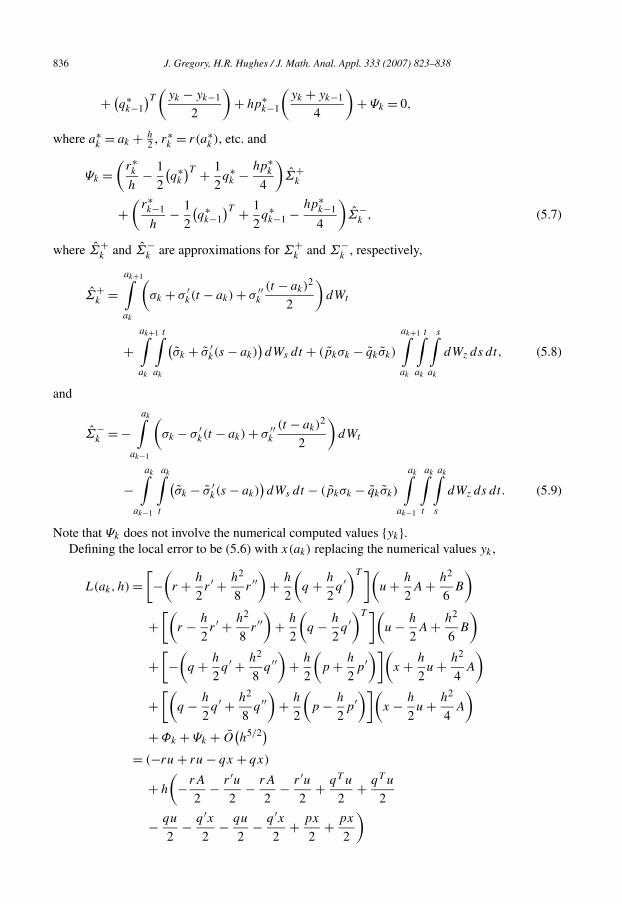
836 J. Gregory, H.R. Hughes / J. Math. Anal. Appl. 333 (2007) 823–838
+ (q∗k−1
)T(
yk − yk−1
2
)+ hp∗
k−1
(yk + yk−1
4
)+ Ψk = 0,
where a∗k = ak + h
2 , r∗k = r(a∗
k ), etc. and
Ψk =(
r∗k
h− 1
2
(q∗k
)T + 1
2q∗k − hp∗
k
4
)Σ+
k
+(
r∗k−1
h− 1
2
(q∗k−1
)T + 1
2q∗k−1 − hp∗
k−1
4
)Σ−
k , (5.7)
where Σ+k and Σ−
k are approximations for Σ+k and Σ−
k , respectively,
Σ+k =
ak+1∫ak
(σk + σ ′
k(t − ak) + σ ′′k
(t − ak)2
2
)dWt
+ak+1∫ak
t∫ak
(σk + σ ′
k(s − ak))dWs dt + (pkσk − qkσk)
ak+1∫ak
t∫ak
s∫ak
dWz ds dt, (5.8)
and
Σ−k = −
ak∫ak−1
(σk − σ ′
k(t − ak) + σ ′′k
(t − ak)2
2
)dWt
−ak∫
ak−1
ak∫t
(σk − σ ′
k(s − ak))dWs dt − (pkσk − qkσk)
ak∫ak−1
ak∫t
ak∫s
dWz ds dt. (5.9)
Note that Ψk does not involve the numerical computed values {yk}.Defining the local error to be (5.6) with x(ak) replacing the numerical values yk ,
L(ak,h) =[−
(r + h
2r ′ + h2
8r ′′
)+ h
2
(q + h
2q ′
)T ](u + h
2A + h2
6B
)
+[(
r − h
2r ′ + h2
8r ′′
)+ h
2
(q − h
2q ′
)T ](u − h
2A + h2
6B
)
+[−
(q + h
2q ′ + h2
8q ′′
)+ h
2
(p + h
2p′
)](x + h
2u + h2
4A
)
+[(
q − h
2q ′ + h2
8q ′′
)+ h
2
(p − h
2p′
)](x − h
2u + h2
4A
)+ Φk + Ψk + O
(h5/2)
= (−ru + ru − qx + qx)
+ h
(− rA
2− r ′u
2− rA
2− r ′u
2+ qT u
2+ qT u
2
− qu − q ′x − qu − q ′x + px + px)
2 2 2 2 2 2

J. Gregory, H.R. Hughes / J. Math. Anal. Appl. 333 (2007) 823–838 837
+ h2(
− rB
6− r ′A
4− r ′′u
8+ rB
6+ r ′A
4+ r ′′u
8
+ qT A
4+ (q ′)T u
4− qT A
4− (q ′)T u
4− qA
4− q ′u
4
− q ′′x8
+ qA
4+ q ′u
4+ q ′′x
8+ pu
4+ p′x
4− pu
4− p′x
4
)
+ Φk + Ψk + O(h5/2)
= Φk + Ψk + O(h5/2), (5.10)
where, except for Φk and Ψk , all evaluations on the right-hand side are made at ak , and where Φ
contains the terms involving Σ− and Σ+,
Φk =(
− 1
hr∗k + 1
2
(q∗k
)T − 1
2q∗k + h
4p∗
k
)Σ+
k
+(
− 1
hr∗k−1 + 1
2
(q∗k−1
)T − 1
2q∗k−1 + h
4p∗
k−1
)Σ−
k . (5.11)
Note that Ψ was defined so that Φk +Ψk = O(h5/2). Since if E and F are the terms that multiplyh and h2, respectively, F = 0 and
E = −rA − r ′u − qu + qT u − q ′x + px
= −r(px + qu) + (p − q ′)x + (qT − r ′ − q
)u = 0.
We have the following:
Theorem 5. If x(t) and u(t) satisfy (5.3), then the local error given in (5.10) satisfies L =O(h5/2).
The arguments in [6] and [8] (deterministic case) and [4] (stochastic case) lead to the desiredpointwise, maximal, global error of O(h) and, under weak additional conditions, O(h3/2).
Defining ek = yk − x(ak) to be the difference between the computed value yk in (5.6) and thesolution of (5.3). For simplicity of exposition, we will assume e0 = e(a) = 0 and eN = e(b) = 0.Let eh = (e1, . . . , eN−1). Subtracting (5.10) from (5.6), we get the three term linear relation inthe components ek ,
(Mheh
)k
.= −r∗k
(ek+1 − ek
h
)− q∗
k
(ek + ek+1
2
)+ r∗
k−1
(ek − ek−1
h
)
+ q∗k−1
(ek + ek−1
2
)+ (
q∗k
)T(
ek+1 − ek
2
)+ hp∗
k
(ek + ek+1
4
)
+ (q∗k−1
)T(
ek − ek−1
2
)+ hp∗
k−1
(ek + ek−1
4
)
= O(h5/2). (5.12)
Let |eh| denote the Euclidean norm of eh and ‖eh‖2 = (E|eh|2)1/2 denote the L2(P ) norm. Themain theorem is as follows.

838 J. Gregory, H.R. Hughes / J. Math. Anal. Appl. 333 (2007) 823–838
Theorem 6. For h > 0 sufficiently small there exists a constant C > 0, independent of h, so that
‖eh‖2 � Ch. (5.13)
The proof of this theorem uses sophisticated results about quadratic forms and symmetricmatrices. See [8] for the details.
Note that Theorem 6 implies that each component of eh is O(h). Furthermore, if each com-ponent of eh is of the same order of magnitude, then each component is O(h3/2). The followingtheorem gives one condition that implies this improved error estimate.
Theorem 7. Suppose that, for h > 0 sufficiently small, the matrix Mh is invertible with eachelement of the inverse bounded by C > 0 independent of h. Then
maxk
∥∥(eh)k∥∥
2 � C′h3/2, (5.14)
for some constant C′ > 0 independent of h.
The proof is similar to the deterministic case which is given in [8].
Acknowledgment
The authors are grateful for the helpful comments of the referee which have led to several improvements in the text.
References
[1] J.M. Bismut, Mécanique Aléatoire, Lecture Notes in Math., vol. 866, Springer-Verlag, Berlin, 1981.[2] M.H.A. Davis, Anticipative LQG control, IMA J. Math. Control Inform. 6 (1989) 259–265.[3] J. Gregory, H.R. Hughes, A new theory and the efficient methods of solution of strong, pathwise, stochastic varia-
tional problems, Methods Appl. Anal. 11 (2004) 303–316.[4] J. Gregory, H.R. Hughes, New efficient numerical procedures for solving stochastic variational problems with a pri-
ori maximum pointwise error estimates, Math. Anal. Appl. (2007), doi:10.1016/j.jmaa.2006.06.021.[5] J. Gregory, C. Lin, Constrained Optimization in the Calculus of Variations and Optimal Control Theory, Van Nos-
trand Reinhold, New York, 1992.[6] J. Gregory, C. Lin, Discrete variable methods for the m-dependent variable, nonlinear extremal problem in the
calculus of variations, II, SIAM J. Numer. Anal. 30 (1993) 871–883.[7] J. Gregory, C. Lin, An unconstrained calculus of variations formulation for generalized optimal control problems
and for the constrained problem of Bolza, J. Math. Anal. Appl. 187 (1994) 826–841.[8] J. Gregory, R.S. Wang, Discrete variable methods for the m-dependent variable, nonlinear extremal problem in the
calculus of variations, SIAM J. Numer. Anal. 27 (2) (April 1990) 470–487.[9] L.M. Hocking, Optimal Control: An Introduction to the Theory with Applications, in: J.N. Buxton, R.F. Church-
house, A.B. Taylor (Eds.), in: Oxford Applied Mathematics and Computing Science Series, Clarendon Press,Oxford, 1991.
[10] D.E. Kirk, Optimal Control Theory: An Introduction, in: R.W. Newcomb (Ed.), in: Electrical Engineering Series,Prentice Hall, Inc., Englewood Cliffs, NJ, 1970.
[11] G. Leitmann, The Calculus of Variations and Optimal Control, in: A. Miele (Ed.), Mathematical Concepts andMethods in Science and Engineering Series, Plenum Press, New York, 1981.
[12] D. Nualart, The Malliavin Calculus and Related Topics, Springer-Verlag, New York, 1995.[13] B. Øksendal, Stochastic Differential Equations: An Introduction with Applications, fourth ed., Springer, Berlin,
1995.[14] H. Sagan, Introduction to the Calculus of Variations, Dover Publications, New York, 1969.