The efficiency of theatres in Finland - Myy...

1

The efficiency of theatres in Finland Seppo Suominen, Haaga-Helia University of Applied Sciences, Helsinki, Finland

Contents The efficiency of theatres in Finland ................................................................................................................. 1

The efficiency of theatres in Finland ................................................................................................................. 2

1 Introduction ........................................................................................................................................... 2

2 Different approaches for efficiency ....................................................................................................... 5

3 The data and model specification ....................................................................................................... 13

4 Results ................................................................................................................................................. 16

Evaluation .................................................................................................................................................... 23

References ................................................................................................................................................... 25

Appendix .......................................................................................................................................................... 28

2

The efficiency of theatres in Finland

1 Introduction

The theatre and orchestra law (705/92) that has come into force in 1993 brought considerable changes to theatre

financing in Finland. The state subsidy to the dramatic art had been discretionary until 1993 and mainly financed

by profit funds of the pools and money lotteries. Since the beginning of 1993 the Ministry of Education has

made theatre-specific decisions on state subsidies. The basic principle in the state subsidy system (VOS)1 is that a

theatre receives subsidies on the grounds of unit cost based on full time equivalent (FTE) person years. The

reason for this change in 1993 was that theatres could make long-range artistic work with a sounder financial

situation. In 1993 the number of theatres in this state subsidy system was 53 in Finland. Almost all theatres

established during the 1960’s and 1970’s were included in this system. However, many “second generation”

theatre groups established in the 1990’s were left outside (Kanerva and Ruusuvirta 2006, 9). In 2007 the number

of theatres within this system was 58 so that 46 were speech theatres (including the National Theatre) and 11

dance theatres. In addition to these, The National Opera is along in the system. All together the state subsidies

(“funding bill”) to the theatres and orchestras in 2007 were about 47M€ and to the National Opera about 31M€.

In addition to this some minor theatre groups received discretionary about 1,5M€ state subsidies. Also the

municipalities support the above mentioned institutions and groups with about 63M€. In practice this means that

the income share of state and municipal subsidies was 25 % and 43 % for theatres excluding the National

Theatre and the National Opera. The share of other incomes (sales of the programme, interest revenue) was

about 5% and the rest, i.e. 28% comes from ticket revenues. The state subsidy system can be justified by the

Baumol’s cost disease (Baumol and Bowen 1966). Labour productivity progress in cultural sectors, especially in

the theatre is low since live performing arts are labour intensive. While labour costs of producing a performance

increase over time in line with the other sector of the economy, labour productivity will remain unchanged.

Increases in labour productivity over time may occur since there is (1) increased capital per worker, (2) improved

technology, (3) increased labour skill, (4) better management, and (5) economies of scale (Heilbrun 2003). Capital

1VOS = (in Finnish) valtionosuuslainsäädäännön piiriin kuuluva ~ theatres subsidised by law

3

enhancement in the theatre can improve the management (ticket sales through internet) and technical aspects of

the performance by stage lighting and air conditioning but since the performer’s labour is the output – the pianist

playing, the actor acting, the singer singing – there is no way to increase output per hour2. It takes at least seven

male actors to perform the famous play by Aleksis Kivi “Seitsemän veljestä” (Seven brothers) today as it did in

1898. As a result, performing arts institutions will have financial difficulties since costs will increase relative to

revenues (Zieba and Newman 2007). Still technology can increase the size of the audience via online

performance transmissions to movie theatres around the world from the Metropolitan Opera, New York. Opera

performances are suitable for online transmissions since it is usual that the performance is presented in the

original language (i.e. Italian, German, French, etc.) and the audience has got used to it all over the world.

The change in the FTE person years as criteria for state and the true (verified) person years have not been

equivalent over the years since 1993. The true change is higher than the criteria. Also the change in the unit cost

as criteria for state and the verified unit cost has been lower3, however, during the last two decades the change

(growth) in state subsidies and ticket revenues has been substantially higher than the change in municipal

subsidies (Kangas and Kivistö 2011, 17). The above mentioned law came into force 1993, and the financing

structure of theatres changed considerably. The state aid increased by about 50 per cent and correspondingly the

municipal share dropped. During the years from 1993 to 2007 considerable changes did not take place but the

unit cost standard was substantially changed a few years ago, and the state aid increased by more than 15 per cent

annually during the years 2008 to 2010 (Tinfo, statistics). The raising of the unit cost returned its real value to the

1993 level (Kangas and Kivistö 2011, 11). The state support is directed to the administrator of the culture

institution, municipality or federation of municipalities, to a private community or foundation. As a rule the state

subsidy is 37 per cent of the price of the person year with certain exceptions4. Since the share of public subsidies

is so big, it is important that these cultural institutions and groups should pursue efficiency and respect high

quality and cultural diversity. Most of plays in theatres are spoken plays but from the point of view of incomes

2 This may explain why the share of permanent artistic staff is gradually lowering and theatres seem to use more temporary staff (freelancers). 3 Report of a committee on the system of statutory state aid granted to theatres, 2003, 23, 26 4 During the years 1993 and 1995 the state aid was determined by the financial classification of the location municipality of the theatre and it varied between 25 – 40 per cent. The state aid to Tampereen työväen teatteri (the only professional workers theatre in Finland) and to Svenska Teatern i Helsingfors (the biggest Swedish speaking theatre) is 60 per cent (Report of a committee on the system of statutory state aid granted to theatres, 2003, 18)

4

the musical plays are important since they appeal to the public.5 On the other hand, musical plays might be more

expensive since the artistic staffs consist of not only actors but also musicians.

According to the ownership, the theatres can be classified into full municipal theatres (11) and private theatres.

Some of the private theatres, however, serve as a part of the municipality conglomerate in which case the privacy

brings about some financial independence in comparison with other municipal bodies like primary school or

local health care centre. The administrative models of theatres are mostly an association, a foundation or a

limited company. The National theatre which is mainly financed by the state is a limited company with a

foundation as formal owner. The Finnish National Opera is governed by the Foundation of the Finnish National

Opera and 70 per cent of the funding comes from the state. The theatre management see the advantage of the

privacy as less bureaucracy and increase in the freedom of theatres (Kanerva and Ruusuvirta 2006, 11).

The measurement of the achievement of the cultural institutions is complicated by the presence of goals of

different nature. The principal objectives and obligations set to the VOS-theatres are related to regular

presentation activity, to spectator number and to the number of premieres or performances (Kanerva and

Ruusuvirta 2006, 88). It is troubled to measure the achievement of the theatre due to the multiple goals. On one

hand, it is important that there are many visitors, since it has been shown that scale economies exist (Taalas

1997) and average costs decline, however, on the other hand, it is also important that there are many

performances and many different plays since the cultural diversity increases. This in turn can lead to allocative

inefficiency. Taalas (1997) proposes that on average in Finland the actual total costs exceeded the minimum cost

by some 5 per cent in the 1980’s and 1990’s. The non-optimal usage of inputs may originate from the managers’

desire for big audiences, big budgets and high quality of production. Performances offer viewers cultural

experience but also entertainment. The theatregoers prefer large productions in terms of cast size (Werck and

Heyndels 2007) and less esoteric performances (Jenkins and Austen-Smith 1987). The reputation of the author,

producer and cast has a positive impact on the spectator number (Abbé-Decarroux 1994). Cultural diversity in

terms of the number of productions in a theatre is associated with public subsidies. Higher public funding is

5 During the theatrical seasons 2007/2008 – 2009/2010 the musical plays’ share of performances was on average 14-15 % while the share of sold tickets was 25-29 %. Plays for children and youth and puppet plays had a lower sold ticket share than their share of performances.

5

positively related to the number of productions a theatre mounts and negatively related to the conventionality of

theatre programs (Austen-Smith 1980, DiMaggio and Stenberg 1985, O’Hagan and Neligan 2005, Werck, Stultjes

and Heyndels 2008). On the other hand, a bigger budget which is partially financed by public subsidies leads to

higher cast and therefore to bigger audience (Werck, Stultjes and Heyndels 2008). Other indicators set to the

VOS-theatres are a euro-denominated sales objective and a versatile, interesting and high-quality programme as

such (Kanerva and Ruusuvirta 2006, 89). In the biggest towns the theatres have segmented according to

objectives and for example there is own programme for children, e.g. puppet theatre. In bilingual municipalities

(Finnish and Swedish) the presentations are expected on both domestic languages. For private theatres the

objectives are specified usually between the municipality and the theatre every year in connection with

acceptance of the municipal budget. The objectives can be based and they can be included to the service

agreement in which the common goals are set. The subscriber-producer (public-private partnership) or the

service agreement defines carefully the charges and indicators. The representatives named by the municipality

can be members in the board of the private theatres (Kanerva and Ruusuvirta 2006, 89).

Since the measurement of achievements in subsidised is versatile, the research question in this essay is to study is

the efficiency ordering similar when different measures or methods are used and which inputs are relevant in

arranging the sequence of theatres. All of these questions are important for the socially optimal subsidising

system.

The rest of the paper is organized as follows: section 2 and 3 present different approaches for efficiency and the

data and model specification. Section 4 presents the results and the implications. Section 5 provides the

conclusions.

2 Different approaches for efficiency

6

Since the objectives and therefore achievement measurement is versatile, different measures have been used in

the theatre efficiency literature. Two approaches have been used. A non-parametric technique data envelopment

analysis (DEA) is useful since there is no need to explicitly specify a mathematical form for the production

function. The DEA approach is based on the pioneering work of Farrell (1957), Charnes, Cooper and Rhodes

(1978) and Färe, Grosskopf and Lovell (1985). The other approach is to use a statistical method. This method

assumes that efficiency follows a certain statistical distribution and there is some functional form for the

efficiency frontier (Kirjavainen 2009, 19). Since the statistical approach assumes that there is a relationship

between inputs and output, the effect of each input can be evaluated with statistical significance testing.

A non-parametric DEA is capable of handling multiple inputs and outputs and the sources of inefficiency can be

analysed and quantified for each evaluated theatre (Marco-Serrano 2006, 171). In DEA, the efficiency frontier is

estimated as a linear combination of inputs and outputs (Coelli et. al 2005, 162). For each theatre the efficiency is

valued relative to the frontier. The deviation from the frontier is defined as inefficiency. Technical efficiency is

defined as the ratio of observed output(s) to maximum potential output(s) achievable from the given inputs

(output oriented efficiency) or as the ratio of the minimum potential input(s) to observed input(s) required to

produce the output(s) (input oriented efficiency). Cost efficiency takes the input prices (wage, unit cost of capital

or “price of one seat”, etc.) into account. Allocative efficiency examines revenues and requires that theatres are

technically efficient and produce their outputs by maximising their revenues. Cost efficiency and allocative

efficiency are two approaches to economic efficiency. Cost efficiency is input oriented and allocative efficiency is

output oriented. Allocative inefficiency is caused by the wrong mixture of inputs in use (Farrell 1957, 254). The

allocative inefficiency measure is sensitive with respect to new observations and measurement error, therefore

the measure is unstable (Farrell 1957, 261). The overall efficiency is a combination of technical and allocative

(cost) efficiencies. The technical efficiency can be decomposed into two elements: pure technical efficiency and

scale efficiency assuming variable returns to scale. The scale efficiency indicates if the management is operating

in the right scale. In the case of constant returns to scale, the decomposing is irrelevant.

7

Mathematically the measurement of efficiency (eff) in DEA is defined as ratio of weighted sum of outputs (α’yi)

to a weighted sum of inputs (β’xi) for firm i (eff = α’yi/β’xi) where yi is the vector of M outputs and xi is the

vector of K inputs. The optimal weights are defined by the programming problem

(1) Maximize wrt α,β: α’yi/β’xi

Subject to α’ys/β’xs ≤ 1, s = 1, ... , N

αm ≥ 0, m = 1, ... , M

βk ≥ 0, k = 1, ... , K

The optimization program finds the optimal weights (α,β) to maximize the efficiency of firm s. Since the

objective function is homogenous of degree zero, any multiple of the weights produces the same solution (Coelli

et al 2005, 163). The envelopment form is an equivalent form of the problem:

(2) Minimize wrt θi, λ: θi

Subject to Σsλsys – yi ≥ 0

θixi – Σλsxs ≥ 0

λs ≥ 0

The value of θi is the input oriented technical efficiency score for the firm i. Due to mathematical nature of the

problem solution, the efficiency score θi will be 1.0 for some firm(s) in the sample and for the others it will be

less than one. However, the above implicitly assumes constant returns to scale. This is relaxed by adding a

restriction Σsλs = 1 to variable returns to scale which is more plausible in the case of theatre performances (Ek

1991, Kokkinen 1997). Let θiC stand for the technical efficiency score assumed constant returns and θiV be the

variable returns to scale measure. Then the scale efficiency is the ratio of these measures: θiC/θiV.

The output oriented view of the optimization is to consider inputs as given. The linear program for this is

assuming constant returns to scale:

(3) Maximize wrt φi, λ: φi

Subject to Σsλsys – φiyi ≥ 0

xi – Σλsxs ≥ 0

λs ≥ 0

8

The variable returns to scale model is obtained by adding the constraint: Σsλs = 1. The technical efficiency

measure is 0 < 1/φi ≤ 1. One firm or some firms will be technically efficient and the others are inefficient

relative to the frontier firms (Coelli et al 2005, 180).

With input price w information a corresponding optimization (cost minimization) problem can be constructed.

(4) Minimize wrt χi,λ: wi’χi

Subject to Σsλsys – yi ≥ 0

χi – Σλsxs ≥ 0

λs ≥ 0

The linear optimization solution for χi is the cost minimizing vector of inputs given the output yi and the input

prices wi. The cost efficiency for firm i is the ratio 0 < wiχi/wi’xi < 1. Allocative efficiency could be measured by

ratio of cost efficiency and input oriented technical efficiency: [wiχi/wi’xi]/θi < 1.

With Finnish theatre data covering the years 1987 – 1995 Kokkinen (1997) studied the efficiency of theatres with

four outputs and one input using DEA. The list of outputs was: the number of premieres, the number of

performances, sold tickets and ticket revenue. The only input was total costs excluding real property costs. The

results indicate that full municipal theatres have the lowest efficiency scores, both in terms of the pure technical

efficiency and the scale efficiency. A big majority of the theatres have had diminishing returns to scale

throughout the sample period. Due to data limitations allocative or cost efficiencies could not be estimated. It is

noteworthy that on the average efficiency is rather low and there are substantial differences in efficiency scores.

The high average inefficiency level is also found out by Marco-Serrano (2006) with Spanish regional theatres data

for 1995 – 1999 using DEA framework. The output variables were the number of performances and/or the

number of attendances and the input variables were venue capacity, the number of different performed plays,

total paid to the performing company and the amount subsidised by the Spanish municipality network. The

problem with DEA is that there is no statistical significance testing for choosing the relevant input variables. If

9

the efficiency is a managerial problem, the managers of the theatres should be able to control these inputs;

however, the managers cannot control the environmental related variables, e.g. educational level of the region.

Several surveys have shown that women and high educated go more often (Suomen teatteriliitto 2001, 2004,

Suomen Teatterit ry 2007). Otherwise the literature on the efficiency of theatres using DAE is extremely scarce.

Besides those mentioned above there are only few studies with Swedish and German data (Ek 1991a, 1991b,

1994, Tobias 2003).

It is important to use the averages of a few years to diminish the stochastic variation of observations since DEA

is very sensitive to outliers. The efficiency frontier might be occasional and thus uncertain when there are outliers

in the data6. Tobias (2003) argues that there is a substantial savings potential when public theatres would be

privatized. However, the main problem with DEA is that the statistical significance testing of each input variable

is limited. One approach to solve this problem is to use bootstrapping to get confidence limits for the estimated

efficiency scores (Simar and Wilson 1998). The DEA bootstrapping methods are, however, designed to deal

with sampling variability (Coelli et al 2005, 202) not with input variable significance testing. Despite the

shortcomings DEA is useful since it distinguishes efficient firms from inefficient. A suitable approach is to

include only those inputs that are controllable by the management to DEA in the first stage. In the second stage

the efficiency scores obtained from the first stage are statistically explained with environmental variables that

might cause the inefficiency (Pitt and Lee 1981 or recently Kirjavainen 2009).

The statistical approach has two main routes both assuming some functional form for the production

relationship. The common used functional forms are linear, the Cobb-Douglas, and the translog due to their

convenience. The technological change or substitutability of inputs or other relevant indicators are easily

6 Achievement in terms of the number of performances or sold tickets in each VOS-theatre including the National theatre and the National Opera throughout the recent years has been stable as the correlation statistics (below) reveals:

n = 58 perf2007 perf2008 perf2009 perf2010 soldtic07 soldtic08 soldtic09 soldtic10

perf2007 1 soldtic07 1

perf2008 0.975 1 soldtic08 0.977 1

perf2009 0.970 0.976 1 soldtic09 0.947 0.983 1

perf2010 0.955 0.949 0.951 1 soldtic10 0.941 0.971 0.983 1

10

estimated. For example, using a generalised cost function7 Taalas (1997) shows with Finnish theatre data for

years 1985-1993 that observed costs exceed the minimum costs by about 5 per cent. Scale economies exist and it

is more cost effective to run a play longer than change the repertoire. Old productions are cheaper since certain

fixed costs like scenery and costumes related costs can be avoided. Also size economies exist and diminishing

average costs in the supply of seat capacity has been found in several studies (Baumol and Bowen (1996) for US

symphony orchestras, Globerman and Book (1974, 1977) for Canadian theatres and orchestras, Gray (1992) for

Norwegian theatres, Hjort-Andersen (1992) for Danish theatres). Thus a bigger capacity and a longer run for a

play is more cost efficient. Conventional least squares estimator (OLS) and maximum likelihood estimators are

identical in the case of linear regression models, e.g. taking logarithms of the above mentioned Cobb-Douglas or

translog forms.

(5) Cobb-Douglas: 𝑙𝑛𝑦𝑖 = 𝐴0 + ∑ 𝛽𝑛𝑙𝑛𝑥𝑛𝑁𝑛=1 + 𝑢𝑖

(6) Translog 𝑙𝑛𝑦𝑖 = 𝐴0 + ∑ 𝛽𝑛𝑙𝑛𝑥𝑛𝑁𝑛=1 + ½ ∑ ∑ 𝛽𝑛𝑚𝑙𝑛𝑥𝑛

𝑀𝑚=1

𝑁𝑛=1 𝑙𝑛𝑥𝑚 + 𝑢𝑖

The efficiency can be assessed by measuring the distance of a theatre from the achievement function. The OLS

residual (ui) provides a measure of each theatre’s achievement. The achievement function estimated by OLS is an

average of the observed points of all theatres. To get the frontier above the observations, a corrected OLS can

be applied (Johnes 2006). In this case, the equation (e.g. the Cobb-Douglas form or the translog form) is

estimated using OLS, and then the intercept A0 is shifted up until the residuals are non-positive and at least one

is 0. The ranking of the theatre efficiency, however, remains identical to that obtained from OLS. Several studies

have empirically evaluated the cost structure of theatres (Globerman and Book 1972, 1974, 1977 and Gray 1992,

Hjort-Andersen 1992) but the efficiency frontier analysis using least squares or similar approach is sparse. It is

easier to estimate the relationship between costs and output given that the output is unambiguous which is not

always so clear due to different objectives set to theatres by the subsidising authorities. The problem with these

deterministic frontier models is that all deviations from the frontier are assumed to be the result of inefficiency.

The measurement errors and other sources of statistical noise are not taken into account (Coelli et al 2005, 242).

7 𝑙𝑛𝑐𝑎 = 𝛼0 + 𝛼𝑦𝑙𝑛𝑦 + 𝛾𝑦𝑦(𝑙𝑛𝑦)2 + ∑ 𝛼𝑖𝑙𝑛(𝑣𝑖𝑖 𝑝𝑖) + ∑ ∑ 𝛾𝑖𝑗𝑙𝑛(𝑗𝑖 𝑣𝑖𝑝𝑖) 𝑙𝑛(𝑣𝑗𝑝𝑗) + ∑ 𝛾𝑦𝑖𝑖 𝑙𝑛𝑦𝑙𝑛(𝑣𝑖𝑝𝑖) +

ln[∑ 𝑣𝑖−1

𝑖 (𝛼𝑖 + 𝛾𝑦𝑖𝑙𝑛𝑦 + ∑ 𝛾𝑖𝑗𝑗 ln(𝑣𝑖𝑝𝑗))] , 𝑖 = 1,2 where vi are the proportions of which the shadow price of the ith

input differs from the market price pi

11

Aigner, Lovell and Schmidt (1977) and also Meeusen and van den Broeck (1977) autonomously presented the

stochastic frontier model which in the case of the Cobb-Douglas form is:

(7) 𝑙𝑛𝑦𝑖 = 𝐴0 + ∑ 𝛽𝑛𝑙𝑛𝑥𝑛𝑁𝑛=1 + 𝑣𝑖 − 𝑢𝑖

In which vi is a symmetric random error to account for statistical noise and ui is a measure of inefficiency. 𝐴0 +

∑ 𝛽𝑛𝑙𝑛𝑥𝑛𝑁𝑛=1 is the deterministic part of the frontier and vi ~ N(0,σv

2) is the stochastic part. The two parts

together is the stochastic frontier. Aigner, Lovell and Schmidt (1977) obtained the estimates assuming ui ~

N+(0,σu2). The latter assumption (the half-normal) is the basic assumption in the stochastic frontier analysis.

Aigner, Lovell and Schmidt (1977) defined σ2 = σv2 + σu

2 and λ2 = σu2/ σv

2 ≥ 0. If λ = 0, there are no technical

inefficiency effects and deviations from the frontier are caused by noise (Coelli et. at 2005, 246).

A large range of different assumption on the distribution of the inefficiency term, such as half normal or

exponential with mean λ (Aigner, Lovell, Schmidt 1977), truncated normal with mean μ (Stevenson 1980),

gamma with mean λ and degrees of freedom m (Greene 1990). The ranking of inefficiencies is similar in most

cases regardless of the distributional assumption (Kumbhakar and Lovell 2000, 90). However, both the half

normal and exponential distributions have a high density near zero, implying that the technical efficiency of the

firms is in the neighbourhood of one (Coelli et. at 2005, 252). The truncated normal and gamma distributions are

more flexible in the sense of efficiency distributions.

If the efficiency frontier is occasional due to time specific reasons, a cross-section analysis might be biased. To

solve the problem, a panel data approach can be used. The panel data incorporates both the time-series and

cross-section dimensions. It is possible that the stage is under renovation or the technical staff and clothes

guards are on strike. It has been argued that inefficiency values might be overestimated due to unobserved firm-

specific heterogeneity in achievement measurement (Farsi, Filippini and Greene 2005, Greene 2005).

Unobserved firm-specific heterogeneity can be taken into account with fixed or random effects in a panel data

12

approach. Panel data version of the Aigner, Lovell and Schmidt (1977) model in Cobb-Douglas form can be

written:

(8) 𝑙𝑛𝑦𝑖𝑡 = 𝐴0 + ∑ 𝛽𝑛𝑙𝑛𝑥𝑛𝑡𝑁𝑛=1 + 𝑣𝑖𝑡 − 𝑢𝑖𝑡

which is otherwise identical to (7) expect that a subscript “t” has been added to represent time (Coelli et al 2005,

275). The inefficiency parameter uit is either a fixed parameter over time or a random variable. The

corresponding models are known as fixed effects model (Schmidt and Sickles 1984) and a random effects model

(Pitt and Lee 1981). The fixed effects model can be estimated using a dummy variable for each firm and

dropping out the constant term A0 to avoid perfect collinearity (Greene 2005). The fixed effects model, however,

results in much lower efficiency levels than the random effects model (Kim and Schmidt 2000). Still the fixed

effects model is useful since the estimated coefficients are not affected by any correlation between the time

varying explanatory variables and the firm-specific effects (Greene 2005). The inefficiency of the firms can be

measured only relative to the best firm(s) in the sample and the inefficiency estimates are sensitive to sample

selection and outliers (Farsi and Filippini 2004).

The random effects model proposed by Pitt and Lee (1981) assumed a half normal distribution8 for the

inefficiency parameter uit ~ N+(0, σu2) in which the efficiency scores might cluster around one. Battese and Coelli

(1988) proposed using a more general truncated normal distribution. uit ~ N+(μ, σu2). However, any time-

invariant firm-specific unobserved heterogeneity is included in the firm-specific component and uncorrelated

with the variables included in the model. The conventional fixed and random effects models tend to

overestimate the inefficiency if any time-invariant firm-specific unobserved heterogeneity exists (Greene 2005).

The true random effects model proposed by Greene (2005) accounts for the shortcomings of the conventional

fixed effects and random effects panel data models by adding a firm-specific random term ai

(9) 𝑙𝑛𝑦𝑖𝑡 = 𝐴0 + 𝑎𝑖 + ∑ 𝛽𝑛𝑙𝑛𝑥𝑛𝑡𝑁𝑛=1 + 𝑣𝑖𝑡 − 𝑢𝑖𝑡

8 The probability density function of a half-normal distribution is truncated version of a normal random variable having zero mean and variance σu

2. Commonly the half-normal distribution is replaced with truncated normal or with gamma distribution with mean λ and m degrees of freedom: uit ~ G(λ,m). The exponential distribution with mean λ: uit ~ G(λ,0) is a special case of gamma distribution. Sometimes the assumption of half-normal distribution is not suitable since it implies that most inefficiency effects are in the neighbourhood of zero (Coelli et. al, 2005, 252).

13

The firm-specific unobserved heterogeneity ai is time-invariant and uit represents time-varying firm-specific

inefficiency. Any persistent inefficiency is not included in the inefficiency term since all time-invariant effects are

treated as unobserved heterogeneity. The true random effects tends to underestimate the inefficiency since at

least part of the time-invariant factors considered as external heterogeneity are related to inefficiency (Farsi,

Filippini and Greene 2006).

3 The data and model specification

The data set is a balanced panel of Finnish VOS-theatres (theatres subsidised by law) covering the seasons

2006/07 – 2010/11. The primary data is taken from the statistics collected and published by Theatre Info

Finland (Tinfo). Some auxiliary data is from official statistics Finland. The output measure in the DEA method

can include several indicators from volume to versatility. The performances or the number of tickets sold during

the season or the number of spectators are volume measures, while the versatility has been measured by

Herfindahl-Hirschman index9 of diversity. In this index the shares of different categories of plays are squared. If

a theatre has only spoken plays but no musicals or plays for children, the diversity is low. However, if the theatre

has a wide range of categories from spoken plays to puppet shows, the diversity is high. It is possible that there is

a trade-off between versatility and volume. Due to difficulty of classification the versatility is measured simply by

the number of different plays during the season. Non-profit performing arts institutions could be regarded as

output maximizes with quality having an important role (Thorsby 2010). Most VOS-theatres in Finland are

repertory theatres. Each production is performed several times during the season and many productions are run

simultaneously. There is one dance theatre in Finland – Zodiak, “Center for New Dance” – in the state

subsidiary system in which the number of new productions has bigger role than re-runs. The repertoire of the

speech theatres varies seasonally from 2 to 39, the mean is 11. The bigger theatres have a larger repertoire.

In the case of statistical approach it is reasonable to model the production technology as an input distance

function in which the efficiency is the ratio of output to a vector of inputs. The distance function approach is

reasonable if producers use multiple inputs to produce multiple outputs, like the spectator number and the

9 HH index has been used by Heilbrun, JCult2001

14

number of different performances. These outputs could be substitutes if a popular play attracting a wide

spectator number is replaced with a new (but not popular) play. Hence the number of different plays might

reduce the overall spectator number, however the opposite is also possible if the popular play is reaching its

maximum attendance and it is not continued any longer and replaced with a new play. This optimal duration of

the run is a talent that some theatre managers have and some do not have. Since the panel data has only five

years, it is reasonable to assume that the inefficiency levels which are theatre specific will not vary over time.

Therefore the technological progress is not estimated.

The cost function approach might not be sensible since it presumes cost minimisation behaviour which is

probably not valid due to heavy subsidies from the state and municipalities. These inputs in the distance

approach are related to artists, scenery and décor, technical staff. The staffs are employed on a full-time or part-

time basis and the contracts are permanent or temporary. Following Last and Wetzel (2010) and ignoring time

the stochastic frontier function for K (k = 1… K) inputs and M (m = 1, …, M) outputs can be written as

(10)

𝑙𝑛𝐷𝑖𝑡 = 𝛼 + ∑ 𝛽𝑚𝑙𝑛𝑞𝑚𝑖𝑡

𝑀

𝑚=1

+ 1

2∑ ∑ 𝛽𝑚𝑛𝑙𝑛𝑞𝑚𝑖𝑡

𝑁

𝑛=1

𝑀

𝑚=1

𝑙𝑛𝑞𝑛𝑖𝑡 + ∑ 𝛽𝑘𝑙𝑛𝑥𝑘𝑖𝑡

𝐾

𝑘=1

+ 1

2∑ ∑ 𝛽𝑘𝑙𝑙𝑛𝑥𝑘𝑖𝑡

𝐿

𝑙=1

𝐾

𝑘=1

𝑙𝑛𝑥𝑙𝑖𝑡

+ ∑ ∑ 𝛾𝑘𝑚𝑙𝑛𝑥𝑘𝑖𝑡

𝑀

𝑚=1

𝐾

𝑘=1

𝑙𝑛𝑞𝑚𝑖𝑡 + ∑ 𝜇𝑠𝑧𝑠𝑖𝑡

𝑆

𝑠=1

where the subscripts i and t indicate the theatre and year. Dit is the input distance term, xkit and qmit denote the

input and output quantity and zsit indicate observable theatre characteristics that have an impact on the

production technology, and 𝛼, 𝛽, 𝛾 and 𝜇 are unknown parameters to be estimated. In the input distance

function some restrictions must hold: for symmetry 𝛽𝑚𝑛 = 𝛽𝑚𝑛 and 𝛽𝑘𝑙 = 𝛽𝑙𝑘 and for linear homogeneity in

inputs ∑ 𝛽𝑘 = 1, ∑ 𝛽𝑘𝑙 = 0, 𝐾𝑙=1 ∑ 𝛾𝑘𝑚 = 0. 𝐾

𝑘=1𝐾𝑘=1 Setting the homogeneity structures by normalising the

distance term Dit and the inputs in (10) and replacing the log of the distance term 𝑙𝑛𝐷𝑖𝑡 with an error term −𝜀𝑖𝑡

the translog input distance can be estimated. The function can be written as

15

(11)

−𝑙𝑛𝑥𝐾𝑖𝑡 = 𝛼 + ∑ 𝛽𝑚𝑙𝑛𝑞𝑚𝑖𝑡

𝑀

𝑚=1

+ 1

2∑ ∑ 𝛽𝑚𝑛𝑙𝑛𝑞𝑚𝑖𝑡

𝑁

𝑛=1

𝑀

𝑚=1

𝑙𝑛𝑞𝑛𝑖𝑡 + ∑ 𝛽𝑘𝑙𝑛𝑥𝑘𝑖𝑡∗

𝐾−1

𝑘=1

+ 1

2∑ ∑ 𝛽𝑘𝑙

𝐿−1

𝑙=1

𝐾−1

𝑘=1

𝑙𝑛𝑥𝑘𝑖𝑡∗ 𝑙𝑛𝑥𝑙𝑖𝑡

∗ + ∑ ∑ 𝛾𝑘𝑚𝑙𝑛𝑥𝑘𝑖𝑡∗

𝑀

𝑚=1

𝐾−1

𝑘=1

𝑙𝑛𝑞𝑚𝑖𝑡 + ∑ 𝜇𝑠𝑧𝑠𝑖𝑡

𝑆

𝑠=1

+ 𝜀𝑖𝑡

where 𝑥𝐾𝑖𝑡∗ = (

𝑥𝑘𝑖𝑡

𝑥𝐾𝑖𝑡). The input distance function must be non-decreasing in inputs and non-increasing in

outputs indicating that

(12) 𝜕𝑙𝑛𝐷

𝜕𝑙𝑛𝑥𝑘= 𝛽𝑘 + ∑ 𝛽𝑘𝑙

𝐿𝑙=1 𝑙𝑛𝑥𝑙 + ∑ 𝛾𝑘𝑚

𝑀𝑚=1 𝑙𝑛𝑞𝑚 ≥ 0 and

(13) 𝜕𝑙𝑛𝐷

𝜕𝑙𝑛𝑞𝑚= 𝛽𝑚 + ∑ 𝛽𝑚𝑛

𝑁𝑛=1 𝑙𝑛𝑞𝑚 + ∑ 𝛾𝑘𝑚

𝐾𝑘=1 𝑙𝑛𝑥𝑘 ≤ 0

The ability of a theatre management to convert inputs into outputs is influenced by environmental and

exogenous variables in which the production takes place. Pitt and Lee (1981) use a two-stage approach. The first

estimation uses a conventional frontier model excluding the environmental variables. The inefficiency scores are

calculated using a standard formula (below):

(14) 𝑇𝐸𝑖𝑡 = exp (−𝑢𝑖𝑡)

The second stage involves regressing these calculated inefficiency scores on the environmental variables. The

other approach is to include these environmental variables in the first stage (Coelli, et al. 282, 2005). The theatre

characteristics here refer to both controllable and environment variables that must be taken by the management

of the theatre. The management of the theatre is able to control the ticket price but they have no control over

e.g. the population of the area, the educational level or the incomes of the population and the competition

situation in the area. Zieba (2011) shows that the exogenous variables have an important impact on the technical

efficiency scores.

The output is complicated as described in the introduction. The artistic value of the production is not observed

and cannot be measured directly. We observe only quantities such as the number of performances, the number

16

of tickets sold or the number of seats available for the entire season (seats in the stages times the number of

performances). Since the attendance is an experience good, the output is often measured by the number of

tickets sold assuming that the quality of the performance is revealed through the word-of-mouth. Since a single

play is performed several times during the season, the early visitors advise their friends about the quality of the

play. Positive signals from the early visitors increase the attendance later. The premiere attendance is not

measuring the quality of the performance since the word-of-mouth is lacking. However, since different output

measures are available, these are used in different estimations.

4 Results

The first table presents the stochastic frontier analysis (SFA) results when the output (y1) is tickets sold using a

fixed effects or random effects or true random effects model without restrictions. The dependent variable, -lnxKit

is the logarithm of the number of the actors with negative sign. The half-normal distribution assumption for the

uit is used in the estimations. Following Zieba (2011) one exogenous variable is included in the estimation and

hence the Pitt-Lee two stage approach is not used. Also the ticket price is included. The management of the

theatre house predetermines the ticket price of each act as well as it determines the plays in the repertoire. The

Wald test for the restrictions is included in the table 1.

Variable (all in logarithmic) / parameter

Fixed effects

Random effects True random effects; 50 Halton draws

Fixed effects Random effects (with two restrictions)

y1 = Tickets sold / βy1

-2.11 (0.194)***

-1.65 (0.446)***

-1.62 (0.242)***

-1.99 (0.197)***

-1.57 (0.475)***

y12 / βy1y1 0.0855 (0.0135)***

0.0644 (0.0205)**

0.0639 (0.0118)***

0.101 (0.0141)***

0.0801 (0.0220)***

x2 = Other staff/actors / β2

0.321 (0.152)*

0.242 (0.188)

0.248 (0.115)*

0.391 (0.154)*

0.311

x22 / β22 -0.0366 (0.00222)***

-0.0364 (0.00440)***

-0.0329 (0.00198)***

-0.0406 (0.00269)***

-0.0400

x3 = seat capacity/actors / β3

-0.135 (0.270)

-0.0403 (0.609)

-0.0683 (0.300)

0.717 (0.289)*

0.689 (0.258)***

x32 / β33 -0.0557 (0.0320)(*)

-0.0465 (0.0419)

-0.0556 (0.0203)**

0.0222 (0.0357)

0.0328 (0.0218)

x2x3 / β23 -0.0484 (0.0133)***

-0.0436 (0.0241)(*)

-0.0129 (0.0176)

0.00695 (0.0141)

0.00722 (0.0238)

y1x2 / γ12 -0.0341 (0.0145)*

-0.0275 (0.0196)

-0.0331 (0.0108)**

-0.0560 (0.0150)***

-0.0478 (0.0221)*

y1x3 / γ13 0.0931 (0.0302)**

0.0761 (0.0510)

0.0727 (0.0271)**

-0.0510 (0.0227)

-0.0550 (0.0217)*

average ticket price / µ1

-0.160 (0.0282)***

-0.155 (0.0621)*

-0.215 (0.0220)***

-0.183 (0.0292)***

-0.180 (0.0609)**

net incomes / µ2 -0.0500 (0.0813)

-0.00874 (0.205)

-0.100 (0.0779)

-0.151 (0.0813)(*)

-0.0969 (0.211)

constant 7.15 (3.72)(*)

7.54 (1.661)***

6.72 (3.66)(*)

17

𝜎 = √𝜎𝑢2 + 𝜎𝑣

2 0.905 =

√0.898𝑢2 + 0.115𝑣

2 (0.0302)***

0.655

= √0.647𝑢2 + 0.103𝑣

2

(0.119)***

0.132

= √0.110𝑢2 + 0.074𝑣

2

(0.0112)***

0.865

= √0.856𝑢2 + 0.122𝑣

2

(0.0303)***

0.634

= √0.624𝑢2 + 0.109𝑣

2

𝜆 = 𝜎𝑢/𝜎𝑣 7.784 (1.405)***

6.306 (2.921)*

1.486 (0.456)**

6.986 (1.122)***

5.743 (2.792)*

Wald test: β2+ β3 = 1

χ2=18.93*** χ2=1.40 Wald test: β2+ β3 = 1 & β22+ β33 + β23 = 0; χ2=2.17

Restricted: β2+ β3 = 1

Wald test: β22+ β33 + β23 = 0

χ2=14.37*** χ2=7.39** Restricted: β22+ β33 + β23 = 0

Wald test: γ12+ γ13

= 0 χ2=2.63 χ2=0.67

Table 1 Stochastic frontier analysis when the output is tickets sold, a panel data, subsidised speech theatres, seasons 2006/2007 – 2010/2011

Most of the coefficients have the expected sign; however the ratio of seat capacity to artistic staff is not

significant in models without linear homogeneity restrictions. The estimated input elasticities for the ratio of

other staff to artistic staff (β2) in the fixed effects model without restrictions is 0.321 and with restrictions is

0.391 and the output measure coefficient is negative implying that the input distance function is increasing in

inputs (other staff) and decreasing in outputs. The second order coefficients are statistically significant expressing

that the marginal relationship is diminishing. The non-homotheticity of the distance function implies that the

elasticity of size is not equal to elasticity of scale (cf. Taalas 1997, 344). The economies of size are an economic

efficiency concept requiring that the theatre house is operating in its input efficiency part. Economies of scale is

related to a given production technology and it does not require economic efficiency.

Imposing two of the linear homogeneity restrictions in the random effects model results in positive input

elasticity for the seat capacity-artistic staff ratio. The coefficient is not significantly positive in the model without

linear restrictions. Only two linear restrictions were used since the model with three restrictions did not converge

in the statistical programme used (NLOGIT). As expected the ticket price coefficient is significantly negative

indicating that the ticket price should be included in the model. Most of the second order coefficients are

significant showing that a Cobb-Douglas function is not an appropriate representation. A more flexible translog-

function is more suitable. The compound error vit – uit parameters 𝜎 = √𝜎𝑢2 + 𝜎𝑣

2 and 𝜆 = 𝜎𝑢/𝜎𝑣 show that

technical inefficiencies exist and the stochastic frontier approach is a suitable method for evaluating theatre

efficiencies.

The diminishing marginal input-output relationship is reasonable since presumably each theatre house has a

limited potential market area due to long distances and sparsely populated area in Finland. The seat capacity to

18

artistic staff ratio (β3) variable is not significant in the model without restrictions. It suggests that the auditorium

size is not relevant relative to efficiency. The Wald tests indicate that most of the linear restrictions are not

suitable and therefore the restricted models might not be reasonable.

The efficiency scores in each model vary from 0.185 to 1 (in the fixed effects model one of the theatres is

assumed to 100 % technically efficient). Only the results of the models without restrictions are shown below in

table 2.

Fixed effects model Random effects models

True random effects model

Minimum 0.421 0.185 0.591

Maximum 1 0.975 0.979

Mean 0.747 0.590 0.918

Table 2 Summary statistics of technical efficiency scores, output is tickets sold.

The mean efficiency value in the random effects model is low, only 0.59 implying that on average the output

could have been produced while reducing the input usage by 41 % which is rather unconvincing since any

unobserved heterogeneity that has an impact on the production is included in the efficiency term. The efficiency

scores from the true random effects model and from the fixed effects model are correlated: ρ = 0.616 (n=46).

The true random effects model has a firm-specific random term ai which explains the above mentioned high

correlation.

The following table presents the SFA results when the output is repertoire, i.e. the number of different plays

within a season.


Fixed effects


Random effects (with restrictions)

y2 = Repertoire/ βy1

-0.618 (0.183)***

-0.700 (0.379)(*)

-0.540 (0.244)*

0.522 (0.448)

y22 / βy1y1 0.0506 (0.0291)(*)

0.0718 (0.0664)

0.0745 (0.0348)*

0.112 (0.0991)


0.0394 (0.0529)

0.0486 (0.0957)

0.0593 (0.0681)

-0.0524 (0.0993)

x22 / β22 -0.0495 (0.00231)***

-0.0490 (0.00661)***

-0.0404 (0.00311)***

-0.0445 (0.00783)***


0.272 (0.209)

0.188 (0.451)

0.340 (0.245)

1.052 (0.00994)***

19

x32 / β33 -0.0276 (0.0297)

-0.0180 (0.0556)

-0.0377 (0.0280)

-0.0634 (0.0109)***

x2x3 / β23 -0.0192 (0.0108)(*)

-0.0184 (0.0220)

-0.00297 (0.0180)

0.108 (0.0133)***

y2x2 / γ22 -0.0821 (0.0136)***

-0.0891 (0.0410)*

-0.0899 (0.0177)***

-0.0162 (0.0500)***

y2x3 / γ23 0.159 (0.0375)***

0.170 (0.0912)(*)

0.115 (0.00559)*

-0.237 (0.0499)***


-0.175 (0.0307)***

-0.175 (0.0744)*

-0.232 (0.0239)***

-0.116 (0.101)

net incomes / µ2 0.196 (0.043)***

0.115 (0.229)

0.0529 (0.0877)

-0.0586 (0.257)

constant -2.55 (2.58)

-2.76 (1.02)**

-3.04 (2.57)

𝜎 = √𝜎𝑢2 + 𝜎𝑣

2 0.897 =

√0.890𝑢2 + 0.112𝑣

2 (0.0258)***

0.664

= √0.656𝑢2 + 0.103𝑣

2

(0.0958)***

0.122

= √0.090𝑢2 + 0.083𝑣

2

(0.0163)***

1.25

= √1.25𝑢2 + 0.117𝑣

2

𝜆 = 𝜎𝑢/𝜎𝑣 7.976 (1.423)***

6.398 (2.398)**

1.085 (0.528)*

10.695 (16.23)


χ2=13.95*** χ2=3.53(*) Restricted: β2+ β3 = 1

Wald test: β22+ β33 + β23 = 0

χ2=12.46*** χ2=2.27 Restricted: β22+ β33 + β23 = 0

Wald test: γ12+ γ13

= 0 χ2=0.17 χ2=1.08

Table 3 Stochastic frontier analysis when the output is repertoire, a panel data, subsidised speech theatres, seasons 2006/2007 – 2010/2011

The estimated input elasticities for the ratio of other staff to artistic staff (β2) in the fixed effects model without

or with restrictions is not significant and the output measure (repertoire) coefficient is negative implying that the

input distance function is constant in inputs (other staff) and decreasing in outputs. These results indicate that

the repertoire variety is not sensitive to the composition of the staff. In some minuscule state subsidised speech

theatres the staff is carrying out multiple tasks. The ticket price coefficient is significantly negative showing that

is has an impact on technical efficiency scores. The summary statistics of the efficiency scores in the models

using the repertoire as output are shown below in table 4.



Minimum 0.613 0.146 0.912

Maximum 1 0.973 0.944

Mean 0.750 0.588 0.933

Table 4 Summary statistics of the efficiency scores, output is repertoire

The efficiency scores of the true random effects model and the fixed effects models are highly positively

correlated: ρ= 0.919 (n=46). The scores of the random effects model and the true random model are also

positively correlated: ρ= 0.318 (n=46). The versatile repertoire has been set one the goals in the state subsidize

system. The last SFA uses both the number of tickets sold and the repertoire breadth together as the output. The

20

results are shown below in table 5. Tickets sold and repertoire breadth are positively correlated: ρ= 0.743

(n=230) and that has an impact on the results.


Fixed effects



-1.987 (0.235)***

-1.428 (0.703)*

-1.480 (0.325)***

y12 / βy1y1 0.294 (0.354)

0.0341 (0.700)

0.0612 (0.0173)***


0.0761 (0.0177)***

0.0515 (0.0413)

0.405 (0.298)

y22 / βy1y1 0.0401 (0.0450)

0.0676 (0.0945)

0.0680 (0.0374)(*)

y1y2 / βy1y2 -0.0457 (0.0474)

-0.0426 (0.0801)

-0.0667 (0.0345)(*)


0.0900 (0.146)

-0.0208 (0.499)

-0.0380 (0.137)

x22 / β22 -0.0411 (0.00295)***

-0.0410 (0.00665)***

-0.0367 (0.00304)***


-0.686 (0.284)*

-0.576 (0.889)

0.0145 (0.317)

x32 / β33 -0.0243 (0.0343)

-0.0131 (0.0750)

-0.0516 (0.0266)(*)

x2x3 / β23 -0.0451 (0.0123)***

-0.0378 (0.0273)

-0.0180 (0.0172)

y1x2 / γ12 0.0102 (0.0174)

0.0212 (0.0552)

0.0171 (0.0144)

y1x3 / γ13 0.117 (0.0333)***

0.0893 (0.0670)

0.0541 (0.0344)

y2x2 / γ22 -0.103 (0.0217)***

-0.111 (0.0554)*

-0.0960 (0.0185)***

y2x3 / γ23 0.0494 (0.0505)

0.0964 (0.118)

0.0419 (0.0573)


-0.183 (0.0313)***

-0.189 (0.0810)*

-0.285 (0.0248)***

net incomes / µ2 0.0343 (0.0908)

0.0280 (0.219)

-0.0269 (0.0839)

constant

6.714 (4.602)

6.218 (1.827)***

𝜎 = √𝜎𝑢2 + 𝜎𝑣

2 0.820 =

√0.813𝑢2 + 0.110𝑣

2 (0.0316)***

0.598

= √0.590𝑢2 + 0.098𝑣

2

(0.100)***

0.130

= √0.109𝑢2 + 0.071𝑣

2

(0.0130)***

𝜆 = 𝜎𝑢/𝜎𝑣 7.412 (1.548)***

6.023 (2.522)*

1.533 (0.526)**

Table 5 Stochastic frontier analysis when the output is multiple; tickets sold and repertoire, a panel data, subsidised speech theatres, seasons 2006/2007 – 2010/2011

Most of the coefficients have the expected sign: tickets sold has a significant negative sign which is sensible since

the left side variable is -lnxKit, the logarithm of the number of the actors with negative sign. Hence the relation of

the ticket sold and number of actors is positive. The repertoire measuring the variety of plays has a positive and

significant coefficient in the fixed effects model indicating that the popularity (tickets sold) and versatility

(repertoire) of the plays have an inverse relationship. The repertoire variable is not significant in the random and

true random effects models. The versatility of plays is an important perspective since the state aid system is

asking for variability but the management that has a responsibility for financial health of the theatre might

21

emphasise that old productions are cheaper since certain fixed costs (scenery and costumes) can be avoided

(Globerman and Book, 1974).

The summary statistics of the efficiency scores based on the last SFA results are presented below in table 6.



Minimum 0.638 0.185 0.888

Maximum 1 0.979 0.932

Mean 0.761 0.619 0.920

Table 6 Summary statistics of the efficiency scores, outputs are tickets sold and repertoire

The fixed effects model scores and the true random effects model scores are highly correlated: ρ= 0.784 (n=46).

The scores of the random effects model and the true random model are also positively correlated: ρ= 0.311

(n=46). The correlation matrix of the efficiency scores of all three versions (output is tickets sold = y, output is

repertoire = y2 or outputs are ticket sold and repertoire = yy2) and three different models is presented below in

table 7.

random, y fixed, y true r, y random, y2 fixed, y2 true r, y2 random yy2 fixed, yy2 true r, yy2

random, y 1 -0.030 0.162 0.878** 0.035 0.211 0.961** -0.103 0.193

fixed, y 1 0.616** 0.117 0.938** 0.852** 0.076 0.921** 0.746**

true r, y 1 0.224 0.616** 0.678** 0.242 0.610** 0.646**

random, y2 1 0.177 0.318* 0.945** -0.103 0.193

fixed, y2 1 0.919** 0.137 0.929** 0.786**

true r, y2 1 0.314* 0.878** 0.863**

random yy2 1 -0.008 0.320*

fixed, yy2 1 0.784**

true r, yy2 1

Table 7 Correlations of the efficiency scores from different variable specifications.

Table 7 reveals that the efficiency scores from three different models and left hand side variable specifications

are correlated if a similar model is used [(random y, random y2 or random yy2) or (fixed y, fixed y2 or fixed yy2)

or (true random y, true random y2 or true random yy2)]. Also the scores using a fixed effects model or true

random effects model are highly positively correlated. The scores using the random effects model are not

correlated with the other model specifications (fixed or true random effects) while the two last generate similar

or correlated efficiency scores.

22

Finally the efficiency scores using the DEA method are presented. As above, two different output measures can

be used: tickets sold (y), repertoire (y2) or both (y and y2). Since the DEA method is sensitive to outliers a five

season averages of the variables are used in the analysis. The implicit assumption in DEA is constant returns to

scale (CRS), however, a standard assumption is variable returns to scale (VRS) that can be obtained by adding the

constraint: Σsλs = 1. A nonincreasing returns to scale (NRS) version of the program can be obtained by changing

the constraint to Σsλs ≤ 1. Both the input oriented technical efficiency scores and the output oriented technical

efficiency scores are presented below in table 8 assuming that the output is tickets sold (y) and there are five

inputs: the number of actors, the number of other staff (technical and administrative staff), capacity of the

auditorium, the ticket price and average net incomes of the population in the area.

output = y VRS, i VRS, o CRS, i CRS, o NRS, i NRS, o

Minimum 0.778 0.187 0.181 0.181 0.181 0.187

Maximum 1 1 1 1 1 1

Mean 0.936 0.722 0.563 0.563 0.563 0.567

Table 8 Summary statistics of DEA efficiency scores, input (i) or output (o) oriented, Variable (VRS), Constant (CRS) or Nonincreasing (NRS) returns to scale, n = 46

The efficiency scores using alternative specifications are correlated (table in the appendix). The variable returns

to scale efficiency scores (input oriented, especially) are least correlated with the others. Since the diversity of

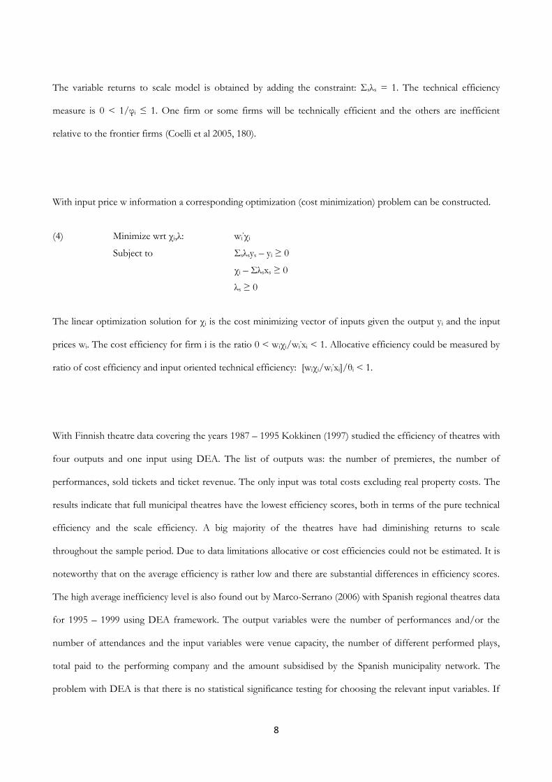
productions is one of the goals set by the state, the following table 9 presents the summary statistics of the DEA

efficiency scores using that output (repertoire, y2).

23

output = y2 VRS, i VRS, o CRS, i CRS, o NRS, i NRS, o

Minimum 0.767 0.180 0.168 0.168 0.168 0.180

Maximum 1 1 1 1 1 1

Mean 0.931 0.766 0.703 0.704 0.703 0.713

Table 9 Summary statistics of DEA efficiency scores, input (i) or output (o) oriented, Variable (VRS), Constant (CRS) or Nonincreasing (NRS) returns to scale, output = y2, n = 46

The efficiency scores using alternative specifications are correlated (table in the appendix). The variable returns

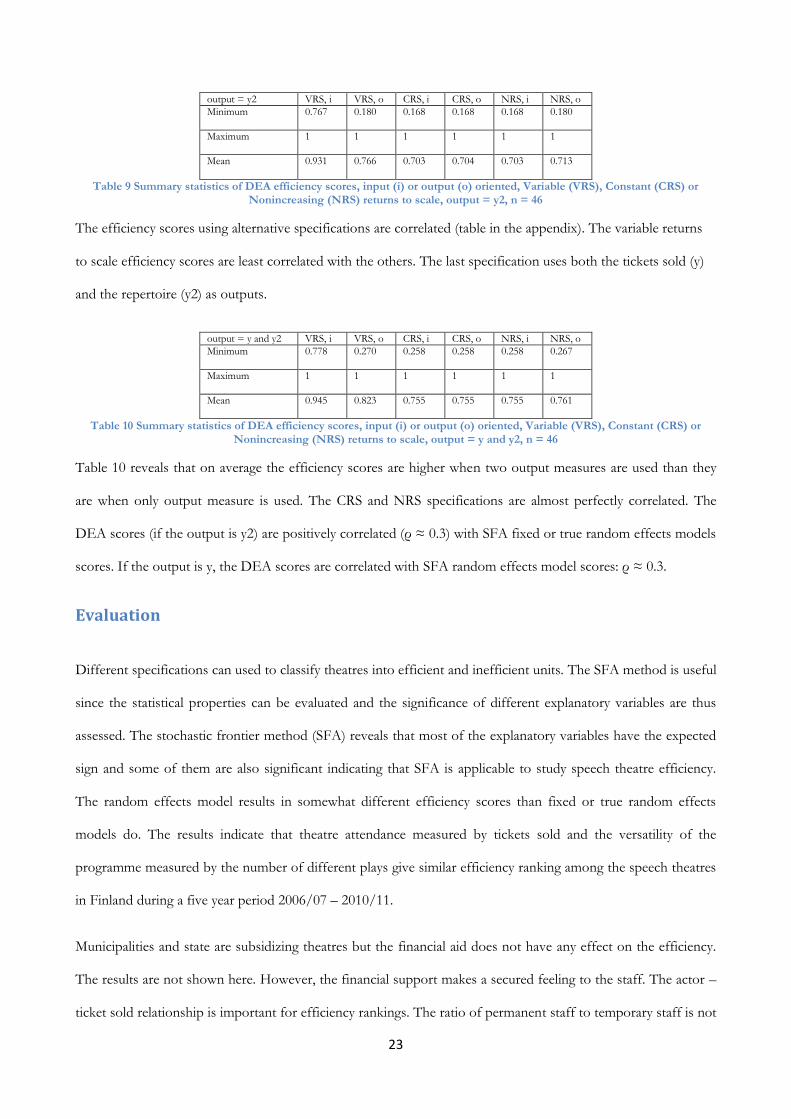
to scale efficiency scores are least correlated with the others. The last specification uses both the tickets sold (y)

and the repertoire (y2) as outputs.

output = y and y2 VRS, i VRS, o CRS, i CRS, o NRS, i NRS, o

Minimum 0.778 0.270 0.258 0.258 0.258 0.267

Maximum 1 1 1 1 1 1

Mean 0.945 0.823 0.755 0.755 0.755 0.761

Table 10 Summary statistics of DEA efficiency scores, input (i) or output (o) oriented, Variable (VRS), Constant (CRS) or Nonincreasing (NRS) returns to scale, output = y and y2, n = 46

Table 10 reveals that on average the efficiency scores are higher when two output measures are used than they

are when only output measure is used. The CRS and NRS specifications are almost perfectly correlated. The

DEA scores (if the output is y2) are positively correlated (ρ ≈ 0.3) with SFA fixed or true random effects models

scores. If the output is y, the DEA scores are correlated with SFA random effects model scores: ρ ≈ 0.3.

Evaluation

Different specifications can used to classify theatres into efficient and inefficient units. The SFA method is useful

since the statistical properties can be evaluated and the significance of different explanatory variables are thus

assessed. The stochastic frontier method (SFA) reveals that most of the explanatory variables have the expected

sign and some of them are also significant indicating that SFA is applicable to study speech theatre efficiency.

The random effects model results in somewhat different efficiency scores than fixed or true random effects

models do. The results indicate that theatre attendance measured by tickets sold and the versatility of the

programme measured by the number of different plays give similar efficiency ranking among the speech theatres

in Finland during a five year period 2006/07 – 2010/11.

Municipalities and state are subsidizing theatres but the financial aid does not have any effect on the efficiency.

The results are not shown here. However, the financial support makes a secured feeling to the staff. The actor –

ticket sold relationship is important for efficiency rankings. The ratio of permanent staff to temporary staff is not

24

evaluated here and therefore is not known whether it is better or not to have permanent actors. Sometimes

visiting actors may be have a positive impact on attendance but on the other hand a permanent staff allows

making a longer perspective to repertoire. The number of administrative and technical staff in relation to the

number of actors does not seem to be significant in explaining efficiency. An important finding is that the

average ticket price has an impact on efficiency.

One of the findings here is that Finnish speech theatres are on average not technically efficient since the mean

efficiency score is ranging from 60 to 70 per cent depending on the SFA model used. True random effects model

gives the highest scores. The differences between fixed and random effects models are notable. The true random

effects model separates unobserved firm-specific heterogeneity from inefficiency and therefore this model tends

to underestimate the inefficiency.

25

References

Abbé-Decarroux, François (1994): The perception of quality and the demand for services: Empirical application to the performing arts. Journal of Economic Behavior & Organization, 23, 99-107

Aigner, D. J., C.A.K. Lovell and P. Schmidt (1977): Formulation and Estimation of Stochastic Frontier Production Function Models. Journal of Econometrics, 6, 21-37

Austen-Smith, David (1980): On the impact of revenue subsidies on repertory theatre policy. Journal of Cultural Economics, 1, 9-17

Battesi, G. E. and T.J. Coelli (1988): Production of Firm-Level Technical Efficiencies with a Generalised Frontier Production Function and Panel Data. Journal of Econometrics, 38, 387-399

Baumol, William and William Bowen (1966): Performing Arts. The Economic Dilemma. A Study of Problems Common to Theater, Opera, Music and Dance. The 20th Century Fund.

Charnes, A., W.W.Cooper and E. Rhodes (1978): Measuring the Efficiency of Decision Making Units. European Journal of Operational Research, 2, 429-444

Coelli, Timothy J., D.S. Prasada Rao, Christopher J. O’Donnell and George E. Battese (2005): An Introduction to Efficiency and Productivity Analysis. Second Edition. Springer, New York

DiMaggio, Paul and Kristen Stenberg (1985): Why do some theatres innovate more than others? An empirical analysis. Poetics, 14, 107-122

Ek, Göran (1991a): Jämförelser av teatrarnas produktivitet – en mätning av institutionsteatrarnas ’inre effektivitet’ via icke-parametriska produktionsfronter. PM Statskontoret

Ek, Göran (1991b): Produktivitetsutvecklingen vid institutions-teatrarna i Sverige – icke-parametriskaproduktionsfronter och malmquist-index. PM Statskontoret

Ek, Göran (1994): Att vara (produktiv) eller inte vara? – En mätning av institutionsteatrarnas produktivitetsförändringar med icke-parametriska produktionsfronter or Malmquist-index. In ”Den offentliga sektorns produktivitetsutveckling 1980 – 1992, Bilagor”, PM Statskontoret

Farrell, M.J. (1957): The Measurement of Productive Efficiency. Journal of the Royal Statistical Society, Series A, CXX, Part 3, 253-290

Farsi, Mehdi and Massimo Filippini (2004): Regulation and Measuring Cost-Efficiency with Panel Data Models: Application to Electricity Distribution Utilities. Review of Industrial Organization, 25, 1-19

Farsi, Mehdi, Massimo Filippini and William Greene (2005): Efficiency Measurement in Network Industries: Application to the Swiss Railway Companies. Journal of Regulatory Economics, 28, 69-90

Färe, R., S. Grosskopf and C.A.K. Lovell (1985): The Measurement of Efficiency of Production. Kluwer Academic Publishers, Boston

Globerman, Steven and Sam H. Book (1974): Statistical cost functions for performing arts organizations. Southern Economic Journal, 40, 668-671

Globerman, Steven and Sam H. Book (1977): Consumption efficiency and spectator attendance. Journal of Cultural Economics, 1, 13-32

Gray, Charles M. (1992): Art Costs and Subsidies: The Case of Norwegian Performing Arts. In Cultural Economics, ed. Ruth Towse and Abdul Khakee, p. 267-273

Greene W. H. (1990): A Gamma-distributed Stochastic Frontier Model. Journal of Econometrics, 46, 141-164

Heilbrun, James (2001): Empirical Evidence of a Decline in Repertory Diversity among American Opera Companies 1991/92 to 1997/98. Journal of Cultural Economics, 25, 63-72

26

Hjorth-Andersen, Chr. (1992): Thaliametrics – A Case Study of Copenhagen Theatre Market. In Cultural Economics, ed. Ruth Towse and Abdul Khakee, p. 257-265

Jenkins, Stephen and David Austen-Smith (1987): Interdependent decision-making in non-profit industries: A simultaneous analysis of English provincial theatre. International Journal of Industrial Organization, 5, 149-174

Johnes, Jill (2006): Measuring efficiency: A comparison of multilevel modelling and data envelopment analysis in the context of higher education. Bulletin of Economic Research, 58, 75-104 Kanerva, Anna and Minna Ruusuvirta (2006): Suomalaisen teatterin tulevaisuus teatterintekijöiden ja kuntien silmin. Yhteenveto teatteriselvityksestä. Cuporen julkaisuja 14/2006

Kangas, Anita and Kalevi Kivistö (2011): Kuntien kulttuuritoiminnan tuki- ja kehittämispolitiikka. Selvittäjien Anita Kangas ja Kalevi Kivistö laatima raportti. Opetus- ja kulttuuriministeriön työryhmämuistioita ja selvityksiä 2011:12

Kim, Yangseon and Peter Schmidt (2000): A Review and Empirical Comparison of Bayesian and Classical Approaches to Inference on Efficiency Levels in Stochastic Frontier Models with Panel Data. Journal of Productivity Analysis, 14, 91-118

Kirjavainen, Tanja (2009): Essays on the Efficiency of Schools and Student Achievement. VATT Publications 53. Helsinki

Kokkinen, Arto (1997): Ammattiteattereiden tehokkuus ja tuottavuuden kehitys 1987 – 1995. VATT keskustelunaloitteita 135. Helsinki

Kumbhakar, Subal C. and C. A. Know Lovell (2000): Stochastic Frontier Analysis. Cambridge University Press, Cambridge

Last, Anne-Kathrin and Heike Wetzel (2010): The efficiency of German public theaters: a stochastic frontier analysis approach. Journal of Cultural Economics, 34, 89-110

Marco-Serrano, Francisco (2006): Monitoring managerial efficiency in the performing arts: A regional theatres network perspective. Annals of Operations Research, 145, 167-181

Meeusen W. and J. van der Broeck (1977): Efficiency Estimation from Cobb-Douglas Production Functions with Composed Error. International Economic Review, 18, 435-444

O’Hagan, John and Adriana Neligan (2005): State Subsidies and Repertoire Conventionality in the Non-Profit English Theatre Sector: An Econometric Analysis. Journal of Cultural Economics, 29, 35-57

Pitt, Mark.M. and Lung-Fei Lee (1981): The measurement and sources of technical inefficiency in the Indonesian weaving industry. Journal of Development Economics, 9, 43-64

Report of a committee on the system of statuort state aid granted to theatres (2003). In Finnish (Selvitys teattereiden valtionosuusjärjestelmän toimivuudesta). Opetusministeriön työryhmämuistiota ja selvityksiä 2003: 13

Simar, Léopold and Paul W. Wilson (1998): Sensitivity Analysis of Efficiency Scores: How to Bootstrap in Nonparametric Frontier Models. Management Science, 44, 49-61

Stevenson, R.E. (1980): Likelihood Functions for Generalised Stochastic Frontier Estimation. Journal of Econometrics, 13, 57-6

Suomen Teatteriliitto (2001): Suomalaisten teatterissa käynti, Heinäkuu 2001. Taloustutkimus Oy.

Suomen Teatteriliitto (2004): Suomalaisten teatterissa käynti, Huhtikuu 2004. Taloustutkimus Oy.

Suomen Teatterit ry (2007): Suomalaisten teatterissa käynti. Syys-lokakuu 2007. Taloustutkimus Oy

Taalas, Mervi (1997): Generalised Cost Functions for Producers of Performing Arts – Allocative Efficiences and Scale Economies in Theatres. Journal of Cultural Economics 21, 335-353

Thorsby, David (2000): The Economics of Cultural Policy. Cambridge University Press, Cambridge

Tinfo (Theatre info Finland), statistics (available on http://www.tinfo.fi)

http://www.tinfo.fi/

27

Tobias, Stefan (2003) Kosteneffizientes Theater? Deutsche Bühnen im DEA-Vergleich. Doctoral Dissertation, University of Dortmund.

Werck, Kristien and Bruno Heyndels (2007): Programmatic choices and the demand for theatre: the case of Flemish theatres. Journal of Cultural Economics, 31, 25-41

Werck, Kristien, Mona Grinwis Plaat Stultjes and Bruno Heyndels (2008): Budgetary constraints and programmatic choices by Flemish subsidized theatres. Applied Economics, 40, 2369-2379

Zieba, Marta (2011): An Analysis of Technical Efficiency and Efficiency Factors for Austrian and Swiss Non-Profit Theatres. Swiss Journal of Economics and Statistics, 147. 233-274

Zieba, Marta and Carol Newman (2007): Understanding Production in the Performing Arts: A Production Function for German Public Theatres. Working Paper, Department of Economics, Trinity College, Dublin (available on http://econpapers.repec.org/paper/tcdtcduee/tep0707.htm)

http://econpapers.repec.org/paper/tcdtcduee/tep0707.htm

28

Appendix


Fixed effects


Fixed effects Random effects True random effects; 100 Halton draws

Fixed Random True random effects; 100 Halton


-2.15*** -1.65*** -1.52*** -1.92*** -1.40* -1.37***

y12 / βy1y1 0.0871*** 0.0643*** 0.0613*** 0.0687*** 0.0466 0.0509**


-0.524*** -0.606* -0.353(*) 0.201 -0.0535 0.320

y22 / βy1y1 0.0428(*) 0.0668 0.0615* 0.0288 0.0528 0.0783*

y1y2 / βy1y2 -0.0187 -0.0170 -0.0494


0.411*** 0.330* 0.383*** 0.0534 0.0331 0.0556 0.181 0.0760 0.0928

x22 / β22 -0.0430*** -0.0423*** -0.0357*** -0.0531*** -0.0533*** -0.0433*** -0.0476*** -0.0479*** -0.0394***


-0.198 -0.103 0.0218 0.763*** 0.299 0.526* -0.798** -0.666 -0.419

x32 / β33 -0.0704* -0.0584 -0.0740*** -0.101*** -0.0250 -0.0469(*) -0.0294 -0.0253 -0.0468(*)

x2x3 / β23 -0.0403** -0.0400* -0.0985 -0.0362*** -0.0178 -0.00793 -0.0436*** -0.0357 -0.0148

y1x2 / γ12 -0.0484*** -0.0400* -0.0493*** -0.00187 0.00873 0.00239

y1x3 / γ13 0.112*** 0.0927(*) 0.0819** 0.143*** 0.114 0.107**

y2x2 / γ22 -0.0818*** -0.0921** -0.0902*** -0.105*** -0.115* -0.0990***

y2x3 / γ23 0.140*** 0.152* 0.0815(*) 0.0118 0.0693 0.0107


net incomes / µ2

constant not shown

𝜎

= √𝜎𝑢2 + 𝜎𝑣

2

0.874 =

√0.866𝑢2 + 0.119𝑣

2

(0.0258)***

0.635

= √0.626𝑢2 + 0.106𝑣

2

(0.0982)***

0.119

= √0.077𝑢2 + 0.091𝑣

2

(0.0186)***

0.817

= √0.809𝑢2 + 0.115𝑣

2

(0.0157)***

0.640

= √0.632𝑢2 + 0.106𝑣

2

(0.0791)***

0.102

= √0.000𝑢2 + 0.102𝑣

2

(0.449)

0.811

= √0.803𝑢2 + 0.113𝑣

2

(0.0280)***

0.589

= √0.580𝑢2 + 0.102𝑣

2

0.097

= √0.000𝑢2 + 0.097𝑣

2

(12.116)

𝜆 = 𝜎𝑢/𝜎𝑣 7.282 (1.180)***

5.923 (2.472)*

0.846 (0.620)

7.014 (1.222)***

5.943 (1.901)**

0.000 (0.000)

7.087 (1.281)***

5.711 (2.104)**

0.000 (0.000)


χ2=21.70*** χ2=1.18 χ2=8.86** χ2=10.06** χ2=4.60* χ2=5.26* χ2 = 42.05*** χ2 = 1.95 not

Wald test: β22+ β33 + β23 = 0

χ2=21.78*** χ2=9.55** χ2=26.53*** χ2=44.12*** χ2=5.94* χ2=34.64*** χ2 = 3.08(*) χ2 = 2.46 not

Wald test: γ12+ γ13 = 0

χ2=610.88*** χ2=0.78 χ2=9.85** χ2=1513.05*** χ2=0.68 χ2=0.00 χ2 = 189.15*** χ2 = 0.33 not

The efficiency of theatres in Finland - Myy...

Documents

Transcript of The efficiency of theatres in Finland - Myy...