The Effects of Algorithmic Labor Market Recommendations:

Evidence from a Field Experiment

John J. Horton

Leonard N. Stern School of Business

New York University

March 4, 2016

Abstract

Algorithmically recommending workers to employers for the purpose of recruiting can substan-

tially increase hiring: in an experiment conducted in an online labor market, employers with tech-

nical job vacancies that received recruiting recommendations had a 20% higher fill rate compared to

the control. There is no evidence that the treatment crowded-out hiring of non-recommended can-

didates. The experimentally induced recruits were highly positively selected and were statistically

indistinguishable from the kinds of workers employers recruit “on their own.” Recommendations

were most effective for job openings that were likely to receive a smaller applicant pool.

1 Introduction

The rise of the Internet created a hope among economists and policy-makers that it would lower

labor market search costs and lead to better market outcomes. Evidence for whether this hope was

fulfilled is mixed (Kuhn and Skuterud, 2004; Kuhn and Mansour, 2014), but to date the rise of the In-

ternet seems to have had modest effects on search and matching in the conventional labor market.

However, simply providing parties searchable listings of jobs and resumes—the core functionality

of online job boards—hardly exhausts the possibilities created by marketplace digitization.

In many online product markets, the creating platform now goes beyond simply providing in-

formation but rather makes explicit, algorithmically generated recommendations about whom to

trade with or what to buy (Varian, 2010; Resnick and Varian, 1997; Adomavicius and Tuzhilin, 2005).

Algorithmic recommender systems can try to infer preferences, determine the feasible choice set

and then solve the would-be buyer’s constrained optimization problem. At their best, algorithmic

recommendations can incorporate information not available to any individual party. Furthermore,

these recommendations have zero marginal cost and recommendation quality potentially improves

with scale.

To date, algorithmic recommendations have been rare in labor markets, but as more aspects of

the labor market become computer-mediated, recommendations will become increasingly feasi-

ble. However, it is not clear that labor market recommendations can meaningfully improve upon

what employers can do for themselves. Perhaps choosing who is appropriate for a particular job

opening requires evaluating ineffable qualities that are difficult to capture in a statistical model. Or

1

perhaps assembling a pool of reasonable applicants is simply not that costly to employers. Beyond

the perspective of the individual employer, a concern with recommendations is that, by design, they

encourage an employer to consider some workers but not others. If crowd-out effects are strong—

which has been the case in some job search assistance programs in conventional labor markets

(Crépon et al., 2013)—recommendation interventions are less attractive from a social welfare per-

spective.

In this paper, I report the results of an experimental intervention in which algorithmically gener-

ated recommendations were made to employers about which workers to recruit for their job open-

ings.1 The context for the experiment was oDesk, a large online labor market. On oDesk, employer

recruiting is one of two “channels” employers use to get applicants for their job openings—the other

is to rely on “organic” applicants finding the job listing and applying without prompting by the em-

ployer. Before the experiment, employers could recruit only by searching through listings of workers

and inviting those who looked promising.

I find that when offered algorithmic recommendations, a large fraction of employers follow

them: the treatment increased the fraction of employers recruiting by nearly 40%. Recruited work-

ers accepted invitations and applied for the associated job at the same rates in both the treatment

and control groups. As such, the treatment substantially increased the number of recruited appli-

cants in the applicant pools of treated employers.

Recruited applicants were highly positively selected in terms of market experience and past

earnings. This characterization held in both the treatment and control groups—experimentally in-

duced recruits “looked like” the kinds of workers employers recruit on their own. Employers showed

a strong preference for screening recruited applicants relative to non-recruited organic applicants,

but this difference did not depend on the treatment assignment. This lack of a difference across ex-

perimental groups undercuts the notion that employers believed that recommended workers were

better or worse than their observable characteristics suggested.

Being offered recruiting assistance raised the probability that an employer hired someone for

her job opening, but not for all types of job openings: the treatment increased the overall fill rate in

technical job openings by 20%, but had no detectable effect on non-technical job openings.2 The

strong effects on technical job openings do “show up” in the entire sample, in that the treatment

substantially raised the probability that the wage bill for a job opening exceeds $500 (technical job

openings, when filled, lead to projects that are, on average, larger than non-technical projects in

terms of wage bill).

There are several potential reasons for why the treatment was only effective for technical job

openings, but the most likely explanation is that: (1) technical job openings attract fewer organic

applicants, which are substitutes for recruited applicants, and (2) employers with technical open-

ings seem to value experience and are less cost-sensitive than their non-technical counter-parts—

and recruited applicants tend to be both more experienced and more expensive. Highlighting the

importance of the organic applicant count in explaining treatment effect heterogeneity, when the

treatment is conditioned on the expected number of organic applicants to a job opening, I find that

the technical/non-technical distinction is largely explained by differences in applicant pool size:

the treatment is more effective for jobs expected to receive few applicants than for jobs expected to

1I use the term “employer” throughout the paper for consistency with the extant labor literature rather than as a commentary

on the precise nature of the contractual relationship between parties on the platform.2Throughout the paper, I refer to employers as “she” and applicants/workers as “he.”

2

receive many applicants.

Despite raising the fill rate for technical job openings, there is no evidence of crowd-out of

organic applicants for those job openings. The likely explanation is that the low hire rate—less

than 50% of job openings are filled—creates “space” to increase hiring without crowd-out. Those

matches that were formed in the treatment group were indistinguishable from matches in the con-

trol group with respect to match outcomes, such as the total wage bill and feedback score. However,

the study is underpowered to detect even fairly large changes in match quality.

To summarize, the evidence is most parsimoniously explained by the following: (1) employers

acted upon the recommendations because it was cheap to do so and the recommended candidates

were similar to the kind of workers they would have recruited themselves—namely relatively high-

cost but high-quality applicants; (2) recommendations were effective at raising fill rates for tech-

nical job openings because these employers have relatively high returns to additional high-quality

applicants; (3) where they were effective, recommendations had little crowd-out because the base-

line vacancy fill rate was low enough that market expansion effects could dominate.

The main implication of the paper is that a relatively unsophisticated algorithmic recommender

system—unsophisticated compared to what oDesk (now known as “Upwork”) does presently—can

substitute for some of the work employers have to do when filling a job opening, and this substitu-

tion can substantially increase hiring. However, the paper also highlights the economic nature of

the employer’s hiring problem; recommendation efficacy turned out to depend less on the details

of the recommendation algorithm—at least in terms of the kinds of recruits it generated—and more

in how employers valued recruited applicants and how many organic applicants they could expect

to receive in the absence of recommendations.

Although we can imagine algorithms that might improve match quality—some standardized

job tests, which are a kind of algorithm for hiring seem successful at doing so—the algorithm used

in this paper worked primarily by expanding the pool of potential applicants by lowering the em-

ployer’s costs of assembling such a pool.

This intervention was conducted in a setting where search costs are presumably quite low: oDesk

is information rich, in that both sides have access to the universe of job seekers and job openings,

and at every step, both sides have comprehensive data on past job histories, wages, feedback scores

and so on. In this environment, one might suppose that the marginal benefit of algorithmic recom-

mendations would be low, and yet this is strongly not the case. In conventional settings where the

stakes are higher, one might expect employers to expend more effort in recruiting and screening,

but this implies that the opportunity for reducing costs is even greater, even if the expected benefits

in terms of match formation might be lower.

2 Empirical Context

During the last ten years, a number of online labor markets have emerged. In these markets, firms

hire workers to perform tasks that can be done remotely, such as computer programming, graphic

design, data entry, research and writing. Markets differ in their scope and focus, but common ser-

vices provided by the platforms include maintaining job listings, hosting user profile pages, arbi-

trating disputes, certifying worker skills and maintaining feedback systems. The experiment in this

paper was conducted on oDesk, the largest of these online labor markets.

In the first quarter of 2012, $78 million was spent on oDesk. The 2011 wage bill was $225 million,

3

representing 90% year-on-year growth from 2010. As of October 2012, more than 495,000 employers

and 2.5 million freelancers have created profiles, though a considerably smaller fraction are active

on the site. Approximately 790,000 job openings were posted in the first half of 2012. See Agrawal et

al. (2013a) for additional descriptive statistics on oDesk.

Based on dollars spent, the top skills in the marketplace are technical skills, such as web pro-

gramming, mobile applications development (e.g., iPhone and Android) and web design. Based

on hours worked, the top skills are web programming again, but also data entry, search engine op-

timization and web research, which are non-technical and require little advanced training. The

difference in the top skills based on dollars versus hours reflects a fundamental split in the market-

place between technical and non-technical work. There are highly skilled, highly paid freelancers

working in non-technical jobs, yet a stylized fact of the marketplace is that technical work tends to

pay better, generate longer-lasting relationships and require greater skill.

There has been some research which focuses on the oDesk marketplace. Pallais (2014) shows

via a field experiment that past worker experience on oDesk is an excellent predictor of being hired

for subsequent work on the platform. Stanton and Thomas (2012) use oDesk data to show that

agencies (which act as quasi-firms) help workers find jobs and break into the marketplace. Agrawal

et al. (2013b) investigate what factors matter to employers in making selections from an applicant

pool and present some evidence of statistical discrimination; the paper also supports the view of

employers selecting from a more-or-less complete pool of applicants rather than serially screening.

2.1 Job posting, recruiting, screening and hiring on oDesk

The process for filling a job opening on oDesk is qualitatively similar to the process in conventional

labor markets. First, a would-be employer on oDesk creates a job post: she writes a job title and

describes the nature of the work, chooses a contractual form (hourly or fixed-price) and specifies

what skills the project requires (both by listing skills and choosing a category from a mutually exclu-

sive list) and what kinds of applicants she is looking for in terms of past experience. Employers also

estimate how long the project is likely to last. Once their job post is written, it is reviewed by oDesk

and then posted to the marketplace.

Once posted to the marketplace, would-be job applicants can view all the employer-provided

job post information. Additionally, oDesk also presents verified attributes of the employer, such

as their number of past jobs, average paid wage rate and so on. When a worker applies to a job

opening, he offers a bid (which is an hourly wage or a fixed price, depending on contract type) and

includes a cover letter. After applying, the applicant immediately appears in the employer’s ATS,

or “applicant tracking system.” The employer can view an applicant’s first name, profile picture,

offered bid and a few pieces of other oDesk-verified information, such as hours worked and his

feedback rating from previous projects (if any). Employers can click on a worker’s application to

view his full profile, which has that worker’s disaggregated work history, with per-project details on

feedback received, hours worked and earnings. As these clicks are recorded by oDesk, they provide

an intermediate measure of employer interest in a particular applicant.

Although all job applications start with the worker applying to a job opening, not all of these

applications are initiated by the worker: as in conventional labor markets, employers on oDesk may

choose to recruit candidates to apply for their jobs. Employer recruiting on oDesk begins with the

employer searching for some skill or attribute she is looking for in candidates; the search tools on

4

oDesk will return lists of workers and will contain information about that worker’s past work history.

The employer can “invite” any worker she is interested in recruiting. These recruiting invitations are

not job offers, but rather invitations to apply to the employer’s already-posted job opening. As will

become evident, these recruited applicants tend to be highly positively selected: they have more

experience, higher past wages, greater earnings etc., and consequently, also bid considerably more

for hourly jobs than non-recruited organic applicants.

Of course, recruited workers are not required to apply to the job opening—only about half do

apply. Those who do apply appear in the employer’s ATS alongside whatever organic applicants

the job opening has attracted. Employers are free to evaluate candidates at any time after they

post their jobs. Presumably different employers use different approaches to evaluate applicants

depending upon their urgency in filling the job opening and the fixed costs of a screening “session.”

Anecdotally, some employers screen applicants as they arrive, while others wait to process them in

batch, after a suitable number have arrived.

Although employers can recruit at any time, employers generally recruit shortly after posting

their job openings, before they receive any organic applicants. If recruiting is costly, a natural ques-

tion is why would employers ever recruit “ex ante,” i.e., before receiving organic applicants? One

reason is that it allows the employer to obtain a better applicant pool more quickly, and given that

most employers want to fill their job openings as soon as possible, ex ante recruiting can be rational.

Ex ante recruiting also allows employers to evaluate candidates “in batch” by assembling a more or

less complete pool of applicants first and then screening them all at once.

If the employer makes a hire, oDesk intermediates the relationship. If the project is hourly, hours

worked are measured via custom tracking software that workers install on their computers. The

tracking software, or “Work Diary,” essentially serves as a digital punch clock, allowing hours worked

and earnings to be measured essentially without error.

The oDesk marketplace is not the only marketplace for online work (or IT work more generally).

As such, one might worry that every job opening on oDesk is simultaneously posted on several

other online labor market sites and in the conventional market. If this were the case, it would make

interpreting events happening on oDesk more complex, particularly for an experiment focused on

raising the number of matches formed; perhaps any observed increase in the fill rate simply came

at the expense of some other marketplace which is unobserved.

Despite the possibility of simultaneous posting, survey evidence suggests that online and offline

hiring are only very weak substitutes and that “multi-homing” of job openings on other online labor

markets is relatively rare. When asked what they would have done with their most recent project if

oDesk were not available, only 15% of employers responded that they would have made a local hire.

In this same survey, online employers report that they are generally deciding among (a) getting the

work done online, (b) doing the work themselves and (c) not having the work done at all. The survey

also found that 83% of employers said that they listed their last job job openings on oDesk alone.

This self-report appears to be credible, as Horton (2015) found limited evidence of multi-homing

when comparing jobs posted on oDesk and its largest (former) rival, Elance. This limited degree of

multi-homing narrows the scope of potential crowd-out effects from marketplace interventions to

those happening within the platform rather than across platforms.

5

3 Description of the experiment

In June 2011, oDesk launched an experimental feature that targeted new employers, with “new” de-

fined as those who had not previously posted a job opening on oDesk. Immediately after posting

a job opening, a treated employer was shown up to six recommended workers that the employer

could recruit to apply for her job opening. Control employers received the status quo experience of

no recommendations. The total sample for the experiment consisted of 6,209 job openings, which

is the universe of job openings that were posted by new employers during the experimental pe-

riod and for which recommendations could be made (regardless of treatment assignment). The

randomization was effective and the experimental groups were well balanced (see Appendix A for

details).3

The actual recommendations were delivered to treated employers via a pop-up interface, a

screen-shot of which is shown in Figure 1. From this interface, the employer could compare each

recommended worker’s photograph, listed skills, average feedback score and stated hourly wage. If

the employer clicked on a worker’s application in the ATS, she could see that worker’s country, total

hours worked on the platform, passed skills tests, past employer evaluations and other pieces of

potentially match-relevant information. Employers could choose to invite any number of the rec-

ommended workers to apply for their jobs (including no one at all). Once a treated employer closed

the recommendations pop-up window, she experienced the same interface and opportunities as

employers in the control group.

Recommendations were made based on the fit of a statistical model using historical oDesk hir-

ing data. The model incorporated measures of worker relevance to the job in question, the worker’s

ability and the worker’s availability, i.e., capacity to take on more work. Relevance was measured

by the degree of overlap in the skills required for the job opening and the skills listed by the worker

in his profile. Ability was defined as a weighted sum of his skill test scores, feedback ratings and

past earnings. Availability was inferred from signals such as the worker recently ending a project or

applying to other job openings. If the employer invited a recommended worker, the experience of

the invited worker and employer were from then on identical to what would have happened had the

employer simply found and invited that worker on her own. The invited worker did not know that

their invitation was experimentally induced, nor was the employer later notified of that worker’s

invited status in the ATS.

One unfortunate limitation of the design of the experiment was that the identity of workers who

were recommended (or would have been recommended in the control) was not logged. For some

outcomes of interest, such as the overall job fill rate, not having access to the individual recom-

mendations is irrelevant. However, for other questions, such as whether recommendations were

“better” in some categories of work, not having the actual recommendations is a limitation. As a

work-around, it is possible to make a reasonable inference about which invitations and follow-on

applications were more likely to be experimentally induced: because recommendations were pre-

sented as a pop-up immediately after a job opening was posted, recruiting invitations made shortly

after the posting were more likely to be caused by the treatment. For analyses where it is useful

to identify experimentally induced invitations and applications, I define “ex ante” recruiting as re-

cruiting that occurred within the first hour after the associated job opening was posted.

3This appendix also discusses the possibility of cross-unit effects i.e., violations of the SUTVA assumption and discusses why,

given the size of the experiment relative to the market as a whole, such concerns are likely unwarranted.

6

Figure 1: Recommendations shown to treated employers after posting their job openings

Notes: This figure shows the interface presented to employers in the treatment group. It displays

a number of recommended workers with good on-platform reputations, skills relevant to the

employer’s job opening and predicted availability for the employer’s project.

7

4 Conceptual framework and related work

An employer’s search and screening process could benefit from an algorithmic approach in several

ways. For example, an algorithm could be used to help evaluate an already-assembled pool of can-

didates. Using “algorithms” to screen candidates has a long (uncomputerized) history: standard-

ized exams, like those used for entrance into a civil service, take applicant characteristics—namely

their answers to exam questions—and returns a recommendation about whom to hire.4 Informa-

tion technology has made this kind of test-based screening easier, as it simplifies administration

and grading: Autor and Scarborough (2008) describes a large national retail chain switching from

an informal screening process to a standardized testing procedure, finding that the move increased

productivity and increased tenure at the firm. Hoffman et al. (2015), looking at the staggered in-

troduction of pre-employment testing also find that testing improves match quality and tenure.

Furthermore, those managers exercising discretion—over-ruling the algorithm—end up with sys-

tematically worse outcomes.

Another use of algorithms could simply be to identify and deliver “reasonable” applicants for a

job opening who the employer could then recruit, at her discretion. The algorithm could do a better

or worse job than a firm’s unassisted search efforts could accomplish, with algorithm performance

ranging from (a) a random sample of candidates in the market to (b) the precise applicants, out

of all possible applicants, that would make the best matches if hired. Interestingly, even a random

sample might be valuable, as a perennial concern in labor markets is that those actively looking for

work are adversely selected (such as through the mechanism in Gibbons and Katz (1991)). A sample

of potential recruiting targets might be especially welcome in labor markets where parties generally

have not had ready access to the whole pool of potential workers.

The experiment described in this paper was intended to increase the applicant pool size, with

the hope that the recommendations would be good enough that the employer would not simply

discard them. As such, the experiment was most conceptually similar to active labor market policies

in which a government agency assists with job-finding, with the focus in these programs typically

on helping workers. These programs tend to have positive, albeit modest, effects on employment

probability (Kluve, 2010; Card et al., 2010). However, a perennial concern with such programs is

that the benefits mainly come at the expense of those not assisted. This concern is highlighted by

Gautier et al. (2012) and was recently illustrated by Crépon et al. (2013), which was a large-scale job-

finding assistance program that seemed to “work” mostly by displacing non-assisted job seekers.

The labor market intervention in this paper was demand-focused, with assistance offered to

employers. As such, understanding how these assistance might help requires a model of employer

search and screening. Unfortunately, there is relatively little research in economics on how em-

ployers fill job openings and thus little guidance on how worker-finding assistance should affect

outcomes (Oyer and Schaefer, 2010). Most of the literature on labor market search has focused

on workers searching for jobs, not firms searching for workers. An exception is Barron and Bishop

(1985), which finds that employers with hard-to-fill job openings or those that require more training

report screening larger pools of applicants and screening each applicant more intensively. Pelliz-

zari (2011) finds that more intensive recruitment by a sample of British employers is associated with

better-quality matches. The resultant matches pay more, last longer and lead to greater employer

satisfaction, though the direction of causation is not clear.

4The Chinese civil service examination system dates back to the mid 600s.

8

Existing models of employer search are similar to simple job search models e.g., Burdett and

Cunningham (1998); Barron et al. (1989); Barron and Bishop (1985); firms serially screen applicants

who arrive over time without recall; firms hire the first applicant above some “reservation value” for

the position. These models are hard to map to key empirical features of the oDesk domain, such as

the decision whether or not to recruit and whether the treatment would have heterogeneous effects

based on the nature of the job opening. Furthermore, as van Ours and Ridder (1992) points out,

there is little empirical basis for this sequential search-based view of hiring; they find that “almost all

vacancies are filled from a pool of applicants that is formed shortly after the posting of the vacancy.”

Given the difficulty of mapping existing employer search models to the current domain, I de-

velop a simple model more closely tied to the empirical context and which can help interpret the

experimental results. Some of the modeling choices are motivated by the experimental results, so

the empirical results should not be interpreted as ex post tests of the model. Rather, the model is

intended to offer one way of framing what the experimental intervention did and see if the various

empirical results can at least be rationalized by a simple model.

I model the employer’s decision about recruiting intensity as her weighing the cost of recruiting

versus the benefit from recruiting in terms of a better applicant pool and thus a higher probability

of filling her job. I consider how a change in the cost of recruiting affects the extent of employer

recruiting and the probability that a job opening is filled; a focus is on whether differences in organic

applicant counts leads to heterogeneous treatment effects. I also characterize how a reduction in

recruiting costs affects the probability that a non-recruited applicant is hired (which speaks directly

to the crowd-out question).

4.1 The employer’s recruiting and hiring problem

A firm is trying to produce some output, y , that will yield py in the product market when sold.

The firm knows that it will get a collection of A organic applicants for sure. It can also recruit R

applicants, at a cost of cR. Both kinds of workers are ex ante homogeneous,5 but each worker varies

in how good of a “fit” he is for a particular job and thus how likely he is to produce the output. The

firm has to pay a hired worker the market wage of w .

Once a worker applies, the firm observes y , which is the firm’s unbiased estimate of the prob-

ability that the worker can produce the output. Assume that y ∼ U [0,1]. To keep things simple, I

assume that the firm only has the time and capacity to screen one and only one applicant and that

the pay-off to hiring is large enough that screening the top candidate is always worthwhile. The firm

selects the applicant with the highest predicted productivity, y∗, and puts him through additional

screening to see if he can actually produce the output. As the firm’s estimates are unbiased, the

probability that the firm makes a hire following this additional screening is

Pr {Hire|y∗} = y∗; (1)

with probability 1− y∗ the firm hires no one. The firm’s screening technology is perfect, and so a

hired worker can produce the output with certainty.

5This homogeneity assumption is counter-factual in the actual data—recruited candidates tend to be highly positively

selected—but this fact does not change the essential features of the firm’s recruiting problem. However, accounting for it in

a model would substantially increase model complexity.

9

The expected productivity of the top applicant, conditioned upon having an applicant pool of

size A+R is

E[y∗|A,R] =

∫1

0(A+R)y A+R−1d y =

A+R

A+R +1. (2)

The firm’s recruiting optimization problem is thus

maxR

(p −w)E[y∗|A,R]− cR (3)

and the first-order condition is p −w = (A+R +1)2c, so the interior solution is

R∗=

√(p −w)/c −1− A. (4)

The optimal recruiting solution has appealing comparative statics: there is more recruiting

when recruiting is cheaper and more recruiting when the profit earned from producing the out-

put is greater. As one would expect given that there is nothing special about recruits, the number of

organic applicants, A, enters linearly, with a unit coefficient in Equation 4, implying that an increase

of one additional organic applicant would cause the firm to want to decrease recruited applicants

by exactly one. If A is sufficiently large, a corner solution would result, with R∗ = 0.

If c is exogenously lowered, such as by a third party making recruiting recommendations, then

R∗ goes up, as

∂R∗

∂c=

∂

∂c

[√(p −w)/c

]< 0. (5)

Note that the effect on R∗ from a small change in c does not depend on A, but rather only p−w and

c. The effect of more recruits on the probability a hire is made is

∂y∗

∂R=

1

(A+R +1)2> 0. (6)

When R increases, y∗ increases, and thus more hires are observed. However, this increase in the

hire probability from more recruits is declining in the number of organic applicants, as

∂

∂A

[∂y∗

∂R

]=−

2

(A+R +1)3< 0. (7)

For job openings with a lower A, the effect of a lower c will have a larger effect on hiring probabilities

than in job openings with a higher A. The change in the probability of a hire is

∂y∗

∂c=

∂y∗

∂R∗

∂R∗

∂c. (8)

In terms of crowd-out, the expected number of hired organic applicants per job opening is

A/(A +R)y∗, which is just the fraction of applicants who are organic times the fill probability, y∗.

The change in this expectation from a change in c, is

∂(Pr {hired organic applicant})

∂c=−

A

(A+R)2y∗∂R∗

∂c. (9)

The gross amount of crowd-out of organic applicants caused by a reduction in c is the change in

recruiting, scaled by the base hire rate.6

6Note that the envelope theorem allows us to ignore the marginal jobs that are induced to fill by the treatment.

10

5 Results

In the language of the model presented above, an interpretation of the recommendations treatment

was that it lowered c, the cost of recruiting. In the model, a lowered cost of recruiting should increase

recruiting and raise the probability that a hire is made, though the size of the treatment effect on

the hire rate depends on the number of organic applicants.

Many of the experimental results are apparent in a simple comparison of outcome means across

the treatment and control groups: Table 1 reports the fraction of employers that recruited, made a

hire, and ultimately spent more than $500 against their job opening, by experimental group. The

“made a hire” outcome is further decomposed into an indicator for whether the employer hired

a recruited applicant or an organic applicant. The top panel of the table uses all job openings as

the sample, while the middle and bottom panels show results for non-technical and technical job

openings, respectively.

Table 1: Outcome means by experimental groups

Treatment

mean:

XT RT

Control mean:

XC T L

Difference in

means:

XT RT − XC T L

p-value

Outcomes for All Vacancies

Recruited 0.207 (0.007) 0.148 (0.006) 0.059 (0.010) <0.001 ***

Made a hire 0.295 (0.008) 0.276 (0.008) 0.019 (0.011) 0.102

Hired an organic applicant 0.272 (0.008) 0.266 (0.008) 0.006 (0.011) 0.592

Hired recruited applicant 0.048 (0.004) 0.040 (0.003) 0.009 (0.005) 0.097 †

Wage bill > $500 0.072 (0.005) 0.058 (0.004) 0.014 (0.006) 0.023 *

Outcomes for Non-Technical Vacancies

Recruited 0.199 (0.010) 0.153 (0.009) 0.045 (0.014) 0.001 ***

Made a hire 0.331 (0.012) 0.339 (0.012) -0.008 (0.017) 0.630

Hired an organic applicant 0.311 (0.012) 0.323 (0.012) -0.012 (0.017) 0.476

Hired recruited applicant 0.045 (0.005) 0.047 (0.005) -0.003 (0.008) 0.730

Wage bill > $500 0.059 (0.006) 0.049 (0.005) 0.009 (0.008) 0.254

Outcomes for Technical Vacancies

Recruited 0.216 (0.011) 0.143 (0.009) 0.073 (0.014) <0.001 ***

Made a hire 0.259 (0.011) 0.216 (0.010) 0.043 (0.015) 0.005 **

Hired an organic applicant 0.233 (0.011) 0.212 (0.010) 0.022 (0.015) 0.146

Hired recruited applicant 0.052 (0.006) 0.032 (0.004) 0.020 (0.007) 0.006 **

Wage bill > $500 0.085 (0.007) 0.066 (0.006) 0.019 (0.009) 0.040 *

Notes: This table reports outcome means and standard errors across experimental groups from the recommendations ex-

periment. In the experiment, the treatment group of employers received algorithmically-generated recommendations of

candidates for their vacancies while the control group did not. The unit of randomization was the posted vacancy. The

standard error for each calculated mean is in parentheses next to the estimate. The top panel means are calculated using all

observations. The middle panel uses only non-technical vacancies, while the bottom panel uses only technical vacancies.

Reported p-values are the for two-sided t-tests of the null hypothesis of no difference in means across groups. “Recruited” is

an indicator for whether the employer made an invitation to a worker within 1 hour of posting their job. “Filled vacancy” is

an indicator for whether the employer hired a worker and spent more than $1. A “recruited applicant” is one one that applied

to the vacancy after being recruited by the employer, whereas an organic applicant is one who applied without prompting

by the employer. The “wage bill” is the total amount spent by the employer against that vacancy. Significance indicators:

p ≤ 0.10 : †, p ≤ 0.05 : ∗, p ≤ 0.01 : ∗∗ and p ≤ .001 : ∗∗∗.

11

The key experimental results are that: (1) the treatment increased recruiting among all job open-

ings; (2) experimentally induced recruited applicants were similar on observables to the workers

that employers recruit on their own; (3) the treatment increased fill rates among technical job open-

ings only; (4) where recommendations were effective, there was no observable reduction in hiring

of non-recommended organic applicants. These results are explored in more depth in the sub-

sections that follow. The effects of the treatment on match quality are presented in Appendix B due

to space considerations. The main conclusion from Appendix B is that within the limits of statisti-

cal power available, there is no difference across experimental groups on match outcomes such as

feedback and the total wage bill.

5.1 Employer ex ante recruiting

The treatment was designed to increase employer recruiting. Table 2 shows that this goal was

achieved for all categories of work, with recruiting increasing substantially among treated employ-

ers. There is no evidence that the treatment increased ex post recruiting, i.e., recruiting that oc-

curred more than one hour after the job opening was posted, undercutting the notion that the

treatment may have worked simply by alerting the employer to the possibility of recruiting. The

treatment appears to have worked primarily on the extensive margin (i.e., increasing the number of

employers recruiting at all) rather than intensive margin (i.e., the number of candidates recruited,

conditional upon recruiting).

Column (1) of Table 2 reports an estimate of

EMPRECRUITED j =β0 +β1TRT j +ǫ, (10)

where EMPRECRUITED j is an indicator for whether the employer recruited ex ante and TRT j is

whether the employer received the recommendations treatment. The treatment increased ex ante

recruiting by about 6 percentage points, from a base of only about 15 percentage points.

To test whether the treatment differed by the nature of the work, Column (2) reports an estimate

of

EMPRECRUITED j =β0 +β1TRT j +β2TECH j +β3

(TRT j ×TECH j

)+ǫ, (11)

where TECH j is an indicator for whether the job opening was technical. The coefficient on the in-

teraction term is positive and potentially economically significant—uptake was about 3 percentage

points higher for technical job openings—but the coefficient is not statistically significant.

If the treatment “worked” by simply alerting employers to the possibility of recruiting, then the

treatment might have a positive effect on ex post recruiting. However, this does not appear to be

the case. In Column (3), the outcome is an indicator for whether the employer sent any ex post

recruiting invitations, which I define as all invitations sent after the first hour of job posting. The

coefficient is negative, small in magnitude and precisely estimated.

In addition to measuring recruiting as a binary measure, I also examine the effect of the treat-

ment on the count of recruited applicants. Column (4) reports a regression where the dependent

variable is the number of ex ante recruits per job opening. The coefficient on the treatment is posi-

tive and highly significant, with the treatment increasing the count of recruits from a base of about

a third of an ex ante recruit per opening to nearly half an ex ante recruit per opening. Note that for

12

Table 2: Effects of the recommendations treatment on employer ex ante recruiting

Measures of employer recruiting:

Any ex ante? Any ex post? Num. ex ante

COP

(1) (2) (3) (4) (5)

Assigned to Treatment (TRT) 0.059∗∗∗ 0.045∗∗∗ −0.004 0.151∗∗∗ 0.094

(0.010) (0.014) (0.008) (0.032) (0.135)

Technical vacancy (TECH) −0.010

(0.013)

TRT × TECH 0.028

(0.019)

Constant 0.148∗∗∗ 0.153∗∗∗ 0.124∗∗∗ 0.332∗∗∗ 2.384∗∗∗

(0.006) (0.009) (0.006) (0.020) (0.100)

Sample Num Recruits > 1? N N N N Y

Sample Num Recruits < 11? N N N Y Y

Observations 6,209 6,209 6,209 6,127 1,018

R2 0.006 0.006 0.00003 0.004 0.0005

Notes: This table reports OLS regressions where the dependent variable is some measure of recruiting. The same sample is

used in both Columns (1) and (2), and it consists of all job openings assigned to the recommendations experiment. Ex ante

recruiting is the employer recruiting within the first hour after posting a job opening. “Treatment” is an indicator that the

employer received recommendations about candidates to recruit. “Technical” is an indicator for that opening requiring com-

puter programming. The Column (3) outcome is an indicator for any ex post recruiting (i.e., recruiting after the first hour of

a job posting). In Column (4) the outcome is the count of ex ante recruiting invitations, but with the sample restricted to job

openings sending 10 or fewer of these invitations. Column (5) has the same outcome, but with the sample further restricted to

those employers sending at least one ex ante recruiting invitation. Robust standard errors are reported. Significance indicators:

p ≤ 0.10 : †, p ≤ 0.05 : ∗, p ≤ 0.01 : ∗∗ and p ≤ .001 : ∗∗∗.

13

this estimation, the sample is restricted to job openings with ten or fewer ex ante recruiting invita-

tions, in order to improve the precision of the estimates. (A small number of employers send very

large numbers of recruiting invitations.)

In the Column (5) regression, the sample is further restricted to job openings where the em-

ployer sent at least one ex ante recruiting invitation. This allows me to test whether the treatment

increased the number of recruits, conditional upon recruiting at least one recruit. Although the co-

efficient on treatment indicator is positive, it is not significant and is small in magnitude relative

to the baseline count in the control, which is a little less than two and a half ex ante recruits per

opening.

The main effect of the treatment was to cause firms to go from “not recruiting” to “recruiting,”

rather than increasing the count of recruits among employers who would have recruited anyway.

As confirmation of this, taking the 6 percentage point increase on the extensive margin (taken from

Column (1)) and multiplying it by the control group conditional-on-positive number of ex ante re-

cruits, which is 2.4, the expected increase in the count of recruits is 0.156, which is close to the

realized increase of 0.151 (from the coefficient on the treatment indicator in Column (4)).

5.2 Responses from recruited workers to ex ante recruiting invitations

A primary practical concern with algorithmically generated recommendations is their “quality,”

which we might think of as their usefulness to employers and workers alike. One proxy measure of

recommendation quality is the discretion invited workers show when responding: workers would

presumably respond more negatively to worse invitations (or invitations from worse employers).

Using the sample of ex ante recruiting invitations, Table 3 shows that there is no evidence that work-

ers respond differently to recruiting invitations likely to have been experimentally induced, relative

to the control group, suggesting that those experimentally induced invitations are similar to the

“natural” invitations sent in the control group.

First, I examine whether the invited worker responded at all to the invitation, either to accept or

reject. Column (1) of Table 3 reports an estimate of

RESPONDi j =β0 +β1TRT j +ǫ j (12)

where RESPONDi j is an indicator for whether the recruited worker i responded to the recruiting

invitation to apply to job opening j , either yes or no (RESPONDi j = 0 would mean that the recruited

worker ignored the invitation). The sample is all ex ante recruiting invitations where the employer

sent ten or fewer ex ante recruiting invitations in total.7 To account for the hierarchical nature

of the data, standard errors are clustered at the level of the job opening. There is no evidence of

systematic difference across experimental groups with respect to recruited worker responsiveness;

the coefficient on the treatment indicator in Column (1) is very close to zero, with a small standard

error (slightly less than 2 percentage points).

Next I look at whether the invited worker actually accepted the recruiting invitation. In Columns (2)

and (3), the dependent variable is whether the recruited worker accepted the invitation by submit-

ting an application to the associated job opening. Column (2) shows that there is no evidence of

7I remove employers sending many invitations because they are more akin to spammers rather than bona fide employers.

Further, by using an OLS model but then clustering standard errors to account for the hierarchical nature of the data, including

“mass-invite” employers unduly weights their actions in the point estimates.

14

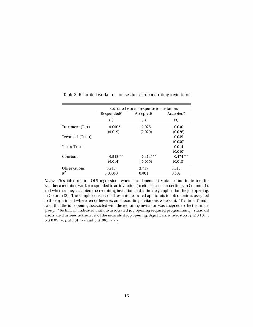
Table 3: Recruited worker responses to ex ante recruiting invitations

Recruited worker response to invitation:

Responded? Accepted? Accepted?

(1) (2) (3)

Treatment (TRT) 0.0002 −0.025 −0.030

(0.019) (0.020) (0.026)

Technical (TECH) −0.049

(0.030)

TRT × TECH 0.014

(0.040)

Constant 0.588∗∗∗ 0.454∗∗∗ 0.474∗∗∗

(0.014) (0.015) (0.019)

Observations 3,717 3,717 3,717

R2 0.00000 0.001 0.002

Notes: This table reports OLS regressions where the dependent variables are indicators for

whether a recruited worker responded to an invitation (to either accept or decline), in Column (1),

and whether they accepted the recruiting invitation and ultimately applied for the job opening,

in Column (2). The sample consists of all ex ante recruited applicants to job openings assigned

to the experiment where ten or fewer ex ante recruiting invitations were sent. “Treatment” indi-

cates that the job opening associated with the recruiting invitation was assigned to the treatment

group. “Technical” indicates that the associated job opening required programming. Standard

errors are clustered at the level of the individual job opening. Significance indicators: p ≤ 0.10 : †,

p ≤ 0.05 : ∗, p ≤ 0.01 : ∗∗ and p ≤ .001 : ∗∗∗.

15

a consequential treatment effect, as the coefficient is close to zero.8 To test for differences by the

nature of work, Column (3) reports results from a specification that interacts the treatment indi-

cator with an indicator for a technical job opening. Again, there is no evidence of a consequential

difference across the experimental groups by the nature of work.

5.3 Size and composition of the applicant pool

If the treatment increased ex ante recruiting, and these recruited workers accepted employer re-

cruiting invitations at the same rates across experimental groups, then the treatment should have

increased the number of ex ante recruited applicants in the treated employer’s applicant pool. Ta-

ble 4 confirms this, showing that the treatment substantially increased the number of ex ante re-

cruited applicants from which the employer had to choose.

Column (1) of Table 4 reports a regression

R j =β0 +β1TRT j +ǫ (13)

where R j is the count of recruited applicants to job opening j . For this analysis, I return to using the

job openings experimental sample (rather than the recruited applicant sample used in Table 3 in

the previous section). The sample is restricted to employers sending ten or fewer ex ante recruiting

invitations. Column (1) shows that the treatment increased the number of recruits in the applicant

pool by about 50%, raising the per opening count from about 0.14 to 0.21. To test whether treat-

ment effects differed by job opening type, Column (2) reports an alternative specification in which

the treatment is interacted with the “technical” indicator. There is no evidence of heterogeneous

treatment effects; the coefficient on the interaction term is close to zero and the standard error is

small relative to the baseline count of applicants.

In addition to measuring the count of recruiting applicants, I can also look at whether any re-

cruited applicants applied at all. In Column (3) the dependent variable is an indicator for whether

any recruited applicants were in the applicant pool. There was approximately a 5 percentage point

increase from the baseline of 10 percent in the control. Column (4) reports an alternate specifica-

tion with the treatment indicator interacted with the job opening type; as before, there is no strong

evidence of heterogeneous effects by the nature of work. Appendix B.1 contains an analysis of the

effect of the treatment on the total applicant pool size, and while the point estimates of the treat-

ment effect are positive, they are highly imprecise. This imprecision is unsurprising given that the

count of applicants has a high variance.

5.4 Characteristics of ex ante recruited applicants

The treatment increased the count of recruited applicants, but are these treatment-induced appli-

cants comparable to the kinds of workers an employer would have recruited “on her own”? Table 5

shows that the experimentally induced recruits are statistically indistinguishable from the control

group recruits on a number of dimensions employers are known to care about. It also shows that

recruited applicants, regardless of source, are highly positively selected compared to non-recruited

organic applicants.

8Note that the baseline responsiveness and acceptance rates are close in magnitude, which means that few recruited appli-

cants bother responding to say “no.”

16

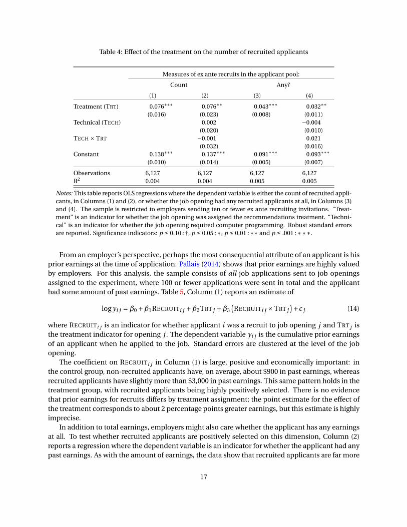
Table 4: Effect of the treatment on the number of recruited applicants

Measures of ex ante recruits in the applicant pool:

Count Any?

(1) (2) (3) (4)

Treatment (TRT) 0.076∗∗∗ 0.076∗∗ 0.043∗∗∗ 0.032∗∗

(0.016) (0.023) (0.008) (0.011)

Technical (TECH) 0.002 −0.004

(0.020) (0.010)

TECH × TRT −0.001 0.021

(0.032) (0.016)

Constant 0.138∗∗∗ 0.137∗∗∗ 0.091∗∗∗ 0.093∗∗∗

(0.010) (0.014) (0.005) (0.007)

Observations 6,127 6,127 6,127 6,127

R2 0.004 0.004 0.005 0.005

Notes: This table reports OLS regressions where the dependent variable is either the count of recruited appli-

cants, in Columns (1) and (2), or whether the job opening had any recruited applicants at all, in Columns (3)

and (4). The sample is restricted to employers sending ten or fewer ex ante recruiting invitations. “Treat-

ment” is an indicator for whether the job opening was assigned the recommendations treatment. “Techni-

cal” is an indicator for whether the job opening required computer programming. Robust standard errors

are reported. Significance indicators: p ≤ 0.10 : †, p ≤ 0.05 : ∗, p ≤ 0.01 : ∗∗ and p ≤ .001 : ∗∗∗.

From an employer’s perspective, perhaps the most consequential attribute of an applicant is his

prior earnings at the time of application. Pallais (2014) shows that prior earnings are highly valued

by employers. For this analysis, the sample consists of all job applications sent to job openings

assigned to the experiment, where 100 or fewer applications were sent in total and the applicant

had some amount of past earnings. Table 5, Column (1) reports an estimate of

log yi j =β0 +β1RECRUITi j +β2TRT j +β3

(RECRUITi j ×TRT j

)+ǫ j (14)

where RECRUITi j is an indicator for whether applicant i was a recruit to job opening j and TRT j is

the treatment indicator for opening j . The dependent variable yi j is the cumulative prior earnings

of an applicant when he applied to the job. Standard errors are clustered at the level of the job

opening.

The coefficient on RECRUITi j in Column (1) is large, positive and economically important: in

the control group, non-recruited applicants have, on average, about $900 in past earnings, whereas

recruited applicants have slightly more than $3,000 in past earnings. This same pattern holds in the

treatment group, with recruited applicants being highly positively selected. There is no evidence

that prior earnings for recruits differs by treatment assignment; the point estimate for the effect of

the treatment corresponds to about 2 percentage points greater earnings, but this estimate is highly

imprecise.

In addition to total earnings, employers might also care whether the applicant has any earnings

at all. To test whether recruited applicants are positively selected on this dimension, Column (2)

reports a regression where the dependent variable is an indicator for whether the applicant had any

past earnings. As with the amount of earnings, the data show that recruited applicants are far more

17

Table 5: Comparison of applicant characteristics by recruiting status and treatment assignment of the

applied-to job opening

Attributes of applicants to the job opening:

Log prior earnings Any prior earnings? Log profile rate Log wage bid

(1) (2) (3) (4)

Recruit (RECRUIT) 1.226∗∗∗ 0.201∗∗∗ 0.205∗ 0.322∗∗∗

(0.134) (0.014) (0.081) (0.081)

Treatment (TRT) −0.041 −0.007 −0.028 −0.039

(0.041) (0.007) (0.026) (0.031)

RECRUIT × TRT 0.061 −0.004 0.056 0.044

(0.176) (0.021) (0.102) (0.101)

Constant 6.809∗∗∗ 0.725∗∗∗ 2.042∗∗∗ 2.063∗∗∗

(0.028) (0.005) (0.019) (0.022)

Observations 63,537 87,606 54,252 54,252

R2 0.006 0.003 0.002 0.004

Notes: This table reports OLS regressions where the dependent variables are attributes of a job applicant or his

job application, at the time of application. The samples are constructed from all job applications to job openings

assigned to the experiment. The sample in Column (1) is restricted to applicants with some prior earnings at the

time of application. The Column (2) sample is the full set of applicants, regardless of past earnings. The same

sample is used for the regressions in both Column (3) and (4). The sample consists of all job applications to hourly

job openings where profile rates and wage bids were greater than one dollar but less than one hundred dollars.

“Prior earnings” are total on-platform earnings, in US dollars, by the applicant before they applied. “Profile rate” is

the hourly wage rate the worker lists on his public profile. “Wage bid” is the hourly wage bid the worker proposed

when applying for the job opening. “Recruit” indicates that the applicant was recruited by the employer in the

first hour after job-posting (i.e., an ex ante recruit). “Treatment” indicates that the job application was to a job

opening assigned to the treatment group. Standard errors are clustered at the level of the individual job opening.

Significance indicators: p ≤ 0.10 : †, p ≤ 0.05 : ∗, p ≤ 0.01 : ∗∗ and p ≤ .001 : ∗∗∗.

18

likely to have past on-platform earnings (90% versus a little more than 70%). Further, the same

pattern holds in both the treatment and control groups, with no significant differences by group.

Another measure employers care about is a worker’s past wage rate. When a worker applies to

an hourly job opening, his wage bid and profile rates are recorded. Columns (3) and (4) report re-

gressions where the dependent variables are the log profile rate and log wage bid of the applicant,

respectively. The samples for both estimates are restricted to applications sent to hourly job open-

ings where both the profile rate and hourly charge rate were above one dollar but less than one hun-

dred dollars. As with earnings, the large, positive coefficient on the RECRUIT indicator shows that

recruits are positively selected: profile rates are about 25% higher (from Column (3)) and wage bids

are about 40% higher (from Column (4)). The coefficient on the interaction term is positive and on

the order of about 5 percentage points, though the estimates are imprecise and far from significant.

If not a statistical artifact, the positive interaction term suggests that treatment-induced recruits

were somewhat more expensive. Despite this possibility, at least within the limits of available sta-

tistical power, experimentally induced recruited applicants are similar to those in the control group

in terms of past on-platform earnings (both amount and existence), wages bids and profile rates.

5.5 Employer screening, measured at the individual applicant level

Before employers make a hire, they evaluate, or “screen” their applicant pools. Not all applicants are

screened; employers make choices about which applicants to screen on the basis of their observ-

able characteristics. It is beyond the scope of this paper to model the employer’s screening decision

problem fully, but it is useful to see whether employers show any bias in their screening with re-

spect to the treatment and the recruiting status of applicants. Table 6 shows that: (1) employers are

substantially more likely to screen recruited applicants, (2) there is no evidence of screening “crowd

out” of non-recruited applicants in the treatment (despite the treatment raising recruited applicant

counts) and that (3) there is no strong evidence that screening probability differed for recruits by

the treatment assignment of the applied-to job opening.

Table 6, Column (1) reports an estimate of the regression

SCREENEDi j =β0 +β1(TRT j ×RECRUIT j )+β2TRT j +β3RECRUIT j +ǫ j , (15)

where SCREENEDi j is an indicator for whether the employer screened applicant i to job opening j .

The sample consists of all job applications and standard errors are clustered at the level of the job

opening. From the intercept, it is apparent that the baseline screening rate is high but not nearly

100%—about 65% of organic applicants are screened. However, recruited applicants are at an ad-

vantage: their screening rate in the control group is slightly more than 9 percentage points higher.

There is no strong evidence that screening rates depend on the treatment assignment of the associ-

ated job opening for either recruits or organic applicants.

To test for differential screening by the nature of work, I estimate the Column (1) regression for

the two types of jobs separately. Column (2) reports the same applicant-level screening regression

as in Column (1) but for applications to technical job openings; Column (3) reports results for appli-

cants to non-technical job openings. While in both samples recruits are more likely to be screened,

the advantage is smaller for technical job openings. However, the Column (2) intercept shows that

the baseline probability of screening for technical job openings is higher by about 10 percentage

points compared to non-technical job openings, leaving less “room” for a large difference between

19

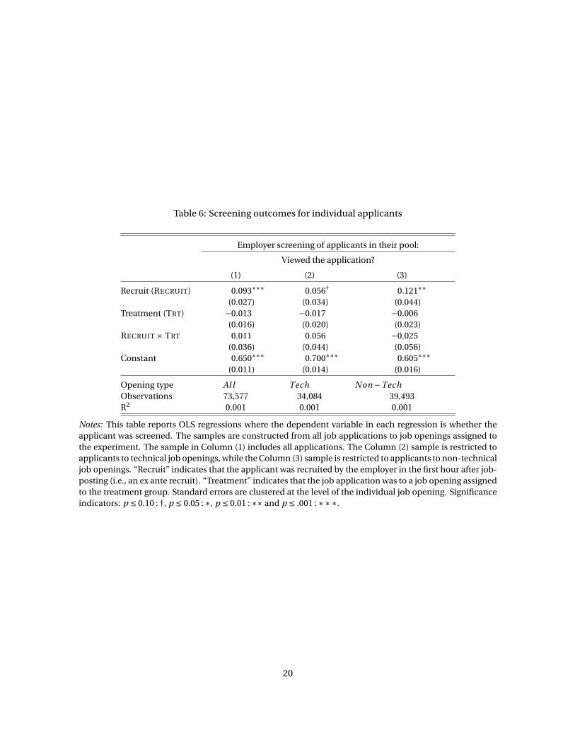
Table 6: Screening outcomes for individual applicants

Employer screening of applicants in their pool:

Viewed the application?

(1) (2) (3)

Recruit (RECRUIT) 0.093∗∗∗ 0.056† 0.121∗∗

(0.027) (0.034) (0.044)

Treatment (TRT) −0.013 −0.017 −0.006

(0.016) (0.020) (0.023)

RECRUIT × TRT 0.011 0.056 −0.025

(0.036) (0.044) (0.056)

Constant 0.650∗∗∗ 0.700∗∗∗ 0.605∗∗∗

(0.011) (0.014) (0.016)

Opening type All Tech Non −Tech

Observations 73,577 34,084 39,493

R2 0.001 0.001 0.001

Notes: This table reports OLS regressions where the dependent variable in each regression is whether the

applicant was screened. The samples are constructed from all job applications to job openings assigned to

the experiment. The sample in Column (1) includes all applications. The Column (2) sample is restricted to

applicants to technical job openings, while the Column (3) sample is restricted to applicants to non-technical

job openings. “Recruit” indicates that the applicant was recruited by the employer in the first hour after job-

posting (i.e., an ex ante recruit). “Treatment” indicates that the job application was to a job opening assigned

to the treatment group. Standard errors are clustered at the level of the individual job opening. Significance

indicators: p ≤ 0.10 : †, p ≤ 0.05 : ∗, p ≤ 0.01 : ∗∗ and p ≤ .001 : ∗∗∗.

20

technical and non-technical job openings. As in Column (1), there is no strong evidence that screen-

ing rates depend on treatment assignment, though the point estimate on the recruit indicator and

treatment indicator interaction in Column (2) is more than 5 percentage points. This would be an

economically important effect, but it is not significant. If it is not a statistical artifact, it suggests

that treatment-induced recruits for technical job openings were more likely to be screened.

5.6 Employer hiring

The primary goal of offering algorithmic recommendations was to increase hiring. Table 7 shows

that recommendations were effective at increasing hires, but only unambiguously so for technical

job openings. The differential treatment effectiveness does “show up” in the overall analysis in that

treated job openings were more likely to surpass $500 in total wages paid, which is close to the me-

dian spend per job. This finding is consistent with the treatment increasing formation of relatively

technical job matches, which tend to have higher wage bills. Hypotheses for why treatment effects

differed by the type of work will be explored in subsequent sections, but first I simply present the

results. Among technical job openings, I find no evidence of crowd-out of organic applicants, but I

show that given the size of the point estimates of the treatment, it would be unlikely to find strong

crowd-out.

Column (1), Table 7 reports an estimate of

EMPHIRED j =β0 +β1TRT j +ǫ (16)

where EMPHIRED j is an indicator for whether some amount of money was spent by the employer

on a worker hired for job opening j . The coefficient on the treatment indicator is positive, with a

magnitude of nearly 2 percentage points, but this estimate is not conventionally significant. Col-

umn (2) reports the same regression as Column (1), but with the sample restricted to technical job

openings. Among technical job openings, the treatment increased the probability that a hire was

made by more than 4 percentage points, from a base of only 22%. This sub-group effect is easily still

significant under the conservative Bonferroni correction for multiple hypotheses testing.

The increase in the fill rate among technical job openings shown by Column (2)—a 4.3 percent-

age point increase—is a large effect. Too large, in fact, to be credibly explained solely by the direct

channel of increased ex ante recruiting. Recall that the treatment increased recruiting by 7.3 per-

centage points among technical job openings. Technical job openings in the control group had a

baseline recruiting rate of 15% and a fill-from-recruits rate of 3.8%. If one assumes that the marginal

increase in recruits from the treatment “converted” to hires at the same rate in the treatment as in

the control, the treatment effect in Column (2) should be (1/4)0.07 ≈ 1.8%. This is close to the

treatment effect of 2 percentage points found in the Column (2) regression, where the dependent

variable is whether the employer hired an ex ante recruit.

The “extra” increase in hiring find in Column (2) comes from the firm hiring organic applicants:

Column (3) reports a regression where the dependent variable is the firm hiring an organic appli-

cant, and as expected, the coefficient on the treatment indicator is positive and has the right mag-

nitude to explain the overall increase in hiring. Although the coefficient on the treatment indicator

in Column (4) is not conventionally significant, recall from the employer recruiting model that the

treatment effect should be negative because recruits should crowd out non-recruited applicants.

The lack of crowd-out—and perhaps even complementarity—may seem surprising, but not

if one considers the overall low fill rate. Crowd-out would occur among employers who would

21

Table 7: Effects of the recommendations treatment on hiring

Dependent variable:

Hire Made Hired Early Recruit Hired Organic

All Technical Technical Technical

(1) (2) (3) (4)

Treatment 0.019 0.043∗∗∗ 0.020∗∗∗ 0.022

(0.011) (0.015) (0.007) (0.015)

Constant 0.276∗∗∗ 0.216∗∗∗ 0.032∗∗∗ 0.212∗∗∗

(0.008) (0.010) (0.004) (0.010)

Observations 6,209 3,136 3,136 3,136

R2 0.0004 0.003 0.002 0.001

Notes: This table reports several regressions where the outcome variables are measures of employer hiring, using data

from the recommendations experiment. Each regression was estimated using OLS, and robust standard errors are re-

ported. The key independent variable across across regressions is the indicator for whether the vacancy was assigned to

the treatment group. The dependent variable in each of these regressions is whether or not the employer hired a worker

of a particular type. In Columns (1) and (2) the indicator is for hiring anyone at all. In Column (1) the sample is all va-

cancies, while in Column (2) the sample consists of only technical vacancies. In Column (3) the outcome is whether the

employer hired a recruited applicant, while in Column (4) the outcome is whether the employer hired an organic appli-

cant. In both Columns (3) and (4) the sample is restricted to technical vacancies. Significance indicators: p ≤ 0.10 : †,

p ≤ 0.05 : ∗, p ≤ 0.01 : ∗∗ and p ≤ .001 : ∗∗∗.

have hired an organic applicant when in the control but would instead hire a recruited applicant

when in the treatment. Column (3) shows that only 20% of employers in the control group hired

an organic applicant, 3% hired a recruit and the rest did not hire anyone. If the approximately 7

percentage point increase in recruiting caused by the treatment was uniform across all of these

segments, then one would see a (0.07)(0.20) ≈ 1.4% increase in recruiting among organic-hiring

control employers if they had counter-factually received the treatment. Under the assumption

that the conversion rate of recruits into hires is the same value, i.e., ∼ (1/4) and that every one of

these hired recruits displaced an organic applicant, the reduction in organic hiring would only be

(1/4)(0.014) ≈ −0.0035, which is a very small effect. Of course, if the fill rate were higher—or if the

treatment was heterogeneous—then crowd-out could become substantial.

5.7 Hiring at the applicant level

In addition to measuring hiring at the level of the job opening, it is useful to consider hiring at the

level of the individual applicant. The applicant-level view allows me to test whether employers show

a preference for recruited applicants and whether their preferences depended on the treatment as-

signment and nature of work. Table 8 shows that recruited applicants are far more likely to be hired

in general for both technical and non-technical categories of work. This preference partially ex-

plains why the treatment can have such a strong effect on hiring despite the number of induced

applicants from the treatment being small relative to the size of the applicant pool. As one would

expect given that the treatment increased the number of recruited applicants but not the fraction

of employers hiring recruits for that category, there is some evidence that treatment-induced ap-

plicants in non-technical categories of work have a lower hire rate than their control counterparts.

22

A potential reason for this difference is explored in the next section in which I compare recruited

applicants across experimental groups and categories of work on the basis of their observable char-

acteristics.

Table 8: Hiring outcomes by treatment assignment job opening type and recruit status

Dependent variable:

Applicant Hired?

(1) (2) (3)

Recruit (RECRUIT) 0.103∗∗∗ 0.083∗∗∗ 0.129∗∗∗

(0.015) (0.018) (0.024)

Treatment (TRT) 0.001 0.003∗ −0.001

(0.001) (0.001) (0.001)

RECRUIT×TRT −0.010 0.022 −0.047

(0.019) (0.026) (0.028)

Constant 0.015∗∗∗ 0.015∗∗∗ 0.016∗∗∗

(0.001) (0.001) (0.001)

SEs clustered at job opening? Y Y Y

Include Tech? Y Y N

Include Non-Tech? Y N Y

Observations 73,577 34,084 39,493

R2 0.011 0.011 0.011

Notes: This table reports OLS regressions where the dependent variable in each regression is whether the

applicant was hired. The samples are constructed from all job applications to job openings assigned to the

experiment. The sample in Column (1) includes all applications. The Column (2) sample is restricted to

applicants to technical job openings, while the Column (3) sample is restricted to applicants to non-technical

job openings. “Recruit” indicates that the applicant was recruited by the employer in the first hour after job-

posting (i.e., an ex ante recruit). “Treatment” indicates that the job application was to a job opening assigned

to the treatment group. Standard errors are clustered at the level of the individual job opening. Significance

indicators: p ≤ 0.10 : †, p ≤ 0.05 : ∗, p ≤ 0.01 : ∗∗ and p ≤ .001 : ∗∗∗.

Column (1), Table 8 reports an estimate of

HIREDi j =β0 +β1RECRUITi j +β2TRT j +β3

(RECRUITi j ×TRT j

)+ǫ j (17)

where the sample is all applicants to a job opening and the HIREDi j is an indicator for whether

worker i was hired for job opening j . Standard errors are clustered at the level of the individual job

opening. The constant terms from Column (1) shows that the baseline hire rate for organic appli-

cants in the control is about 1.5%, but for recruits, this goes up by slightly more than 10 percentage

points. There is no evidence that these hire rates differ substantially by treatment assignment.

In Column (2), the sample is restricted to job applicants to technical job openings. The hire rate

for recruits in the control is about 2 percentage points lower than the hire rate in the control from

Column (1), but a formal hypothesis test would fail to reject a null of no difference in the point es-

timates. Where there is a difference is in the hire rate of organic applicants in the treatment—the

coefficient on the treatment indicator is about 3/10ths of a percentage point. Given the finding of a

higher rate of organic hires in the treatment group for technical categories, this result is, in a sense,

mechanically expected. However, the greater statistical precision offered by the job applicant view

23

of Table 8 and the resultant stronger finding raises the question of whether the increased hiring of

organic applicants in the treatment, for technical job openings, is not simply a statistical artifact.

One interesting possibility is that the existence of recruited applicants increased employer screen-

ing on either the extensive or intensive margins, which in turn “spilled over” onto non-recruits,

though this is highly speculative.9

To investigate the technical/non-technical distinction further, in Column (3) the sample is re-

stricted to non-technical job openings. As in the other regressions, there is a large positive coef-

ficient on the recruit indicator, showing a strong preference among control employers for hiring

recruited applicants for non-technical job openings. The coefficient is larger than in Column (1),

but the standard errors are large enough that a formal hypothesis test would reject a difference in

hiring preference for recruits across samples. Unlike technical job openings, there is no evidence

that non-technical organic applicants benefited from the treatment—the coefficient on the treat-

ment indicator is very close to zero and precisely estimated. The coefficient on the recruit indicator

and treatment indicator interaction term is large in magnitude and negative, as expected given that

the treatment increased recruiting but not hiring. The possibility that treatment-induced recruits

for non-technical job openings systematically differed is the focus of the next section.

5.8 Comparison of ex ante recruits by job opening type and associated treatment assign-

ment

One potential explanation for why the treatment was only effective for technical job openings was

that the algorithm delivered relatively poorer recommendations for non-technical job openings. Ta-

ble 9 compares recruits across experimental groups and categories of work to look for differences.

Within the limits of the statistical power available, there are no statistically significant differences

in ex ante recruits across experimental groups, conditioned on the job type. However, there is some

evidence that the recruits induced by the treatment were relatively more experienced and thus more

expensive. If experimentally induced non-technical recruits were in fact relatively more expensive,

it could explain why they have a lower hire rate. A difference in price could have a magnified effect

in non-technical categories, as Horton and Johari (2015) show that employers in non-technical cat-

egories of work are far more price sensitive than those hiring in technical categories of work. While

higher relative cost is an attractive explanation, the general imprecision of these estimates make it

difficult to reach strong conclusions.

Column (1), Table 9 reports an estimate

log yi j =β0 +β1TRTi j +β2TECHNICAL j +β3

(TECHNICALi j ×TRT j

)+ǫ j (18)

where the sample is restricted to ex ante recruits and yi j is the past cumulative earnings of applicant

i to job opening j . Standard errors are clustered at the level of the job opening. As expected, the

coefficient on the technical indicator is positive and very large: recruits to technical job openings

have nearly 70% higher earnings. The coefficient on the treatment indicator is small—implying little

more than a 1 percentage point increase in earnings for recruits to non-technical job openings—but

the estimate is highly imprecise. The technical and treatment interaction is large as a point estimate,

9In a re-analysis of several well-known correspondence studies, Phillips (2015) argues that designs that sent multiple applica-

tions to the same employer induced exogenous variation in applicant pool quality which in turn generated search externalities.

24

Table 9: Comparison of recruited applicant characteristics, by treatment assignment

Dependent variable:

Log prior earnings Any prior earnings? Log profile Rate Log wage Bid

(1) (2) (3) (4)

Technical (TECH) 0.694∗∗ 0.012 0.667∗∗∗ 0.690∗∗∗

(0.256) (0.028) (0.135) (0.133)

Treatment (TRT) 0.049 0.004 0.127 0.104

(0.227) (0.029) (0.124) (0.124)

TECH×TRT 0.168 −0.032 −0.067 −0.066

(0.323) (0.041) (0.176) (0.171)

Constant 7.643∗∗∗ 0.920∗∗∗ 1.845∗∗∗ 1.970∗∗∗

(0.174) (0.021) (0.094) (0.096)

SE’s clustered at job opening? Y Y Y Y

Observations 1,340 1,460 961 961

R2 0.035 0.001 0.141 0.153

Notes: This table reports OLS regressions where the dependent variables are attributes of an ex ante recruited job

applicant or his job application, at the time of application. The samples are constructed from all job applications

by ex ante recruits to job openings assigned to the experiment. The sample in Column (1) is restricted to applicants

with some prior earnings at the time of application. The Column (2) sample is the full set of applicants, regardless

of past earnings. The sample used for both Column (3) and (4) is the same. It consists of all job applications

to hourly job openings where profile rates and wage bids were greater than one dollar but less than one hundred

dollars. “Prior earnings” are total on-platform earnings, in US dollars, by the applicant before they applied. “Profile

rate” is the hourly wage rate the worker lists on his public profile. “Wage bid” is the hourly wage bid the worker

proposed when applying for the job opening. “Recruit” indicates that the applicant was recruited by the employer

in the first hour after job-posting (i.e. an ex ante recruit). “Treatment” indicates that the job application was to a job

opening assigned to the treatment group. Standard errors are clustered at the level of the individual job opening.

Significance indicators: p ≤ 0.10 : †, p ≤ 0.05 : ∗, p ≤ 0.01 : ∗∗ and p ≤ .001 : ∗∗∗.

25

implying a 17 percentage point increase in the treatment, but again, the estimate is highly imprecise

and far from conventionally significant.

In Column (2) the dependent variable is an indicator for any prior earnings. As compared to

prior earnings, precision is better and the differences by group and job type are small—though given

that over 90% of recruits have some prior experience, there is little room for large differences. On

profile rates (in Column (3)) and wage bids (Column (4)), it is apparent that technical recruits have

far higher profile rates and submit higher bids. Note that for these regressions the sample is limited

to hourly job openings.

Also mirroring the pattern from Column (1), the standard errors are large enough to contain

economically important effects comfortably. For example, the coefficient on the treatment indica-

tor implies that wage bids and profile rates were about 10% higher for recruits to non-technical job

openings in the treatment than in the control. These results are not conventionally significant—far

from it in fact—but if the point estimates are correct, it would imply that the algorithmic recom-

mendations were inducing relatively more expensive applicants for non-technical openings. The

coefficient on the technical and treatment interaction term is negative, implying that experimen-

tally induced technical recruits were relatively cheaper—but again, this effect is far from significant.

5.9 Treatment effects on hiring, conditioned by predicted organic applicant count

In the model presented in Section 4.1, a reduction in recruiting costs increases the number of re-

cruits for all employers, but the effects on fill rates are larger for employers with smaller expected

applicant pools. This aspect of the model potentially provides a parsimonious explanation for the

technical/non-technical difference in treatment effectiveness. Because employers with technical

job openings have smaller applicant pools, they value the pool-expanding effects of the treatment

more than employers with non-technical job openings.

It is tempting to test this hypothesis by conditioning the treatment indicator on the realized

count of organic applicants and test for heterogeneous effects. However, using the realized organic

application count as a regressor is problematic. First, idiosyncratic job opening attributes might af-

fect both the count of applicants received and the baseline probability of a hire being made. Second,

the count of organic applications could be affected by the treatment—if, for example, the employer

makes a quick hire because she has access to the treatment. This possibility makes the organic

applicant count an inappropriate right-hand-side variable.

Rather than use the realized application count, I instead use the predicted organic application

count, with predictions derived from a machine learning model fit only with pre-randomization job

opening attributes—see Appendix C for details on the predictive model. I estimate the effects of the

treatment on hiring, conditional upon predicted organic application counts. Table 10 shows that

the returns from the treatment depend strongly upon the predicted organic applicant count, with

effectiveness decreasing in the predicted applicant pool size. This dependency offers a parsimo-

nious explanation for the difference in treatment effects on hiring for technical and non-technical

job openings.

Table 10, Column (1) reports an estimate of

HIRED j =β0 +β1TRT j +β2�log A j +β3

(TRT j × �log A j

)+ǫ j , (19)

where HIRED j is an indicator for whether a hire was made against that job opening and �log A j is

26

Table 10: Effects of the recommendations treatment, conditioned upon predicted organic applicant

counts

Dependent variable:

Hire made?

(1) (2) (3)

Treatment (TRT) 0.081∗ 0.104† 0.044

(0.040) (0.059) (0.054)

Predicted log num organic apps ( �log A) 0.053∗∗∗ 0.011 0.072∗∗∗

(0.012) (0.019) (0.016)

TRT × �log A −0.029 −0.029 −0.024

(0.018) (0.027) (0.024)

Constant 0.161∗∗∗ 0.193∗∗∗ 0.180∗∗∗

(0.028) (0.041) (0.037)

Include Tech? Y Y N

Include Non-Tech? Y N Y

Observations 6,209 3,136 3,073

R2 0.004 0.003 0.009

Notes: This table reports OLS regressions where the dependent variable is whether the employer

made a hire. In Column (1), the entire experimental sample is used, while in Columns (2) and (3),

the sample consists of all technical and non-technical job openings, respectively. In each regres-

sion, the treatment indicator is interacted with the prediction of how many organic applicants

the job opening would receive. See Appendix C for details on the predictive model. Significance

indicators: p ≤ 0.10 : †, p ≤ 0.05 : ∗, p ≤ 0.01 : ∗∗ and p ≤ .001 : ∗∗∗.

27

the log predicted count of organic applicants for opening j . The sample for Column (1) is all job

openings assigned to the experiment. The coefficient on the treatment indicator is positive and

large: when the predicted organic applicant count is one (as log(1) = 0), the model implies the

treatment causes an 8 percentage point increase in hiring. Recall that estimated treatment effect

on hiring for the full sample was about 2 percentage points (and not conventionally significant).

This is not a wildly out-of-sample extrapolation, as a substantial fraction of job openings receive

just a small number of organic applicants. The coefficient on the treatment and predicted appli-

cant count interaction term is negative, implying that as the count of organic applicants increases,

the treatment is less effective at increasing hiring. In effect, the treatment and organic applicants

are substitutes. If one takes the linear model seriously, the treatment no longer has a positive ef-

fect at exp(0.80/(0.054−0.028)) ≈ 22 applicants. However, there are good reasons to not take it too

seriously—in Columns (2) and (3) I estimate the model separately for technical and non-technical

jobs and find important qualitative differences by category of work.

Column (2) is the same regression as Column (1), but with the sample restricted to technical job

openings. Compared to the Column (2) regression, both the coefficient on the treatment indicator

and the interaction term are similar in magnitude. However, the returns to predicted organic appli-

cants are only a fifth of what they were in the full estimate from Column (1). Of course, the count

of predicted organic applicants is not as good as randomly assigned, and as such, the coefficient

cannot be interpreted causally. However, much of the variation in the predicted applicant count is

likely due to supply factors—the sub-category of work is by far the most important component of

the predictive model. To the extent that there is exogenous variation in organic applicant counts, the

evidence suggests that technical job openings get little value from the marginal organic applicant.

This is consistent with Horton and Johari (2015) in that employers with technical job categories are

much less price sensitive and thus would have a relative preference for the higher quality but higher

wage applicants that come through the employer recruiting channel.

Column (3) is the same regression as Column (1), but with the sample restricted to non-technical

job openings. The coefficient on the treatment indicator is positive—recall that it was negative with-

out conditioning on the predicted organic applicant count. However, it is substantially smaller than

the effect estimates from Column (2), which was the technical-only regression. The interaction term

is negative and similar in magnitude to the other estimates, suggesting that as with technical jobs,

organic applicants and recruits are substitutes. The big qualitative difference in Column (3) versus

the other regressions is in the returns to more organic applicants: as the organic application count

increases, hiring goes up substantially, with an effect about six times larger than the estimate from

the technical job openings.

6 Discussion

The main results of the experiment are clear: (1) employers act upon recommendations, with the

effect mainly being on the extensive margin; (2) recommendations deliver additional applicants

similar to the kinds of workers that employers recruit on their own; (3) the recommendations were

effective at increasing hiring in technical job openings, without any detectable crowd-out of non-

recruited organic applicants.

Explaining (1) and (2) is fairly straightforward: the treatment lowered the cost of recruiting, and

more employers decided to recruit. The comparison of ex ante recruited applicants and organic

28

applicants shows that recruits—in both the treatment and control groups—are highly positively

selected. By delivering more applicants that “look like” the kinds of applicants employers have a

strong preference for hiring, hiring increased at least for some types of openings. Before discussing

the technical/non-technical treatment effect heterogeneity, it is useful to consider explanations for

treatment efficacy and compare them to other facts uncovered by the applicant-level analyses.

There is no evidence that the main effect of the experiment was simply to alert employers to

the possibility of recruiting, as the treatment did not increase “late” recruiting. The treatment-

induced recruited workers who applied were similar on observables to the kinds of workers employ-

ers tend to recruit, and employers screened and hired these recruits at similar rates—undercutting

the notion that employers regarded the treatment-induced recruits as better or worse than their

observables would suggest. Furthermore, there is some “downstream” evidence of comparability

of experimentally-induced recruits to control groups: if the treatment caused employers to believe

that their pools were more productive than the control, even conditioning on observables, then

they would, on average, be relatively disappointed by realized performance, and yet there is no

evidence of this—treatment and control matches look very similar with respect to all measures of

match quality. (Match quality analysis is in Appendix B).

The largest puzzle in the experimental results is why the treatment only increased hiring for

technical job openings. There is no strong evidence that the recommendations were any worse for

non-technical job openings: recruits were similar on observables, and “uptake” by employers and

workers was the same by type of work and by experimental group. If there is a difference, it is that

non-technical treatment recruits tended to be slightly more expensive than their control counter-

parts. The explanation most consistent with all the facts is that technical job openings differed from

non-technical job openings in two important ways. First, technical job openings generally get fewer

applicants and value the marginal applicant more. Second, employers with technical job openings

are less price sensitive and value higher quality applicants relatively more than employers with non-

technical job openings. As the algorithmic recommendations deliver more applicants—particularly

higher quality and higher cost applicants—the treatment is more useful in technical categories of

work.

7 Conclusion

In this paper, I demonstrate that algorithmic recommendations are both acted upon by employers

and also effective at raising hiring, at least for some kinds of job openings where more applicants

of high quality are valued. While the algorithm is a “black box,” it delivers recommendations obser-

vationally identical to the kinds of workers employers recruit in the absence of these recommenda-

tions, at least within the limits of available measurements and statistical power. As such, it makes

sense to think of algorithmic recommendations as substituting for costly employer effort.

A novel feature of this experiment was that it was focused on helping the demand side of the

labor market; most other active labor market policies have focused on the supply side. Perhaps the

encouraging results from this study and its demand-side focus are a coincidence, but an intriguing

possibility is that serving firms is more fruitful than serving workers. There is a superficial symmetry

between job openings and workers; job openings can be readily created and destroyed by employ-

ers at will, and while workers do enter and exit the labor market, it seems likely that the employer

decision to create and fill an opening is more elastic with respect to assistance than an individual

29

worker. Turning to the conventional market analogue of this experiment, for-profit recruiting firms

offer their services primarily to companies rather than individuals.

In terms of generalizability, these results come from a context where search frictions are already

very low, suggesting that bigger gains are possible in traditional, more friction-prone markets. As

more of the labor market becomes computer-mediated, the possibilities for platform-based inter-

ventions grow in scope and power. Platforms invariably collect enormous amounts of data on mar-

ket behaviors and outcomes; they also have nearly full control over what information market partic-

ipants can see, and when. This possibility could have enormous equity and efficiency consequences

for labor markets, and more studies on how to use this power constructively are needed.

30

References

Adomavicius, Gediminas and Alexander Tuzhilin, “Toward the next generation of recommender systems: A sur-

vey of the state-of-the-art and possible extensions,” IEEE Transactions on Knowledge and Data Engineering,

2005, 17 (6), 734–749.

Agrawal, Ajay K., John Horton, Nico Lacetera, and Elizabeth Lyons, “Digitization and the contract labor market:

A research agenda,” in “Economics of Digitization,” University of Chicago Press, 2013.

, Nicola Lacetera, and Elizabeth Lyons, “Does information help or hinder job applicants from less developed

countries in online markets?,” January 2013, (NBER Working Paper 18720).

Autor, David H and David Scarborough, “Does job testing harm minority workers? Evidence from retail establish-

ments,” The Quarterly Journal of Economics, 2008, pp. 219–277.

Barron, John M. and John Bishop, “Extensive search, intensive search, and hiring costs: New evidence on em-

ployer hiring activity,” Economic Inquiry, 1985, 23 (3), 363–382.

, Dan A. Black, and Mark A. Loewenstein, “Job matching and on-the-job training,” Journal of Labor Economics,

January 1989, 7 (1), 1–19.

Burdett, Kenneth and Elizabeth J. Cunningham, “Toward a theory of vacancies,” Journal of Labor Economics, July

1998, 16 (3), 445–78.

Card, David, Jochen Kluve, and Andrea Weber, “Active labour market policy evaluations: A meta-analysis,” The

Economic Journal, 2010, 120 (548), F452–F477.

Crépon, Bruno, Esther Duflo, Marc Gurgand, Roland Rathelot, and Philippe Zamora, “Do labor market poli-

cies have displacement effects? Evidence from a clustered randomized experiment,” The Quarterly Journal of

Economics, 2013, 128 (2), 531–580.

Friedman, Jerome, Trevor Hastie, and Robert Tibshirani, “glmnet: Lasso and elastic-net regularized generalized

linear models,” R package version, 2009, 1.

Gautier, Pieter, Paul Muller, Bas van der Klaauw, Michael Rosholm, and Michael Svarer, “Estimating equilibrium

effects of job search assistance,” IZA Discussion Papers 6748, Institute for the Study of Labor (IZA) July 2012.

Gibbons, Robert and Lawrence F Katz, “Layoffs and lemons,” Journal of Labor Economics, 1991, pp. 351–380.

Hoffman, Mitch, Lisa B Kahn, and Danielle Li, “Discretion in hiring,” Working Paper, 2015.

Horton, John, “Price floors and preferences: Evidence from a minimum wage experiment,” Working Paper, 2015.

and Ramesh Johari, “At what quality and what price? Eliciting buyer preferences as a market design problem,”

Working Paper, 2015.

Kluve, Jochen, “The effectiveness of european active labor market programs,” Labour Economics, 2010, 17 (6),

904–918.

Kuhn, Peter and Hani Mansour, “Is Internet job search still ineffective?,” The Economic Journal, 2014, 124 (581),

1213–1233.

and Mikal Skuterud, “Internet job search and unemployment durations,” The American Economic Review, 2004,

94 (1), 218–232.

Oyer, Paul and Scott Schaefer, “Personnel economics: Hiring and incentives,” May 2010, (15977).

31

Pallais, Amanda, “Inefficient hiring in entry-level labor markets,” American Economic Review, March 2014,

(18917).

Pellizzari, Michele, “Employers’ search and the efficiency of matching,” British Journal of Industrial Relations,

2011, 49 (1), 25–53.

Phillips, David C., “Search externalities and bias in correspondence experiments: Evidence from randomly as-

signed applicant pools,” Working Paper, 2015.

Resnick, Paul and Hal R. Varian, “Recommender systems,” Communications of the ACM, 1997, 40 (3), 56–58.

Stanton, Christopher and Catherine Thomas, “Landing the first job: The value of intermediaries in online hiring,”

Available at SSRN 1862109, 2012.

Tibshirani, Robert, “Regression shrinkage and selection via the lasso,” Journal of the Royal Statistical Society. Series

B (Methodological), 1996, pp. 267–288.

van Ours, Jan and Geert Ridder, “Vacancies and the recruitment of new employees,” Journal of Labor Economics,

1992, 10 (2), 138–155.

Varian, Hal R., “Computer mediated transactions,” American Economic Review, 2010, 100 (2), 1–10.

32

A Internal validity

A.1 Randomization

Job openings were randomly assigned to the treatment or control group after being posted to the

marketplace. As such, pre-assignment covariates describing vacancy should be balanced across the

groups; the count of observations across groups should also be consistent with a random process.

In Table A1, I confirm this is the case. In the top panel, I report the count of observations and the p-

value for a χ2 test. I cannot reject the null hypothesis of an identical assignment probability across

the groups. In the lower panel, I report the fraction of vacancies of different “types” (by category of

work) by experimental group. I also report two non-category covariates—an indicator for whether

the length of job description exceeded the median and whether the employer required that appli-

cants have prior on-platform work experience. For each covariate, I report the mean and standard

error for each group; I also report the difference in means, the standard error for that difference and

the p-value for a two-sided t-test. I find good balance across the collection of covariates chosen,

with none of the t-test p-values being conventionally significant.

A.2 SUTVA

One concern with a field experiment is that the treatment cells interact with each other in some

way, violating the stable unit treatment value assumption (SUTVA) required for causal inference.

Any sufficiently large experiment conducted in a marketplace risks SUTVA problems. In this ex-

perimental setting, “deep” SUTVA concerns (say, moving the market or changing the incentive to

entry or exit) are probably unwarranted. First, this experiment was conducted a year after Pallais

(2014), who did find evidence of market-moving effects, and the market was at least twice as large

when this experiment was run. Further, unlike her experiment, vacancies associated with all types

of work were eligible. And because only new employers were eligible for the experiment and only

some of these were allocated, only about 6% of the vacancies posted during the experimental period

were actually assigned to the experiment (and only 1/2 of those were in the active treatment).

B Auxiliary Analyses

B.1 Job opening applicant counts

Although the treatment increased the number of recruited applicants, did it increase the size of

the applicant pool in total? While the data are consistent with this hypothesis—treated employers

had larger applicant pools on average—this difference in mean counts is very imprecisely estimated

and far from conventionally significant. Table A2 shows that even with transformations designed to

reduce the standard error, treatment estimates are quite imprecise.

In Column (1), the coefficient on the treatment indicator is positive, but imprecisely estimated.

The high variance in the per-opening number of applicants makes it difficult to detect any treat-

ment effects. In Column (2) I winsorize the per-opening number of applicants with a ceiling of 50.

This shrinks the standard error, but it also reduces the effect size, implying that some treatment

openings had very high application counts.

33

Table A1: Pre-treatment covariate means by experimental group

Treatment

mean:

XT RT

Control

mean:

XC T L

Difference in

means:

XT RT − XC T L

p-value

Observation Counts

3,027 3,182 1.7

Type of work

Technical (1 if yes, 0 otherwise) 0.500 (0.009) 0.510 (0.009) -0.011 (0.013) 0.392

Non-Technical 0.500 (0.009) 0.490 (0.009) 0.011 (0.013) 0.392

Type of work—(more detailed)

Admin 0.081 (0.005) 0.081 (0.005) -0.000 (0.007) 0.947

Writing 0.126 (0.006) 0.122 (0.006) 0.004 (0.008) 0.611

Web 0.375 (0.009) 0.389 (0.009) -0.014 (0.012) 0.243

Design 0.114 (0.006) 0.115 (0.006) -0.001 (0.008) 0.897

Software 0.125 (0.006) 0.121 (0.006) 0.004 (0.008) 0.670

Vacancy attributes

Job description length > median 0.562 (0.009) 0.572 (0.009) -0.010 (0.013) 0.441

Required prior oDesk experience 0.120 (0.006) 0.109 (0.006) 0.011 (0.008) 0.179

Notes: This table reports data from a recommendation experiment conducted on the oDesk platform. In the experiment, the

treated group of employers received algorithmically-generated recommendations of candidates for their vacancies while the

control group did not. The unit of randomization was the posted vacancy. The top panel, labeled “Observation Counts,” is the

number of vacancies per experimental group. The “Observation Counts” panel p-value is for a two-sided test of equal group

assignment probabilities; the the p-value was calculated by simulation, using the fact that 13,259 potential employers were

allocated, but only 5,953 generated usable vacancies for assignment. In the lower panels, for each variable, we report the mean

and standard error for various pre-treatment covariates, as well standard error for the cross-group differences. The p-value

column is for a two-sided t-test against the null hypothesis of no difference in means across the treatment and control groups.

In the middle panels (“Type of Work” and “Type of work—(mode detailed)”), the covariantes are indicators for whether the

vacancy was for a particular type of work. In the bottom panel, the two covariates are (1) an indicator for whether the employer

required that applicants have prior oDesk experience and (2) whether the count of text characters in the job description was

greater than the median count for the pooled sample of all job descriptions in the experiment. Significance indicators: p ≤

0.10 : †, p ≤ 0.05 : ∗, p ≤ 0.01 : ∗∗ and p ≤ .001 : ∗∗∗.

34

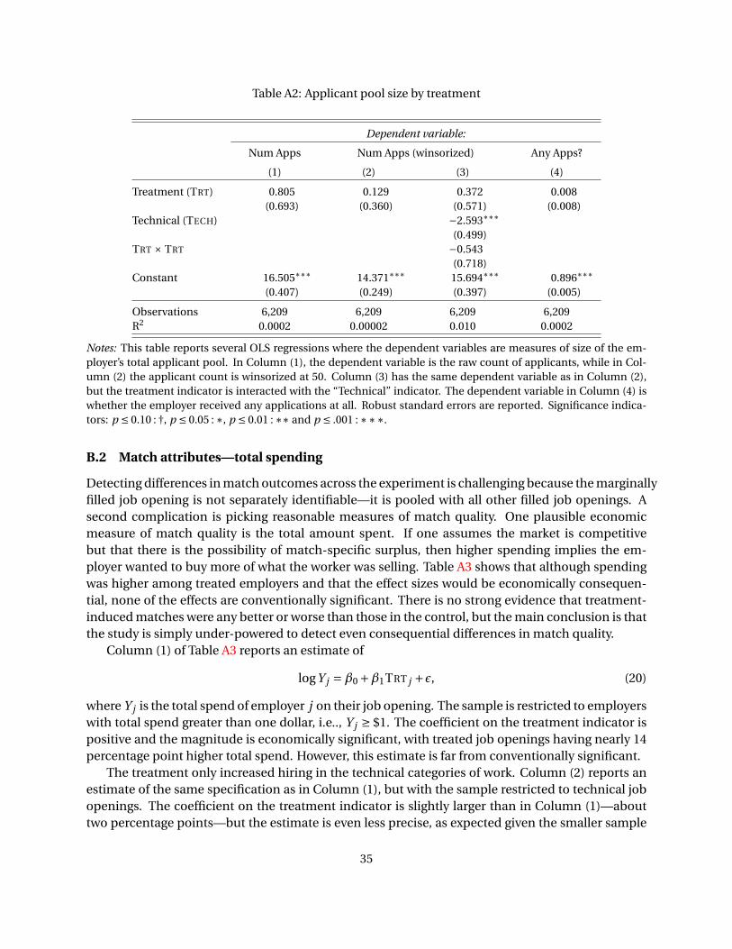
Table A2: Applicant pool size by treatment

Dependent variable:

Num Apps Num Apps (winsorized) Any Apps?

(1) (2) (3) (4)

Treatment (TRT) 0.805 0.129 0.372 0.008

(0.693) (0.360) (0.571) (0.008)

Technical (TECH) −2.593∗∗∗

(0.499)

TRT × TRT −0.543

(0.718)

Constant 16.505∗∗∗ 14.371∗∗∗ 15.694∗∗∗ 0.896∗∗∗

(0.407) (0.249) (0.397) (0.005)

Observations 6,209 6,209 6,209 6,209

R2 0.0002 0.00002 0.010 0.0002

Notes: This table reports several OLS regressions where the dependent variables are measures of size of the em-

ployer’s total applicant pool. In Column (1), the dependent variable is the raw count of applicants, while in Col-

umn (2) the applicant count is winsorized at 50. Column (3) has the same dependent variable as in Column (2),

but the treatment indicator is interacted with the “Technical” indicator. The dependent variable in Column (4) is

whether the employer received any applications at all. Robust standard errors are reported. Significance indica-

tors: p ≤ 0.10 : †, p ≤ 0.05 : ∗, p ≤ 0.01 : ∗∗ and p ≤ .001 : ∗∗∗.

B.2 Match attributes—total spending

Detecting differences in match outcomes across the experiment is challenging because the marginally

filled job opening is not separately identifiable—it is pooled with all other filled job openings. A

second complication is picking reasonable measures of match quality. One plausible economic

measure of match quality is the total amount spent. If one assumes the market is competitive

but that there is the possibility of match-specific surplus, then higher spending implies the em-

ployer wanted to buy more of what the worker was selling. Table A3 shows that although spending

was higher among treated employers and that the effect sizes would be economically consequen-

tial, none of the effects are conventionally significant. There is no strong evidence that treatment-

induced matches were any better or worse than those in the control, but the main conclusion is that

the study is simply under-powered to detect even consequential differences in match quality.

Column (1) of Table A3 reports an estimate of

logY j =β0 +β1TRT j +ǫ, (20)

where Y j is the total spend of employer j on their job opening. The sample is restricted to employers

with total spend greater than one dollar, i.e.., Y j ≥ $1. The coefficient on the treatment indicator is

positive and the magnitude is economically significant, with treated job openings having nearly 14

percentage point higher total spend. However, this estimate is far from conventionally significant.

The treatment only increased hiring in the technical categories of work. Column (2) reports an

estimate of the same specification as in Column (1), but with the sample restricted to technical job

openings. The coefficient on the treatment indicator is slightly larger than in Column (1)—about

two percentage points—but the estimate is even less precise, as expected given the smaller sample

35

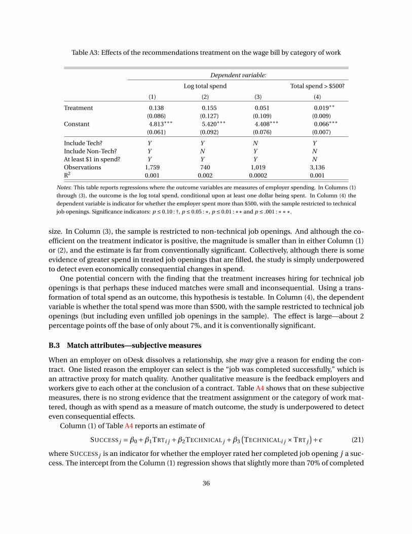
Table A3: Effects of the recommendations treatment on the wage bill by category of work

Dependent variable:

Log total spend Total spend > $500?

(1) (2) (3) (4)

Treatment 0.138 0.155 0.051 0.019∗∗

(0.086) (0.127) (0.109) (0.009)

Constant 4.813∗∗∗ 5.420∗∗∗ 4.408∗∗∗ 0.066∗∗∗

(0.061) (0.092) (0.076) (0.007)

Include Tech? Y Y N Y

Include Non-Tech? Y N Y N

At least $1 in spend? Y Y Y N

Observations 1,759 740 1,019 3,136

R2 0.001 0.002 0.0002 0.001

Notes: This table reports regressions where the outcome variables are measures of employer spending. In Columns (1)

through (3), the outcome is the log total spend, conditional upon at least one dollar being spent. In Column (4) the

dependent variable is indicator for whether the employer spent more than $500, with the sample restricted to technical

job openings. Significance indicators: p ≤ 0.10 : †, p ≤ 0.05 : ∗, p ≤ 0.01 : ∗∗ and p ≤ .001 : ∗∗∗.

size. In Column (3), the sample is restricted to non-technical job openings. And although the co-

efficient on the treatment indicator is positive, the magnitude is smaller than in either Column (1)

or (2), and the estimate is far from conventionally significant. Collectively, although there is some

evidence of greater spend in treated job openings that are filled, the study is simply underpowered

to detect even economically consequential changes in spend.

One potential concern with the finding that the treatment increases hiring for technical job

openings is that perhaps these induced matches were small and inconsequential. Using a trans-

formation of total spend as an outcome, this hypothesis is testable. In Column (4), the dependent

variable is whether the total spend was more than $500, with the sample restricted to technical job

openings (but including even unfilled job openings in the sample). The effect is large—about 2

percentage points off the base of only about 7%, and it is conventionally significant.

B.3 Match attributes—subjective measures

When an employer on oDesk dissolves a relationship, she may give a reason for ending the con-

tract. One listed reason the employer can select is the “job was completed successfully,” which is

an attractive proxy for match quality. Another qualitative measure is the feedback employers and

workers give to each other at the conclusion of a contract. Table A4 shows that on these subjective

measures, there is no strong evidence that the treatment assignment or the category of work mat-

tered, though as with spend as a measure of match outcome, the study is underpowered to detect

even consequential effects.

Column (1) of Table A4 reports an estimate of

SUCCESS j =β0 +β1TRTi j +β2TECHNICAL j +β3

(TECHNICALi j ×TRT j

)+ǫ (21)

where SUCCESS j is an indicator for whether the employer rated her completed job opening j a suc-

cess. The intercept from the Column (1) regression shows that slightly more than 70% of completed

36

Table A4: Effect of treatment on qualitative match outcomes conditional upon outcome being available

Dependent variable:

Employer rated a success? Worker-on-Employer FB Employer-on-Worker FB

(1) (2) (3)

Treatment 0.021 −0.032 0.074

(0.028) (0.061) (0.071)

Technical −0.025 0.006 0.083

(0.031) (0.066) (0.079)

Treatment × Technical −0.019 0.077 −0.099

(0.044) (0.094) (0.111)

Constant 0.714∗∗∗ 4.668∗∗∗ 4.345∗∗∗

(0.020) (0.043) (0.049)

Observations 1,770 1,541 1,436

R2 0.002 0.001 0.001

Notes: The table reports OLS regresses where the dependent variable is some employer- or worker-reported mea-

sure of match quality. In Column (1), the dependent variable is whether the employer rated the project a success

when ending the contact. In Column (2), the dependent variable is the rating (1 - 5 stars) by the worker on the em-

ployer. In Column (3), the dependent variable is the rating (1 - 5 stars) by the employer on the worker. For all three

regressions, the samples consist of filled job openings where the associated outcome measure is available. Parties

are not universally compelled to give these reports, so they are missing for some filled and ended job openings.

Significance indicators: p ≤ 0.10 : †, p ≤ 0.05 : ∗, p ≤ 0.01 : ∗∗ and p ≤ .001 : ∗∗∗.

jobs are rated as having been completed successfully. Neither the treatment assignment nor the

category of work had a detectable effect on the fraction of employers rating the project as being

completed successfully. In Column (2), the outcome variable is the worker’s feedback (1 to 5 stars)

on the employer, and in Column (3), the outcome variable the employer’s feedback on the worker.

This feedback is not required and so is not universally available for matches. In both cases, neither

the treatment group nor the job opening type had a detectable effect on the ratings.

C Predictive model of organic applicant counts

To provide a measure of expected organic applicant counts, I fit a linear model, using the lasso

(Tibshirani, 1996) for feature selection and to prevent over-fitting. I used cross-validation (Friedman

et al., 2009) to select the optimal regularization parameter. The sample included all observations

from the experiment where the job opening had at least one organic applicant.

The outcome was the log organic applicant count. The candidate predictors were: the full set

of dummies for the sub-category of the job opening (employers classify their job opening into one

of 74 mutually exclusive categories of work); the length of the job description; dummies for the the

employer’s visibility setting (employers can restrict who can see their job openings); a dummy for

whether the employer required applicants to have any past on-platform experience; a dummy for

whether the job was hourly (compared to fixed price) and a dummy for whether the job description

had an attachment. I also included all of the interactions of these predictors with themselves.

37