The Effects of Sea Level Rise on U.S. Coastal...

Originally published December 1989 by the U.S. EPA Office of Policy, Planning, and Evaluation

THE EFFECTS OF SEA LEVEL RISE ON U.S. COASTAL WETLANDS

by

Richard A. ParkManjit S. Trehan

Holcomb Research InstituteButler University

Indianapolis, IN 46208

and

Paul W. MauselRobert C. Howe

Remote Sensing Laboratory andDepartment of Geography and Geology

Indiana State UniversityTerre Haute, IN 47809

Cooperative Agreement CR814578-01

Park

The Potential Effects of Global Climate Change on the United States Appendix B: Sea Level Rise

CONTENTS

Page

ACKNOWLEDGMENTS . . . . . . . . . . . . . . . . . . . . . . . . . . . . . . . . . . . . . . . . . . . . . . . . . . . . . . . . . . . . . . . . . . . . . iii

FINDINGS . . . . . . . . . . . . . . . . . . . . . . . . . . . . . . . . . . . . . . . . . . . . . . . . . . . . . . . . . . . . . . . . . . . . . . . . . . . . . . . . 1-1

CHAPTER 1: INTRODUCTION . . . . . . . . . . . . . . . . . . . . . . . . . . . . . . . . . . . . . . . . . . . . . . . . . . . . . . . . . . . . . . 1-2CONTEXT . . . . . . . . . . . . . . . . . . . . . . . . . . . . . . . . . . . . . . . . . . . . . . . . . . . . . . . . . . . . . . . . . . . . . . . . . 1-2BACKGROUND . . . . . . . . . . . . . . . . . . . . . . . . . . . . . . . . . . . . . . . . . . . . . . . . . . . . . . . . . . . . . . . . . . . . 1-2

CHAPTER 2: METHODS . . . . . . . . . . . . . . . . . . . . . . . . . . . . . . . . . . . . . . . . . . . . . . . . . . . . . . . . . . . . . . . . . . . . 1-3DATA . . . . . . . . . . . . . . . . . . . . . . . . . . . . . . . . . . . . . . . . . . . . . . . . . . . . . . . . . . . . . . . . . . . . . . . . . . . . 1-3

Cover Classes . . . . . . . . . . . . . . . . . . . . . . . . . . . . . . . . . . . . . . . . . . . . . . . . . . . . . . . . . . . . . . . 1-3Development . . . . . . . . . . . . . . . . . . . . . . . . . . . . . . . . . . . . . . . . . . . . . . . . . . . . . . . . . . . . . . . . 1-4Elevations . . . . . . . . . . . . . . . . . . . . . . . . . . . . . . . . . . . . . . . . . . . . . . . . . . . . . . . . . . . . . . . . . . 1-4

QUALITY ASSURANCE . . . . . . . . . . . . . . . . . . . . . . . . . . . . . . . . . . . . . . . . . . . . . . . . . . . . . . . . . . . . . 1-4DESCRIPTION OF MODEL . . . . . . . . . . . . . . . . . . . . . . . . . . . . . . . . . . . . . . . . . . . . . . . . . . . . . . . . . . 1-5

Inundation Model . . . . . . . . . . . . . . . . . . . . . . . . . . . . . . . . . . . . . . . . . . . . . . . . . . . . . . . . . . . . 1-5Spatial Model . . . . . . . . . . . . . . . . . . . . . . . . . . . . . . . . . . . . . . . . . . . . . . . . . . . . . . . . . . . . . . . . 1-5

CHAPTER 3: SIMULATIONS AND SYNTHESIS OF RESULTS . . . . . . . . . . . . . . . . . . . . . . . . . . . . . . . . . . . 1-11CASE STUDY: LONG BEACH, NEW JERSEY . . . . . . . . . . . . . . . . . . . . . . . . . . . . . . . . . . . . . . . . . . 1-11NATIONAL IMPACTS . . . . . . . . . . . . . . . . . . . . . . . . . . . . . . . . . . . . . . . . . . . . . . . . . . . . . . . . . . . . . . 1-14REGIONAL TRENDS . . . . . . . . . . . . . . . . . . . . . . . . . . . . . . . . . . . . . . . . . . . . . . . . . . . . . . . . . . . . . . . 1-21

Mid-Atlantic . . . . . . . . . . . . . . . . . . . . . . . . . . . . . . . . . . . . . . . . . . . . . . . . . . . . . . . . . . . . . . . 1-21Southeast . . . . . . . . . . . . . . . . . . . . . . . . . . . . . . . . . . . . . . . . . . . . . . . . . . . . . . . . . . . . . . . . . . 1-21West Coast . . . . . . . . . . . . . . . . . . . . . . . . . . . . . . . . . . . . . . . . . . . . . . . . . . . . . . . . . . . . . . . . . 1-39Northeast . . . . . . . . . . . . . . . . . . . . . . . . . . . . . . . . . . . . . . . . . . . . . . . . . . . . . . . . . . . . . . . . . . 1-39

CHAPTER 4: SUMMARY . . . . . . . . . . . . . . . . . . . . . . . . . . . . . . . . . . . . . . . . . . . . . . . . . . . . . . . . . . . . . . . . . . 1-51

REFERENCES . . . . . . . . . . . . . . . . . . . . . . . . . . . . . . . . . . . . . . . . . . . . . . . . . . . . . . . . . . . . . . . . . . . . . . . . . . . . 1-53

Park ii


ACKNOWLEDGMENTS

This project was made possible by many individuals who often worked overtime to obtain the results in a timely manner. At Indiana State University, Drs. Richard Hyde and Kamlesh Lulla were involved in the development of methods used in the analysis of remotely sensed data, with programming support from Nicholas Vesper and Norman Levine; analysis of. Landsat data and digitization of elevational data were performed by Randy Pearson, Robert Regis, Timothy Gress, Mao Chang, Huen Chen, Mark Jakubauskas, David Kettler, Steven Kopp, Asilah Mahmud, Chenyge Mao, Mark Karaska, Kai Huang, and Jae Lee. At Butler University, Michael Magier assisted in the development of software; assistance in editing data, performing simulations, and preparing results was given by Julie James, Michael Yamanichi, Lisa Guendling, and Joseph Poston; manuscript editing and review was provided by James Rogers, Thomas Armentano, Paul van der Heijde, and Orie Loucks. The manuscript benefited from the suggestions of Joy Zedler, Thomas Cavinder, the U.S. Fish and Wildlife National Coastal Ecosystem Team, and an anonymous reviewer. The project was funded through Cooperative Agreement CR814578-01 with the U.S. Environmental Protection Agency; James Titus was the project monitor.

Park iii


Park iv


FINDINGS1

During the next century, rising sea level due to global warming will have a profound impact on the coastal wetlands of the United States and a significant impact on coastal lowlands. With an almost-certain rise of a half-meter by the year 2100 and with all currently developed areas protected from inundation and erosion, more than 4,000 Mi2 of vegetated wetlands will be lost. With a probable rise of 1 meter by the year 2100, 6,441 mi2 or approximately 65% of the coastal marshes and swamps of the contiguous United States could be lost. With a 2-meter rise, 7,423 Mi2 or 77% of the coastal wetlands of the contiguous United States could be lost, and remaining southeastern marshes could be converted to mangrove swamps. Furthermore, unprotected barrier islands would be lost through accelerated beach erosion; much of the Florida Everglades and Keys would be inundated; and low-lying coastal cities such as Charleston, South Carolina, and Long Beach, Mississippi, could be submerged if not ringed by dikes. In a worst-case scenario, with a 3-meter rise and all dry land protected from inundation, 10,953 mi2 of marshes and swamps could be lost.

1 Although the information in this report has been funded wholly or partly by the U.S. Environmental Protection Agency under Cooperative Agreement CR814578-01, it does not necessarily reflect the Agency's views, and no official endorsement should be inferred from it.

Park 1-1


CHAPTER 1

INTRODUCTION

CONTEXT

The "greenhouse gases" -- carbon dioxide, methane, nitrous oxides, and chlorofluorocarbons that are transparent to sunlight but absorb reradiated heat energy -- are increasing at an alarming rate due to human activities. CO2 and other greenhouse gases may double by the year 2030 as compared to the amounts present at the start of the. industrial revolution (Villach, 1985), warming the earth7s surface between 2 and 4�C (Titus and Seidel, 1986). If the average temperature increases by YC by 2050 and remains constant thereafter, sea level will probably rise approximately 1 meter (in) by 2100; a global warming of 6'C by 2100 could result in a sea level rise of 2.3 in (Thomas, 1986).

Such an accelerated rise in sea level would have a serious impact on the distribution of U.S. coastal wetlands. Salt, brackish, and fresh marshes -as well as mangrove and other swamps would be lost due to inundation and erosion, or would migrate inland as adjacent lowlands not protected by engineering structures are inundated. The value of these wetlands as habitat for wildlife would be impaired, and their biodiversity would decrease. Although many wetlands have kept pace or have increased in area with historic sea level rise due to sediment entrapment and peat formation (Davis, 198S), vertical accretion of wetlands has not been observed to occur at. rates comparable to those projected for sea level rise in the next century. In fact, the rate of a 1-m rise by the year 2100 will be equal to that attained during the disintegration of the continental ice sheets at the end of the Pleistocene (Peltier, 1988), which drowned barrier islands and associated features on the continental shelves.

Wetlands are vital to the ecology and economy of U.S. coastal areas. Their biological productivity is equal to that of any other natural or agricultural system (cf. Teal, 1962; Ryszkowski, 1984). Although little of that productivity may be available to marsh animals and coastal fisheries (Montague et al., 1987), over half the species of commercially important fishes in the southeastern United States use salt marshes as nursery-grounds (Thurman, 1983). Wetlands also remove pollutants (Pope and Gosselink, 1973) and provide, protection from floods, storms, and high tides (Lugo and Brinson, 1978). Based on these functions, it has been estimated that marshes provide an annual return to society equivalent to $5,500/acre (Thurman, 1983). For these and other reasons, the Congress and the U.S. scientific community are seeking the best quantitative estimate of potential impacts on coastal wetlands under various scenarios of sea level rise and coastal zone management policy.

BACKGROUND

Previous studies by EPA indicated the scope of the problems associated with sea level rise (Barth and Titus, 1984; Titus 1986, 1988) and showed that a more detailed study was warranted. As a part of one of these previous studies, Holcomb Research Institute developed a simulation model (SLAMM) that was used to conduct preliminary regional analyses of the effects of sea level rise on U.S. coastal wetlands. The original model was based on manually coded data on elevation and cover classes from topographic maps, using a 1-km2 grid (Park et al., 1986ab; Armentano et al., 1988). Simulations suggested that large areas of coastal wetlands would be lost with sea level rise. However, both data and the model needed refining if the results were to be used for evaluating policy. The objective of the present study, therefore, is to present and document the refined databases and calculation procedures, and their limitations, together with improved estimates as to how much of the nation's coastal wetlands are likely to be lost under various scenarios of sea level rise.

Park 1-2


CHAPTER 2

METHODS

DATA

Ninety-three sites were chosen, using an unbiased systematic sampling of U.S. Geological Survey topographic maps at a scale of 1:24,000. Starting with the easternmost quadrangle in Maine and restricting the choice to those maps that included some part of the coast, every 15th quadrangle was picked as the center of a site consisting of one to four quadrangles. (Two sites are represented by 1:64,000 maps and two by 1:25,000 maps.) Of these, a subsample of 46 sites was used in this initial study- Four supplemental sites were also chosen for verification purposes. For most coastal sites with low slopes and extensive lowland and wetland areas, a cell size of 500 in by 500 in was used; this is an area of 25 hectares (ha) or 61.75 acres; with this coarse-grained resolution, a site typically contained four quadrangles. For sites with steep slopes or heterogeneous urban development, a fine-grained resolution of 250 in by 250 in (6.25 ha or 15.44 acres) was used; normally such a site was restricted to one quadrangle. A normal coarse-grained site contains as many as 3,400 cells; some sites with fine-grained resolution and covering four quadrangles contain almost,14,000 cells.

Each cell is represented by information on elevation, percent cover in various classes, development, and presence of protective engineering structures. Eleven cover classes were distinguished, including upland (above 12 ft or 3.66 m elevation); lowland (above mean high water spring tide level [MHWS] and below 3.66 in elevation); sandy area (usually backshore and dunes areas, but including both lowland and upland areas characterized by exposed sand); freshwater marshes, saltmarshes, freshwater swamps, mangrove swamps, combined beaches and tidal flats, rocky intertidal areas, and water.

Cover Classes

The cover-class data were obtained by analysis of multispectral Landsat data from essentially cloud-free, geocorrected scenes, augmented by visual interpretation of high-altitude color-infrared photographs (with a scale of 1:58,000). Numerous studies have shown that these forms of remote sensing can effectively differentiate wetland and other coastal cover types (Estes and Thorley, 1983).

Well-established methods for quantifying remotely sensed cover-class data were used (Mausel, 1985). The HINDU algorithm (Dasarthy, 1974) was used to partition the spectral data into classes of repetitive signatures for a particular site. Usually 20 to 30 clusters were obtained. These were combined by an experienced analyst to represent the cover classes on the basis of cluster statistics and spectral signatures, confirmed by information from the maps and photographs. The correspondence between pixels in combined clusters and a designated cover class, such as low marsh, is not perfect. Preliminary analyses of selected sites suggest that accuracies for well-defined classes range from 75 to 95+ percent. Features represented by mixed pixels or by ambiguous spectral responses pose a problem. Residential and commercial developments were not identified from the spectral data because pavement and roofs could be confused with the “sandy area” class. However, because of the need to identify all wetlands, the swamp class was used despite an ambiguous signature. Where possible, high and low marshes were distinguished,. based on “dry” and “wet” spectral signatures.

Each Landsat pixel represents an area S7 in by 79 in. The data were resampled and aggregated to form pixels with an area of 71 in by 63 in, and were printed at a scale of 1:24,000 to facilitate comparison with topographic maps. Thus with a 500-m by 500-in grid, the unit cell contains 55 + pixels. The percent cover for each class was stored and reported in increments of 5%.

In the absence of "ground truth" based on detailed field checking, the cover determinations for any particular site should be considered best-estimates consistent with the regional goals of the study. Topographic maps and USFWS National Wetland Inventory (NWI) maps were used to confirm the interpretations. Because the Landsat imagery is often from 1986 and 1987 and supersedes map coverage by a significant number of years, the spectral signatures were often

Park 1-3


accepted in the event of conflict. For example, at a New Jersey site both the topographic map, photorevised in 1972, and the NWI map, based on 1977 aerial photography, showed an extensive unbroken marsh; however, the Landsat imagery and the high-altitude photograph provided unmistakable evidence that a large area had been converted to lowland (probably with dredge fill). Marshes, shadowed uplands, and uplands with redwoods sometimes exhibited similar spectral signatures; these were reassigned manually on the basis of topographic maps. Swamps proved to be difficult to distinguish from upland forest; a dense tree canopy can effectively mask any standing water. For several sites swamps were reassigned manually, based on topographic maps. Because sandy areas often included beaches and tidal flats, these wetlands are underestimated in the data, and a transient response is often observed in the simulations as the model reapportions sandy area to beach.

Development

Residential and commercial developments were identified from topographic maps. If a cell contained sufficient buildings and other structures worthy of protection (including airports and wharves), the cell was characterized as developed. Because the maps are older than the Landsat data and the simulations start with the Landsat coverage, this underestimates the extent of development and subsequent protection. Although it would be of interest to simulate continued coastal development, that is beyond the scope of this study.

Elevations

Topographic elevations on U.S. Geological Survey maps are relative to the 1929 sea level, known as the National Geodetic Vertical Datum (NGVD); therefore, elevations of the dry-land classes (upland, lowland, and sandy area) were corrected for historic sea level rise from 1929 to the date of the topographic map. The long-term value of 1.2 mm/yr was used for historic sea level rise.

Dry-land elevations were further corrected for changes from the map date to the date of Landsat coverage, at which time the areas of the classes were observed. This correction is based on both the 1.2 mm/yr trend and observed subsidence due to regional isostatic adjustments and -tectonics, and local compaction due to withdrawal of water, oil, and gas.

The elevational data were obtained by digitizing the corner elevations of each cell, based on interpolations of elevations from the topographic maps. Both the elevational and the Landsat data were recorded using the Universe Transverse Mercator grid and were combined for each cell in the site data file. Elevations and elevational ranges for classes within a cell were apportioned based on an algorithm that assumes sandy and rocky areas to have a convex profile, and other lowland and upland areas to have a concave profile. An elevational mosaic was assumed for saltwater wetlands, with each cover class traversing its full elevational range within a cell (representing the usual microtopography that occurs with small tidal flats and beaches, tidal creeks, natural levees, and back-levee areas). Saltwater wetland elevational ranges were computed by assuming constant relationships of the wetlands to tidal datums (cf. Lefor et al., 1987), with mean or half tide level (MTL) as 0; beach and tidal flats extending from mean low water (MLW) to mean high water (MHW), or from MLW to MTL on coasts with low wave energy and- vegetated wetlands; low marsh extending from MTL to MHW; high marsh extending from MHW to MHWS; and mangrove swamps extending from MTL -to MHWS. (Occasionally saltwater wetlands occur above MHWS, but the area is small and can be ignored.)

QUALITY ASSURANCE

Quality assurance, mandated by the EPA Administrative Procedures Act, received close attention in this study. All interpretations and implementations received an independent evaluation by another member of the study team, and records have been kept for all procedures.

Selected sites were visited by the principal investigator and members of the remote sensing team. This helped provide ground truth for representative sites and promoted inclusion of subtle relationships in the model. Discussions of the modeling study were held at several coastal wetland labs, and suggestions for improving the study were solicited.

Park 1-4


DESCRIPTION OF MODEL

Stated simply, the objective of the modeling undertaken in this study has been to consider the dominant processes involved in vegetative wetland conversions and related shoreline reconfigurations during long-term sea-level rise. The model, SLA.MM2, differs from other wetland models (pay et al., 1973; Wiegert et al., 197S; Hopkinson and Day, 1977; Browder et al., 198S; Sklar et al., 198S; Costanza et al., 1987; Kana et al., 1988) by its ability to predict map distributions of wetland cover under conditions of accelerated sea level rise,and by its applicability to the diverse wetlands of the contiguous coastal United States.

Eleven cover-classes were modeled in each of over 3,000 cells for 115 or more years; therefore, the level of scientific detail represented had to be balanced with efficient computational algorithms. The following sections present the basic constructs for each of the processes considered in order to establish the basis for the model results; the constructs are organized in two sections, the basic inundation model and-the map-based spatial model. Simplifying assumptions that may bias the results, and could be investigated more fully in the future, are emphasized by italics.

Inundation Model

The colonization of newly inundated dry land by wetland vegetation and loss of wetlands due to further inundation is based on a straightforward geometric relationship, with lag effects for some conversions. Seven processes are considered as part of the inundation model.

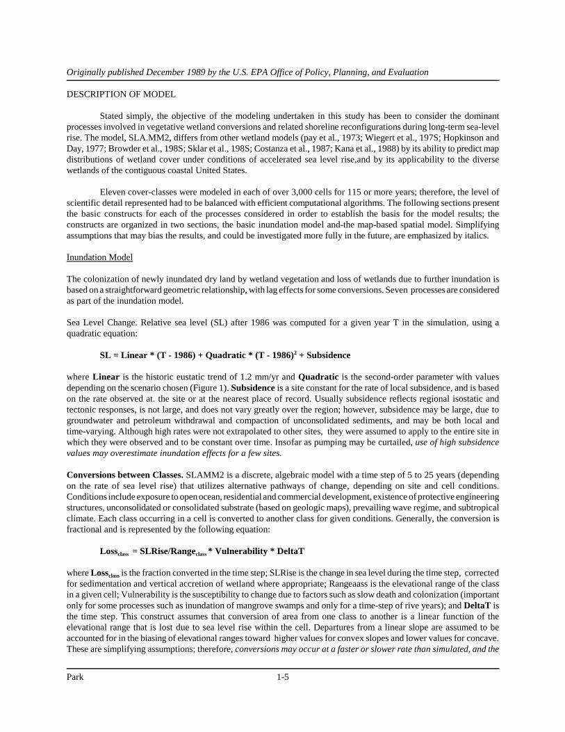
Sea Level Change. Relative sea level (SL) after 1986 was computed for a given year T in the simulation, using a quadratic equation:

SL = Linear * (T - 1986) + Quadratic * (T - 1986)2 + Subsidence

where Linear is the historic eustatic trend of 1.2 mm/yr and Quadratic is the second-order parameter with values depending on the scenario chosen (Figure 1). Subsidence is a site constant for the rate of local subsidence, and is based on the rate observed at. the site or at the nearest place of record. Usually subsidence reflects regional isostatic and tectonic responses, is not large, and does not vary greatly over the region; however, subsidence may be large, due to groundwater and petroleum withdrawal and compaction of unconsolidated sediments, and may be both local and time-varying. Although high rates were not extrapolated to other sites, they were assumed to apply to the entire site in which they were observed and to be constant over time. Insofar as pumping may be curtailed, use of high subsidence values may overestimate inundation effects for a few sites.

Conversions between Classes. SLAMM2 is a discrete, algebraic model with a time step of 5 to 25 years (depending on the rate of sea level rise) that utilizes alternative pathways of change, depending on site and cell conditions. Conditions include exposure to open ocean, residential and commercial development, existence of protective engineering structures, unconsolidated or consolidated substrate (based on geologic maps), prevailing wave regime, and subtropical climate. Each class occurring in a cell is converted to another class for given conditions. Generally, the conversion is fractional and is represented by the following equation:

Lossclass = SLRise/Rangeclass * Vulnerability * DeltaT

where Lossclass is the fraction converted in the time step; SLRise is the change in sea level during the time step, corrected for sedimentation and vertical accretion of wetland where appropriate; Rangeaass is the elevational range of the class in a given cell; Vulnerability is the susceptibility to change due to factors such as slow death and colonization (important only for some processes such as inundation of mangrove swamps and only for a time-step of rive years); and DeltaT is the time step. This construct assumes that conversion of area from one class to another is a linear function of the elevational range that is lost due to sea level rise within the cell. Departures from a linear slope are assumed to be accounted for in the biasing of elevational ranges toward higher values for convex slopes and lower values for concave. These are simplifying assumptions; therefore, conversions may occur at a faster or slower rate than simulated, and the

Park 1-5


Park 1-6


simulations should be considered as approximate responses to be expected for different scenarios and should be used primarily for computing regional averages.

Tropical Conditions. The conversion of dry land to wetland vegetation is complicated by global climate change. Mangroves are limited to those areas without appreciable frost. At present, viable populations of small black mangroves occurs far north as Daytona, Florida, and in the Mississippi River delta and along the barrier islands of the northern Gulf of Mexico (Sherrod and McMillan, 1985). With only a slight decrease in killing frosts, these populations could spread to other coastal areas where adjacent water moderates the climate. The SLAMM2 simulations assume that for all scenarios other than a continuation of the current sea-level trend, mangrove swamps can become established in the northern Gulf of Mexico and Atlantic coast of Florida beginning in the year 2000. They are assumed to grow in Georgia and South Carolina at slightly later dates. This is an approximation and could be sharpened by using projected climatic changes for each area of the coast.

Coastal Engineering Structures. The presence of dikes and levees completely enclosing coastal areas was noted from the topographic maps. The two protection scenarios represent further construction of dikes around all developed areas and all dry land, respectively. Areas so protected are not allowed to convert to other classes in the simulations. Enclosed wetlands are assumed to be m6intained'in their initial condition.

Death and Colonization. Death and conversion of low marsh to water by inundation and corresponding conversion of high marsh to low marsh are assumed -to occur at a linear rate of 20% per year of the potential based on inundation alone (Vulnerability = 0.2); with Ei normal time step of five years or more, this produces no discernible lag. However, in the model, mangrove swamps are converted to water at the rate of 10% per year of the potential, producing a 50% lag for a time step of five years. Because they are intolerant to saltwater, freshwater swamps and marshes are converted instantaneously to water or high marsh, respectively, or to mangrove swamp if subtropical.

Inundated lowlands and sandy areas are instantaneously converted to either high marsh or mangrove swamp by the model. This assumes colonization to proceed faster than the normal five-year time step, and it assumes that paved surfaces are a negligible impediment to colonization. Although relatively rapid colonization rates have been reported for some areas, these assumptions may lead to an overestimate of vegetated wetlands.

Sedimentation and Accretion. One of the pervasive challenges in developing the model was to incorporate processes with variable rates known from studies in different areas but not known for the specific study sites. Perhaps the most important process is vertical accretion of wetlands. In the past in many areas, accretion has kept pace with local changes in sea level. Although accretion rates vary widely at particular locales and among areas, including most of the study sites, a pattern emerges that can be used in estimating local rates. In deltaic areas characterized by extensive marshes, 10 mm/yr seems to be representative, although much higher maximal values have been observed; in many areas with moderately extensive wetlands, 5 mm/yr seems to be a common midrange value; in areas with little wetland development, 2 mm/yr seems to be a representative minimal value (cf. Letzsch and Frey, 1980; Gosselink, 1984; Armentano et al., 1988). Therefore, as a simplifying assumption, if the percentage of salt wetlands at the start of the simulation is greater than or equal to 30%; an accretion rate of 10 mm/yr is used for low marsh at the site; if greater than 5% and less than 30%, an accretion rate of 5 mm/yr is used; if less than or equal to 5%, an accretion rate of 2 mm/yr is used. Because marsh areas that are back from water courses tend to have accretion rates that are approximately half those of streamside marshes (cf. Gosselink, 1984), the values are, halved for high marsh. Areas enclosed by dikes are not affected by these accretion rates because the marshes are not permitted to change.

Rates of accretion in mangrove swamps seem to depend more on extremely localized conditions and have not been well studied. In a detailed study of a mangrove swamp in Australia, Bird (1986) reported rates varying from 2 to 13 mm/yr. We have assumed 5 mm/yr to be representative and have used that value for all areas with mangroves.

The assumption of an accretion rate for a particular wetland type that is uniform over a site and constant through time probably leads to an overestimate of wetland maintenance.

Park 1-7


Sedimentation rates in adjacent areas of sheltered water have not been well documented, nor are they as important as accretion; therefore, the local sedimentation rate for areas of sheltered water is taken to be one-tenth that of accretion. Admittedly this is an arbitrary value, but the model is not sensitive to it.

Few U.S. beaches are currently prograding or expanding due to sedimentation. The model assumes that progradation of exposed beaches and tidal flats occurs only under conditions of high sedimentation and a continuation of historic sea level rise. If sedimentation exceeds sea level rise, under. any scenario, areas of sheltered water are converted to tidal flats which in turn are converted to wetlands, using the following relationships:

Losswater = (DeltaT * Sedimentation - SLRise)/Depth LossTidalflat = (DeltaT * Sedimentation - SLRise)/RangeTidalflat

where Losswater is the fraction of area of water converted to tidal flat during the time step DeltaT; Sedimentation is the rate of sedimentation (m/yr); SLRise is the change in sea level during the time step; Depth is the average depth of sheltered water; and RangeTidalflat is the elevational range of tidal flats at the site. The construct treats the fractional losses as uniform for all cells with sheltered water and tidal flats, and it ignores subsidence; therefore, it probably overestimates progradation at sites with high sedimentation rates (as indicated by extensive initial wetlands) for the scenario of continued historic sea level rise.

Salinity. Salinity is not explicitly modeled. This has two consequences in the simulations: low-lying freshwater marshes may be designated as saltmarshes, and salt pannes and tidal flats in arid regions may be predicted to convert to saltmarshes, on the basis of elevation.

Spatial Model

In addition to the effects of inundation represented by the simple geometric model described above, second-order effects occur due to changes in the spatial relationships among the coastal elements. Accordingly, SLAMM2 incorporates a map-based model component to consider four spatially important processes: coastal beach erosion, overwash, barrier breaching, and headland erosion..

Erosion. Under equilibrium conditions, erosion and deposition balance and wetlands are not lost. However, even historic sea level rise coupled with local subsidence has upset coastal equilibrium in many parts of the world (Bird, 1986; Bruun, 1986). Although the processes of erosion can be expressed by detailed quantitative relationships, such an approach is beyond the scope of the present study. Rather, qualitative relationships are defined and used as thresholds for including constant rates of wave erosion in simulating the localized loss of wetlands. The effects of severe storms are included in these average values. The model can represent several levels of erosion based on the observed average fetch (the distance across which wind-driven waves can be formed) of shelte *red water. These levels are represented by scalars: "none," "little," "moderate," "heavy," and "severe"; however, in the present implementation, constant erosion is triggered only when the erosional scalar is greater than "moderate," which occurs when the average fetch exceeds 9 km. This occurs at only a few sites.

The model also recognizes exposure to open ocean as triggering erosion of wetlands. Cells can become exposed as protective barrier islands and spits are breached. If a saltmarsh is exposed to the open ocean or erosion is greater than "moderate," 0.4% of the marsh is lost per year (2 m/yr using a SOO-m grid). If a swamp is exposed to the open ocean or erosion is greater than "moderate," 0.2% of the swamp is lost per year (I m/yr using a 500-m grid). These values are based on the literature (Hall et al., 1986) and on rates observed from photorevised and sequential maps of areas with eroding wetlands.

Bruun (1962, 1986) has shown that on the, average, recession of beaches and backshore areas is one hundred times the change in sea level. Assuming a beach slope of 12*, an average for many beaches (cf. Dyer 1986), the width is rive times the height (tan 1T = 0.2). Therefore,

Park 1-8


Recession = 100 * SLRise

WidthBeach = 5 * RangeBeach

LossBeach = Recession/WidthBeach

where Recession is the width of beach lost during a time step (in); SLRise is the change in sea level (in) during the time step; WidthBeach is the theoretical width of the beach (in); RangeBeach is the elevational range of the beach (MHWS-MLW in in); and Loss each is the fraction of beach lost during a time step.

Assuming that beach width is maintained at the expense of any adjacent backshore and dune area, and assuming that the beach runs the length of the cell (an assumption that probably results in an overestimation of beach area), then

AreaBeach = WidthBeach * Scale/10,000

RecessionSandyArea = AreaBeach - AreaBeach

while there is a deficit of beach and there is sandy area to be eroded; if the "protect backshore" scenario is chosen, recession is not allowed. AreaBeach is the theoretical area of beach (ha), given equilibrium conditions; Scale is the grid size, usually either 500 or 250 in; 10,000 is a proportionality constant to convert meters to hectares; Recession SandyArea

is the sandy area converted during the time step (ha); and AreaBeach is the area of the beach before conversion of adjacent sandy area (ha).

Beaches that are developed are assumed to be protected; therefore, developed backshores are not allowed to erode in the simulations unless a "no,protection" scenario is chosen. However, no provision is made for active formation of natural and artificial dunes on undeveloped beaches, nor is natural nourishment of beaches due to eroding headlands simulated. Therefore, the model probably overestimates beach erosion on exposed, undeveloped coasts.

Overwash. As erosion of backshore and dune areas occurs and as other lowlands are drowned, wetlands on the lee side of coastal barriers are subject to conversion due to overwash, the process by which sediments are carried over the crest of the barrier and deposited onto adjacent wetlands. This process is simulated only for areas having a beach and only during the time step in which the lowland -is breached. It assumes that 50% of the adjacent high marsh, 25% of the low marsh, and 5% of mangrove (if present) in the adjacent cell is converted to beach and tidal flat; the percentages are educated guesses based on observations of existing overwash areas (cf. Leatherman and Zaremba, 1986). Adjacent water is converted to beach and tidal flat by an amount based on the assumption that upper beach sediments (occurring between mean tide level and mean high water spring tide level) are transported into the water:

LossWater = (MHWS - MTL)/Depth

where LossWater is the fraction converted.

Exposure to Open Ocean. Breaching of coastal barriers results not only in overwash but also in exposure of areas to the open ocean. At the beginning of the simulation, the model changes cells from unexposed to exposed if they are in line, based on prevailing wave direction, with exposed water and without intervening areas other than water. Each time overwash occurs, cells on the tee side are changed to exposed, and with each time step the adjacent cell on the lee side is changed to exposed if that cell is all water. This effectively limits erosion in the once-sheltered water areas and mimics the continuation of shoal-water conditions.

Erosion of Headlands. Erosion of sandy areas is simulated to maintain equilibrium with adjacent beaches; but erosion of lowlands and uplands that do not have a multispectral signature indicating sand is not simulated. Therefore, recession of sandy areas is probably overestimated by the model, but erosion of other dry lands is ignored.

Park 1-9


In summary, the model probably errs slightly toward maintenance of wetlands and toward accelerated loss of barrier islands, but overall it provides prudent forecasts useful in guiding policies for coping with sea level change.

Park 1-10


CHAPTER 3

SIMULATIONS AND SYNTHESIS OF RESULTS

As would be expected from the major differences in coastal physiography around the United States, the potential for loss of wetland resources due to a rise in sea level varies widely from region to region. Thus, balanced sampling was required for both the regional and national estimates of losses. Each site was chosen using an unbiased sampling procedure (see DATA) and covers an area from the open ocean to uplands (or diked lowlands) so that both loss and migration of wetlands can be evaluated. The standard set of simulations for each site spans a period from the date of the remote imagery to the year 2100 and provides estimates of response to:

– a projection of the historic trend of sea level rise (1.2 mm/yr) (resulting in a eustatic sea level stand of 0.14 in above 1986 level by the year 2100); and 1/2-, 1-, 2-, and 3-meter sea levels by the year 2100

– no protection of dry lands, protection of backshore areas of beaches only, protection of all developed areas, and protection of all dry land (including enclosed wetlands)

The sea level scenarios are based on projections given by Thomas (1986), assuming different global-warming scenarios and the possible melting of glacial ice and thermal expansion of the upper layers of the oceans. The 1-meter scenario is considered most probable in the absence of significant efforts to curb global warming. The protection scenarios are intended to represent different levels of defending coastal areas from inundation and erosion. With the "no protection" scenario, only those areas already protected by levees and dikes will be protected in the future. The "protect backshore" scenario proved to be uninteresting and was not used in the summaries; it was intended to represent the protection of backshore areas (especially on barrier islands) through sand nourishment and bulkheads, without protection of adjacent lowlands. Protection of developed areas represents the effects of enclosing all existing developed areas (see DATA) with dikes and levees; it is conservative in that further development is not considered. The extreme scenario is protection of all dry land; note that this can lead to protection of freshwater wetlands that are landward of dry land.

CASE STUDY: LONG BEACH, NEW JERSEY

One case study is presented here to illustrate the level of resolution sought in the database, in the simulation of changes over time, and in the computational and summarization procedure. Long Beach Island, New Jersey, and the adjacent bay and low-lying mainland comprise a typical barrier island system to the south of Atlantic City (Figure 2). The data analysis and simulations of this site provide both insights into, and limited verification of, the SLAMM2 algorithms.

Examination of the map shows undeveloped and developed dry land, saltmarsh, swamp, and water (Figure 3). An enlarged portion of the map (Figure 3B) shows the 5W-m by 500-m cells formed by aggregation of classes from the unsupervised classification of the Landsat multispectral data, represented by the pixel map (Figure 3Q. Interpretation of the Landsat data was facilitated by comparison with the high-altitude infrared photograph of the same area (Figure 3D). The elevations and locations of developed areas were obtained from the topographic map (Figure 3E). The National Wetland Inventory map (Figure 3F) was used to confirm the interpretations of the classes.

Detailed examination of the maps demonstrates two problems. Only the dominant class is plotted in the computer-generated map (Figure 3A,B); therefore, some of the islands are not shown because the cells happened to cover more water than marsh. Also, the swamp in the northwestern corner of the site probably includes forested upland.

Park 1-11


Park 1-12


Park 1-13


The impact of sea level rise perhaps is best visualized by maps representing different scenarios of sea level rise, with and without protection of developed areas (Figure 4). Marsh persists with a 14-cm rise in sea level by the year 2100, although a significant area of swamp is lost by inundation (Figure 4B); more likely, some of the area presently covered by swamp will slowly be converted to saltmarsh, but that transfer is not simulated. With a 0.5-m rise by the year-2100, most marsh is lost (Figure 4Q. There is little change with 1-, 2-, and 3-m rises when developed areas are protected (Figure 4D-F); however, without protection, saltmarsh would be free to migrate onto the unpaved areas of developed lowlands such as those west of Ship Bottom (cf. Figure 4G), and with 2- and 3-m rises Long Beach Island would be breached (Figure 4H,I).

The gradual changes in cover and decline of wetlands with sea level rise are portrayed most effectively by an area graph (Figure 5). It is apparent that wetlands will be lost rapidly with any sea level rise greater than the historic trend; furthermore, almost all saltmarsh is lost by the 2080 when an 0.8-m rise is reached, using the most probable scenario of 1 m by the year 2100.

This projection is quite different from that of Kana et al. (1988) based on detailed transects and application of a simple geometric model. They concluded that essentially no wetland would be lost by 2075, given the 1-m scenario. Examination of their composite transect for the area (Figure 6) shows why their results are so different. They used two feet as the tidal range, whereas we used one foot, as reported on the Long Beach topographic map; but, more important, the marsh zones are displaced well above normal levels relative to the tidal range (equivalent to that expected for a 5-foot tidal range). Kana et al. (1985) attribute this to alteration of the hydrology by mosquito ditches,-, however, it is possible that the same regional hydraulic gradient that promotes the adjacent swamps is responsible for maintaining wetter conditions than would be expected from tidal conditions alone. Compounding the discrepancy in predictions, we interpreted the marsh to be low based on a “wet” spectral signature, whereas Kana et al. (198S) found that high marsh dominated (Figure 6). We were unable to duplicate their projection of no marsh loss by imposing a S-foot tidal range with high marsh instead of low. They assumed a uniform sedimentation and accretion rate of 5 mm/yr, compared to our assumption of 5 mm/yr for low marsh, 2.S mm/yr for high marsh, and none for adjacent lowland; however, varying the accretion rate of low marsh from 2 mm/yr to 10 mm/yr only changed the timing of the loss of saltmarsh predicted by SLAMM2 by approximately 17 years (Figure 7). It is difficult to reach any conclusions from this attempted verification, but it.is quite possible that our projection of total loss of marsh is more realistic, given the tendency for flooding.

NATIONAL IMPACTS

Although losses are highly variable around the U.S. coastline, the most important estimates are those for the nation as a whole. Simulations for 98 sites are planned, but for this initial analysis an unbiased subsample of 46 sites has been used. These sites represent a broad spectrum of temperate and subtropical coastal types, with varying tidal ranges, subsidence and accretion rates, fetches, and degrees of development (Table 1).

The percent coverage of the coastline with these 46 sites was used to estimate the initial area of wetlands, as well as the areas projected to be lost under the different sea-level scenarios. For example, the 29 sites in the mid-Atlantic subsample represent 8.62% of the area of the Mid Atlantic as defined in this study; the reciprocal of that value yields a transformation factor of 11.6, which was used to scale the subsample results to the entire Mid Atlantic. These calculations yield a national estimate of 13,145 mi2 of coastal wetlands in 1986 (the time of Landsat coverage for the respective sites), compared to the estimate of 14,723 for comparable wetlands as reported by Titus and Green in this volume. (The wetlands for the mid-Atlantic and West coasts are underestimated in this initial study.)

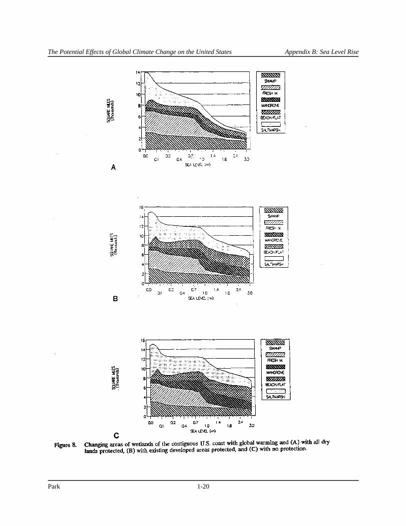
In Figure 8 the independent variable, time, has been replaced by sea level, making the ordinate more general but causing it to be expressed on an exponential scale. Mindful of the nonlinearity, saltmarshes are seen to expand initially and then decline by approximately 2,000 mi2 with a 0.1-m rise in sea level in all three protection scenarios; this decline is due to the predicted rapid loss of saltmarshes in Louisiana and the rest of the northern Gulf of Mexico. With all dry land protected, salt marshes will continue to decline until almost all disappear with a 3-m rise, and mangrove swamps will not change significantly in area; with only developed areas protected, the decline of saltmarshes will be much less pronouced, and mangrove' swamps will increase significantly; with no protection, saltmarshes will decline

Park 1-14


Park 1-15


Park 1-16


Park 1-17


Park 1-18


Table 1. Study site locations, tidal range, subsidence, sedimentation and accretion rates, and fetch for the sites used in the initial study.

Site Latitude Longitude Ocean tide (m)

Inland tide (m)

Subsidence (mm/yr)

Sedimentatio n (mm/yr)

Accretion (mm/yr)

Fetch (km)

NORTHEAST MEROCKLA. Rockland 44 07’30 69 07’30 2.8956 2.8956 1 0.20 2.0 3 MAMARBLE. Marblehead 42 37’30 70 52’30 2.7737 0 1.7 0.20 2.0 0 MAWESTPO. Westport 41 37’30 71 07’30 0.9144 0.9144 1.5 0.20 2.0 1 RIWATCHH. Watch Hill 41 22’30 71 52’30 0.7924 0.7924 0.6 0.20 2.0 1 CNBRIDGE. Bridgeport 41 15’ 73 15’ 2.0726 2.0726 0.9 0.20 2.0 1

MID ATLANTIC NYPATCHO. Patchogue 40 52’30 73 07’30 0.7924 1.1828 1.5 0.20 2.0 6 NJLONGBE. Long Beach 39 45’ 74 15’ 0.9144 0.3048 2.7 0.50 5.0 3 DEREHOBA. Rehoboth B. 38 45’ 75 07’30 0.3657 0.0609 1.9 0.20 2.0 4 MDEASTON. Easton 38 52’30 76 07’30 0 0.3048 2.4 0.20 2.0 1 MDELKTON. Elkton 39 37’30 76 00’ 0 0.7924 2.1 0.20 2.0 2 VABLOXOM. Bloxom 37 52’30 75 37’30 1.0972 1.0972 1.9 0.20 2.0 1 VANEWPOR. Newport News 37 07’30 76 30’ 0.762 0.8534 3.1 0.50 5.0 5

SOUTH ATLANTIC NCENGELH. Engelhard 35 45’ 76 07’30 0 0 0.6 0.20 2.0 2 NCLONGBA. Long Bay 35 00’ 76 30’ 0.9144 0.6096 0.6 0.50 5.0 4 NCWILMIN. Wilmington 34 15’ 78 00’ 1.1582 1.1887 0 0.20 2.0 2 SCCHARLE. Charleston 80 00’ 30 00’ 1.5849 0.9753 2.2 0.50 5.0 2 SCHILTON. Hilton Head 32 22’30 80 52’30 2.0421 2.286 1.8 0.50 5.0 2 GASEAISL. Sea Island 31 22’ 30 81 22’30 1.8501 2.0421 1.8 1.00 10.0 3 FLSTAUGU. St. Augustine 30 07’30 81 30’ 1.3716 1.3716 0.7 0.20 2.0 0 FLCAPECA. Cape Canaveral 38 30’ 80 45’ 1.0668 0 1 0.20 2.0 5

SOUTH & WEST FLORIDA FLMIAMI. Miami 25 52’30 80 15’ 0.762 0.6096 1.1 0.20 2.0 3 FLKEYWES. Key West 24 37’ 30 81 52’30 0.3962 0.3962 1 0.20 2.0 0 FLEVERGL. Everglades City 26 00’ 81 22’30 0.6096 1.0668 1 0.50 5.0 2 FLVENICE. Venice 27 15’ 82 30’ 0.64 0.64 1.1 0.20 2.0 0 FLPORTRI Port Richey 38 30’ 83 45’ 0.6096 0.6096 0.7 0.50 5.0 15 FLSNIPEI. Snipe Is. 30 07’30 83 52’30 0 0.6096 0.7 0.50 5.0 20

NORTH GULF (EXCL. LA) FLFTGADS. Fort Gadsden 30 00’ 85 07’30 0 0.6400 1.2 0.20 2.0 2 FLAPALAC. Apalachicola 29 45’ 85 07’30 0.7010 0.3992 1.2 0.20 2.0 8 FLSTJOSE. St. Joseph 29 52’30 85 30’ 0.3992 0.3992 0.7 0.20 2.0 7 FLHOLLLEY. Holley 30 30’ 87 07’30 0 0.4572 1.2 0.20 2.0 6 MSGULFPO. Gulfport 30 30’ 89 15’ 0 0.6096 1.2 0.20 2.0 20 MSPASSCH. Pass Christian 30 22’30 89 15’ 0.3048 0 1.2 0.20 2.0 20 TXALLIGA. Alligator Hole 29 52’30 94 15’30 0.3048 0 12 0.50 5.0 0 TXPALACI. Palacios 28 45’ 96 15’ 0.3048 0.3048 2.8 0.20 2.0 6 TXPORTLA. Portland 27 52’30 97 22’ 0 0 2.8 0.20 2.0 4 TXGREENI. Green Is. 26 30’ 97 22’ 0.3048 0.1524 3.9 0.20 2.0 7

LOUISIANA LAMAINPA. Main Pass 29 22’30 89 15’ 0.1524 0.1524 9.3 0.50 5.0 2 LALULING. Luling 29 52’30 90 15’ 0 0.0762 8.5 0.50 5.0 1 LABARATA. Barataria 29 45’ 90 22’30 0 0.1524 9.3 0.50 5.0 4 LAGOLDME. Golden Meadow 29 30’ 90 22’30 0 0.0762 9.3 1.00 10.0 0 LAPELICA. Pelican Pass 29 15’ 90 22’30 0.3048 0.3048 13.8 0.50 5.0 0 LALMISER. Lake Misere 30 07’30 93 00’ 0 0 8.5 0.20 2.0 6 LAGRANDC. Grand Chenier 29 52’30 93 00’ 0.6096 0.6096 8.5 0.50 5.0 0

WEST CAALBION. Albion 39 15’ 123 52’30 1.2192 0 0 0.20 2.0 0

CAPTSAL. Point Sal 35 00’ 120 45’ 1.2192 1.2192 0 0.20 2.0 0 CABENICI. Benicia 38 15’ 122 22’30 1.2192 0.6096 1.68 1.00 10.0 0 CASANQUE. San Quentin 38 00’ 122 30’ 0 1.2192 0.1 0.20 2.0 8 ORYAQUIN. Yaquina 44 45’ 124 07’30 1.8288 1.8288 -1 0.20 2.0 2 WAANACOR. Anacortes 48 45’ 122 45’ 1.524 1.524 0.2 0.20 2.0 10 WATACOMA. Tacoma 47 30’ 122 30’ 3.3528 2.4384 0.8 0.20 2.0 4

Park 1-19


Park 1-20


even less rapidly. With a 1-m rise by the year 2100, and with all developed areas being protected from inundation, 8,673 mi2 or approximately 65% of the coastal wetlands of the contiguous United States will be lost (Table 2).

REGIONAL TRENDS

Mid-Atlantic

The Mid-Atlantic region (Figure 2) has moderate tidal ranges, extensive barrier island and estuarine systems, and adjacent lowlands that could be colonized by saltmaf shes if not protected by engineering structures. Currently, vegetated wetlands cover approximately 746 mi 2, as estimated in this study.' Long Beach, New Jersey, typifies the barrier island systems and has already been examined (Figures 3,4). The regional response for the total protection scenario (Figure 9) would consist of a gradual decline of wetlands, with tidal flats replacing saltmarshes.

Southeast

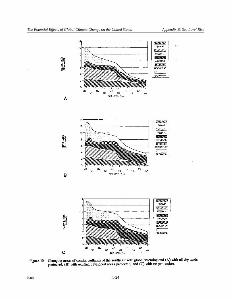
Vegetated wetlands cover 11,73S mi2 in the southeastern states, from North Carolina to Texas; this is 89% of the vegetated wetlands of the contiguous United States. Therefore, the responses of the southeastern wetlands to sea level rise (Figure 10) are similar to those presented for the United States. Coastal responses have been considered separately for several subregions, with examination of sites representing estuarine, deltaic, barrier island, and subtropical carbonate platform environments.

South Atlantic Coastal Plain. This region (Figures 11, 12) is characterized by relatively high tidal ranges and by extensive low terraces representing Pleistocene barrier island systems (such as the sea islands of South Carolina and Georgia). Wetlands are well developed, especially near major rivers where sedimentation and accretion are highest; at present they cover 3,813 mi2 . Because of the high tidal ranges and the availability of lowlands for colonization, these wetlands will be more persistent in the face of rising sea level compared with other U.S. coastal areas (Figure 13). Mangroves can be expected to spread into the more southerly sites if temperatures increase.

Charleston, South Carolina. This historic town is at the confluence of several estuaries with large tidal ranges and extensive marshes. Near the mouth of the harbor Sullivan's Island (celebrated in The Gold Bug by Edgar Allen Poe) forms a barrier island with a well developed back-barrier marsh. The recent rediversion of the Santee River has decreased the high sedimentation that helped promote the historic growth of wetlands; however, assuming no change in historic trends, the model predicts a slight expansion of marshes onto dredge-fill areas by the year 2100 (Figure 14B). With a half-meter rise, most of the saltmarshes would be inundated and converted to tidal flats exposed only at low tide (Figure 14C); increasing sea level stands would lead to widespread inundation.of low-lying areas adjacent to the rivers (Figure 14D-F). The 1-meter scenario yields an estimate of 47% loss of saltmarsh by 2075, which is quite close to the estimate of 51% by 2075 reported by Kana et al. (1988), based on detailed transects.

Sea Island, Georgia . The wetlands of the Georgia Sea Islands have been studied intensively for many years. Marshes are very well developed in the region, due to a combination of high tidal ranges and high sedimentation rates. The site covers two topographic quadrangles, including the communities of Sea Island, St. Simons Island, and part of Brunswick on the mainland (Figure 15). There is no appreciable change in wetlands and adjacent lowlands until almost a 1-meter rise, due to the existence of a 2-meter tidal range (with marshes occupying the upper meter) and a low Pleistocene terrace. With a 1-meter rise and a significantly warmer climate, mangroves would spread onto the low terrace and the marsh would begin to break up. By two meters the community of

Park 1-21


Table 2. Regional and national estimates of losses of coastal marshes and swamps by the year 2100 (in square miles) for the baseline case and four sea4evel scenarios, considering also three levels of shoreline protection: total protection of all dry land, standard protection of areas with residential and commercial development, and no protection. Results are based on simulations using unbiased samples encompassing variable percentages of total area of respective coasts.

Region Sampled Baseline 0.5 m 1 m 2 m 3 m

Northeast 3.36%

Total 88 93 100 188

Standard 39 55 58 33 434

No 27 8 (67) 335

Mid-Atlantic 11.6%

Total 485 520 625 705

Standard (39) 201 341 429 574

No 120 180 361 465

South Atlantic 10.07%

Total 2,295 2,422 2,542 2,736

Standard (59) 1,438 1,669 1,812 2,227

No 1,313 1,516 1,606 2,044

S & W Florida 10.71%

Total 623 829 1,020 1,300

Standard (157) 92 157 165 665

No 63 122 120 631

Louisiana 13.66%

Total 2,450 3,742 4,758 4,801

Standard 2,271 2,368 2,732 4,686 4,776

No 2,345 3,732 4,685 4,778

Other N. Gulf 13.04%

Total 530 1,301 1,121 1,170

Standard 270 396 932 994 1,079

No 360 918 982 1,070

West* 4.87%

Total 37 36 39

Standard (71) (286) (440) (651) (761)

No (332) (518) (791) (843)

United States

Total 6,511 8,673 10,206 10,953

Standard 2,254 4,263 6,441 7,423 8,994

No 3,904 6,046 6,892 8,480

* subject to correction

Park 1-22

53


Park 1-23


Park 1-24


Park 1-25


Park 1-26


Park 1-27


Park 1-28


Park 1-29


Sea Island would either be a diked enclave in the sea or a largely inundated and eroded shoal area. By three meters the only appreciable dry land left, other than in developed areas, would be the Pleistocene beach ridge on Little St. Simons Island.

Southern and Western Coasts of Florida. Southern Florida (Figure 16) is a low-lying carbonate platform and string of coral-reef keys that developed during interglacial epochs when sea level was higher than it is today. A slight rise in sea level, Would inundate this area again. The Everglades are maintained as a broad freshwater marsh by runoff from the interior; the saltwater wetlands are dominated by mangrove swamps which occur over a narrow elevational range due to the low tidal range. This initial study estimated the area of vegetated wetlands.

Everglades City, Florida. This site is characterized by mangrove swamps and low beach ridges, with Everglades on the slightly higher ground (Figure 17). As shown by the maps, mangrove swamps would actually increase in area with sea level rise as the low beach ridges are inundated by a 2-meter rise in sea level. With more than a 2-meter rise, the mangroves would gradually decrease in area.

The west coast north of subtropical southern Florida (Figure 18) has a very gradual slope offshore, marshes on the open coast, a low tidal range, and a low terrace along the coast. Consequently, it too is quite vulnerable to sea level rise. Furthermore, with moderating temperatures, the entire region would become subtropical and mangrove swamps would spread north,

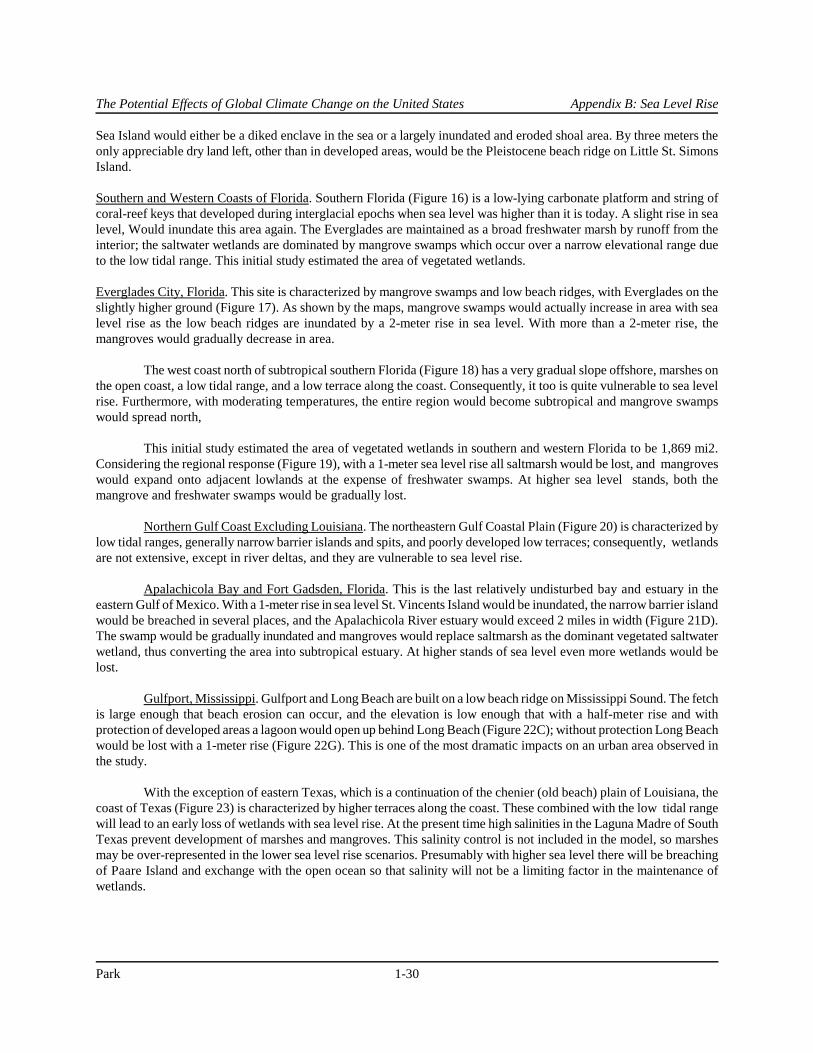
This initial study estimated the area of vegetated wetlands in southern and western Florida to be 1,869 mi2. Considering the regional response (Figure 19), with a 1-meter sea level rise all saltmarsh would be lost, and mangroves would expand onto adjacent lowlands at the expense of freshwater swamps. At higher sea level stands, both the mangrove and freshwater swamps would be gradually lost.

Northern Gulf Coast Excluding Louisiana. The northeastern Gulf Coastal Plain (Figure 20) is characterized by low tidal ranges, generally narrow barrier islands and spits, and poorly developed low terraces; consequently, wetlands are not extensive, except in river deltas, and they are vulnerable to sea level rise.

Apalachicola Bay and Fort Gadsden, Florida. This is the last relatively undisturbed bay and estuary in the eastern Gulf of Mexico. With a 1-meter rise in sea level St. Vincents Island would be inundated, the narrow barrier island would be breached in several places, and the Apalachicola River estuary would exceed 2 miles in width (Figure 21D). The swamp would be gradually inundated and mangroves would replace saltmarsh as the dominant vegetated saltwater wetland, thus converting the area into subtropical estuary. At higher stands of sea level even more wetlands would be lost.

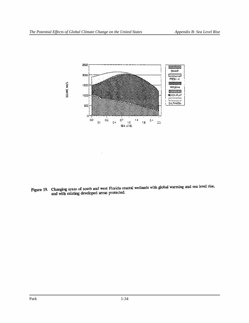
Gulfport, Mississippi. Gulfport and Long Beach are built on a low beach ridge on Mississippi Sound. The fetch is large enough that beach erosion can occur, and the elevation is low enough that with a half-meter rise and with protection of developed areas a lagoon would open up behind Long Beach (Figure 22C); without protection Long Beach would be lost with a 1-meter rise (Figure 22G). This is one of the most dramatic impacts on an urban area observed in the study.

With the exception of eastern Texas, which is a continuation of the chenier (old beach) plain of Louisiana, the coast of Texas (Figure 23) is characterized by higher terraces along the coast. These combined with the low tidal range will lead to an early loss of wetlands with sea level rise. At the present time high salinities in the Laguna Madre of South Texas prevent development of marshes and mangroves. This salinity control is not included in the model, so marshes may be over-represented in the lower sea level rise scenarios. Presumably with higher sea level there will be breaching of Paare Island and exchange with the open ocean so that salinity will not be a limiting factor in the maintenance of wetlands.

Park 1-30


Park 1-31


Park 1-32


Park 1-33


Park 1-34


Park 1-35


Park 1-36


Park 1-37


Park 1-38


Considering the entire northern Gulf Coast other than Louisiana, this study estimates the present area of vegetated wetlands to be 1,218 mi2. A striking pattern of saltmarsh loss would take place, with only a slight rise in sea level (Figure 24); with a one-meter rise most freshwater marshes would be lost as well. With moderating climate saltmarshes would be replaced by mangroves, and the northern Gulf would become a subtropical coastal system.

Louisiana. A surprisingly similar response is predicted for this region (Figure 25). At present vegetated wetlands cover 4,835 mi2. Tidal flats may initially expand as beaches, cheniers (old beaches), and dredge-fill areas are reclaimed by the sea; but saltmarshes will continue their rapid decline; mangroves would increase; and, prior to a 1-meter rise, most freshwater marshes would be lost (Figure 26). The pattern predicted for this region is due to the low tidal range, extensive alluvial and coastal lowlands, high subsidence rates, and high sedimentation rates. Coastal swamps and marshes cover most of the region. Half the wetlands that would be lost in the southeast, with a 1-meter rise in sea level and standard protection of developed areas, are in Louisiana (Table 2).

Luling-Pelican, Louisiana. This strip of four sites forms a transect from the western suburbs of New Orleans (including the airport) to the Gulf of Mexico (Figure 27). The area is now losing wetlands rapidly due to subsidence and human disturbance. The simulations represent an approximate response to sea level rise, but do not represent the complex interactions of changing river courses, floodwater diversions, variable sediment supplies, and salinity controls that affect the coastal ecosystems. These are better treated by region- and site-specific models such as that by Costanza et al. (1987). The tenuous position of the saltmarshes is shown by the baseline simulation in which most of the present saltmarshes are lost by the year 2100 (Figure 27B). The half-meter simulation (Figure 27C) is almost identical to the baseline, which coincides with the flat regional response for that range of sea levels (Figure 26).

West Coast

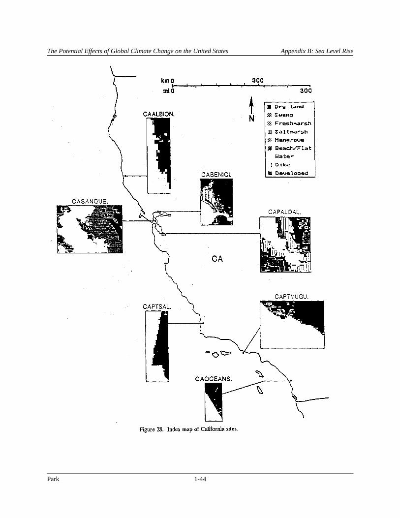
California (Figure 28) is characterized by rugged coastlines with low-lying areas. Most wetlands are in San Francisco Bay, where the high tidal range and high sedimentation rates created extensive wetlands prior to their destruction by dredge fill- and by diking for salt ponds. At present, high subsidence rates and erosion rates are contributing to the decline of the remaining marshes. Heavy development has left little potential for the spread of wetlands onto adjacent lowlands. However, the model shows an unexpected spread of wetlands (Table 2). This appears to be due to -errors in digitizing the elevations; also, salt pannes are not modeled in the current version. Until the data are checked thoroughly, the significant increase in wetlands under all scenarios should be viewed with suspicion.

Benicia, California. The remaining wetlands, now only a fraction of their original extent, are adjacent to developed areas and diked lowlands and salt ponds; they are lost with even a half-meter rise in sea level (Figure 29). If lowland areas were not protected, the marshes would migrate inland with sea level rise.

The Pacific Northwest (Figure 30), like California, is characterized by rugged, high-energy coasts and few low-lying areas. Where the topography is suitable for marsh formation, as in Yaquina Bay, Oregon, high tidal ranges would help to perpetuate those marshes despite a half-meter sea level rise.

Although the sample size is small and the data should be checked further, this initial study estimates the area of current vegetated wetland of the West -Coast to be 64 mi2. As shown in Figure 31 (which illustrates the total protection scenario and is not subject to elevational errors), aggregated wetlands exhibit a rather flat response to sea level rise.

Northeast

This diverse region (Figure 32) is similar to the West Coast with its high tidal ranges and rocky coasts, but includes easily eroded Cape Cod. This initial study estimates the area of vegetated wetlands to be 600 mi2. The subsample of four sites is too small to define the region well; however, a pattern does emerge. Swamps developed on poorly drained glacial tills occur at elevations above those, that could be inundated by sea level rise in the next century and therefore persist. Some coastlines, such as parts of the Maine coast, have no marshes at present and will not develop marshes due to the rocky

Park 1-39


Park 1-40


Park 1-41


Park 1-42


Park 1-43


Park 1-44


Park 1-45


Park 1-46


Park 1-47


Park 1-48


substrate. Other areas have marshes protected by baymouth bars and spits; these marshes will not, be affected adversely by lower stands of sea level.

Watch Hill, Rhode Island. This site includes the historic resort town of that name, with a long, narrow spit maintained by longshore drift to the west. It. also includes. Misquarnicut Beach and adjacent marsh (Figure 33). The marsh will gradually disappear with higher sea level, and eventually Misquamicut Beach will be breached, according to the simulations.

Park 1-49


Park 1-50


CHAPTER 4

SUMMARY

Projections of coastal wetland and lowland changes are made, using, romotely sensed cover-class data; lowland elevations digitized from topographic maps, and a simulation model based on simple geometric relationships of inundation and subsidiary influences of spatially varying exposure and erosion relationships. Approximately 9% of the coast of the contiguous United States was sampled in this phase of 4he study. Forty-six sites were chosen using an unbiased, systematic sample of coastal topographic maps; several additional sites were chosen for purposes of model verification.

Examination of eight representative sites provides, insights into local responses of wetlands to accelerated sea level rise. Some sites, such as Sea Island, Georgia, are well buffered for sea levels up to 1 meter, due to high tidal ranges and high sedimentation and accretion rates. Other sites, especially in the Gulf of Mexico, are quite vulnerable to small changes in sea level; Long Beach, Mississippi, could be completely inundated by less than a 1-meter rise. Although the model is perhaps too simple for representing complex deltaic dynamics, it projects a continuation of current trends for the Louisiana coast south of New Orleans, with the entire undiked area shown to be at risk without- any acceleration in sea level rise.

Composite responses were obtained by summing cover-class areas 4cir ea6h,simulation time step for sites comprising a regional sample, and by transforming the values into regional estimates. The results are presented in Table 2 and as area graphs showing the patterns of changes in wetland areas with an exponential increase in sea level up to 3 meters. Regional responses. are as follows:

• The mid-Atlantic Coast, with 746 mi2 of diverse wetlands and moderate tidal ranges, would probably exhibit a gradual decline in vegetated wetlands and an increase in tidal flits; with standard protection of all currently developed lowlands, 27% of marshes and swamps would be lost with a 0.5-m rise by the year 2100, 46% with a 1-m rise, 58% with a 2-m rise, and 77% with 3-m rise.

• The South Atlantic Coast, with 3,813 mi2 of vegetated wetlands, is predicted to exhibit a gradual decline in vegetated wetlands by the year, 2100, with mangrove swamps replacing saltmarshes as the dominant saltwater vegetated wetland at the more southerly sites; with standard protection, 38% of the fresh- and saltwater wetlands would be lost with a 0.5-m rise, 44% with a 1-m rise, 48% with a 2-m rise, and 58% with a 3-m rise.

• The southern and western coasts of Florida, with 1,869 mi2 of vegetated wetlands, have large expanses of low-lying, undeveloped areas suitable for wetlands to migrate onto; therefore, vegetated wetlands would not decrease greatly in area by 2100 unless extensive dikes were constructed. With standard protection, only 5% of existing vegetated wetlands would be lost with a 0.5-m rise, 8% with a 1-m rise, and 9% with a 2-m rise; however, 36% would be lost with a 3-m rise. As the entire region becomes subtropical, mangrove swamps would spread northward and saltmarshes would gradually disappear.

• The northern Gulf Coast, excluding Louisiana, is estimated to have 1,218 Mi2 of vegetated wetlands; with its low tidal ranges and general lack of suitable lowlands for wetlands to migrate onto, saltmarshes would be lost with low sea-level rises by 2100. With standard protection, 33% of the vegetated wetlands would be lost with a 0.5-m rise, 77% with a 1-m rise, 82% with a 2-m rise, and 89% with a 3-m rise. Mangroves would take the place of saltmarshes as the climate moderates.

• Louisiana is estimated to have had 4,835 mi2 of vegetated wetlands at the time the satellite imagery was obtained; these wetlands are being lost at an alarming rate without accelerated sea-level rise. With standard protection, this study estimates that by 2100, 47% of the vegetated wetlands would be lost with a 0.14-m rise in eustatic sea level (the historic rise continued)i'49% with a 0.5-in rise, 57% with a 1-m rise, 97% with a 2-in

Park 1-51


rise, and 99% with a 3-m rise.

The sample size is too small in this initial study to reach conclusions about the West and Northeast Coasts, but preliminary results suggest that wetlands would be lost gradually due to the ameliorating effect of high tidal ranges.

These regional tabulations were summed to obtain estimates and area graphs for the entire coast of the contiguous United States, which has approximately 14,000 mi2 of coastal wetlands (including 13,145 mi2 of vegetated wetlands) at the present time. With protection of all existing residential and commercial developments, by the year 2100 saltmarshes and freshwater swamps would gradually. decline in area, mangrove swamps would gradually increase, and freshwater marshes would gradually decline until a sea level of 0.8 m is reached. Freshwater marshes would then disappear rapidly (reflecting a pattern seen in both the Gulf. and mid-Atlantic Coasts); 3S% of vegetated wetlands would be lost with a 0.5-m rise, 49% with a 1-m rise, S6% with a 2-m rise, and 68% (almost9.,000 mi2) with a 3-m rise. If all coastal lowlands not already protected by dikes were allowed to be inundated by a 3-m rise, a more gradual loss 6f.saltmarshes would occur compared to the standard protection scenarios; 30% of vegetated wetlands Would be lost with a 0.5-m rise, 46% with a 1-m rise, 52% with a 2-m rise, and 65% with a 3-m rise. Conversely, total protection of all dry land would result in an accelerated decline in saltmarshes and no increase in areas of mangrove swamps; 50% of vegetated wetlands would be lost with a 0.5-m rise, 66% with a 1-m rise, 78% with a 2-m rise,,and 83% with a 3-m rise.

Alternatively, we could consider the sea level rises,of a half meter and 2 meters as being reasonable bounds on a probable 1-meter rise. Therefore, withrio protection of dry land other than existing dikes, 3,900 to 6,900 mi2. of vegetated wetlands could be lost by the year 2100. With existing residential and commercial developments protected, 4,300 to, 714W mi2 of vegetated wetlands could be lost; with all dry land protected, 6,500 to 10,200 mi2 of vegetated wetlands, could be lost.

Wetlands provide important habitat for many fish and wildlife species, including rare and endangered birds on a three coasts, and over half the commercially important coastal fish species of the Southeast. Wetlands also remove pollutants and protect inland areas from floods, storms, and high tides. Therefore, policy decisions should be made to protect these valuable, natural resources from the consequences of global warming and sea level rise.

Park 1-52


REFERENCES

Armentano, T.V., RA. Park, and C.L. Cloonan. 1988. Impacts on wetlands throughout the United States. In Titus, James G. (ed.), Impact of Sea Level Rise on Coastal Wetlands in the United States. Washington: U.S. Environmental Protection Agency, pp. 87-149.

Bahr, L.M., Jr., R. Costanza, J.W. Day, Jr., S.E. Bayley, C. Neill, S.G. Leibowitz, and J. Fruci. 1983. Ecological Characterization of the Mississippi Deltaic Plain Region: A Narrative with Management Recommendations. FWS/OBS-82/69, Slidell, Louisiana: Fish and Wildlife Service, 189 pp.

Barth, M.C., and J.G. Titus. 1984. Greenhouse Effect and Sea Level Rise. New York: Van Nostrand Reinhold.

Bird, E.C.F. 1986. Mangroves and intertidal morphology in Westernport Bay, Victoria, Australia. Marine Geology, 69: 251-271.

Browder, JA., H.A. Bartley, and K.S. Davis. 198S. A probabilistic model of the relationship between marshland-water interface and marsh disintegration. Ecological Modelling 29:245-260.

Bruun, Per. 1962. Sea Level Rise, as a Cause of Shore Erosion. Journal of the Waterways and Harbors Division, Proceedings of the American Society of Civil Engineers, 88(WW1):117-130.

Bruun, Per. 1986. Worldw 'ide Impacts of Sea Level Rise on Shorelines. In Effects of Changes in Stratospheric Ozone and Global Climate, Vol. 4: Sea Level Rise, edited by James G. Titus, 99-128. Washington, DC, U.S. Environmental Protection Agency.

Costanza, R., C. Neill, S.G. Leibowitz, J.R. Fruci, L.M. Bahr, Jr., and J.W. Day, Jr. 1983. Ecological Models of the Mississippi Deltaic Plain Region: Data Collection and Presentation. U.S. Fish and Wildlife Service, Division of Biological Services, Washington, D.C. FWS/OBS-82/68, 342 pp.

Costanza, R., F.H. Sklar, M.L. White, J.W. Day, Jr. 1987. A dynamic spatial simulation model of land loss and marsh succession in coastal Louisiana In: Wetland, Modelling, W.J. Mitsch, M. Strasraba, and S.E. Jorgensen (eds.,), Elsevier, Amsterdam.

Dasarathy, B.V. 1974, HINDU: Histogrwn Inspired Neighborhood Discerning Unsupervised Pattern Recognition System. NASA/Computer Sciences Corp., Huntsville, Alabama, 43 pp.

Davis, RA. 1985. Coastal Sedimentary Environments. New York: Springer-Verlag.

Day, J.W., Jr. W.G. Smith, P.R. Wagner, and W.C. Stowe. 1973. Community Structure and Carbon Budget of a Salt Marsh and Shallow Bay Estuarine System in Louisiana. Center for Wetland Resources, Louisiana State University, Baton Rouge. Publ. No. LSU-SG-72-04.

Dyer, K.R. 1986. Coastal and Estuarine Sediment Dynamics. Chichester, UK: John Wiley & Sons, 342 pp.

Estes, JA., and GA. Thorley. 1983. Manual of Remote Sensing. Vol. 11: Interpretations and Applications. Second Edition. American Society of Photogrammetry.

Gosselink, J.G. 1994. The Ecology of Delta Marshes of Coastal Louisiana: A Community Profile. FWS/OBS-84/09, Washington, DO U.S. Fish and Wildlife Service, 134 pp.

Hall, S.L., W.R. Wilder, and F.M. Fisher. 1986. An analysis of shoreline erosion along the northern coast of East

Park 1-53


Galveston Bay, Texas. Journal of Coastal Research 2:173-179.

Kana, T.W., BJ. Baca, and M.L. Williams. 1988a. Charleston case study. In: J. G. Titus (ed.), Greenhouse Effect, Sea Level Rise and Coastal Wetlands. EPA-230-05-86-013, U.S. Environmental Protection Agency, Washington, pp. 37-59.

Kana, T.W., W.C. Eiser, B J. Baca, and M.L. Williams. 1988b.- New Jersey case study. 1w. J. G. Titus (ed.), Greenhouse Effect, Sea Level Rise and Coastal Wetlands. EPA-230-05-86-013, U.S. Environmental Protection Agency, Washington, pp. 61-86.

Leatherman, S.P. and R.E. Zaremba. 1986. Dynamics of a northern barrier beach: Nauset Spit, Cape Cod, Massachusetts. Geological Society of America Bulletin. 97:116-124.

Lefor, M.M., W.C. Kennard, and D.L. Civco. 1987. Relationships of salt-marsh plant distributions to tidal levels in Connecticut, USA. Environmental Management 11:61-68.

Letzsch, W.S. and R.W. Frey. 1980. Deposition and Erosion in a Holocene Salt Marsh, Sapelo Island, Georgia. Journal of Sedimentary Petrology, 50(2):529-S42.

Lugo, A.E., and M.M. Brinson. 1978. Calculations of the value of salt water wetlands. In Wetland Functions and Values: The State of Our Understanding, pp. 120-130, American Water Resources Association.

Mausel, P.W. 1985., Remote Sensing: Introduction to Computer Assisted Techniques. ISURSL Information Note 09031985. Indiana State University Remote Sensing Lab, Terre Haute, pp. 72-79.

Montague, C.L., AN. Zale, and H.F., Percival. 1987. Ecological effects of coastal marsh impoundments: a review. Environmental Management, vol. 11, pp. 743-756.

Park, R.A., T.V. Armentano, and C.L. Cloonan. 1986a. Predicting the impact of sea level rise on coastal systems. In Supplementary Proceedings for the 1986 Eastern Simulation Conference, Norfolk, Virginia, pp. 149-153.

Park, R.A., T.V. Armentano, C.L. Cloonan. 1986b. Predicting the effects of sea level rise on coastal wetlands. In James G. Titus (ed.), Effects of Changes in Stratospheric Ozone and Global Climate, Vol. 4: Sea Level Rise, pp. 129-152, Washington: U.S. Environmental Protection Agency.

Peltier, W.R. 1988. Global sea level and earth rotation. Science, vol. 240, pp. 895-901.

Pope, R.M., and J.G. Gosselink. 1973. A tool for use in making land management decisions involving tidal marshland. Coastal Zone Management Journal. 1:65-74.

Ryszkowski, Lech. 1984. Primary production in agroecosystems. Options Mediterraneennes. Mediterranean Agronomic Institute of Saragossa, Spain, 84(l):77-94.

Sherrod, C.L., and C. McMillan. 1985. The distributional history and ecology of mangrove vegetation along the northern Gulf of Mexico. Contributions in Marine Science, 28:129-140.

Sklar, R. Costanza, and J. W. Day, Jr. 1985. Dynamic spatial simulation modeling of coastal wetland habitat succession. Ecological Modelling 29:261-281.

Swanson, R.L., and C.I. Thurlow. 1973. Recent subsidence rates along the Texas and Louisiana coasts as determined from tide measurements. Journal Geophysical Research 78:2665-2671.

Teal, J.M. 1962. Energy flow in the salt marsh ecosystem of Georgia. Ecology. 43:614-624.

Park 1-54


Teal, J.M., and M. Teal. 1969. Life and Death of the Salt. Marsh. New York: Audobon-Ballantine.

Thomas, R. 1986. Future sea level rise and its early detection by satellite remote sensing. In James G. Titus (ed.), Effects of Changes in Stratospheric Ozone and Global Climate, Vol. 4: Sea Level Rise pp. 19-36, Washington: U.S. Environmental Protection Agency.

Thurman, H.V. 1983. Essentials of Oceanography. Columbus, Ohio: Charles E. Merrill.

Titus, J.G. ed. 1986. Effects of Changes in Stratospheric Ozone and Global Climate, 4 vols. Washington: U.S. Environmental Protection Agency.

Titus, J.G. ed. 1988. Greenhouse Effect, Sea Level Rise and Coastal Wetlands. EPA-230-05-86-013, Washington: U.S. Environmental Protection Agency.

Titus, J.G., and S.R. Seidel. 1986. Overview of the effects of changing the atmosphere. In James G. Titus (ed.), Effects of Changes in Stratospheric Ozone and Global Climate, Vol. 1: Overview, pp. 3-19, Washington: U.S. Environmental Protection Agency.

Villach. 1985. International assessment of the role of carbon dioxide and of other greenhouse gases in climate variations and associated impacts. Conference Statement. Geneva: United Nations Environment Program.

Watkins, J.S., M.L. Bottino, and M. Morisawa. 1975. Our Geological Environment. Philadelphia: W. B. Saunders.

Wiegert, R.G., R.R. Christian, J.L. Gallagher, J.R. Hall, R.D.H. Jones, and R.L. Wetzel. 1975. A preliminary ecosystem model of a coastal Georgia Spartin marsh. In Estuarine Research, Vol. 1, edited by L. E. Cronin, pp. 583-601. New York: Academic Press.

Park 1-55


Park 1-56

The Effects of Sea Level Rise on U.S. Coastal...

Documents

Transcript of The Effects of Sea Level Rise on U.S. Coastal...