
The effects of Jonglei Canal operation scenarios on the Sudd
64
The effects of Jonglei Canal operation scenarios on the Sudd swamps in Southern Sudan Twente University Erwin Lamberts August, 2009
Transcript of The effects of Jonglei Canal operation scenarios on the Sudd
TThhee eeffffeeccttss ooff JJoonngglleeii CCaannaall ooppeerraattiioonn
sscceennaarriiooss oonn tthhee SSuudddd sswwaammppss iinn SSoouutthheerrnn
SSuuddaann
Twente University
Erwin Lamberts
August, 2009

The effects of Jonglei Canal operation scenarios on the Sudd swamps in Southern Sudan 2
The effects of Jonglei Canal operation scenarios on the Sudd swamps in Southern Sudan 3
Preface
In front you will find my master thesis about the effects of the implementation of
Jonglei Canal scenarios on the Sudd swamps in Southern Sudan. This thesis is made as
the completion of the master study Civil Technology & Management at the Twente
University.
During my education I got more and more interested in the water management part
of my study. Especially the hydrology side of this part got my interest. When I needed
to find an assignment for my master thesis, my eye fell on the Nile catchment with it
complex hydrology of the Sudd area. A chance I couldn’t resist.
First of all I would like to thank my advisor from Deltares, prof. ir. E. (Eelco) van Beek.
He gave me the opportunity to start with my master study in Delft. Although I couldn’t
finish my master thesis there due to some health problems, I had a great experience
being there and had a good work social environment and nice colleagues. My
advisor at the UT, dr. M.S. (Maarten) Krol, I would like to thank for his detailed
feedback and his support during my graduation process. At last, I would to thank PhD
Y.A. (Yasir) Mohamed, for his help and ideas for my master thesis due to his great
knowledge about the area.
Erwin Lamberts

The effects of Jonglei Canal operation scenarios on the Sudd swamps in Southern Sudan 4
Summary
The Sudd, one of the largest wetland areas in the world, is faced by huge
evapotranspiration rates. More than 50 % of the Sudd inflow is evaporated out of the
Sudd swamps, resulting in less water availability in the downstream areas. To gain
extra water downstream, planners have proposed to dig a canal (Jonglei canal)
around to Sudd area, to save an extra 4.8 Gm3/year. What the effects of the swamps
in the Sudd area will be, are still relatively unknown. In this thesis the effects on the
Sudd swamp will be studied based on several Jonglei Canal scenarios.
In the first phase of the study the historical monthly water balance for the period 1961
– 2000 has been simulated. This is done by creating a hydrological model based on
the water balance made by Sutcliffe & Parks (1987). This model describes the Sudd as
a reservoir, where the input comes from the precipitation and the inflow, and the
output from the evapotranspiration and the outflow.
To simulate the water balance, several data sets had to be collected. The first data
set is the precipitation data in the Sudd area. This data was collected at the Global
Precipitation Climatology Centre (GPCC). The next data set is the evapotranspiration
data. This data was simulated with the use of the ET0 calculator (FAO, 2009). The ET0
calculator uses the Penman-Monteith equation for the calculation of the
evapotranspiration. The input for the calculator is collected at the measurement
stations at Juba and Malakal for the temperature, relative humidity and the sunshine
hours. The inflow data set is collected at the measurement stations Mongalla
simulated in the RIBASIM model. The RIBASIM model simulates the monthly water flows
for several measurement stations in the Nile basin. The outflow for the Sudd is based
on the flows at the stations Malakal and Doleib Hill. The outflow is described as the
flow of Malakal minus the flow at Doleib Hill. The data for the period 1961 – 1983 has
been measured and the data for the period 1983 – 2000 will be simulated by a
regression equation between the flows at Malakal and Doleib Hill.
When all the data sets were collected, the historical water balance for the Sudd
could be simulated. The results from the water balance show that the swamp sizes in
the period 1961 – 1964 increased by almost 300 % from 15 Gm2 to around 60 Gm2. In
the period 1965 – 1978 the swamp sizes recovers to around 42 Gm3 where it slightly
decreased to 35 Gm2 until 1978. In the period 1979 – 1981 the swamps show a sudden
size increase. This is caused by a high increase in the precipitation in that period. In
the last period until 2000 the Sudd swamps fluctuates around 30 Gm2.
The second phase of the study several Jonglei canal scenarios have been tested. The
scenarios are placed in three groups: fixed canal flows, seasonal dependent canal
flows and flows where the extra water volume downstream of the Sudd will be 4.8
Gm3/year. For the simulation of the swamps with the canal flows some variables
needed to be adjusted. The inflow will now be decreased by the flow through the
canal. The evapotranspiration will change under influence from a changing relative
humidity as a result of the drained area. At last the outflow will change. The Sudd
outflow is linear related to the swamp area where there will be a division in a dry
period relation and a wet period relation.
The results from the fixed canal flows show a high linear relation between the flows
and the change in the permanent (16 – 26 %), seasonal (13 – 22 %) and total swamp
(15 – 25 %). The effects on the permanent swamp will be the highest, followed by the
total swamp and at last the seasonal swamp.
The effects with seasonal dependent canal flows will be the highest on the size of
seasonal swamp. The change on the permanent swamp depends mainly on the total

The effects of Jonglei Canal operation scenarios on the Sudd swamps in Southern Sudan 5
yearly flow. When this total is high, the decrease of the permanent swamp will also be
high. The change on the seasonal swamp depends on the size of the canal flow in
the wet period. When this is high, the decrease of the seasonal swamp will also be
high. The change on the total swamp depends, just like the permanent swamp, on
the total yearly flow.
To create 4.8 Gm3/year water downstream of the Sudd, the average canal flow need
to be 18 Mm3/day. The scenario, a canal flow of 10 Mm3/day in the dry period and 26
Mm3/day in the wet period, has the highest influence on the total swamp, almost
26 %. The same scenario has the highest influence on the seasonal swamp. The
scenario, a canal flow of 26 Mm3/day in the dry period and 10 Mm3/day in the wet
period, has the highest influence on the permanent swamp, although the difference
between the scenarios is small.

The effects of Jonglei Canal operation scenarios on the Sudd swamps in Southern Sudan 6
Table of contents
Introduction .................................................................................................................................... 8 1.1 General ........................................................................................................................... 8 1.2 Historical studies ............................................................................................................ 9 1.3 Problem analysis.......................................................................................................... 10 1.4 Research objective .................................................................................................... 11 1.5 Research question and criteria ................................................................................ 11 1.5 Approach of the study .............................................................................................. 12
2. Description of the Sudd wetland .................................................................................... 14 2.1 General ......................................................................................................................... 14 2.2 Visualization ................................................................................................................. 14 2.3 Climate ......................................................................................................................... 15 2.4 Hydrological background ......................................................................................... 16 2.5 Flora and fauna .......................................................................................................... 17
3. Hydrological model ........................................................................................................... 18 3.1 General ......................................................................................................................... 18 3.2 The model .................................................................................................................... 18 3.3 Adaptation of the hydrological model with Jonglei Canal flows ..................... 22 3.4 Implementation of the hydrological model .......................................................... 22
4. Precipitation ........................................................................................................................ 23 4.1 General ......................................................................................................................... 23 4.2 Data .............................................................................................................................. 23 4.3 Output ........................................................................................................................... 24
5. Evapotranspiration ............................................................................................................. 26 5.1 Evaporation, transpiration and evapotranspiration ............................................ 26 5.2 Reference evapotranspiration (ET0) ........................................................................ 26 5.3 FAO Penman-Monteith equation ............................................................................ 27 5.4 Calculation of ET0 ........................................................................................................ 28 5.5 From reference evapotranspiration to actual evapotranspiration .................. 28 5.6 Results ............................................................................................................................ 29
6. Inflow ..................................................................................................................................... 31 6.1 General ......................................................................................................................... 31 6.2 Data .............................................................................................................................. 32 6.3 Output ........................................................................................................................... 32
7. Outflow ................................................................................................................................. 35 7.1 General ......................................................................................................................... 35 7.2 Data .............................................................................................................................. 35 7.3 Output ........................................................................................................................... 37
8. The water balance ............................................................................................................ 39 8.1 Simulation of the historic Sudd water balance ..................................................... 39 8.2 Verification of the Sudd water balance ................................................................ 41 8.3 Conclusions on the simulation of the historic water balance ............................ 42
9. The operation of the Jonglei canal ................................................................................ 44 9.1 General ......................................................................................................................... 44 9.2 The effects .................................................................................................................... 44 9.3 Operation rules of the Jonglei Canal ..................................................................... 45 9.4 Adjustments in the hydrological model ................................................................. 45 9.5 Set of scenarios I: Fixed canal flows ........................................................................ 48 9.6 Set of scenarios II: Seasonal dependent canal flows .......................................... 50 9.7 Set of scenarios III: Extra 4.8 Gm3/year water downstream of the Sudd ......... 53 9.8 Conclusions on the operating scenarios of the Jonglei Canal ......................... 54
10. Discussions & Recommendations ................................................................................ 56 10.1 Discussions .................................................................................................................... 56 10.2 Recommendations ..................................................................................................... 57
References .................................................................................................................................... 58

The effects of Jonglei Canal operation scenarios on the Sudd swamps in Southern Sudan 7
Appendix....................................................................................................................................... 60 Appendix A Calculation of ET0 ............................................................................................. 60

The effects of Jonglei Canal operation scenarios on the Sudd swamps in Southern Sudan 8
Introduction
1.1 General
The Sudd wetland is one of the largest wetland areas worldwide and is located along
the Nile in southern Sudan between Mongalla in the south and Malakal in the north,
covering an area of 500 km (north – south) and 200 km (east – west) (see Figure 1).
The size of the wetland is variable, consisting of permanent swamps during the dry
season (November until March) and seasonal swamps, created by flooding of the
Nile (Bahr el Jebel), in the wet season (April until October). On average over the last
50 years the total swamp size consists 60 % of permanent swamps and 40 % of
seasonal swamps (Sutcliffe & Parks, 1987). The annual pattern of flooding is an
essential feature for the ecosystem of the area and is considered crucial to the local
flora and fauna and to the way of life of the local people. T
Figure 1 The Sudd area within the Nile catchment
The effects of Jonglei Canal operation scenarios on the Sudd swamps in Southern Sudan 9
The seasonal river flooded lands (toichs) are a yearly dynamic phenomenon caused
by seasonality in the discharge of the Bahr el Jebel and the geomorphology of the
area. The toichs are a vital component of the grazing cycle for the cattle and wildlife
in particular the dry season. The permanent swamps, flooded throughout the year,
are less economically valuable, though it is a refuge to wildlife. Wildlife migrates from
high land during the rainy season to rain-flooded grasslands at the end of the rains.
For the local people the livestock is an important part of the economy, and there is
no alternative to the toichs in a grazing economy without recourse to irrigated
grassland.
The Sudd wetland is characterized by huge evaporation which results in a lower
water availability for the downstream areas. The evaporation from the Sudd is
estimated to be more than 50 % of the Nile inflow into the Sudd near Mongalla, i.e.
about 28 Gm3/yr out of the 49 Gm3/yr during the period 1961-1983.
To save extra water for use downstream the Sudd, hydrologists in the early part of the
20th century proposed digging a canal, the Jonglei Canal, east of the Sudd which
would divert water from a point below Bor, to a point on the Sobat River, just above
its confluence with the White Nile. The canal was planned to be 360 km long, 50 m
wide and 4 m deep and will divert about 20 million m3 of water per day around the
swamps and will save about an extra 4.8 Gm3/yr which is distributed equally between
Sudan and Egypt. The canal will be navigable and will be constructed beside an all
weather road, both of which will improve communications in the area. However, it is
clear that the canal will bring about a diminution of the Sudd and a change in the
distribution of the wetlands in the area.
The decision to construct the canal was made in 1974 by the Permanent Joint
Technical Commission for Nile Waters (PJTC). The construction began in 1978, but the
political instability in Sudan held up work after 1983. Until this day only 260 km of the
total 360 km have been excavated. Several studies have been carried out to
estimate the effects on the Sudd area when the Jonglei Canal would be completed,
but until this day there aren´t many firm conclusions about the impact on the Sudd
swamp.
1.2 Historical studies
Literature from different authors has been reviewed to obtain a picture on available
information on the Sudd swamps. First comprehensive assessments of the Sudd
hydrology are available from Hurst & Philips (1938) and Butcher (1938). Both authors
described meteorological conditions, topography, hydrology and vegetation in the
swamps and investigated the losses of half the inflowing waters which evaporated in
the swamps.
In 1948, Penman assessed and established general methods to estimate evaporation
in wetland areas. Detailed studies regarding this topic in the Sudd swamp were
carried out by Migahid in 1948 and 1952, aiming at improving the understanding of
the swamp vegetation and related evaporation losses.
With plans for the Jonglei Canal being brought forward, extensive assessments were
carried out to investigate the Sudd, mainly focusing on the area between Mongalla
and Bor. The Jonglei Investigation Team (JIT, 1954) carried out surveys providing a
comprehensive account of the situation in the swamps, describing its topography,
ecology, hydrology, inhabitants, agriculture and fisheries as well as the potential
impacts of the planned canal scheme. Sutcliffe who was part of the investigation
team extended this work, providing a detailed picture of the Sudd topography south

The effects of Jonglei Canal operation scenarios on the Sudd swamps in Southern Sudan 10
of Bor and describing the flow, spill and flooding conditions in this area as well as
ecological factors and the flood cycle dependency of the local economy. In various
papers Sutcliffe provided further details of the southern Sudd hydrology (Sutcliffe,
1974) describing the flood process as flow along a series of basins down the
floodplain. Sutcliffe & Parks (1987) further expanded the description of hydrological
processes in the Sudd by establishing a mathematical model which was used to rout
river flows and assess flood extents under different flow conditions based on water
balance equations utilizing precipitation and evapotranspiration in combination with
inflow and outflow data at Mongalla and Malakal respectively. River Sobat flow data
as recorded at Doleib were subtracted from the Malakal flows in order to take them
out of the equation, Bahr el Ghazal flows were considered to be of negligible
influence. This model was further used to assess the effects of the by then stopped
Jonglei Canal scheme on the flood extent under different flow conditions. Similar
studies have been conducted by Mefit-Babtie (1983) and Howell et al. (1988).
As described above, the latest study that used a mathematical model to calculate
the Sudd water balance was made in 1987 by Sutcliffe & Parks. Since that date there
has been better knowledge and data (like remote sensing techniques), especially
about the evatranspiration losses in the Sudd (Mohamed, 2005). Next, the water
balance of the Sudd was represented in a model of the entire Nile basin, used for
policy analysis at basin level (Ribasim, 2009); this model however was not applied in
particular to assess effects on the Sudd. With this increased knowledge and with the
availability of new data, there lies an opportunity to get a more accurate view of the
water balance in the Sudd and the change in Sudd swamps.
In this study there will be made a monthly calculation of the water balance for the
period 1961 – 2000 with the use of the existing hydrological model for the Sudd,
created by Sutcliffe & Parks. The difference in this new calculation compared to
Sutcliffe and Parks will be the extension of the water balance until 2000, the use of
actual evapotranspiration instead of open water evaporation, and more accurate
data for the precipitation in the Sudd area.
1.3 Problem analysis
The Nile discharges its water into the Sudd wetlands, a network of lakes, channels and
swamps, which are characterized by high evaporation rates that have huge effects
of the water availability in the areas direct downstream. The increased water
demands of these areas, for particularly irrigation projects, forced planners to search
for additional water flows by building short cut channels to bypass the Sudd wetland
(e.g. the unfinished Jonglei Canal).
The Jonglei Canal should create positive effects in the downstream part of the Nile
basin, but can create certain problems for people and flora and fauna in the Sudd
area. The diversion of the water may most likely cause the Sudd swamps and
associated floodplains to shrink which can give the following effects on the area:
I. The annual process of seasonal inundation from river flooded grasslands
(toichs) produces species of grasses, that sustain the livestock and the wild life
during the driest months of the year, can be interrupted (effect on seasonal
swamp).
II. A severe decrease in the discharge into the Sudd would cause the
disappearance of many lakes in the papyrus zone which causes a serious loss
of fishing in the area (effect on permanent swamp).
III. The annual floods are crucial to the maintenance of biological diversity and
the ecosystem in the Sudd (effect on total swamp).
The effects of Jonglei Canal operation scenarios on the Sudd swamps in Southern Sudan 11
1.4 Research objective
The goal of this study is to analyze different operating rules of the Jonglei Canal with
the use of a hydrological model to enhance water supply towards downstream while
minimizing the effects on the change of the size and seasonal cycle of the Sudd.
Operating the Jonglei Canal gives the opportunity to influence the dynamics of the
Sudd area during the year by regulating the discharge through the canal.
1.5 Research question and criteria
The main research question of this study is how the Jonglei Canal can be regulated to
minimize the above described effects of the implementation of the canal while
increasing downstream water availability with a fixed amount. To answer this research
question, several operating rules of the canal will be investigated.
The criteria for the most suitable operating rule will be as follow, where the Jonglei
operating situation will be compared with the normal (no Jonglei Canal) situation:
1. What is the effect on the total, permanent and seasonal swamp size (Δkm2)?
2. Will there be a change in the relation permanent/seasonal swamp size (Δ%)?
3. What will be the effect on the flows downstream the Sudd area (Δm3)?

The effects of Jonglei Canal operation scenarios on the Sudd swamps in Southern Sudan 12
1.5 Approach of the study
The goal of this study is to get insight in the results from different Jonglei Canal
scenarios on the change of the swamp size in the Sudd. To achieve this goal, the
steps in figure 2 will be followed. In the diagram, the steps are numbered that need to
be made to come to the final goal. The process is divided into seven steps:
The process
Calculation of
the water
balance and
swamp sizes
Verification of
the water
balance
Calculation of the water
balance for different
scenarios of the Jonglei
Canal
Creating
hydraulical
model
Evapotranspiration
Precipitation
Outflow
Inflow
Scnarios Jonglei
canal
Evaluating results with
goals and criteria
1
2
3
4
5
6
7
Steps
Flow dataClimate data
Figure 2 The different steps that will be made during this study

The effects of Jonglei Canal operation scenarios on the Sudd swamps in Southern Sudan 13
The description of the 7 steps:
1 Creating the model, based on the hydrological model of Sutcliffe & Parks
(chapter 3)
2 The collection of the monthly data in the Sudd area for the inflow, outflow,
precipitation and evapotranspiration for the period 1961 – 2000 (chapter
4,5,6 and 7)
3 The monthly water balance will be simulated using the hydrological model for
the water balance (chapter 8.1)
4 The simulated water balance c.q. swamp sizes will be verified with existing
measured swamp sizes from satellite assessments (chapter 8.2)
5 Different scenarios for the Jonglei Canal will be created (chapter 9.3)
6 The created scenarios will be simulated (chapter 9.4, 9.5 and 9.6)
7 The results from the different Jonglei Canal scenarios will be compared to the
goals and criteria (chapter 9.7)
With the completion of these steps the goal of the study will be achieved.

The effects of Jonglei Canal operation scenarios on the Sudd swamps in Southern Sudan 14
2. Description of the Sudd wetland
2.1 General
The Sudd wetland is one of the largest wetlands in the world and is located between
4,5° to 9,5°N and 29,5° to 31,5° E (Figure 1). The exact boundaries of the swamp are
difficult to specify, because of its immense dimensions and inaccessibility of the area.
Attempts to define its size are based on hydrological models, on remote sensing, or
on both. The average area of the Sudd wetland is estimated between 30,000 and
40,000 km2 (Sutcliffe & Parks, 1987). The wetland of the Sudd is composed of
interconnected (sometimes parallel) river channels, associated with huge flood
plains. The permanent swamps, usually close to the main river courses are
permanently wet. However, substantial parts of the Sudd are seasonal swamps
created by flooding of the Nile or when ponds are filled seasonally with rainwater
(Howell et al., 1988).
2.2 Visualization
The permanent swamps of the Sudd begin at Mongalla where they are 10-13 km
wide over a straight line distance of 115 km, until Bor. After Bor the swamps widen up
to 25 km and with the peripheral floodplains even wider. Major channels occur to the
east, and there are several large lakes enclosed by permanent swamps on both
banks. At Zeraf Cuts two canals on the east bank join the main channel of the Bahr el
Jebel with the Bahr el Zeraf, but only the southern canal is kept open. Here, water
flows from the Bahr el Jebel to the Bahr el Zeraf, which reenters the Bahr el Jebel near
Tonga and thus isolates Zeraf Island between the two rivers. This island, east of the
Bahr el Jebel, 180 km long and up to 65 km wide, was once mostly dry land, but
following the rise in water levels after the 1960s, it has become a seasonal floodplain.
Meanwhile the seasonal floodplain on the west bank of the Bahr el Jebel is 25 km
wide in places and at Lake No, 190 km due north of Zeraf Cuts, the Bahr el Jebel
receives the Bahr el Ghazal. From Lake No, the river, now often known as the White
Nile, swings abruptly eastwards for 115 km to a confluence with the Sobat River. It
then flows northeastwards, past Malakal, having left the Sudd above the Sobat.
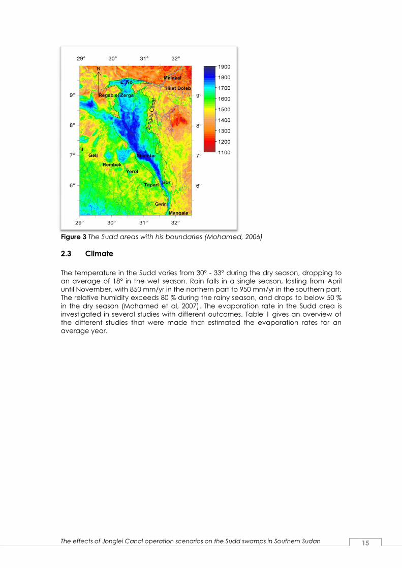
The evaporation map in figure 3 gives an estimation of the extension of the Sudd
wetland, with the dark blue parts as the permanent swamp and the light blue/green
parts the seasonal swamps.
The effects of Jonglei Canal operation scenarios on the Sudd swamps in Southern Sudan 15
Figure 3 The Sudd areas with his boundaries (Mohamed, 2006)
2.3 Climate
The temperature in the Sudd varies from 30° - 33° during the dry season, dropping to
an average of 18° in the wet season. Rain falls in a single season, lasting from April
until November, with 850 mm/yr in the northern part to 950 mm/yr in the southern part.
The relative humidity exceeds 80 % during the rainy season, and drops to below 50 %
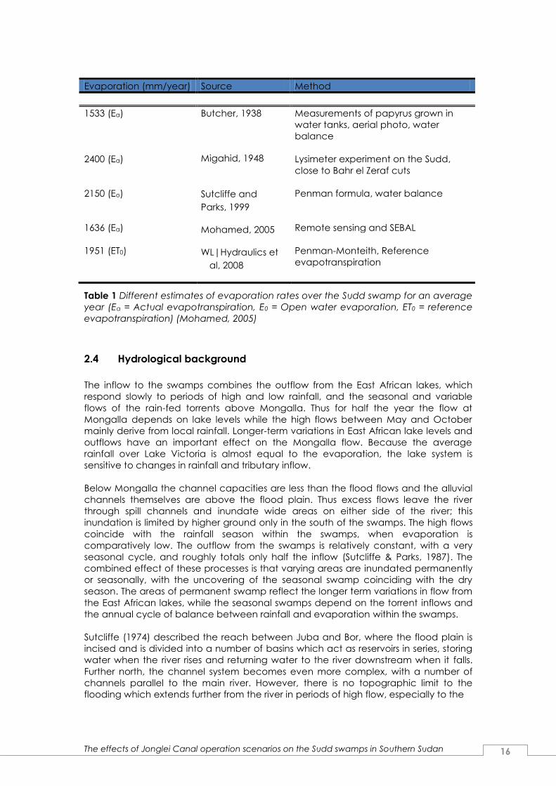
in the dry season (Mohamed et al, 2007). The evaporation rate in the Sudd area is
investigated in several studies with different outcomes. Table 1 gives an overview of
the different studies that were made that estimated the evaporation rates for an
average year.
The effects of Jonglei Canal operation scenarios on the Sudd swamps in Southern Sudan 16
Evaporation (mm/year) Source Method
1533 (Ea)
2400 (Ea)
2150 (Eo)
1636 (Ea)
1951 (ET0)
Butcher, 1938
Migahid, 1948
Sutcliffe and
Parks, 1999
Mohamed, 2005
WL|Hydraulics et
al, 2008
Measurements of papyrus grown in
water tanks, aerial photo, water
balance
Lysimeter experiment on the Sudd,
close to Bahr el Zeraf cuts
Penman formula, water balance
Remote sensing and SEBAL
Penman-Monteith, Reference
evapotranspiration
Table 1 Different estimates of evaporation rates over the Sudd swamp for an average
year (Ea = Actual evapotranspiration, E0 = Open water evaporation, ET0 = reference
evapotranspiration) (Mohamed, 2005)
2.4 Hydrological background
The inflow to the swamps combines the outflow from the East African lakes, which
respond slowly to periods of high and low rainfall, and the seasonal and variable
flows of the rain-fed torrents above Mongalla. Thus for half the year the flow at
Mongalla depends on lake levels while the high flows between May and October
mainly derive from local rainfall. Longer-term variations in East African lake levels and
outflows have an important effect on the Mongalla flow. Because the average
rainfall over Lake Victoria is almost equal to the evaporation, the lake system is
sensitive to changes in rainfall and tributary inflow.
Below Mongalla the channel capacities are less than the flood flows and the alluvial
channels themselves are above the flood plain. Thus excess flows leave the river
through spill channels and inundate wide areas on either side of the river; this
inundation is limited by higher ground only in the south of the swamps. The high flows
coincide with the rainfall season within the swamps, when evaporation is
comparatively low. The outflow from the swamps is relatively constant, with a very
seasonal cycle, and roughly totals only half the inflow (Sutcliffe & Parks, 1987). The
combined effect of these processes is that varying areas are inundated permanently
or seasonally, with the uncovering of the seasonal swamp coinciding with the dry
season. The areas of permanent swamp reflect the longer term variations in flow from
the East African lakes, while the seasonal swamps depend on the torrent inflows and
the annual cycle of balance between rainfall and evaporation within the swamps.
Sutcliffe (1974) described the reach between Juba and Bor, where the flood plain is
incised and is divided into a number of basins which act as reservoirs in series, storing
water when the river rises and returning water to the river downstream when it falls.
Further north, the channel system becomes even more complex, with a number of
channels parallel to the main river. However, there is no topographic limit to the
flooding which extends further from the river in periods of high flow, especially to the

The effects of Jonglei Canal operation scenarios on the Sudd swamps in Southern Sudan 17
Northeast where there is a lack of defined channels and it is doubtful whether much
of the spill returns to the main river. The flooding pattern is complex but may be
described by a water balance model, where the swamp storage is represented by a
reservoir.
2.5 Flora and fauna
The Sudd is one of the largest floodplains in Africa, providing watering and feeding
grounds for populations of migratory mammals and birds. This floodplain borders the
arid Sahelian region and is an important watering place for many species as they
move across the landscape. The floodplain ecosystem supports a variety of plant
species. Wild rice grassland dominates the seasonally inundated floodplains. This
seems to suggest that rice may grow in the Sudd area. Improved rice varieties may
grow in the floodplains in addressing poverty in Southern Sudan. During the 1980s
Southern Sudan had among the highest population levels of antelope in Africa and
the Sudd has been listed as a key location for the recovery of threatened antelope in
Sub-Saharan Africa. Among the most abundant species found are the white-eared
kob, the tiang and the Mongalla gazelle and these three species of antelopes make
large-scale migration over the relatively undisturbed habitat of the Sudd. A million
individuals of white-eared kob undertake a massive migration following the
availability of floodplain grasses.
It is to be noted that the floodplains of the Sudd provide important habitat for several
species of birds. The floodplains support the largest population of shoebill in Africa.
The endangered white pelican flies over 2,000 kilometers from Eastern Europe and
Asia to reach one of its most important wintering grounds on the floodplains of the
Sudd. The Sudd is also a stronghold for the black crowned cranes, a species that has
been designated vulnerable. Annual floods are crucial to the maintenance of
biological diversity in the Sudd. The Dinka, Nuer and Shilluk (or Cholo) co-exist in the
Sudd with tens of thousands of large herbivores depend on the annual floods and
rain to regenerate floodplain grasses which feed their herds of cattle. Fishing in the
Sudd is also a means of livelihood. (Howell et al, 1988)
The completion of the Jonglei canal project is likely to affect the bio diversity and
ecosystem of the Sudd area as a result of the decreased water availability. At any
rate it is seen that diversion of the water may most likely cause the Sudd swamps and
associated floodplains to shrink dramatically, threatening the fauna and flora that
depend on the swamps and floodplains for survival.
The Jonglei canal is also likely to have a significant impact on climate, groundwater
recharges, silt and water quality. This involves the loss of fish habitat and grazing areas
which in turn will have serious implications for the people of the area.
The seasonal river flooded lands (toichs) are a yearly dynamic phenomenon caused
by the extreme variable rainfall in the area. The toichs are a vital component of the
grazing cycle for the cattle and wildlife in particular the dry season (Howell et al,
1988). The permanent swamps, flooded throughout the year, are less economically
valuable, though it is a refuge to wildlife. Wildlife migrates from high land during the
rainy season to rain-flooded grasslands at the end of the rains. For the local people
the livestock is an important part of the economy, and there is no alternative to the
toichs in a grazing economy without recourse to irrigated grassland. It may be clear
that the toichs are crucial to the economy at this time of year. It is however, just these
grasslands that may be reduced by the operation of the canal.
The effects of Jonglei Canal operation scenarios on the Sudd swamps in Southern Sudan 18
3. Hydrological model
3.1 General
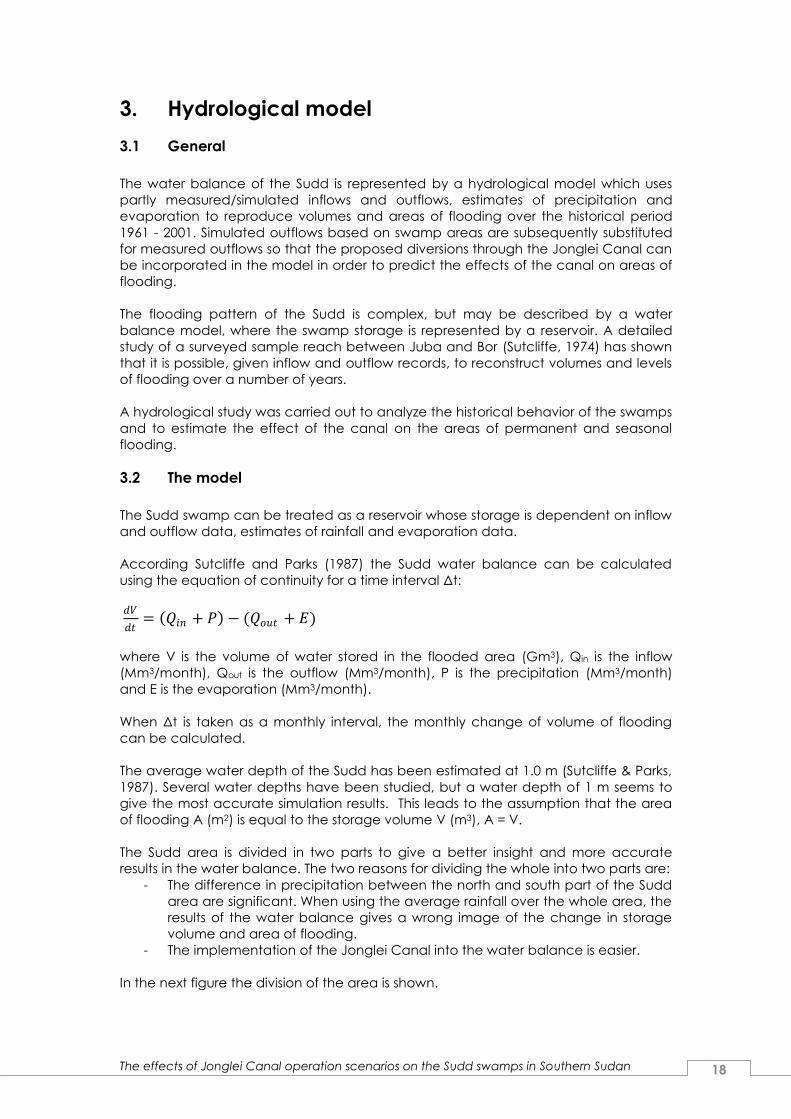
The water balance of the Sudd is represented by a hydrological model which uses
partly measured/simulated inflows and outflows, estimates of precipitation and
evaporation to reproduce volumes and areas of flooding over the historical period
1961 - 2001. Simulated outflows based on swamp areas are subsequently substituted
for measured outflows so that the proposed diversions through the Jonglei Canal can
be incorporated in the model in order to predict the effects of the canal on areas of
flooding.
The flooding pattern of the Sudd is complex, but may be described by a water
balance model, where the swamp storage is represented by a reservoir. A detailed
study of a surveyed sample reach between Juba and Bor (Sutcliffe, 1974) has shown
that it is possible, given inflow and outflow records, to reconstruct volumes and levels
of flooding over a number of years.
A hydrological study was carried out to analyze the historical behavior of the swamps
and to estimate the effect of the canal on the areas of permanent and seasonal
flooding.
3.2 The model
The Sudd swamp can be treated as a reservoir whose storage is dependent on inflow
and outflow data, estimates of rainfall and evaporation data.
According Sutcliffe and Parks (1987) the Sudd water balance can be calculated
using the equation of continuity for a time interval Δt:
𝑑𝑉
𝑑𝑡= 𝑄𝑖𝑛 + 𝑃 − (𝑄𝑜𝑢𝑡 + 𝐸)
where V is the volume of water stored in the flooded area (Gm3), Qin is the inflow
(Mm3/month), Qout is the outflow (Mm3/month), P is the precipitation (Mm3/month)
and E is the evaporation (Mm3/month).
When Δt is taken as a monthly interval, the monthly change of volume of flooding
can be calculated.
The average water depth of the Sudd has been estimated at 1.0 m (Sutcliffe & Parks,
1987). Several water depths have been studied, but a water depth of 1 m seems to
give the most accurate simulation results. This leads to the assumption that the area
of flooding A (m2) is equal to the storage volume V (m3), A = V.
The Sudd area is divided in two parts to give a better insight and more accurate
results in the water balance. The two reasons for dividing the whole into two parts are:
- The difference in precipitation between the north and south part of the Sudd
area are significant. When using the average rainfall over the whole area, the
results of the water balance gives a wrong image of the change in storage
volume and area of flooding.
- The implementation of the Jonglei Canal into the water balance is easier.
In the next figure the division of the area is shown.

The effects of Jonglei Canal operation scenarios on the Sudd swamps in Southern Sudan 19
61 km
82 km
Mongalla
Bor
Lake No
Zeraf Cuts
Malakal
Sobat River
Jo
ng
lei C
an
al
109 km
206 km
177 km
98 km
91 km
211 km
61 km
38 km105 km
1
2
Doleib Hill
Bahr el Jebel
Figure 4 The Sudd model divided in two areas
Area 1 will not be affected by the implementation of the Jonglei Canal into the water
balance, only area 2, as can be seen in the flow diagram in figure 5.
To complete the water balance for area 1 the following data is needed:
- The inflow, Qin, at Mongalla
- The outflow, Qbor, at Bor
- The precipitation in the area between Mongalla and Bor
- The evaporation in the Sudd
To complete the water balance for area 2 the following data is needed:
- The inflow, Qbor, at Bor
- The outflow, Qout, is first calculated by the extraction of the flows at Doleib Hill
from the flows at Malakal, to represent the historic water balance, and it is
next simulated to depend on the stored water volumes
- The precipitation in the area between Bor and Malakal
- The evaporation in the Sudd.
The evaporation values for both areas are assumed to be the same, because
evaporation is highly dependent on temperatures and relative humidity, which are
estimate to be almost the same due to their topographical place.

The effects of Jonglei Canal operation scenarios on the Sudd swamps in Southern Sudan 20
Area1
P1 E
Qin
Qbor
Qcanal
Area2
P2 E
Qout
Flow diagram
Figure 5 The flow diagram for the Sudd area, with the two sub-areas
The volume of precipitation and evaporation that is calculated in the water balance
is the amount of precipitation/evaporation multiplied by the corresponding area size
of the previous month. The equation will look like:
𝑉𝑝𝑟𝑒 ,𝑡 = 𝐴𝑡−1 ∗ 𝑃𝑡
𝑉𝑒𝑣𝑎 ,𝑡 = 𝐴𝑡−1 ∗ 𝐸𝑡
This formula does not take into account that it is possible that the precipitation that
takes place outside the existing swamp area will flow to the swamps, and influences
the size of the swamps for the next month. The reason is that the Sudd area is
relatively flat, so all the water that falls outside the swamp area, will not reach the
swamp. Another reason is that all the water that falls outside the area, already has
been evaporated before it can reach the swamps (E > P for most months).

The effects of Jonglei Canal operation scenarios on the Sudd swamps in Southern Sudan 21
Qin
Qout
P
E
Apr
Oct
h
Ap AsAs
Ap
Vs
The water balance in 3-D
Figure 6 The simulated swamp types by the water balance
In figure 6 the different swamp types that will be simulated with the use of the water
balance are shown. The permanent swamp (Ap) is the swamp size of the month April,
because this is in general the month with the lowest swamp size. The total swamp is
the swamp size of the month November, because this is in general the month with the
largest swamp size. The seasonal swamp (As) is accordingly determined by the
difference between the total swamp size and the permanent swamp size:
April (yri) Permanent swamp (Ap)
October (yri) Total swamp (As) + (Ap)
Seasonal swamp = Total swamp – Permanent swamp
The effects of Jonglei Canal operation scenarios on the Sudd swamps in Southern Sudan 22
3.3 Adaptation of the hydrological model with Jonglei Canal flows
With the implementation of the Jonglei Canal three variables in the water balance
need to be adjusted for the area Bor – Malakal (area 2):
- Inflow; the flow through the canal will be subtracted from the inflow at Bor.
- Outflow; the outflow of the Sudd needs to be recalculated. This will be done
by linking the swamps sizes with the simulated outflows. Now new outflows can
be calculated based on new swamp sizes.
- Evaporation; the evaporation is highly dependent on the relative humidity of
the area. When draining the Sudd, the relative humidity will drop by an
estimate of 10 percent in the dry period (October – March)(Mohamed et al.,
2005).
With these adjustments for the different variables in the water balance the swamp
sizes for different canal flow scenarios can be simulated.
3.4 Implementation of the hydrological model
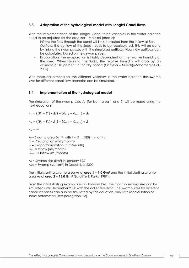
The simulation of the swamp sizes A, (for both area 1 and 2) will be made using the
next equations:
𝐴1 = 𝑃1 − 𝐸1 ∗ 𝐴0 + 𝑄𝑖𝑛 ,1 − 𝑄𝑜𝑢𝑡 ,1 + 𝐴0
𝐴2 = 𝑃2 − 𝐸2 ∗ 𝐴1 + 𝑄𝑖𝑛 ,2 − 𝑄𝑜𝑢𝑡 ,2 + 𝐴1
𝐴3 = ⋯
At = Swamp area (km2) with t = (1….480) in months
Pt = Precipitation (mm/month)
Et = Evapotranspiration (mm/month)
Qin,t = Inflow (m3/month)
Qout, t = Inflow (m3/month)
A1 = Swamp size (km2) in January 1961
A480 = Swamp size (km2) in December 2000
The initial starting swamp area A0 of area 1 = 1.0 Gm3 and the initial starting swamp
area A0 of area 2 = 15.0 Gm2 (Sutcliffe & Parks, 1987).
From the initial starting swamp area in January 1961 the monthly swamp size can be
simulated until December 2000 with the collected data. The swamp sizes for different
canal scenarios can also be simulated by this equation, only with recalculation of
some parameters (see paragraph 3.3).

The effects of Jonglei Canal operation scenarios on the Sudd swamps in Southern Sudan 23
4. Precipitation
4.1 General
The rainfall in the Sudd area varies from an average of 850 mm/yr in the northern part
(Malakal) to 1000 mm/yr in the southern part (Mongalla). The rainy season extends
from April to October, with the peak in July/August. The distribution of the rainfall in
Sudan is dominated by the position of the Intertropical Convergence Zone (ITCZ). The
ITCZ travels to as far as 20° N during the peak rainy season July to September, and
back to closer to the equator during the period November to March. Rainfall
intensities increase southward from the position of the ITCZ. The second influence on
the distribution of rainfall after the altitude is the effect of orography.
4.2 Data
The precipitation data is collected at the Global Precipitation Climatology Centre
(DWD/WZN (GPCC), 1996/2005). The GPCC analysis the spatial and temporal
distribution of global land-surface precipitation on a monthly time-scale based on in
situ observation data. The GPCC data processing steps include quality-control and
quality assurance of the station meta data and of the precipitation data,
interpolation of the station-related data to regular grids, and the calculation of the
spatial means of the 2.5°, 1° and 0.5° latitude/longitude grid box areas.
The GPCC Visualizer from the DWD creates the opportunity to select user defined
areas to collect rainfall data on different grid sizes (0.5°, 1.0° and 2.5°). Another
advantage is that the user can select monthly data over a period between 1950 and
2008 which is necessary for this study.
Figure 7 The GPCC Visualizer from the Deutsche Wetter Dienst (DWD, 2008)

The effects of Jonglei Canal operation scenarios on the Sudd swamps in Southern Sudan 24
The Sudd will be divided in two parts. The main reason is that there is a substantial
difference in the amount of precipitation between the north and south part of the
Sudd.
Mongalla – Bor
The area Mongalla – Bor is here defined as:
Longitude Latitude
31.25° – 31.75° 5.0° – 6.0°
The dataset that is applied to the area is the GPCC Land surface Full Data Product
Version 4 with a grid size of 0.5°.
Bor – Malakal
The area Mongalla – Bor is here defined as:
Longitude Latitude
30.2° – 31.75° 6.0° – 9.5°
The dataset that is applied to the area is the GPCC Land Surface Full Data Product
Version 4 with a grid size of 1.0°.
4.3 Output
The results of the analysis of the average yearly precipitation in the Sudd area are
given in the following figure.
500
600
700
800
900
1000
1100
1200
1300
1400
1961 1966 1971 1976 1981 1986 1991 1996 2001
Pre
cip
itat
ion
(m
m/y
ear
)
Time (years)
The yearly precipitation in the Sudd
Mongalla - Bor Bor - Malakal
Figure 8 The yearly precipitation in the Sudd area
The effects of Jonglei Canal operation scenarios on the Sudd swamps in Southern Sudan 25
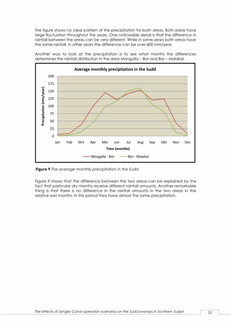
The figure shows no clear pattern of the precipitation for both areas. Both areas have
large fluctuation throughout the years. One noticeable detail is that the difference in
rainfall between the areas can be very different. While in some years both areas have
the same rainfall, in other years the difference can be over 400 mm/year.
Another way to look at the precipitation is to see what months the differences
determines the rainfall distribution in the area Mongalla – Bor and Bor – Malakal.
Figure 9 shows that the difference between the two areas can be explained by the
fact that particular dry months receive different rainfall amounts. Another remarkable
thing is that there is no difference in the rainfall amounts in the two areas in the
relative wet months. In this period they have almost the same precipitation.
0
25
50
75
100
125
150
175
200
Jan Feb Mrt Apr Mei Jun Jul Aug Sep Okt Nov Dec
Pre
cip
itat
ion
(m
m/y
ear
)
Time (months)
Average monthly precipitation in the Sudd
Mongalla - Bor Bor - Malakal
Figure 9 The average monthly precipitation in the Sudd
The effects of Jonglei Canal operation scenarios on the Sudd swamps in Southern Sudan 26
5. Evapotranspiration
5.1 Evaporation, transpiration and evapotranspiration
Evaporation
Evaporation is the process whereby liquid water is converted to water vapour and
removed from the surface. Water evaporates from a variety of surfaces, such as
lakes, rivers, and soils.
Energy is required to change the state of the molecules of water from liquid to
vapour. Direct solar radiation and the temperature of the air provide this energy. The
driving force to remove water vapour from the surface is the difference between the
water vapour pressure at the surface and that of the surrounding atmosphere. As
evaporation proceeds, the surrounding air becomes gradually saturated and the
process will slow down and might stop if the wet air is not transferred to the
atmosphere. The replacement of the saturated air with drier air depends greatly on
wind speed. Hence, solar radiation, air temperature, air humidity and wind speed are
climatological parameters to consider when assessing the evaporation process.
Transpiration
Transpiration consists of the vaporization of liquid water contained in plant tissues and
the vapour removal to the atmosphere. Crops predominately lose their water through
stomata. These are small openings on the plant leaf through which gases and water
vapour pass.
Transpiration, like direct evaporation, depends on the energy supply, vapour pressure
gradient and wind. Hence, radiation, air temperature, air humidity and wind terms
should be considered when assessing transpiration.
Evapotranspiration
Evaporation and transpiration occur simultaneously and there is no easy way of
distinguishing between the two processes. The combination of two separate
processes whereby water is lost on the one hand from the soil surface by evaporation
and on the other hand from the crop by transpiration is referred to as
evapotranspiration (ET).
5.2 Reference evapotranspiration (ET0)
The evapotranspiration rate from a reference surface is called the reference crop
evapotranspiration or reference evapotranspiration and is denoted as ETo. The
reference surface is a hypothetical grass reference crop with specific characteristics.
The concept of the reference evapotranspiration was introduced to study the
evaporative demand of the atmosphere independently of crop type, crop
development and management practices. As water is abundantly available at the
surface, soil factors do not affect ET. Relating ET to a specific surface provides a
reference to which ET from other surfaces can be related.
The only factors affecting ETo are climatic parameters. Consequently, ETo is a climatic
parameter and can be computed from weather data. ETo expresses the evaporating
power of the atmosphere at a specific location and time of the year and does not
consider the crop characteristics and soil factors.
The performance of the various calculation methods reveals the need for formulating
a standard method for the computation of ETo. The FAO Penman-Monteith method is
recommended as the sole standard method. It is a method with strong likelihood of

The effects of Jonglei Canal operation scenarios on the Sudd swamps in Southern Sudan 27
correctly predicting ETo in a wide range of locations and climates and has provision
for application in data-short situations.
5.3 FAO Penman-Monteith equation
The reference surface closely resembles an extensive surface of green grass of
uniform height, actively growing, completely shading the ground and with adequate
water. The requirements that the grass surface should be extensive and uniform result
from the assumption that all fluxes are one-dimensional upwards.
The FAO Penman-Monteith method is selected as the method by which the
evapotranspiration of this reference surface (ETo) can be determined, and as the
method which provides consistent ETo values in all regions and climates.
A panel of experts (International Commission for Irrigation and Drainage and the
World Meteorologic Organization) recommended the adoption of the Penman-
Monteith combination method as a new standard for reference evapotranspiration
and advised on procedures for calculation of the various parameters (FAO, 1998). By
defining the reference crop as a hypothetical crop with an assumed height of 0.12 m
having a surface resistance of 70 s m-1 and an albedo of 0.23 (see figure 10), closely
resembling the evaporation of an extension surface of green grass of uniform height,
actively growing and adequately watered, the FAO Penman-Monteith method was
developed. The method overcomes shortcomings of the previous FAO Penman
method and provides values more consistent with actual crop water use data
worldwide.
From the original Penman-Monteith equation and the equations of the aerodynamic
and surface resistance, the FAO Penman-Monteith method to estimate ETo can be
derived:
𝐸𝑇0 =0.408∆ 𝑅𝑛−𝐺 +𝛾
900
𝑇+273𝑢2 𝑒𝑠−𝑒𝑎
∆+𝛾 1+0.34𝑢2 (FAO, 1998)
where,
ETo = reference evapotranspiration [mm day-1]
Rn = net radiation at the crop surface [MJ m-2 day-1]
G = soil heat flux density [MJ m-2 day-1]
T = mean daily air temperature t 2 m height [°C]
u2 = wind speed at 2 m height [m s-1]
es = saturation vapour pressure [kPa]
ea = actual vapour pressure [kPa]
es - ea = saturation vapour pressure deficit [kPa]
D = slope vapour pressure curve [kPa °C-1]
g = psychometric constant [kPa °C-1]

The effects of Jonglei Canal operation scenarios on the Sudd swamps in Southern Sudan 28
The equation uses standard climatologically records of solar radiation (sunshine), air
temperature, humidity and wind speed. To ensure the integrity of computations, the
weather measurements should be made at 2 m (or converted to that height) above
an extensive surface of green grass, shading the ground and not short of water.
5.4 Calculation of ET0
The calculation of the ET0 is further explained in appendix A.
5.5 From reference evapotranspiration to actual evapotranspiration
The actual evaporation Ea is expected to be substantially lower than the reference
evaporation Eo as the basin does not exist of a reference crop (12 cm clipped grass)
with ideal moisture regimes throughout the whole year.
The actual evaporation can be calculated when dealing with the seasonal variation
of evaporation through the variation of the relative evaporation ratio Ea/Eo, which in
the irrigation literature is known as the crop coefficient Kc.
The expression to calculate the monthly actual evaporation Ea:
𝐸𝑎 = 𝐸0 ∗ 𝐾𝑐
Figure 9 Figure 10 Characteristics of the hypothetical reference crop (FAO, 1998)

The effects of Jonglei Canal operation scenarios on the Sudd swamps in Southern Sudan 29
Figure 11 The average crop factor Kc for the Sudd during three years (1995, 1999 and
2000)
The fraction Ea/E0 is determined as an average over three years (1995, 1999, 2000).
These three years were used, because these years the actual evapotranspiration was
calculated using SEBAL techniques (Mohamed, 2005). With the output from the ET0
calculator the crop factor Kc has been calculated (Figure 11).
A maximum value of Ea/Eo = 1.10 occurs in the Sudd in the middle of the wet season,
which shows that papyrus and other types of rough vegetation have an evaporation
rate more than standard clipped grass considered in the definition of E0 (Howell et al,
1988)
5.6 Results
In the next figure the average yearly actual evapotranspiration is shown for the
period 1961 – 2001.
0,40
0,50
0,60
0,70
0,80
0,90
1,00
1,10
1,20
Jan Feb Mar Apr May Jun Jul Aug Sep Oct Nov Dec
Re
lati
ve e
vap
ora
tio
n r
ate
(E a
/Eo)
Time (months)
Relative evaporation rate in the Sudd (Ea/Eo)

The effects of Jonglei Canal operation scenarios on the Sudd swamps in Southern Sudan 30
Figure 12 The yearly total actual evapotranspiration in the Sudd area
The actual evaporation shows an average increase from 1961 until 1995, with some
years that have low evaporation rates (eg. 1989). This increase is mainly caused by a
decrease in the solar radiation and relative humidity (see Appendix A, figures 32 and
33). After 1995 the evaporation rate is decreased, caused by an increase in the solar
radiation/relative humidity in the Sudd area.
1500
1550
1600
1650
1700
1750
1800
1850
1961 1966 1971 1976 1981 1986 1991 1996
Evap
otr
ansp
irat
ion
(m
m/y
ear
)
Time (years)
Yearly actual evapotranspiration in the Sudd area
The effects of Jonglei Canal operation scenarios on the Sudd swamps in Southern Sudan 31
6. Inflow
6.1 General
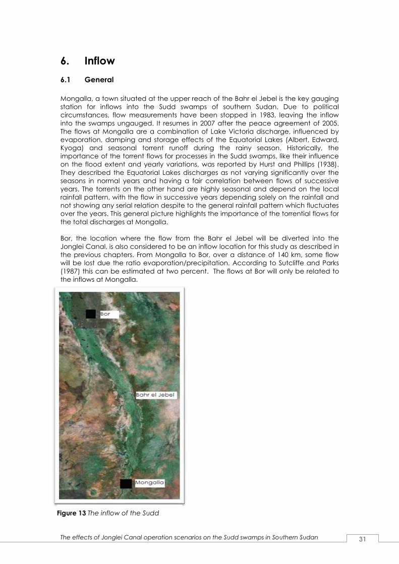
Mongalla, a town situated at the upper reach of the Bahr el Jebel is the key gauging
station for inflows into the Sudd swamps of southern Sudan. Due to political
circumstances, flow measurements have been stopped in 1983, leaving the inflow
into the swamps ungauged. It resumes in 2007 after the peace agreement of 2005.
The flows at Mongalla are a combination of Lake Victoria discharge, influenced by
evaporation, damping and storage effects of the Equatorial Lakes (Albert, Edward,
Kyoga) and seasonal torrent runoff during the rainy season. Historically, the
importance of the torrent flows for processes in the Sudd swamps, like their influence
on the flood extent and yearly variations, was reported by Hurst and Phillips (1938).
They described the Equatorial Lakes discharges as not varying significantly over the
seasons in normal years and having a fair correlation between flows of successive
years. The torrents on the other hand are highly seasonal and depend on the local
rainfall pattern, with the flow in successive years depending solely on the rainfall and
not showing any serial relation despite to the general rainfall pattern which fluctuates
over the years. This general picture highlights the importance of the torrential flows for
the total discharges at Mongalla.
Bor, the location where the flow from the Bahr el Jebel will be diverted into the
Jonglei Canal, is also considered to be an inflow location for this study as described in
the previous chapters. From Mongalla to Bor, over a distance of 140 km, some flow
will be lost due the ratio evaporation/precipitation. According to Sutcliffe and Parks
(1987) this can be estimated at two percent. The flows at Bor will only be related to
the inflows at Mongalla.
Figure 13 The inflow of the Sudd

The effects of Jonglei Canal operation scenarios on the Sudd swamps in Southern Sudan 32
6.2 Data
Mongalla
The flow series of the White Nile at Mongalla covers the period 1905-1983 which are
available from the Nile Control Staff (2000, 2007). The flows at Mongalla are equal to
the flows at Pakwach (Lake Albert outflow) plus the inflow by the torrents between
Pakwach and Mongalla. The completion of the series of Mongalla for the period
1984 – 2000 and the torrents have been carried out as follows (RIBASIM, 2008)
For the periods 1984-1992 and 1996 a 4 step approach has been used:
o Annual flows at Mongalla have been derived from regression on
Pakwach (excluding the years 1916, 1917 and 1964):
Qmongalla = 4.655 + 0.941Qpakwach + ∈
where ∈ (a,b)= is a normal deviate with mean a = 0 and standard
deviation b = 0.12.
o Annual torrent flows have been calculated for above years as the
difference between Mongalla and Pakwach;
o Monthly torrent flows have been estimated from the annual torrent
flows by scaling according to the average monthly percentage of the
annual flow;
o Monthly flow values for Mongalla have been derived from the
monthly flows at Pakwach and of the torrents.
For the periods 1993 - 1995 and 1997 - 2000 10-day mean gauge heights of Juba have
been used to estimate the gauge height at Mongalla.
Bor
The discharge at Bor will be totally dependent on the flows at Mongalla. The flows at
Mongalla will be multiplied by a factor of 0.98 to calculate to flows at Bor (Sutcliffe &
Parks, 1987).
6.3 Output
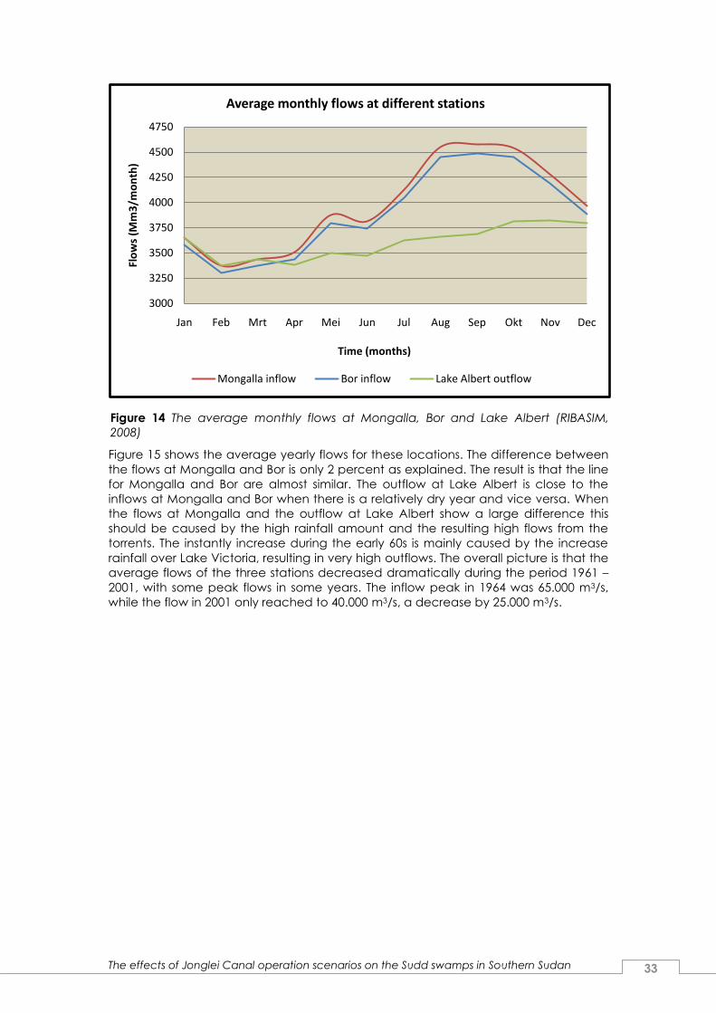
Figure 14 shows the average monthly flows for three locations. The flows at Mongalla
and Bor are described above, while the outflow at Lake Albert is included to show
the torrential influence between Lake Albert and Mongalla.
During the dry months, the three flows are almost equal. At the start of the rainy
season in April the flows at Mongalla and Bor increase substantially due to the torrents
between the outflow at Lake Albert and Mongalla. The outflow at Lake Albert shows
almost no fluctuation during the year, because the flow is highly controlled by the
outlet location Jinja of Lake Victoria.
The effects of Jonglei Canal operation scenarios on the Sudd swamps in Southern Sudan 33
Figure 15 shows the average yearly flows for these locations. The difference between
the flows at Mongalla and Bor is only 2 percent as explained. The result is that the line
for Mongalla and Bor are almost similar. The outflow at Lake Albert is close to the
inflows at Mongalla and Bor when there is a relatively dry year and vice versa. When
the flows at Mongalla and the outflow at Lake Albert show a large difference this
should be caused by the high rainfall amount and the resulting high flows from the
torrents. The instantly increase during the early 60s is mainly caused by the increase
rainfall over Lake Victoria, resulting in very high outflows. The overall picture is that the
average flows of the three stations decreased dramatically during the period 1961 –
2001, with some peak flows in some years. The inflow peak in 1964 was 65.000 m3/s,
while the flow in 2001 only reached to 40.000 m3/s, a decrease by 25.000 m3/s.
3000
3250
3500
3750
4000
4250
4500
4750
Jan Feb Mrt Apr Mei Jun Jul Aug Sep Okt Nov Dec
Flo
ws
(Mm
3/m
on
th)
Time (months)
Average monthly flows at different stations
Mongalla inflow Bor inflow Lake Albert outflow
Figure 14 The average monthly flows at Mongalla, Bor and Lake Albert (RIBASIM,
2008)

The effects of Jonglei Canal operation scenarios on the Sudd swamps in Southern Sudan 34
25000
30000
35000
40000
45000
50000
55000
60000
65000
70000
1961 1966 1971 1976 1981 1986 1991 1996
Flo
ws
(Mm
3/y
ear
)
Time (years)
Total yearly flows
Mongalla inflow Bor inflow Lake Albert outflow
Figure 15 The total yearly flows (RIBASIM, 2008)

The effects of Jonglei Canal operation scenarios on the Sudd swamps in Southern Sudan 35
7. Outflow
7.1 General
The outflow from the Sudd is in most studies (Mohamed, 2005; Sutcliffe and Parks,
1987) described as the difference between the flows of the White Nile at Malakal and
the Sobat at Doleib Hill near its mouth. In this study the same approach for the outflow
will be used. In order to simulate the outflows from the Sudd, the flows at Doleib Hill
and Malakal are needed.
Figure 16 The outflow of the Sudd
7.2 Data
Doleib Hill
The monthly flow record of the measurement station Doleib Hill at the mouth of the
Sobat River as published by the Nile Control Staff covers the period 1905 -1983. After
1983 there are no records published from the station. There will need to be a
simulation to collect this data.
Malakal
The monthly flow record for the White Nile at Malakal as published by the Nile Control
Staff covers the period 1906-2002. The monthly record has subsequently been
obtained as the average monthly percentage of the annual flow.
The effects of Jonglei Canal operation scenarios on the Sudd swamps in Southern Sudan 36
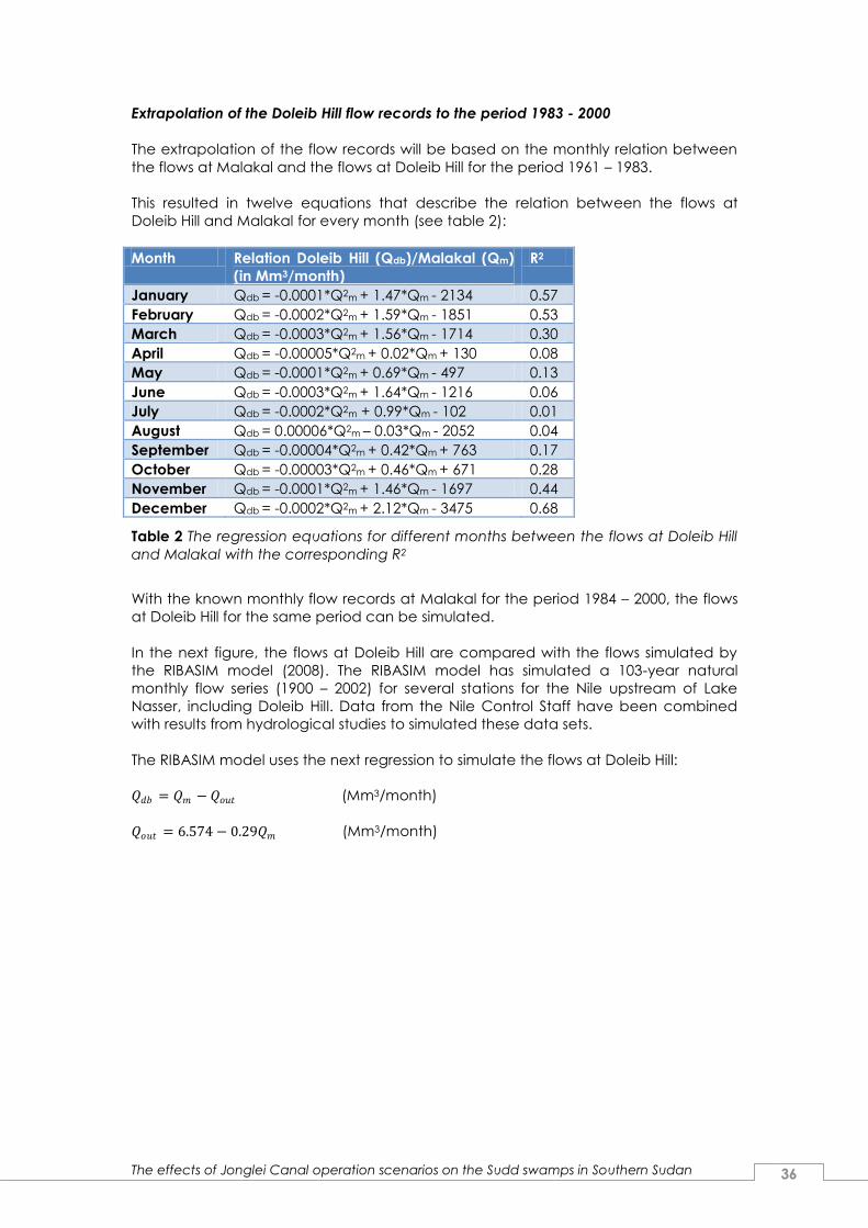
Extrapolation of the Doleib Hill flow records to the period 1983 - 2000
The extrapolation of the flow records will be based on the monthly relation between
the flows at Malakal and the flows at Doleib Hill for the period 1961 – 1983.
This resulted in twelve equations that describe the relation between the flows at
Doleib Hill and Malakal for every month (see table 2):
Month Relation Doleib Hill (Qdb)/Malakal (Qm)
(in Mm3/month)
R2
January Qdb = -0.0001*Q2m + 1.47*Qm - 2134 0.57
February Qdb = -0.0002*Q2m + 1.59*Qm - 1851 0.53
March Qdb = -0.0003*Q2m + 1.56*Qm - 1714 0.30
April Qdb = -0.00005*Q2m + 0.02*Qm + 130 0.08
May Qdb = -0.0001*Q2m + 0.69*Qm - 497 0.13
June Qdb = -0.0003*Q2m + 1.64*Qm - 1216 0.06
July Qdb = -0.0002*Q2m + 0.99*Qm - 102 0.01
August Qdb = 0.00006*Q2m – 0.03*Qm - 2052 0.04
September Qdb = -0.00004*Q2m + 0.42*Qm + 763 0.17
October Qdb = -0.00003*Q2m + 0.46*Qm + 671 0.28
November Qdb = -0.0001*Q2m + 1.46*Qm - 1697 0.44
December Qdb = -0.0002*Q2m + 2.12*Qm - 3475 0.68
Table 2 The regression equations for different months between the flows at Doleib Hill
and Malakal with the corresponding R2
With the known monthly flow records at Malakal for the period 1984 – 2000, the flows
at Doleib Hill for the same period can be simulated.
In the next figure, the flows at Doleib Hill are compared with the flows simulated by
the RIBASIM model (2008). The RIBASIM model has simulated a 103-year natural
monthly flow series (1900 – 2002) for several stations for the Nile upstream of Lake
Nasser, including Doleib Hill. Data from the Nile Control Staff have been combined
with results from hydrological studies to simulated these data sets.
The RIBASIM model uses the next regression to simulate the flows at Doleib Hill:
𝑄𝑑𝑏 = 𝑄𝑚 − 𝑄𝑜𝑢𝑡 (Mm3/month)
𝑄𝑜𝑢𝑡 = 6.574 − 0.29𝑄𝑚 (Mm3/month)

The effects of Jonglei Canal operation scenarios on the Sudd swamps in Southern Sudan 37
Figure 17 The simulated monthly flows at Doleib Hill
The results in figure 17 show the high similarities between the simulations from the
RIBASIM model as from this study. Although the monthly regression equations in this
study show low values for R2, the results are quite good compared with the regression
equation used in the RIBASIM model.
All remaining monthly flows at Doleib Hill and Malakal for the period 1984 – 2000 are
simulated. As a result the monthly Sudd outflows can be calculated for the total
period 1961 - 2000.
7.3 Output
Figure 18 shows the flows at Malakal, Doleib Hill and the outflow of the Sudd. After the
peak in the early 1960s, the outflow and the other flows have become relatively
stable. The outflow of the Sudd fluctuates around 18.000 Mm3/year for the period
1971 – 2000. The flow at Malakal is decreasing from his peak flow around 1965 until the
end of the 1980s. After that period there have been some increasing flows until 2000.
The flows at Doleib Hill show more or less the same trend, with a negative highlight in
1982.
0
500
1000
1500
2000
2500
3000
1984 1986 1988 1990 1992 1994 1996 1998 2000
Flo
ws
(Mm
3/m
on
th)
Time (years)
Simulated monthly flows at Doleib Hill (1984 - 2000)
RIBASIM Study
The effects of Jonglei Canal operation scenarios on the Sudd swamps in Southern Sudan 38
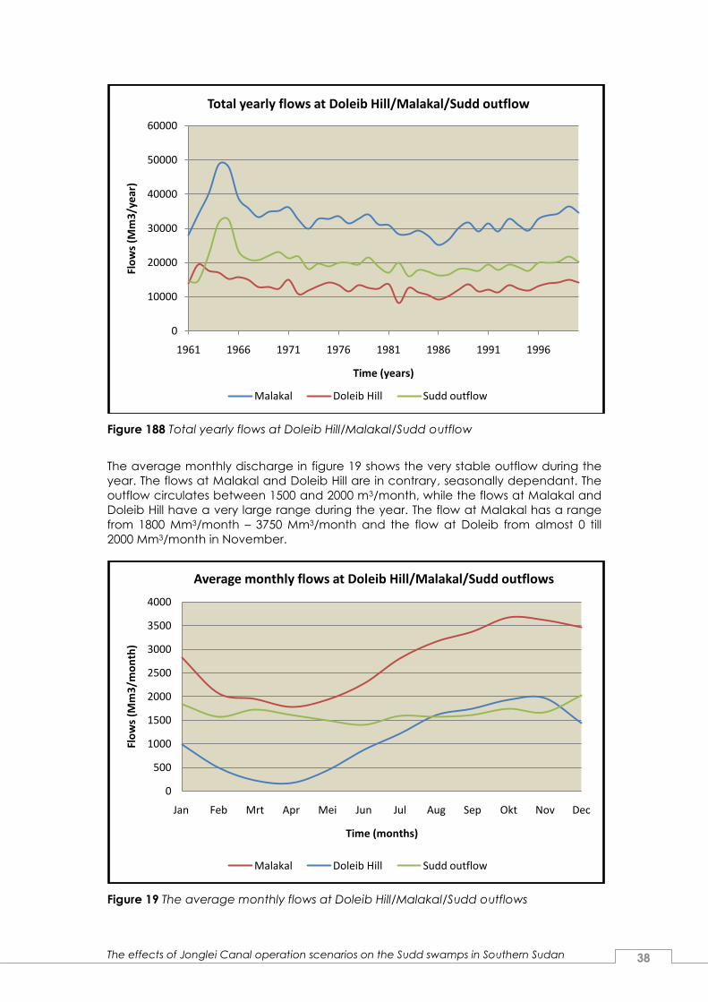
Figure 188 Total yearly flows at Doleib Hill/Malakal/Sudd outflow
The average monthly discharge in figure 19 shows the very stable outflow during the
year. The flows at Malakal and Doleib Hill are in contrary, seasonally dependant. The
outflow circulates between 1500 and 2000 m3/month, while the flows at Malakal and
Doleib Hill have a very large range during the year. The flow at Malakal has a range
from 1800 Mm3/month – 3750 Mm3/month and the flow at Doleib from almost 0 till
2000 Mm3/month in November.
Figure 19 The average monthly flows at Doleib Hill/Malakal/Sudd outflows
0
10000
20000
30000
40000
50000
60000
1961 1966 1971 1976 1981 1986 1991 1996
Flo
ws
(Mm
3/y
ear
)
Time (years)
Total yearly flows at Doleib Hill/Malakal/Sudd outflow
Malakal Doleib Hill Sudd outflow
0
500
1000
1500
2000
2500
3000
3500
4000
Jan Feb Mrt Apr Mei Jun Jul Aug Sep Okt Nov Dec
Flo
ws
(Mm
3/m
on
th)
Time (months)
Average monthly flows at Doleib Hill/Malakal/Sudd outflows
Malakal Doleib Hill Sudd outflow

The effects of Jonglei Canal operation scenarios on the Sudd swamps in Southern Sudan 39
8. The water balance
8.1 Simulation of the historic Sudd water balance
Starting from an initial storage volume of 1.0 Gm3 on 1 January 1961 for the area
between Mongalla and Bor (area 1) and 15 Gm3 for the area between Bor and
Malakal (area 2), the flooded area was simulated for monthly intervals until
December 2000. The results of the total simulated swamp sizes (area 1 + area 2) are
plotted in figure 20.
Figure 19 The total swamp size of the Sudd area
Figure 20 shows the fluctuation of the swamp size over the period 1961 – 2001. The
early 1960s have a big increase in the total swamp size, caused by the high rainfall on
Lake Victoria, resulting in a high inflow at Mongalla. After 1965 the total swamp size
fluctuates from 35 Gm2 to around 45 Gm2 in the period until 1980. After 1980 there are
three years where the total swamp size shows a big decrease. In 1984 the swamp size
recovers itself to around 35 Gm2. In the rest of the period the total swamp size is
around 30 Gm2.
The change in the swamp size is mainly caused by four variables: the inflow, outflow,
precipitation and the evaporation. One of these variables has more influence on the
change in swamp size than the other variable, but what weight have the different
variables on the change in the swamp size?
0
10
20
30
40
50
60
70
1961 1965 1969 1973 1977 1981 1985 1989 1993 1997
Swam
p s
ize
(G
m2
)
Time (years)
Total swamp size in the Sudd area
Permanent swamp Seasonal swamp
The effects of Jonglei Canal operation scenarios on the Sudd swamps in Southern Sudan 40
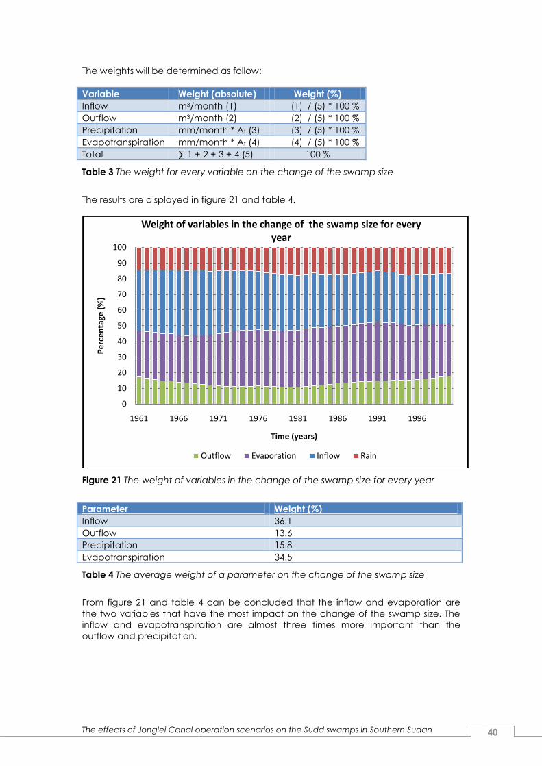
The weights will be determined as follow:
Variable Weight (absolute) Weight (%)
Inflow m3/month (1) (1) / (5) * 100 %
Outflow m3/month (2) (2) / (5) * 100 %
Precipitation mm/month * At (3) (3) / (5) * 100 %
Evapotranspiration mm/month * At (4) (4) / (5) * 100 %
Total ∑ 1 + 2 + 3 + 4 (5) 100 %
Table 3 The weight for every variable on the change of the swamp size
The results are displayed in figure 21 and table 4.
Figure 21 The weight of variables in the change of the swamp size for every year
Parameter Weight (%)
Inflow 36.1
Outflow 13.6
Precipitation 15.8
Evapotranspiration 34.5
Table 4 The average weight of a parameter on the change of the swamp size
From figure 21 and table 4 can be concluded that the inflow and evaporation are
the two variables that have the most impact on the change of the swamp size. The
inflow and evapotranspiration are almost three times more important than the
outflow and precipitation.
0
10
20
30
40
50
60
70
80
90
100
1961 1966 1971 1976 1981 1986 1991 1996
Pe
rce
nta
ge (
%)
Time (years)
Weight of variables in the change of the swamp size for every year
Outflow Evaporation Inflow Rain

The effects of Jonglei Canal operation scenarios on the Sudd swamps in Southern Sudan 41
8.2 Verification of the Sudd water balance
The verification of the water balance will be made by comparing satellite images
taken by the Landsat satellite with the calculated swamp sizes from the water
balance.
The satellite images of the Sudd area can be found of the website of the USGS
(United States Geological Survey). With the USGS Global Visualization Viewer it is
possible to download images to determine the swamp size for a specific date.
An example of an image (190 km x 190 km) is one from December 1990 (see figure
22). The figure shows only 1/3rd of the total Sudd area. The determination of the
swamp size can only be done by using three images that cover the whole area. A
raster will be set over the image to count the amount of cells that cover swamp parts.
The green colors in the figure show the swamp, while the pink color shows the non-
swamps parts. Although it is hard to really measure accurate the size of the swamp
(some parts are lighter green, some are darker green) from these satellite images, it
gives an estimate of the swamp size of that specific date.
Figure 24 Factors that determine the change of the swamp size
Figure 22 The satellite image of a part of the Sudd swamp in
December 1990
The effects of Jonglei Canal operation scenarios on the Sudd swamps in Southern Sudan 42
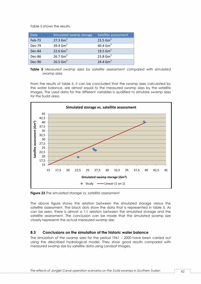
Table 5 shows the results.
Date Simulated swamp storage Satellite assessment
Feb-73 27.3 Gm3 23.5 Gm3
Dec-79 39.4 Gm3 40.4 Gm3
Dec-84 22.6 Gm3 19.5 Gm3
Dec-86 26.7 Gm3 23.8 Gm3
Dec-90 26.5 Gm3 24.4 Gm3
Table 5 Measured swamp sizes by satellite assessment compared with simulated
swamp sizes
From the results of table 5, it can be concluded that the swamp sizes calculated by
the water balance, are almost equal to the measured swamp sizes by the satellite
images. The used data for the different variables is qualified to simulate swamp sizes
for the Sudd area.
Figure 23 The simulated storage vs. satellite assessment
The above figure shows the relation between the simulated storage versus the
satellite assessment. The black dots show the data that is represented in table 5. As
can be seen, there is almost a 1:1 relation between the simulated storage and the
satellite assessment. The conclusion can be made that the simulated swamp size
closely represents the actual measured swamp size.
8.3 Conclusions on the simulation of the historic water balance
The simulation of the swamp sizes for the period 1961 – 2000 have been carried out
using the described hydrological model. They show good results compared with
measured swamp size by satellite data using Landsat images.
15
17,5
20
22,5
25
27,5
30
32,5
35
37,5
40
42,5
45
15 17,5 20 22,5 25 27,5 30 32,5 35 37,5 40 42,5 45
Sate
llite
ass
ess
me
nt
(Gm
3 )
Simulated swamp storage (Gm3)
Simulated storage vs. satellite assessment
Study Lineair (1 on 1)
The effects of Jonglei Canal operation scenarios on the Sudd swamps in Southern Sudan 43
The simulations of the historic water balance of the Sudd show some characteristic
results for certain periods. These periods can be divided into four groups:
1. 1961 – 1964 The increase of the total swamp size by almost 300 % from an
initial 15.0 Gm3 to a maximum of over 60 Gm3. The effects on the seasonal and
permanent are quite similar for that period.
2. 1965 – 1978 After the high decrease of the total swamp size from 62 Gm3 to
42 Gm3 (1964 – 1965), the total swamp size continued to decrease, although
relatively slow. The total swamp size in 1978 was around 35 Gm3. The relation
between the permanent and seasonal changed compared with the previous
period. While the relation between the permanent/seasonal swamp in the
period 1961 – 1964 around 50/50 was, the relation in the period 1965 – 1978
was changed 75/25.
3. 1979 – 1981 After 1978 there was a high decrease of the total swamp until
1981, from 35 Gm3 to 52 Gm3. In that period the relation between the
permanent/seasonal swamps changed again. This time the seasonal swamp
recovered itself to a relation around 65/35. The main cause for the increased
swamp size would be the higher rainfall in the area during that period (see
figure 8, Bor – Malakal).
4. 1982 – 2000 After 1981 the total swamp size is relatively stable, fluctuating
around 30 Gm3. The relation between the permanent/seasonal swamps has
changed for the third time. This time the seasonal swamp is even smaller,
which result in a relation of around 72/25.
The verification of the simulated swamp size with the measured swamp size shows a
difference in swamp size with a maximum of 10 percent. The conclusion is that the
simulation of the historic Sudd water balance has been successful by the hydrological
model used in this study. As well can be concluded that the used data sets for the
four variables in the model (inflow, outflow, evaporation and precipitation) are quite
good simulated.
The effects of Jonglei Canal operation scenarios on the Sudd swamps in Southern Sudan 44
9. The operation of the Jonglei canal
9.1 General
The Jonglei Canal project, considered one of the most important cooperation
projects between Egypt and Sudan, was halted in 1983 as a result of the Sudanese
civil war. The primary objective of the project was to ensure the flow of 4.8 billion
cubic meters of water annually, to be equally distributed between Egypt and Sudan,
and provide a model for similar water-conservation initiatives in other areas, such as
the Mashar swamps and the swamps of the Bahr al-Ghazal area. The first stage of the
project included the digging of a canal to provide approximately 2.4 billion cubic
meters of water annually. A second canal was to double this amount, subject to
agreement with the countries of the equatorial lakes.
9.2 The effects
The Jonglei Canal was designed to bypass the Sudd and direct downstream a
proportion of the water that is 'lost' from the Nile each year by spill and evaporation in
the swamps.
The canal has not been completed, but detailed surveys were undertaken to
determine a whole range of effects, many of which will be shown to be
disadvantageous to the inhabitants of the Jonglei Area. Some of the effects are
described below (Howell et al, 1988):
The river-flooded grasslands are an essential seasonal resource during the
driest months of the year. Not only is there drinking water available in the
rivers, but the process of seasonal inundation itself produces species of grasses
which sustain the herds from about January until April. It follows that the river-
flooded grasslands are crucial to the pastoral economy at this time of the
year. It is, however, just these grasslands that may be reduced by the
operation of the canal.
The water benefit of the canal downstream will be around 4 Gm³/yr and
according to some estimates even an extra water flow of up to 10 Gm³/yr
may be reached. These quantities are a substantial percentage of the
average 'losses' by the evapotranspiration, the natural production of river-
flooded grasses being a function of the annual fluctuation in river discharge
and thus of the annual variation in area flooded.
The established fisheries of some large lakes in the Sudd are said to have been
adversely affected by increased water depth, but, overall, the flooding of the
1960s has multiplied the number of perennial lakes in the system and, thereby,
the fishing potential. A severe decrease in the discharge into the Sudd
resulting from the Jonglei canal would bring about the total disappearance of
many lakes in the papyrus zone and reduce others to the status of seasonal
lagoons, with a serious loss of year-round fish and fishing potential.
The canal will in many areas drive a barrier between wet season villages and
dry season grazing grounds along the river channels and therefore dislocate
the pastoral cycle. Many people living east of the canal will have to cross it
with their livestock when regrowth from rain-flooded grasslands is exhausted
and they have to move westwards to the river-flooded grasslands of the Nile.
The effects of Jonglei Canal operation scenarios on the Sudd swamps in Southern Sudan 45
There exists a kind of 'Jonglei Controversy'. The criticism of the environmentalists are
many but can be placed into charges that the Jonglei Canal will drastically affect
climate, groundwater recharges, silt and water quality, the destruction of fish and
changes in the lifestyle of the people. However, other studies claim that the positive
effects will counterbalance by far the negative effects.
9.3 Operation rules of the Jonglei Canal
As described above, the implementation of the Jonglei Canal will result in several
effects. To study these effects, several alternative operating rules will be examined.
The operating rules will be split into three parts:
- Fixed canal flows
- Seasonal dependent canal flows
- Extra water volume downstream
A fixed discharge during the year gives an insight on the effects on the swamp sizes
on the long term. Seasonal dependent canal flows will give actors of ‘nature’ the
opportunity to either maintain particularly the permanent or the seasonal swamp, or
protect the stakes of actors depending on these areas by regulating the flows during
the wet and dry period. The last set of scenarios will be tested, because as planned
there will be needed an extra volume of 4.8 Gm3 downstream of the Sudd.
9.4 Adjustments in the hydrological model
As described in paragraph 3.3, the hydrological model needs to be adjusted to
calculate the new swamp sizes. Three variables need to be recalculated:
Inflow
The flows through the Jonglei Canal need to be extracted from the flows at
Bor to create the new inflow:
Qin,new = Qbor – Qcanal
Outflow
The outflow of the Sudd will change as a result of the changing swamp size. To
simulate the outflow in this new situation, a relation will be made with the
monthly swamp size and the Sudd outflow. There will be made a monthly
relation, because of the seasonal cycle of the swamps. This will result in the
following monthly relation between swamp size and Sudd outflow.
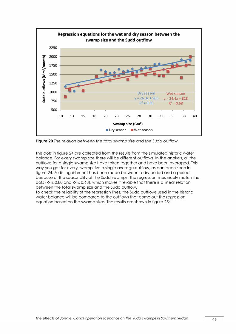
The effects of Jonglei Canal operation scenarios on the Sudd swamps in Southern Sudan 46
Figure 20 The relation between the total swamp size and the Sudd outflow
The dots in figure 24 are collected from the results from the simulated historic water
balance. For every swamp size there will be different outflows. In the analysis, all the
outflows for a single swamp size have taken together and have been averaged. This
way you get for every swamp size a single average outflow, as can been seen in
figure 24. A distinguishment has been made between a dry period and a period,
because of the seasonality of the Sudd swamps. The regression lines nicely match the
dots (R2 is 0.80 and R2 is 0.68), which makes it reliable that there is a linear relation
between the total swamp size and the Sudd outflow.
To check the reliability of the regression lines, the Sudd outflows used in the historic
water balance will be compared to the outflows that come out the regression
equation based on the swamp sizes. The results are shown in figure 25:
Dry seasony = 26.3x + 906
R² = 0.80
Wet seasony = 24.4x + 828
R² = 0.68
500
750
1000
1250
1500
1750
2000
2250
10 13 15 18 20 23 25 28 30 33 35 38 40
Sud
d o
utf
low
s (M
m3/m
on
th)
Swamp size (Gm2)
Regression equations for the wet and dry season between the swamp size and the Sudd outflow
Dry season Wet season

The effects of Jonglei Canal operation scenarios on the Sudd swamps in Southern Sudan 47
Figure 25 The regression of the Sudd outflows vs. the normal Sudd outflows
Figure 25 shows the comparison between the Sudd outflows simulated by the
regression equation and the normal Sudd outflows. As can be seen, the Sudd
outflows out the regression equation are quite smoother than the Sudd outflows used
in the historic water balance. This is caused by the effect that the regression equation
will smooth the extreme outflows in the normal Sudd outflows. The outflows show a
correlation of 0.65, which can be considered as quite good.
With the equation for the regression between the swamp size and the Sudd outflow,
the Sudd outflow can be simulated based on changed swamp sizes due to different
Jonglei canal scenarios.
Evapotranspiration
The implementation of the Jonglei Canal will result in a drop of the relative
humidity. When the whole Sudd will be drained the relative humidity will drop with
40 % in the dry season (Mohamed, 2005). Due to the fact that only about 25
percent of the normal inflow will be diverted through the Jonglei canal, it will be
assumed that the relative humidity will drop by 10 percent in the dry season. One
of the main reasons for this may be subscribed to the oasis effect. This effect is
created when wet areas are surrounded by relatively dry areas. The wind will
blow more soil moisture from the wet area to the dry area, resulting in a decrease
of the relative humidity. As a result the evapotranspiration also will increase, as
shown in figure 26.
0
500
1000
1500
2000
2500
3000
3500
4000
4500
1961 1966 1971 1976 1981 1986 1991 1996
Flo
ws
(Mm
3/m
on
th)
Time (years)
Regression Sudd outflows vs. simulated Sudd outflows
Normal Sudd outflow Regression Sudd outflow
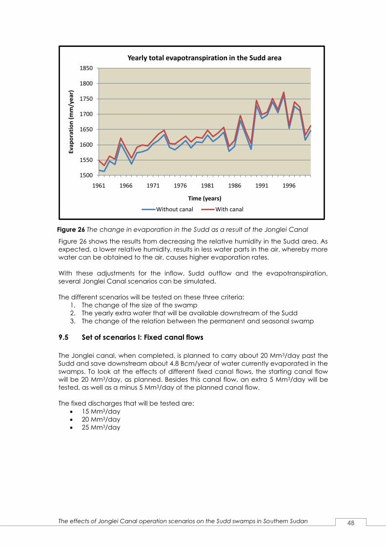
The effects of Jonglei Canal operation scenarios on the Sudd swamps in Southern Sudan 48
Figure 26 shows the results from decreasing the relative humidity in the Sudd area. As
expected, a lower relative humidity, results in less water parts in the air, whereby more
water can be obtained to the air, causes higher evaporation rates.
With these adjustments for the inflow, Sudd outflow and the evapotranspiration,
several Jonglei Canal scenarios can be simulated.
The different scenarios will be tested on these three criteria:
1. The change of the size of the swamp
2. The yearly extra water that will be available downstream of the Sudd
3. The change of the relation between the permanent and seasonal swamp
9.5 Set of scenarios I: Fixed canal flows
The Jonglei canal, when completed, is planned to carry about 20 Mm3/day past the
Sudd and save downstream about 4.8 Bcm/year of water currently evaporated in the
swamps. To look at the effects of different fixed canal flows, the starting canal flow
will be 20 Mm3/day, as planned. Besides this canal flow, an extra 5 Mm3/day will be
tested, as well as a minus 5 Mm3/day of the planned canal flow.
The fixed discharges that will be tested are:
15 Mm3/day
20 Mm3/day
25 Mm3/day
1500
1550
1600
1650
1700
1750
1800
1850
1961 1966 1971 1976 1981 1986 1991 1996
Evap
ora
tio
n (
mm
/ye
ar)
Time (years)
Yearly total evapotranspiration in the Sudd area
Without canal With canal
Figure 26 The change in evaporation in the Sudd as a result of the Jonglei Canal

The effects of Jonglei Canal operation scenarios on the Sudd swamps in Southern Sudan 49
The effects on the size of the swamps
Figure 27 The absolute swamp sizes with different fixed canal flows
Scenario
(Mm3/day)
ΔPermanent
swamp
(-%)
ΔSeasonal
swamp
(-%)
ΔTotal
swamp
(-%)
15 16.3 13.5 15.4
20 21.3 17.8 20.2
25 26.4 22.0 25.0
Table 6 The effect of different fixed canal flows on the swamp sizes
Table 6 shows the fractional changes of the different swamp types as a result of the
fixed canal flows. The permanent, seasonal and total swamps show a high linear
relation with the size of canal flow. The effects on the size of the permanent swamp
will be the highest, than the total swamp and the lowest on the seasonal swamp.
The effects on the extra available water downstream of the Sudd
Scenario
(Mm3/day)
ΔWater
volume
Dry period
(Gm3)
ΔWater
volume
Wet period
(Gm3)
ΔWater
volume
Yearly
(Gm3)
Extra
available
water (%)
15 1.9 2.1 4.0 19.7
20 2.5 2.8 5.3 26.5
25 3.1 3.5 6.6 33.3
Table 7 The effects on the extra available water downstream of the Sudd with fixed
canal flows
0
5
10
15
20
25
30
35
40
0 Mm3/day 15 Mm3/day 20 Mm3/day 25 Mm3/day
Swam
p s
ize
(G
m2 )
The absolute swamp size with different fixed canal flows
Seasonal swamp Permanent swamp Total swamp
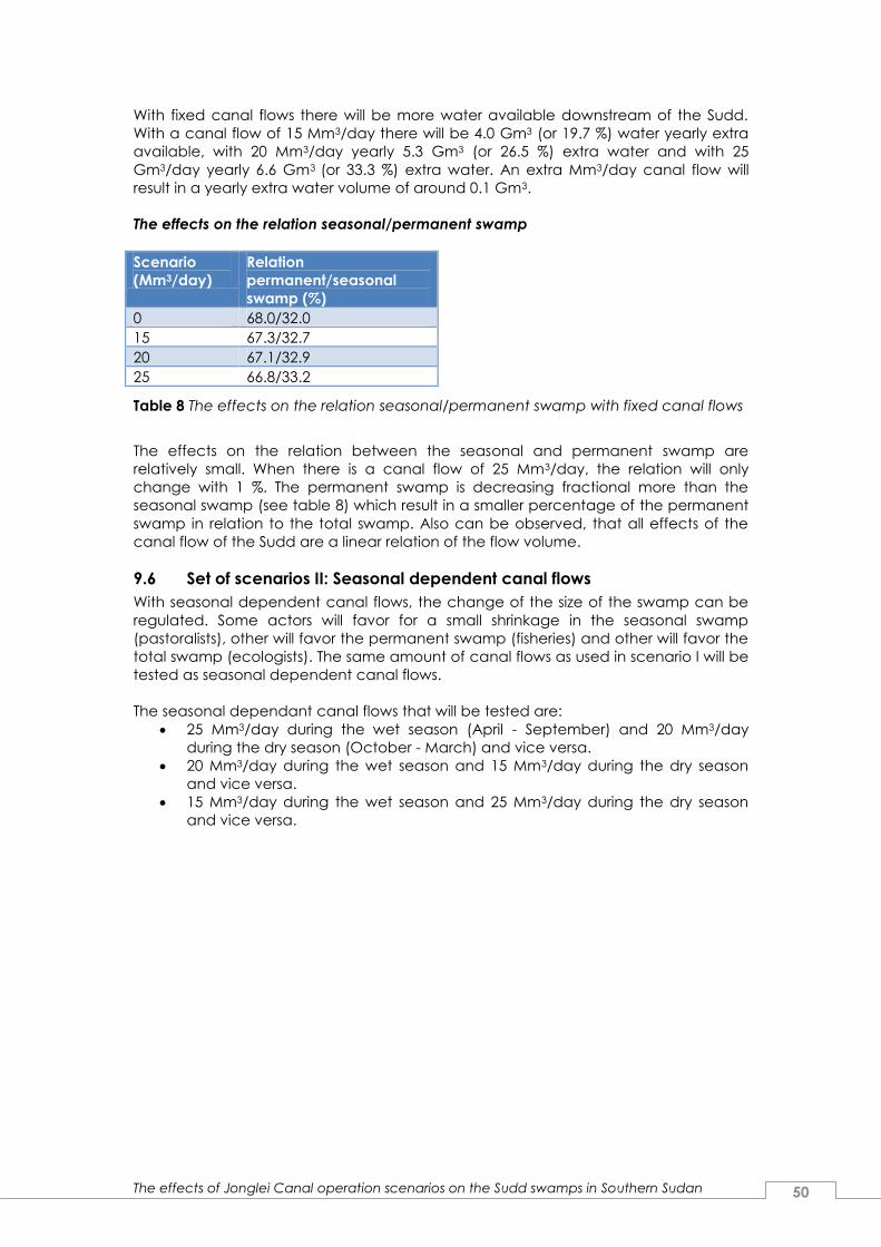
The effects of Jonglei Canal operation scenarios on the Sudd swamps in Southern Sudan 50
With fixed canal flows there will be more water available downstream of the Sudd.
With a canal flow of 15 Mm3/day there will be 4.0 Gm3 (or 19.7 %) water yearly extra
available, with 20 Mm3/day yearly 5.3 Gm3 (or 26.5 %) extra water and with 25
Gm3/day yearly 6.6 Gm3 (or 33.3 %) extra water. An extra Mm3/day canal flow will
result in a yearly extra water volume of around 0.1 Gm3.
The effects on the relation seasonal/permanent swamp
Scenario
(Mm3/day)
Relation
permanent/seasonal
swamp (%)
0 68.0/32.0
15 67.3/32.7
20 67.1/32.9
25 66.8/33.2
Table 8 The effects on the relation seasonal/permanent swamp with fixed canal flows
The effects on the relation between the seasonal and permanent swamp are
relatively small. When there is a canal flow of 25 Mm3/day, the relation will only
change with 1 %. The permanent swamp is decreasing fractional more than the
seasonal swamp (see table 8) which result in a smaller percentage of the permanent
swamp in relation to the total swamp. Also can be observed, that all effects of the
canal flow of the Sudd are a linear relation of the flow volume.
9.6 Set of scenarios II: Seasonal dependent canal flows
With seasonal dependent canal flows, the change of the size of the swamp can be
regulated. Some actors will favor for a small shrinkage in the seasonal swamp
(pastoralists), other will favor the permanent swamp (fisheries) and other will favor the
total swamp (ecologists). The same amount of canal flows as used in scenario I will be
tested as seasonal dependent canal flows.
The seasonal dependant canal flows that will be tested are:
25 Mm3/day during the wet season (April - September) and 20 Mm3/day
during the dry season (October - March) and vice versa.
20 Mm3/day during the wet season and 15 Mm3/day during the dry season
and vice versa.
15 Mm3/day during the wet season and 25 Mm3/day during the dry season
and vice versa.

The effects of Jonglei Canal operation scenarios on the Sudd swamps in Southern Sudan 51
The effects on the size of the swamps
Figure 28 The absolute swamp size with different seasonal canal flows
Scenario
(QDry-QWet)
(Mm3/day)
ΔPermanent
swamp
(-%)
ΔSeasonal
swamp
(-%)
ΔTotal
swamp
(-%)
20 - 15 19.1 13.3 17.3
15 – 20 18.3 18.0 18.2
25 – 15 22.1 13.1 19.2
15 – 25 20.5 22.5 21.1
25 – 20 24.2 17.5 22.1
20 - 25 23.4 22.3 23.1
Table 8 The effects of different seasonal canal flows on the swamp sizes
The seasonal dependent flows show the largest effects on the change of the
seasonal swamp. The change on the permanent swamp depends mainly on the total
yearly flow of Qdry + Qwet. When this is high, the fractional decrease of the permanent
swamp will also be high. The change of the seasonal swamp depends on the size of
Qwet. When this is high, the fractional decrease of the seasonal swamp will also be
high. The change on the total swamp depends, just like the permanent swamp, on
the total yearly flow of Qdry + Qwet.
0
5
10
15
20
25
30
35
40
Normal 25/15 15/25 25/20 20/25 20/15 15/20
Swam
p s
ize
(G
m2 )
Seasonal canal flows (Dry/Wet)
The absolute swamp size with different seasonal dependent canal flows
Seasonal swamp Permanent swamp Total swamp

The effects of Jonglei Canal operation scenarios on the Sudd swamps in Southern Sudan 52
The effects on the extra available water downstream of the Sudd
Scenario
(QDry-QWet)
(Mm3/day)
ΔWater
volume
Dry period
(Gm3)
ΔWater
volume
Wet period
(Gm3)
ΔWater
volume
Yearly
(Gm3)
Extra
available
water (%)
20 - 15 2.2 2.3 4.5 23.1
15 – 20 2.2 2.3 4.5 23.1
25 – 15 2.5 2.8 5.3 26.5
15 – 25 2.5 2.8 5.3 26.5
25 – 20 2.8 3.0 5.8 29.9
20 - 25 2.8 3.0 5.8 29.9
Table 9 The effect on the extra available water downstream of the Sudd with
seasonal canal flows
The extra available water downstream of the Sudd depends on the average flow of
Qdry and Qwet. With an average flow of 17.5 Mm3/day (or 23.1 %) there will be 4.5 Gm3
(or 26.4 %) yearly extra available and with an average flow of 22.5 Mm3/day there will
be 5.8 Gm3 (or 29.9 %) yearly extra available.
The effects on the relation seasonal/permanent swamp
Scenario
(Qdry – Qwet)
(Mm3/day)
Relation
permanent/seasonal
swamp (%)
0 68.0/32.0
20 – 15 66.5/33.5
15 – 20 68.0/32.0
25 - 15 65.5/34.5
15 - 25 68.6/31.4
25 - 20 66.2/33.8
20 - 25 67.7/32.3
Table 10 The effects on the relation seasonal/permanent swamp for seasonal canal
flows
Again the changes on the relation seasonal/permanent swamp are relatively small.
The higher Qdry is, the higher the fraction of the seasonal is in the total swamp. When
Qwet is higher, the fraction of the permanent swamp in the total swamp will be higher.
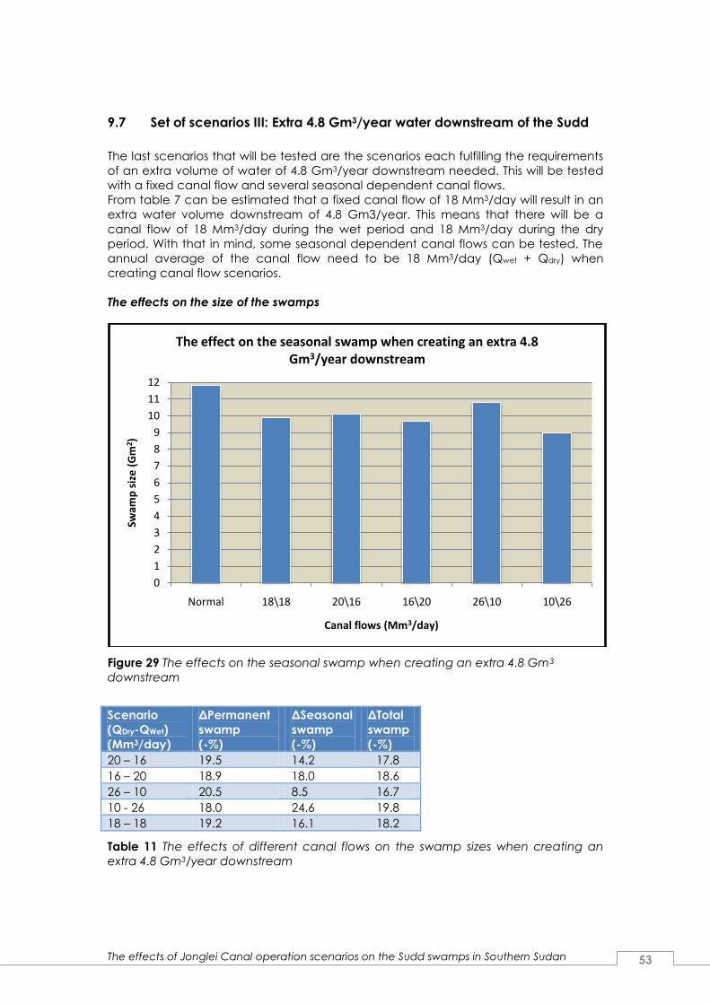
The effects of Jonglei Canal operation scenarios on the Sudd swamps in Southern Sudan 53
9.7 Set of scenarios III: Extra 4.8 Gm3/year water downstream of the Sudd
The last scenarios that will be tested are the scenarios each fulfilling the requirements
of an extra volume of water of 4.8 Gm3/year downstream needed. This will be tested
with a fixed canal flow and several seasonal dependent canal flows.
From table 7 can be estimated that a fixed canal flow of 18 Mm3/day will result in an
extra water volume downstream of 4.8 Gm3/year. This means that there will be a
canal flow of 18 Mm3/day during the wet period and 18 Mm3/day during the dry
period. With that in mind, some seasonal dependent canal flows can be tested. The
annual average of the canal flow need to be 18 Mm3/day (Qwet + Qdry) when
creating canal flow scenarios.
The effects on the size of the swamps
Figure 29 The effects on the seasonal swamp when creating an extra 4.8 Gm3
downstream
Scenario
(QDry-QWet)
(Mm3/day)
ΔPermanent
swamp
(-%)
ΔSeasonal
swamp
(-%)
ΔTotal
swamp
(-%)
20 – 16 19.5 14.2 17.8
16 – 20 18.9 18.0 18.6
26 – 10 20.5 8.5 16.7
10 - 26 18.0 24.6 19.8
18 – 18 19.2 16.1 18.2
Table 11 The effects of different canal flows on the swamp sizes when creating an
extra 4.8 Gm3/year downstream
0
1
2
3
4
5
6
7
8
9
10
11
12
Normal 18\18 20\16 16\20 26\10 10\26
Swam
p s
ize
(G
m2 )
Canal flows (Mm3/day)
The effect on the seasonal swamp when creating an extra 4.8 Gm3/year downstream

The effects of Jonglei Canal operation scenarios on the Sudd swamps in Southern Sudan 54
The scenario 10 – 26 has the highest influence on the change on the total swamp,
almost 20 %. Scenario 10 – 26 also has the highest influence on the change on the
seasonal swamp. The change of the permanent swamp will be the highest when
scenario 26 – 10 will be used, although the difference between the scenarios are
small.
From a fisherman’s perspective, scenario 10 – 26 will be in favor, because the
decrease of the permanent swamp will be at its lowest. From a pastoralist’s
perspective, scenario 26 – 10 will be in favor, because the decrease of the seasonal
swamp will be at its lowest. From an ecologist’s perspective, scenario 16 – 20 will be in
favor, because the decrease of the total swamp will be at its lowest.
The effects on the relation seasonal/permanent swamp
Table 12 The effects on the relation seasonal/permanent swamp when creating an
extra water of 4.8 Gm3/year downstream
Just like the other set of scenarios, the effects on the relation permanent/seasonal
swamp will be small. A higher Qdry results in a higher fraction of the seasonal swamp in
the total swamp. A higher Qwet results in a higher fraction of the permanent swamp in
the total swamp.
9.8 Conclusions on the operating scenarios of the Jonglei Canal
The following conclusions can be made, when looking at the results of the tests:
Fixed canal flows
A highly linear relation between size of the canal flows and the permanent,
seasonal and total swamp.
The effects on the permanent swamp size will be the highest, followed by the
total swamp size and at last the seasonal swamp size.
An extra Mm3/day canal flow will result in a yearly extra water volume of
around 0.1 Gm3.
The relation will shift from 68/32 to around 37/33.
Seasonal dependant canal flows
The strongest effects can be found on the size of the seasonal swamp.
The change on the permanent swamp depends mainly on the average yearly
canal flow of 1/2 * (Qdry + Qwet). When this is high, the fractional decrease of
the permanent swamp will also be high.
The change of the seasonal swamp depends on the size of Qwet. When this is
high, the fractional decrease of the seasonal swamp will also be high.
The change on the total swamp depends, just like the permanent swamp, on
the average yearly flow of 1/2 (Qdry + Qwet).
The relation permanent/seasonal swamp will only change small.
Scenario
(Qdry – Qwet)
(Mm3/day)
Relation
permanent/seasonal
swamp (%)
0 68.0/32.0
20 – 16 66.6/33.3
16 – 20 67.8/32.2
26 – 10 64.9/35.1
10 – 26 69.6/30.4
18 – 18 67.2/32.8

The effects of Jonglei Canal operation scenarios on the Sudd swamps in Southern Sudan 55
Extra 4.8 Gm3/year water downstream of the Sudd
The scenario 10 – 26 has the highest influence on the change on the total
swamp, almost 20 %.
Scenario 10 – 26 also has the highest influence on the change on the seasonal
swamp.
The change of the permanent swamp will be the highest when scenario 26 –
10 will be used, although the difference between the scenarios are small.
Just like the other set of scenarios, the effects on the relation
permanent/seasonal swamp will be small. A higher Qdry results in a higher
fraction of the seasonal swamp in the total swamp. A higher Qwet results in a
higher fraction of the permanent swamp in the total swamp.
In the table below the favored scenario is shown for the different actors in the Sudd
region:
Actor Favored scenario (Mm3/day)
Fisherman 10 – 26
Pastoralist 26 - 10
Ecologist 16 - 20
Table 13 The favored scenario for different actors
As can be seen, the actors have different favored scenarios. This means that there is
not one scenario that will fit every actors interests. The best scenario will be reached
when actors will drop some of their criteria.

The effects of Jonglei Canal operation scenarios on the Sudd swamps in Southern Sudan 56
10. Discussions & Recommendations
10.1 Discussions
In this paragraph the used assumptions and result uncertainties will be discussed.
The research objective and question
The research objective was to minimize the effects on the change of the size
and seasonal cycle of the Sudd when analyzing different operating rules for
the Jonglei Canal. Although it is obvious that higher canal flows result in
stronger changes on the size and seasonal cycle, the objective has been
accomplished. The criteria that were used to criticize the canal scenarios
gave good insight in the overall effects on the Sudd swamps. The criteria that
gave less effects than was expected, was the change on the relation
between the permanent and seasonal swamp. The relation stayed stable for
almost all canal scenarios. The effects on the change of the size of the
different swamp sizes was expected. The results showed almost similar results
with another study (Sutcliffe & Pars, 1987), although there were different data
sets used (especially for the evapotranspiration). The effects on the extra
gained water downstream showed good results compared with the literature;
20 Mm3/day of canal flow should result in an extra water volume of 4.8 Gm3,
while at this study this was at 18 Mm3/day.
The hydrological model
The assumption was made that the average water level of the Sudd 1.0 meter
was. Although studies (Sutcliffe & Parks, 1987) have been made to study other
water levels and show that 1.0 m has been given the best results, there is still a
high uncertainty in it. This is because the size of the water level has a high
influence on the storage volume and swamp area.
In this study the Sudd area has been divided in two parts to give more
accurate results in the water balance. It could be that when the Sudd is taken
as a whole, the results show better similarities with the reality.
The last discussion point in the hydrological model was the definition of the
different swamp types. The permanent swamp was defined as the lowest
swamp size in a certain year. The seasonal swamp was defined as the highest
swamp size minus the permanent swamp size. With these definitions certain
restrictions have been set to calculate the sizes of the types. With other
definitions, the results could show large differences.
Precipitation
The most important point of discussion is the choice for the Global
Precipitation Climatology Centre as the source of the data for the
precipitation in the Sudd. There are more sources (like the Sudan
meteorological ground stations data and the Famine Early Warning System
(FEWS)) that provide precipitation data sets for the Sudd area. The choice was
made for the GPCC, because of the high accuracy of the data sets and the
possibility to collect monthly data for the whole period 1961 – 2000.
Evapotranspiration
Although the Penman-Monteith equation the most used equation is to
calculate evapotranspiration rates, there are other equations available to
calculate the evapotranspiration (e.g. Priestley-Taylor and Hargreaves
equations (APES, 2009)). The choice was made for the Penman-Monteith

The effects of Jonglei Canal operation scenarios on the Sudd swamps in Southern Sudan 57
equation, because of the availability of data sets for the temperature, relative
humidity and sunshine hours in the Sudd area. These data can serve as input
in the Penman-Monteith equation.
To calculate the evapotranspiration the assumption was made that the
calculation for the area Bor – Malakal was represented by the averages of the
data sets at Juba and Malakal. The calculation for the area Mongalla – Bor
the assumption was made that it was represented by the averages of the
data sets only at Juba. These choices were made based on the
topographical place of these stations compared to the area.
Inflow and outflow
The regression lines for both the inflow as outflow are questionable, because
of the high uncertainties they have. Although some regression lines show low
values of R2, the lines that were picked showed the least variance with the
data points. At the end, the uncertainty will remain in the equations, but is
accepted to be part of the calculation for the inflow and outflow.
The water balance
The most important point of discussion is the verification of the Sudd swamp
sizes with the collected satellite images. It was only possible to collect satellite
images for five different dates, because the other taken images were
incompetent for further analysis. The collected images were analyzed based
on counting the parts of the images that consisted of swamps. This counting
has high uncertainties, because of the subjectivity of it. In some cases it was
impossible to distinguish swamp area with other parts. Although the
verification has high uncertainties, it was the only way to verify the simulated
swamp sizes.
Jonglei canal scenarios
Based on the results of Mohamed (2005) where the whole Sudd would be
drained and the relative humidity would drop with 40 % in the dry period, the
assumption was made that in this study the relative humidity would drop with
10 %, because the Sudd would only be drained for 25 %. This relation is highly
questionable, because the relation could not be linear as assumed.
Another point of discussion is the relation that was made between the Sudd
swamp sizes and outflows. The relation was split in two, because of the high
seasonality of the swamp sizes. There are other ways to relate these two
variables, but based on the seasonality the choice was made to use two
regression lines.
10.2 Recommendations
In this paragraph some recommendations will be made for further study.
Instead of using the Penman-Monteith equation to simulate the
evapotranspiration data, SEBAL calculations can be made to get more
accurate data about the evapotranspiration.
Other regression lines can be used for the relation between the swamp sizes
and outflow to simulate the water balance for different canal scenarios. Also
the engaging of the inflow in this relation can be something to consider.
Precipitation data sets from other sources can be used.
The effects of Jonglei Canal operation scenarios on the Sudd swamps in Southern Sudan 58
References
Allen, G. Pereira, L. Raes, D., Smith, M. (FAO) Crop evapotranspiration –
Guidelines for computing water requirements. FAO Irrigation and drainage
paper 56, Rome, Italy, 1998.
Butcher, A. D. The Sadd hydraulics. Ministry of Public Works, Cairo, Egypt, 1938.
Howell, P.P. Lock, J.M. Cobb, S.M. The Jonglei Canal: Impact and Opportunity.
Cambridge University Press, Cambridge, UK, 1988.
Hurst, H. E., & Philips, P. The hydrology of the Lake Plateau and Baher el Jebel.
The Nile Basin, vol. V, Government Press, Cairo, Egypt, 1938.
Jonglei investigation team JIT,. The Equatorial Nile Project and its effects in the
Anglo-Egyptian Sudan. Report of the Jonglei Investigation Team, Sudan
Government, Khartoum, Sudan, 1954.
Mefit-Babtie Srl. Development Studies in the Jonglei Canal Area, Final Report.
Volume 2. pp. 145-164, Khartoum, Sudan, 1983.
Migahid, A.M. Report on a Botanical Excursion to the Sudd Region. Fouad I
University Press, Cairo, Egypt. 1948.
Mohamed, Y.A. Bastiaanssen, W.G.M. Savenije, H.H.G. Spatial variability of
evaporation and moisture storage in the swamps of the upper Nile studied by
remote sensing techniques. J. Hydrology No. 289, pp 145 – 169, 2004.
Mohamed, Y.A. Bastiaanssen, W.G.M. Van den Hurk, B.J.J.M. Savenije, H.H.G.
Impact of the Sudd wetland on the Nile hydroclimatology. Water resources
research, W08420, 2005.
Mohamed, Y.A. Bastiaanssen, W.G.M. Van den Hurk, B.J.J.M. Savenije, H.H.G.
Finlayson, C.M. Evaporation from wetland versus open water: a theoretical
explanation and an application with satellite data over the Sudd wetland.
2008.
Mohamed, Y.A. Hurk, van den, B.J.J.M. Savenije, H.H.G. Bastiaanssen, W.G.M.
Hydroclimatology of the Nile: results from a regional climate model. Hydrology
and Earth System No. 9, W08420, 2005.
Penman H L. Natural evaporation from open water, bare soil and grass. Proc.
R. Soc. London Ser, pp. 120 – 146, 1984.
WL|Hydraulics et al. Hydrological boundary conditions for NFS, HAD-DSS,
RIBASIM and SOBEK modeling of the Nile upstream and downstream of
Aswan. Volume VIII, Hydrology. 2008.
Sutcliffe, J.V. A hydrological study of the Southern Sudd region of the Upper
Nile. Hydrological Science Bulletin 19. 1974.
Sutcliffe, J.V. Parks, Y.P. The hydrology of the Nile, IAHS special publication No.
5. IAHS Press, Oxfordshire, UK, 1999.
The effects of Jonglei Canal operation scenarios on the Sudd swamps in Southern Sudan 59
Internet
APES evapotranspiration models,
http://www.apesimulator.it/help/models/evapotranspiration/, May 2009.
GPCC Vizualizer, http://orias.dwd.de/GPCC/GPCC_Visualizer, December
2008.
USGS Global Visualization Viewer, http://glovis.usgs.gov/, April 2009.

The effects of Jonglei Canal operation scenarios on the Sudd swamps in Southern Sudan 60
Appendix
Appendix A Calculation of ET0
The reference evapotranspiration from meteorological data is assessed in the ET0
Calculator software by means of the FAO Penman-Monteith equation. This method
has been selected by FAO as the reference because it closely approximates grass ET0
at the location evaluated, is physically based, and explicitly incorporates both
physiological and aerodynamic parameters.
The figure above shows the parameters that are needed to calculate ET0:
Air temperature
The solar radiation absorbed by the atmosphere and the heat emitted by the earth
increase the air temperature. The sensible heat of the surrounding air transfers energy
to the crop and exerts as such a controlling influence on the rate of
evapotranspiration. In sunny, warm weather the loss of water by evapotranspiration is
greater than in cloudy and cool weather.
The daily maximum air temperature (Tmax) and daily minimum air temperature (Tmin)
are, respectively, the maximum and minimum air temperature observed during the
24-hour period, beginning at midnight. The mean daily air temperature (Tmean) is only
employed in the FAO Penman-Monteith equation to calculate the slope of the
Figure 30 The different parameters in the ETo calculator from FAO (2009)
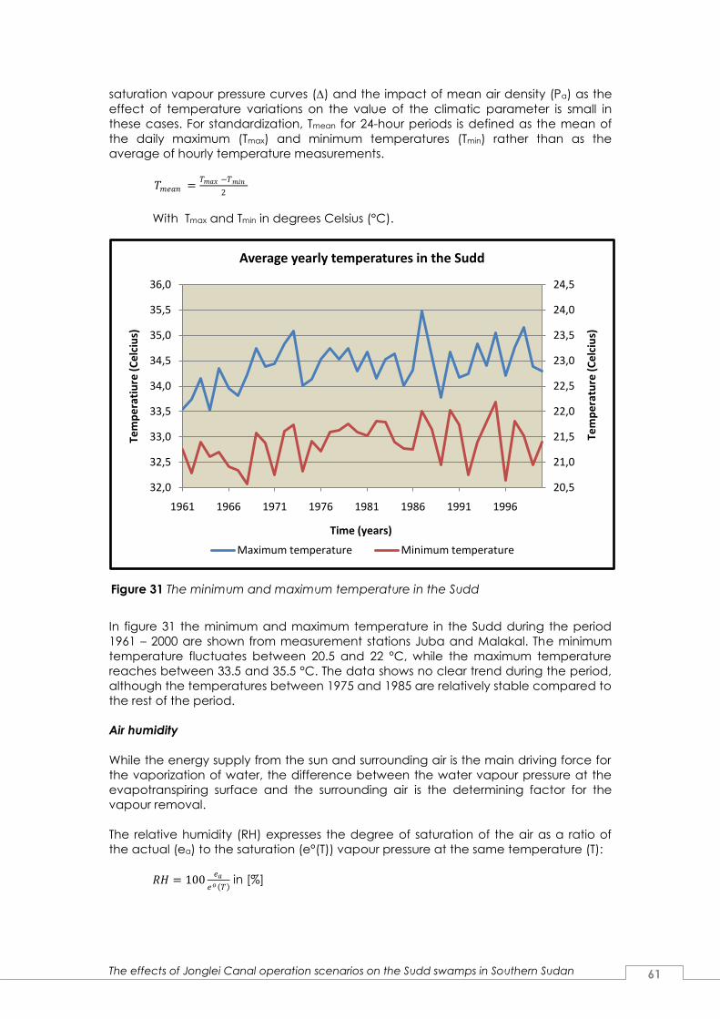
The effects of Jonglei Canal operation scenarios on the Sudd swamps in Southern Sudan 61
saturation vapour pressure curves () and the impact of mean air density (Pa) as the
effect of temperature variations on the value of the climatic parameter is small in
these cases. For standardization, Tmean for 24-hour periods is defined as the mean of
the daily maximum (Tmax) and minimum temperatures (Tmin) rather than as the
average of hourly temperature measurements.
𝑇𝑚𝑒𝑎𝑛 =𝑇𝑚𝑎𝑥 −𝑇𝑚𝑖𝑛
2
With Tmax and Tmin in degrees Celsius (°C).
In figure 31 the minimum and maximum temperature in the Sudd during the period
1961 – 2000 are shown from measurement stations Juba and Malakal. The minimum
temperature fluctuates between 20.5 and 22 °C, while the maximum temperature
reaches between 33.5 and 35.5 °C. The data shows no clear trend during the period,
although the temperatures between 1975 and 1985 are relatively stable compared to
the rest of the period.
Air humidity
While the energy supply from the sun and surrounding air is the main driving force for
the vaporization of water, the difference between the water vapour pressure at the
evapotranspiring surface and the surrounding air is the determining factor for the
vapour removal.
The relative humidity (RH) expresses the degree of saturation of the air as a ratio of
the actual (ea) to the saturation (e°(T)) vapour pressure at the same temperature (T):
𝑅𝐻 = 100𝑒𝑎
𝑒𝑜 𝑇 in [%]
20,5
21,0
21,5
22,0
22,5
23,0
23,5
24,0
24,5
32,0
32,5
33,0
33,5
34,0
34,5
35,0
35,5
36,0
1961 1966 1971 1976 1981 1986 1991 1996
Tem
pe
ratu
re (
Ce
lciu
s)
Tem
pe
rati
ure
(C
elc
ius)
Time (years)
Average yearly temperatures in the Sudd
Maximum temperature Minimum temperature
Figuur 21
Figure 31 The minimum and maximum temperature in the Sudd

The effects of Jonglei Canal operation scenarios on the Sudd swamps in Southern Sudan 62
Relative humidity is the ratio between the amount of water the air actually holds and
the amount it could hold at the same temperature. It is dimensionless and is
commonly given as a percentage. Although the actual vapour pressure might be
relatively constant throughout the day, the relative humidity fluctuates between a
maximum near sunrise and a minimum around early afternoon. The variation of the
relative humidity is the result of the fact that the saturation vapour pressure is
determined by the air temperature. As the temperature changes during the day, the
relative humidity also changes substantially.
As can been seen in figure 32 the relative humidity has dropped from 70 percent in
the early 60s around 50 percent in 1995. After 1995 the relative humidity suddenly
increased substantially setting it back on around 60 percent. This is caused by an
increase in the solar radiation, as will be shown later on.
Wind speed
The (average) daily wind speed in meters per second (m s-1) measured at 2 m above
the ground level is required. The wind speed in the Sudd is mostly unknown, and
therefore an average wind speed of 2 m/s will be used.
Sunshine and Radiation
The evapotranspiration process is determined by the amount of energy available to
vaporize water. Solar radiation is the largest energy source and is able to change
large quantities of liquid water into water vapour. The potential amount of radiation
that can reach the evaporating surface is determined by its location and time of the
year. Due to differences in the position of the sun, the potential radiation differs at
various latitudes and in different seasons.
50
52,5
55
57,5
60
62,5
65
67,5
70
72,5
75
1961 1966 1971 1976 1981 1986 1991 1996
Re
lati
ive
Hu
mid
ity
(%)
Time (years)
Average yearly relative humidity in the Sudd
Figure 32 The average yearly relative humidity in the Sudd

The effects of Jonglei Canal operation scenarios on the Sudd swamps in Southern Sudan 63
Solar radiation, Rs
If the solar radiation, Rs, is not measured, it can be calculated with the Angstrom
formula which relates solar radiation to extraterrestrial radiation and relative sunshine
duration:
𝑅𝑠 = 𝑎𝑠 + 𝑏𝑠𝑛
𝑁 𝑅𝑎
where,
Rs = solar or shortwave radiation [MJ m-2 day-1]
n = actual duration of sunshine [hour]
N = maximum possible duration of sunshine or daylight hours [hour]
n/N = relative sunshine duration [-]
Ra = extraterrestrial radiation [MJ m-2 day-1]
as regression constant, expressing the fraction of extraterrestrial radiation reaching the
earth on overcast days (n = 0)
as + bs fraction of extraterrestrial radiation reaching the earth on clear days (n = N)
Rs is expressed in the above equation in MJ m-2 day-1. The corresponding equivalent
evaporation in mm day-1 is obtained by multiplying Rs by 0.408. In the FAO Penman-
Monteith equation, radiation expressed in MJ m-2 day-1 is converted to equivalent
evaporation in mm day-1 by using a conversion factor equal to the inverse of the
latent heat of vaporization (1/ = 0.408).
Depending on atmospheric conditions and solar declination, the Angstrom values as
and bs will vary. Where no actual solar radiation data are available and no
calibration has been carried out for improved as and bs parameters, the values as =
0.25 and bs = 0.50 are recommended.
Extraterrestrial radiation, Ra
The extraterrestrial radiation, Ra, for each day of the year and for different latitudes
can be estimated from the solar constant, the solar declination and the time of the
year by:
𝑅𝑎 =24 60
𝜋𝐺𝑠𝑐𝑑𝑟 𝜔𝑠𝑠𝑖𝑛 𝜑 𝑠𝑖𝑛 𝛿 + 𝑐𝑜𝑠 𝜑 𝑐𝑜𝑠 𝛿 𝑠𝑖𝑛 𝜔𝑠
Where,
Ra = extraterrestrial radiation [MJ m-2 day-1]
Gsc = solar constant [0.0820 MJ m-2 min-1]
dr = inverse relative distance Earth-Sun [-]
s = sunset hour angle [rad]
= latitude [rad]
= solar decimation [rad]
The inverse relative distance Earth-Sun, dr, and the solar declination, , are given by:
𝑑𝑟 = 1 + 0.033𝑐𝑜𝑠 2𝜋
365𝐽
𝛿 = 0.409𝑠𝑖𝑛 2𝜋
365𝐽 − 1.39

The effects of Jonglei Canal operation scenarios on the Sudd swamps in Southern Sudan 64
where J is the number of the day in the year between 1 (1 January) and 365 or 366
(31 December).
The sunset hour angle, s, is given by:
𝜔𝑠 = 𝑎𝑟𝑐𝑐𝑜𝑠 −𝑡𝑎𝑛 𝜑 𝑡𝑎𝑛 𝛿
Ra is expressed in the above equation in MJ m-2 day-1. The corresponding equivalent
evaporation in mm day-1 is obtained by multiplying Ra by 0.408. The latitude, ,
expressed in radians is positive for the northern hemisphere and negative for the
southern hemisphere. The conversion from decimal degrees to radians is given by:
𝑅𝑎𝑑𝑖𝑎𝑛𝑠 =𝜋
180𝑑𝑒𝑐𝑖𝑚𝑎𝑙𝑑𝑒𝑔𝑟𝑒𝑒𝑠
The average yearly solar radiation shows the same pattern as the relative humidity in
the Sudd area. This is clear, because the amount of the solar radiation influence the
amount of relative humidity.
Figure 22 The average yearly solar radiation in the Sudd
All the data that was required to calculate the reference evaporation ETo for the
period 1961 – 2001 with the E0 calculator (air temperature, air humidity, sunshine and
radiation) is collected from the measurement stations Juba and Malakal.
11,2
11,3
11,4
11,5
11,6
11,7
11,8
11,9
12
12,1
12,2
12,3
1961 1966 1971 1976 1981 1986 1991 1996
Rad
iati
on
(M
J/m
2 /
day
)
Time (years)
Average yearly solar radiation in the Sudd


![CANAL [T] Canal Soth Florida](https://static.fdocuments.us/doc/165x107/55cf9803550346d03395034f/canal-t-canal-soth-florida.jpg)


![IRNA Report: [Ayod County, Jonglei State] [7- 17 August 2020]](https://static.fdocuments.us/doc/165x107/626f826b3f52c404ee255042/irna-report-ayod-county-jonglei-state-7-17-august-2020.jpg)


