The Effects of Inter-Provincial Mobility on Individuals...
47
The Effects of Inter-Provincial Mobility on Individuals’ Earnings: Panel Model Estimates for Canada by Ross Finnie No. 163 11F0019MIE No. 163 ISSN: 1205-9153 ISBN: 0-660-18374-9 Business and Labour Market Analysis 24-G. R.H. Coats Building, Ottawa, K1A 0T6 Statistics Canada (613) 951-3962 Facsimile Number (613) 951-5403 October 2001 This research was made possible by the Applied Research Branch of Human Resources Development Canada, while the Small Area and Administrative Data Division of Statistics Canada provided access to the LAD data upon which this study is based. The author also gratefully acknowledges a Social Sciences and Humanities Research Council Research Grant which was critical in earlier stages of research with the LAD data. Helpful comments have been received from Tom Courchene, Gaétan Garneau, Stéphane Gascon, Michael Hatfield, Frank Millerd, Roger Sceviour, François Vaillancourt, Allen Zeesman, and seminar participants at Guelph and Queen’s Universities, while Allen Zeesman also helped to determine the general direction of the project. Gaétan Garneau and Roger Sceviour provided excellent research assistance. This paper represents the views of the author and does not necessarily reflect the opinions of Statistics Canada. Aussi disponible en français
Transcript of The Effects of Inter-Provincial Mobility on Individuals...

The Effects of Inter-Provincial Mobility on Individuals’Earnings: Panel Model Estimates for Canada
by
Ross Finnie
No. 163
11F0019MIE No. 163ISSN: 1205-9153
ISBN: 0-660-18374-9
Business and Labour Market Analysis24-G. R.H. Coats Building, Ottawa, K1A 0T6
Statistics Canada (613) 951-3962Facsimile Number (613) 951-5403
October 2001
This research was made possible by the Applied Research Branch of Human ResourcesDevelopment Canada, while the Small Area and Administrative Data Division of StatisticsCanada provided access to the LAD data upon which this study is based. The author alsogratefully acknowledges a Social Sciences and Humanities Research Council Research Grantwhich was critical in earlier stages of research with the LAD data. Helpful comments have beenreceived from Tom Courchene, Gaétan Garneau, Stéphane Gascon, Michael Hatfield, FrankMillerd, Roger Sceviour, François Vaillancourt, Allen Zeesman, and seminar participants atGuelph and Queen’s Universities, while Allen Zeesman also helped to determine the generaldirection of the project. Gaétan Garneau and Roger Sceviour provided excellent researchassistance.
This paper represents the views of the author and does not necessarily reflect the opinions ofStatistics Canada.
Aussi disponible en français

Table of Contents
I. Introduction.......................................................................................................................................................1
II. The Existing Literature ...................................................................................................................................2
1. The Key Data Requirements and the Dearth of Existing Studies ...............................................................3
2. Previous Work Based on Longitudinal Data ...............................................................................................4
III. The Model and the Data .................................................................................................................................6
1. The Econometric Model ..............................................................................................................................6
2. A General Introduction to the LAD .............................................................................................................8
3. The Unit of Analysis and the Classification of Individuals by Mobility Status..........................................9
4. The Province of Origin and Related Language Groups ............................................................................10
5. Other Variables Included in the Models ....................................................................................................12
6. The Earnings Measure ...............................................................................................................................12
7. The Sample Selection Rules ......................................................................................................................12
8. The Age-Sex Groups..................................................................................................................................13
IV. The Empirical Findings ...............................................................................................................................13
1. Mean Earnings Patterns of Movers and Stayers.......................................................................................13
2. Level Equation Results ..............................................................................................................................15
3. The Difference Model Estimates ..............................................................................................................16
4. Testing the Pre-Move Earnings Profiles ....................................................................................................19
5. Post-Move Earnings Profiles .....................................................................................................................20
V. Conclusion ....................................................................................................................................................20
References ..........................................................................................................................................................39

Abstract
This paper presents the findings of an empirical investigation of the effects of inter-provincialmigration on individuals’ earnings based on the newly available Longitudinal AdministrativeDatabase (“LAD”). The main results are based on a difference model which estimates the effectsof mobility on (log) earnings which implicitly controls for initial earnings levels and other fixedeffects, as well as other influences captured by the regressors included in the models. Inter-provincial mobility is found to be associated with statistically significant and in many casesquantitatively substantial changes in individuals’ earnings, with these effects varying by age, sex,and province of origin. Pre- and post-move earnings profiles are also analysed, offering supportfor the validity of the difference model approach and indicating that movers are quicklyintegrated into local labour markets after their moves. Implications are discussed and possibledirections for future research are suggested.
Keywords: Earnings models, human capital, migration, fixed effects models


Analytical Studies Branch - Research Paper Series Statistics Canada No. 11F0019MIE No. 163- 1 -
I. Introduction
There are many interesting and important questions relating to inter-provincial mobility, from thedescriptive, through the analytical, to the directly policy-related. What is the general extent andspecific direction of inter-provincial mobility flows (gross and net) and how do more recent patternscompare to earlier ones? How do mobility rates vary with individual characteristics such as age,marital status, the presence of children, labour market status, level of education, and occupation.How do environmental factors such as inter-provincial differences in income levels andemployment opportunities affect the propensity to move? How much mobility leads to a returnmove and how much is permanent? What are the implications of inter-provincial mobility for inter-provincial earnings structures and regional disparities, labour market efficiency, and socialprogrammes? Furthermore, a similar set of questions could be asked regarding inter-jurisdictionalmovements elsewhere, such as inter-state or inter-regional movements in the U.S., cross-nationalmovements in the new Europe, and so on, thus placing Canadian issues pertaining to inter-provincial mobility in a broader context.
Given this importance, it is not surprising that there is by now a fairly substantial literature on inter-provincial mobility, based on both micro and aggregate data and using a variety of analyticalapproaches. We thus now know a fair amount regarding the general extent and direction of inter-provincial mobility, some of the determinants of these flows, the broad effects on individuals’earnings, certain implications for economic adjustment, and so on. Previous research has, however,been limited by the unavailability in Canada of the sort of general and extended longitudinaldatabase which is best suited to the topic. Most simply, inter-provincial migration—being a dynamicprocess—requires similarly dynamic data to be properly studied.1
The contribution of this paper is, therefore, to exploit the recently available LongitudinalAdministrative Database (“LAD”) which has been constructed by Statistics Canada from RevenueCanada tax filer records to focus on one specific aspect of the topic: the effects of inter-provincialmobility on individuals earnings.2
1 Previous work on inter-provincial mobility (thus ignoring American research on migration, but see Greenwood
[1975] for an early review of the relevant literature) includes the following. Courchene [1974], Grant andVanderkamp [1976], Lin [1995], Osberg, Gordon and Lin [1994], and Vachon and Vaillancourt [1998], documentthe extent and direction of gross out-flows, gross in-flows, and net flows, as well as the detailed patterns of theseinter-provincial movements. Models of the determinants of moving, including an important sub-literature whichfocuses on the role of fiscal variables, can be found in Day [1992], Day and Winer [1994], Dean [1992],Courchene [1970, 1974], Grant and Vanderkamp [1976], Lin [1995], Mills, Percy, and Wilson [1983], Osberg,Gordon, and Lin [1994], Robinson and Tomes [1982], Shaw [1986], Vachon and Vaillancourt [1998], and Winerand Gauthier [1982]. Investigations of the effects of inter-provincial mobility on provincial wage structures andrelated policies include Courchene [1974], Rosenbluth [1996], Shaw [1986], and Vanderkamp [1988]. Work onthe effects of inter-provincial mobility on individuals’ earnings—the topic of this paper—is reviewed below.
2 A series of companion papers (Finnie [1998a, b, c]) using the same LAD data provides descriptive (i.e., non-econometric) analyses of inter-provincial mobility in terms of the extent and direction of flows in the short-runand over longer periods on a province-by-province basis; gross outflows, gross inflows, and the associated netflows by province on an annual basis over time; and the classification of individuals into stayers and varioustypes of movers according to their longitudinal mobility behaviour and the associated income profiles. Anotherrelated paper, (Finnie [1998d]), focuses on the individual characteristics and environmental factors associatedwith inter-provincial mobility using a panel logit model approach.
Analytical Studies Branch - Research Paper Series Statistics Canada No. 11F0019MIE No. 163- 2 -
The LAD comprises a very large (ten percent) sample of Canadian tax filers followed as individualsover time and matched into family units on an annual basis, thereby providing individual andfamily-level information on incomes, taxes, and basic demographic characteristics, includingprovince of residence, in a dynamic framework.3 The LAD thus allows the researcher to effectivelyobserve the changes in earnings which occur as individuals move from one province to another,facilitating direct estimates of these effects (while controlling for other influences on earnings).Furthermore, the massive size of the LAD provides sufficiently large samples to estimate separateeffects not only by age and sex, but also by specific province (and language group)—with suchbreakdowns turning out to be of central importance to the analysis.
The analytical approach employed is conceptually quite simple: individuals are identified in termsof their inter-provincial mobility status over each three-year sequence of data, with the associatedobserved changes in earnings then identifying the effects of moving using a first difference logearnings model. For example, the earnings profiles of individuals who were in a given province inyear 1 but who moved to another province in the following year (the transition year) and then stayedin that new province the third year (thus representing a full year in the new jurisdiction) arecompared to the earnings profiles of non-movers from the same original province, with theassociated “mover” parameter identifying the average effect of moving from the province of originto another. Similar parameter estimates are derived for other types of movers: “returners”,“arrivers”, and “transients” (as defined below). Separate models and moving effects are estimatedfor men and women of four different age groups each, generating eight sets of estimates in all, withthe mobility effects allowed to vary by province (and language group) in each case.
Pre-move profiles are also analysed in order to test for pre-existing differences in the earningstrajectories of movers and non-movers which could bias the difference model estimates.Furthermore, post-move earnings profiles of movers are compared to those of non-movers of theprovinces to which they moved in order to gauge the integration of movers into their new economicsituations and test further for unobserved heterogeneity between movers and non-movers.
The paper is laid out in a straightforward fashion: the next section reviews the existing literature; thethird section presents the econometric model and the data used in the analysis; the empiricalfindings follow in the fourth section; and the final section provides a brief summary of the majorfindings and offers some suggestions for future work.
II. The Existing Literature
This section begins with a general review of the data required for any meaningful investigation ofthe effects of inter-provincial mobility on individuals’ earnings and the general shortcomings ofmost existing databases—and associated studies—in the Canadian context. In the second part, thefew existing studies based on the requisite sort of longitudinal data are reviewed.
3 Note that families and particular family members of filers are not (necessarily) followed, even as the relevant
family information is attached to the individuals’ files in each year; again, the unit of observation is theindividual with (current) family information attached in each year.

Analytical Studies Branch - Research Paper Series Statistics Canada No. 11F0019MIE No. 163- 3 -
1. The Key Data Requirements and the Dearth of Existing Studies
The primary reason for the relative lack of existing work on the effects of inter-provincial mobilityon individuals’ earnings is, as noted above, the lack of appropriate data. First, cross-sectionaldatabases (e.g., standard labour force surveys, the census) are inherently ill-suited to the analysis ofthe effects of inter-provincial mobility on earnings because they typically report only earnings levelsas of the survey date. Any comparison of the current earnings of movers and non-movers willconfound the effects of inter-provincial mobility with any other earnings-related differencesbetween movers and non-movers which are not otherwise controlled for (as discussed moreformally in the theory section below).
For example, movers might typically have higher—or lower—earnings levels to start with, and tothe degree these differences are not perfectly controlled for (via the inclusion of the relevantcontrols in a standard earnings model), any cross-sectional analysis will reflect these otherinfluences along with the mobility effects per se. Thus, cross-sectional comparisons of movers andnon-movers are likely to generate biased estimates of the effects of inter-provincial mobility onindividuals’ earnings, and it is typically impossible to identify even the direction of this bias, letalone its extent.4 In short, since inter-provincial mobility is inherently a dynamic event, similarlydynamic—or longitudinal—data are required to analyse its effects on individuals’ earnings.5
The standard longitudinal databases have, however, not been particularly appropriate to the taskeither. First-generation Canadian longitudinal databases, such as the Labour Market ActivitySurvey, have generally been both too small and too short (two to three years in length), while therecently developed Survey of Labour Income Dynamics (SLID) currently has just two years of dataavailable and will thus require some waiting before it is suitable for any detailed analysis of inter-provincial mobility.6, 7
4 Marr and Millerd [1980] is a good example of work based on cross-sectional (census) data—with precisely these
caveats not only acknowledged, but nicely explained, and unavoidably left unaddressed due to the limits of theavailable data.
5 Attempts to get around this problem by modelling what the individual would have earned had he or she notmoved using approaches which are in the spirit of the classic Heckman-type solution to sample selectionproblems may be found in Osberg, Gordon and Lin [1994], Robinson and Tomes [1982], and Nakosteen andZimmer [1980]. The problem with this methodology is that the researcher must depend on various untestableassumptions regarding the structure of earnings and related stochastic processes; it is far preferable to actually beable to observe earnings levels before and after a move—the fundamental advantage of longitudinal data.
6 For example, Osberg, Gordon, and Lin [1994] are forced to base their quite interesting analysis of inter-regionalmigration (and inter-industry mobility) using LMAS data on just 169 movers, with all moves registered in thesame one-year 1986-87 period covered by their data—with no transition year and no opportunity to look atmoves over other periods of time or the earnings dynamics of individuals before or after their moves. The SLIDis of a comparable size, and thus faces similar size limitations in the shorter-run, although this problem will beeased as further years of data are collected. Fuuthermore, the much greater array of variables available will makeit an interesting candidate for the study of various aspects of inter-provincial mobility. On the other hand, theanalysis of long-term mobility patterns using the SLID will always be limited by the fact that under currentplans, individuals will be included in the SLID for a maximum period of just six years (to then be rotated out andreplaced with others). The sample size is likely to remain a problem for any more detailed analysis, such as, forexample, the breakdown by age and sex undertaken here.
7 The National Graduates Survey databases have a semi-longitudinal element (two interviews per cohort) whichmakes them suitable for looking at issues relating to inter-provincial mobility, and the author is currently engaged
Analytical Studies Branch - Research Paper Series Statistics Canada No. 11F0019MIE No. 163- 4 -
The classic American databases (the PSID, the various NLS files, etc.)—which could in principle beused to investigate migration in the context of movements across states or regions—while certainlylong enough, have also tended to be relatively small for the purposes of studying the effects ofgeographical mobility.
Note that these oft-referenced size deficiencies stem from the fact that inter-jurisdictional mobility isa relatively rare event in any particular year for a given individual or family, while the differenteffects of mobility on earnings by age, sex, and other characteristics multiply the size requirementsdue to the relatively large number of parameters which need to be estimated. Hence, what is arelatively large database for other purposes can at the same time be quite small in the context ofestimating the effects of inter-provincial mobility on earnings.
2. Previous Work Based on Longitudinal Data
This said, there have been two quite interesting “first generation” Canadian studies of the effects ofinter-provincial mobility on individuals’ incomes carried out with early tax-based databases roughlysimilar in structure to the LAD data used here and employing conceptually similar—if somewhatmore rudimentary (non-econometric)—approaches.
Courchene [1974] uses a longitudinal database constructed from individuals’ tax files (alsoincluding unemployment insurance information) to look at the changes in individuals’ incomes from1966 to 1968, thus allowing for the assignment of each individual to a base year province (1966),providing a transition year during which a move was deemed to either have or have not occurred(1967), and permitting the observation of a full post-move year for movers and a comparable thirdyear in the original province for stayers (1968). This use of three year sequences of data is similar tothe approach used in the present study, where the concept is expanded to a continuous longitudinalsampling format.
While Courchene’s methods are restricted to simple comparisons of mean income levels, the criticalaspect of his work is that he controls for differences in initial income levels between movers andstayers by focusing on the changes in individuals’ incomes over the three year interval spanned bythe data to estimate the effects of moving—thus resolving the basic “cross-sectional” problemdescribed above. The approach is, therefore, very similar to the one used here—extended to amultivariate econometric framework and including all possible three year comparisons of data overthe entire 1982-95 period covered by the LAD data.8
Courchene, looking at males aged 15-64, finds generally positive effects of inter-provincial mobilityon individuals’ “total gross income” (the more preferable measure of labour market earnings per sewas not available for all years in his data), with the estimated aggregate effect (all workers takentogether) ranging up to an average gain of 26% in the case of men who moved from NewBrunswick. The effects are especially strong for individuals who left the have-not provinces, whileAlberta is the only province where out-migrants actually did worse than stayers (experiencing 3%
in joint work with John Burbidge of McMaster University to this end. The database is, however, obviously quitelimited in terms of the underlying population it covers (recent post-secondary graduates), meaning that the resultswill not be generalisable to the general population.
8 In his report, Courchene states the intention of undertaking such an econometric analysis in the future, perhapswith additional years of data, but these hopes were never realised.

Analytical Studies Branch - Research Paper Series Statistics Canada No. 11F0019MIE No. 163- 5 -
less income growth over the relevant interval). Conversely, individuals who left a province but thenreturned generally did worse than stayers (as well, of course, as movers who stayed away).9
Courchene’s work also resembles the present study in that he also compares the pre-move changesin the incomes of movers and stayers (again using simple comparisons of means, not econometricmodels). Not only are the pre-move levels different (thus necessitating the use of thedifference/change method), but so too are the slopes—suggesting that the income changesassociated with inter-provincial mobility were due to such individuals having steeper incomeprofiles in general as well as the effects of the move per se. However, movers’ profiles wererelatively more steep over the period covered by their moves than in the pre-move period, indicatingthat there were, in fact, gains from the moves themselves (except, again, in the case of Alberta).
Grant and Vanderkamp [1976] employ a tax-derived database similar to the one used by Courchene(again merged with unemployment insurance records) covering the period 1965-71, as well as agenerally similar methodology based on comparisons of the changes in income (total, wage, andself-employment) over time to first estimate the short-term effects (1969-70) of inter-provincialmobility on individuals’ earnings (including women along with men in their analysis) and then toextend the analysis in a number of ways.
Not surprisingly, the most directly comparable results are at least qualitatively similar to thoseobtained by Courchene. The quantitative differences in their findings (the mobility effects found byGrant and Vanderkamp are generally smaller) may be at least partly because they do not employ atransition year and compare incomes in the third year to those in the first as does Courchene—meaning that the mover-stayer comparisons are not as clean; or because they include men andwomen together in their analysis, and the female effects are much smaller than the male ones.Nevertheless, the results generally agree qualitatively in that individuals who moved from the have-not provinces appear to have generally gained from their moves, while those who left Ontario,Alberta, and British Columbia did worse than stayers. The gains are, furthermore, greater foryounger workers than older ones (as found by Courchene), and greater for men than women(although the authors express concern regarding the degree to which women are included in arepresentative manner in their samples).
Using a selected sample of individuals observed continuously over the 1966-70 period, Grant andVanderkamp also identify “long-run” (four year) migration patterns and compare the incomeprofiles of various types of movers and stayers—although the analysis is conducted in a very pooledmanner (men and women of all ages from all provinces taken together). For this more selectedsample and more aggregate analysis (while now obviously allowing for clearer comparisons of post-and pre-move incomes) they find more substantial gains for one-time movers than the simple one-year results previously revealed, diminishing returns for frequent movers, and that those whoreturned to their province of origin did worse than those who left and stayed away but (unlikeCourchene) still better than stayers. Other results are reported for inter-locality, inter-regional, andurban-rural moves, as well as by occupation.
9 The baseline group is comprised of those who stayed not just in the same province, but within the same locality,
as intra-provincial movers are separated out and analysed separately. (Intra-provincial movers generally didbetter than stayers, but not as well as inter-provincial movers).

Analytical Studies Branch - Research Paper Series Statistics Canada No. 11F0019MIE No. 163- 6 -
Finally, it is worth noting some figures regarding mobility and earnings patterns reported almost inpassing in Osberg, Gordon and Lin [1994] based on their LMAS data for the 1986-87 period. Theyfind that, overall (the results are not broken down by province of origin or any other variable exceptsex), males who moved from one region (not province) to another had significantly greater one yearincreases in earnings than did non-migrants (22.8% versus 9.0%) while female movers had onlyslightly greater increases than did female non-migrants (15.0% versus 13.2%). Their results thuspoint to sizeable returns to migration for men (in that particular year, and for a relatively smallsample), but only marginal gains for women.
These same authors also report some interesting figures regarding the reasons given for movingwhich might help explain the gender differences in returns to migration reported in their own workas well as that of others, including those reported below (the LAD data do not provide anyinformation on the reasons for a move). They find that many more males than females cited job-related reasons for moving, while females were much more likely to say they moved because theirspouse had relocated, or simply did not report a reason.10
In summary, the existing work using longitudinal data reviewed here has been based on somereasonably sound (sometimes excellent) methodological approaches and has generated a ratherinteresting body of findings regarding the effects of inter-provincial mobility on individuals’earnings. The current work is, therefore, in some sense the natural extension of these previousefforts—using a more sophisticated econometric version of the first difference approach and anupdated and rather more extended database and similarly more elaborate sample construction. Itturns out that the findings reported below are generally very consistent with these earlier findings,thus perhaps lending these newer and somewhat more refined estimates some additional credibility.
III. The Model and the Data
The first part of this section presents the econometric model and general estimation strategyemployed in the analysis, followed by a general description of the LAD database, an explanation ofthe specific unit of analysis and the classification of individuals according to their mobility status, arundown of the variables used in the estimation, and the sample selection rules.
1. The Econometric Model
Since Sjaastad [1962], economists have typically approached the topic of migration using arelatively straightforward utility maximisation framework where migration can be a means toincreasing incomes, especially labour market earnings. While it would be interesting to develop aformal rate-of-return model which explicitly took costs and the (presumed) future flow of benefitsinto account, the standard route has been to simplify the issue to the more manageable one ofestimating the changes in earnings (or some other measure of income) which occur at the point ofmigration.11
10 33.6% of the males cited one of the job related reasons (“Transferred by employer”, “To accept a job”, and “To
look for a job/work”), whereas just 17.0% of the females gave one of these reasons. Conversely, 16.2% of thefemales cited “Spouse/parent moved” and 26.4% did not state a reason, while the corresponding male figureswere just 4.2% and 21.2%, respectively.
11 See Courchene [1974] for an interesting discussion of the relation of the broader rate-of-return issue to theestimation of earnings effects.

Analytical Studies Branch - Research Paper Series Statistics Canada No. 11F0019MIE No. 163- 7 -
The problem can be represented using a standard human capital earnings model framework, wherethe log earnings of individual i in a given period (corresponding to the availability of cross-sectionaldata) can be expressed as:
(1) ln(yi) = Xiβ + αMIGi + εi
where X represents a standard set of control variables appropriate to a human capital earningsfunction, α is meant to represent the effect of having migrated from one province to another, and εis the error term.
The principal problem, however, is that migration (“MIG”) is likely to be correlated with variousearnings-related characteristics which are not otherwise controlled for in the model. Most simply, itis quite likely that migrants will have earnings levels which are generally different from those ofnon-migrants (even after controlling for the variables included in X). Let us represent thesedifferences as a set of fixed effects denoted by φ, thus yielding the following:
(2) ln(yi) = Xiβ + αMIGi + φi + ηi
The problem with any standard cross-sectional estimating equation (equation (1)) is, therefore, thatit does not take into account the likely correlation between the unobservable term φ and MIG,resulting in biased estimates of the coefficient α. This bias could be either positive or negative, andcould be large.
With the availability of longitudinal data, however, the problem can be resolved by using a firstdifferences approach:
(3) ∆ln(yi) = ∆Xiβ + αMIGi + ∆η
where, most importantly, the ∆φ term has dropped out with the differencing, and MIG is defined asan inter-provincial move taking place between two points in time spanned by the data. Unbiasedestimates of α can now be obtained by estimating standard OLS models using the differencevariables (∆η is now a well-behaved, iid error term, being a linear function of the stochasticallywell-behaved η term).
Equation (3) is basically a straightforward fixed effects model, and it is the results of the estimationof this equation which are reported below. (The findings of the estimation of equation (1) are alsopresented in order to demonstrate the bias which exists when a standard cross-sectional approach isused.) Separate equations are estimated for eight age-sex groups to allow for general differences inthe structure of earnings and different effects of migration on earnings along these dimensions,while separate parameters are estimated for out-migrants of each province and language group. Tothis author’s knowledge, this is the first use of such a model for estimating the effects of inter-provincial mobility on individual’s earnings.

Analytical Studies Branch - Research Paper Series Statistics Canada No. 11F0019MIE No. 163- 8 -
2. A General Introduction to the LAD
Since the LAD data are quite new and relatively unknown, this section offers a general descriptionof the database, with the discussion oriented towards the topic of inter-provincial mobility.12
The Longitudinal Administrative Database (“LAD”) is a 10% representative sample of Canadiantax filers followed as individuals over time and matched into family units on an annual basis, thusproviding individual and family-level information on incomes, taxes, and basic demographiccharacteristics, including province of residence, in a dynamic framework. The first year of data is1982 and the file ran through 1995 at the time this project was undertaken, thus determining theperiod covered by the analysis.
The LAD is constructed from Revenue Canada tax files, with individuals selected into the databaseaccording to a random number generator based on Social Insurance Numbers and followed overtime through the linking of records across years by the same identifier. Individuals drop out of theLAD if they become non-filers, the principal reasons being that the individual has a low income andis, therefore, not required to file (and chooses not to do so—see below); is out of the country; or hasdied. New filers (young people, immigrants, etc.) automatically refresh the database in this sameone-in-ten ratio.13
The LAD’s coverage of the adult population is very good since, unlike some other countries (suchas the U.S.) the rate of tax filing in Canada is very high: higher income Canadians are required to doso, while lower income individuals have incentives to file in order to recover income tax and otherpayroll tax deductions made throughout the year and, especially since 1986 (with the advent of thefederal sales tax credit), to receive various tax credits. The full sets of annual tax files from whichthe LAD is constructed are estimated to cover from 91% to 95% of the target adult population(official population estimates), thus comparing favourably with other survey-based databases.
The LAD thus comprises a dynamic representative sample of the adult Canadian population—dynamic in that it follows the same individuals over time, and representative in that it reflects thegeneral population in any given year and, given that most individuals file tax forms every year,representative in a longitudinal sense as well. This representativeness is especially significant in thecontext of an analysis of inter-provincial mobility, since survey based databases (as opposed to thosebased on administrative files, such as the LAD)—both cross-sectional and longitudinal—tend tohave greater problems in capturing (and following) individuals who are generally “less stable” withrespect to where they live, their job market behaviour, and other attributes, thus typicallyintroducing general sample selection and attrition biases.
12 See Finnie [1997a-g] for other discussions of the LAD data and their use in other contexts.
13 Unlike some other longitudinal databases, especially survey-based databases such as the American PSID,“replacement” observations for those who drop out of the LAD are not sought in any prescribed manner otherthan the underlying sampling scheme. In particular, there is no process whereby the number of leavers is replacedon an exact one-to-one basis, nor is there any explicit character matching of those who are added to the databasewith those who have left. Instead, all is accomplished via the simple one-in-ten sampling scheme as it drawsfrom the underlying full (and thus representative) population of (new) tax filers, who are then followed overtime.

Analytical Studies Branch - Research Paper Series Statistics Canada No. 11F0019MIE No. 163- 9 -
Furthermore, since the LAD is comprised of annual observations, most inter-provincial moves ofany importance can be identified and included in the analysis—as opposed to the length-biasedsampling which characterises files with longer intervals between observations (such as from onecensus to another).14 In short, the LAD performs well with respect to its representativenessgenerally, and is especially well suited to the study of inter-provincial mobility in this respect.15
Finally, the large number of observations on the LAD—in the range of two million in any givenyear—permits a detailed level analysis: even with the estimation broken down by age-sex group,there are enough observations to adequately identify all parameters of interest, including the effectsof leaving each specific province. (In fact, a one-in-ten sample of the full LAD file was employed tokeep the estimation numerically tractable.) Furthermore, the analysis could, in the future, be taken toa still deeper level of detail, such as estimating the models for other specific sub-groups or breakingdown the mobility effects by specific destination province as well as province of origin—with thedata standing a good chance of supporting such explorations (using the full 10% LAD whereappropriate).
3. The Unit of Analysis and the Classification of Individuals by MobilityStatus
The unit of observation used in this analysis is each three year sequence of data observed for a givenindividual. These sequences are first categorised in terms of the mobility status they represent, andthen the first and third years provide the data points which enter the first difference earnings modelspecified above.
The underlying reason for adopting this approach is that the province variable on the LAD filerepresents where the person was living at year’s end, while the earnings measure represents theamount received over the entire year. Thus, while a change in province from one year to the nextcan be identified in the obvious way, we cannot determine in which province—new or old—thesecond year’s income was earned for those who moved. The second year must, therefore, begenerally treated as a transition year.
If, however, an individual who moved from year 1 to year 2 was observed to remain in that samenew province in the third year of the given three year sequence, the last year’s income could betaken to have been earned in the new jurisdiction. (Short-run moves out of and back into theprovince of origin are thus ignored). “Year 3” post-move earnings in the new province can then becompared to the earnings received in the original province in year 1 before the move—with thesechanges compared, in turn, to the changes in earnings experienced by those who did not move. Inshort, each three year sequences permits the identification of a move, an associated “transition”year,
14 Longer-interval sample schemes would, for example, tend to under-represent shorter-term moves (which would
simply not be identified) and lead to the mis-classification of individuals who left and returned to the originalprovince within the sample period as non-movers.
15 Atkinson et al [1992] and OECD [1996] discuss the manner in which administrative databases are generallycharacterised by better coverage and less attrition than survey databases, as well as providing more reliablemeasures of income data.
Analytical Studies Branch - Research Paper Series Statistics Canada No. 11F0019MIE No. 163- 10 -
and a clear post-move year, with the associated earnings profiles of such “movers” compared tothose of stayers in order to identify the effects of earnings on individuals’ earnings.16
In this manner, individuals were classified as “stayers” (the same province in all three years),“movers” (as described above), “returners” (moved in the second year but then returned to theoriginal province in the third year), “arrivers” (in the same province the first two years but thenmoved to a new province in the third year), or “transients” (a different province each year). Eachadditional year of data facilitates a new observation in a rolling fashion: years 2 and 3 in one threeyear sequence becoming years 1 and 2 for the next, and so on. Thus, an “arriver” sequence wouldbeget a “mover” sequence if the individual stayed in that new province a second year, or a“transient” observation if the individual moved again, and so on. With the underlying LAD datarunning 1982-95 (14 years), up to 12 such observations were constructed for each individual,depending on the person’s inclusion in the original LAD file and the sample selection criteriadescribed below.
The unit of analysis (the three year rolling sequences of observations) is somewhat non-standard butwell suits the purposes at hand in that it facilitates the estimation of equation (3). It should, however,be noted that this approach obviously focuses on the short-run changes in earnings associated withmigration. Longer-term effects could be estimated by extending the analytical framework adoptedhere out to as many later periods as desired (i.e., years beyond the 3 year sequences defined above).However, the sample framework and associated selection issues would quickly become fairlycomplex, especially given the geometrically increasing number of mobility outcomes (some“stayers” will eventually move, certain more mobile individuals will eventually settle down, and soon).
The alternative approach for analysing the longer-term effects of inter-provincial mobility adoptedhere is to compare the post-move earnings profiles of movers with the profiles of individuals whowere consistently in the same province. That is, model (3) is estimated for years 3 through 5, then 4through 6—with the individual’s mobility status still defined by years 1 through 3 and imposing theadditional restriction that the individual remains in the same province through year 5 (in the firstcase) or year 6 (in the second). We thus compare the post-move earnings profiles of movers withthose of incumbents of the provinces to which they moved at comparable points in time and withsimilar sample restrictions applied to see how the former compare to the latter—in effect, a test ofthe integration of movers into their new local (provincial) labour markets.
4. The Province of Origin and Related Language Groups
The individual’s province identified in the LAD data used in this study is that in which taxes werepayable—essentially where the individual was residing at year end.17 This variable is well-suited to
16 That is, the ∆ln(y) term in equation (3) is defined as ln(y3) - ln(y1), and MIGi takes the value of unity where the
individual was living in a different province in the second year than in the first and then remained in that newprovince in the third year. As noted above, Courchene [1974] uses the very same approach of a base year, atransition year, and a post-transition year whose earnings are compared to the base year in his comparisons of themean income levels of movers and stayers.
17 Individuals living in the Yukon were included with British Columbians, while residents of the NorthwestTerritories were included with those living in Manitoba. Certain individuals with professional income have somechoice as to their tax province, but their numbers are extremely small (.01% to .06% of the sample in any year)

Analytical Studies Branch - Research Paper Series Statistics Canada No. 11F0019MIE No. 163- 11 -
the present analysis due to its being conceptually appropriate, tightly defined (including itsresidence-at-year-end specificity), and, being a key piece of information for tax purposes, itsverification by Revenue Canada. An inter-provincial move is then identified as a change in theindividual’s tax province from one year to the next.
In order to estimate mobility effects by province of origin (year 1 in the three year sequences), themodels include the relevant province indicators as regressors, along with interactions of theseprovince indicators with each of the mobility status variables, except for stayers, who represent theomitted groups against which the other mobility groups are compared. Thus, all individuals livingin, for example, Newfoundland, in the first year of a three year data sequence share that commonindicator (with Ontario as the omitted category), while the “Newfoundland mover” variablecaptures the difference in the change in earnings of those who meet the mover definition describedabove and the baseline Newfoundland stayers. A positive coefficient on this variable would thusrepresent the extra increase in earnings experienced by those who moved from Newfoundland ascompared to those who stayed in the province—the gains from migration. Other mobility statusinteractions are defined for each province in a similar manner (returners, arrivers, transients).
Given the importance of language in the Canadian context, two minority (official) languagevariables are also defined: one representing anglophones in Quebec, another representingfrancophones outside of that province.18, 19 This yields a series of province-cum-language variables.Given the particular specification used here, Ontario anglophones represent the overall omittedprovince-language category, the province indicators other than Quebec imply the use of English(omitted) and capture the differences in earnings growth rates between anglophones in thoseprovinces and the baseline English-speaking Ontario group. The Quebec variable, on the other hand,implicitly captures the effect of being a francophone in that province relative to the omitted Ontarioanglophone baseline, as the English-Quebec variable allows for differences between anglophonesand francophones in that province. Similarly, the French-ROC (“Rest of Canada”) variable capturesthe difference between francophones and anglophones in whichever province the individual residedoutside of Quebec (with that effect assumed to be constant across all provinces). The usual mobilitystatus interactions are created for the minority language groups in the same way as for the basicprovince indicators.
and the relevant choices are restricted in such a way that any one would be acceptable for the purposes of thisstudy.
18 Language is defined on the LAD file as the language of the tax form the individual completed. No other language(or ethnicity) information is available.
19 A specification along these lines was first suggested to the author in the context of another project by RonaldMeng of the University of Windsor. Note the advantage of this joint treatment of province and language tospecifications where province and language effects typically enter independently, with the inclusion of variousprovince/region indicators and a single variable to represent francophones regardless of where they live. Theconventional specification does not, in particular, allow for the anglophone minority in Quebec to exhibitdifferent behaviour from the francophone majority in that province, while the typical omnibus “French” variablecaptures an amalgam of what may be quite diverse effects for francophones inside and outside Quebec. Allowingfor minority language effects would seem to be especially important in the context of a study of inter-provincialmobility. It should be noted that the language variable pertains to that used to complete the tax form, meaningthat bilingualism and other languages are not captured by these data.

Analytical Studies Branch - Research Paper Series Statistics Canada No. 11F0019MIE No. 163- 12 -
5. Other Variables Included in the Models
A number of other control variables are included in the models, entered in terms of their values inyear 1 in the three year sequences. These include family status (unattached, childless couples,couples with children, and lone parents), area size of residence (a series of categorical variablesrunning from large urban centres to rural areas), and age and age squared (to capture the additionalage effects within each of the age-sex groups for which the model is estimated separately). Changesin these variables (true ∆X measures in equation (3)) are ignored, which is equivalent to assumingthat such changes are orthogonal to the earnings effects of inter-provincial mobility and/or that anysuch effects are small—a reasonable and convenient first approximation in the present case. Finally,a series of year dummies are entered to control for general economic conditions.
There is perhaps one notable omission on the list of regressors: education. It would certainly beinteresting to estimate the different effects of inter-provincial migration by level of education, butthe variable is simply not available on the LAD file. The same is true for occupation. At the sametime, there should be no significant bias introduced as a result of these omissions—instead, theparameter estimates simply represent the relevant effects averaged across all education levels takentogether.20
6. The Earnings Measure
The relevant income concept employed is wage and salary income plus net self-employmentincome, expressed in constant 1995 dollars and capped at the average income level of the top one-tenth percentile.21 The focus here, then, is on mobility as it relates to labour markets, as opposed toany more global definition of income.22
7. The Sample Selection Rules
Each three year sequence of observations was included in the estimation samples according to thefollowing criteria. Individuals could be included for some sequences of years but not others,depending on the specific years they are included in the LAD and pass the selection rules.
First, individuals had to be tax filers and included in the basic LAD file each year. Second, onlythose between the ages of 20 and 54 (inclusive) in the first year of each three year sequence are
20 It would be fairly essential to control for education were the analysis based on level equations—rather than the
first difference models employed here. But since education rarely changes from one year to the next (especiallywith students deleted from the analysis—see below), the effect of omitting education is mostly limited to thedifferences in the rates of change in earnings from one year to another by education level. And while earningsundoubtedly increase more (on average) for individuals with higher levels of education, these differences areunlikely to be greater than a percentage point or two over the three year sequences which form the unit ofanalysis in this study—a magnitude which is extremely small relative to the mobility effects reported below.
21 For the caps, the mean earnings value of those in the top one-tenth of the highest income percentile wascalculated for each year 1982-94, with the average of these values over all years (1982-94) then becoming thecap, applied uniformly in all years.
22 The models have also been estimated using market income—a broader concept of income than earnings. Theresults, available from the author, are generally very similar to those reported below based on the earningsmeasure.

Analytical Studies Branch - Research Paper Series Statistics Canada No. 11F0019MIE No. 163- 13 -
included. The lower age cut-off was adopted to eliminate the majority of pre-university/collegestudents and to generally restrict the analysis to decision making adults (albeit with an arbitrary cut-off), while the upper age limit is meant to focus the analysis on the working age population andavoid issues related to the transition to retirement—a dynamic worthy of study on its own. Third,full-time post-secondary students were excluded on the grounds that their mobility decisions aredriven by different factors than those obtaining for the rest of the population and would, in anyevent, be better investigated using alternative data sources. This exclusion was facilitated byimputing student status based on the relevant tax deductions available in the LAD data.23 Finally,individuals must have had positive earnings in the first and third years of each three yearsequence—corresponding to the data points represented in the estimation of model (3).
8. The Age-Sex Groups
Separate models were estimated for each of four different age groups for each sex (with age definedaccording to the first year of each three year sequence): “Entry” (20-24 inclusive), “Younger” (25-34), “Prime-Younger” (35-44), and “Prime-Older” (45-54). The reasons for restricting the analysisto those aged 20-54 have been discussed above, while the chosen categorisations are simply meantto split individuals into various major phases of the life cycle. The specific choices remainessentially arbitrary, but serve the purposes at hand: allowing for different earnings structuresgenerally, and mobility effects specifically, by age.24 Recall that age is also entered as a quadratic ineach of the separate age-sex models as a further control variable.
IV. The Empirical Findings
The presentation of the empirical findings begins with some simple mean earnings comparisons ofmovers and stayers by age-sex group and province of origin in order to establish the general natureof these profiles and to motivate the use of the difference model. These initial descriptive results arefollowed by some simple “cross-sectional” level equation results which establish the benchmarksagainst which the main difference model results may be compared, which come in the fourth part ofthe section. The estimation results for the pre- and post-move earnings profiles are presented in thelast parts of the section.
1. Mean Earnings Patterns of Movers and Stayers
Tables 1a (all individuals taken together), 1b (by sex), and 1c (by age and sex) present the meanearnings of movers, stayers, and all others combined (returners, arrivers, transients – all as definedabove) in the first (“pre-move”) and third (“post-move”) years of each sequence of observations, aswell as the related percentage change in mean earnings over these intervals.25 While this makes for agood number of some rather dense tables, some of the key patterns emerge only at this level of
23 This was a relatively elaborate exercise, as described in greater detail in Finnie [1997a, c, d, e].
24 These age groups also correspond to those used in other LAD-based work undertaken by the author (Finnie[1997a-e, g]), as well as in other joint work (Beach and Finnie [1998], Finnie and Gray [1998]), thus allowingfor comparisons across these different elements of the LAD research agenda.
25 Earnings figures are rounded to the nearest 100 dollars. Calculations based on cells with less than 15observations are not reported.

Analytical Studies Branch - Research Paper Series Statistics Canada No. 11F0019MIE No. 163- 14 -
detail. The discussion will, however, be limited to the points which are most salient to the majorthemes of this paper, with a more detailed analysis of a similar set of results offered elsewhere.26
For males (Table 1c), earnings levels and growth rates generally trace out the expected life-cyclepattern. Focusing for convenience on the modal stayer groups in each province, earnings levels aregenerally (although not uniformly) progressively higher with each age group, with the greatestdifferences being between the Entry (aged 20-24) and Younger (25-34) groups and considerablysmaller gaps between the two Prime groups (Prime-Younger, aged 35-44, and Prime-Older, aged45-54). These cross-sectional profiles are matched by the rates of earnings increases over therelevant three year intervals covered by the underlying observations, these being greatest for theEntry group (increases in the 17% to 28% range), with the profiles then flattening out to what areactually slight declines in mean earnings levels for the oldest (yet still “prime” by most labourmarket standards) age group.27
Secondly (still keeping with males), and more important to the specific topic of this paper, inter-provincial movers generally had greater increases in earnings than stayers, often significantly so,with these differences being greatest for the younger groups of workers and then tailing off for theolder groups. Entry-aged male movers had earnings increases ranging from 18% to near 100% andeven beyond in one case (Newfoundland), while stayers had average gains in the 17% to 28% rangenoted above. Younger movers had gains mostly clustered in the 15% to 28% range, versus theincreases of under 10% amongst the corresponding stayers in each province; while the patterns aremore mixed and the differences generally much smaller for the two Prime groups (especially Prime-Older).
In addition, the mover-stayer patterns vary in a systematic manner by province. The apparentadvantages of moving—larger and more consistently advantageous changes in earnings—are mostevident in the generally lowest income Atlantic provinces and also low income Saskatchewan.Conversely, movers did worse than stayers in high income Ontario, while in Alberta, another highincome jurisdiction, movers and stayers had approximately equal increases in earnings, except forthe Entry group, where movers had the advantage. On the other hand, the income-related pattern isnot perfect, as movers of all age groups did better than stayers in British Columbia, another highincome province, while the opposite holds (except for the Entry group) for Manitoba, which hasbelow average incomes.
Finally, males’ initial earnings levels also vary significantly and systematically by mobility status—with important implications for the estimation of the associated mobility effects (as discussedabove). Entry-aged male movers, for example, had lower initial earnings levels than stayers in everyprovince except Quebec—meaning that comparisons of the earnings levels of movers and stayers ata given point in time would in most cases tend to under-estimate the effects of moving. For theYounger group, however, the relative earnings levels of movers and stayers vary by province—implying a similarly mixed “cross-sectional” bias; while for the Prime age groups, movers generallyhad higher initial earnings levels than stayers, meaning that the bias would generally go in theopposite direction to that of the Entry group.
26 See Finnie [1998a, c].
27 See Finnie [1997a, b] for other work with the LAD data which focuses on cross-sectional earnings patterns andFinnie [1997c, d, e] regarding earnings dynamics.
Analytical Studies Branch - Research Paper Series Statistics Canada No. 11F0019MIE No. 163- 15 -
Females’ mean earnings levels are uniformly lower than those of males, but the gender differencesin growth rates are perhaps not as great as might have been expected. Indeed, apart from the Entrygroups, there are many cases where the women (of a given age group, in a given province) showgreater earnings increases than do men—this holding across the board for the Prime-Youngercategory. While these gender earnings patterns are interesting and important, they have beeninvestigated in other papers by the author (see the references cited above), and here we focus on themover-stayer patterns.
More important here, then, is that the female mover-stayer patterns are different from those of menin some important ways. Although Entry-aged female movers did better than stayers in everyprovince except Ontario (as for men), older female movers did worse than stayers in a relativelygreater number of cases than was true for males, and many of the mover advantages which arefound are not as great as for men, especially for the Entry and Younger groups, where the gains aregenerally greatest. It was also somewhat more common for female stayers to have had higher initialearnings levels than movers than was the case for the males.
In summary, these simple mean earnings figures suggest that moving from one province to anotherhas tended to affect individuals’ earnings to a significant degree, that there are also pre-existingdifferences in the earnings levels of movers and stayers, and that these relationships vary byprovince, age group, and sex—all of which points to the importance of using the first differenceapproach to estimating the effects of moving and of breaking the entire analysis down along thesedimensions.
2. Level Equation Results
Tables 2a (males) and 2b (females) show the results of the estimation of the benchmark “cross-sectional” model (1), where log earnings in year 3 are regressed on various control variables plusthe individual’s mobility status: stayer (the omitted category), mover, returner, arriver, and transient.In order to focus the discussion on the more cleanly defined categories, the parameter estimates forthe arriver and transient categories are not presented—with significant economies of presentationthus realised due to the fact that each category is associated with 12 additional parameters,corresponding to the province-language groups for which each set of mobility parameters has beenestimated. These results are available from the author upon request.
The estimation results for the four male groups (standard F tests confirmed the need to estimateseparate models by age group) generally look sensible with respect to the province variables (recallthat Ontario is the omitted category), family status, age and the intercept shifts for each calendaryear. As for the effects of having moved from one province to another (and then stayed in the newprovince), many of the associated earnings differences are quite large and statistically significant.
Most notable, perhaps, are the strong, positive differences in earnings levels seen for men whomoved from the Atlantic provinces, with the coefficient estimates ranging as high as .840 and theonly non-positive point estimate being for Prime-Older movers from New Brunswick.28 The mover
28 Recall that in a log earnings model, for “small” changes the coefficient estimates correspond to the percentage
effect on earnings, while such direct transformations increasingly over-approximate the effects as the coefficientestimates become larger. Nevertheless, many of these effects remain large by any standard, as can also be seen by

Analytical Studies Branch - Research Paper Series Statistics Canada No. 11F0019MIE No. 163- 16 -
coefficients are also uniformly positive and in many cases statistically significant for the two prairieprovinces, and tend towards the positive for Quebec as well, while they are almost all negative forOntario, Alberta, and British Columbia. The minority language indicators are somewhat mixed, andfurther discussion of these is reserved for the (preferred) difference models presented below.29
As for returners, their earnings are in the majority of cases lower than those of stayers, and in almostevery case below those of one-time movers (the Prime-Older group offers the most exceptions inthese regards).30 These patterns reflect a mixture of smaller earnings increases over the relevantthree year intervals plus lower earnings levels to start with.31
The female level equations are similarly well-behaved in general (province, family status, age,year), but show very different mobility effects than the male equations. The move indicators tend tobe much less positive and less statistically significant where the male effects are mostly stronglypositive (Atlantic Canada), substantially negative where the male effects are more moderatelypositive (the prairie provinces), and much more strongly negative where the male effects are alreadyin this direction (Ontario, Alberta, British Columbia). The returner effects are also generally morenegative than those found for males.
3. The Difference Model Estimates
Tables 3a and 3b present the results for the preferred difference models which implicitly control forindividuals’ initial earnings levels and other fixed effects, as well as for the other factors captured bythe regressors included in the models. The coefficient estimates should now generally be interpretedas the associated partial effects on the change in earnings (i.e., growth rates) over the three yearsequences which comprise the unit of analysis, while the mobility variables measure the change inearnings associated with moving from one province to another. The results are also portrayedgraphically, with Figures 1a and 1b showing the predicted change in earnings over the relevant three
comparing them to the coefficient estimates on some of the other variables included in the models, such as thegeneral differences in earnings level by province or the effect of being married (effects in the 0.25 range).
29 Given that the individual’s original province is included in the models, initial earnings levels (year 1) arecontrolled for at this aggregate level—for example, individuals who were in each of the Atlantic provinces willhave had generally lower earnings than individuals living in Ontario that year. Furthermore, the mover-stayercategories will reflect the associated differences in earnings levels as of the final year (year 3), including anyeffects from moving. The problem is that initial differences in earnings are, in this specification, not captured atthe individual level, and thus any such differences which are correlated with mobility status will be captured bythe move indicators—along with the true effects of moving per se. This is, of course, precisely the reason thedifference model approach is required.
30 A single “Atlantic Returner” coefficient captures the relevant effects for Newfoundland, Prince Edward Island,Nova Scotia, and New Brunswick all combined. This aggregation was necessitated by the relatively smallnumber of observations for this category for certain age groups, but the separate coefficients generated by apreliminary set of regressions were quite similar (although possessing large standard errors), indicating that thegeneral indicator represents the individual effects reasonably well.
31 Mean earnings levels in each period and the associated changes over time are not shown for this particular groupin Table 1a, but are available from the author.

Analytical Studies Branch - Research Paper Series Statistics Canada No. 11F0019MIE No. 163- 17 -
year intervals for stayers, movers, and returners, holding the effects of the other variables includedin the models constant.32
For both males and females, the models generally perform quite well with respect to the variouscontrol variables, but our discussion will focus on the relevant mobility effects. Beginning with themales, the effects of moving to another province from Atlantic Canada are now seen to be almostuniformly positive (there are just two exceptions) and in many cases very substantial, with thelargest and most statistically significant effects found for the Entry and Younger age groups, forwhom the coefficient estimates range from 0.137 (representing an increase in earnings ofapproximately 13%) to a rather astounding 0.883 (Entry group leavers from Newfoundland).
While the directions of these effects are generally similar to those of the level equations, there areclear patterns to the differences in the magnitudes of the effects obtained with the two approaches,with these differences conforming to the conjectures regarding the likely biases of the level equationestimates based on the simple mean earnings patterns seen in Table 1a. Thus, the mover effectsgenerated by the fixed effects models are larger than those of the level equations for three of the fourEntry-aged Atlantic groups, while for the other age groups all the difference equation estimatesexcept one are smaller than those obtained with the level equations.
The results for Saskatchewan are of a similar nature to those of Atlantic Canada: uniformly positiveand statistically significant coefficient estimates on the mover variable and larger effects for the twoyounger groups than the older ones. Also, once again the fixed effect estimate is greater than thelevel equation estimate for the Entry group and either basically unchanged or lower for the oldergroups.
The fixed effect results for British Columbia are, on the other hand, actually reversed in sign fromwhat was found with the level equations—the mover coefficients are now all positive, andstatistically significant for all but the oldest group, as compared to the significantly negative effectsfound for each group previously. The Alberta estimates have also shifted qualitatively to somedegree, with the coefficient estimates changing from mostly negative, and sometimes significantlyso, to generally being near zero and non-significant (the Prime-Older group goes from a negligiblepositive effect to a small negative one).
For Ontario, the sizeable and statistically significant negative mover effects obtained with the levelequations for the Entry and Younger groups are reduced in magnitude with the difference models,while the effects are rendered even more negative for the two Prime groups—these differences inthe shifting of results across the two approaches reflecting the oppositely signed biases which wereevidently operating for the younger and older age groups in the simpler specifications (again, asintimated by the mean earnings figures seen above). The Manitoba effects also shift significantlybut in different ways across the various age groups, going from moderately positive to morestrongly positive for the Entry group, from marginally positive to marginally negative for the
32 This was done by evaluating the models using the mean values of age and age squared for each group; assuming
the individual was unattached for the Entry groups, married but with no children for the Younger groups, andmarried with children for the two Prime groups; and using the omitted 1984 base year. The predicted values werethen based on the province of origin in year 1 for stayers, and adding the associated mover/arriver effects formigrants.

Analytical Studies Branch - Research Paper Series Statistics Canada No. 11F0019MIE No. 163- 18 -
Younger group, and from significantly positive to negative (but non-significant) for the two oldergroups.
Finally, the effects of leaving Quebec are now seen to be strongly positive for the two youngergroups (roughly comparable to the gains observed for Atlantic Canada), but only moderatelypositive/negative for the Prime-Younger/Older groups—at least, that is, for the francophones of thatprovince captured by the Quebec-mover variable. The departures from these “general” Quebeceffects for anglophones are captured by the English-Quebec mover variable, and the associatedcoefficient estimates point to considerably smaller gains from inter-provincial mobility for English-speaking Entry and Younger aged individuals (0.439 - 0.179 = 0.260 and 0.283 - 0.101 = 0.182),little difference for the Prime-Younger group (a point estimate of just 0.009 on the English-Quebecvariable), and a considerably more negative effect for the Prime-Older anglophone group relative tofrancophones (0.073 + 0.137).
Conversely, the French-ROC mover coefficient estimates point to a smallish advantage to movingfor Entry or Younger francophones living outside of Quebec relative to anglophones living in thesame provinces, and comparably sized negative effects for francophones over anglophones for theolder age groups. On the other hand, none of the minority language mover coefficient estimates arestatistically significant, so these results should be seen as rather speculative.33
Turning to the effects of leaving and then returning to the province of origin, the “returner”coefficient estimates are now generally smaller and less statistically significant than they were withthe level equations—suggesting that the lower earnings levels of returners seen above were largelydue to such individuals having low earnings to start with, as opposed to the effects of their mobilityper se. The sole clear pattern is that individuals who left and then returned to Ontario generally didworse than stayers, and worse than movers who then stayed in their new provinces as well (thePrime-Older group excepted), thus reinforcing the finding that men who moved from Ontario havegenerally comprised a distinct group of downwardly mobile workers (at least in terms of nominalearnings levels). Apart from this, the returner coefficient estimates tend to be negative, but are rarelystatistically significant and a fair number are actually positive—making it difficult to identify anyother general tendencies.
For females, the difference models generate quite different mobility effects than those found formales. For example, although the Atlantic province mover coefficient estimates for the Entry groupsare all substantially positive and statistically significant in all cases (except for tiny Prince EdwardIsland), as was true for males, the effects are smaller in each case. Furthermore, there is no clearpattern to the Atlantic mover effects for the three older age groups (sometimes positive, sometimesnegative, rarely significant)—in contrast to the generally positive and sometimes statisticallysignificant effects found for men.
Looking across all provinces and all age groups, the estimated female mover effects are in factoverwhelmingly (35 of 40 cases) “lower” than the male estimates—less strong where the effects forboth groups are positive, sometimes negative when the male effects are positive, and moredecidedly negative when both coefficient estimates go in this direction. From another perspective,
33 More detailed models with out-of-Quebec francophones divided into Acadians, francophone Ontarians, and
others were also estimated, but led to convergence problems and relatively imprecise coefficient estimates, andwere therefore abandoned.

Analytical Studies Branch - Research Paper Series Statistics Canada No. 11F0019MIE No. 163- 19 -
the female mover effects are considerably more likely to actually be negatively signed, especiallyfor the three older age groups, this being true in 19 of the 30 relevant cases shown in Table 3b—asopposed to negative coefficient estimates in just 11 of these cases for males.
The move-and-return effects also differ along gender lines, perhaps best summarised by noting thatfor females, 22 of the 28 coefficient estimates are negative, 7 of them significantly so, while thecorresponding figures for males are 16 and 2 respectively. From another point of view, the estimatedfemale effects are “more negative” than the male estimates in 19 of the 28 cases. In short, femalereturners generally did worse than female stayers, and relatively worse than male returners as well.
These gender patterns are obviously consistent with a family-based (“male chauvinist”) modelwhere women are more likely to move in support of their spouses’ careers, even when this results ina decline in their own earnings. They also presumably reflect the tendency for women to be morecommonly found in labour market segments—defined, for example, by occupation—whereprevious evidence has shown the benefits of migration to be more attenuated.34 These conjecturesare reinforced by the observation that the mover effects are least dissimilar for the youngest groupsof men and women—the point in the life cycle where the family context of decisions is lessimportant and gender differences in occupational patterns have not yet fully emerged.
4. Testing the Pre-Move Earnings Profiles
We now look at the pre-move changes in movers’ earnings, primarily in order to test the validity ofusing our difference models for estimating the effects of mobility on individuals’ earnings. If it werefound that movers were already on significantly different trajectories than stayers before theyactually moved (and especially if we found these profiles to resemble the mover effects estimatedacross the actual moves, as seen above), this would suggest that the move coefficients werecapturing, at least to some degree, the effects of individual heterogeneity (in the differences) ratherthan the effects of moving per se, thus requiring the appropriate adjustments to the estimates.
Tables 4a and 4b thus show the effects of adding to the fixed effects models a series of “pre-move”variables which represent the relevant intervals of those who subsequently left their homeprovince.35 Although a small number of the pre-move coefficient estimates are individuallystatistically significant, there is no clear pattern to the results, and the appropriate F-tests indicatethat the coefficients on the blocks of pre-move variables are in no case statistically significant fromzero. The other coefficient estimates (including the actual mobility indicators) are, meanwhile, littlechanged. These findings indicate that the fixed effect model approach is indeed appropriate to thetask and that the results reported above should be taken as good estimates of the effects of inter-provincial mobility on individuals’ earnings.
34 See, for example, Grant and Vanderkamp [1976].
35 More specifically, an individual identified as a mover over a given sequence of years 1 through 3 is nowidentified as a “pre-mover” over the first year of the relevant sequence and the preceding two years. Thecondition that the individual was in the same (original) province each of these years is also added so as to isolatethe heterogeneity effects from all mobility effects per se. Finally, since such observations require 5 consecutiveyears of data for given individuals, the samples were generally restricted to observations meeting this criteria soas to avoid any influences of (asymmetric) length-biased sampling.

Analytical Studies Branch - Research Paper Series Statistics Canada No. 11F0019MIE No. 163- 20 -
5. Post-Move Earnings Profiles
A similar approach is used to inspect post-move profiles, in this case comparing movers to theincumbents of the provinces to which they migrated, thereby allowing us to see how quickly moversbecame integrated into their new local labour markets and providing an additional test for omittedheterogeneity. Tables 5a and 5b thus present the results of models which include “post-move”variables for the first complete three year interval in the new province following the move. Tables6a and 6b repeat this exercise for the next (rolling) three year period (that is from the secondthrough fourth years in the new province).36
While there are again a number of statistically significant coefficient estimates for the first completethree year period in the new province, only two of these remain significant for the followingsequence of years, and in each case the relevant F test again indicates that the blocks of “post-move”coefficient estimates are not significantly different from zero. The data thus indicate that moversrapidly integrate into their new “local” labour markets and are not generally different from non-movers in any manner which might affect the fixed effect estimation results reported above.37
V. Conclusion
This paper has presented the findings of an empirical investigation of the effects of inter-provincialmigration on individuals’ earnings based on the newly available Longitudinal AdministrativeDatabase (“LAD”). The main results are based on a difference model which estimates the short-runeffects of mobility on earnings (over the three year sequences which comprise the sample structure)while controlling for individuals’ initial earnings levels and other fixed effects as well as otherfactors which affect the changes in individuals’ earnings over time captured by the regressorsincluded in the models. Separate models were estimated for eight different age-sex groups, withseparate mobility parameters estimated for each province in each of the models.
The major findings may be summarised as follows:
• Both the simple mean earnings patterns and comparisons of level equation results withthose obtained by the preferred difference models indicate that it is indeed necessary tocontrol for differences in the pre-move earnings levels of movers and non-movers whenestimating the effects of inter-provincial mobility on earnings, with the magnitude andeven direction of the “cross-sectional” bias varying by age, sex, and province.
• Based on the preferred difference models, inter-provincial mobility is found to beassociated with statistically significant and in many cases quantitatively substantialchanges in individuals’ earnings, with these effects varying i) by age: much greatereffects for younger workers than older ones; ii) by sex: many strong positive effects formen versus weakly positive or negative effects for women; and iii) by province of origin:quite uniformly strong, positive effects (for men) who moved from the have-notprovinces, generally smaller and more mixed effects for those who moved from the
36 Sample restrictions similar to those pertaining to the pre-move tests, discussed above, are imposed.
37 Earnings levels may, however, generally be different—as indicated in the simple univariate frameworkrepresented by the cross-tabulations seen above.

Analytical Studies Branch - Research Paper Series Statistics Canada No. 11F0019MIE No. 163- 21 -
wealthier provinces, and Ontario out-migrants set apart in being generally characterisedby negative (nominal) changes in earnings levels for all groups.
• Individuals who moved and then returned to their province of origin in many cases hadlower final earnings levels than stayers and other movers, but the smallish effects foundin the difference models indicate that these differences stem more from differences ininitial earnings levels than the associated mobility effects per se, especially for men, withthe female returner effects being more distinctly negative.
• The similarity of the pre-move profiles of movers and non-movers suggests that thedifference model approach is indeed appropriate to the estimation problem at hand; thatis, the associated changes in earnings would appear to be the result of the movesthemselves rather than any pre-existing differences in the earnings profiles of movers andstayers.
• The analysis of the post-move earnings profiles of movers indicates that such individualstend to be rapidly integrated into the local labour markets of the provinces to which theymove, while also offering further evidence that the measured mobility effects representthe effects of moving per se rather than unobserved differences in the attributes ofmovers and stayers.
These results are interesting not only for what they tell us about how inter-provincial mobilityaffects individuals’ earnings, but also for the inferences they permit regarding the inter-provincialstructure of labour markets and the “story” of individuals’ transitions from one market (province) toanother. In short, movers tend to have had different earnings levels than non-movers but to havebeen on similar earnings trajectories as non-movers before their moves, to have experiencedsubstantial changes in their earnings levels at the time of their move, and to have then more or lessfollowed the typical earnings trajectory of their new local labour markets.
With the longitudinally-based difference methodology now established and this set of baselineestimates in hand, future work might go in the following directions. First, it might be interesting toapply the basic model over a longer period of time, noting that some of the individuals classified as“movers” in the present study would eventually return to their original province or move on toanother. (On the other hand, Finnie [1998a] reports the categorisation of individuals into stayers,single movers, multiple movers, and returners over the full 1982-95 period covered by the LADdata for individuals in the sample all years, and finds multiple movers to comprise only around 15%of all movers, with the single mover category focused on in this paper representing by far thegreatest number of all movers over time).
Second, it would be interesting to look at other outcomes besides individuals’ earnings, such asemployment status or the receipt of unemployment insurance, social assistance, or other programmebenefits.
A third direction would be to study the effects of mobility on families’—rather than individuals’—earnings/incomes, including perhaps testing the (traditional) “unitary” family model with respect tothe benefits of moving, and so on.

Analytical Studies Branch - Research Paper Series Statistics Canada No. 11F0019MIE No. 163- 22 -
Fourth, it would be interesting to look at the effects by destination province (as opposed to theprovince of origin), with related cross-tabulation working suggesting there are important differencesalong the lines one would expect (e.g., moving to a generally wealthier province is associated withgreater earnings increases than moving to a poorer one).
Fifth, it would be natural to compare the male-female results by marital status. Although maritalstatus is controlled for in the models presented above, the mobility effects themselves are not brokendown along these lines. Do single women behave more like single men and do the significantgender differences occur only after marriage, or do the gender differences have an even more deeplyrooted genesis?
Sixth, it would be a natural extension to look at other types of migration beside inter-provincialmovements, including intra-provincial migration (from one locality to another), urban-ruralmigration, or, going the other way, inter-regional migration (thus implying some aggregation of themovements analysed here).
Finally, it might be interesting to focus on the effects of moving for certain specific groups, such asindividuals of a given province (Quebec or one of the classically have-not provinces might beinteresting cases in point), a particular age-sex group, or the members of a specific community orindividuals of a particular economic status, such as those living in a particular city or region indecline, or individuals with some other particular type of income (e.g., fishers).
It is, therefore, hoped that the work reported here has made a contribution by establishing anappropriate methodology for investigating the effects of inter-provincial migration onindividuals’ earnings, by providing a set of benchmark estimates of these effects, and by offeringa useful point of departure for further work in this area, including any which might be carried outwith the LAD database employed here.

Analytical Studies Branch - Research Paper Series Statistics Canada No. 11F0019MIE No. 163- 23 -
Table 1a: Mean Earnings in Year 1 and Year 3, All Groups
Province Mean Earnings, Year 1 Mean Earnings, Year 3 Percentage Change
Stayers Movers Others Stayers Movers Others Stayers Movers Others
Nfld. 21,100 19,000 17,200 22,200 25,500 19,700 5.2 34.2 14.5N.S. 24,800 23,400 22,600 25,800 29,200 24,600 4.0 24.8 8.8P.E.I. 20,400 20,600 20,000 21,400 24,300 22,000 4.9 18.0 10.0
N.B. 22,900 24,000 21,600 23,900 28,800 23,700 4.4 20.0 9.7Que. 27,500 27,100 26,100 28,600 32,200 28,600 4.0 18.8 9.6Ont. 31,600 29,100 28,500 33,400 29,400 27,900 5.7 1.0 -2.1Man. 26,800 28,100 27,100 28,000 28,200 26,500 4.5 0.4 -2.2Sask. 25,700 23,700 22,600 26,500 29,100 24,300 3.1 22.8 7.5Alta. 31,100 27,700 27,200 32,100 28,400 25,600 3.2 2.5 -5.9
B.C. 31,500 24,600 25,500 33,100 27,900 25,100 5.1 13.4 -1.6
Total 29,400 26,500 25,700 30,800 29,000 25,900 4.8 9.4 0.8

Analytical Studies Branch - Research Paper Series Statistics Canada No. 11F0019MIE No. 163- 24 -
Table 1b: Mean Earnings in Year 1 and Year 3, by Gender
MALES
Province Mean Earnings, Year 1 Mean Earnings, Year 3 Percentage Change
Stayers Movers Others Stayers Movers Others Stayers Movers Others
NFLD. 25,300 22,000 19,400 26,400 30,700 22,700 4.3 39.5 17.0
N.S. 29,900 28,600 29,100 30,800 35,800 31,700 3.0 25.2 8.9
P.E.I. 24,700 31,600 24,100 25,700 37,400 28,200 4.0 18.4 17.0
N.B. 27,600 27,900 25,300 28,600 33,500 28,600 3.6 20.1 13.0
QUE. 32,700 32,700 31,300 33,900 39,600 35,100 3.7 21.1 12.1
ONT. 38,800 35,000 34,400 40,700 35,800 34,600 4.9 2.3 0.6
MAN. 32,200 34,900 34,100 33,500 35,800 34,400 4.0 2.6 0.9
SASK. 31,100 28,900 28,100 31,800 36,400 31,200 2.3 26.0 11.0
ALTA. 38,400 34,100 33,800 39,400 35,900 33,000 2.6 5.3 -2.4
B.C. 39,000 29,500 31,600 40,500 33,500 32,600 3.8 13.6 3.2
FEMALES
Province Mean Earnings, Year 1 Mean Earnings, Year 3 Percentage ChangeStayers Movers Others Stayers Movers Others Stayers Movers Others
NFLD. 15,700 14,900 13,500 16,700 18,100 14,400 6.4 21.5 6.7
N.S. 17,800 15,700 13,900 18,800 19,700 15,200 5.6 25.5 9.4
P.E.I. 15,300 14,900 14,200 16,300 17,400 13,300 6.5 16.8 -6.3
N.B. 16,600 16,800 14,800 17,600 20,200 14,800 6.0 20.2 0.0
QUE. 20,500 19,600 18,700 21,600 22,300 19,300 5.4 13.8 3.2
ONT. 22,800 20,100 19,900 24,500 19,600 18,000 7.5 -2.5 -9.5
MAN. 19,800 18,900 18,200 21,100 18,000 16,400 6.6 -4.8 -9.9
SASK. 19,000 16,400 16,000 19,900 19,200 16,100 4.7 17.1 0.6
ALTA. 22,100 18,700 18,700 23,100 17,700 16,000 4.5 -5.3 -14.4
B.C. 22,100 17,400 17,500 23,700 19,500 15,300 7.2 12.1 -12.6
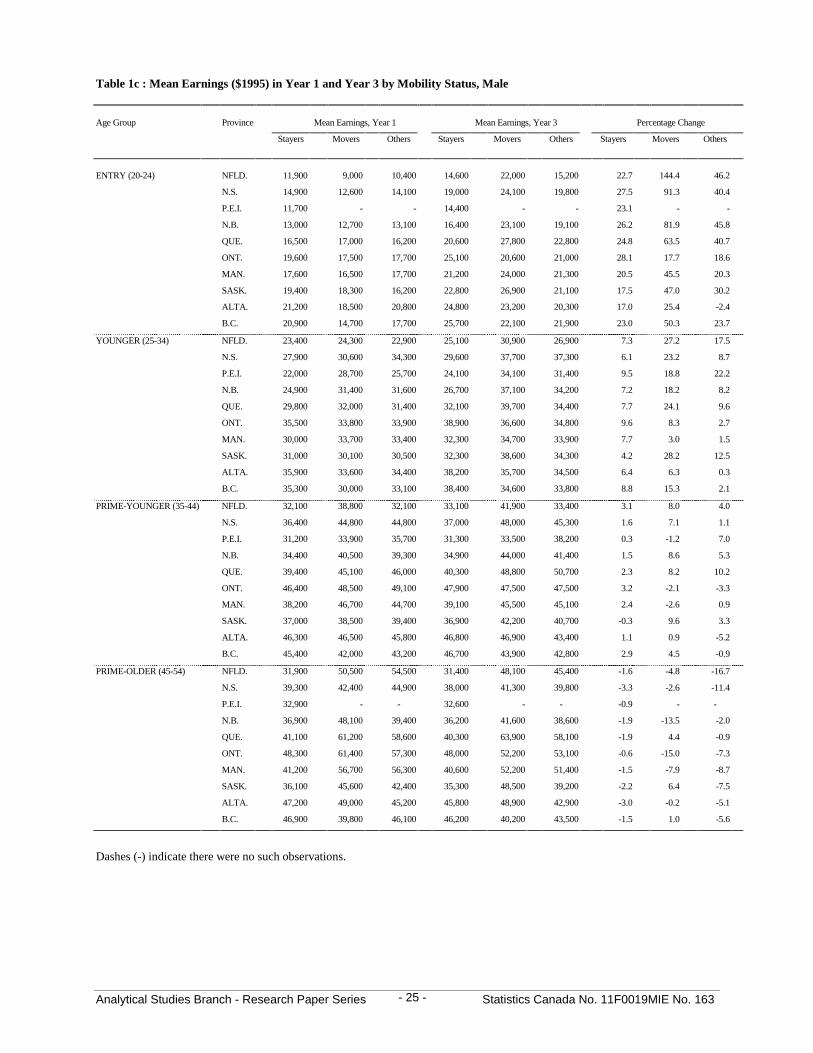
Analytical Studies Branch - Research Paper Series Statistics Canada No. 11F0019MIE No. 163- 25 -
Table 1c : Mean Earnings ($1995) in Year 1 and Year 3 by Mobility Status, Male
Age Group Province Mean Earnings, Year 1 Mean Earnings, Year 3 Percentage Change
Stayers Movers Others Stayers Movers Others Stayers Movers Others
ENTRY (20-24) NFLD. 11,900 9,000 10,400 14,600 22,000 15,200 22.7 144.4 46.2
N.S. 14,900 12,600 14,100 19,000 24,100 19,800 27.5 91.3 40.4
P.E.I. 11,700 - - 14,400 - - 23.1 - -
N.B. 13,000 12,700 13,100 16,400 23,100 19,100 26.2 81.9 45.8
QUE. 16,500 17,000 16,200 20,600 27,800 22,800 24.8 63.5 40.7
ONT. 19,600 17,500 17,700 25,100 20,600 21,000 28.1 17.7 18.6
MAN. 17,600 16,500 17,700 21,200 24,000 21,300 20.5 45.5 20.3
SASK. 19,400 18,300 16,200 22,800 26,900 21,100 17.5 47.0 30.2
ALTA. 21,200 18,500 20,800 24,800 23,200 20,300 17.0 25.4 -2.4
B.C. 20,900 14,700 17,700 25,700 22,100 21,900 23.0 50.3 23.7
YOUNGER (25-34) NFLD. 23,400 24,300 22,900 25,100 30,900 26,900 7.3 27.2 17.5
N.S. 27,900 30,600 34,300 29,600 37,700 37,300 6.1 23.2 8.7
P.E.I. 22,000 28,700 25,700 24,100 34,100 31,400 9.5 18.8 22.2
N.B. 24,900 31,400 31,600 26,700 37,100 34,200 7.2 18.2 8.2
QUE. 29,800 32,000 31,400 32,100 39,700 34,400 7.7 24.1 9.6
ONT. 35,500 33,800 33,900 38,900 36,600 34,800 9.6 8.3 2.7
MAN. 30,000 33,700 33,400 32,300 34,700 33,900 7.7 3.0 1.5
SASK. 31,000 30,100 30,500 32,300 38,600 34,300 4.2 28.2 12.5
ALTA. 35,900 33,600 34,400 38,200 35,700 34,500 6.4 6.3 0.3
B.C. 35,300 30,000 33,100 38,400 34,600 33,800 8.8 15.3 2.1
PRIME-YOUNGER (35-44) NFLD. 32,100 38,800 32,100 33,100 41,900 33,400 3.1 8.0 4.0
N.S. 36,400 44,800 44,800 37,000 48,000 45,300 1.6 7.1 1.1
P.E.I. 31,200 33,900 35,700 31,300 33,500 38,200 0.3 -1.2 7.0
N.B. 34,400 40,500 39,300 34,900 44,000 41,400 1.5 8.6 5.3
QUE. 39,400 45,100 46,000 40,300 48,800 50,700 2.3 8.2 10.2
ONT. 46,400 48,500 49,100 47,900 47,500 47,500 3.2 -2.1 -3.3
MAN. 38,200 46,700 44,700 39,100 45,500 45,100 2.4 -2.6 0.9
SASK. 37,000 38,500 39,400 36,900 42,200 40,700 -0.3 9.6 3.3
ALTA. 46,300 46,500 45,800 46,800 46,900 43,400 1.1 0.9 -5.2
B.C. 45,400 42,000 43,200 46,700 43,900 42,800 2.9 4.5 -0.9
PRIME-OLDER (45-54) NFLD. 31,900 50,500 54,500 31,400 48,100 45,400 -1.6 -4.8 -16.7
N.S. 39,300 42,400 44,900 38,000 41,300 39,800 -3.3 -2.6 -11.4
P.E.I. 32,900 - - 32,600 - - -0.9 - -
N.B. 36,900 48,100 39,400 36,200 41,600 38,600 -1.9 -13.5 -2.0
QUE. 41,100 61,200 58,600 40,300 63,900 58,100 -1.9 4.4 -0.9
ONT. 48,300 61,400 57,300 48,000 52,200 53,100 -0.6 -15.0 -7.3
MAN. 41,200 56,700 56,300 40,600 52,200 51,400 -1.5 -7.9 -8.7
SASK. 36,100 45,600 42,400 35,300 48,500 39,200 -2.2 6.4 -7.5
ALTA. 47,200 49,000 45,200 45,800 48,900 42,900 -3.0 -0.2 -5.1
B.C. 46,900 39,800 46,100 46,200 40,200 43,500 -1.5 1.0 -5.6
Dashes (-) indicate there were no such observations.

Analytical Studies Branch - Research Paper Series Statistics Canada No. 11F0019MIE No. 163- 26 -
Table 1c : Mean Earnings ($1995) in Year 1 and Year 3 by Mobility Status, Female
Age Group Province Mean Earnings, Year 1 Mean Earnings, Year 3 Percentage Change
Stayers Movers Others Stayers Movers Others Stayers Movers Others
ENTRY (20-24) NFLD. 11,100 10,900 11,000 13,400 17,900 11,900 20.7 64.2 8.2
N.S. 12,000 11,300 9,800 14,500 17,800 12,700 20.8 57.5 29.6
P.E.I. 11,100 8,000 8,600 13,100 11,500 9,500 18.0 43.8 10.5
N.B. 11,300 10,800 11,400 13,300 17,500 14,100 17.7 62.0 23.7
QUE. 13,600 13,700 12,800 16,100 19,600 16,500 18.4 43.1 28.9
ONT. 15,600 13,900 14,300 19,000 16,500 14,800 21.8 18.7 3.5
MAN. 14,300 15,400 14,800 16,800 19,000 15,400 17.5 23.4 4.1
SASK. 15,000 12,900 11,400 16,800 17,300 14,600 12.0 34.1 28.1
ALTA. 16,500 13,800 14,300 18,700 15,700 13,600 13.3 13.8 -4.9
B.C. 15,200 13,600 13,600 18,100 17,100 13,300 19.1 25.7 -2.2
YOUNGER(25-34)
NFLD. 16,700 16,800 15,700 17,700 18,400 15,300 6.0 9.5 -2.5
N.S. 18,100 20,000 20,000 19,300 21,800 19,200 6.6 9.0 -4.0
P.E.I. 15,400 15,900 19,800 16,400 16,500 14,500 6.5 3.8 -26.8
N.B. 16,600 21,600 17,500 17,800 23,600 16,600 7.2 9.3 -5.1
QUE. 20,800 22,700 21,200 22,000 25,300 21,800 5.8 11.5 2.8
ONT. 23,100 22,800 22,700 25,000 21,600 19,900 8.2 -5.3 -12.3
MAN. 20,200 21,000 21,300 21,500 18,700 18,200 6.4 -11.0 -14.6
SASK. 20,200 18,800 20,000 21,200 20,200 18,300 5.0 7.4 -8.5
ALTA. 22,800 21,300 21,000 23,700 19,200 17,500 3.9 -9.9 -16.7
B.C. 21,500 20,200 20,600 23,100 21,700 17,000 7.4 7.4 -17.5
PRIME-YOUNGER(35-44)
NFLD. 17,800 14,500 15,000 18,800 16,800 14,300 5.6 15.9 -4.7
N.S. 20,800 19,800 14,800 21,900 24,700 14,800 5.3 24.7 0.0
P.E.I. 18,700 - - 20,300 - - 8.6 - -
N.B. 19,500 22,100 21,300 20,600 22,500 17,300 5.6 1.8 -18.8
QUE. 23,700 23,900 22,600 24,800 23,300 19,800 4.6 -2.5 -12.4
ONT. 25,800 24,300 25,400 27,700 22,200 22,800 7.4 -8.6 -10.2
MAN. 22,900 19,600 19,900 24,500 16,300 16,200 7.0 -16.8 -18.6
SASK. 20,600 19,200 18,600 21,700 23,100 16,600 5.3 20.3 -10.8
ALTA. 24,600 20,900 20,000 25,800 18,200 17,900 4.9 -12.9 -10.5
B.C. 25,100 21,000 19,400 27,200 22,200 16,800 8.4 5.7 -13.4
PRIME-OLDER (45-54)
NFLD. 17,400 - - 16,900 - - -2.9 - -
N.S. 21,000 - - 20,900 - - -0.5 - -
P.E.I. 17,400 - - 16,900 - - -2.9 - -
N.B. 19,200 - - 19,000 - - -1.0 - -
QUE. 23,100 20,600 24,800 23,100 23,300 22,600 0.0 13.1 -8.9
ONT. 25,900 25,500 19,500 26,500 20,200 15,700 2.3 -20.8 -19.5
MAN. 22,500 23,600 21,200 22,700 18,800 16,000 0.9 -20.3 -24.5
SASK. 20,600 27,200 20,400 20,600 21,400 16,400 0.0 -21.3 -19.6
ALTA. 24,200 21,000 23,500 24,200 17,100 15,800 0.0 -18.6 -32.8
B.C. 25,200 23,100 23,600 25,800 22,300 17,900 2.4 -3.5 -24.2
Dashes (-) indicates there were no such observations.

Analytical Studies Branch - Research Paper Series Statistics Canada No. 11F0019MIE No. 163- 27 -
Table 2a : Level Equations, Male
Entry Younger Prime-Younger Prime -Older
(20-24) (25-34) (35-44) (45-54)
Intercept 2.642 ** (.922) 8.002 ** (.211) 8.337 ** (.406) 5.662 ** (.849)
Province (ONT)
NFLD. -.638 ** (.023) -.601 ** (.013) -.521 ** (.014) -.606 ** (.019)
N.S. -.297 ** (.017) -.300 ** (.010) -.296 ** (.011) -.234 ** (.015)
P.E.I. -.561 ** (.046) -.563 ** (.027) -.560 ** (.028) -.496 ** (.037)
N.B. -.439 ** (.020) -.442 ** (.012) -.340 ** (.012) -.338 ** (.017)
QUE. -.188 ** (.008) -.207 ** (.005) -.179 ** (.005) -.190 ** (.007)
MAN. -.158 ** (.017) -.193 ** (.009) -.199 ** (.010) -.175 ** (.013)
SASK. -.094 ** (.018) -.226 ** (.010) -.318 ** (.011) -.406 ** (.015)
ALTA. -.011 (.012) -.026 ** (.006) -.046 ** (.007) -.091 ** (.010)
B.C. .026 * (.012) -.007 (.006) -.022 ** (.006) -.039 ** (.008)
Mobility Status (stayers)
NFLD/Movers .628 ** (.097) .423 ** (.082) .353 ** (.130) .673 ** (.200)
NS/Movers .364 ** (.077) .261 ** (.056) .232 ** (.076) .156 (.169)
PEI/Movers .740 ** (.286) .575 ** (.178) .598 ** (.210) .840 (.447)
NB/Movers .290 ** (.098) .458 ** (.067) .105 (.097) -.051 (.192)
QUE/Movers .380 ** (.088) .262 ** (.072) -.100 (.099) .398 (.205)
ONT/Movers -.279 ** (.048) -.159 ** (.030) -.168 ** (.044) -.199 ** (.077)
MAN/Movers .152 (.082) .064 (.049) .146 * (.072) .233 * (.116)
SASK/Movers .163 * (.076) .225 ** (.053) .157 (.084) .300 * (.126)
ALTA/Movers -.158 ** (.052) -.154 ** (.031) -.021 (.047) .011 (.082)
BC/Movers -.182 ** (.061) -.141 ** (.041) -.157 ** (.057) -.229 * (.109)
Maritime/Returners -.158 (.107) -.279 ** (.102) -.137 (.156) .272 (.282)
QUE/Returners .410 * (.200) -.297 (.177) -.208 (.255) .050 (.446)
ONT/Returners -.551 ** (.113) -.402 ** (.083) -.482 ** (.133) -.047 (.195)
MAN/Returners -.093 (.185) -.465 * (.186) -.330 (.202) -.212 (.364)
SASK/Returners .033 (.195) -.326 * (.155) -.361 (.243) .796 (.515)
ALTA/Returners -.373 ** (.120) -.481 ** (.107) -.514 ** (.138) .061 (.297)
BC/Returners -.075 (.150) -.478 ** (.102) -.513 ** (.172) -.452 * (.230)
Min. Language (ENG/FR)
English-Quebec -.063 ** (.021) .042 ** (.012) .098 ** (.012) .111 ** (.015)
French-ROC -.062 * (.031) -.060 ** (.019) -.147 ** (.022) -.236 ** (.031)
Eng-Que/Movers -.099 (.131) -.102 (.092) .369 ** (.128) -.087 (.244)
Fr-ROC/Movers .333 ** (.122) .152 * (.078) .155 (.130) .117 (.248)
Eng-Que/Returners -.460 (.346) -.288 (.288) -1.112 ** (.416) .281 (.772)
Fr-ROC/Returners .535 (.604) .514 * (.272) -.408 (.477) -.386 (.913)
Personal Characteristics(single, no children) Married, no children .257 ** (.010) .267 ** (.005) .232 ** (.008) .226 ** (.010)
Married with children .009 (.002) .196 ** (.004) .309 ** (.006) .326 ** (.008)
Lone parent -.101 ** (.013) -.071 ** (.010) .044 ** (.006) .124 ** (.016)
Age .550 ** (.084) .118 ** (.014) .094 ** (.021) .204 ** (.034)
Age squared -.0100 ** (.0019) -.0014 ** (.0002) -.0011 ** (.0002) -.0021 ** (.0003)
Year (1984)
1985 -.001 (.014) .005 (.009) .024 * (.010) .014 (.013)
1986 .003 (.014) -.009 (.009) .019 (.010) .029 * (.013)
1987 .014 (.014) .007 (.009) .040 ** (.010) .057 ** (.013)
1988 .010 (.014) .020 * (.009) .054 ** (.010) .082 ** (.013)
1989 .018 (.015) .007 (.009) .050 ** (.010) .083 ** (.013)
1990 -.009 (.014) -.031 ** (.009) .009 (.010) .061 ** (.013)
1991 -.147 ** (.015) -.124 ** (.009) -.048 ** (.010) .014 (.013)
1992 -.202 ** (.016) -.136 ** (.009) -.057 ** (.010) .008 (.013)
1993 -.213 ** (.016) -.137 ** (.009) -.069 ** (.010) -.001 (.012)
1994 -.175 ** (.016) -.100 ** (.009) -.038 ** (.009) .025 * (.012)
1995 -.201 ** (.016) -.120 ** (.009) -.046 ** (.009) .046 ** (.012)
Standard errors are shown in parentheses. One asterisk indicates that the coefficient is significantly different from zero at the .05 confidencelevel according to a two-tailed t-test, two asterisks indicates significance at the .01 level. The models also include indicators of "arrivers" and"transients".

Analytical Studies Branch - Research Paper Series Statistics Canada No. 11F0019MIE No. 163- 28 -
Table 2b : Level Equations, Female
Entry Younger Prime-Younger Prime-Older
(20-24) (25-34) (35-44) (45-54)
Intercept -.510 (1.043) 9.314 ** (.280) 6.772 ** (.525) 6.370 ** (1.083)
Province (ONT)
NFLD. -.473 ** (.025) -.426 ** (.018) -.541 ** (.018) -.578 ** (.025)
N.S. -.295 ** (.020) -.276 ** (.014) -.302 ** (.015) -.278 ** (.020)
P.E.I. -.341 ** (.048) -.425 ** (.034) -.328 ** (.036) -.485 ** (.049)
N.B. -.377 ** (.023) -.387 ** (.016) -.347 ** (.017) -.350 ** (.021)
QUE. -.209 ** (.010) -.136 ** (.006) -.139 ** (.007) -.200 ** (.009)
MAN. -.133 ** (.019) -.147 ** (.012) -.095 ** (.013) -.123 ** (.017)
SASK. -.148 ** (.021) -.152 ** (.013) -.227 ** (.014) -.258 ** (.018)
ALTA. -.042 ** (.013) -.072 ** (.008) -.057 ** (.009) -.075 ** (.012)
B.C. -.056 ** (.013) -.115 ** (.008) -.033 ** (.008) -.025 * (.011)
Mobility Status (stayers)
NFLD/Movers .593 ** (.122) .128 (.116) -.334 * (.168) .443 (.270)
NS/Movers .162 (.087) -.023 (.084) -.112 (.121) .143 (.257)
PEI/Movers -.056 (.219) -.071 (.189) -.093 (.261) .139 (.681)
NB/Movers .200 (.135) .048 (.108) .082 (.159) -.362 (.290)
QUE/Movers .021 (.108) .035 (.105) -.332 * (.134) .186 (.430)
ONT/Movers -.293 ** (.056) -.306 ** (.046) -.557 ** (.067) -.560 ** (.105)
MAN/Movers .064 (.087) -.370 ** (.073) -.559 ** (.095) -.503 ** (.168)
SASK/Movers .009 (.086) -.284 ** (.081) -.127 (.105) -.489 * (.210)
ALTA/Movers -.210 ** (.060) -.317 ** (.045) -.492 ** (.070) -.351 ** (.119)
BC/Movers -.073 (.068) -.132 * (.062) -.379 ** (.085) -.379 * (.165)
Maritime/Returners -.261 (.141) -.357 * (.145) -.738 ** (.203) -.539 (.430)
QUE/Returners -.254 (.208) -.060 (.300) -.886 ** (.294) .239 (.960)
ONT/Returners -.505 ** (.147) -.661 ** (.134) -.507 ** (.176) -.764 * (.304)
MAN/Returners -.479 (.252) -.370 (.230) -1.548 ** (.417) -.606 (.679)
SASK/Returners -.599 * (.235) -.312 (.237) -.683 * (.380) -1.017 * (.481)
ALTA/Returners -.392 ** (.137) -.582 ** (.144) -.396 * (.208) -1.087 ** (.304)
BC/Returners -.547 ** (.159) -.761 ** (.159) -.937 ** (.203) -.514 ** (.430)
Min. Language (ENG/FR)
English-Quebec .175 ** (.022) .050 ** (.015) .077 ** (.015) .170 ** (.018)
French-ROC .025 (.038) -.012 (.025) -.032 (.027) .033 (.036)
Eng-Que/Mover .073 (.153) -.105 (.135) .150 (.176) -.507 (.467)
Fr-ROC/Mover .274 * (.153) .234 ** (.114) .338 * (.170) -1.549 ** (.442)
Eng-Que/Returner .107 (.426) -.470 (.424) .342 (.459) 1.143 (1.358)
Fr-ROC/Returner .232 (.419) .579 (.480) -1.406 (.948) 1.257 (1.008)
Personal Characteristics (single,no children) Married, no children -.081 ** (.010) -.080 ** (.007) -.122 ** (.011) -.215 ** (.011)
Married with children -.168 ** (.008) -.432 ** (.006) -.342 ** (.008) -.251 ** (.010)
Lone parent -.294 ** (.014) -.392 ** (.010) -.221 ** (.010) -.086 ** (.013)
Age .838 ** (.095) .025 (.019) .167 ** (.027) .171 ** (.044)
Age squared -.0169 ** (.0021) .0001 (.0003) -.0021 ** (.0003) -.0020 ** (.0004)
Year (1984)
1985 -.030 (.016) .008 (.012) .023 (.014) .015 (.018)
1986 -.034 * (.016) -.011 (.012) .052 ** (.014) .024 (.018)
1987 -.017 (.016) .006 (.012) .070 ** (.013) .044 * (.017)
1988 -.033 * (.016) .007 (.012) .110 ** (.013) .094 ** (.017)
1989 -.018 (.016) .001 (.012) .116 ** (.013) .099 ** (.017)
1990 -.005 (.016) .002 (.012) .143 ** (.013) .096 ** (.017)
1991 -.097 ** (.017) -.027 * (.012) .124 ** (.013) .078 ** (.017)
1992 -.152 ** (.018) -.041 ** (.012) .138 ** (.013) .108 ** (.016)
1993 -.157 ** (.018) -.039 ** (.012) .121 ** (.013) .121 ** (.016)
1994 -.149 ** (.018) -.018 (.012) .150 ** (.013) .150 ** (.016)
1995 -.222 ** (.018) -.027 * (.012) .152 ** (.013) .170 ** (.016)
Standard errors are shown in parentheses. One asterisk indicates that the coefficient is significantly different from zero at the .05 confidence level according to atwo-tailed t-test, two asterisks indicates significance at the .01 level. The models also include indicators of "arrivers" and "transients".

Analytical Studies Branch - Research Paper Series Statistics Canada No. 11F0019MIE No. 163- 29 -
Table 3a : Fixed Effects, Male
Entry Younger Prime-Younger Prime-Older
(20-24) (25-34) (35-44) (45-54)
Intercept 2.371 * (.948) 1.592 ** (.188) .130 (.321) -2.167 ** (.649)
Province (ONT)
NFLD. -.102 ** (.023) -.012 (.012) -.001 (.011) -.021 (.015)
N.S. -.012 (.018) -.023 * (.009) -.018 * (.009) -.043 ** (.011)
P.E.I. -.072 (.048) .014 (.024) -.047 * (.022) .012 (.028)
N.B. -.024 (.020) -.016 (.010) -.010 (.010) -.014 (.013)
QUE. -.027 ** (.009) -.018 ** (.004) -.008 * (.004) -.020 ** (.005)
MAN. -.083 ** (.017) -.009 (.008) -.006 (.008) -.010 (.010)
SASK. -.119 ** (.018) -.045 ** (.009) -.044 ** (.009) -.039 ** (.011)
ALTA. -.108 ** (.012) -.026 ** (.006) -.021 ** (.005) -.022 ** (.007)
B.C. -.021 (.012) .010 (.006) .001 (.005) .002 (.006)
Mobility Status (stayers)
NFLD/Movers .883 ** (.100) .371 ** (.072) .383 ** (.102) .092 (.153)
NS/Movers .545 ** (.079) .137 ** (.050) .079 (.060) .014 (.129)
PEI/Movers .504 (.294) .323 * (.159) -.038 (.166) .282 (.342)
NB/Movers .466 ** (.101) .181 ** (.060) .023 (.076) -.270 (.147)
QUE/Movers .439 ** (.091) .283 ** (.064) .067 (.078) -.073 (.145)
ONT/Movers -.150 ** (.049) -.025 (.027) -.187 ** (.035) -.349 ** (.059)
MAN/Movers .347 ** (.084) -.041 (.043) -.053 (.057) -.085 (.088)
SASK/Movers .288 ** (.078) .236 ** (.047) .148 * (.067) .191 * (.096)
ALTA/Movers .030 (.054) -.046 (.027) .011 (.037) -.058 (.063)
BC/Movers .159 * (.062) .112 ** (.036) .089 * (.045) .024 (.083)
Maritime/Returners .068 (.110) -.170 (.091) .151 (.123) .221 (.216)
QUE/Returners .033 (.205) -.059 (.157) -.175 (.201) -.432 (.341)
ONT/Returners -.263 * (.116) -.076 (.074) -.269 * (.105) -.001 (.149)
MAN/Returners .136 (.190) -.262 (.166) .235 (.159) -.759 ** (.278)
SASK/Returners .000 (.200) .107 (.138) -.103 (.192) .494 (.393)
ALTA/Returners -.220 (.123) -.156 (.095) -.213 (.109) .007 (.227)
BC/Returners .025 (.154) -.004 (.091) -.002 (.136) .274 (.176)
Min. Language (ENG/FR)
English-Quebec -.017 (.021) .035 ** (.010) .009 (.009) .007 (.012)
French-ROC -.009 (.032) .013 (.017) -.015 (.017) -.016 (.024)
Eng-Que/Movers -.179 (.135) -.101 (.082) .009 (.101) -.137 (.190)
Fr-ROC/Movers .093 (.125) .030 (.069) -.105 (.103) -.033 (.196)
Eng-Que/Returners .061 (.335) -.472 * (.256) -.210 (.329) .115 (.590)
Fr-ROC/Returners 2.403 ** (.621) .368 (.242) -.123 (.377) -1.642 * (.697)
Personal Characteristics(single, no children) Married, no children -.034 ** (.010) .003 (.005) .011 * (.006) .001 (.007)
Married with children .037 ** (.007) -.026 ** (.004) -.004 (.004) .018 ** (.006)
Lone parent .020 (.013) -.034 ** (.009) -.024 ** (.009) -.011 (.012)
Age -.152 * (.086) -.091 ** (.013) -.001 (.016) .098 ** (.026)
Age squared .0025 (.0020) .0013 ** (.0002) -.0001 (.0002) -.0014 ** (.0003)
Year (1984)
1985 .083 ** (.015) .053 ** (.008) .035 ** (.008) .031 ** (.010)
1986 .076 ** (.015) .024 ** (.008) .017 * (.008) .033 ** (.010)
1987 .100 ** (.015) .034 ** (.008) .014 (.008) .038 ** (.010)
1988 .125 ** (.015) .061 ** (.008) .040 ** (.008) .055 ** (.010)
1989 .087 ** (.015) .044 ** (.008) .016 * (.008) .023 * (.010)
1990 .016 (.015) -.018 * (.008) -.046 ** (.008) -.029 ** (.010)
1991 -.179 ** (.016) -.119 ** (.008) -.108 ** (.008) -.093 ** (.010)
1992 -.175 ** (.016) -.115 ** (.008) -.084 ** (.008) -.092 ** (.010)
1993 -.042 * (.016) -.031 ** (.008) -.039 ** (.008) -.046 ** (.010)
1994 .082 ** (.017) .047 ** (.008) .014 (.007) -.004 (.009)
1995 .119 ** (.017) .056 ** (.008) .035 ** (.007) .034 ** (.009)
Standard errors are shown in parentheses. One asterisk indicates that the coefficient is significantly different from zero at the .05 confidence levelaccording to a two-tailed t-test, two asterisks indicates significance at the .01 level. The models also include indicators of "arrivers" and "transients".
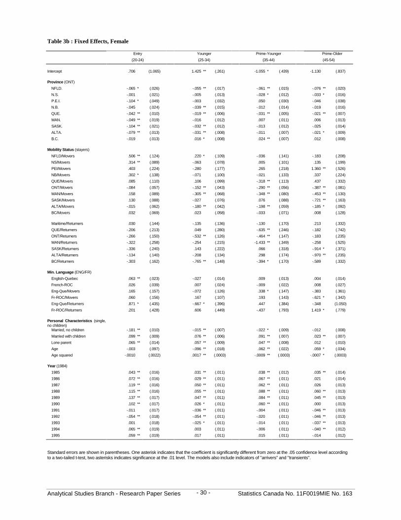
Analytical Studies Branch - Research Paper Series Statistics Canada No. 11F0019MIE No. 163- 30 -
Table 3b : Fixed Effects, Female
Entry Younger Prime-Younger Prime-Older
(20-24) (25-34) (35-44) (45-54)
Intercept .706 (1.065) 1.425 ** (.261) -1.055 * (.439) -1.130 (.837)
Province (ONT)
NFLD. -.065 * (.026) -.055 ** (.017) -.061 ** (.015) -.076 ** (.020)
N.S. -.001 (.021) -.005 (.013) -.028 * (.012) -.033 * (.016)
P.E.I. -.104 * (.049) -.003 (.032) .050 (.030) -.046 (.038)
N.B. -.045 (.024) -.039 ** (.015) -.012 (.014) -.019 (.016)
QUE. -.042 ** (.010) -.019 ** (.006) -.031 ** (.005) -.021 ** (.007)
MAN. -.049 ** (.019) -.016 (.012) .007 (.011) .006 (.013)
SASK. -.104 ** (.021) -.032 ** (.012) -.013 (.012) -.025 (.014)
ALTA. -.079 ** (.013) -.031 ** (.008) -.011 (.007) -.021 * (.009)
B.C. -.019 (.013) .016 * (.008) .024 ** (.007) .012 (.008)
Mobility Status (stayers)
NFLD/Movers .506 ** (.124) .220 * (.109) -.036 (.141) -.183 (.208)
NS/Movers .314 ** (.089) -.063 (.078) .005 (.101) .135 (.199)
PEI/Movers .403 (.224) -.280 (.177) .265 (.218) 1.360 ** (.526)
NB/Movers .302 * (.138) -.071 (.100) -.021 (.133) .337 (.224)
QUE/Movers .085 (.110) .106 (.099) -.318 ** (.113) .437 (.332)
ONT/Movers -.084 (.057) -.152 ** (.043) -.290 ** (.056) -.387 ** (.081)
MAN/Movers .158 (.089) -.305 ** (.068) -.348 ** (.080) -.453 ** (.130)
SASK/Movers .130 (.088) -.027 (.076) .076 (.088) -.721 ** (.163)
ALTA/Movers -.015 (.062) -.180 ** (.042) -.198 ** (.059) -.185 * (.092)
BC/Movers .032 (.069) .023 (.058) -.033 (.071) .008 (.128)
Maritime/Returners .030 (.144) -.135 (.136) -.130 (.170) .213 (.332)
QUE/Returners -.206 (.213) .049 (.280) -.635 ** (.246) -.182 (.742)
ONT/Returners -.266 (.150) -.532 ** (.126) -.464 ** (.147) -.183 (.235)
MAN/Returners -.322 (.258) -.254 (.215) -1.433 ** (.349) -.258 (.525)
SASK/Returners -.336 (.240) .143 (.222) .066 (.318) -.914 * (.371)
ALTA/Returners -.134 (.140) -.208 (.134) .298 (.174) -.970 ** (.235)
BC/Returners -.303 (.162) -.765 ** (.148) -.394 * (.170) -.589 (.332)
Min. Language (ENG/FR)
English-Quebec .063 ** (.023) -.027 (.014) .009 (.013) .004 (.014)
French-ROC .026 (.039) .007 (.024) -.009 (.022) .008 (.027)
Eng-Que/Movers .165 (.157) -.072 (.126) .338 * (.147) -.383 (.361)
Fr-ROC/Movers .060 (.156) .167 (.107) .193 (.143) -.621 * (.342)
Eng-Que/Returners .871 * (.435) -.667 * (.396) .447 (.384) -.348 (1.050)
Fr-ROC/Returners .201 (.428) .606 (.449) -.437 (.793) 1.419 * (.779)
Personal Characteristics (single,no children) Married, no children -.181 ** (.010) -.015 ** (.007) -.022 * (.009) -.012 (.008)
Married with children .099 ** (.009) .076 ** (.006) .091 ** (.007) .023 ** (.007)
Lone parent .065 ** (.014) .057 ** (.009) .047 ** (.008) .012 (.010)
Age -.003 (.097) -.096 ** (.018) .062 ** (.022) .059 * (.034)
Age squared -.0010 (.0022) .0017 ** (.0003) -.0009 ** (.0003) -.0007 * (.0003)
Year (1984)
1985 .043 ** (.016) .031 ** (.011) .038 ** (.012) .035 ** (.014)
1986 .072 ** (.016) .029 ** (.011) .067 ** (.011) .021 (.014)
1987 .119 ** (.016) .050 ** (.011) .062 ** (.011) .026 (.013)
1988 .115 ** (.016) .055 ** (.011) .088 ** (.011) .060 ** (.013)
1989 .137 ** (.017) .047 ** (.011) .084 ** (.011) .045 ** (.013)
1990 .102 ** (.017) .026 * (.011) .060 ** (.011) .000 (.013)
1991 -.011 (.017) -.036 ** (.011) -.004 (.011) -.046 ** (.013)
1992 -.054 ** (.018) -.054 ** (.011) -.020 (.011) -.046 ** (.013)
1993 .001 (.018) -.025 * (.011) -.014 (.011) -.037 ** (.013)
1994 .065 ** (.019) .003 (.011) -.006 (.011) -.040 ** (.012)
1995 .059 ** (.019) .017 (.011) .015 (.011) -.014 (.012)
Standard errors are shown in parentheses. One asterisk indicates that the coefficient is significantly different from zero at the .05 confidence level accordingto a two-tailed t-test, two asterisks indicates significance at the .01 level. The models also include indicators of "arrivers" and "transients".

Analytical Studies Branch - Research Paper Series Statistics Canada No. 11F0019MIE No. 163- 31 -
Table 4a : Pre-Move Earnings Profiles, Male
Entry Younger Prime-Younger Prime-Older
(20-24) (25-34) (35-44) (45-54)
Intercept 3.126 ** (1.031) 1.461 ** (.196) -.234 (.334) -.045 (.649)
Province (ONT)
NFLD. -.083 ** (.025) -.038 ** (.012) -.010 (.012) -.029 * (.015)
N.S. -.010 (.019) -.031 ** (.009) -.016 (.009) -.029 * (.011)
P.E.I. -.060 (.051) -.011 (.024) -.055 * (.023) -.017 (.028)
N.B. -.048 * (.022) -.027 * (.011) -.019 (.010) -.017 (.013)
QUE. -.031 ** (.009) -.021 ** (.004) -.015 ** (.004) -.016 ** (.005)
MAN. -.082 ** (.018) -.026 ** (.009) -.018 * (.008) -.027 ** (.010)
SASK. -.159 ** (.019) -.066 ** (.009) -.049 ** (.009) -.052 ** (.011)
ALTA. -.131 ** (.013) -.036 ** (.006) -.033 ** (.006) -.033 ** (.007)
B.C. -.015 (.014) .011 (.006) -.001 (.005) -.003 (.006)
Mobility Status (stayers)
NFLD/Pre-Move -.093 (.158) .004 (.100) -.106 (.148) .053 (.175)
NS/Pre-Move -.237 * (.103) .021 (.068) -.073 (.079) -.133 (.155)
PEI/Pre-Move -.716 (.410) -.192 (.242) .084 (.234) -.022 (.580)
NB/Pre-Move .106 (.141) .059 (.080) -.052 (.094) -.027 (.161)
QUE/Pre-Move -.016 (.096) -.009 (.054) -.109 (.061) -.307 ** (.101)
ONT/Pre-Move -.062 (.072) -.073 * (.033) -.015 (.044) -.019 (.072)
MAN/Pre-Move -.214 * (.108) .085 (.057) -.003 (.070) -.018 (.104)
SASK/Pre-Move -.001 (.114) .011 (.062) -.019 (.080) -.371 ** (.119)
ALTA/Pre-Move -.130 (.081) -.043 (.036) -.045 (.046) .049 (.078)
BC/Pre-Move -.008 (.100) -.129 * (.050) .008 (.068) -.188 (.110)
NFLD/Movers .684 ** (.108) .397 ** (.079) .064 (.105) .040 (.146)
NS/Movers .519 ** (.092) .169 ** (.052) .144 * (.062) -.139 (.130)
PEI/Movers .784 (.411) .507 ** (.166) -.059 (.154) .284 (.291)
NB/Movers .534 ** (.105) .142 * (.062) .056 (.080) -.003 (.156)
QUE/Movers .551 ** (.095) .269 ** (.064) .041 (.089) .187 (.155)
ONT/Movers -.175 ** (.056) -.078 ** (.029) -.149 ** (.037) -.328 ** (.061)
MAN/Movers .317 ** (.096) -.040 (.046) -.059 (.056) -.013 (.094)
SASK/Movers .279 ** (.083) .246 ** (.048) .076 (.068) .308 ** (.096)
ALTA/Movers .071 (.059) -.048 (.028) .048 (.039) -.065 (.062)
BC/Movers .174 * (.070) .108 ** (.039) .082 (.047) .096 (.085)
Maritime/Returners .098 (.128) -.155 (.102) .163 (.139) .238 (.219)
QUE/Returners .120 (.217) .230 (.170) .188 (.216) .047 (.334)
ONT/Returners -.339 * (.138) -.049 (.080) -.242 * (.116) -.160 (.155)
MAN/Returners -.047 (.211) -.376 (.212) .179 (.158) -.170 (.335)
SASK/Returners .052 (.258) .195 (.150) -.172 (.190) .111 (.410)
ALTA/Returners -.341 * (.140) -.061 (.106) -.275 * (.110) .056 (.219)
BC/Returners -.084 (.174) -.109 (.101) -.129 (.143) .473 ** (.175)
Min. Language (ENG/FR)
English-Quebec -.022 (.024) .045 ** (.011) .014 (.010) .006 (.012)
French-ROC -.027 (.034) .001 (.017) -.014 (.018) -.034 (.024)
Eng-Que/Movers -.230 (.145) -.134 (.084) .000 (.113) -.045 (.183)
Fr-ROC/Movers .010 (.139) .132 (.071) -.061 (.135) -.021 (.191)
Eng-Que/Returners .157 (.377) -.518 (.361) -.173 (.394) -.394 (.529)
Fr-ROC/Returners .192 (.824) .196 (.274) .443 (.587) -1.497 * (.600)
Personal Characteristics (single,no children) Married, no children -.054 ** (.011) -.004 (.005) .004 (.007) -.006 (.008)
Married with children .020 * (.008) -.037 ** (.004) -.017 ** (.005) -.004 (.007)
Lone parent .013 (.014) -.035 ** (.009) -.028 ** (.010) -.003 (.013)
Age -.216 * (.094) -.081 ** (.013) .019 (.017) .009 (.026)
Age squared .0040 (.0021) .0012 ** (.0002) -.0003 (.0002) -.0002 (.0003)
Standard errors are shown in parentheses. One asterisk indicates that the coefficient is significantly different from zero at the .05 confidence levelaccording to a two-tailed t-test, two asterisks indicates significance at the .01 level. The models also include indicators of "arrivers" and "transients".

Analytical Studies Branch - Research Paper Series Statistics Canada No. 11F0019MIE No. 163- 32 -
Table 4b : Pre-Move Earnings Profiles, Female
Entry Younger Prime-Younger Prime-Older
(20-24) (25-34) (35-44) (45-54)
Intercept 1.996 (1.132) 1.121 ** (.277) -.683 (.472) .042 (.855)
Province (ONT)
NFLD. -.104 ** (.028) -.063 ** (.018) -.079 ** (.016) -.043 * (.020)
N.S. .012 (.022) -.009 (.014) -.029 * (.013) -.033 * (.016)
P.E.I. -.138 ** (.051) -.039 (.034) .071 * (.032) -.018 (.038)
N.B. -.048 (.025) -.033 * (.016) -.024 (.015) -.037 * (.016)
QUE. -.025 * (.010) -.028 ** (.006) -.030 ** (.006) -.024 ** (.007)
MAN. -.036 (.020) -.031 * (.012) -.001 (.011) -.006 (.013)
SASK. -.135 ** (.023) -.051 ** (.013) -.012 (.013) -.066 ** (.014)
ALTA. -.082 ** (.014) -.038 ** (.008) -.028 ** (.008) -.030 ** (.010)
B.C. -.031 * (.015) .015 (.008) .016 * (.007) .004 (.009)
Mobility Status (stayers)
NFLD/Pre-Move .263 (.170) .148 (.171) .122 (.159) .137 (.362)
NS/Pre-Move -.084 (.128) -.014 (.110) .053 (.145) .039 (.314)
PEI/Pre-Move .256 (.379) -.032 (.268) -.261 (.501) - -
NB/Pre-Move -.012 (.199) .193 (.130) .066 (.214) -.167 (.443)
QUE/Pre-Move .126 (.102) .072 (.085) .003 (.097) .015 (.157)
ONT/Pre-Move .108 (.078) .046 (.054) .037 (.075) -.134 (.098)
MAN/Pre-Move -.107 (.117) .070 (.088) .147 (.105) -.222 (.157)
SASK/Pre-Move .125 (.114) .080 (.091) .068 (.109) .053 (.189)
ALTA/Pre-Move .086 (.088) -.009 (.054) -.115 (.083) -.025 (.103)
BC/Pre-Move .125 (.108) .039 (.081) .276 ** (.104) .273 (.198)
NFLD/Movers .306 * (.143) .216 (.119) .398 * (.167) -.173 (.203)
NS/Movers .324 ** (.097) .006 (.083) .044 (.111) .152 (.199)
PEI/Movers .347 (.248) -.282 (.182) .478 (.269) 1.194 (.628)
NB/Movers .595 ** (.151) -.217 * (.104) .071 (.140) .485 * (.222)
QUE/Movers .187 (.122) .364 ** (.105) -.546 ** (.115) .437 (.313)
ONT/Movers -.071 (.062) -.124 ** (.047) -.226 ** (.062) -.189 * (.082)
MAN/Movers .132 (.095) -.310 ** (.071) -.302 ** (.084) -.462 ** (.141)
SASK/Movers .095 (.094) -.011 (.082) .039 (.098) -.744 ** (.181)
ALTA/Movers -.031 (.067) -.169 ** (.045) -.076 (.064) -.161 (.095)
BC/Movers .152 * (.075) .004 (.059) -.108 (.078) -.063 (.131)
Maritime/Returners .025 (.162) -.109 (.142) -.089 (.189) .418 (.362)
QUE/Returners -.124 (.225) .039 (.326) -.692 * (.289) -.258 (.626)
ONT/Returners -.108 (.168) -.362 ** (.134) -.438 ** (.162) -.308 (.209)
MAN/Returners -.212 (.281) -.249 (.214) -1.693 ** (.408) -.389 (.627)
SASK/Returners -.080 (.281) .181 (.266) .012 (.354) -1.583 ** (.443)
ALTA/Returners -.093 (.157) -.099 (.141) .159 (.183) -1.164 ** (.313)
BC/Returners -.092 (.193) -.812 ** (.190) -.637 ** (.204) .068 (.362)
Min. Language (ENG/FR)
English-Quebec .054 * (.025) -.012 (.015) .007 (.013) .004 (.014)
French-ROC -.023 (.040) -.003 (.025) -.021 (.024) .027 (.028)
Eng-Que/Movers -.026 (.170) -.295 * (.132) .677 ** (.152) -.385 (.341)
Fr-ROC/Movers .019 (.151) .055 (.109) .087 (.162) -.236 (.373)
Eng-Que/Returners 1.233 ** (.477) -.803 (.444) .438 (.578) -.328 (.886)
Fr-ROC/Returners .035 (.858) .577 (.470) - - 1.457 * (.661)
Personal Characteristics (single, no children)
Married, no children -.155 ** (.011) -.115 ** (.007) -.016 (.010) .004 (.008)
Married with children .114 ** (.010) .103 ** (.006) .098 ** (.007) .031 ** (.008)
Lone parent .080 ** (.015) .090 ** (.009) .045 ** (.009) .016 (.011)
Age -.115 (.103) -.072 ** (.019) .044 (.024) .008 (.035)
Age squared .0015 (.0023) .0012 ** (.0003) -.0007 * (.0003) -.0002 (.0004)
Standard errors are shown in parentheses. One asterisk indicates that the coefficient is significantly different from zero at the .05 confidence levelaccording to a two-tailed t-test, two asterisks indicates significance at the .01 level. The models also include indicators of "arrivers" and "transients".
Dashes (-) indicate there were no such observations.
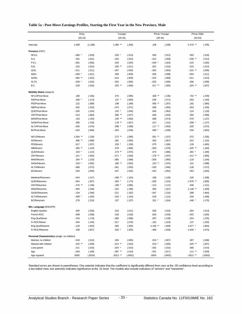
Analytical Studies Branch - Research Paper Series Statistics Canada No. 11F0019MIE No. 163- 33 -
Table 5a : Post-Move Earnings Profiles, Starting the First Year in the New Province, Male
Entry Younger Prime-Younger Prime-Older
(20-24) (25-34) (35-44) (45-54)
Intercept 1.008 (1.186) 1.480 ** (.206) .108 (.338) -2.470 ** (.705)
Province (ONT)
NFLD. -.066 * (.029) .026 * (.013) .005 (.012) .003 (.016)
N.S. .031 (.021) -.010 (.010) -.012 (.009) -.036 ** (.012)
P.E.I. -.052 (.056) .044 (.025) -.045 * (.023) .015 (.030)
N.B. .015 (.024) .030 ** (.011) .001 (.010) .010 (.014)
QUE. -.011 (.011) -.007 (.004) -.002 (.004) -.015 ** (.006)
MAN. -.049 * (.021) .006 (.009) .005 (.008) -.004 (.011)
SASK. -.082 ** (.022) -.014 (.009) -.015 (.009) -.011 (.013)
ALTA. -.039 * (.015) -.002 (.006) -.003 (.006) .006 (.008)
B.C. .018 (.016) .025 ** (.006) .017 ** (.005) .024 ** (.007)
Mobility Status (stayers)
NFLD/Post-Move .180 (.165) .075 (.090) .358 ** (.130) .702 ** (.249)
NS/Post-Move .266 * (.113) .137 * (.060) .039 (.071) .053 (.140)
PEI/Post-Move .122 (.368) .198 (.169) .956 ** (.297) .182 (.380)
NB/Post-Move .002 (.153) -.073 (.071) .096 (.094) .053 (.155)
QUE/Post-Move -.200 (.104) .102 * (.045) .060 (.063) .124 (.118)
ONT/Post-Move .013 (.060) .080 ** (.027) .000 (.033) .055 (.058)
MAN/Post-Move .153 (.150) .240 ** (.063) .089 (.073) .070 (.137)
SASK/Post-Move .090 (.150) .178 ** (.067) .012 (.101) -.296 * (.147)
ALTA/Post-Move -.030 (.076) .098 * (.038) .117 ** (.043) .020 (.075)
BC/Post-Move -.024 (.084) -.003 (.034) .099 * (.039) .034 (.063)
NFLD/Movers 1.054 ** (.126) .272 ** (.085) .561 ** (.107) .072 (.156)
NS/Movers .486 ** (.098) .081 (.055) .053 (.067) .012 (.132)
PEI/Movers .617 (.337) .333 * (.159) .075 (.180) .126 (.465)
NB/Movers .365 ** (.120) .079 (.069) -.053 (.079) -.425 ** (.160)
QUE/Movers .244 * (.114) .273 ** (.075) .074 (.085) .391 * (.190)
ONT/Movers -.141 * (.063) -.071 * (.030) -.178 ** (.037) -.412 ** (.065)
MAN/Movers .354 ** (.103) -.085 (.048) -.059 (.060) -.119 (.104)
SASK/Movers .233 * (.092) .180 ** (.052) .223 ** (.070) .101 (.098)
ALTA/Movers -.068 (.072) -.051 (.033) -.030 (.040) -.128 (.072)
BC/Movers .033 (.083) .047 (.042) -.022 (.052) .053 (.093)
Maritime/Returners -.044 (.147) -.408 ** (.104) .158 (.126) .220 (.208)
QUE/Returners -.054 (.307) -.363 * (.173) -.065 (.224) -1.976 ** (.656)
ONT/Returners -.476 ** (.146) -.189 * (.085) -.213 (.112) .046 (.151)
MAN/Returners -.050 (.246) -.252 (.196) .092 (.187) -1.148 ** (.328)
SASK/Returners -.134 (.246) -.221 (.162) -.047 (.210) .589 (.464)
ALTA/Returners -.358 * (.160) -.233 * (.104) .018 (.121) .034 (.248)
BC/Returners .278 (.210) .107 (.107) .331 * (.164) .446 * (.176)
Min. Language (ENG/FR)
English-Quebec .004 (.026) .015 (.011) .005 (.010) .004 (.013)
French-ROC .008 (.038) .018 (.018) .003 (.018) -.042 (.026)
Eng-Que/Mover -.194 (.179) -.085 (.098) .097 (.109) -.324 (.225)
Fr-ROC/Mover .044 (.144) -.017 (.076) -.162 (.103) .137 (.240)
Eng-Que/Returner -.129 (.453) .082 (.300) -1.196 ** (.409) 1.677 * (.804)
Fr-ROC/Returner .328 (.827) .520 * (.255) -.468 (.434) -1.640 * (.674)
Personal Characteristics (single, no children)
Married, no children -.018 (.013) .004 (.005) .015 * (.007) .007 (.008)
Married with children .042 ** (.009) -.012 ** (.004) .010 * (.005) .025 ** (.007)
Lone parent .011 (.016) -.024 * (.010) -.002 (.010) .000 (.014)
Age -.034 (.108) -.087 ** (.014) -.001 (.017) .111 ** (.029)
Age squared .0000 (.0024) .0013 ** (.0002) .0000 (.0002) -.0012 ** (.0003)
Standard errors are shown in parentheses. One asterisk indicates that the coefficient is significantly different from zero at the .05 confidence level according toa two-tailed t-test, two asterisks indicates significance at the .01 level. The models also include indicators of "arrivers" and "transients".

Analytical Studies Branch - Research Paper Series Statistics Canada No. 11F0019MIE No. 163- 34 -
Table 5b : Post-Move Earnings Profiles, Starting the First Year in the New Province, Female
Entry Younger Prime-Younger Prime-Older
(20-24) (25-34) (35-44) (45-54)
Intercept -.565 (1.397) 1.091 ** (.287) -.796 (.448) -1.020 (.885)
Province (ONT)
NFLD. -.029 (.033) .00005 (.018) -.027 (.016) -.071 ** (.021)
N.S. .028 (.026) .019 (.014) -.040 ** (.013) -.035 * (.017)
P.E.I. -.018 (.059) .024 (.034) .030 (.031) -.017 (.039)
N.B. -.008 (.029) -.011 (.016) -.022 (.015) -.005 (.017)
QUE. -.042 ** (.012) .001 (.006) -.025 ** (.006) -.019 ** (.007)
MAN. -.044 (.024) -.006 (.013) .005 (.011) .003 (.014)
SASK. -.080 ** (.027) -.017 (.013) -.013 (.012) -.013 (.015)
ALTA. -.067 ** (.017) -.026 ** (.009) -.011 (.008) -.017 (.010)
B.C. .025 (.017) .011 (.009) .028 ** (.007) .016 (.009)
Mobility Status (stayers)
NFLD/Post-Move .412 (.278) .117 (.158) .341 (.219) .390 (.400)
NS/Post-Move .199 (.131) .324 ** (.092) .373 ** (.104) .534 ** (.201)
PEI/Post-Move -.019 (.395) .571 * (.291) .003 (.263) .068 (.694)
NB/Post-Move .295 (.202) .349 ** (.116) .730 ** (.136) -.053 (.245)
QUE/Post-Move -.016 (.142) .209 ** (.071) .192 * (.085) -.193 (.209)
ONT/Post-Move .174 * (.072) .112 ** (.040) .165 ** (.047) .088 (.074)
MAN/Post-Move -.309 (.184) .173 (.098) .408 ** (.124) .184 (.200)
SASK/Post-Move -.018 (.157) .067 (.103) .323 * (.127) .237 (.231)
ALTA/Post-Move .068 (.079) .019 (.055) -.036 (.066) .251 * (.117)
BC/Post-Move .047 (.084) .129 * (.050) .300 ** (.056) .463 ** (.087)
NFLD/Movers .386 * (.174) .045 (.130) .124 (.159) -.275 (.213)
NS/Movers .302 ** (.117) -.136 (.087) -.103 (.107) .205 (.209)
PEI/Movers .353 (.270) -.253 (.182) .104 (.220) -
NB/Movers .336 (.183) -.120 (.110) -.202 (.155) .120 (.246)
QUE/Movers .174 (.142) .009 (.113) -.504 ** (.128) .323 (.400)
ONT/Movers -.181 * (.078) -.187 ** (.048) -.466 ** (.060) -.429 ** (.092)
MAN/Movers .282 * (.110) -.396 ** (.075) -.336 ** (.085) -.530 ** (.142)
SASK/Movers .237 * (.108) -.186 * (.084) .119 (.086) -.477 ** (.174)
ALTA/Movers .071 (.086) -.208 ** (.048) -.182 ** (.064) -.328 ** (.099)
BC/Movers .129 (.092) -.096 (.067) .003 (.077) -.063 (.151)
Maritime/Returners .096 (.184) -.326 * (.148) -.124 (.173) -.207 (.400)
QUE/Returners -.503 (.357) .020 (.309) -.749 ** (.261) -.504 (.693)
ONT/Returners -.550 * (.237) -.598 ** (.140) -.618 ** (.167) -.175 (.283)
MAN/Returners -.190 (.310) -.434 (.236) -1.438 ** (.345) -.225 (.490)
SASK/Returners -.468 (.278) -.179 (.259) .282 (.309) -1.298 ** (.490)
ALTA/Returners -.129 (.219) -.331 * (.155) .304 (.230) -1.410 ** (.310)
BC/Returners -.430 (.221) -.539 ** (.185) -.413 * (.185) .140 (.400)
Min. Language (ENG/FR)
English-Quebec .089 ** (.029) -.039 * (.015) .014 (.013) .002 (.015)
French-ROC .073 (.048) .011 (.025) .021 (.023) -.008 (.029)
Eng-Que/Movers -.035 (.203) .248 (.152) .651 ** (.164) -.236 (.427)
Fr-ROC/Movers .255 (.219) .116 (.121) .240 (.152) -.738 (.412)
Eng-Que/Returners .319 (.619) -.693 (.455) .595 (.369) - -
Fr-ROC/Returners .435 (.522) .275 (.590) -.292 (.710) - -
Personal Characteristics (single,no children) Married, no children -.163 ** (.013) -.144 ** (.008) -.033 ** (.009) -.009 (.009)
Married with children .088 ** (.012) .045 ** (.007) .059 ** (.007) .019 * (.008)
Lone parent .049 ** (.018) .020 * (.010) .020 * (.009) .015 (.011)
Age .107 (.126) -.075 ** (.020) .048 * (.023) .054 (.036)
Age squared -.0034 (.0029) .0013 ** (.0003) -.0007 * (.0003) -.0007 (.0004)
Standard errors are shown in parentheses. One asterisk indicates that the coefficient is significantly different from zero at the .05 confidence level accordingto a two-tailed t-test, two asterisks indicates significance at the .01 level. The models also include indicators of "arrivers" and "transients".
Dashes (-) indicate there were no such observations.

Analytical Studies Branch - Research Paper Series Statistics Canada No. 11F0019MIE No. 163- 35 -
Table 6a : Post-Move Earnings Profiles, Starting the Second Year in the New Province, Male
Entry Younger Prime-Younger Prime-Older
(20-24) (25-34) (35-44) (45-54)
Intercept 1.226 (1.484) 1.253 ** (.222) .182 (.355) -2.883 ** (.747)
Province (ONT)
NFLD. -.049 (.034) .032 * (.014) .020 (.012) .021 (.017)
N.S. .021 (.025) -.002 (.010) -.013 (.010) -.034 ** (.013)
P.E.I. -.030 (.064) .065 * (.027) -.033 (.024) .029 (.032)
N.B. .013 (.029) .037 ** (.012) .004 (.011) .011 (.015)
QUE. -.012 (.013) -.004 (.005) .006 (.004) -.013 * (.006)
MAN. -.033 (.024) .018 (.009) .007 (.009) .000 (.012)
SASK. -.062 * (.027) -.002 (.010) .000 (.010) -.007 (.013)
ALTA. -.015 (.018) .008 (.007) .005 (.006) .009 (.008)
B.C. .023 (.019) .028 ** (.007) .026 ** (.006) .033 ** (.007)
Mobility Status (stayers)
NFLD/Post-Move .419 (.218) -.032 (.092) .006 (.151) -.019 (.267)
NS/Post-Move .137 (.141) .058 (.065) -.056 (.078) .054 (.164)
PEI/Post-Move .052 (.367) -.118 (.193) .195 (.293) .101 (.328)
NB/Post-Move -.133 (.245) .058 (.077) .046 (.105) -.171 (.181)
QUE/Post-Move -.101 (.127) -.031 (.048) -.057 (.064) .208 (.133)
ONT/Post-Move .074 (.080) -.032 (.030) .002 (.035) -.061 (.063)
MAN/Post-Move .165 (.197) -.002 (.071) .056 (.082) .038 (.150)
SASK/Post-Move .051 (.192) -.004 (.074) -.076 (.100) .395 * (.181)
ALTA/Post-Move -.033 (.100) .040 (.041) .111 * (.048) -.011 (.079)
BC/Post-Move .070 (.122) -.034 (.038) -.009 (.042) -.017 (.067)
NFLD/Movers .933 ** (.168) .302 ** (.091) .680 ** (.115) .071 (.175)
NS/Movers .440 ** (.119) .089 (.059) .063 (.071) .041 (.137)
PEI/Movers .485 (.368) .308 (.178) .074 (.196) .117 (.462)
NB/Movers .354 * (.138) .073 (.074) -.088 (.087) -.440 ** (.164)
QUE/Movers .290 * (.148) .318 ** (.085) .094 (.088) .325 (.197)
ONT/Movers -.129 (.076) -.061 (.032) -.237 ** (.040) -.416 ** (.070)
MAN/Movers .315 * (.123) -.118 * (.053) .007 (.062) -.147 (.108)
SASK/Movers .256 * (.106) .151 ** (.057) .148 * (.075) .338 ** (.103)
ALTA/Movers -.175 * (.087) -.071 * (.036) -.003 (.042) -.095 (.074)
BC/Movers .030 (.107) .007 (.045) -.002 (.055) -.040 (.102)
Maritime/Returners .099 (.174) -.317 ** (.110) .158 (.125) .216 (.206)
QUE/Returners -.055 (.404) -.301 (.191) -.197 (.238) -1.972 ** (.652)
ONT/Returners -.413 * (.181) -.181 (.093) -.165 (.114) .004 (.163)
MAN/Returners .108 (.306) -.252 (.224) -.359 (.206) -.219 (.377)
SASK/Returners -.128 (.331) -.286 (.176) -.062 (.261) .588 (.461)
ALTA/Returners -.279 (.191) -.286 ** (.107) .033 (.122) -.148 (.266)
BC/Returners .240 (.234) -.101 (.120) .160 (.195) .369 * (.188)
Min. Language (ENG/FR)
English-Quebec .019 (.031) .023 (.012) -.008 (.011) .000 (.014)
French-ROC -.004 (.046) .029 (.019) .000 (.019) -.027 (.027)
Eng-Que/Movers -.281 (.243) -.187 (.108) .079 (.113) -.123 (.238)
Fr-ROC/Movers .146 (.169) .041 (.083) -.069 (.103) .058 (.256)
Eng-Que/Returners -.256 (.618) .305 (.322) -1.054 * (.413) 1.677 * (.799)
Fr-ROC/Returners .216 (.828) .168 (.270) .628 (.595) ***
Personal Characteristics (single,no children) Married, no children -.024 (.015) .006 (.006) .017 * (.007) .008 (.009)
Married with children .034 ** (.011) -.009 (.005) .010 * (.005) .024 ** (.008)
Lone parent -.040 * (.020) -.022 * (.010) -.003 (.010) -.005 (.015)
Age -.053 (.134) -.072 ** (.015) -.005 (.018) .129 ** (.030)
Age squared .0004 (.0030) .0011 ** (.0003) .000 (.0002) -.0014 ** (.0003)
Standard errors are shown in parentheses. One asterisk indicates that the coefficient is significantly different from zero at the .05 confidence level according to atwo-tailed t-test, two asterisks indicates significance at the .01 level. The models also include indicators of "arrivers" and "transients".

Analytical Studies Branch - Research Paper Series Statistics Canada No. 11F0019MIE No. 163- 36 -
Table 6b : Post-Move Earnings Profiles, Starting the Second Year in the New Province, Female
Entry Younger Prime-Younger Prime-Older
(20-24) (25-34) (35-44) (45-54)
Intercept .245 (1.839) .886 ** (.312) -.649 (.468) -.782 (.934)
Province (ONT)
NFLD. -.031 (.040) .002 (.020) -.022 (.016) -.093 ** (.022)
N.S. .019 (.032) .026 (.015) -.022 (.013) -.036 * (.017)
P.E.I. -.015 (.070) .014 (.037) .013 (.032) .007 (.041)
N.B. .004 (.034) -.009 (.017) -.016 (.015) .002 (.018)
QUE. -.060 ** (.015) .008 (.007) -.023 ** (.006) -.009 (.008)
MAN. -.039 (.029) .000 (.014) .013 (.011) .003 (.015)
SASK. -.099 ** (.033) -.004 (.014) -.014 (.013) -.001 (.016)
ALTA. -.066 ** (.021) -.023 * (.009) -.016 * (.008) -.013 (.011)
B.C. .028 (.021) .016 (.009) .037 ** (.007) .022 * (.009)
Mobility Status (stayers)
NFLD/Post-Move .197 (.435) .042 (.159) -.026 (.223) - -
NS/Post-Move -.058 (.187) .059 (.097) .055 (.114) -.271 (.198)
PEI/Post-Move .266 (.439) .072 (.331) .001 (.254) .451 (.683)
NB/Post-Move .112 (.263) .120 (.124) .044 (.140) -.305 (.242)
QUE/Post-Move -.222 (.181) .022 (.078) .064 (.091) -.195 (.189)
ONT/Post-Move -.042 (.091) .024 (.043) -.016 (.050) .080 (.077)
MAN/Post-Move -.138 (.242) -.006 (.107) .023 (.131) .251 (.216)
SASK/Post-Move .014 (.192) .034 (.109) .047 (.129) -.132 (.305)
ALTA/Post-Move -.044 (.103) -.106 (.058) .178 * (.071) .184 (.119)
BC/Post-Move .025 (.117) .002 (.053) .086 (.059) .314 ** (.099)
NFLD/Movers .499 * (.208) .071 (.139) .170 (.173) -.219 (.228)
NS/Movers .255 (.134) -.050 (.092) -.011 (.114) .210 (.206)
PEI/Movers .190 (.314) -.368 * (.184) .238 (.238) -
NB/Movers .217 (.234) -.027 (.120) -.014 (.168) -.517 (.306)
QUE/Movers -.069 (.199) .005 (.127) -.569 ** (.131) .162 (.482)
ONT/Movers -.280 ** (.094) -.270 ** (.053) -.418 ** (.062) -.482 ** (.103)
MAN/Movers .171 (.135) -.491 ** (.083) -.418 ** (.089) -.297 (.153)
SASK/Movers .327 ** (.127) -.163 (.093) .230 * (.089) -.087 (.183)
ALTA/Movers .052 (.107) -.220 ** (.054) -.116 (.066) -.342 ** (.102)
BC/Movers .002 (.117) -.079 (.073) -.205 * (.084) .012 (.166)
Maritime/Returners .421 (.245) .087 (.168) -.161 (.172) -.161 (.483)
QUE/Returners .016 (.500) -.006 (.329) -.747 ** (.252) - -
ONT/Returners -.649 (.365) -.637 ** (.155) -.566 ** (.172) .039 (.341)
MAN/Returners -.562 (.388) -.332 (.255) -1.438 ** (.334) -.224 (.483)
SASK/Returners -1.221 ** (.389) -.307 (.285) .292 (.299) -1.303 ** (.483)
ALTA/Returners -.236 (.251) -.389 * (.155) .316 (.223) -.948 ** (.341)
BC/Returners -.216 (.280) -.600 ** (.208) -.413 * (.178) .138 (.394)
Min. Language (ENG/FR)
English-Quebec .080 * (.036) -.058 ** (.017) .029 * (.014) -.001 (.016)
French-ROC .080 (.058) .025 (.027) .018 (.023) -.017 (.030)
Eng-Que/Movers .136 (.264) .186 (.166) .583 ** (.172) -.200 (.507)
Fr-ROC/Movers .346 (.255) .023 (.132) .240 (.162) -1.195 * (.494)
Eng-Que/Returners - -.786 (.488) .609 (.371) - -
Fr-ROC/Returners .277 (.534) .126 (.832) -.332 (.690) - -
Personal Characteristics (single, no children)
Married, no children -.152 ** (.015) -.147 ** (.008) -.028 ** (.009) -.008 (.009)
Married with children .099 ** (.014) .038 ** (.007) .056 ** (.007) .018 * (.008)
Lone parent .054 * (.023) .009 (.011) .023 * (.009) .014 (.012)
Age .033 (.165) -.061 ** (.021) .039 (.024) .044 (.038)
Age squared -.0017 (.0037) .0011 ** (.0004) -.0006 (.0003) -.0006 (.0004)
Standard errors are shown in parentheses. One asterisk indicates that the coefficient is significantly different from zero at the .05 confidence level according to atwo-tailed t-test, two asterisks indicates significance at the .01 level. The models also include indicators of "arrivers" and "transients".
Dashes (-) indicate there were no such observations.

Analytical Studies Branch - Research Paper Series Statistics Canada No. 11F0019MIE No. 163- 37 -
Figure 1a: Fixed Effects – Male
Prime-Younger
-0.5
-0.4
-0.3
-0.2
-0.1
0
0.1
0.2
0.3
0.4
0.5
0.6
0.7
0.8
0.9
1
NF
LD NS
PE
I
NB
QU
E
ON
T
MA
N
SA
SK
ALT
A
BC
Cha
nge
in L
og E
arni
ngs
STAYERS
MOVERS
RETURNERS
Younger
-0.5-0.4-0.3-0.2-0.1
00.10.20.30.40.50.60.70.80.9
1
NF
LD NS
PE
I
NB
QU
E
ON
T
MA
N
SA
SK
ALT
A
BC
Cha
nge
in L
og E
arni
ngs
STAYERS
MOVERS
RETURNERS
Entry
-0.5-0.4-0.3-0.2-0.1
00.10.20.30.40.50.60.70.80.9
11.1
NF
LD NS
PE
I
NB
QU
E
ON
T
MA
N
SA
SK
ALT
A
BC
Cha
nge
in L
og E
arni
ngs
STAYERS
MOVERS
RETURNERS
Prime-Older
-0.9-0.8-0.7-0.6-0.5-0.4-0.3-0.2-0.1
00.10.20.30.40.50.60.70.80.9
1
NF
LD NS
PE
I
NB
QU
E
ON
T
MA
N
SA
SK
ALT
A
BC
Cha
nge
in L
og E
arni
ngs
STAYERS
MOVERS
RETURNERS
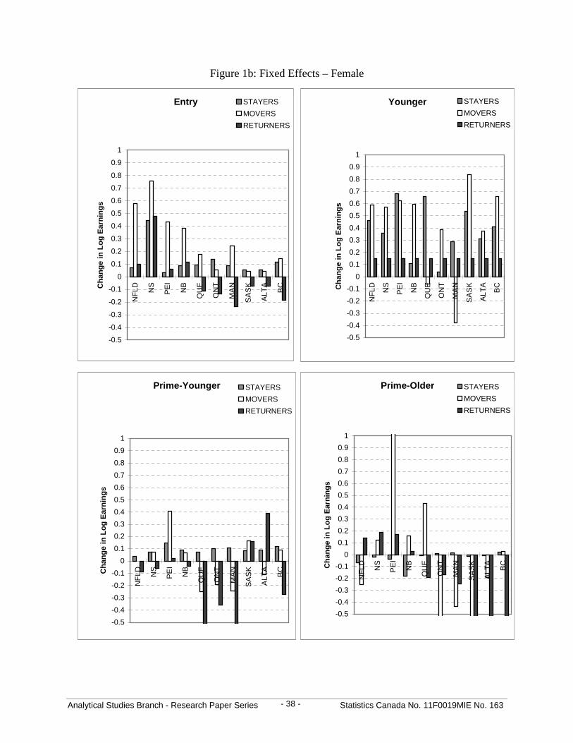
Analytical Studies Branch - Research Paper Series Statistics Canada No. 11F0019MIE No. 163- 38 -
Figure 1b: Fixed Effects – Female
Entry
-0.5
-0.4
-0.3
-0.2
-0.1
0
0.1
0.2
0.3
0.4
0.5
0.6
0.7
0.8
0.9
1
NF
LD NS
PE
I
NB
QU
E
ON
T
MA
N
SA
SK
ALT
A
BCC
han
ge
in L
og
Ear
nin
gs
STAYERS
MOVERS
RETURNERS
Prime-Older
-0.5
-0.4
-0.3
-0.2
-0.1
0
0.1
0.2
0.3
0.4
0.5
0.6
0.7
0.8
0.9
1
NF
LD NS
PE
I
NB
QU
E
ON
T
MA
N
SA
SK
ALT
A
BCCh
ang
e in
Lo
g E
arn
ing
s
STAYERS
MOVERS
RETURNERS
Prime-Younger
-0.5
-0.4
-0.3
-0.2
-0.1
0
0.1
0.2
0.3
0.4
0.5
0.6
0.7
0.8
0.9
1
NF
LD NS
PE
I
NB
QU
E
ON
T
MA
N
SA
SK
ALT
A
BCCh
ang
e in
Lo
g E
arn
ing
s
STAYERS
MOVERS
RETURNERS
Younger
-0.5
-0.4
-0.3
-0.2
-0.1
0
0.1
0.2
0.3
0.4
0.5
0.6
0.7
0.8
0.9
1
NF
LD NS
PE
I
NB
QU
E
ON
T
MA
N
SA
SK
ALT
A
BCCh
ang
e in
Lo
g E
arn
ing
s
STAYERS
MOVERS
RETURNERS

Analytical Studies Branch - Research Paper Series Statistics Canada No. 11F0019MIE No. 163- 39 -
References
Atkinson, A.B., F. Bourguignon and C. Morrison [1992]. Empirical Studies of Earnings Mobility(Switzerland: Harwood Academic Publishers).
Beach, Charles M. and Ross Finnie [1998]. “Earnings Mobility Benchmarks and LongitudinalPolarization in Canada, 1982-94”, Canadian Business Economics.
Courchene, Thomas J. [1970]. “Interprovincial Migration and Economic Adjustment”, CanadianJournal of Economics, V.3, N. 4 (November), pp. 550-76.
Courchene, Thomas J. [1974]. Migration, Income and Employment (Toronto: C.D. Howe Institute).
Day, Kathleen [1992]. “Interprovincial Migration and Local Public Goods”, Canadian Journal ofEconomics, V. XXV, N. 1 (February), pp. 123-44.
Day, Kathleen and Stan Winer [1994]. “Internal Migration and Public Policy: An Introduction to theIssues and a Review of Empirical Research in Canada”, in A. Maslove (ed.), Issues in the Taxationof Individuals (University of Toronto Press).
Dean, James M. [1992]. “Tax-Induced Migration in Canada 1972-79”, Western Economic Review,V. 1, N. 2, pp. 17-31.
Finnie, Ross [1997a]. “Earnings Patterns by Age and Sex in Canada, 1982-92”, Human ResourcesDevelopment Canada (Applied Research Branch) Research Paper R-97-11E). See also “EarningsPatterns by Age and Sex” (with Gaétan Garneau), Canadian Economic Observer, October, 1997,Statistics Canada Catalogue No. 11-010-XPB.
__________ [1997b]. “Stasis and Change: Trends in Earnings Levels and Inequality, 1982-92”,Canadian Business Economics, Vol. 5, No. 4 (Fall 1997), pp. 84-107.
__________ [1997c]. “Earnings Mobility in Canada, 1982-92”, Human Resources DevelopmentCanada (Applied Research Branch) Working Paper W-97-3Ea.
__________ [1997d]. “The Distribution of Earnings in a Dynamic Context in Canada, 1982-92”,Human Resources Development Canada (Applied Research Branch) Working Paper W-97-3Eb.
__________ [1997e]. “The Correlation of Individuals’ Earnings Over Time in Canada, 1982-92”,Human Resources Development Canada (Applied Research Branch) Working Paper W-97-3Ec.
__________ [1997f]. “A Dynamic Analysis of Low Market incomes (“Market Poverty”) ofCanadian Families With Children 1982-93”, Human Resources Development Canada (AppliedResearch Branch) Working Paper W-97-3Ed.
__________ [1997g]. “Unequal Inequality: The Distribution of Individuals’ Earnings by Province1982-94”, Human Resources Development Canada (Applied Research Branch) Working Paper.

Analytical Studies Branch - Research Paper Series Statistics Canada No. 11F0019MIE No. 163- 40 -
Finnie, Ross [1998a]. “Inter-Provincial Mobility in Canada: A Longitudinal Analysis”, HumanResources Development Canada (Applied Research Branch) Working Paper.
__________ [1998b]. “The Patterns of Inter-Provincial Migration in Canada 1982-95: Evidencefrom Longitudinal Tax-Based Data”, School of Policy Studies at Queen’s University mimeo.
__________ [1998c]. “Inter-Provincial Migration: A Longitudinal Analysis of Movers andStayers”, School of Policy Studies at Queen’s University mimeo.
__________ [2000]. “Who Moves? – A Panel Logit Model Analysis of Inter-Provincial MigrationIn Canada”, Research Paper No. 142. Analytical Studies Branch. Ottawa: Statisitics Canada.
Finnie, Ross and Charles Beach [1998]. “Earnings Mobility Benchmarks and LongitudinalPolarization in Canada, 1982-94” (with Charles M. Beach), Canadian Business Economics.
Finnie, Ross, and David Gray [1998]. “The Dynamics of the Earnings Distribution in Canada: AnEconometric Analysis”, Human Resources Development Canada (Applied Research Branch)Working Paper.
Grant, E. Kenneth and John Vanderkamp [1976]. The Economic Causes and Effects of Migration:Canada, 1965-7”, Economic Council of Canada (Ottawa: The Queen’s Printer).
___________ [1980]. “The Effects of Migration on Income: A Micro Study with Canadian Data1965-71”, The Canadian Journal of Economics, V. 13, N. 3 (August), pp. 381-406.
Greenwood, Michael [1975]. “Research on Internal Migration in the United States: A Survey”,Journal of Economic Literature, V. 13, pp. 397-433.
Lin, Zhengxi [1995]. “Interprovincial Labour Mobility in Canada: The Role of UnemploymentInsurance and Social Assistance”, Human Resources Development Canada (Evaluation Branch)Research Paper.
Marr, William L. and Frank W. Millerd [1980]. “Employment and Income Levels of Inter-Provincial Migrants Versus Non-Migrants, Canada 1971”, in Simon, J. L. and J. DaVanzo (eds.),Research in Population Economics, Vol. 2 (Greenwich, Conn.: JAI Press).
Mills, K. E., M. Percy and L. S. Wilson [1983]. “The Influence of Fiscal Incentives on InterregionalMigration: Canada 1961-78”, The Canadian Journal of Regional Science, V. VI, N. 2 (Autumn),pp. 207-229.
Nakosteen, Robert A. and Michael Zimmer [1980]. “Migration and Income: the Question of Self-Selection”, Southern Economic Journal, V. 46, pp. 840-51.
OECD [1996]. Employment Outlook, Chapter 3: “Earnings Inequality, Low-Paid Employment andEarnings Mobility”, pp. 59-108 (Paris: Organization for Economic Co-operation and Development).
Osberg, Lars, Daniel Gordon and Zhengxi Lin [1994]. “Interregional Migration and InterindustryLabour Mobility in Canada: A Simultaneous Approach”, Canadian Journal of Economics, V.XXVII, N. 1 (February), pp. 58-80.

Analytical Studies Branch - Research Paper Series Statistics Canada No. 11F0019MIE No. 163- 41 -
Robinson, Chris and Nigel Tomes [1982]. “Self-Selection and Interprovincial Migration inCanada”, Canadian Journal of Economics, V. XV, N. 3 (August), pp. 474-502.
Rosenbluth, Gideon [1996]. “Interprovincial Migration and the Efficacy of Provincial Job CreationPolicies”, Canadian Business Economics, Vol. 4, No. 2 (Winter), pp. 22-35.
Shaw, R. Paul [1986]. “Fiscal Versus Traditional Market Variables in Canadian Migration”,Journal of Political Economy, V. 94, N. 3, pp. 648-666.
Sjaastad, Larry [1962]. “The Costs and Returns of Human Migration”, Journal of PoliticalEconomy (Supplement), V. 70, pp. 80-93.
Vanderkamp, John [1988]. “Regional Disparities: A Model with Some Econometric Results forCanada”, pp. 269-96 in Higgins, B. and D. J. Savoie (eds.), Regional Economic Development:Essays in Honour of François Penoux (Boston: Unwin Hyman).
Vachon, Marc and François Vaillancourt [1998]. “Interprovincial Mobility in Canada, 1961-1996:Trends and Determinants”, in Lazar, Harvey (ed.), Centre for Intergovernmental Relations, Queen’sUniversity at Kingston, Ontario.
Winer, Stanley L. and Denis Gauthier [1982]. Internal Migration and Fiscal Structure, EconomicCouncil of Canada (Ottawa: Supply and Services Canada).