THE EFFECTS OF FISCAL DECENTRALIZATION ON LOCAL …

THE EFFECTS OF FISCAL DECENTRALIZATION ON LOCAL PUBLIC FINANCE

IN KOREA: PUBLIC SPENDING, FUNCTIONAL RESPONSIBILITY,

AND FISCAL INDEPENDENCE

by

OSUNG KWON

(Under the direction of Thomas P. Lauth)

ABSTRACT

In recent years, fiscal decentralization has been advocated worldwide. The common motive is that fiscal decentralization is considered to have the potential to improve the performance of the public sector. However, some recent studies hold that the conventional argument that fiscal decentralization will increase economic efficiency in the public sector may not be applicable in developing countries. Also, the conventional argument regarding functional assignment has been challenged on several grounds. The recent development of local autonomy and fiscal decentralization in Korea provides an excellent opportunity for empirical investigation of this subject. Because Korea represents the borderline between developed and developing countries, a decentralization study of such a country will contribute to testing the contention that there is no efficiency gain in developing countries, as well as investigating the issue of functional assignment outside developed countries. To date, there have been few efforts to systematically analyze the actual effects of decentralization on the overall public sector in Korea. This study asks three questions. First, has fiscal decentralization affected the size of the public budget in Korea? Second, what changes occur in functional responsibility after the onset of fiscal decentralization? Third, what are the effects of decentralization on the fiscal independence of local governments? The study employs regression analysis to test three hypotheses. We find decentralization improves economic efficiency and accountability in the Korean public sector. The levels of developmental and redistribution expenditures increase as decentralization proceeds in Korea. Finally, the degree of decentralization is positively associated with the degree of the fiscal independence of local governments. INDEX WORDS: Fiscal decentralization, Fiscal federalism, Korean local finance, Decentralization hypothesis, Functional responsibility, Fiscal independence, Generalized Least Square (GLS), Two Stage Least Square (2SLS), Random effects model




by

OSUNG KWON

B.A., Sungkyunkwan University, Korea, 1986

M.P.A., West Virginia University, 1993

A Dissertation Submitted to the Graduate Faculty of The University of Georgia in Partial

Fulfillment of the Requirements for the Degree

DOCTOR OF PUBLIC ADMINISTRATION

ATHENS, GEORGIA

2002

2002

Osung Kwon

All Rights Reserved




by

OSUNG KWON

Approved:

Major Professor: Thomas P. Lauth Committee: Richard W. Champbell Jerome S. Legge, Jr. Laurence J. O�Toole, Jr. Hal G. Rainey Electronic Version Approved: Gordhan L. Patel Dean of the Graduate School The University of Georgia August 2002

iv

ACKNOWLEDGMENTS

I would like to express my appreciation to Dr. Thomas P. Lauth, who rendered me

priceless encouragement and the best direction. Also, I appreciate the other members of

the dissertation committee � Dr. Richard W. Champbell, Dr. Jerome S. Legge, Jr., Dr.

Laurence J. O�Toole, Jr., and Dr. Hal G. Rainey � whose comments and suggestions have

substantially improved the quality of this dissertation.

My family deserves my deepest feelings of gratitude and love. My father, mother, and

four sisters sacrificed a great deal for my education. Especially, I owe thanks to my wife,

Okjeung, and my lovely daughter and son, Lee-jin and Hyuk-chan. Without their patience

and love, completion of my study would have been impossible.

v

TABLE OF CONTENTS

Page

ACKNOWLEDGMENTS............................................................................................... iv

LIST OF TABLES ........................................................................................................vii

LIST OF FIGURES........................................................................................................ ix

CHAPTER

1 INTRODUCTION...............................................................................................1

1.1. Introduction............................................................................................1

1.2. Importance of This Study........................................................................5

1.3. A Rationale for Governmental Action......................................................6

1.4. Multiunit Provision of Public Goods......................................................11

1.5. Fiscal Federalism...................................................................................16

1.6. Summary...............................................................................................19

2 FISCAL FEDERALISM IN KOREA.................................................................21

2.1. Local Autonomy and Fiscal Decentralization in Korea...........................21

2.2. Fiscal Structure of Local Government in Korea .....................................27

2.3. Summary...............................................................................................63

3 HYPOTHESES AND LITERATURE REVIEW ...............................................65

3.1. The Effect of Decentralization on the Size of Public Budget ..................65

3.2. The Change in Local Government Expenditure Structure ......................79

vi

3.3. Decentralization�s Effect on Fiscal Independence of

Local Governments...............................................................................90

3.4. Summary...............................................................................................94

4 DATA ANALYSIS AND RESULTS.................................................................95

4.1. The Econometric Approach...................................................................95

4.2. Data and Sources ..................................................................................96

4.3. Empirical Test of Hypothesis 1..............................................................98

4.4. Empirical Test of Hypothesis 2............................................................112

4.5. Empirical Test of Hypothesis 3............................................................125

5 SUMMARY AND CONCLUSION .................................................................133

APPENDICES

A A Glossary of Tax Terms ................................................................................140

B An Example of Calculation of Standardized Cost in A city...............................141

C Fiscal Decentralization Survey Questionnaire...................................................143

D Regression Estimations without Controlling Grant Effects...............................146

REFERENCES............................................................................................................149

vii

LIST OF TABLES

Page

Table 1.1. Examples of Externalities................................................................................8 Table 2.1. Local Government Share of Total Taxes.......................................................26 Table 2.2. Local Government Share of Total Government Expenditures........................26 Table 2.3. Self-reliance Rate of Local Government........................................................27 Table 2.4. Composition of Local Finance, 1998.............................................................28 Table 2.5. Composition of Revenue Sources of Education Special Account, 1998.........30 Table 2.6. Local Autonomy Units in Korea (1998 and 1991) .........................................31 Table 2.7. Expenditure Shares of General, Enterprise Special, and Other Special Account, 1998 .......................................................................32 Table 2.8. Composition of Local Revenues by Source ...................................................33 Table 2.9. Composition of Local Revenue by Autonomy Unit, 1998..............................34 Table 2.10. Composition of Local Tax ...........................................................................41 Table 2.11. Local Tax by the Type of Government (1998)..............................................43 Table 2.12. The Ratio of Earnings to Operating Costs in User-charge Items...................44 Table 2.13. Composition of Local Revenues by Account, 1998 ......................................45 Table 2.14. Composition of Non-Tax Revenue...............................................................46 Table 2.15. Share of Intergovernmental Revenues to Total Local Revenues ...................48 Table 2.16. Composition of Intergovernmental Grants by Autonomy Units, 1998...........49 Table 2.17. Functional Classification of Local Expenditure by Account, 1995 ................59 Table 2.18. Functional Classification of Local Expenditure by Government Unit, 1995...60

viii

Table 2.19. Changes of Local Expenditure Share by Functions 1986-1995 .....................62 Table 3.1. The Ratio of Total Tax Revenue-to-GNP in Selected Countries, 1987 ..........71 Table 3.2. The Ratio of the Central Tax Revenue-to-GNP in Selected Countries, 1987..........................................................................71 Table 4.1. Frequency of Survey Response by the Type of Government ..........................98 Table 4.2. Operationalization of Variables (Hypothesis 1) .............................................99 Table 4.3. OLS Estimation of CE, LE, and TE............................................................100 Table 4.4. OLS Estimation of CE, LE, and TE with Control Variables ........................101 Table 4.5. GLS Estimation of CE, LE, and TE............................................................104 Table 4.6. 2SLS Estimation of CE...............................................................................109 Table 4.7. OLS, GLS, and 2SLS Estimation of CE, LE, and TE without Defense Expenditure .....................................................................111 Table 4.8. Operationalization of Variables (Hypothesis 2) ...........................................113 Table 4.9. OLS Estimation of RED and DEV..............................................................116 Table 4.10. GLSE Estimation of RED and DEV ..........................................................124 Table 4.11. Operationalization of Variables (Hypothesis 3) ..........................................127 Table 4.12. OLS Estimation of SER.............................................................................128 Table 4.13. GLSE Estimation of SER (1987 � 1998) ...................................................129 Table 4.14. GLS Estimation of SER (1987 � 1994)......................................................130 Table 4.15. GLS Estimation of SER (1992 � 1998)......................................................131

ix

LIST OF FIGURES

Page

Figure 1.1. Underproduction with a Positive Externality..................................................8 Figure 1.2. Overproduction with a Negative Externality ..................................................9 Figure 1.3. Correspondence between the Benefit Area and the Size of Government.......12 Figure 1.4. Welfare Loss due to Centralized Provision ..................................................14 Figure 3.1. The Optimal Provision of Government and Private Goods ...........................70 Figure 4.1. Defense Expenditure to GDP (1981 � 1998)..............................................111 Figure 4.2. Structure of the Heteroscedasticity (RED).................................................118 Figure 4.3. Structure of the Heteroscedasticity (DEV) ................................................119

1

CHAPTER 1

INTRODUCTION

1.1. Introduction

In recent years, fiscal decentralization has been advocated worldwide. Examples are

abundant around the world: functional devolution by the Reagan administration in the

U.S., decentralization of fiscal decision-making and public administration in Latin

American countries, and economic reforms (from centralized to decentralized economies)

in Asian countries.

While fiscal decentralization has several reasons for being adopted around the world,1

the common motive is that fiscal decentralization is considered to have the potential to

improve the performance of the public sector (Oates, 1999:1120). Of three major

economic functions of governmental action � allocation, redistribution, and stabilization

(Musgrave, 1959), the key question of fiscal federalism is which level of government

should undertake what function, and on whose budget? The theory holds that for certain

public goods or services such as local public goods, providing them in a decentralized

fashion can increase efficiency2 and accountability in resource allocation because (1) local

governments can be better tailored to the geographical areas in which public goods are

distributed, (2) local governments are better positioned to recognize local preferences and

needs, and (3) pressure from inter-jurisdictional competition may motivate local

1 Bird and Vaillancourt (1998) identify four reasons especially in developing countries: (1) economic efficiency, (2) cost efficiency, (3) accountability, and (4) resource mobilization. 2 Throughout this dissertation the term �efficiency� means economic efficiency (Pareto optimal) unless indicated otherwise.

2

governments to be innovative and accountable to their residents (Oates, 1972). The

theory also holds that the redistribution and stabilization functions, as well as provision of

national public goods such as national defense in the allocation function should be the

central government�s task (Musgrave, 1959; Oates, 1972).

However, this conventional argument has been challenged on several grounds. For the

redistribution and stabilization functions, several recent empirical studies challenge the

conventional wisdom. For the allocation function of local public goods, recent studies

argue that the conventional wisdom may remain true in developed countries, but it is not

the case in developing countries. They hold that the conventional argument that

decentralized provision of public goods will increase efficiency in resource allocation may

not be applicable in developing countries (Bahl and Linn, 1994; Prud�homme, 1995). The

reason is that most developing countries do not meet implicit or explicit assumptions

posed by fiscal federalism theory. In developing countries, for example, local voter

preferences may not be as readily reflected in local budget outcomes as in developed

countries. Local governments have weak administrative capacity to carry out their own

fiscal decisions. Without independent decision-making capacity in determining the

quantity and quality of public goods provided and sources of finance that internalize the

costs, decentralized provision of local public goods may not increase efficiency. Rather,

centralization is more suited in this situation because it may take advantage of scale

economies in production of public goods and services. Also, fiscal centralization may be a

more effective tool for economic stabilization, economic growth, income redistribution,

and tax administration. These are very critical pending issues in developing economies.

3

A review of international determinant studies regarding decentralization has found that

stage of economic development in a country, measured by income, urbanization, and

Gross Domestic Product (GDP), is associated with a significantly greater subnational

share of expenditure (Kee, 1977; Bahl and Nath, 1986; Wasylenko, 1987; Pinizza, 1999).

Bahl and Linn (1992:393) conclude, �[t]he implication of this observation is that

government policies to promote fiscal decentralization are more likely to be effective for

[developed] countries.�

As a result, most empirical studies on the subject of fiscal decentralization are limited

to developed countries. However, fiscal decentralization takes place not only in

developed countries, but also in developing countries. Although there are several studies

covering a specific developing country, they are all descriptive. Typically, they describe

the current fiscal structure, assess a new decentralization program, and identify possible

problems and their solutions (e.g., Fukasaku and Mello, 1999; Bennnett, 1994; Bird and

Vaillancourt, 1998; Ahmad, 1997).

Missing from the literature is a systematic analysis of the actual effects of

decentralization on the overall public sector in developing countries. The recent

development of local autonomy and fiscal decentralization in Korea provides an excellent

opportunity in this matter. Also, because Korea represents the borderline between

developed and developing countries, a decentralization study of such a country will

contribute to testing the validity of the contention that there is no efficiency gain in

developing countries. Until now, there have been few efforts to systematically analyze the

actual effects of decentralization on the overall public sector in Korea.

4

This study asks three questions about the actual effects of decentralization on the fiscal

structure in Korea. First, has fiscal decentralization affected the size of the public budget

in Korea? A decentralized system is expected to respond better to local preferences and

needs and to promote competition among local units in the provision of public goods and

services. The better fitted provision of public goods and services and competition will

result in a more efficient and less wasteful provision of public goods and services, thus

affecting the size of the budget.

Second, what changes occur in functional responsibility as the degree of fiscal

decentralization increases? The conventional argument for assignment of functions is that

the central government should be engaged in stabilization and redistribution functions

while sub-national governments should be engaged in the allocation of local or regional

public goods (Musgrave, 1959; Oates, 1972). However, the conventional wisdom has

been challenged on several grounds. The role of local governments in the stabilization

function and the redistribution function has been re-evaluated. Some empirical studies

provide a rationale for subnational stabilization and redistribution policies (Gramlich,

1987; Pauly, 1973). Still, the issue is unresolved. Therefore, it is interesting to investigate

the issue outside the United States.

Third, what are the effects of decentralization on fiscal independence of local

governments? One major argument for deferring local autonomy implementation in Korea

is that local governments were heavily dependent upon intergovernmental transfers to

finance local public goods and services. A degree of fiscal independence in local

government is critical for efficiency gain in the provision of local public goods. Also,

without adequate revenue-raising capacity, the capacity of independent fiscal decision-

5

making in local governments is limited. Therefore, it is important to investigate changes in

the fiscal independence of local governments as decentralization proceeds.

1.2. Importance of This Study

This study is important in several respects. First, many decentralization studies have

tended to be polemical rather than analytical or empirical (Wolman, 1994:249). Many

benefits of fiscal decentralization policies are based on theoretical arguments. Therefore,

it is important to test these theoretical arguments in an empirical setting.

Second, most empirical decentralization studies are limited to the U.S. The few

existing exceptions represent similar government structure to that of the U.S. However,

Oates (1977:4) holds that �in economic terms, all governmental systems are more or less

federal. Even in a formally unitary system, there is typically a considerable extent of de

facto fiscal discretion at decentralized levels.� Therefore, to generalize fiscal federalism

theory, it is an important step to extend the study area � from federal to unitary structure.

Third, most empirical studies on the subject of fiscal decentralization are limited to the

developed countries. Many scholars argue this situation exists because most developing

countries do not meet implicit or explicit assumptions posed by fiscal federalism theory.

Another reason may be the difficulty of obtaining reliable fiscal data from developing

countries. In order to assess the worldwide phenomenon accurately, we need a systematic

analysis of fiscal decentralization in developing countries.

Fourth, this study may help to formulate future intergovernmental fiscal policy in

Korea. Because the current development of fiscal decentralization is a relatively new

phenomenon in Korea, policy-makers desperately need much more input on this matter.

6

As a subfield of public finance, fiscal federalism is concerned with the vertical structure

of the public sector. The traditional concerns of the fiscal federalism literature are what

functions and instruments should be decentralized or centralized and what welfare gains

are recognized from decentralization. Recently, these traditional concerns have been

expanded to several new topics: laboratory federalism, interjurisdictional competition, the

political economy of fiscal federalism, market-preserving federalism, and fiscal

decentralization in the developing economy (Oates, 1999). This study contributes to some

of these new topics of the fiscal federalism literature.

1.3. A Rationale for Governmental Action

Human desires for goods and services are seemingly unlimited. But our resources to

satisfy them are limited. Economists refer to the imbalance between them as scarcity. The

discipline of economics studies how scarce resources are allocated among alternative uses

(Hyman, 1993:3). A free competitive market and pricing system has been recognized as

an efficient system to allocate scarce resources as long as it meets four conditions �

perfect competition, information, complete market, and exclusion and rival consumption.3

When any or all of the four conditions mentioned above are not satisfied, economists

refer to this outcome as market failure. Market failure makes the free private competitive

3 (1) Perfect Competition: A perfectly competitive market means producers have no power in setting the price. They accept the price as given and sell as much as they can at that price. (2) Information: Asymmetric information is the condition that prevails in a market in which some

participants are better informed about the quality of a product than are the participants with whom they trade. The problem is that the less complete the information, the more likely the buyer will make the incorrect selection. That unintentional error in judgement can lead to an inefficient pattern of resource use.

(3) Complete Market: If the cost of production is more than the amount that people are willing to pay for goods, there will be no market for that goods.

(4) Nonexclusivety and nonrivalry are the nature of public goods.

7

market no longer efficient in resource allocation, thus providing a rationale for

governmental action.

Among those conditions in which market failure takes place, scholars of public finance

have paid special attention to the nature of public goods because it is related directly to

the issue of public provision of goods and services. Pure public goods have two basic

distinguishing characteristics: nonexclusivety and nonrivalry in consumption.

Nonexclusivety in consumption means that consumption cannot be withheld from

consumers who choose not to pay the price. When the good is nonexclusive, the

transaction costs of excluding a person from obtaining it are extremely high. Nonrivalry in

consumption means consumption of a given quantity of a good by any one person does

not reduce the availability of the good to others. Therefore, the marginal cost of allowing

an additional consumer to enjoy the benefits of the goods is zero until the presence of

congestion. In practice, beyond some level of consumption the marginal social cost of

consumption can become positive because the good is congested.

Besides market failure stemming from the nature of public goods, there are three

reasons that justify governmental action in the marketplace (Musgrave and Musgrave,

1989:42). First, a market solution is not efficient in resource allocation if there are

�externalities,� which are costs or benefits of market transactions not reflected in prices.

In other words, �An externality is any valued impact (cost or benefit) resulting from any

action (whether related to production or consumption) that affects someone who did not

fully consent to it� (Weimer and Vining, 1992:57). Examples are shown in Table 1.1.

8

Table 1.1. Examples of Externalities Positive Negative Producer-to-producer

Warm water from nuclear power plant used by downstream fish farmers

Toxic chemical pollution harming downstream commercial fishing

Producer-to-consumer

Private timber forests providing scenic benefits to nature lovers

Air pollution from factories harming lungs of people living nearby

Consumer-to-consumer

Immunization by persons against contagious disease helping protect others

Cigarette smoke from one person reducing enjoyment of meal by another

Consumer-to-producer

Unsolicited letters from consumers providing information on product quality

Disturbing of domestic farm animals by game hunters

Source: Weimer and Vining (1992:59)

Price

S

MSB

MPB Q1 Q* Quantity

Figure 1.1. Underproduction with a Positive Externality

Figure 1.1 illustrates the resource allocation effects of a positive externality in

production. In the presence of a positive externality, producers will produce too little of

9

the good that generates the externality. For example, the individual student is willing to

pay the price for education depending on his or her own utility, not depending on the

overall effect of his or her education on society. Therefore, quantity for education is

chosen at Q1 at which supply schedule (S) intersects marginal private benefit schedule

(MPB). But economic efficiency requires that marginal social benefits (MSB) and

marginal social costs (which is supply schedule) be equal at the selected output level.

Therefore, efficient output level should be at Q*.

Price MSC

MPC

D

Q* Q1 Quantity

Figure 1.2. Overproduction with a Negative Externality

Figure 1.2 illustrates a negative externality. In the presence of a negative externality,

producers will produce too much of the goods that generate the externality. For example,

if the goods are a chemical product, marginal private cost (MPC) represents the marginal

amounts the firm has to pay for the raw materials, labor, and other things needed for the

final product. Therefore, quantity for the chemical product is chosen at Q1 at which MPC

10

intersects demand schedule (D). But the marginal private cost does not reflect the

negative impacts of the pollution that is a byproduct of the manufacturing process. If we

can find out how much each person is willing to pay to avoid the pollution at each output

level, then we can add these amounts to the marginal costs. That will be the marginal

social cost (MSC). Economic efficiency requires that marginal social benefits (which is

demand schedule) and marginal social costs be equal at the selected output level.

Therefore, efficient output level should be at Q*.

According to Musgrave and Musgrave (1989), another reason that justifies

governmental action in the marketplace is that society does not like the results of resource

allocation even though the market is working efficiently. According to an agreed-upon

normative standard, society judges what is a fair and equitable distribution of income and

goods and services. In this case, society charges government with altering the market

outcomes to confirm with the normative standard. A third reason for governmental action

is related to macroeconomic problems. A competitive free market cannot guarantee full

employment, price stability, and economic growth.

Musgrave (1959) terms these three functional areas of governmental action: allocation,

redistribution, and stabilization. The allocation function covers all public policies that

restore an efficient allocation of resources that the market cannot perform because of the

nature of public goods and externalities. The redistribution function includes public

policies that make the actual distribution of income and wealth fair and equitable

according to society�s normative standard. The stabilization function refers to public

policies that are designed to insure full employment, price stability, and economic growth.

11

1.4. Multiunit Provision of Public Goods

If we look at the real world, we can hardly find any nation that has only one

governmental unit. For example, South Korea, which is a relatively small country, has

about 250 governmental units.4 The US has about 80,000 governmental units. In reality,

therefore, multi-governmental units, not one governmental unit, perform the three

governmental functions mentioned above in both nations. This multiunit governmental

structure leads us to ask why we need multi-governmental structures instead of one big

government. Obviously, this multiunit governmental structure reflects each nation�s social

and political history. Models of federalism attempt to define the relationships between the

national government and subnational governments (Leach, 1970; Lauth and Douglas,

1995). A competitive theory of federalism characterizes the relationships as competing for

power. It includes nation-centered federalism, state-centered federalism, and dual

federalism. An interdependent theory of federalism emphasizes the interaction among

levels of government, especially interactions based upon allocation of financial grants and

aids. It includes cooperative federalism, creative federalism, and new federalism (which

sought to reallocate functional responsibilities among national, state, and local levels of

government). Although theories of federalism may explain much about the role of the

national government and its fiscal relationship with subnational governments, they do not

provide a complete explanation of intergovernmental relations.

In addition to history and political theory, there are also economic reasons for the

multiunit governmental structure. According to Musgrave (Musgrave, 1959; Musgrave

and Musgrave, 1989), the economic rationale for multiunit governmental provision of

4 The governmental unit means a government that has taxing and expenditure power.

12

public goods is that each public good in question has a different geographical benefit area.

The benefit area is a geographical area over which public good�s quality remains

unchanged (Raimondo, 1992:51). In the case of fire protection, for example, its benefit

area is small or local because the distance between a fire station and an individual

household affects the quality of fire protection. For the case of national defense, its

benefit area is large or nationwide because individuals receive the same quality of defense

service regardless of where they live. Efficient allocation of resources requires that �each

jurisdiction provide services the benefits of which accrue within its boundaries, and it use

only such sources of finance as will internalize the costs� (Musgrave and Musgrave,

1989:447). Therefore, the provision of a specific good should be assigned according to its

benefit area.

Benefit area Government Overlap of Benefit area with Government Government Benefit area

Case I Case II Case III

Figure 1.3. Correspondence between the Benefit Area and the Size of Government (Raimondo, 1992:55)

Figure 1.3 illustrates the degree of correspondence to which the benefit area and the

size of a governmental unit match.5 In the case I, the benefit area is greater than the size

5 The governmental unit is assumed to fully internalize the costs within its jurisdiction.

13

of the government. This situation is called a benefit spillover (or spatial externality). Like

the positive externality, the residents underestimate the true social benefit and demand too

little of the good or service. In the case II, the benefit area is smaller than the size of the

government. All residents pay for the good or service, but only some of the people

receive it. This situation is called a cost spillover. Like the negative externality, the

people who receive the benefit underestimate the true social cost and demand too much.

The case III has a perfect match between the benefit area and the size of the governmental

unit. In this case, because the quantity will be chosen at the point where the marginal

social benefit equals perfectly the marginal social cost of the provision, the resulting

resource allocation is efficient.

Musgrave and Musgrave (1989:447) conclude that

The spatially limited nature of benefit incidence calls for a fiscal structure composed of multiple services units, each covering a different-sized region within which the supply of a particular service is determined and financed�. Some services call for nationwide, others for statewide, and still others for metropolitan-area-wide or local units.

Until now, we have discussed the rationale for multiunit provision of public goods only

in terms of the spatial dimension of goods in question. Besides that, there are other

considerations that we should take into account for the multiunit provision of public

goods. If all people desire the same amount and type of a specific service, for example

police protection, then there is no reason for more than one governmental unit, which will

be a large one, to provide uniform police protection service across the nation (assuming

that the benefit area of police protection is nationwide). But if people differ in their

preferences for police protection service, many people will be dissatisfied with the uniform

14

level of service. The efficient solution is to provide a different level of police service

depending on people�s preferences. Moreover, as Tiebout (1956) argues, if consumers

can choose residential location freely depending on their preferences for service/tax

packages, the advantage of a multiunit governmental structure is strengthened because the

residential sorting may increase heterogeneous demands and differential tax prices across

jurisdictions.

A welfare loss due to centralized provision of public goods is illustrated in Figure 1.4.

Two groups have different demands for a particular public good. Demand curve 1 (D1)

represents the demand of group 1 while demand curve 2 (D2) represents the demand of

group 2. Let us assume the unit price of the public good is fixed at P. A government

provides a single level of quantity at Qc. For group 1, the government overprovides the

public good. For group 2, the government underprovides the public good. Welfare loss

due to unitary provision is represented by two shaded areas, which are ABC and CEF.

Therefore, if the provision of the public good is decentralized at Q1 and Q2, the welfare

loss, the sum of ABC and CEF in this particular example, will disappear.

Price F P A C E B D2 D1 Q1 Qc Q2 Output

Figure 1.4. Welfare Loss due to Centralized Provision (Oates, 1977:10)

15

This consumers� surplus analysis implies another point. The magnitude of the welfare

loss from centralized provision is dependent upon the variation in individual demands. For

example, if the distance between Q1 and Q2 were much longer than the distance presented

in Figure 1.4, the welfare loss, that is, the sum of ABC and CEF could be larger.

Therefore, the magnitude of efficiency gain from decentralized provision is critically

dependent upon the extent of heterogeneous demands and differential tax prices across

jurisdictions (Oates, 1977:10).

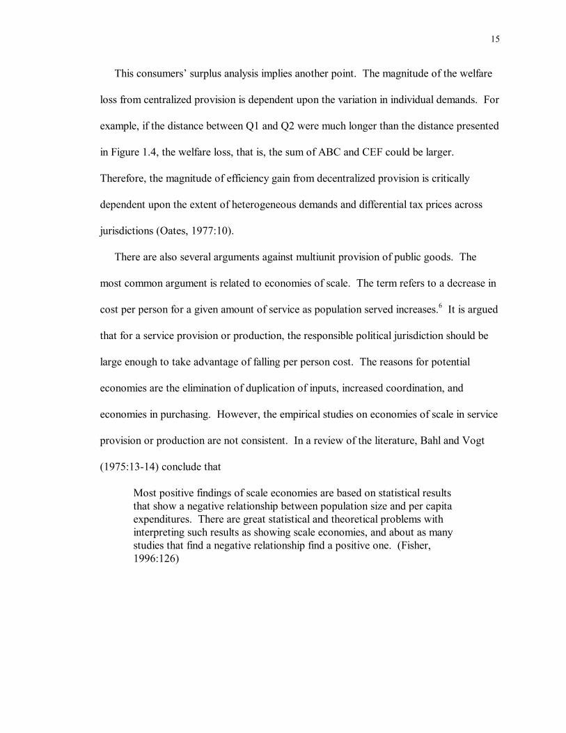
There are also several arguments against multiunit provision of public goods. The

most common argument is related to economies of scale. The term refers to a decrease in

cost per person for a given amount of service as population served increases.6 It is argued

that for a service provision or production, the responsible political jurisdiction should be

large enough to take advantage of falling per person cost. The reasons for potential

economies are the elimination of duplication of inputs, increased coordination, and

economies in purchasing. However, the empirical studies on economies of scale in service

provision or production are not consistent. In a review of the literature, Bahl and Vogt

(1975:13-14) conclude that

Most positive findings of scale economies are based on statistical results that show a negative relationship between population size and per capita expenditures. There are great statistical and theoretical problems with interpreting such results as showing scale economies, and about as many studies that find a negative relationship find a positive one. (Fisher, 1996:126)

16

1.5. Fiscal Federalism

Fiscal federalism generally describes the division of governmental functions and

revenue powers between entities in a multilevel government system. The key question of

fiscal federalism is which government should undertake what activity, and on whose

budget?

The term �federalism� may have multiple meanings depending on how or where it is

used.7 In this study, the focus is on economic usage. In economic terms, fiscal federalism

is defined as the study of multilevel finance (Oates, 1977). In this sense theories of fiscal

federalism may be applied for a country in a formally unitary system because there is

typically a considerable extent of de facto fiscal discretion at decentralized levels even in

that country.

According to Musgrave (1959), stable economic growth and the redistribution of

income are appropriate objectives of the central government while the allocation function

should be assigned to other levels of government depending on the nature of goods and

services. However, theorists differ regarding the proper assignment of functions in the

first two areas: stabilization and redistribution.

For the stabilization function, the conventional argument is that subnational economies

are so open that the effects of local stimulative policy disperse throughout the whole

economy. This argument is based on the idea of spatial externality. That is, if a benefit is

not held within the area where the benefit is financed, the resulting resource allocation is

6 In standard microeconomic usage, economies of scale refers to a decrease in average cost as the quantity of output rises. 7 For a legal study, federalism generally refers to a constitutional framework. In the field of political science, the term is used to cover a wide range of studies such as research on federal institutions, intergovernmental policy formulation, and implementation.

17

not efficient. A remedy is that the cost area is increased according to the benefit area.

Therefore, the central government should undertake stabilization policy.

However, this conventional argument has been challenged on several grounds. Some

studies provide a rationale for subnational economic development policy. Gramlich

(1987) holds that many subnational economic development policies have greater effects

within the jurisdiction. And, increasingly, macroeconomic problems are regional rather

than national. Therefore, to solve the regional macroeconomic problems may require

regional rather than national policy.

For the redistribution function, the conventional argument follows the same logic as in

the stabilization function. The benefit of a redistribution policy in a subnational

government cannot be held within the jurisdiction because of free mobility of population.

For example, if a state has a generous welfare benefit package for lower income families,

the residents in nearby states, which have less generous welfare programs, might migrate

into the state that has a generous program. Meanwhile, higher-income taxpayers might

move to a different state where less generous welfare program exists. Because of this

externality, the conventional argument holds that the central government should undertake

the redistribution function.

However, some studies show that few welfare recipients actually move to other states

to receive higher welfare benefits (Homer, 1975). Moving is costly and other locational

factors may offset redistributional incentives. If mobility of welfare recipients among

jurisdictions is trivial, there may be an efficiency rationale for redistribution at the

subnational level because subnational governments are better able to express regionally

diverse preferences for redistribution (Pauly, 1973).

18

On the revenue side, each level of government requires fiscal instruments to carry out

the assigned functions. Then, the issue will be �Which taxes are best suited for use at the

different levels of government?� (Oates, 1999:1125)

As mentioned earlier, efficient allocation of resources requires that each jurisdiction

should provide services the benefits of which accrue within its boundaries, and that it

should use only such sources of finance as will internalize the costs. Therefore, efficiency

requires that the beneficiaries of each benefit jurisdiction pay for the services, which that

jurisdiction provides. Accordingly, if the benefit region is nationwide, then a national tax

is necessary. If the benefit region is local, then a local tax is more logical.

Because of the inherent nature of taxation, however, the link between spending and

taxing is not always explicit. In other words, taxation cannot always follow this benefit

principle. Therefore, there is a need for compromise in which efficiency cost is minimal in

a given situation. Considering this fact, Musgrave (1983) suggests the following

principles for tax assignment.

1. Highly progressive taxes, especially for redistributional purposes, should be centralized. Such taxes are to be avoided at decentralized levels of government because of the perverse incentives they create for migration among jurisdictions.

2. In general, lower-level governments should eschew taxes (at least nonbenefit taxes) on highly mobile tax bases. Such taxes can distort the locational pattern of economic activity. Decentralized governments are better advised to employ taxes on relatively immobile tax bases (such as land).

3. The central government should exercise primary taxing authority over those tax bases that are distributed across jurisdictions in a highly unequal fashion. Taxes on deposits of natural resources, in particular, should be centralized to avoid geographical inequities and to prevent allocative distortions that can result from the local taxation of such resources.

4. While user taxes and fees have much to commend them at all levels of government as benefit taxes, they are an especially appealing revenue

19

instrument at the most decentralized levels of government. They create, in principle, no potentially distorting incentives for movements among jurisdictions. (recited from Oates (1994:131))

This prescription may be summarized that nonbenefit taxes should be assigned to the

central level and benefit taxes should be assigned to the local level in order to minimize

economic distortion induced by taxes, based on the following assumptions: (1) the

mobility cost of economic units such as labor, capital, etc. increases as the geographical

size of jurisdiction increases and (2) people are more willing to pay taxes if they receive

services they value.

However, there are few empirical studies on this issue. Some recent studies explore

the efficiency costs induced by local income tax (Goodspeed, 1989) and local taxation of

natural resources (Mieszkowski and Toder, 1983). They conclude that the economic

distortions by such taxes are marginal so that the constraint on the local use of ability-to-

pay taxation is somewhat exaggerated and the restraint on the local taxation of natural

resources may be justified only according to the equity standard. The issue is not settled.

As Oates (1994:133) holds, therefore, �we have some general prescriptions for the

assignment of revenue instruments to different levels of government. But we badly need a

better empirical sense of just what is at stake here.� The research undertaken in this

dissertation will contribute to improving our understanding of this issue.

1.6. Summary

This chapter stated three research questions and presented arguments regarding the

importance of this study. According to Musgrave (1959), three major economic functions

20

of governmental action are allocation, redistribution, and stabilization. The nature of

public goods and externalities provide a rationale for the allocation function. Income

redistribution and macroeconomic issues provide a rationale for the redistribution and

stabilization functions.

A key argument for decentralization is that the decentralized provision of public goods

increases efficiency in resource allocation because the quantity of the public goods can be

better adjusted to citizens� preferences. The key question of fiscal federalism is which

level of government should undertake what function, and on whose budget?

In the case of functional assignment among the levels of government, the conventional

argument prescribes that subnational governments should be engaged in the allocation

function, while the central government should be engaged in the redistribution and

stabilization functions. Musgrave (1959) and Oates (1972, 1977) provide a theoretical

rationale for this prescription. However, some empirical studies provide a rationale for

subnational redistribution and stabilization policies (Homer, 1975; Pauly, 1973; Gramlich,

1987). Because of this conflicting view, it is useful to re-examine this issue.

In the case of the assignment of revenue instruments, the conventional argument is that

the beneficiaries of each jurisdiction should pay for the services which the jurisdiction

provides. However, some empirical studies find that local use of ability-to-pay taxation

may induce only marginal economic distortion. Therefore, we need a better empirical

understanding of this issue.

In the next chapter, we review the recent development of local autonomy and fiscal

decentralization in Korea. We also describe fiscal structure of local governments in Korea

for a better empirical sense of the issues.

21

CHAPTER 2

FISCAL FEDERALISM IN KOREA

In the previous chapter, we reviewed theoretical arguments concerning fiscal

decentralization. The first section of this chapter is devoted to (1) describing the recent

development of local autonomy and fiscal decentralization in Korea and (2) defining the

concept of fiscal decentralization. The latter part of this chapter is devoted to describing

the fiscal structure of local government in Korea. The section, �Fiscal Structure of Local

Government in Korea,� has two purposes: (1) a clear understanding of the structure of

Korean local finance and (2) descriptive analysis of fiscal decentralization�s effects on

local finance. A detailed description of local finance in Korea will be helpful for a solid

understanding of the subject. Later on, we perform a more sophisticated statistical

analysis concerning the effects of fiscal decentralization on local finance. This chapter

contributes to providing background information for that systematic analysis.

2.1. Local Autonomy and Fiscal Decentralization in Korea

2.1.1. Brief History of Local Autonomy

Recently, Korea has embarked on a new political system which allows subnational

elections and local autonomy. When the modern Korean government was established in

1948, local autonomy was included in the Korean Constitution. However, the military

coup in 1961 suspended the law�s implementation. The main reason for this abeyance was

that a decentralized government was thought to have the potential for social disorder and

inefficiency. Local preferences and priorities received low attention. Instead, the policy

22

emphasis was on national economic development. There were no local assemblies or

elected officials in local governments. All governors and mayors were appointed by the

central government. As a result, the local governments were administrative agencies of

the central government rather than autonomous decision-making units.

Accordingly, the most distinctive characteristic of the fiscal structure of Korean local

government had been uniformity (Jun, 1992:363). Because the functions and

responsibilities of local governments were determined by national law, not by the local

electorate, they were uniform throughout the country for governments at each level. Also,

local taxes across the country had the same structure and rate.

However, this highly centralized system was increasingly strained by the need for

financing local public services which were expanded to meet an increasing demand due to

economic development. Such critical services as education and health care failed to reach

large segments of Korean society. Some reformers thought that elected local authorities

with resources adequate to meet local needs were increasingly necessary.

Another force toward local autonomy is based on politics. Many Koreans suffering

from long military autocracy were desperately longing for political democratization. As a

result, the National Assembly passed the Local Autonomy Act (L.A.A.) of 1989. Local

assembly elections were held in 1991 and gubernatorial and mayoral elections were held in

1995. This enactment and its implementation symbolize progress in democratic

governance in Korea. By law, local governments were no longer spending agencies of the

central government. The local assembly has the power of deciding its own budget and

local law even though it has some limitation. The elected governors and mayors also have

considerable power over personal management and fiscal decision-making.

23

2.1.2. Fiscal Decentralization

According to Oates (1972), fiscal decentralization refers to the degree of independent

decision-making power in the provision of public services at different levels of

government. The concept is on a continuous spectrum rather than being dichotomously

centralized or decentralized. Depending on the degree of fiscal decision-making at the

subnational level, it may have three different names; deconcentration, delegation, and

devolution (Bird and Vaillancourt, 1998:3). First, �deconcentration means the dispersion

of responsibilities within a central government to regional offices or local administrative

units.� The central government shifts some tasks to the local administrative units without

allowing local discretion. Therefore, local administrative units have little independent

decision-making power. Second, �delegation refers to a situation in which local

governments act as agents for the central government, executing certain functions on its

behalf.� In this case, local governments may have discretion to a certain degree in the

provision of public services, but they ultimately follow the central government�s direction

and request. Third, �devolution refers to a situation in which not only implementation but

also the authority to decide what is done is in the hands of local governments.� In this

case, local governments are independent decision-making units so that they can respond

ultimately to resident preferences and needs in the provision of public services. In this

study, fiscal decentralization means devolution; resident preferences are readily revealed

and reflected in local budget outcomes.

The next issue is how to measure the degree of independent decision-making power in

the provision of public services at different levels of government. A complete measure of

this must include a number of dimensions. It may include legal, political, organizational,

24

demographic, cultural, geographical, historical, and fiscal variables. An index, which

includes all of these dimensions, might be developed but it is not easy to develop because

some of the variables may not be measurable empirically. This study focuses only on the

fiscal aspects of governmental activities. As Oates (1972:197) holds, the extent of fiscal

activities at different levels of government is of fundamental importance in determining

their influence on the allocation of resources.

Therefore, the independent fiscal decision-making power of different levels of

government can be used as a measure of the fiscal autonomy of each level of government.

There are logically three ways in which the degree of local autonomy changes. First,

where the central government exclusively provides a public service, no local autonomy is

evident in this service area. Second, where local governments have exclusive

responsibility of providing a public service, there is a clear evidence of local autonomy.

Third, where the central and local governments have shared responsibility of delivering a

public service, we have the best opportunity of observing the degree of local autonomy

changes. The importance of local finance relative to central finance regarding the delivery

of a public service serves as an indicator of the degree of independent decision-making

power in local governments. Fiscal data to measure the degree of independent decision-

making power in the provision of public services are readily available.

Prud�homme (1990) provides a simple definition of fiscal decentralization. He

(1990:118) suggests that the degree of fiscal decentralization may be defined by three

criteria: (1) the importance of local taxes relative to central taxes, (2) the importance of

local expenditures relative to central expenditures, and (3) the importance of central

subsidies to local resources.

25

However, there are some limitations to use this definition. A simple ratio of the

subnational revenue or expenditure to total revenue or expenditure may not be appropriate

to measure the degree of fiscal decentralization. The problem with the use of fiscal

measures for decentralization has to do primarily with the effects of grants and mandates.

It is well recognized that receipt of grants by local government may be accompanied by

restrictions on their use, thus in effect limiting local government discretion. Therefore,

local government expenditures may not provide a good measure of subunit discretion or

effective decision-making. Local own-source revenues as a proportion of total revenues

suffer from similar difficulties. The higher-level government may raise the bulk of

revenues in a system, but, if it then turns around and sends some of these back to subunit

governments in the form of general purpose grants, the local units are not as deprived of

discretionary power as might appear. Therefore, some adjustments are needed to utilize

these measures. In this study, as Oates (1972:201) suggests, conditional grants are

counted as central government expenditures and unconditional grants are counted as local

revenue.

2.1.3. Signs of Fiscal Decentralization in Korea8

Table 2.1 shows how local government taxes in Korea have changed during the last 30

years. The local government share of total taxes has more than doubled from 8.3 percent

to 21 percent. The steep rise in the local share of tax revenue between 1985 and 1990

also implies that a great deal of change in local tax structure took place during the second

8 Although we come up with a modified measure of fiscal decentralization in the previous section, difficulty of getting data before 1980 prevents a presentation with the modified measure in this section. In hypothesis testing, however, we use the modified measure of fiscal decentralization.

26

half of the 1980s. It is an indication that revenue decentralization has taken place during

the 1980s and 1990s.

Table 2.1. Local Government Share of Total Taxes (billion won; $1 is approximately 1,200 won) 1970 1975 1980 1985 1990 1995 1998 Total 398.1 1,549.8 6,575.4 13,531.0 27,081.8 70,205.2 81,769.3National 364.9 1,391.0 5,807.7 11,876.4 21,924.2 54,888.3 64,621.0Local 33.2 158.8 767.7 1,654.6 5,157.6 15,316.9 17,148.3%Local 8.3% 10.2% 11.7% 12.2% 19.0% 21.8% 21.0%Source: Bank of Korea, Economic statistics yearbook, various years

Table 2.2 shows how local government expenditures in Korea changed during the last

30 years. The local government share of total government expenditures has almost

doubled during the last 30 years from 24.1 percent to 39.2 percent. This indicates

expenditure decentralization during the 1980s and 1990s.

Table 2.2. Local Government Share of Total Government Expenditures (billion won) 1970 1975 1980 1985 1990 1995 1998 Total 693.7 2,482.1 10,502.9 20,028.4 51,023.4 126,306.2 176,678.1Central 526.5 1,923.6 7,898.7 13,433.8 29,439.2 75,247.2 107,495.9Local 167.2 558.5 2,604.2 6,594.6 21,584.2 51,059.0 69,182.2%Local 24.1% 22.5% 24.8% 32.9% 42.3% 40.4% 39.2%Source: Bank of Korea, Economic statistics yearbook, various years

Table 2.3 shows how the self-reliance rate of local governments (ratio of own-source

revenue to total local revenue) has changed during the last 30 years. The self-reliance rate

has increased from 38.5 percent in 1970 to 66.5 percent in 1998. An especially steep

27

increase occurred in the self-reliance rate of local governments between 1985 and 1990.

This indicates a change in the degree of fiscal decentralization during this period.

Table 2.3. Self-reliance Rate of Local Government (billion won) 1970 1975 1980 1985 1990 1995 1998 Total 143.4 517.0 2,339.7 5,655.9 15,164.7 36,667.4 48,977.6Own-source 55.2 235.2 1,272.8 2,960.2 10,358.2 24,349.4 32,591.4Grants 88.2 281.8 1,066.9 2,695.7 4,806.5 12,318.0 16,386.2Self-reliance 38.5% 45.5% 54.4% 52.3% 68.3% 66.4% 66.5%General account only Source: Ministry of Government Administration and Home Affairs, Financial yearbook of local governments, various years

To sum up, during the 1980s and 1990s the Korean fiscal structure shows signs of

decentralization in terms of �the importance of local taxes relative to central taxes,� �the

importance of local expenditures relative to central expenditures,� and �the importance of

central subsidies to local governments.� In the following section, the fiscal structure of

local governments in Korea is described in detail.

2.2. Fiscal Structure of Local Government in Korea

In this section, we describe the fiscal structure of local government in four

perspectives: (1) local finance by account, (2) local finance by local autonomy unit, (3)

local revenues, and (4) local expenditures.

28

2.2.1. Local Finance by Account

Local finance in Korea may be divided into local government finance and local

education finance. The former consists of a general account, public enterprise special

accounts, and other special accounts, while the latter is an education special account.

According to Table 2.4, local government finance accounts for 80.9 percent of all local

government expenditures while local education finance accounts for 19.1 percent of all

expenditures. The general account, the public enterprise special, and other special

accounts represent 73.3 percent, 12.1 percent, and 14.6 percent of total local government

finance expenditures respectively.

Table 2.4. Composition of Local Finance, 1998 (billion won) Expenditure* Percentage Total 91,515 100.0% Local Government Finance 73,995 80.9% General Account 54,265 73.3% Public Enterprise Special Accounts 8,920 12.1% Other Special Accounts 10,810 14.6% Sub-Total 73,995 100.0% Local Education Finance Education Special Account 17,520 19.1% * Budget figures Source: Ministry of Government Administration and Home Affairs, Financial yearbook of local government, 1999

The public enterprise special account supports five public enterprises: waterworks,

sewage, public development, regional development funds, and the subway. The other

special accounts category has eight special accounts including education & culture, health

& environment, social security, housing & regional development, farming & fishing

29

development, regional economy development, resources conservancy development, and

transportation development.

Special accounts are designed for special projects, while the general account is for the

overall fiscal activities of government (Park, 1992:307). Special account budgets follow a

similar budgetary process to that of the general account. They are included in the local

government budget and hence under the control of the local assembly. The expenditures

of the special account are not supported by local taxes, but by user charges,

intergovernmental grants, and debt financing.

There are two reasons for establishing a special account. First, because local

governments are required by the central government to have a balanced budget for the

general account, if they want to initiate a new project that has a possibility of jeopardizing

budget balance, they might establish a special account for that activity. Second, even

though special accounts are under the control of the local assembly, the local assembly�s

focus is usually put on the general account because special accounts are not financed by

local taxes. Therefore, having special accounts allows public officials to escape strict

control. Some argue that the proper use of special accounts may help local governments

to actively operate financial resources in terms of more service provision. However, as Ha

(1997:61-62) warns, the proliferation of special accounts also may cause disorganized and

fragmented public budgeting.

30

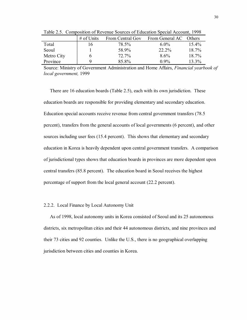
Table 2.5. Composition of Revenue Sources of Education Special Account, 1998 # of Units From Central Gov From General AC Others Total 16 78.5% 6.0% 15.4% Seoul 1 58.9% 22.2% 18.7% Metro City 6 72.7% 8.6% 18.7% Province 9 85.8% 0.9% 13.3% Source: Ministry of Government Administration and Home Affairs, Financial yearbook of local government, 1999

There are 16 education boards (Table 2.5), each with its own jurisdiction. These

education boards are responsible for providing elementary and secondary education.

Education special accounts receive revenue from central government transfers (78.5

percent), transfers from the general accounts of local governments (6 percent), and other

sources including user fees (15.4 percent). This shows that elementary and secondary

education in Korea is heavily dependent upon central government transfers. A comparison

of jurisdictional types shows that education boards in provinces are more dependent upon

central transfers (85.8 percent). The education board in Seoul receives the highest

percentage of support from the local general account (22.2 percent).

2.2.2. Local Finance by Local Autonomy Unit

As of 1998, local autonomy units in Korea consisted of Seoul and its 25 autonomous

districts, six metropolitan cities and their 44 autonomous districts, and nine provinces and

their 73 cities and 92 counties. Unlike the U.S., there is no geographical overlapping

jurisdiction between cities and counties in Korea.

31

Table 2.6. Local Autonomy Units in Korea (1998 and 1991) (* billion won) 1998 1991 Number of Units Expenditure* Percent Number of Units Expenditure* Percent

Total 250 67,469.4 100.0% 275 21,850.2 100.0%Seoul 26 11,133.1 16.5% 23 4,449.0 20.4% Head Office 1 8,216.0 12.2% 1 3,313.0 15.2% Autonomous 25 2,917.1 4.3% 22 1,136.0 5.2%Metro City 50 14,203.3 21.1% 39 4,153.4 19.0% Head Office 6 10,966.5 16.3% 5 3,012.3 13.8% Autonomous 44 3,236.8 4.8% 34 1,141.1 5.2%Province 9 15,044.5 22.3% 9 2,307.1 10.6%City 73 17,475.2 26.0% 67 5,418.8 24.8%County 92 9,613.4 14.2% 137 5,521.9 25.3%All accounts combined except education Source: Ministry of Government Administration and Home Affairs, Financial yearbook of local government, 1999 and 1992 Table 2.6 shows the number of local governments and their expenditures in 1998 and

1991. The number of local government units decreases from 275 in 1991 to 250 in 1998.

This decrease is largely due to city-county consolidations which were implemented during

the period 1995 through 1996. The major purpose of these consolidations was to increase

the size of local governments, thus making the fiscal capacity of local governments

stronger (Kwon, 1998:19).

The most interesting change is that, while the expenditure share of provinces has more

than doubled during this period, the expenditure shares of Seoul and county governments

have decreased. The decreasing expenditure share of counties may be explained partly by

the decrease in the number of county units. The increasing expenditure share of provinces

may indicate that the functional responsibility of provincial government is becoming

greater.

32

Table 2.7. Expenditure Shares of General, Enterprise Special, and other Special Account, 1998 (billion won) Total General Enterprise Other Special Expenditure % Expenditure % Expenditure % Expenditure % Total 67,469.5 100.0 51,520.6 76.4 7,188.1 10.7 8,819.0 13.1 Seoul 11,133.1 100.0 8,119.5 72.9 685.8 6.2 2,386.2 21.4 Head Office 8,216.0 100.0 5,400.7 65.7 685.8 8.3 2,187.9 26.6 Autonomous 2,917.1 100.0 2,718.8 93.2 0.0 0.0 198.3 6.8 Metro City 14,203.3 100.0 9,138.9 64.3 2,036.9 14.3 3,027.4 21.3 Head Office 10,966.5 100.0 6,175.3 56.3 2,036.9 18.6 2,754.3 25.1 Autonomous 3,236.8 100.0 2,963.6 91.6 0.0 0.0 273.1 8.4 Province 15,044.5 100.0 12,443.4 82.7 1,515.6 10.1 1,085.4 7.2 City 17,475.2 100.0 13,244.6 75.8 2,794.7 16.0 1,435.9 8.2 County 9,613.4 100.0 8,574.2 89.2 155.1 1.6 884.1 9.2 Source: Ministry of Government Administration and Home Affairs, Financial yearbook of local government, 1999

Table 2.7 shows the expenditure shares of general, enterprise special, and other special

accounts in relation to total expenditure for each jurisdictional type. Overall, the

percentages of general accounts are high. Especially, the general accounts of autonomous

districts in Seoul and other metropolitan cities have higher percentages (93.2 percent and

91.6 percent). The general accounts of head offices in Seoul and other metropolitan cities

have lower percentages (65.7 percent and 56.3 percent). Counties have the lowest

expenditure percentage for enterprise special accounts (1.6 percent). Autonomous

districts in Seoul and metropolitan cities do not have this type of account. For other

special accounts, head offices in Seoul and metropolitan cities have relatively high

percentages (26.6 percent and 25.1 percent).

This observation shows us that urban governments such as Seoul, other metropolitan

cities, and medium cities establish more special accounts in comparison with rural

33

governments such as counties. This may imply that urban governments provide more

diversified services to the residents than rural governments.

2.2.3. Local Revenues

Table 2.8. Composition of Local Revenues by Source (percentage) 1986 1987 1988 1989 1990 1991 1992 1993 1994 1995 1996 1997 1998

Own 71.5 68.6 73.0 73.4 75.9 75.4 78.5 76.9 76.4 75.5 76.3 76.3 72.1 Tax 27.1 27.5 30.0 38.8 30.8 30.8 29.7 31.9 32.4 32.1 29.5 28.4 26.6 Non 44.4 41.1 43.0 34.6 45.1 44.6 48.7 45.0 44.0 43.5 46.8 47.9 45.6 Grant 28.5 31.4 27.0 26.6 23.9 24.6 21.5 23.2 23.7 24.4 23.7 23.8 27.9 TOTAL 100 100 100 100 100 100 100 100 100 100 100 100 100 All local accounts are included except education Local borrowing excluded Source: Ministry of Government Administration and Home Affairs, Financial yearbook of local government, various years Korea�s local government revenues are composed of local taxes, non-tax revenues, and

grants such as local shared tax and subsidies. The total amount of local revenue has

increased from 7474.7 billion won in 1986 to 63327 billion won in 1998. This represents

a nine-fold increase. There are several interesting observations in Table 2.8. First, tax

revenue shares increased dramatically between 1986 and 1989 (27.1 percent to 38.8

percent), but it still has a relatively low share of the total local government revenues.

Second, overall the shares of non-tax revenues are high. Third, the shares of

intergovernmental grants steadily decreased from the late 1980s through the early 1990s

(28.5 percent to 21.5 percent) but by 1998 they returned to the late 1980s level. The

declining trend of intergovernmental grants share of total local government revenues is

due to the increase in non-tax revenue share of total local revenues. Since the end of

1997, Korea has suffered from a financial crisis that hit several Asian countries. That

34

financial collapse was one of the reasons for the increase in intergovernmental grants share

of total local revenues in order to supplement local tax revenue loss due to the economic

downturn.

Table 2.9. Composition of Local Revenue by Autonomy Unit, 1998 (billion won) Tax Share

(%) Non-Tax Share

(%) Grant Share

(%) Total Share

(%) Seoul 4,178.8 53.8 3,045.2 39.2 543.2 7.0 7,767.2 100.0Metro City 3,558.9 32.9 5,008.8 46.4 2,235.6 20.7 10,803.3 100.0Province 3,413.1 22.9 3,295.5 22.2 8,163.7 54.9 14,872.3 100.0 City 3,638.0 19.9 11,363.4 62.1 3,293.5 18.0 18,294.9 100.0 County 958.1 11.1 3,999.3 46.3 3,682.0 42.6 8,639.4 100.0 Autonomous 1,401.4 34.0 2,655.1 64.4 68.5 1.7 4,125.0 100.0 all accounts combined except education Source: Ministry of Government Administration and Home Affairs, Financial yearbook of local government, various years

As shown in Table 2.9, by the type of government, local governments have a different

revenue structure. Big cities and their autonomous districts have higher tax revenue

shares than other local governments. Autonomous districts and medium cities have non-

tax revenues as the most important revenue source. For province and county

governments, intergovernmental transfers are the most important revenue source. This

observation may imply that depending upon the type of local governments, the degree of

self-reliance rate is different. Because big cities have a larger tax base than rural cities and

counties, they have higher self-reliance rate. On the other hand, because rural cities and

counties do not have such a productive tax base, they are heavily dependent on

intergovernmental grants to finance their programs. In the following, tax revenue, non-tax

revenue, and intergovernmental grants are described in detail.

35

2.2.3.1. Local Tax

In general, there are six criteria to evaluate a tax: (1) economic efficiency, (2) fairness,

(3) administration, (4) revenue stability, (5) the link between spending and taxing, and (6)

tax visibility (Musgrave and Musgrave, 1989). First, economic efficiency tells us a tax

should minimally affect an economic decision because economic distortion induced by

taxes produces economic inefficiency. In other words, �the tax should ordinarily be

neutral: economic behavior should be the same with a particular tax in place as it would

have been without the tax� (Mikesell, 1995:294). For example, if jurisdiction A imposes a

tax on the consumption of cigarettes, consumers can purchase cigarettes in jurisdiction B

which imposes a lower tax. This involves an efficiency cost because individuals change

their behavior due to the tax-induced price changes. A simple solution for this situation is

that both of jurisdiction A and B impose the same tax rate on the consumption of

cigarettes. The uniform taxation across jurisdictions may reduce the efficiency cost related

to the mobility factor. However, the uniform taxation may be an impediment to efficiency

gain of fiscal decentralization because it may not allow local governments to provide the

tax and service packages that residents prefer.

Second, fairness is concerned with the concepts of horizontal and vertical equity.

Horizontal equity concerns equal treatment of taxpayers who have equal capability to pay

taxes. For example, suppose that two taxpayers are equivalent in income and wealth, but

one taxpayer pays a significantly greater tax. The tax structure would then lack horizontal

equity. On the other hand, vertical equity considers different treatments of taxpayers who

have different capabilities to pay taxes. Unlike the horizontal equity standard, there is

considerable disagreement as to what the proper differentiation should be. In general,

36

there are three types of tax burdens on income distribution: progressive, proportional, and

regressive. A progressive tax is one where the tax burden (as a percentage of income)

rises as income rises. People with higher income have higher marginal tax rates. A

proportional tax is one where the tax burden is constant as income rises. All people

regardless of their income have the same tax rate. A regressive tax is one where the tax

burden falls as income rises. People with higher income have lower marginal tax rates

even though the actual amount of tax contributions by people with higher income may

exceed that of people with lower income.

The conventional argument concerning tax assignment among levels of government

recommends that local governments should not use progressive taxation because of the

efficiency cost induced by the mobility factor. However, there is little empirical evidence

on this issue (e.g., Goodspeed, 1989; Mieszkowski and Toder, 1983). Rather, the

constraint on the local use of a specific tax, for example a progressive tax, may impede the

independent fiscal decision-making power in local governments. For example, if

jurisdiction A has considerable income variation among residents, and the mix of public

services and tax prices is not met by the demands of many residents in that people with

higher income want higher quality of services and people with lower income want a lower

tax price, one possible solution with the no mobility assumption might be to adopt a

progressive tax to finance higher quality services for the rich and to put a lower tax price

for the poor. In this sense, the proper choice of revenue instruments by local governments

may increase efficiency in resource allocation.

The third criterion is administrative simplicity. A tax should be collected at reasonable

cost because the cost of tax collection provides no net service to society (Mikesell,

37

1995:293). The collection cost, which consists of administrative cost and compliance cost

should be as low as possible. If a tax�s base and rate are complex, the collection cost will

be high. In practice, however, this criterion is reconciled with other objectives such as

efficiency and equity and becomes a complementary criterion. For example, a head tax

with a flat rate is the simplest tax base and rate to calculate but it may violate the equity

principle. As a result, it has not been adopted widely. Another example is a local property

tax. The property tax requires much more administrative complexity than other taxes such

as income and sales. Even though it is complex, local governments have adopted the

property tax due to other reasons such as efficiency. Therefore, this criterion should be

evaluated in conjunction with other objectives.

The fourth criterion is revenue stability. Citizens expect government to provide basic

public goods and services regardless of the condition of the private economy. Therefore,

a stable flow of tax revenue is important, especially in subnational governments because

subnational governments are more likely to suffer from economic downturn. One

indicator for revenue stability is revenue elasticity, which is the responsiveness of the tax

base with respect to income. If the revenue elasticity of a specific tax is relatively low, the

revenue flow of the tax is stable.

Fifth, the link between spending and taxing should be as clear as possible in subnational

governments. The link between spending and taxing cannot be always identified in a

public budget. Public economists suggest that benefit taxation may solve this difficulty. If

local governments adopt benefit taxation, people may be able to know how each program

spends the monies paid. Then voters can better evaluate public program options. This

38

will result in less tax resistance and avoidance behaviors because people receive services

they value.

Also, from the efficiency perspective, as mentioned earlier, there must be a

correspondence between the benefit zone of local public expenditure and the burden zone

of the tax. If there is tax exporting in which outsiders absorb part of the cost of local

services in a particular jurisdiction, the residents of the jurisdiction may not have to bear

the full cost of their own public services and, as a result, they have an incentive to push the

output of public services beyond the efficient level. This will result in inefficient resource

allocation.

In practice, however, extensive use of benefit taxation may face some difficulties. For

a benefit-base levy to be considered, there should be a strong link between the taxed

commodity and the public good being financed (e.g., the link between gasoline and

highway). But the link is not always explicit. Without an explicit link between the taxed

commodity and the public good financed, earmarked revenues do not contribute to

improve efficiency in resource allocation. Rather, they may impede the flexibility of local

budget operation.

Sixth, the degree of tax visibility depends on several factors: economic transaction,

size, and time (Bartlett, 1973). If the tax is part of the transaction, it is less visible. If the

payment is relatively small, the tax is less visible. If a tax is paid often, then it is less

visible.

According to several Korean scholars, there are several characteristics of the Korean

local tax system related to fiscal decentralization. First, the tax base and tax rate of local

governments are determined by national law and thus have the same structure across the

39

country. The central government gives local governments discretion to determine their

own tax rates within a limited range. Such taxes as inhabitant tax, automobile tax, city

planning tax, and regional development tax have a discretion range, but it is too narrow to

produce a different tax structure across the country (Kwon, 1998:82). The same tax

structure across the nation is obviously an impediment to fiscal decentralization because

local governments cannot readily respond to the demand change of local residents.

Second, local taxation relies heavily upon property-related taxes. In principle, property

taxes have the least revenue elasticity, which means the revenue flow is stable regardless

of economic fluctuations. In this sense, this revenue source is appropriate for local use.

However, Korean local governments levy taxes more heavily on sale and transfer of

properties than on possession of properties. The revenues from Acquisition and

Registration taxes far exceed those from Property and Aggregate Land taxes. Those

revenues from the sale and transfer of properties are likely to be sensitive to business

cycles in the property market. Therefore, revenue stability in Korean local governments is

not secure even though local taxation relies heavily on property-related taxes.

Third, the Korean local tax system incorporates a variety of tax expenditures9 set up by

the central government. In 1996, the tax expenditures amounted to more than 10 percent

of local tax revenues. The tax expenditure may encourage certain activities and assist

certain groups. The problem is that because the central government establishes tax

expenditures for local governments, certain tax expenditure items may not reflect well the

reality of those local governments. Rather, it undermines local revenue sources.

9 The tax expenditure is a revenue loss attributable to provisions of tax laws that allow a special exclusion, or deduction from gross income, or that provide a special credit, preferential tax rate, or deferral of tax liability (Mikesell, 1995:574).

40

Fourth, some scholars argue that local tax revenues are unevenly distributed between

urban and rural jurisdictions, and the regional inequality in revenue-raising capacity may be

a major obstacle to fiscal decentralization (e.g., Oh, 1992b). Ironically, however, the

uneven distribution of local revenue is actually what fiscal decentralization wants to

accomplish in terms of provision of various service/tax packages. Probably, the issue will

be that some portions of the nation cannot afford a so-called �minimum standard of public

services� due to weak revenue-raising capacity. However, regional disparities are not a

particular phenomenon in Korea. Regional disparities exist in most countries including

developed countries. A recent study shows that regional disparities in Korea are not as

severe as in US (Choi and Kwon, 1997). Therefore, the argument concerning regional

disparities seems to be somewhat exaggerated.

In 1998, the Korean local tax system was composed of 15 different taxes10 (refer to

Table 2.10). In 1986, it had 13 taxes. The 15 taxes may be classified into three broad

categories; taxes on income, taxes on property, and taxes on consumption. The share of

taxes on income decreased in 1990 to 10.8 percent from 17.2 percent in 1986, and

increased slightly afterwards, reaching 17.4 percent in 1998. The share of taxes on

property decreased in 1990 to 62.2 percent from 74.1 percent in 1986 and remained

relatively constant. The most dramatic change occurred in the share of taxes on

consumption. These taxes increased from 7.8 percent in 1986 to 26.2 percent in 1990.

This large increase in the share of taxes on consumption is due to the introduction of a

tobacco consumption tax in 1989.

10 Refer to Appendix A for a glossary of tax terms.

41

Table 2.10. Composition of Local Tax (billion won) 1986 Share

(%) 1990 Share

(%) 1995 Share

(%) 1998 Share

(%) Tax on Income 310.5 17.2 675.2 10.8 1,999.5 13.1 2,978.1 17.4 Inhabitant 227.7 12.6 529.8 8.5 1,701.4 11.1 2,639.1 15.4 Farmland Income 14.8 0.8 5.9 0.1 2.1 0.01 2.7 0.02 Business Firm 68.0 3.8 139.5 2.2 296.0 1.9 336.3 2.0 Tax on Property 1,340.5 74.1 3,875.8 62.2 10,508.2 68.6 11,007.2 64.2 Acquisition 371.2 20.5 1,164.9 18.7 2,691.0 17.6 2,479.8 14.5 Registration 395.9 21.9 1,377.6 22.1 3,632.5 23.7 3,388.5 19.8 Property 265.8 14.7 221.7 3.6 484.8 3.2 640.7 3.7 Automobile 139.1 7.7 413.5 6.6 1,545.2 10.1 2,174.6 12.7 Aggregate Land 0.0 0.0 381.9 6.1 1,235.2 801 1,199.3 7.0 City Planning 123.9 6.8 233.6 3.7 653.7 4.3 752.3 4.4 Fire Facility 44.6 2.5 82.6 1.3 0.0 0.0 0.0 0.0 Community Facility 0.0 0.0 0.0 0.0 204.4 1.3 301.7 1.8 Regional Development 0.0 0.0 0.0 0.0 61.1 0.4 70.3 0.4 Tax on Consumption 140.6 7.8 1,633.0 26.2 2,611.3 17.0 2,884.9 16.8 License 23.3 1.3 47.3 0.8 208.5 1.4 240.7 1.4 Butchery 18.6 1.0 17.3 0.3 33.9 0.2 48.2 0.3 Horse Race 9.4 0.5 57.9 0.9 217.0 1.4 329.4 1.9 Tobacco 89.3 4.9 1,510.5 24.2 2,151.9 14.0 2,266.6 13.2 Carry-over 18.2 1.0 46.0 0.7 197.8 1.3 278.1 1.6 Total Tax 1,809.8 100.0 6,230.0 100.0 15,316.8 100.0 17,148.3 100.0 Source: Ministry of Government Administration and Home Affairs, Financial yearbook of local government, various years

Overall, local tax revenues have been heavily dependent on property-related taxes but

consumption taxes are becoming an important revenue source. This means that the

Korean local governments tend to use more responsive taxes to economic fluctuations as a

revenue instrument. Even though responsive taxes may not be stable, they can generate

meaningful revenue during the periods of economic growth.

For individual taxes in 1998, the registration tax is the most important of all with a

share of 19.8 percent, followed by inhabitant tax (15.4 percent), acquisition tax (14.5

percent), tobacco tax (13.2 percent), and automobile tax (12.7 percent). The farmland tax

shows the lowest share of 0.02 percent. The registration tax status was changed from a

42

national to local tax in the 1976 Tax Reform Act. Its share has fluctuated around 20

percent. The inhabitant tax dropped below 10 percent in 1990 but climbed above 10

percent in 1995. The share of acquisition tax has shown a decreasing trend during the last

decade. The automobile tax has increased at a double-digit percentage since 1995. In

1985 the tobacco sales tax was initially incorporated in the local tax system and in 1989 its

tax base was expanded and it was renamed as the tobacco consumption tax. Before 1985

national monopoly profits from tobacco sales were transferred to the general account of

the central government. In 1989, this practice was repealed. Instead, the tobacco sales

tax became part of local tax base (Oh, 1992a:335).

Different types of local governments use different local taxes. Table 2.11 shows the

current usage of local tax instruments by the type of government (as of 1998). A main

characteristic of local tax usage by type of government is that there is little overlap in the

tax bases between the levels of government (i.e., between Seoul and other metropolitan

cities, and their autonomous districts; between provinces, and medium cities and counties).

While metropolitan cities including Seoul do not use property taxes, aggregate land taxes,

and business firm taxes, their sub-level governments, that is, autonomous districts use

them as revenue instruments. While medium city and county governments do not use

acquisition taxes, registration taxes, regional development taxes, license taxes, and horse

race taxes, their upper-level of governments, that is, provincial governments use them as

revenue instruments. Because national law determines the tax base, there may be few

overlapping tax assignments among the levels of government. Again, this may be good for

efficient tax administration, but centralized taxation may limit the independent fiscal

decision-making power in decentralized governments.

43

Table 2.11. Local Tax by the Type of Government (1998) Seoul & Metro Province Medium Cities Counties Autonomous Inhabitant O O O Farmland Income O O O Business Firm O O O Acquisition O O Registration O O Property O O O Automobile O O O Aggregate Land O O O City Planning O O O Community Facility O O O O Regional Develop O O License O O O Butchery O O O Horse Race O O Tobacco O O O Legend: o indicates the use of the tax. Source: Ministry of Government Administration and Home Affairs, Financial yearbook of local government, 1999

2.2.3.2. Non-Tax Revenue

Non-tax revenues include user charges, fees, interest earnings, sales of property,

carryover and so forth. Particular attention is paid to user charges and fees in the context

of fiscal decentralization. According to Zorn (1991:137), �User charges and fees are

payments for voluntarily purchased, publicly provided services that benefit specific

individuals, but exhibit public-good characteristics or are closely associated with public

goods.� In theory, user charges should be operated in the manner that an individual�s

charge depends both on benefit and cost of provision. In this way, public goods and

services can be produced and distributed using a private market mechanism rather than the

political budget process. Then user charges can play the role of private market prices. In

other words, they can provide clear demand signals. Then, a local government can

determine efficient level of services. However, if the prices of user charges are not

44

structured to reveal the true demand of a service (usually due to underpricing), user

charges are no longer an effective instrument for a clear demand signal.

Table 2.12. The Ratio of Earnings to Operating Costs in User-charge Items. Type of User Charge Item Earnings/Operating Costs Recreational Complex 56.2 Educational Facility 11.6 Cultural Facility 37.2 Business Facility 104.8 Public health Facility 33.1 Average 58.5 Source: Oh and Park (1996)

In Korea, as shown in Table 2.12, revenues from many user charges do not meet

operating expenses. The main reason for those deficits is due to the low rate of user

charges, which central mandates direct. National law requires that when local

governments set user-charge rates, they consult with the central bureau, which is more

concerned with price stability and inflation throughout the nation, than with local

government�s budget office. Also, central mandates require that local governments

provide certain services at no cost. Therefore, the current practice of central government

intervention on price setting on user charges may impede efficient resource allocation in

the local sector.

As shown in Table 2.8, the shares of non-tax revenue are high. This is because

enterprise and other special accounts as well as general accounts are included in Table 2.8.

Compared with the shares of non-tax revenue in general accounts only and all accounts

combined (Table 2.13), one may notice that the share of non-tax revenue in all accounts

combined (45.6 percent) is higher than the share in general accounts only (31.5 percent).

In comparing Korea to the U.S. non-tax revenues are 31.5 percent and 24.4 percent

45

respectively.11 Obviously, this comparison is rough but it gives us an idea of the heavy

dependence of Korean local revenue on non-tax sources.

Table 2.13. Composition of Local Revenues by Account, 1998 General account only All accounts combined Tax 35.0% 26.6% Non-Tax 31.5% 45.6% Grant 33.5% 27.9% Total 100.0% 100.0% Source: Ministry of Government Administration and Home Affairs, Financial yearbook of local government, 1999

However, there is a need for careful interpretation concerning the high share of non-tax

revenue. Non-tax revenue may be categorized as current non-tax revenue and temporary

non-tax revenue. The current non-tax revenue refers to the non-tax revenue which is

regularly collected in every fiscal year. Examples are user charges, fees, and interest

earnings. The temporary non-tax revenue refers to the non-tax revenue which is

temporarily gained in a particular fiscal year. Examples are sales of property and carry-

over.

11 Composition of revenue in state and local governments in the U.S.1995-1996 (State and Local Government Finances, 1995-1996) Revenue Share Tax 56.3% Non-tax 24.4% Grant 19.2%

46

Tabl

e 2.

14. C

ompo

sitio

n of

Non

-Tax

Rev

enue

(bill

ion

won

)

1986

19

87

1988

19

89

1990

19

91

1992

19

93

1994

19

95

1996

19

97

1998

Non

-Tax

91

6 87

5 1,

633

2,36

53,

980

5,57

26,

658

5,99

3 7,

738

5,41

013

,889

16,6

9215

,443

Shar

e (%

)

100.

0 10

0.0

100.

0 10

0.0

100.

0 10

0.0

100.

0 10

0.0

100.

0 10

0.0

100.

0 10

0.0

100.

0

C

urre

nt

245

271

280

358

503

660

751

766

1,08

61,

609

1,97

52,

383

2,17

0

Sh

are

(%)

26

.7

31.0

17

.115

.112

.611

.811

.312

.8

14.0

29.7

14.2

14.3

14.1

Te

mpo

rary

67

1 60

4 13

532,

007

3,47

74,

912

5,90

75,

227

6,65

23,

801

11,9

1414

,309

13,2

73

Sh

are

(%)

73.3

69

.0

82.9

84.9

87.4

88.2

88.7

87.2

86

.070

.385

.885

.785

.9

Car

ry-o

ver

323

394

942

1,31

52,

801

3,99

44,

912

4,22

9 5,

333

2,97

79,

804

12,2

4311

,293

Shar

e (%

) 35

.3

45.0

57

.755

.670

.471

.773

.870

.6

68.9

55.0

70.6

73.3

73.1

Gen

eral

acc

ount

onl

y So

urce

: Min

istry

of G

over

nmen

t Adm

inist

ratio

n an

d H

ome

Affa

irs, F

inan

cial

yea

rboo

k of

loca

l gov

ernm

ent,

vario

us y

ears

47

As shown in Table 2.14, the temporary non-tax revenue occupies a much bigger

portion of non-tax revenue than the current non-tax revenue, and the carry-over occupies

most of the temporary non-tax revenue. There may be several reasons why the carry-over

is so high in Korean local governments. First, because the central government transfers a

large amount of revenues near the end of fiscal year, local governments cannot make an

outlay of transfer revenues within the fiscal year. Unspent central transfers account for a

big portion of the carry-over. Second, in the case of a large-scale construction, the delay

of compensation agreements between local governments and property-owners may result

in carry-over. Third, the reason might be political. Before 1995 all executives of local

governments were appointed by the central government. The central government used to

evaluate the appointed executives by the figures in budget sheet. They were criticized for

running a deficit budget and they were praised for running a budget surplus. Therefore,

local executives tend to have a conservative budgeting strategy in order to avoid deficits in

the budget sheet. This budgetary practice also may contribute to a high level of carry-

over. As a result, the real share of own-source revenue might be much lower than the

figures presented in Table 2.8 because non-tax revenue actually includes transfer revenues

from the past year.

2.2.3.3. Intergovernmental Grants

There are several purposes for intergovernmental grants. First, they may reduce

vertical fiscal imbalance between the central and local governments. Second, they may

alleviate horizontal imbalance among local governments. Third, they may internalize

externalities so as to improve efficiency in resource allocation. There are three types of

48

intergovernmental grant systems from the central to local governments in Korea: local

share tax, subsidies, and local tax transfer. The local share tax is similar to general

revenue sharing in the United States. The size of the grant is determined by a formula and

the central government does not attach provisions on the local governments� use of the

funds. Subsidies are provided under the condition that they should be used for a specific

purpose. The local tax transfer is different from the local share tax in that the central

government attaches provisions, while no such provisions are attached to the local share

tax. It is also different from national subsidies in that not only are the financial sources of

the grant limited to some fixed percent of three specific taxes, but also provisions attached

are looser than those on the national subsidies. Later on, these three types of

intergovernmental grant systems are described in detail.

Table 2.15. Share of Intergovernmental Revenues to Total Local Revenues (percentage) 1986 1987 1988 1989 1990 1991 1992 1993 1994 1995 1996 1997 1998

Intergovern 28.5 31.4 27.0 26.6 23.9 24.6 21.5 23.2 23.7 24.4 23.7 23.8 27.9 Share Tax 19.4 19.5 16.5 14.6 13.4 13.2 12.3 12.8 11.9 11.9 10.8 10.5 10.9 Subsidies 9.2 11.9 10.5 11.7 10.3 9.2 5.4 6.2 7.7 8.6 8.3 8.5 12.0 Transfer 0.0 0.0 0.0 0.0 0.0 2.2 3.8 4.2 4.1 4.0 4.4 4.5 4.5 Others 0.0 0.0 0.0 0.0 0.2 0.0 0.0 0.0 0.0 0.0 0.2 0.3 0.4 Own-Source 71.5 68.6 73.0 73.4 75.9 75.4 78.5 76.9 76.4 75.5 76.3 76.3 72.1 Total 100 100 100 100 100 100 100 100 100 100 100 100 100 All accounts combined except education special account Local borrowing is excluded from own-source revenue Source: Ministry of Government Administration and Home Affairs, Financial yearbook of local government, various years

Table 2.15 shows how local dependence upon intergovernmental revenues has changed

between 1986 and 1998. The percentage of local share tax that has occupied the largest

portion of intergovernmental revenues has somewhat decreased. The share of subsidies is

49

fluctuating. Local tax transfer, which has been implemented since 1991, is becoming an

important revenue source of local governments.

Table 2.16. Composition of Intergovernmental Grants by Autonomy Units, 1998 (billion won) Share Tax Share

(%) Subsidies Share

(%) Tax Transfer

Share (%)

Others Share (%)

Total Share (%)

Seoul 3.1 0.6 540.1 99.4 0.0 0.0 0.0 0.0 543.2 100.0 Metro City 181.9 8.1 1,714.1 76.7 320.5 14.3 19.1 0.9 2,235.6 100.0 Province 1,488.2 18.2 5,415.1 66.3 993.7 12.2 266.7 3.3 8,163.7 100.0 City 2,446.0 74.3 40.1 1.2 801.7 24.3 5.7 0.2 3,293.5 100.0 County 2,888.0 78.4 21.9 0.6 768.6 20.9 3.5 0.1 3,682.0 100.0 Autonom 32.4 47.3 35.1 51.2 1.0 1.5 0.0 0.0 68.5 100.0 all accounts combined except education Source: Ministry of Government Administration and Home Affairs, Financial yearbook of local government, 1999

Table 2.16 shows the composition of intergovernmental grants by local governments.

Different types of local governments have varying compositions of intergovernmental

grants as a revenue source. Counties and medium cities have higher percentages of local

share tax revenue than other sources of intergovernmental revenue. Seoul, other

metropolitan cities, and province governments have higher shares of national subsidies

than other intergovernmental grants. Most interestingly, while national subsidies are not a

very important intergovernmental revenue source in medium cities and counties, local tax

transfer funds occupy a significant portion of intergovernmental revenues in medium cities

and counties. In the following, each type of intergovernmental revenue is described in

detail.

50

Local Share Tax12

The local share tax is similar to general revenue sharing in the United States. The size

of the grant is determined by a formula and the central government does not attach

provisions on the local governments� use of the funds.

The local share tax mainly has two purposes. First, it may reduce the vertical fiscal

imbalance between the central government and local governments. Second, it may

alleviate horizontal fiscal imbalance, or fiscal inequality, among local governments. Since

the wealth of different regions and their potential tax bases differ markedly, the central

government engages in regional distribution of local share tax, providing more to poorer

regions.

Under the current local share tax system defined by the Local Share Tax Law, 13.27

percent of the revenues from domestic taxes of the central government are sources for the

local share tax with 10/11 of the total fund going to ordinary local share tax and the

remaining 1/11 to special local share tax. The percentage (13.27 percent) itself is not

based on certain theoretical ground, but it was an outcome of political compromise.13 The

Ministry of Government Administration and Home Affairs is responsible for allocating

funds to the various local governments. The amount of ordinary local share tax is based

on a budget deficit concept, i.e., the difference between basic financial demand (need) and

basic financial revenue (ability). The amount of special local share tax is based on special

12 It is also called local share grant from the perspective of the central government. However, from the perspective of local governments, it is local tax that the central government collects for local governments. 13 Before 1972, 17.6% of domestic taxes were to be set aside to fund this program. During the periods of 1972 and 1982, the legally mandated set-aside system was eliminated. The program was funded on ad hoc basis. After 1982, 13.27% of domestic taxes have been set aside to fund this program.

51

contingency of local governments such as natural disaster or special need for construction

or maintenance of city hall or social welfare facility.

The ordinary local share tax reimburses local governments in the amount of the

difference between the cost of an estimated standard of public services and the revenue

yield from a standard of tax effort. If a local government has more standardized revenue

than standardized expenditure, no local share tax fund is allocated to that jurisdiction. The

measurement procedure of the cost of an estimated standard of public services and the

revenue yield from a standard of tax effort is prescribed in the Local Share Tax Law.

For the measurement of the cost of an estimated standard of public services, the law

specifies 28 expenditure items to be measured and their unit of measurement.14 The unit

cost to apply for the measurement is differentiated depending on the type of local

government such as Seoul, metropolitan city, province, medium city, and county. But the

same type of local government is assumed to have uniform unit costs for a certain service.

For example, all metropolitan cities have the same unit cost for a certain service, all

provinces do the same, all medium cities do the same, and all counties do the same.

Assigning uniform unit costs across the same type of local government may not be

reasonable because each local jurisdiction may not actually pay the same unit cost for the

same service. Therefore, a coefficient of correction is employed to correct the

measurement error induced by the assignment of uniform unit cost. Then, the

standardized cost for jurisdiction is calculated as, first, multiplying the unit of

measurement by the unit cost and the coefficient of correction, and then summing all 28

standardized costs.

14 Appendix B includes a hypothetical example of calculation of the standardized cost in A city.

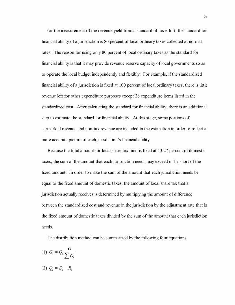
52

For the measurement of the revenue yield from a standard of tax effort, the standard for

financial ability of a jurisdiction is 80 percent of local ordinary taxes collected at normal

rates. The reason for using only 80 percent of local ordinary taxes as the standard for

financial ability is that it may provide revenue reserve capacity of local governments so as

to operate the local budget independently and flexibly. For example, if the standardized

financial ability of a jurisdiction is fixed at 100 percent of local ordinary taxes, there is little

revenue left for other expenditure purposes except 28 expenditure items listed in the

standardized cost. After calculating the standard for financial ability, there is an additional

step to estimate the standard for financial ability. At this stage, some portions of

earmarked revenue and non-tax revenue are included in the estimation in order to reflect a

more accurate picture of each jurisdiction�s financial ability.

Because the total amount for local share tax fund is fixed at 13.27 percent of domestic

taxes, the sum of the amount that each jurisdiction needs may exceed or be short of the

fixed amount. In order to make the sum of the amount that each jurisdiction needs be

equal to the fixed amount of domestic taxes, the amount of local share tax that a

jurisdiction actually receives is determined by multiplying the amount of difference

between the standardized cost and revenue in the jurisdiction by the adjustment rate that is

the fixed amount of domestic taxes divided by the sum of the amount that each jurisdiction

needs.

The distribution method can be summarized by the following four equations.

(1) G QGQi i

i

=∑

(2) Q D Ri i i= −

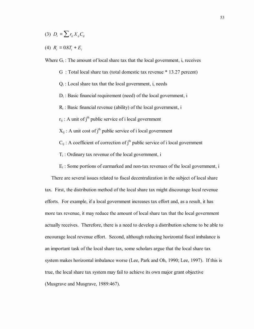
53

(3) D r X Ci ij ij ij=∑

(4) R T Ei i i= +08.

Where Gi : The amount of local share tax that the local government, i, receives

G : Total local share tax (total domestic tax revenue * 13.27 percent)

Qi : Local share tax that the local government, i, needs

Di : Basic financial requirement (need) of the local government, i

Ri : Basic financial revenue (ability) of the local government, i

rij : A unit of jth public service of i local government

Xij : A unit cost of jth public service of i local government

Cij : A coefficient of correction of jth public service of i local government

Ti : Ordinary tax revenue of the local government, i

Ei : Some portions of earmarked and non-tax revenues of the local government, i

There are several issues related to fiscal decentralization in the subject of local share

tax. First, the distribution method of the local share tax might discourage local revenue

efforts. For example, if a local government increases tax effort and, as a result, it has

more tax revenue, it may reduce the amount of local share tax that the local government

actually receives. Therefore, there is a need to develop a distribution scheme to be able to

encourage local revenue effort. Second, although reducing horizontal fiscal imbalance is

an important task of the local share tax, some scholars argue that the local share tax

system makes horizontal imbalance worse (Lee, Park and Oh, 1990; Lee, 1997). If this is

true, the local share tax system may fail to achieve its own major grant objective

(Musgrave and Musgrave, 1989:467).

54

Subsidies

Subsidies are usually provided under the condition that they should be used for a

specific purpose. There are two types of subsidies depending on whether the objective is

national or local. First, there are projects to maintain and provide for a national minimum

level of service. Very often, some local governments have difficulty in providing a

national minimum level of public service due to their limited resources. This causes many

problems, such as resident migration to urban areas, which further deteriorate the local

government�s financial capability. For projects of this type, the central government

provides the subsidies, but delegates its implementation power to local governments since

they can potentially carry out those projects more efficiently and conveniently. Subsidies

for social security and the development of agriculture and fisheries are examples. The

other kinds of subsidies are related to local level projects whose benefits may exceed the

local jurisdiction. These are used to encourage spending on certain public services for

each local government. Without the subsidies, local governments may tend to

underproduce the public services. Therefore, the central government requires that the

local governments spend subsidies only on specific services which might be

underproduced otherwise. Examples include subsidies for city hospitals and construction

of a local subway. In both cases, according to the government, the localities should spend

the subsidy monies only on the purpose specified in the program.

The various ministries administer the subsidy programs. The Ministries of Agriculture

and Fisheries, Transportation, Health and Social Affairs, Construction, and Industries and

Commerce are major players in the allocation of national subsidies. Local governments

which want to receive the subsidies to finance certain programs must apply for the monies

55

to the program-related ministry. The central ministry which receives the subsidy

application has all power to approve, disapprove, or revise the application. If the

application is approved, the ministry must secure funds from the Ministry of Finance and

Economy and consult with the Ministry of Government Administration and Home Affairs.

In the distribution of national subsidies, the ad hoc decision-making of the central

government plays a major role. For example, usually subsidies have a matching

requirement and the matching rates are determined at the central government�s discretion.

Therefore, depending on the central government�s decision, some programs have lower

matching rates while others have higher matching rates. In other words, there is no

specific guideline for the distribution of national subsidies. Instead, the central

government�s policy judgements are the determinants.

There is an irony between fiscal decentralization and subsidies. As fiscal

decentralization proceeds, local governments may take more functional responsibilities

which were once the central government�s tasks. As a result, local governments are likely

to encounter more situations in which they must deal with externalities. An efficient

solution may be to finance those programs by a categorical matching grant such as the

national subsidies. However, heavy dependence on national subsidies may impede fiscal

discretion of local governments.

Local Tax Transfer

In 1991, local tax transfers were introduced to strengthen the revenue-raising capacity

of local governments and to ensure a more balanced regional development.

56

The local tax transfer is different from the local share tax in that the central government

attaches provisions, while no such provisions are attached to the local share tax. It is also

different from national subsidies in that not only are the financial sources of the grant

limited to some fixed percent of three specific taxes, but also provisions attached are

looser than those on the national subsidies.

Also, the local tax transfer is similar to the national subsidies in that the main purpose

of the local tax transfer is to deal with externalities. It is also similar to the local share tax

in that it may allow local governments to have fiscal discretion. Therefore, this

intergovernmental grant system makes an effort to solve the incongruity between fiscal

decentralization and categorical matching grant mentioned before.

The choice of targeted programs financed by the local tax transfer is in the hands of the

central government. In 1991, this fund was allocated only to the projects related to local

road maintenance but since then the central government has added three other projects to

the targeted programs: regional development of the agrarian and fishing villages, water

pollution prevention, and youth upbringing. Within the purposes of those projects, local

governments may have considerable discretion concerning how to spend the monies. The

local tax transfer funds are distributed according to a standard developed by the central

government. In order to apply the standard, local governments should submit necessary

information related to the targeted programs to the Ministry of Administration and Home

Affairs and the related ministries. Then, depending on the information submitted, each

local government receives the local tax transfer fund.

One of the problems in the implementation of the local tax transfer is related to the

selection of the targeted programs. If the targeted programs are specified in too detailed a

57

manner, it will be the same as the subsidies. Therefore, broader definition of the programs

is needed to increase local discretion.

Other Types of Grant

Besides the three major types of intergovernmental grants, there are additional three

grant systems implemented in Korea; increased amount share grant, control grant, and city

and provincial subsidies. The increased amount share grant has characteristics that

supplement the local share tax. It is granted when local governments face urgent and

special contingencies such as a flood. The control grant and city and provincial subsidies

are local-to-local grants. Seoul and other metropolitan cities provide control grants for

their autonomous districts. The main purpose of this grant is to relieve fiscal discrepancies

among autonomous districts. The city and provincial subsidies have the same purpose as

the national subsidies. Seoul, metropolitan cities, and provincial governments grant them

to autonomous districts, cities, and counties.

2.2.3.4. Summary

We reviewed the revenue structure of local government in Korea. Korea�s local

government revenues are composed of local taxes, non-tax revenues, and

intergovernmental grants. There are several characteristics of the local revenue system

related to fiscal decentralization. First, the tax base and tax rate have almost the same

structure across the country. This may be an impediment to fiscal decentralization

because local governments cannot readily respond to the demand change of local

residents. Second, tax revenue has a relatively low share of total local government

58

revenues. This implies that local governments in Korea may have a low revenue-raising

capability. Third, local tax revenues have been heavily dependent on property-related

taxes but consumption taxes are becoming an important revenue source. Even though

responsive taxes such as consumption taxes may not be stable, they can generate

meaningful revenue during the periods of economic growth. Fourth, unconditional grants

such as the local share tax, which has been a major source of financing local public goods

and services, has been steadily declining since the late 1980s.

2.2.4. Local Expenditures

The functional classification of local expenditure shows what functions local

governments actually perform. According to Financial Yearbook of Local Government,

there are seven functional classifications of local expenditures; (1) General Administration,

(2) Social Welfare, (3) Industry and Economy, (4) Regional Development, (5) Culture and

Physical Education, (6) Civil Defense, and (7) Support and Others.15

General Administration expenditures are the expenses related to general administration,

legislation and elections in local governments. Social Welfare expenditures include

welfare, public health, and sanitation. Industry and Economy expenditures are the

spending related to agriculture and fishery development (e.g., farmland rearrangement),

development of natural resources, tourism, and transportation. Regional Development

15 Until 1985, the functional classifications included (1) general administration, (2) social welfare, (3) industry and economy, (4) public works, (5) civil defense, and (6) support and other. After 1985 civilization and physical education expenditure item was added in the classification and public works item was renamed as regional development. In 1989, National assembly expenditure item was added and thus, there were 8 functional classifications. From 1996, again, there was re-classification of functions. Social welfare, industry and economy, regional development, and culture and physical education were consolidated into two functional classifications, that is, social development and economic development. These frequent changes in functional classifications may make data collection difficult.

59

expenditures include local infrastructure investment such as roads and bridges, and

housing and community development. Culture and Physical Education expenditures

include cultural property management and physical education. Civil Defense expenditures

include civil defense facilities and fire fighting. Support and Other expenditures include

local borrowing repayment, transfers, contingency, and miscellaneous expenses.

Compared with functional assignment of state and local expenditures in the U.S.,

Korea�s functional classification does not have elementary and secondary education and

police expenditures. As mentioned earlier, because the education special account is

heavily dependent upon central transfers and operated independently from general

government operations, the expenditures of education are excluded in this functional

classification. Also, unlike the U.S., public safety such as police protection is a function of

the central government.

Table 2.17. Functional Classification of Local Expenditure by Account, 1995 (billion won) Total General Account Special Account*

Expenditure (%) Expenditure (%) Expenditure (%)

General Administration 7,641.6 15.4 7,630.4 21.3 11.2 0.1Social Welfare 6,369.2 12.8 5,268.6 14.7 1,100.6 7.9Industry & Economy 7,067.1 14.2 6,378.0 17.8 689.2 4.9Regional Development 22,187.7 44.6 10,231.5 28.6 11,956.3 85.5Culture & Physical Edu 2,090.2 4.2 2,031.5 5.7 59.1 0.4Civil Defense 643.0 1.3 643.0 1.8 0.0 0.0Support & Others 3,783.6 7.6 3,609.2 10.1 174.4 1.2Total 49,782.4 100.0 35,791.9 100.0 13,990.8 100.0* Education special account excluded Source: Ministry of Government Administration and Home Affairs, Financial yearbook of local government, 1996

Table 2.17 shows the structure of local expenditures in Korea. Out of all local

government expenditures, Regional Development is the highest, followed by General

60

Administration, Industry and Economy, and Social Welfare. However, considering the

general accounts only, one can find the share of Regional Development decreases

dramatically. The reason is that local special accounts are composed of many public

works related accounts such as water and sewage which are related directly to the regional

development function.

The fact that Regional Development occupies a high portion of local government

expenditures indicates local governments are actively involved in constructing local

infrastructure. Several Korean scholars argue that General Administration occupies too

large a portion of government expenditure in comparison with Japan (11.1 percent) and

U.S. (4.0 percent) (Kim, 1997:52-53).

Table 2.18. Functional Classification of Local Expenditure by Government Unit, 1995 (billion won) Seoul* Metro* Province City County Exp. (%) Exp. (%) Exp. (%) Exp. (%) Exp. (%) General 1,200.9 22.3 1,336.0 19.8 710.0 8.0 2,491.2 29.5 1,892.2 29.6 Social W 908.0 16.8 1,224.9 18.2 1,005.6 11.4 1,349.1 16.0 780.9 12.2 Indu&Ec 73.3 1.4 263.2 3.9 2,994.0 33.9 1,127.4 13.4 1,920.1 30.1 Regional 1,652.9 30.7 2,078.1 30.8 2,155.3 24.4 2,849.2 33.8 1,495.9 23.4 Culture 548.0 10.2 491.8 7.3 332.1 3.8 455.4 5.4 203.8 3.2 Civil D 137.2 2.5 136.0 2.0 325.8 3.7 21.1 0.3 22.9 0.4 Support& 871.2 16.2 1,210.5 18.0 1,316.2 14.9 139.7 1.7 71.6 1.1 Total 5,391.5 100.0 6,740.5 100.0 8,839.0 100.0 8,433.1 100.0 6,387.4 100.0 General account only * including autonomous districts Source: Ministry of Government Administration and Home Affairs, Financial yearbook of local government, 1996

Table 2.18 shows functional shares of local expenditure by governmental unit in 1995.

Provincial governments have an unusually low share of General Administration (8.0

percent) in comparison with other governmental units. Small governments such as

61

medium cities and counties have relatively high shares of General Administration

(respectively 29.5 percent and 29.6 percent) in comparison with big cities. Provincial and

county governments have the least share of Social Welfare spending (respectively 11.4

percent and 12.2 percent). Metropolitan cities such as Seoul have low shares of Industry

and Economy expenditures. This is because Industry and Economy expenditures in Korea

are mainly related to economic growth in rural areas. For Regional Development

expenditures, medium cities have the highest share (33.8 percent), followed by

metropolitan cities (30.8 percent) and Seoul (30.7 percent). Provincial and county

governments have relatively low shares 24.4 percent and 23.4 percent respectively.

Another interesting observation is that big cities have high shares of Support and Other

expenditures compared with medium cities and counties.

Table 2.19 shows the local expenditure share changes from 1986 to 1995. General

Administration shows a relatively high portion of local expenditures notably decreasing

from 22.1 percent in 1986 to 18.0 percent in 1991 and increasing to 21.3 percent in 1995.

Social Welfare shows a relatively stable pattern fluctuating around 15 percent. Industry

and Economy steadily decreases from 14.7 percent in 1986 to 12.1 percent in 1991 and

fluctuating thereafter. Regional Development increases dramatically from 28.1 percent in

1986 to 37.8 percent in 1991, and then decreases to 28.6 percent in 1995.

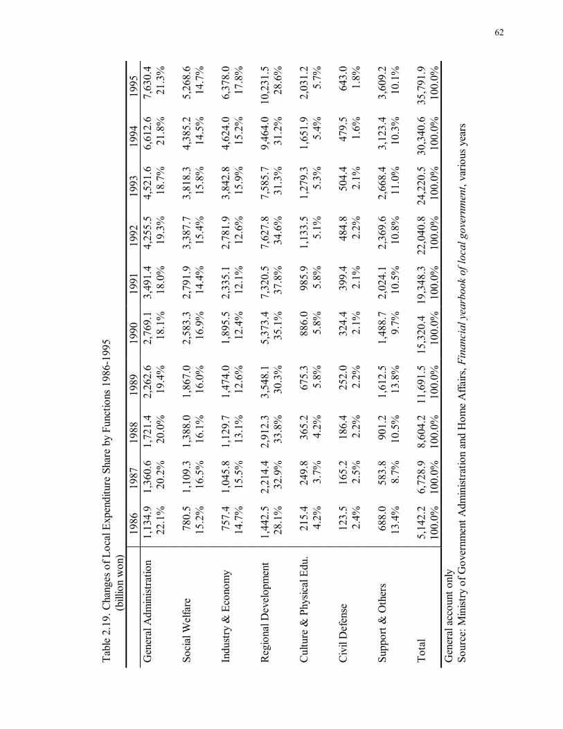
62

Tabl

e 2.

19. C

hang

es o

f Loc

al E

xpen

ditu

re S

hare

by

Func

tions

198

6-19

95

(bill

ion

won

)

1986

19

87

1988

19

89

1990

19

91

1992

19

93

1994

19

95

Gen

eral

Adm

inist

ratio

n 1,

134.

9 1,

360.

61,

721.

42,

262.

62,

769.

13,

491.

44,

255.

54,

521.

66,

612.

67,

630.

4

22.1

%

20.2

%20

.0%

19.4

%18

.1%

18.0

%19

.3%

18.7

%21

.8%

21.3

%

So

cial

Wel

fare

78

0.5

1,10

9.3

1,38

8.0

1,86

7.0

2,58

3.3

2,79

1.9

3,38

7.7

3,81

8.3

4,38

5.2

5,26

8.6

15

.2%

16

.5%

16.1

%16

.0%

16.9

%14

.4%

15.4

%15

.8%

14.5

%14

.7%

Indu

stry

& E

cono

my

757.

4 1,

045.

81,

129.

71,

474.

01,

895.

52,

335.

12,

781.

93,

842.

84,

624.

06,

378.

0

14.7

%

15.5

%13

.1%

12.6

%12

.4%

12.1

%12

.6%

15.9

%15

.2%

17.8

%

R

egio

nal D

evel

opm

ent

1,44

2.5

2,21

4.4

2,91

2.3

3,54

8.1

5,37

3.4

7,32

0.5

7,62

7.8

7,58

5.7

9,46

4.0

10,2

31.5

28

.1%

32

.9%

33.8

%30

.3%

35.1

%37

.8%

34.6

%31

.3%

31.2

%28

.6%

Cul

ture

& P

hysic

al E

du.

215.

4 24

9.8

365.

267

5.3

886.

098

5.9

1,13

3.5

1,27

9.3

1,65

1.9

2,03

1.2

4.

2%

3.7%

4.2%

5.8%

5.8%

5.8%

5.1%

5.3%

5.4%

5.7%

Civ

il D

efen

se

123.

5 16

5.2

186.

425

2.0

324.

439

9.4

484.

850

4.4

479.

564

3.0

2.

4%

2.5%

2.2%

2.2%

2.1%

2.1%

2.2%

2.1%

1.6%

1.8%

Supp

ort &

Oth

ers

688.

0 58

3.8

901.

21,

612.

51,

488.

72,

024.

12,

369.

62,

668.

43,

123.

43,

609.

2

13.4

%

8.7%

10.5

%13

.8%

9.7%

10.5

%10

.8%

11.0

%10

.3%

10.1

%

To

tal

5,14

2.2

6,72

8.9

8,60

4.2

11,6

91.5

15,3

20.4

19,3

48.3

22,0

40.8

24,2

20.5

30,3

40.6

35,7

91.9

10

0.0%

10

0.0%

10

0.0%

10

0.0%

10

0.0%

10

0.0%

10

0.0%

10

0.0%

10

0.0%

10

0.0%

G

ener

al a

ccou

nt o

nly

Sour

ce: M

inist

ry o

f Gov

ernm

ent A

dmin

istra

tion

and

Hom

e A

ffairs

, Fin

anci

al y

earb

ook

of lo

cal g

over

nmen

t, va

rious

yea

rs

63

To summarize, two large portions of general account expenditures are Regional

Development and General Administration. This is because local governments are involved

actively in constructing local infrastructure. Comparing the functional classification of

local expenditure by the type of governmental unit, we find that there are some variations

between urban and rural governments, and between big and small governments. During

the periods of 1986 and 1995 each functional expenditure share is fluctuating. These

observations show that in recent years local public finance in Korea has changed a great

deal.

2.3. Summary

The first part of this chapter described the recent development of local autonomy and

fiscal decentralization, and defined the concept of fiscal decentralization. The latter part

of this chapter describes the fiscal structure of local government in Korea. As of 1998,

local autonomy units in Korea consisted of Seoul and its 25 autonomous districts, six

metropolitan cities and their 44 autonomous districts, and nine provinces and their 73

cities and 92 counties. Korea�s local government revenues are composed of local taxes,

non-tax revenues, and intergovernmental grants. Tax revenue has a relatively low share of

total local government revenues, while the shares of non-tax revenues are high. Local tax

revenues are unevenly distributed between urban and rural jurisdictions. As a result, rural

jurisdictions are heavily dependent on intergovernmental grants to finance their programs.

There is a need for careful interpretation concerning the high share of non-tax revenue

in that non-tax revenue actually includes transfer revenues from the past year. There are

64

three types of intergovernmental grant systems from the central to local governments in

Korea: local share tax, subsidies, and local tax transfer.

Out of all local government expenditures, Regional Development is the most important

expenditure, followed by General Administration, Industry and Economy, and Social

Welfare. This means local governments in Korea are actively involved in local

infrastructure. Comparing functional classifications of local expenditure by the type of

governmental unit, we find that there are some variations between urban and rural

governments, and between big and small governments.

During the periods of the late 1980s and 1990s, fiscal decentralization policies have

been implemented in Korea. During that time, local finance in Korea has changed a great

deal. However, we may not be able to identify the effects of fiscal decentralization on

local finance through descriptive analysis alone. In the next chapter, research hypotheses

are formulated to systematically analyze the effects of decentralization on local public

finance in Korea.

65

CHAPTER 3

HYPOTHESES AND LITERATURE REVIEW In the previous chapter, we conducted a descriptive analysis of fiscal decentralization�s

effects on local finance. In this chapter, research hypotheses are formulated to

systematically analyze the effects of decentralization on local public finance in Korea. In

the first section, we develop a modified version of Brennan and Buchanan�s

decentralization hypothesis to test the effects of fiscal decentralization on the size of the

public budget. In the second section, we present two hypotheses concerning functional

realignment. In the third section, we formulate a hypothesis regarding decentralization�s

effect on fiscal independence of local governments.

3.1. The Effect of Decentralization on the Size of Public Budget

3.1.1. Fiscal Decentralization and Efficiency

A decentralized system is expected to respond better to local preferences and needs,

and to promote competition among local units in the provision of public goods and

services. Efficiency is improved as adjusting supply to demand. Earlier, we presented the

theoretical argument that showed how decentralized provision of public services could

minimize the welfare loss from the centralized provision of public services (Oates, 1977).

Oates and Schwab (1991) also show that interjurisdictional competition fosters efficiency.

These scholars (1991:140-141) argue that under the assumption that taxes play the same

role as prices, �the outcome under interjurisdictional competition is identical to the

outcome that would emerge if one were to replace local governments with perfectly

66

competitive firms that supplied local public goods to firms and households at marginal

cost.�

This view on government decentralization and competition is the opposite of the

traditional one. The classical administrative view on government fragmentation is that it

causes uncoordinated service delivery (Bollens, 1957), loss of economies of scale (ACIR,

1964), deterioration of accessibility and accountability (Glendening, 1984), and private

interests making key public decisions (Perrenod, 1984).

Also, the literature on intergovernmental relations used to pay attention to cooperation

among levels of governments (e.g., Grodzins, 1966) while it paid little attention to

competition among the same levels of government. Traditionally, public economists also

argued that interjurisdictional competition to retain and attract residents and businesses

was at best a zero-sum game (Kenyon and Kincaid, 1991:2).

From both sides, however, the promised benefits or costs of decentralized provision of

goods and services are usually based on theoretical arguments. A major obstacle to

measuring efficiency gain directly is that we may encounter tremendous difficulties in

measuring units of public output and in obtaining reliable estimates of individual demand

functions, both of which are the necessities for direct measurement. Despite this difficulty,

some empirical studies have tried to measure directly whether or not efficiency gains from

decentralized provision is realized in the real world (e.g., Bradford and Oates, 1974).

However, their study area is limited to one specific service (education) and a small

geographical area (northeastern New Jersey). Therefore, their direct measure of efficiency

gains from the decentralization provision of public finance does not fit our purpose

67

because we want to evaluate the overall performance of the public sector in Korea, not a

specific service in a limited geographical area.

There may be an alternative approach to the measurement of the expected benefits of

decentralized provision in an empirical setting. In this sense, we borrow Brennan and

Buchanan�s decentralization hypothesis to test the effects of fiscal decentralization on the

Korean public sector. Brennan and Buchanan (1980) assume government as �Leviathan�

which �systematically seeks to exploit its citizenry through the maximization of the tax

revenues that it extracts from the economy� (Oates, 1985:748). Their view on

government is drawn from the economics literature of industrial organizations (Joulfaian

and Marlow, 1990). If a firm is the sole source of supply for a certain commodity, it could

set its price at higher levels than would be the case if many competing sellers served the

market. The common solution to monopoly power is to allow competition among firms,

which will eliminate monopoly power and result in essentially competitive prices and

outcomes. Brennan and Buchanan analogize government as a firm with monopoly power

and suggest that a monolithic government can be constrained by decentralizing taxes and

expenditures that will promote competition among subnational governments. That

competition makes each decentralized government impose taxes on residents and

businesses strictly in terms of their relative public goods evaluations in order to retain and

attract residents and businesses. Therefore, this outcome will be efficient and the lower

tax burden will collectively decrease the size of the public budget. Following this logic,

we might argue that fiscal decentralization decreases the size of public budget.

This argument is basically the same as the conventional fiscal decentralization theory in

that the better fitted service/tax package can improve efficiency in resource allocation.

68

However, it is quite different in that it does not assume government fiscal decisions

automatically follow the demand function of citizens. In other words, it discards the

presumption of a benevolent and public welfare-maximizing government. In particular,

this hypothesis invalidates the conventional median voter model. However, the fact that it

discards the median voter model makes this hypothesis most attractive in studying fiscal

decentralization in developing countries. In developing countries, there may be no voters

to reveal their preferences in the local sector. Even in cases where voter�s preferences are

revealed, local officials may not act immediately according to the voter�s preferences

because of a long tradition of centralization or institutional barriers such as limited taxing

and spending power. Another advantage of using this hypothesis is that it provides

empirically testable hypotheses.

However, there are some qualifications when we are testing the decentralization

hypothesis in Korea. First, we cannot relate directly the lower tax burden to the size of

budget as Oates (1985) did. Because demand for public services will increase as price

decreases, we are not sure whether or not the total government receipt of tax monies

decreases after the tax burden changes. However, we can assume that the total

government receipt of tax monies will decrease after a lower tax burden in that local

public goods are relatively price inelastic; that is, quantity is insensitive to price change.

Second, in order for decentralized governments to behave like private firms, there should

be a sufficient number of decentralized governments which compete with one another to

retain and attract residents and businesses, and mobility among jurisdictions should cost a

reasonable price. We may observe this pattern of governmental arrangement in

metropolitan areas in which people move with relatively low cost. Third and most

69

importantly, at the initial stage �total government intrusion into the economy� should be

larger than what citizens really want. In other words, government should overproduce

public goods and services. Figure 3.1 may illustrate this point.

Consider first an ideal economy in which the consumption and production of one

private good and one governmental good are efficient. The efficient point is A at which

the community indifference curve I is tangent to the production possibility curve P. But

now assume that instead of the efficient point A, decision-makers select point C. In that

case, too many public goods are produced. The inefficiency of this resource allocation is

induced by the fact that the new consumption and production point C lies on a lower

indifference curve (II). The misallocation of resources enters on the consumption side

through the mistaken choice of consumption along P.

Government goods P C A I B II Private goods Figure 3.1. The Optimal Provision of Government and Private Goods (Bahl and Linn, 1992:50)

70

Point C may indicate the situation that �total government intrusion into the economy�

is larger than what citizens really want. In order to get to the optimal consumption point

A, a decrease in publicly produced goods and an increase in privately produced goods may

have to take place. The decentralization hypothesis suggests that fiscal decentralization

can play this role. According to Bahl and Linn (1992), this situation is a typical one in

developed countries where public authorities are too heavily involved in the lives of their

citizens (overproduction).

However, they argue that the situation in developing countries might be different.

Usually governments in developing countries are challenged for not providing enough

support (underprovision). In this case, decision-makers may select consumption point B

at which too few publicly produced goods are provided. In order to get to the optimal

consumption point A, an increase in publicly produced goods and a reduction in privately

produced goods may have to take place. The decentralization hypothesis does not

explicitly hypothesize this situation, but the logic of the decentralization hypothesis may

explain this situation. Under the underprovision of public goods, fiscal decentralization

and its competitive force may increase �total government intrusion into economy� because

the competitive force has to improve the fit between provision of public goods and

demands. Under this situation, therefore, fiscal decentralization may increase the size of

public budget.

Although it is quite difficult to measure the Korea situation directly concerning

whether the situation lies in the former (overprovision) or the latter (underprovision),

there may be some indirect evidence to show whether the Korean government

71

overprovides or underprovides public goods. An international tax burden comparison may

reveal this situation.

Table 3.1. The Ratio of Total Tax Revenue-to-GNP in Selected Countries, 1987 Country Ratio Korea 17.5 Japan 30.5 United Kingdom 37.4 US 29.3 Germany 37.4 Canada 36.2 Australia 34.5 Source: Oh (1992a:29) Table 3.2. The Ratio of the Central Tax Revenue-to-GNP in Selected Countries, 1987 Country Ratio* Korea** 14.4 US 11.8 Germany 11.6 United Kingdom 25.8 Japan 12.9 * excluding social security revenue; ** 1990 Source: Oh (1992a:29)

Table 3.1 shows the ratio of total tax revenue-to-GNP is well below other developed

countries. However, as shown in Table 3.2, the ratio of central tax revenue-to-GNP is not

below other countries. This fact may indicate that the central government�s intrusion into

economy is larger than what citizens want while local government intrusion into economy

is smaller than what citizens want. Therefore, we hypothesize that

H1: As fiscal decentralization proceeds, the size of the central budget decreases while the

size of the local budget increases.

72

3.1.2. Literature Review on Fiscal Decentralization and the Size of Budget

Oates (1985) tests the decentralization hypothesis, that is, other things being equal, the

size of the public sector should be inversely related to the extent of fiscal decentralization.

He utilizes two data sets: (1) state and local governments in the U.S. and (2) an

international sample of 43 countries.

The first part of his analysis consists of cross-sectional data of 48 states in the U.S.

The dependent variable is the size of public sector measured by aggregate state-local tax

receipts in each state as a fraction of personal income. The independent variable is

centralization measured by (1) the state share of state-local general revenues, (2) the state

share of state-local total expenditure, and (3) the absolute number of local government

units in a state.

The relationships between the size of public sector and state revenue share and state

expenditure share measures are expected to be positive and the relationship between the

dependent variable and number of local governments is expected to be negative if it is

consistent with the decentralization hypothesis.

First, he conducts simple correlation analysis between the dependent variable and three

measures of the independent variable. The signs of correlation coefficients of three pairs

of variables are all negative. These findings mean that a more centralized state-local

sector in terms of revenue and expenditure tends to be associated with a smaller state-local

sector which is not consistent with decentralization hypothesis. For the measure of the

number of local governments, a more centralized state-local sector tends to be associated

with a larger state-local sector. In all cases, however, there is no statistically significant

relationship.

73

Second, he conducts regression analysis of the dependent variable and each measure of

the independent variable with and without control variables. The control variables

employed in his regression equation are (1) per capita income, (2) population size, (3)

urbanization, and (4) the percentage of state-local general revenues that comes from

intergovernmental grants. He conducts logistic transformation of the dependent variable

because the dependent variable has a range limited to the zero-to-one interval which is not

met with the basic assumptions of regression model. The logistic transformation (G� = log

(G / (1 - G))) creates a new dependent variable whose value can range over the whole set

of real numbers.16

He finds no statistically significant relationship between the dependent and independent

variables with and without control variables.17 Oates (1985:752-753) concludes that �the

results of the multiple-regression analysis do not appear to provide real support for either

the view that decentralization constrains the size of the public sector or that it results in a

more expansive government sector.�

The second part of his analysis consists of cross-sectional data from 43 countries. The

dependent variable is public sector size measured by total public revenue divided by GDP.

The independent variable is centralization measured by (1) the fraction of total general

revenues going to the central government and (2) the fraction of total public expenditures

attributable to the central government. For the expenditure measure, intergovernmental

grants are excluded from the central government expenditure.

16 Oates (1985:752) reports that the regression results do not differ substantially from those if the transformation is not used. 17 Actually, he finds a statistically significant negative relationship between the dependent variable and expenditure measure of the independent variable in the equation without control variables. However, R-square is low (.10).

74

He groups 43 countries into three categories according to IMF standard: world sample,

industrial countries, and developing countries. He conducts the same analysis performed

with the US data. In regression equations without control variables in the world sample,

he finds that the relationship between the dependent and independent variables is

statistically significant and negative. This means a more centralized country tends to have

smaller public sector. Adding control variables to the equation, however, he finds no

statistically significant relationship between the dependent and independent variables in

any group of the countries. Finally, he concludes that decentralization is not a factor that

affects the public sector size.

This Oates study has been subject to criticism for several conceptual and

methodological problems. First of all, his unit of analysis is too large to incorporate the

free mobility assumption into his model (Heil, 1991:335). The decentralization hypothesis

assumes free mobility of residents and businesses among jurisdictions. In reality, however,

the mobility cost must increase as the geographical size of the jurisdiction increases. In

other words, mobility is much more costly at the state level than at the local level and

realistically international migration is very costly. In my literature review of

decentralization and government size, all four studies which have the nation as the unit of

analysis find that there is no significant relationship between decentralization and public

sector size (Oates 1972, 1985; Heil, 1991; Kim, 1995).

Second, Oates measures competition among jurisdictions as the number of local

government units in a state. He assumes that the more local governments a state has, the

more competitive the environment. This approach assumes that each local government in

a state has a similar influence on public sector size (Nelson, 1987:199). However, this

75

assumption may not be realistic because the scope of functions performed by local

government varies substantially depending on type of government � general-purpose local

government such as county, municipality, and township and single-purpose local

government such as school district, fire protection district, and so forth. Because a single-

purpose government usually performs a single function,18 its size of budget is quite small

in comparison with a general-purpose government, thus having a relatively small influence

on public sector size.

Nelson (1987) divides local governments into general-purpose government and single-

purpose government. He normalizes the number of local governments by population and

thus, for example, his �general-purpose government� variable refers to average

population per general-purpose government. He finds that the relationship between public

sector size and �general-purpose government� is positively and statistically significant,

while coefficients of single-purpose government are not statistically significant with

negative signs. This means that greater decentralization results in increased competition

among general-purpose governments and decreased overall public sector size.

Eberts and Gronberg (1988) refine the measure of competition among local

governments. They use three different measures of the number of local governments: (1)

the total number of each type of local government � general purpose and single purpose �

in a county or SMSA, (2) the number of units by the size of population, and (3) the

number of jurisdictions by the total land area in a county or SMSA. They find that an

increase in decentralization of general-purpose governments, measured by any of three

measures, is significantly related to a decrease in the size of local public sector. Also, they

18 Ninety three percent of all special districts in the U.S. are single-purpose.

76

find that an increase in the number of single-purpose governments increases public sector

size. They conclude that while competition among general-purpose governments

constrains local government spending, the �overlapping labyrinth of single-purpose

governments� stimulates local government spending.

Third, Oates measures the size of the public sector as aggregate state-local tax receipts

in each state as a fraction of personal income. Marlow (1988) argues that Oates�s study

has two critical faults. First, he ignores the federal government and thus excludes more

than half of total public sector activities. In order to capture the federal government

activities, he employs a time-series model. Later, some studies use state-by-state

disaggregated federal government expenditure data which allow researchers to employ a

cross-sectional model without dropping the federal expenditure data (e.g., Joulfaian and

Marlow, 1990; Shadbegian, 1999). Second, using tax revenue measures as an indicator of

the size of public sector tends to underestimate public sector size because some activities

are financed by debt and the government budget may run into deficit. Marlow suggests

that government expenditure measures are more a precise measure of public sector size.

In his time-series and expenditure measurement model, he finds that the relationship

between public sector size, measured as the ratio of federal and nonfederal expenditure-to-

GNP, and decentralization, measured as share of state-local expenditure in total

government expenditure, is statistically significant and negative which means that a more

decentralized public sector is associated with a smaller public sector.

Broadly speaking, there are two ways of measuring public sector size in the literature �

a revenue measure and an expenditure measure. It seems that a choice of which measure

is used in research depends upon whether or not the study includes the central government

77

activities. If a study includes the central government activities, researchers tend to employ

the expenditure measure (e.g., Marlow, 1988; Grossman, 1989; Joulfaian and Marlow,

1990; Heil, 1991; Grossman, 1992; Kneebone, 1992; Grossman and West, 1994;

Shadbegian, 1999). If a study is only concerned with local government activities,

researchers tend to employ the revenue measure (e.g., Zax, 1989; Forbes and Zampelli,

1989; Rothstein, 1993). In this study, we use the expenditure measure because our study

includes central government activities.

Fourth, Oates does not test the possibility of a nonrecursive relationship between the

dependent variable and a couple of independent variables, that is, decentralization and

intergovernmental grants. There may be a nonrecursive relationship between those

variables because an increase in the central expenditure will increase total government

expenditure, leading to a decrease in the decentralization ratio. If the dependent variable

and independent variable have a nonrecursive relationship, OLS estimation cannot be

consistent and thus an alternative method should be used to test hypotheses.

Kneebone (1992) investigates the relationship between the degree of centralization and

the public sector size in Canada during the periods of 1926 and 1990. He is suspicious of

nonrecursive relationships between public sector size, defined as total government

expenditure as a fraction of GDP, and decentralization and intergovernmental variables in

his regression equation. Therefore, he conducts two stage least squares regression. He

finds that the total government expenditure and the decentralization of provincial

governments have a significant positive relationship which means that a more

decentralized province is associated with a larger public sector. He also finds that the

total government expenditure and the decentralization of local governments have a

78

significant negative relationship which means that a more decentralized local government

is associated with a smaller public sector. Kneebone (1992:1300) concludes that the

statistically significant coefficients on both decentralization variables suggest that �the

allocation of government across different levels has played an important role in

determining the growth of the public sector.�

Shadbegian (1999) is also suspicious of nonrecursive relationships between public

sector size and decentralization and intergovernmental grant variables that are composed

of US data. To detect simultaneity, he conducts a Hausman specification test and finds

simultaneity of the decentralization variable in a couple of regression equations. However,

he cannot find simultaneity of the intergovernmental grant variable in his regression

equations and thus he treats it as exogenous. He finds statistically significant relationships

between the public sector size and decentralization.

3.1.3. Summary

In this section, we developed a modified version of Brennan and Buchanan�s

decentralization hypothesis to test the effects of fiscal decentralization on the size of the

public budget. We also identify several important conceptual and methodological issues in

the literature review. First, without disaggregated central government expenditure data,

only a time-series model can capture central government activities. Second, expenditure

measures may be more a precise measure of public sector size than revenue measures

because some government activities are financed by debt and the government budget also

may run a deficit. Third, although there may be a norecursive relationship between the

dependent variable and independent variables, some earlier studies do not test the

79

possibility of that relationship. In chapter 4, we incorporate those factors into our model

and empirical testing.

3.2. The Change in Local Government Expenditure Structure

3.2.1. The Conventional Assignment of Governmental Function and Externalities

As fiscal decentralization proceeds in Korea, two particular policy areas have received

much attention � redistribution and economic development. Most Korean scholars argue

that there has been too little emphasis in redistribution area in Korea while much attention

has been paid to economic development policies. As fiscal decentralization proceeds,

functional realignment between the levels of government might be expected. An important

question is what is the nature of that realignment?

According to Musgrave (1959), stabilization and redistribution functions are

appropriate objectives of the central government. The stabilization role is concerned with

the prevention of unemployment and inflation and provision for increases in the standard

of living for the citizenry (Musgrave, 1959:22-27). The redistribution role is the

correction of perceived injustices in the distribution of wealth in society, presumably to

improve the conditions faced by the less well-to-do (Musgrave, 1959:17-22).

This conventional argument is based on the ideas of spatial externality and economic

unit mobility. For the stabilization function, because subnational economies are so open

that the effects of local stabilization policies dispersed throughout the whole nation, the

benefits from local stabilization policies may not be contained within the area where the

policies are financed. Therefore, the resulting resource allocation is not efficient. For the

redistribution function, the benefit of a redistribution policy in a local government cannot

80

be contained within the jurisdiction because of economic unit mobility. Therefore, the

resulting resource allocation is also not efficient. In both cases, therefore, the

conventional wisdom suggests that the central government should perform those

functions. In the following, each function is discussed in detail.

3.2.2. Redistribution Function

The efficiency argument for the central financing and provision of the redistribution

function is well articulated by Oates (1972). Oates suggests two reasons to assign the

redistribution role as a function of the central government. First, the mobility of residents

among jurisdictions may limit the scope of redistribution programs by the lower level of

government. For example, if a state has a generous welfare benefit package for lower

income families, the residents in a nearby state, which has a less generous welfare

program, might migrate into the state which has the more generous program. On the

other hand, the tax-price paid by the rich for the welfare benefit package will be higher in

that state, thus causing the rich to continue to move away from that state. This frustrates

the ability of subnational governments to provide any redistribution program. Second, if

redistribution is a public good, the benefit of a redistribution policy in a local government

cannot be contained within the jurisdiction because of the residents� mobility. Therefore,

the quantity produced will be lower than the socially optimal level.

However, this conventional argument has been challenged both on theoretical and

empirical grounds. Goodspeed (1989) examines the use of local income tax, which has a

direct analogy to the provision of redistribution. He compares the efficiency consequences

of a proportional income tax and a head tax. He finds that the efficiency loss associated

81

with using proportional income tax at the local level is small. This finding suggests that

�the use of ability to pay taxes by local governments would result in some redistribution,

relative to head taxes, without serious efficiency consequences resulting from migration�

(Goodspeed, 1989:340). Pauly (1973) argues that it may be efficient for local

governments to provide different amounts of redistribution in accordance with residents�

preferences. His efficiency argument rests on two assumptions. First, nonpoor individuals

are assumed to care only about the poor in their own jurisdictions. Second, poor

individuals are assumed not to move in response to differences in welfare benefits among

jurisdictions.

There are two major issues related to assignment of the redistribution function in

theoretical literature: (1) whether differences in welfare benefits across jurisdictions induce

significant migration and (2) whether preferences for redistribution differ significantly

across jurisdictions. The empirical evidence on the mobility factor is mixed. Blank (1988)

and Gramlich and Laren (1984) find evidence that welfare recipients move in response to

differences in welfare benefits across states. Blank (1988) uses a micro data set from the

Current Population Survey to estimate the effect of wages and AFDC benefit levels on the

location decisions of female-headed households. She finds that welfare payments, as well

as other economic variables, have a significant effect on the migration decisions of female

welfare recipients. Gramlich and Laren (1984) use two data sets consisting of state-level

data and micro data to estimate the effect of differences in AFDC benefits on migration of

the poor. They find that differences in AFDC benefit levels marginally affect migration of

the beneficiaries from low-benefit to high-benefit states. They conclude that even though

the effect appears to be small in the short run, the effect may be substantial in the long run.

82

Contrary to those findings mentioned above, several recent studies find that there is

little evidence that migration decisions are influenced by differences in welfare benefits.

Walker (1994) uses a micro data set to compare the migration behavior of poor young

women to nonpoor young women and to poor young men. He finds that differences in

welfare benefit levels are not a decisive factor in determining migration behavior of each

group. Levine and Zimmerman (1995) employ a similar quasi-experimental design to

estimate probabilities of moving from one state to other states for welfare eligibles relative

to different control groups. They find that individuals who are eligible for AFDC are no

more likely to move from a low benefit state to a high benefit state than are individuals

who are not eligible for AFDC.

To summarize, these conflicting studies do not allow us to follow the free mobility

assumption made by the conventional wisdom automatically. It might be true that

recipients of welfare benefits are not sensitive to differences in welfare benefit levels in

making location decisions. If this is true, the efficiency argument of the conventional

wisdom based on the residents� mobility may be no longer valid. Rather, the decentralized

provision of redistribution may improve efficiency if there are considerable differences in

preferences to redistribution across jurisdictions. At least we can find some evidence on

this issue in the US. As an indicator of differences in tastes for welfare spending, Fisher

(1996) demonstrates that there are considerable variations in average monthly AFDC

payments per family across states. One important observation is that AFDC and Medicaid

benefits are substantially lower in low-income states even though states receive matching

federal grants, with a larger federal share for lower-income states. Fisher (1996) argues

that this variation pattern probably reflects different tastes for redistribution across states.

83

If taste differences are substantial across states, increases in federal grants will do little

to equalize welfare services among states because the willingness to provide those services

is so different. On efficiency grounds, therefore, the evidence on limited mobility and

varying tastes points to a subnational role in providing redistribution contrary to the

conventional recommendation.

Until now, our discussion has been based upon the US context and experience. When

we apply this basic concept to the Korean setting, two fundamental questions arise:

mobility and taste differences. There is no particular reason to believe that Korean citizens

are more sensitive to welfare differentials than US citizens. Rather, mobility of the Korean

population in response to welfare differentials is more likely to be trivial because there is

much less variation in welfare benefit levels across jurisdictions. However, less variation

among jurisdictions does not imply homogeneous tastes to redistribution policy. Because

Korea�s public sector has been highly centralized and decentralized government is a recent

development, local budget outcomes across jurisdictions may not be as diversified as in the

US. As fiscal decentralization proceeds, however, we expect that local voter preferences

for redistribution policy may be revealed in local budget outcomes.

Like the US, there may also be a relationship between the level of income and public

tastes for public assistance programs in Korea. As the level of income increases, residents

are likely to pay more attention to redistribution policy. Fisher (1996) holds two reasons

for this relationship. First, higher-income residents can afford more. Second, higher-

income residents might have more to lose if widespread poverty leads to civil disruption or

collapse of the political structure.

84

During the periods of 1960s and 1970s in which the level of income was relatively low,

the Korean government paid little attention to welfare programs in order to sustain a high

rate of economic growth and export promotion. Even though the most important public

assistance program, the Livelihood Protection Act, was enacted in 1961, social welfare

programs were virtually non-existent in Korea until the late 1970s (Lee and Shim, 1992).

Many Korean scholars agree that since the 1980s a rapid rise in income level has caused

fiscal demands in diversified areas such as public welfare (Kwack, 1992). Therefore, the

Korean government is expected to play a more aggressive role in redistribution policy.

Then, the question is which level of government plays a leading role in redistribution

policy in Korea. The current functional alignment among the levels of government

requires that local governments expand the scope of welfare programs (Local Autonomy

Act of 1989, Clause 11). Therefore, we expect that as fiscal decentralization proceeds,

local governments are more involved in the redistribution function to respond to local

resident preferences.

3.2.3. Stabilization Function

Oates (1972) argues that there are two reasons to assign monetary and fiscal policy as

a function of the central government. First, local and regional economies are so small and

open that local or regional economic cycles and fiscal policies dissipate throughout the

larger economy. Therefore, high labor and capital mobility can offset the benefits of

subnational stabilization policies. Second, debt issued by subnational governments is

external and debt held by the central government is internal. Therefore, repayment of

principal and interest by subnational governments entails a transfer of real income from

85

residents to non-residents, and repayment by the central government just entails transfers

between residents. From the national perspective, therefore, allowing subnational

governments to have a stabilization role may lead to inefficiency in resource allocation.

From this conventional view, the same logic is applied to subnational economic

development policies. From the national perspective, a job gained by one region is lost to

another (Bartik, 1991). Consequently, economic development policies by subnational

governments will add little net economic value for the overall society. Rather, they may

incur efficiency costs by altering businesses� locational decisions. Furthermore,

intergovernmental competition to attract industry may impose an external cost on other

taxpayers. For example, if a local jurisdiction grants tax reduction to some businesses and

those businesses consume governmental goods (impure public goods), other taxpayers

should bear the marginal costs of services that exclusively benefit the business� owner.

Also, if fiscal incentives are available in most locations, there will be little differences in

relative cost of business in different locations. That will result in a lowering of overall

business costs but will not create any incentive for the pattern of investment among

jurisdictions to change.

There are some debates regarding the effects of fiscal concessions offered by

subnational government to attract businesses. Some studies find that differences in wages,

energy costs, and labor skills influence firms� decisions to locate or expand in a state but

that the level of state and local taxes does not have much influence (Due, 1961; Carlton,

1983; Schmenner, 1982). On the other hand, other studies find that subnational

government taxes influence business decisions among states or regions (Bartik, 1991).

The evidence concerning the effects of fiscal concessions is mixed.

86

Contrary to the conventional argument, some studies hold that decentralized economic

development activities potentially provide benefits to the national economy. Netzer

(1991) argues that a nation�s economy is becoming less closed today. Increasingly,

competing location is beyond national boundaries. In other words, a job gain by one

region is not necessarily lost to another locality within the nation. It might be at the

expense of other foreign cities. In this sense, competing location is not necessarily a zero-

sum game from the national perspective.

There is also another positive view concerning interjurisdictional economic

development competition. Some public economists argue that from the broadest possible

perspective, besides fiscal concession, any policy that affects the size of the economy may

be categorized as an economic development policy. Examples include education, broad

tax reform to avoid excessive taxation, streamlining regulatory structure, and provision of

adequate infrastructure. Then, if subnational governments provide a generally favorable

business climate by the examples mentioned above, these subnational economic

development policies will support business growth within each region, which in turn will

have benefits for the nation as a whole.

Recently, Rivlin (1992) and Peterson (1995) suggest an aggressive role of the

subnational governments in economic development. Rivlin argues that state governments

should take charge of productivity programs to revitalize the economy and raise incomes

while the federal government should take charge of reforming the nation�s health financing

systems. Peterson argues that state and local governments should focus on developmental

programs such as economic development while the federal government should focus on

redistributive programs such as programs aimed at the needy, the sick, the disabled, and

87

the disadvantaged. Both authors propose state and local governments as the key actors to

revitalize the regional economy and collectively the national economy.

Recently, Korea has stepped into this new fiscal system which enables local

government to have its own power to provide services and raise revenue. With the influx

of local autonomy, the scope of power and responsibility of local governments to provide

public services is expected to change. The question is, in what directions might it be

heading? From both theoretical and empirical perspectives, the effects of subnational

economic development policies on the overall economy are not clear. However, what is

clear is that subnational policy-makers are more likely to be concerned with economic

development within their jurisdictions even though its overall effects are not conclusive.

Therefore, we expect that as fiscal decentralization proceeds, the share of developmental

expenditure will increase.

H2: As fiscal decentralization proceeds, the levels of redistribution and developmental

expenditures increase.

3.2.4. Literature Review on the Determinants of Local Expenditure

Numerous studies have tried to identify the determinants of subnational government

expenditures to improve general understanding of the expenditure decision process. As an

early effort, Fabricant (1952) identifies three important variables to determine local

government expenditure (income, population density, and urbanization). Sacks and Harris

(1964) identify an important role of intergovernmental grants over the level of local

88

expenditure. A series of follow-up studies (e.g., Fisher, 1961; Bahl and Saunders, 1965)

confirm the earlier findings. That is:

(1) Personal income is positively associated with general, education, police, fire, and highways expenditures. The only exception is sanitation.

(2) Density is negatively associated with general, sanitation, and highways; and positively associated with education, police, and fire.

(3) Urbanization is positively associated with general, education, police, fire, and sanitation. The only exception is highways.

(4) Federal and state aid is positively associated with general, education, police, fire, sanitation, and highways. (Raimondo, 1992:82)

However, these earlier efforts of determinant studies have been under criticism that

because the studies are based largely on the statistical significance of regression

coefficients without guidance of general theory. Causal links between dependent and

independent variables is vague (Bahl and Saunders, 1966; Bahl and et al., 1980). As a

way of dealing with this deficiency, more recent research has tried to reveal the precise

demand and supply functions of local goods and services. Several economists have

incorporated median voter theory into the demand function and incorporated the Cobb-

Douglas function19 into the supply function (e.g., Borcherding and Deacon, 1972).

Another approach to determine public budget outcomes is incrementalism. Wildavsky

(1986:10-11) argues that

Budgets are almost never actively reviewed as a whole, in the sense of considering at one time the value of all existing programs compared to all possible alternatives. Instead, this year�s budget is based on last year�s budget, with special attention given to a narrow range of increases and decreases. The greatest part of any budget is a product of previous decisions.

19 Output = f (labor input, capital input)

89

This has two implications: (1) the budget process is incremental and (2) budget

outcome is incremental. From a normative standpoint, Wildavsky argues that the budget

process should be incremental because there are (1) conflicting preferences for

expenditures, (2) difficulties associated with calculating all possible alternatives, and (3)

insufficient information for comparing each alternative. From an empirical standpoint,

Davis, Dempster and Wildavsky (1966) show that the U.S. budget outcome had changed

incrementally year after year. At the subnational level, Lauth (1978) holds that the

budgeting process and outcome were still incremental even after the state of Georgia

formally adopted a rational budgeting system such as ZBB (Zero-Base Budgeting).

Some critics argue that incrementalism neglects environmental factors such as socio-

economic factors (Kemp, 1982). Schick (1983) argues that incrementalism offers a

limited explanation of the budget process and outcome during an economic downturn

although it quite well explains the budget process and outcome during the period of the

economic growth.

Although no underlying conceptual model for local expenditure decision-making is

fully developed, several important determinants are identified: (1) incrementalism, (2)

fiscal capacity, (3) demand for services, (4) cost of supplying services, and (5)

intergovernmental grants.

3.2.5. Summary

This section presented two hypotheses regarding functional realignment. The

conventional wisdom suggests that the central government should perform the

redistribution function and the stabilization function. However, this conventional

90

argument has been challenged on theoretical and empirical grounds. The role of local

governments in the redistribution function and the stabilization function has been re-

evaluated. As fiscal decentralization proceeds, the role of local governments is expected

to be more active in those functions.

Also, based on existing theories and conventional wisdom, we identify several

determinants of local government expenditure: (1) incrementalism, (2) fiscal capacity, (3)

demand for services, (4) cost of supplying services, and (5) intergovernmental grants. In

chapter 4, we incorporate those determinants into our empirical model.

3.3. Decentralization�s Effect on Fiscal Independence of Local Governments

3.3.1. Decentralization and Fiscal Independence

Theorists of decentralization argue that decentralization will enhance local autonomy

that contributes to a variety of governance values such as responsiveness and

accountability (Wolman and McCormick, 1994:253). Strengthening local autonomy

powers through decentralization makes people closer to government. It is generally

believed that citizens can have easier access to the local decision-making process than to

the national one. Elected officials in decentralized units are more accountable to local

residents because of their physical proximity and community social contracts. Therefore,

fiscal decisions in decentralized units may be more responsive to the demands of local

residents even though those decisions might not be efficient from the perspective of the

central government (Bird, 1993).

Also, the degree of fiscal independence in local government is critical for efficiency

gains in the provision of local public goods. As mentioned earlier, fiscal federalism theory

91

holds that the financial burden of local spending ought be kept with the local electorate in

order to improve efficiency. In practice, however, spending responsibility and revenue-

raising capability of local governments are often mismatched. In other words, local

governments are usually in the unfavorable fiscal position of not being able to finance their

programs fully without central government grants. The conventional argument holds that

vertical fiscal imbalance occurs for four reasons: tax competition, redistribution,

economies of scale in administration, and inferior local administrative capacity (Kim,

1995).

First, the conventional argument holds that due to possible tax competition among

local jurisdictions, a centrally uniform taxation has a relative advantage from the efficiency

perspective. As mentioned earlier, however, even though tax competition itself may result

in inefficiency, competitive environment, which tax competition causes, may not have

unfavorable effects on the national economy. Rather, it may contribute to the economic

development of the whole nation. Second, the central government sees a need to

redistribute funds from relatively wealthy to poor jurisdictions. As mentioned before,

however, if taste differences are substantial across jurisdictions, increases in central grants

will do little to equalize welfare services among jurisdictions. Therefore, the magnitude of

the central redistribution policy might not be as great as expected. Third, there may be

economies of scale in tax collection and administration. Empirical studies concerning

economies of scale in public production or provision of goods and services are not

conclusive. Some studies find that gains from scale economies in the public sector may be

achieved in capital-intensive production, but may not be achieved in the provision of labor-

intensive goods and services. Considering that tax administration is a relatively labor-

92

intensive public service, it is difficult to argue that gains from scale economies can be

achieved. Fourth, especially in developing countries, there is often a lack of needed

administrative structure and expertise to operate a system of decentralized taxation. For

example, a local property tax requires well-trained local officials, but if this is not

available, the local tax administration may not be operated well. For the case of Korea,

the extent of educated human capital accumulation is relatively large because of the

traditional enthusiasm for better education.20 Especially, many Koreans prefer government

jobs because they are a reliable form of employment.21 Therefore, local governments may

not have difficulty in recruiting competent and qualified public servants. Putting the above

discussion together, there is less rationale for central government dominance over fiscal

resources and tax administration.

Furthermore, from the efficiency perspective, the heavy dependence on

intergovernmental grants may cause allocative inefficiency. For conditional grants,

bureaucratic regulations such as cost caps and minimum consumption requirements always

follow the grant monies. These regulations may lead local governments not to choose the

optimal consumption bundle. For unconditional lump-sum grants, as Gramlich (1977)

indicates, the marginal increase in local spending is approximately three to four times

greater when it is funded by such grant money than when it is funded by local taxpayers�

income. This finding, the so-called �flypaper effect,� suggests that the heavy use of

unconditional lump-sum grants will lead to an inefficient allocation in local governments.

20 Some argue that several countries in the Far East such as Korea, Japan, and China are enthusiastic for education because of the Confucian tradition (Korean Overseas Information, 1979). 21 Almost every university in Korea has the department of public administration. This may indicate the popularity of government jobs in Korea.

93

Therefore, it is so important for local governments to maintain a certain degree of own-

source revenue.

Accordingly, there is a strong incentive to reform local finance structure in this way. In

Korea, for example, the tobacco consumption tax was introduced as a local tax in order to

enlarge local revenue. Also, unconditional grants such as the local share tax, which has

been a major source of financing local public goods and services, has been steadily

declining since the late 1980s (refer to Table 2.15). Therefore, we hypothesize that

H3: As fiscal decentralization proceeds, the fiscal independence of local governments

increases.

3.3.2. Other Factors Affecting Fiscal Independence of Local Government

There may be two factors affecting the size of local own-source revenue. First, the

level of personal income in a jurisdiction may affect the size of the local own-source

revenue. Higher personal income may imply that the jurisdiction has sufficient jobs and

extensive trade flows in goods and services. This will provide a substantial amount of tax

base. The availability of an enlarged tax base offers a favorable environment for the local

government to achieve a more independent financing structure.

Second, as mentioned earlier, benefit spillover is a basic reason for central intervention.

Simply put, local voters who are only concerned with maximizing their utility will not take

into account the extra benefits that accrue to other jurisdictions. As a result, without any

corrective measures, services with positive externalities will be underprovided. A

common practice is that upper level of government provides intergovernmental grants to

94

correct those externalities. Therefore, if a jurisdiction provides more public goods with

externalities, the jurisdiction will receive more intergovernmental grants. This will affect

the size of own-source revenue.

3.4. Summary

In this chapter, we developed research hypotheses concerning the effects of fiscal

decentralization on local finance in Korea:




expenditures increase.

H3: As fiscal decentralization proceeds, the fiscal independence of local governments

increases.

In the next chapter, we test these hypotheses empirically.

95

CHAPTER 4

DATA ANALYSIS AND RESULTS

The previous chapter was devoted to developing research hypotheses about the effects

of fiscal decentralization on local finance in Korea. In this chapter, we test the hypotheses

using regression analysis. Hypothesis 1 is tested using a GLS (Generalized Least Squares)

estimation of time-series data. Also, as mentioned earlier, we test a nonrecursive

relationship between variables. Hypotheses 2 and 3 are tested using a GLS estimation of

an error-components model. To ascertain the effects of fiscal decentralization policies as

perceived by local officials, we collect supplementary data using survey research.

4.1. The Econometric Approach

In regression analysis the primary objective is to explain the behavior of one variable

(the dependent variable) in relationship to the behavior of one or more other variables (the

explanatory variables), allowing for the fact that the relationship between them is not

exact. A statistical relationship can never establish causal connection. Relationships

between dependent variables and explanatory variables should be guided by the relevant

theory, and even then, such relationships are probabilistic rather than certain.

The classical linear regression model (CLRM) makes the following assumptions

(Gujarati, 1995):

96

(1) The explanatory variable(s) X is uncorrelated with the disturbance term µ. However,

if the X variable(s) is nonstochastic (i.e., its value is a fixed number), this assumption is

automatically fulfilled.

(2) The expected, or mean, value of the disturbance term µ is zero. That is, E(µi) = 0

(3) The variance of each µi is constant, or homoscedastic. That is, var(µi) = σ2

(4) There is no correlation between two error terms. This is the assumption of no

autocorrelation. Algebraically, this assumption can be written as: cov(µi, µj) = 0 i ≠ j

(5) No exact collinearity exists between X2 and X3; that is, there is no exact linear

relationship between the two explanatory variables.

(6) For hypothesis testing, the error term µ follows a normal distribution with mean zero

and homoscedastic variance σ2. That is, µi ~ N(0,σ2)

With these assumptions, the OLS (Ordinary Least Squares) estimators are the best

linear unbiased estimators (BLUE). In reality, however, there may be many cases in which

these assumptions may not be satisfied. For example, there may be a case that (1)

explanatory variables are correlated to each other (multicollinearity problem), (2) the error

variance is nonconstant (heteroscedasticity problem), (3) the error terms are correlated

with each other (autocorrelation problem), or (4) the explanatory variable is correlated to

the error term (simultaneity problem).

4.2. Data and Sources

This study uses two data sets: (1) a financial and census data set and (2) a data set

from survey research. Data for local government finances are collected from the

Financial Yearbook of Local Government (Ministry of Government Administration and

97

Home Affairs). This publication is issued annually and is rich in statistical analysis of local

government finances in Korea. Data for central government finances and national

economic data such as disposal income and GDP are collected from the Economic

Statistics Yearbook (The Bank of Korea). This publication also has been annually updated

and contains major statistics for national economic activities. The census data for city

governments are collected from the Municipal Yearbook of Korea (Ministry of

Government Administration and Home Affairs). This publication has been issued annually

and contains statistics of census data for municipal governments including cities and small

townships.

These three statistical yearbooks contain most of the data needed. In addition, some

supplementary data, such as number of public employees, are collected from the website

of the Korean Statistical Office (http://www.nso.go.kr/).

A survey research method is utilized to collect supplementary data. During the period

of October 2001 to January 2002, a questionnaire was administered to the chief financial

officers in 68 local governments, including Seoul, 6 metropolitan cities, 9 provinces, and

52 cities. Thirty-five local officials returned usable questionnaires (51.5% return rate).

The questionnaire includes 14 questions of which two are open-ended and 12 are closed-

ended.22 These questions are designed to ascertain the effects of fiscal decentralization

policies as perceived by local officials. The distribution of the respondents is shown in

Table 4.1. The responses by local government types are representative of the population

as a whole; no government type is underrepresented.

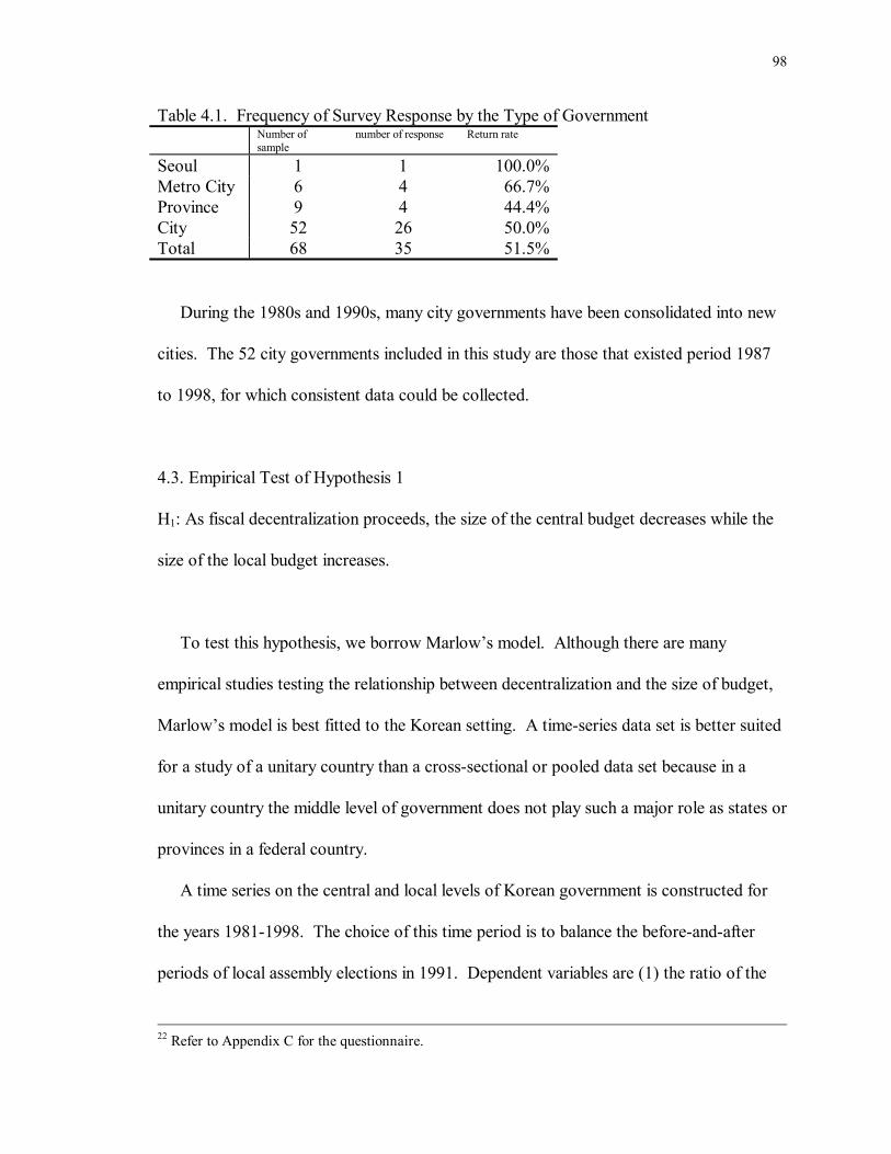
98

Table 4.1. Frequency of Survey Response by the Type of Government Number of

sample number of response Return rate

Seoul 1 1 100.0%Metro City 6 4 66.7%Province 9 4 44.4%City 52 26 50.0%Total 68 35 51.5%

During the 1980s and 1990s, many city governments have been consolidated into new

cities. The 52 city governments included in this study are those that existed period 1987

to 1998, for which consistent data could be collected.

4.3. Empirical Test of Hypothesis 1



To test this hypothesis, we borrow Marlow�s model. Although there are many

empirical studies testing the relationship between decentralization and the size of budget,

Marlow�s model is best fitted to the Korean setting. A time-series data set is better suited

for a study of a unitary country than a cross-sectional or pooled data set because in a

unitary country the middle level of government does not play such a major role as states or

provinces in a federal country.

A time series on the central and local levels of Korean government is constructed for

the years 1981-1998. The choice of this time period is to balance the before-and-after

periods of local assembly elections in 1991. Dependent variables are (1) the ratio of the

22 Refer to Appendix C for the questionnaire.

99

central government expenditure-to-GDP (CE), (2) the ratio of local government

expenditure-to-GDP (LE), and (3) the ratio of total government expenditure-to-GDP

(TE). A key independent variable is fiscal decentralization measured by the ratio of local

expenditure-to-total government expenditure (DEC).23 Control variables include real per

capita disposable income (INCOME)24 and population (POP). The income variable

controls the influence of Wagner�s Law that suggests a positive relationship between

government size and real income. The control for population acts as a scale variable.

Table 4.2. Operationalization of Variables (Hypothesis 1) Variables Operationalized Definition

CE Central government expenditure ÷ GDP

LE Local government expenditure ÷ GDP

TE Total government expenditure25 ÷ GDP

DEC (local government expenditure � conditional grants) ÷ (total government

expenditure � unconditional grants)

INCOME Per capita disposable income in 1995 constant won

POP Population

I conduct OLS regression analysis of three dependent variables (CE, LE, and TE) and

independent variable (DEC) (Table 4.3). The logistic transformation26 of dependent

23 Conditional grants such as national subsidies are excluded from the local expenditure and unconditional grants such as local shared tax are included as the local expenditure. Appendix D reports the regression estimation results without controlling those effects. 24 We use constant won (1995) instead of current won. Constant won = (current won/CPI)*100 25 central expenditure + local expenditure

100

variables is conducted because dependent variables have a range limited to the zero-to-one

interval, which is not satisfied with the basic assumption of the regression model.

Table 4.3. OLS Estimation of CE, LE, and TE (N=18) CE LE TE Intercept -0.681 -1.811 -0.723 (-5.945)*** (-18.222)*** (-5.761)*** DEC 7.48E-03 2.374 0.804 (0.019) (6.790)*** (0.821) R2 0.062 0.726 0.120 t-statistics in parentheses ** significant at the 5% level, two-tailed test; *** 1% The signs of DEC in all three equations are positive. This means a more decentralized

government tends to be associated with a larger amount of government spending.

We conduct OLS regression analysis with control variables (INCOME and POP)

(Table 4.4). In the CE equation and the TE equation, the sign of DEC is negative. This

means a more decentralized public sector is associated with less central spending and less

government total spending. In the LE equation, the sign of DEC is positive. This means a

more decentralized public sector is associated with more local spending, but there is no

statistically significant relationship between LE and DEC.

26 CE� = log CE

CE

−1

101

Table 4.4. OLS Estimation of CE, LE, AND TE with Control Variables (N=18) CE LE TE Intercept -0.421 -1.847 -0.461 (-0.390) (-2.025)* (-0.392) DEC -2.172 0.421 -1.597 (-3.667)*** (0.841) (-2.479)** INCOME 1.033E-06 7.449E-07 1.122E-06 (1.446) (1.235) (1.443) POP 3.029E-09 9.947E-09 3.991E-09 (0.103) (0.400) (0.125) D-W 0.628 0.643 0.625 Adjusted R2 0.479 0.873 0.574 t-statistics in parentheses * significant at the 10% level, two-tailed test; ** 5%; *** 1%

The Durbin-Watson d Test is used to detect an autocorrelation problem. The

computed d value must lie between 0 and 4. If a computed d value is closer to zero, there

is evidence of positive autocorrelation, and if it is closer to 4, there is evidence of negative

autocorrelation. The closer the d value is to 2, the more the evidence is in favor of no

autocorrelation.

We find all three equations suffer from autocorrelation. The GLS regression method27

is conducted as a remedial procedure. The usual procedure of GLS using generalized

difference equation is as follows.28

CEt = α0 + α1 DECt + α2 INCOMEt + α3 POPt + µt (equation 4.1)

102

and assume that the error terms follow the AR(1) scheme:

µt = ρµt-1 + νt 1 ≥ ρ ≥ -1 (equation 4.2)

where the νs satisfy the usual OLS assumption and ρ is known.

Now, if we can transform the model (equation 4.1) so that in the transformed model

the error term is serially independent, then applying OLS to the transformed model will

give us the usual BLUE estimators, assuming that other assumptions of CLRM are

fulfilled.

We can write the regression (equation 4.1) with a one-period lag as

CEt-1 = α0 + α1 DEC t-1 + α2 INCOME t-1 + α3 POP t-1 + µ t-1 (equation 4.3)

Multiply the regression (equation 4.3) by ρ on both sides to obtain

ρCEt-1 = ρα0 + ρα1 DEC t-1 + ρα2 INCOME t-1 + ρα3 POP t-1 + ρµ t-1 (equation 4.4)

Subtract equation 4.4 from equation 4.1, to yield

(CE t - ρCE t-1) = α0 (1 - ρ) + α1 (DEC t - ρDEC t-1) + α2 (INCOME t - ρINCOME t-1) +

α3 (POP t - ρPOP t-1) + µ t - ρµ t-1 (equation 4.5)

From equation 4.2, µ t - ρµ t-1 = νt

Therefore,

(CE t - ρCE t-1) = α0 (1 - ρ) + α1 (DEC t - ρDEC t-1) + α2 (INCOME t - ρINCOME t-1) +

α3 (POP t - ρPOP t-1) + νt (equation 4.6)

27 In simplest definition, GLS is OLS on the transformed variables that satisfy the standard least-squares assumptions (Gujarati 1995:363).

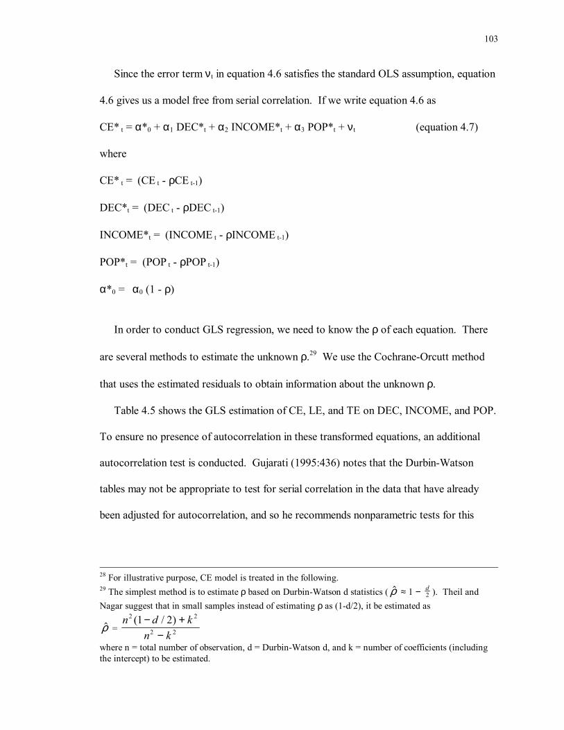
103

Since the error term νt in equation 4.6 satisfies the standard OLS assumption, equation

4.6 gives us a model free from serial correlation. If we write equation 4.6 as

CE* t = α*0 + α1 DEC*t + α2 INCOME*t + α3 POP*t + νt (equation 4.7)

where

CE* t = (CE t - ρCE t-1)

DEC*t = (DEC t - ρDEC t-1)

INCOME*t = (INCOME t - ρINCOME t-1)

POP*t = (POP t - ρPOP t-1)

α*0 = α0 (1 - ρ)

In order to conduct GLS regression, we need to know the ρ of each equation. There

are several methods to estimate the unknown ρ.29 We use the Cochrane-Orcutt method

that uses the estimated residuals to obtain information about the unknown ρ.

Table 4.5 shows the GLS estimation of CE, LE, and TE on DEC, INCOME, and POP.

To ensure no presence of autocorrelation in these transformed equations, an additional

autocorrelation test is conducted. Gujarati (1995:436) notes that the Durbin-Watson

tables may not be appropriate to test for serial correlation in the data that have already

been adjusted for autocorrelation, and so he recommends nonparametric tests for this

28 For illustrative purpose, CE model is treated in the following. 29 The simplest method is to estimate ρ based on Durbin-Watson d statistics ( $ρ ≈ 1 − d

2 ). Theil and Nagar suggest that in small samples instead of estimating ρ as (1-d/2), it be estimated as

$ρ = n d k

n k

2 2

2 2

1 2( / )− +−

where n = total number of observation, d = Durbin-Watson d, and k = number of coefficients (including the intercept) to be estimated.

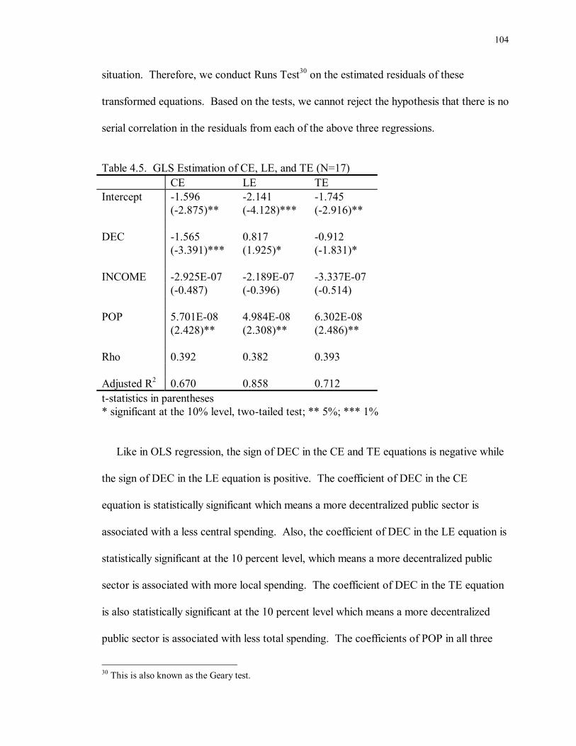
104

situation. Therefore, we conduct Runs Test30 on the estimated residuals of these

transformed equations. Based on the tests, we cannot reject the hypothesis that there is no

serial correlation in the residuals from each of the above three regressions.

Table 4.5. GLS Estimation of CE, LE, and TE (N=17) CE LE TE Intercept -1.596 -2.141 -1.745 (-2.875)** (-4.128)*** (-2.916)** DEC -1.565 0.817 -0.912 (-3.391)*** (1.925)* (-1.831)* INCOME -2.925E-07 -2.189E-07 -3.337E-07 (-0.487) (-0.396) (-0.514) POP 5.701E-08 4.984E-08 6.302E-08 (2.428)** (2.308)** (2.486)** Rho 0.392 0.382 0.393 Adjusted R2 0.670 0.858 0.712 t-statistics in parentheses * significant at the 10% level, two-tailed test; ** 5%; *** 1%

Like in OLS regression, the sign of DEC in the CE and TE equations is negative while

the sign of DEC in the LE equation is positive. The coefficient of DEC in the CE

equation is statistically significant which means a more decentralized public sector is

associated with a less central spending. Also, the coefficient of DEC in the LE equation is

statistically significant at the 10 percent level, which means a more decentralized public

sector is associated with more local spending. The coefficient of DEC in the TE equation

is also statistically significant at the 10 percent level which means a more decentralized

public sector is associated with less total spending. The coefficients of POP in all three

30 This is also known as the Geary test.

105

equations are statistically significant which means an increase in population is associated

with more public spending. Finally, the coefficients of INCOME in all three equations are

not statistically significant. This finding indicates that level of income does not affect the

level of public spending in Korea. As Bahl (1999) points out, this result may come from

the fact that voter preferences have not been revealed into either national or local budget

outcomes.

There may be a simultaneous relationship between two dependent variables (CE and

LE) and DEC because an increase in the central expenditure will increase total

government expenditure, leading to a decrease in the decentralization ratio. Or, an

increase in the local expenditure may lead to an increase in the decentralization ratio.

A basic assumption in a single equation regression model is that the Xs are the

exogenous variables. In other words, the causality, if any, runs from Xs to Y, not from Y

to Xs. However, there are situations in which such a unidirectional relationship between

Y and Xs cannot be maintained. It is quite possible that the Xs not only affect Y but Y

can also affect one or more Xs. If this is the case, the single equation modeling strategy

will not suffice.

A version of the Hausman specification error test is used for testing the simultaneity

problem in CE and LE equations.31

CEt = α0 + α1DECt + α2INCOMEt + α3POPt + µ1t (equation 4.8)

DECt = β0 + β1CEt + β2Xt + µ2t (equation 4.9)

X = a set of explanatory variables

31 For illustrative purpose, only CE equation is treated in the following.

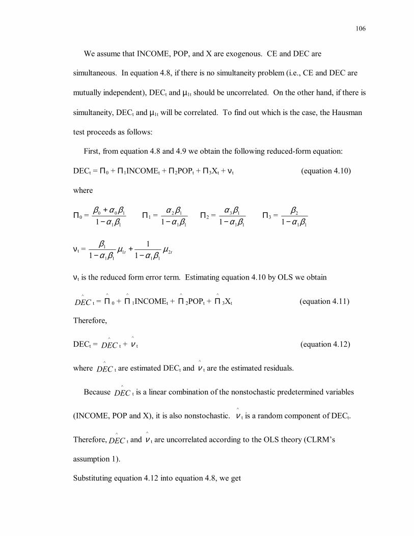
106

We assume that INCOME, POP, and X are exogenous. CE and DEC are

simultaneous. In equation 4.8, if there is no simultaneity problem (i.e., CE and DEC are

mutually independent), DECt and µ1t should be uncorrelated. On the other hand, if there is

simultaneity, DECt and µ1t will be correlated. To find out which is the case, the Hausman

test proceeds as follows:

First, from equation 4.8 and 4.9 we obtain the following reduced-form equation:

DECt = Π0 + Π1INCOMEt + Π2POPt + Π3Xt + νt (equation 4.10)

where

Π0 = 11

100

1 βαβαβ

−+

Π1 = 11

12

1 βαβα

− Π2 =

11

13

1 βαβα

− Π3 =

11

2

1 βαβ

−

νt = tt 211

111

1

11

1µ

βαµ

βαβ

−+

−

νt is the reduced form error term. Estimating equation 4.10 by OLS we obtain

DEC^

t = Π^

0 + Π^

1INCOMEt + Π^

2POPt + Π^

3Xt (equation 4.11)

Therefore,

DECt = DEC^

t + ν^

t (equation 4.12)

where DEC^

t are estimated DECt and ν^

t are the estimated residuals.

Because DEC^

t is a linear combination of the nonstochastic predetermined variables

(INCOME, POP and X), it is also nonstochastic. ν^

t is a random component of DECt.

Therefore, DEC^

t and ν^

t are uncorrelated according to the OLS theory (CLRM�s

assumption 1).

Substituting equation 4.12 into equation 4.8, we get

107

CEt = α0 + α1 DEC^

t + α2INCOMEt + α3POPt + α1ν^

t + µ1t (equation 4.13)

In order to know whether DECt and µ1t are correlated, we test the relationship between

ν^

t and µ1t in equation 4.13 because DEC^

t is nonstochastic and ν^

t is the random

component of DECt.

Now under the null hypothesis that there is no simultaneity, the correlation between ν^

t

and µ1t should be zero, asymptotically, that is, as the sample size increases indefinitely.

Thus, if we run the regression and find that the coefficient of ν^

t in equation 4.13 is

statistically zero, we can conclude that there is no simultaneity problem. This conclusion

will be reversed if we find this coefficient to be statistically significant.

We find a simultaneity problem only in the CE equation. So, there is a need for a

remedial procedure for the CE equation. The two-stage least squares (2SLS) method is

used as a remedial method. The usual procedure of 2SLS method is as follows:

CEt = α0 + α1DECt + α2INCOMEt + α3POPt + µ1t (equation 4.8)

DECt = β0 + β1CEt + β2Xt + µ2t (equation 4.9)

! Stage 1.

To get rid of the likely correlation between DEC and µ1, regress first DEC on all the

predetermined variables. Therefore,

DECt = Π^

0 + Π^

1INCOMEt + Π^

2POPt + Π^

3Xt + µ^

t (equation 4.14)

where µ^

t are the usual OLS residuals. From equation 4.14 we obtain

108

DEC^

t = Π^

0 + Π^

1INCOMEt + Π^

2POPt + Π^

3Xt (equation 4.15)

Equation 4.14 can be expressed as

DECt = DEC^

t + µ^

t (equation 4.16)

which shows that the stochastic DEC consists of two parts: DEC^

t, which is a linear

combination of the nonstochastic predetermined variables (INCOME, POP and X), and a

random component µ^

t. Following the OLS theory (CLRM�s assumption 1), DEC^

t and

µ^

t are uncorrelated.

! Stage 2.

Equation 4.8 can be written as

CEt = α0 + α1( DEC^

t + µ^

t) + α2INCOMEt + α3POPt + µ1t

= α0 + α1 DEC^

t + α2INCOMEt + α3POPt + (µ1t + α1 µ^

t)

= α0 + α1 DEC^

t + α2INCOMEt + α3POPt + µ*t (equation 4.17)

where µ*t = µ1t + α1 µ

^

t

Although DEC in equation 4.8 is correlated or likely to be correlated with the

disturbance term µ1 (hence rendering OLS inappropriate), DEC^

t in equation 4.17 is

uncorrelated with µ*t asymptotically because the error term, µ*

t, contains µ^

t, which is an

uncorelated error term with DEC^

t. As a result, OLS can be applied to equation 4.17.

109

Also, there is another important procedure to conduct 2SLS. In order to conduct OLS

estimation of equation 4.17, we should have DEC^

t, not DECt. In order to get DEC^

t, we

use instrumental variables, which are highly correlated with DECt but are uncorrelated

with µ*t.

Table 4.6. 2SLS Estimation of CE (N = 18) CE Intercept -0.367 (-0.337) DEC -1.946 (-2.466)** INCOME 1.009E-06 (1.403) POP 4.144E-10 (0.014) Adjusted R2 0.32 t-statistics in parentheses ** significant at 5% level, two-tailed test

Table 4.6 shows the result of 2SLS regression.32 DEC still has a negative coefficient of

statistical significance, which means a more decentralized government tends to be

associated with a less central spending.

During the last 20 years, defense spending in relation to GDP has declined (Figure 4.1).

Because defense expenditures have occupied a big portion of central government

expenditures, its decrease affects the level of central spending. Therefore, the conclusion

32 Instruments employed are the exogenous variables in the model and the ratio of import and export to GDP. The import/export ratio is correlated to DEC (-0.623) but it is not correlated to CE (0.113).

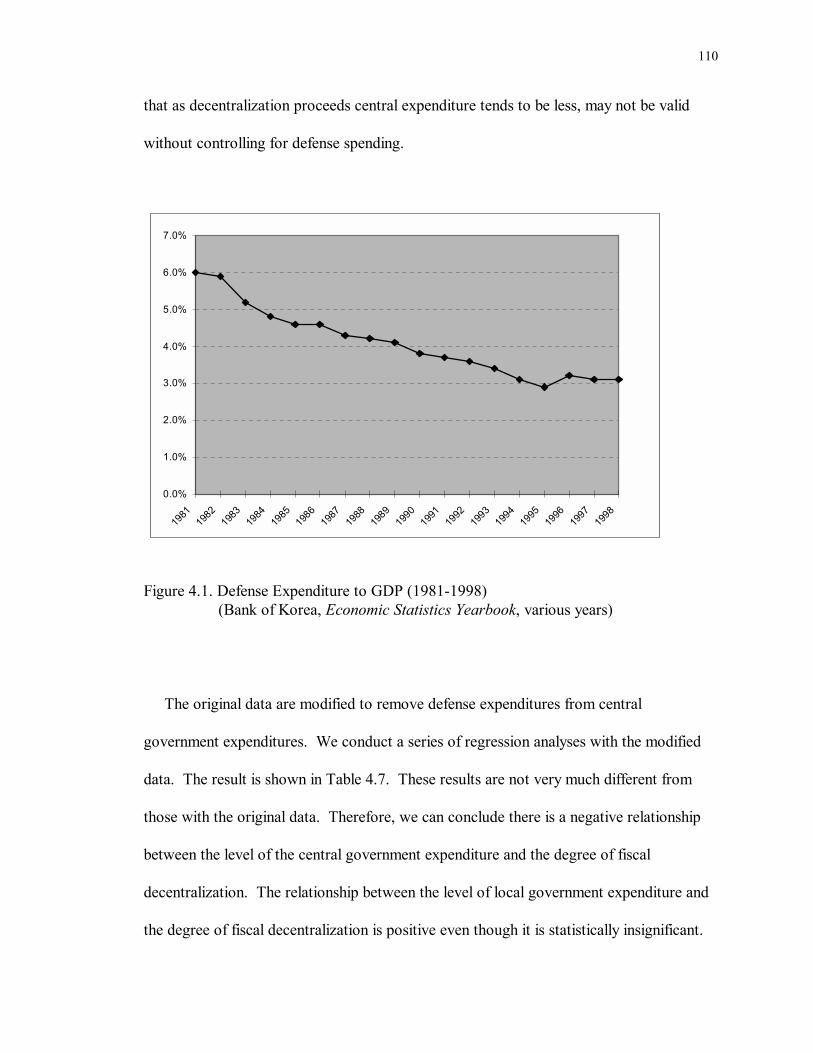
110

that as decentralization proceeds central expenditure tends to be less, may not be valid

without controlling for defense spending.

Defense/GDP Expenditure*1981 6.0% 2853.71982 5.9% 3185.21983 5.2% 3343.61984 4.8% 3539.91985 4.6% 3750.21986 4.6% 4335.51987 4.3% 4793.51988 4.2% 5572.11989 4.1% 6147.41990 3.8% 6854.01991 3.7% 8012.01992 3.6% 8770.81993 3.4% 9308.11994 3.1% 10055.51995 2.9% 11050.61996 3.2% 13216.71997 3.1% 14161.21998 3.1% 13964.3

0.0%

1.0%

2.0%

3.0%

4.0%

5.0%

6.0%

7.0%

1981

1982

1983

1984

1985

1986

1987

1988

1989

1990

1991

1992

1993

1994

1995

1996

1997

1998

Figure 4.1. Defense Expenditure to GDP (1981-1998) (Bank of Korea, Economic Statistics Yearbook, various years)

The original data are modified to remove defense expenditures from central

government expenditures. We conduct a series of regression analyses with the modified

data. The result is shown in Table 4.7. These results are not very much different from

those with the original data. Therefore, we can conclude there is a negative relationship

between the level of the central government expenditure and the degree of fiscal

decentralization. The relationship between the level of local government expenditure and

the degree of fiscal decentralization is positive even though it is statistically insignificant.

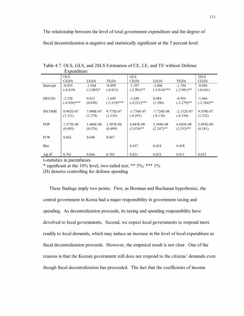
111

The relationship between the level of total government expenditure and the degree of

fiscal decentralization is negative and statistically significant at the 5 percent level.

Table 4.7. OLS, GLS, and 2SLS Estimation of CE, LE, and TE without Defense Expenditure OLS GLS 2SLS CE(D) LE(D) TE(D) CE(D) LE(D) TE(D) CE(D) Intercept -0.835 -1.944 -0.899 -1.587 -2.006 -1.744 -0.696 (-0.819) (-2.085)* (-0.813) (-2.901)** (-3.814)*** (-2.981)** (-0.641) DEC(D) -2.258 0.012 -1.649 -1.649 0.484 -0.954 -1.666 (-4.926)*** (0.030) (-3.319)*** (-4.221)*** (1.296) (-2.279)** (-2.364)** INCOME 8.992E-07 7.890E-07 9.775E-07 -1.734E-07 -7.724E-08 -2.132E-07 9.539E-07 (1.331) (1.278) (1.335) (-0.291) (-0.136) (-0.334) (1.332) POP 1.373E-08 1.466E-08 1.507E-08 6.043E-08 5.248E-08 6.682E-08 5.493E-09 (0.493) (0.576) (0.499) (2.474)** (2.247)** (2.553)** (0.181) D-W 0.662 0.648 0.667 Rho 0.437 0.434 0.438 Adj R2 0.761 0.866 0.783 0.821 0.822 0.811 0.652 t-statistics in parentheses * significant at the 10% level, two-tailed test; ** 5%; *** 1% (D) denotes controlling for defense spending

These findings imply two points. First, as Brennan and Buchanan hypothesize, the

central government in Korea had a major responsibility in government taxing and

spending. As decentralization proceeds, its taxing and spending responsibility have

devolved to local governments. Second, we expect local governments to respond more

readily to local demands, which may induce an increase in the level of local expenditure as

fiscal decentralization proceeds. However, the empirical result is not clear. One of the

reasons is that the Korean government still does not respond to the citizens� demands even

though fiscal decentralization has proceeded. The fact that the coefficients of income

112

variables in all equations do not have statistical significance may also provide a partial

indication that the Korean government does not readily respond to the citizens� demands.



expenditure increase.

A time series on 59 city governments is constructed for the years 1987-1998. This part

of the study uses a panel data set. Hsiao (1986) argues the advantages of panel data sets

over conventional cross-sectional or time-series data sets are as follows. First, because

panel data sets usually have a large number of data points, they increase the degrees of

freedom and reduce the collinearity among explanatory variables. Second, panel data sets

contrast cross-sections of a unit on one dimension as well as points of time for each unit

on another. By pooling these two dimensions, they combine the virtues and few of the

limitations of cross-sectional or time-series analysis. Although panel data sets have several

virtues mentioned above, they are not immune from econometric problems such as

heteroscedasticity and autocorrelation.

The dependent variables are the levels of redistribution and economic development

expenditures. To reclassify local expenditure into those two functional areas is subject to

imprecision and subjectivity. For the purpose of this study, however, reclassification is

necessary. The functional classification of local expenditures reported in the Financial

Yearbook of Local Government is rearranged. Social Welfare expenditure is classified as

113

redistribution expenditure. Industry and Economy, and Regional Development are

classified as developmental expenditure.


RED Per capita redistribution expenditure in 1995 constant won

DEV Per capita developmental expenditure in 1995 constant won

DEC Own-source revenue ÷ total revenue

LAG(RED) One-time-period lagged value of RED

LAG(DEV) One-time-period lagged value of DEV

INCOME Per capita gross regional product (GRP)

DENSITY Number of residents per km2

GRANT Per capita grants in 1995 constant won

CITY Dummy variable. D=1 if Seoul or metropolitan cities. D=0 otherwise

POP Population

The independent variable is the self-reliance rate of local government.33 Because this

part of the study is concerned with local expenditures only, the expenditure

decentralization figure, which was the share of local expenditures to total expenditures in

the previous model, cannot be obtained. Therefore, the alternative measure of

decentralization employed is the self-reliance rate of local governments.

33 The self-reliance rate of a jurisdiction is calculated as own-source revenue divided by total revenue.

114

Dependent variables34 are measured as (1) per capita redistribution expenditure (RED)

and (2) per capita developmental expenditure (DEV). A key independent variable is fiscal

decentralization measured by the self-reliance rate of each local jurisdiction (DEC).

As mentioned earlier, we identify several important determinants of local expenditure:

(1) incrementalism, (2) fiscal capacity, (3) demand for service, (4) cost of supplying

services, and (5) intergovernmental grants. To capture those determinants into our model,

we use some additional variables. First, we use a one-time-period lagged (t-1) ratio of

each functional expenditure (LAG(RED) and LAG(DEV)) to capture incrementalism.

Second, fiscal capacity of a local government is measured by Gross Regional Product

(GRP) per capita (INCOME).35 Ladd and Yinger (1989) ague that fiscal capacity of local

governments can be measure by the resident�s income. If a local jurisdiction has a broad

tax base and strong economic activities, its resident�s income is different from other

jurisdictions, which have weak economic activities. Third, demand for services and cost

of supplying services are measured by number of residents per km2 (DENSITY). Because

population density is usually correlated with wage rates and the price of many materials, it

may be accepted as a proxy for variations in the demand for and the cost of government

services (Peterson 1981:52). Fourth, intergovernmental grants are measured by per-capita

grant (GRANT).36 Intergovernmental grants tend to stimulate spending by the

government that receives the grants (Oates, 1985; Grossman, 1989). Therefore, it is one

34 We use 1995 constant won. 35 Because Korean government has not published any income data by city, this study uses Lee and Kim�s (1990:107) method to estimate GRP. This method also appears in Ahn�s dissertation (American University 1995). GRP is calculated as the total amount of tax burden (national + local tax amount) divided by tax burden rate. This method assumes that income change is in proportion to tax burden change. Another common practice to incorporate income data into a model in the Korean literature is to use the number of cars. 36 We use constant won for per-capita grant.

115

factor determining the size of the local budget. Finally, we use city dummy (CITY)37 and

population (POP) as scale variables.

We conduct OLS regression estimation of two equations. The models estimated are

REDit = α0 + α1 DECit + α2 LAG(RED)it + α3 INCOMEit + α4 DENSITYit +

α5 GRANTit + α6 CITYit + α7 POPit + µit (equation 4.18)

DEVit = β0 + β1 DECit + β2 LAG(DEV)it + β3 INCOMEit + β4 DENSITYit +

β5 GRANTit + β6 CITYit + β7 POPit + νit (equation 4.19)

The estimation result is shown in Table 4.9. At this point, a single most important

finding is that the levels of redistributive and developmental expenditures are positively

associated with the degree of fiscal decentralization.

However, given that the data set consists of cross-sections of cities, it will presumably

have a typical heteroscedasticity problem. In Figure 4.2 and 4.3, squared residuals from

OLS estimations of RED and DEV equations are plotted against the predicted values of

dependent variables. We cannot conclude whether the pattern of the relationship is

random or not.

37 D = 1, if city is Seoul or metropolitan city; D = 0, otherwise

116

Table. 4.9. OLS Estimation of RED and DEV (N = 708) RED DEV Intercept -12196.57 -36672.01 (-2.704)*** (-3.664)*** DEC 17435.789 102777.41 (2.383)** (6.261)*** LAG(RED) 0.923 (37.638)*** LAG(DEV) 0.387 (13.203)*** INCOME 1.20E-03 5.437E-03 (4.227)*** (8.696)*** DENSITY 0.367 -2.958 (0.853) (-3.158)*** GRANT 6.381E-02 0.377 (9.804)*** (20.341)*** CITY -2611.113 -3026.369 (-0.713) (-0.385) POP -1.170E-03 1.640E-03 (-1.176) (0.765) Adjusted R2 0.882 0.887 t-statistics in parentheses * significant at the 10% level, two-tailed test; ** 5%; *** 1%

117

Predicted value of welfare expenditure

4000003000002000001000000

Squa

red

OLS

resi

dual

s

20000000000

10000000000

100

Figure 4.2. Structure of the Heteroscedasticity (RED)

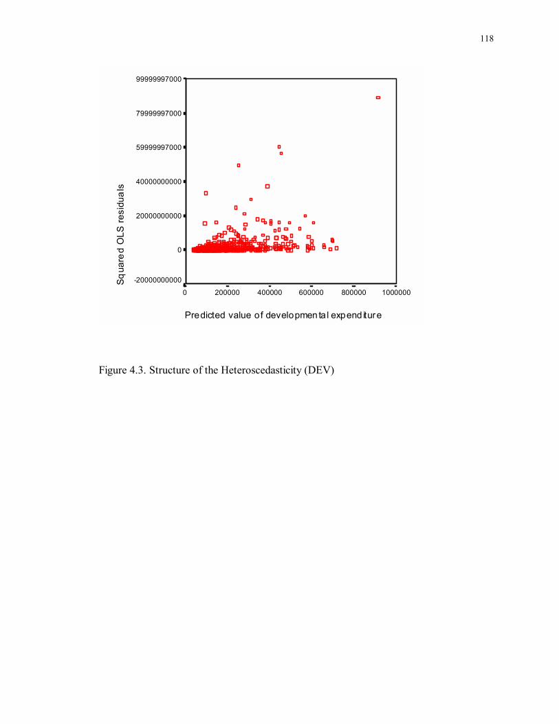
118

Predicted value of developmental expend iture

10000008000006000004000002000000

Squa

red

OLS

resi

dual

s

99999997000

79999997000

59999997000

40000000000

20000000000

0

-20000000000

Figure 4.3. Structure of the Heteroscedasticity (DEV)

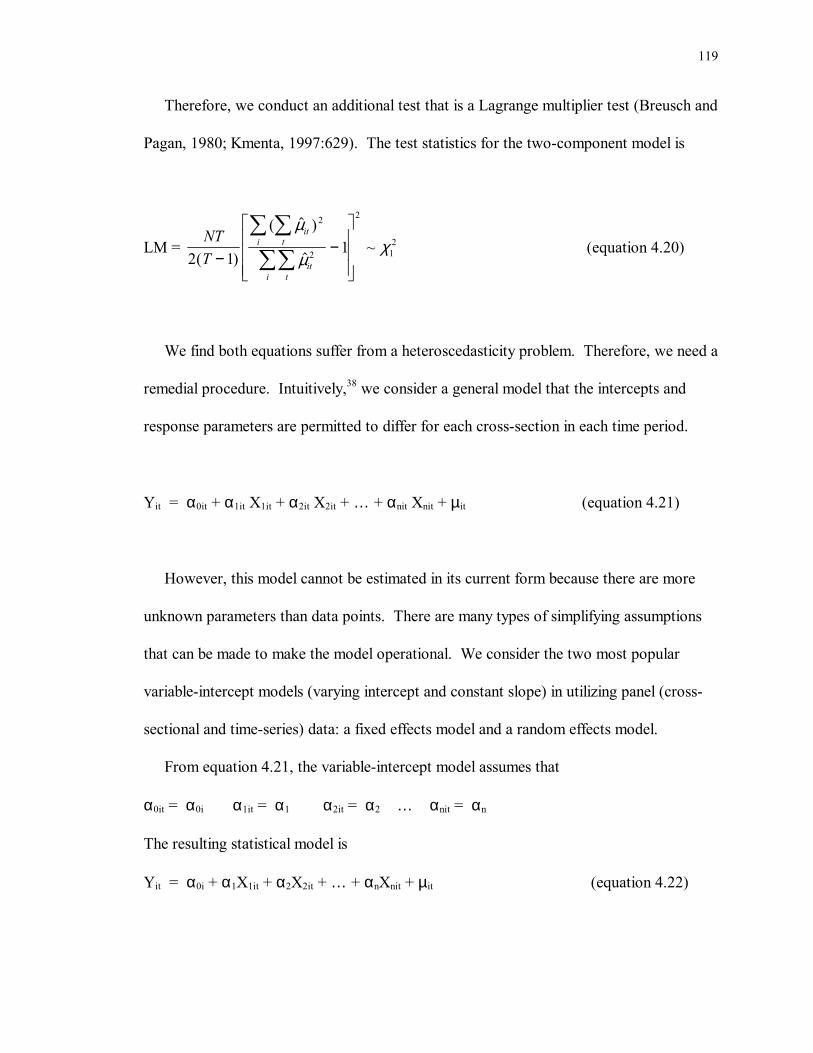
119

Therefore, we conduct an additional test that is a Lagrange multiplier test (Breusch and

Pagan, 1980; Kmenta, 1997:629). The test statistics for the two-component model is

LM = NTT

itti

itti

2 11

2

2

2

12

( )

( $ )

$~

−−

∑∑∑∑

µ

µχ (equation 4.20)

We find both equations suffer from a heteroscedasticity problem. Therefore, we need a

remedial procedure. Intuitively,38 we consider a general model that the intercepts and

response parameters are permitted to differ for each cross-section in each time period.

Yit = α0it + α1it X1it + α2it X2it + … + αnit Xnit + µit (equation 4.21)

However, this model cannot be estimated in its current form because there are more

unknown parameters than data points. There are many types of simplifying assumptions

that can be made to make the model operational. We consider the two most popular

variable-intercept models (varying intercept and constant slope) in utilizing panel (cross-

sectional and time-series) data: a fixed effects model and a random effects model.

From equation 4.21, the variable-intercept model assumes that

α0it = α0i α1it = α1 α2it = α2 … αnit = αn

The resulting statistical model is

Yit = α0i + α1X1it + α2X2it + … + αnXnit + µit (equation 4.22)

120

In equation 4.22, the intercepts vary but the slopes are constant for cross-sections in

time periods. The feature that distinguishes the fixed effects model from the random

effects model is the way in which the varying intercept, α0i, is treated. As the name

implies, the fixed effects model treats it as a fixed, unknown parameter while the random

effects model treats it as random drawings from the population distribution of cross-

section intercepts. The following section shows how each approach estimates equation

4.22.

The fixed effects model introduces a set of dummy variables to estimate equation 4.22.

This method is known as LSDV (least squares dummy variable). The dummy variables

are defined as follows.

D1i = 1, i = 1 D2i = 1, i = 2 D3i = 1, i = 3 … DNi = 1, i = N 0, otherwise 0, otherwise 0, otherwise 0, otherwise

Under these definitions equation 4.22 becomes

Yit = α01D1i + α02D2i + α03D3i + … + α0NDNi +

α1X1it + α2X2it + … + αnXnit + µit (equation 4.23)

In equation 4.23 there are N dummy variables, one for each cross-section. Therefore,

each cross-sectional unit has its own intercept value, but it stays constant over time within

each cross-sectional unit. The differences between cross-sectional units are reflected in

the coefficients, α0N.

38 This intuition comes from the fact that the previous OLS model presumes the intercept and response parameter remain the same for all the cross-sections and time periods.

121

This is a reasonable approach when the differences between cross-sectional units can

be viewed as parametric shifts of the regression function. However, its estimation result is

strictly conditioned on the sample in the study, and we cannot apply the result to outside-

the-sample cross-sections. Also, because it introduces additional N dummy variables into

the model, it loses N number of degrees of freedom. This is an important issue when the

sample size is relatively small.

Another disadvantage of using LSDV is that its estimation result is biased when the

model has a particular type of explanatory variable. LSDV is unable to provide the

coefficient of a variable that remains unchanged over time within each cross-sectional unit

(e.g., dummy variable). When a model has a lagged dependent variable as an explanatory

variable, the estimation result of LSDV tends to be underestimated (Hsiao, 1986:95).

In the random effects model, we assume the intercepts (α0i in equation 4.22) are

random variables. Therefore, the intercepts (α0i) are modeled as39

α0i = α 0 + εi i = 1, �., N (equation 4.24)

α 0 is an unknown parameter that represents the population mean intercept, and εi is an

unobservable random error that accounts for individual differences in cross-sectional

behavior. We assume that the εi are independent of each other and µit in equation 4.22.

Substituting equation 4.24 into 4.22 yields

39 In this case we consider two components model. Although most econometrics textbooks deal with three components model (νit = εi + λt + µit) in theoretical basis, most applied studies omit the time component and use two components model (Kmenta 1997:627). Stimson (1985:926) argues that this practice comes

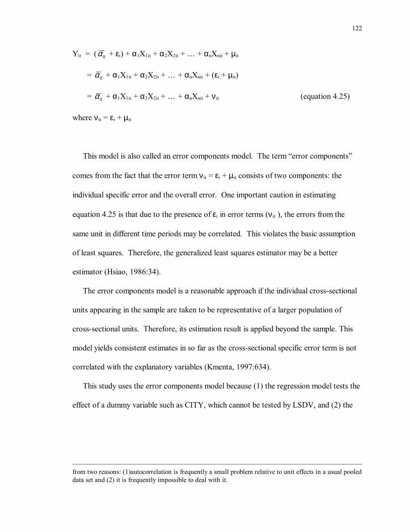
122

Yit = (α 0 + εi) + α1X1it + α2X2it + … + αnXnit + µit

= α 0 + α1X1it + α2X2it + … + αnXnit + (εi + µit)

= α 0 + α1X1it + α2X2it + … + αnXnit + νit (equation 4.25)

where νit = εi + µit

This model is also called an error components model. The term �error components�

comes from the fact that the error term νit = εi + µit consists of two components: the

individual specific error and the overall error. One important caution in estimating

equation 4.25 is that due to the presence of εi in error terms (νit ), the errors from the

same unit in different time periods may be correlated. This violates the basic assumption

of least squares. Therefore, the generalized least squares estimator may be a better

estimator (Hsiao, 1986:34).

The error components model is a reasonable approach if the individual cross-sectional

units appearing in the sample are taken to be representative of a larger population of

cross-sectional units. Therefore, its estimation result is applied beyond the sample. This

model yields consistent estimates in so far as the cross-sectional specific error term is not

correlated with the explanatory variables (Kmenta, 1997:634).

This study uses the error components model because (1) the regression model tests the

effect of a dummy variable such as CITY, which cannot be tested by LSDV, and (2) the

from two reasons: (1)autocorrelation is frequently a small problem relative to unit effects in a usual pooled data set and (2) it is frequently impossible to deal with it.

123

model includes a lagged dependent variable as an explanatory variable that may cause a

biased estimation by LSDV.40

In order to conduct GLS estimation of the error components model, we need to know

ρ (ρ = σu2/σ2). There are several methods to estimate the unknown ρ. Stimson

(1985:924-925) argues that �estimator efficiency41 is relatively insensitive to the quality of

variance component estimates.� We use a two-step GLS estimation (Stimson, 1985:937).

The usual procedure is as follows.

σ2 = σu2 + σe

2 (equation 4.26)

where σ2 is the total residual variance, σu2 is the between-group residual variance, and σe

2

is the within-group residual variance.

The total variance σ2 may be estimated from the residual variance of the OLS estimation.

The within-group variance σe2 may be estimated from the residual variance of the LSDV

estimation. Then, the estimate of ρ is the ratio σu2/σ2.

Table 4.10 shows GLS estimation of the error-components model (GLSE). The key

independent variable, the degree of decentralization, is positively associated with the levels

of redistributive expenditure and developmental expenditure. This finding suggests that as

fiscal decentralization proceeds, local governments increase the levels of redistributive and

developmental expenditures.

The coefficients on LAGs are positive and statistically significant in both cases. This

indicates that the amount of budget in year t is strongly associated with the amount of

budget in year t-1. The coefficients on INCOMEs are positive and statistically significant

40 For dynamic model, GLS estimator in the error components model may be also biased. But its bias is smaller than that of OLS or LSDV (Hsiao, 1986:88). An alternative method will be maximum-likelihood

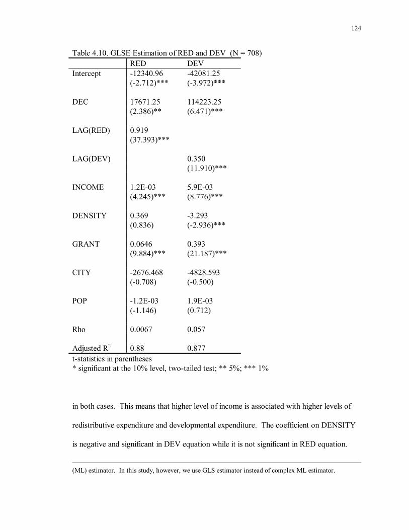
124

Table 4.10. GLSE Estimation of RED and DEV (N = 708) RED DEV Intercept -12340.96 -42081.25 (-2.712)*** (-3.972)*** DEC 17671.25 114223.25 (2.386)** (6.471)*** LAG(RED) 0.919 (37.393)*** LAG(DEV) 0.350 (11.910)*** INCOME 1.2E-03 5.9E-03 (4.245)*** (8.776)*** DENSITY 0.369 -3.293 (0.836) (-2.936)*** GRANT 0.0646 0.393 (9.884)*** (21.187)*** CITY -2676.468 -4828.593 (-0.708) (-0.500) POP -1.2E-03 1.9E-03 (-1.146) (0.712) Rho 0.0067 0.057 Adjusted R2 0.88 0.877 t-statistics in parentheses * significant at the 10% level, two-tailed test; ** 5%; *** 1%

in both cases. This means that higher level of income is associated with higher levels of

redistributive expenditure and developmental expenditure. The coefficient on DENSITY

is negative and significant in DEV equation while it is not significant in RED equation.

(ML) estimator. In this study, however, we use GLS estimator instead of complex ML estimator.

125

This finding indicates that a city with less population density is likely to spend more

developmental expenditure. The coefficients on GRANTs are positive and statistically

significant in both cases. This means that intergovernmental revenues support a certain

portion of redistributive and developmental expenditures.

In the survey, 24 out of 35 local governments respond that they put the most emphasis

on economic development. Eight out of 35 local governments respond that they put the

most emphasis on welfare function. From these survey results, we may notice that the two

most important policy areas in local governments are economic development and welfare

functions.


H3: As fiscal decentralization proceeds, fiscal independence of local governments

increases.

A data series on 59 city governments is constructed for the years 1987-1998. The

dependent variable is the self-reliance rate of each city government (SER). The self-

reliance rate is not a perfect measure of the fiscal independence of local governments in

that it neglects the expenditure side of local finance. It is, however, commonly used to

measure fiscal independence of local governments in Korean literature (Lim, 1997). Key

independent variables are qualitative measures of decentralization using a dummy variable

41 unbiased estimator with the least variance

126

(DDEC1 and DDEC2).42 The degree of decentralization is divided into two phases: local

assembly elections since 1991 and mayor elections since 1995.

Bahl and others (1994, 1986) argue that government structure is a critical element in

decentralization implementation especially in developing countries. Elected local

government is a necessary condition for decentralization. During the periods of 1991 and

1995, city government structure was one with locally elected assemblies and centrally

appointed mayors. Some question the quality of the local assembly in terms of its

expertise and experience. Because there had been no local assembly for several decades

and the Korean people were accustomed to an �executive-dominated� government system

as a result of military autocracy, the �new-born� local assembly was not expected to

perform its task well but just symbolized progress in democratic governance. Many

Koreans think real progress in local autonomy has started since the 1995 mayor elections.

There may be several other factors affecting the degree of the self-reliance rate of a

local government. First, fiscal capacity of a local government can affect the degree of the

self-reliance rate. If a local jurisdiction has a broad tax base and strong economic

activities, its self-reliance rate will increase. This is measured by an income proxy

(INCOME).43 Second, if a local government has more public programs in which the

benefits and costs are not retained within that jurisdiction, its self-reliance rate will

decrease because the central grants adjust those externalities. This is measured by the

local expenditure per capita devoted to roads, flood control, and other construction

42 Ddec1 = 1 1995 ≥ t ≥ 1992, Ddec1 = 0 otherwise; Ddec2 = 1 1998 ≥t ≥1996, Ddec2 = 0 otherwise. We introduce two dummy variables to depict the three periods (1987-1991, 1992-1995, and 1996-1998). Using only two dummy variables for three categories is a strategy to avoid dummy variable trap. 43 Gross Regional product (GRP) per capita

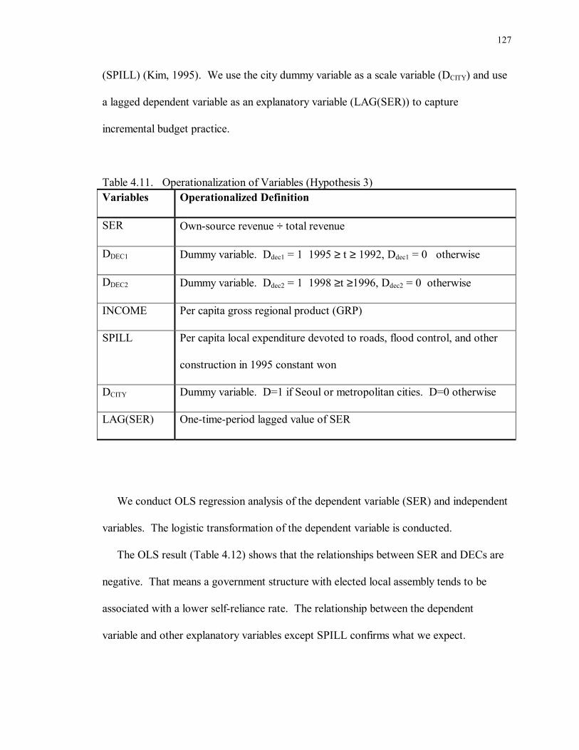
127

(SPILL) (Kim, 1995). We use the city dummy variable as a scale variable (DCITY) and use

a lagged dependent variable as an explanatory variable (LAG(SER)) to capture

incremental budget practice.


SER Own-source revenue ÷ total revenue

DDEC1 Dummy variable. Ddec1 = 1 1995 ≥ t ≥ 1992, Ddec1 = 0 otherwise

DDEC2 Dummy variable. Ddec2 = 1 1998 ≥t ≥1996, Ddec2 = 0 otherwise

INCOME Per capita gross regional product (GRP)

SPILL Per capita local expenditure devoted to roads, flood control, and other

construction in 1995 constant won

DCITY Dummy variable. D=1 if Seoul or metropolitan cities. D=0 otherwise

LAG(SER) One-time-period lagged value of SER

We conduct OLS regression analysis of the dependent variable (SER) and independent

variables. The logistic transformation of the dependent variable is conducted.

The OLS result (Table 4.12) shows that the relationships between SER and DECs are

negative. That means a government structure with elected local assembly tends to be

associated with a lower self-reliance rate. The relationship between the dependent

variable and other explanatory variables except SPILL confirms what we expect.

128

Table 4.12. OLS Estimation of SER (N = 708) SER Intercept -0.934 (-28.764)*** DDEC1 -9.072E-02 (-4.154)*** DDEC2 -6.139E-02 (-2.239)** INCOME 2.023E-08 (7.262)*** SPILL -0.216 (-1.916)* DCITY 8.979E-02 (3.357)*** LAG(SER) 1.990 (38.455)*** Adjusted R2 0.835 t-statistics in parentheses * significant at the 10% level, two-tailed test; ** 5%; *** 1%

However, given that the data set consists of cross-sections of cities, it will presumably

have a typical heteroscedasticity problem. Therefore, we use the error components model

for the same reasons mentioned in section 4.4. The model estimated is

SERit = α0i + α1DDEC1it + α2DDEC2it + α3INCOME1it + α4SPILLit + α5DCITYit +

α6LAG(SER)it + µit (equation 4.27)

DDEC1 = 1 if 1995 ≥ t ≥1992,

= 0 otherwise

129

DDEC2 = 1 if 1998 ≥ t ≥ 1996,

= 0 otherwise

i = 1,2��59

t = 1987, 1988 �..1998

Table 4.13. GLSE Estimation of SER (1987 � 1998) (N = 708) SER Intercept -0.731 (-17.196)*** DDEC1 -0.042 (-2.058)** DDEC2 -0.0319 (-1.230) INCOME 0.000a

(5.170)*** SPILL -0.233 (-2.143)** DCITY 0.095 (2.101)** LAG(SER) 1.649 (24.158)*** Rho 0.292 Adjusted R2 0.582 t-statistics in parentheses a denotes extremely small value * significant at the 10% level, two-tailed test; ** 5%; *** 1%

Table 4.13 reports GLS estimation of the error components model. DDEC1 is negatively

associated with the level of self-reliance rate. This means that the presence of local

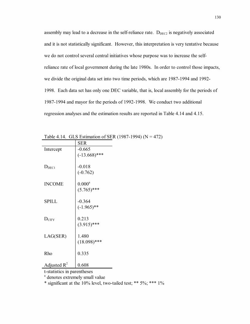
130

assembly may lead to a decrease in the self-reliance rate. DDEC2 is negatively associated

and it is not statistically significant. However, this interpretation is very tentative because

we do not control several central initiatives whose purpose was to increase the self-

reliance rate of local government during the late 1980s. In order to control those impacts,

we divide the original data set into two time periods, which are 1987-1994 and 1992-

1998. Each data set has only one DEC variable, that is, local assembly for the periods of

1987-1994 and mayor for the periods of 1992-1998. We conduct two additional

regression analyses and the estimation results are reported in Table 4.14 and 4.15.

Table 4.14. GLS Estimation of SER (1987-1994) (N = 472) SER Intercept -0.665 (-13.668)*** DDEC1 -0.018 (-0.762) INCOME 0.000a

(5.765)*** SPILL -0.364 (-1.965)** DCITY 0.213 (3.915)*** LAG(SER) 1.480 (18.098)*** Rho 0.335 Adjusted R2 0.608 t-statistics in parentheses a denotes extremely small value * significant at the 10% level, two-tailed test; ** 5%; *** 1%

131

Table 4.15. GLS Estimation of SER (1992-1998) (N = 413) SER Intercept -0.891 (-12.277)*** DDEC2 0.032 (1.699)* INCOME 0.000a

(2.215)** SPILL -0.240 (-1.916)* DCITY 0.096 (1.660)* LAG(SER) 1.874 (19.233)*** Rho 0.349 Adjusted R2 0.635 t-statistics in parentheses a denotes extremely small value * significant at the 10% level, two-tailed test; ** 5%; *** 1%

Comparing Table 4.13, 4.14, and 4.15, we can see the signs of the variables remain the

same except DDEC2. DDEC2 in Table 4.13 has negative sign and DDEC2 in Table 4.15 has

positive sign. The positive sign may mean that the introduction of an elected mayor may

lead to an increase in the self-reliance rate of local governments. In other words, the

elected mayors may contribute an increase in fiscal independence of local governments.

For the case of DDEC1, its coefficient is statistically significant in Table 4.13, but it is not

statistically significant in Table 4.14. This means the introduction of elected local

assembly may not be associated with the level of self-reliance rate.

132

This point is consistent with the survey results. Out of 35 responses, 33 local officials

say the office of mayor has more influence in determining the final budget outcome than

local assembly. Even though substantial percentages of local officials (23 out of 35)

respond that the local assembly plays an important role in determining the final budget

outcome, the role of the local assembly is somewhat limited because of its short history

and lack of expertise. Out of 35, only 3 local officials respond that local assemblymen are

well equipped with professional knowledge about budget substance. In the Korean

context, therefore, the introduction of an elected executive has more impact on fiscal

independence of local jurisdiction than the introduction of an elected assembly.

133

CHAPTER 5

SUMMARY AND CONCLUSION

The purpose of this study is to investigate the actual effects of decentralization on three

important aspects of public finance in Korea: public spending, functional responsibility,

and the fiscal independence of local government. Fiscal decentralization is considered to

have the potential to improve the performance of the public sector. Fiscal federalism

theory holds that the decentralized provision of public goods can increase efficiency in

resource allocation because local governments can be better tailored to the geographical

benefit areas of public goods, local governments are better positioned to recognize local

preferences and needs, and pressure from interjurisdictional competition may motivate

local governments to be innovative and accountable to their residents. The theory also

holds that redistribution and stabilization functions should be the central government�s

task because of the mobility of economic units.

However, some recent studies have challenged these conventional arguments on

theoretical and empirical grounds. Bahl and others (1994, 1986) hold that political, fiscal,

and administrative structures in developing countries are organized in such a way that

local voter preferences may not be readily revealed and incorporated into local budget

outcomes. As a result, the decentralized provision of public goods may not improve

efficiency in developing economies. However, the contention has never been empirically

investigated.

134

Also, empirical studies on economic unit mobility are not conclusive. Mixed empirical

findings imply that there may be a rationale for subnational redistribution and stabilization

functions. The recent development of local autonomy and fiscal decentralization in Korea

provides an excellent opportunity for empirical investigation of these questions.

In recent years, Korea has embarked on a new political system, which allows

subnational elections and local autonomy. The National Assembly passed the Local

Autonomy Act (L.A.A.) of 1989. Local assembly elections have been held since 1991 and

gubernatorial and mayoral elections have been held since 1995. The L.A.A. and its

implementation symbolize progress in democratic governance in Korea. By law, local

governments are no longer spending agencies of the central government. The local

assembly has the power of deciding its own budget and local law even though it has some

limitations. The elected governors and mayors also have considerable power over

personal management and fiscal decision-making.

There have been few efforts to systematically analyze the effects of the Korean

decentralization initiative on the public sector. In order to evaluate the effects of

decentralization on local public finance, we formulate three hypotheses and test them

empirically.

In the first section of this dissertation, we used an indirect method to measure

efficiency gain in the Korean public sector. Methodological difficulty precluded measuring

direct efficiency gain. A slightly modified version of the decentralization hypothesis posed

by Brennan and Buchanan is tested in the Korean setting. To test this hypothesis, we

borrowed Marlow�s model. Although there are many empirical models for testing the

relationship between decentralization and the size of the public budget, Marlow�s model is

135

best fitted into the Korean setting. We find as fiscal decentralization proceeds, the size of

the central budget is decreasing while the size of the local budget is increasing. Given the

assumption that the central government overproduces public goods and local governments

underproduce public goods, these findings may imply that fiscal decentralization makes

�the better fit� possible. In other words, this finding means that fiscal decentralization

increases efficiency in the Korean public sector.

In the second section, we investigated the degree of the subnational role in the

redistribution and stabilization functions as fiscal decentralization proceeded. As fiscal

decentralization proceeds in Korea, two particular policy areas have received much

attention � redistribution and economic development. As fiscal decentralization proceeds,

functional realignment between the levels of government might be expected. The question

is the direction in which the change occurs.

According to Musgrave (1959), stabilization and redistribution functions are

appropriate objectives of the central government. This conventional argument is based on

the ideas of spatial externality and economic unit mobility. However, empirical studies

regarding economic unit mobility and taste differences are so mixed that we cannot

automatically follow the assumptions made by the conventional argument. Rather, as

income level in Korea increases, we expect that the redistribution function, which was

once neglected, will receive more attention. Also, as fiscal decentralization proceeds, we

expect that competition for economic development among localities increases. We expect

that local governments pay attention to both economic development and welfare functions.

In the regression estimation, we find that the degree of decentralization is positively

associated with the levels of redistributive expenditure and developmental expenditure.

136

In the third section, we expected that as decentralization proceeded, the degree of

fiscal independence of local governments would increase. Decentralization enhances local

autonomy, which contributes to a variety of governance values such as responsiveness and

accountability. Active citizen participation in the local policy-making process and elected

government may be a mechanism to connect decision-making to local demand. Without

adequate revenue-raising capacity, however, the capacity of independent fiscal decision-

making in local governments is limited. The fiscal federalism theory holds that the degree

of fiscal independence of local governments is critical for efficiency gain in decentralized

provision of public goods. Therefore, we hypothesize that as decentralization proceeds,

fiscal independence of local governments increases. We find that the introduction of the

elected executive has more impact on the fiscal independence of local jurisdictions than the

introduction of an elected assembly.

This study has several limitations. First of all, because we cannot obtain any income

data by local government, the regression estimations may be somewhat limited. Second,

because of the relatively short period of fiscal decentralization implementation (since

1989), we have a limited number of time points in the estimation. Third, some data are

missing and frequent changes in data-recording methods make consistent data collection

difficult. This is a typical phenomenon in developing countries. Fortunately, in recent

years the Korean government has begun to recognize the necessity of accurate and

consistent data. In the future there will be a more complete set of data available to

researchers.

Overall, these findings lead to the conclusion that the fiscal decentralization policy,

which has been implemented since the late 1980s, improves the performance of the Korean

137

public sector. However, much more should be done in the near future in order to achieve

the full blossom of local autonomy. First, local governments should have more discretion

regarding their revenue sources. The tax base and tax rate of local governments are

largely determined by the central government. Fiscal federalism theory holds that the

financial burden of local spending ought be kept with the local electorate in order to

improve efficiency. Unless local governments face a �hard� budget constraint, local

officials and their constituents are not likely to match costs of their actions with the

marginal benefit to the jurisdiction. In order to maximize efficiency gains, therefore, we

recommend that the central government give local governments more discretion regarding

their revenue sources.

Another issue related to the revenue side is low revenue-raising capability of local

governments. In general, spending responsibility and revenue-raising capability of local

governments are often mismatched. Local governments are usually in an unfavorable

fiscal position so that they cannot fully finance their programs without the central grant

monies. Usually the central government has had the most productive revenue source such

as income tax. The vertical fiscal imbalance is not unique to Korea. The issue is how to

share the financial resources between the central and local governments. The inferior

financial position of local governments impedes the development of local autonomy and

fiscal decentralization. Therefore, we recommend that several central taxes be changed to

local taxes. Possible candidates include special excise tax and telephone tax44.

44 Special excise tax and telephone tax are national taxes. The special excise tax is one of major Korean indirect taxes and it is imposed on about 40 items such as luxuries, durable goods, and sumptuary goods. For the telephone tax, a person using the telephone system is liable to pay the telephone tax. With the recent wide spread of telephone service network, the share of telephone tax in the national tax has been continuously increasing.

138

Finally, the local assembly should be equipped with more professional knowledge and

budget expertise. Local governments officials must be held accountable for their

decisions. An elected government may be a mechanism to connect decision-making to

local demand. Officials who do not provide the �right� mix of goods and services or do

not manage tax revenues well are simply voted out of office. In the case of Korea,

however, there had been no local elections for several decades and the Korean people

were accustomed to an �executive-dominated� government system as a result of military

autocracy. As a result, local government officials tend to be more attentive to the central

government rather than local constituents. The key issue here is how to convey

information regarding local preferences to decision-makers. One way of doing this is to

empower the local assembly. In order for the local assembly to play a role in conveying

local demand to local budget outcomes, it must have professional knowledge and budget

expertise concerning public services.

This dissertation has explained the implementation of the L.A.A. of 1989 and the

effects of decentralization on three important aspects of public finance in Korea: public

spending, functional responsibility, and fiscal independence of local government. Based

upon research findings, it has concluded that the fiscal decentralization policy improves

the performance of the Korean public sector. Our research conclusion has led to several

recommendations for further improvement of local government in Korea.

139

APPENDICES

140

Appendix A. A Glossary of Tax Terms45 ! Inhabitant Tax: It is composed of a per capita Inhabitant Tax and income-based

Inhabitant Tax. The per capita Inhabitant Tax targets all the households in each jurisdiction, while the income-based Inhabitant Tax targets individuals and corporations who must pay income tax, corporation tax or farmland tax.

! Farmland Income Tax: Farmers who earn an income from cultivating or hiring others to cultivate crops must pay the Farmland Income Tax.

! Business Firm Tax: It targets business activities. The Business Firm Tax is composed of two categories. One is the per property Business Firm Tax, for which the tax base is property value. The other is per employee Business Firm Tax, for which the tax base is the monthly employee payment.

! Acquisition Tax: All those acquiring real estate, motor vehicles, heavy equipment, boats and aircrafts, golf memberships, and condominium memberships are required to pay the Acquisition Tax.

! Registration Tax: It is aimed at tax registration activities concerning acquisition, creation, transfer, alteration or lapse of property rights or other titles in official registers.

! Property Tax: It is a tax on the possession of properties. Since the introduction of the Aggregate Land Tax, the Property Tax base has been reduced because land has excluded from the Property Tax base. Its taxable objects are buildings, vessels, aircraft, and heavy equipment.

! Automobile Tax: Persons with automobiles pay it. ! Aggregate Land Tax: Before the introduction of the Aggregate Land Tax, the land

tax existed in a form of Property Tax, which simply taxed each single unit of land without aggregating all the lands owned by each taxpayer. The Aggregate Land Tax expands the scope of the tax base by aggregating all the lands owned by each taxpayer on a national jurisdiction basis.

! City Planning Tax: It is designed to cover local expenditure for city planning. The taxable objects are land and houses.

! Community Facility Tax: It is designed to cover local expenditure for local facilities, particularly for fire-protection services.

! Regional Development Tax: It is designed to raise special revenue for improving local infrastructures. This tax revenue is concentrated on several areas such as harbor cities and provinces with natural resources. Its taxable objects are natural resources and containers in harbors.

! License Tax: This tax may be regarded as a form of public fee for public benefits which the license-holder enjoys through his license.

! Butchery Tax: It is a form of special excise tax concerned with the slaughter of cattle or pigs.

! Horse Race Tax: It is a form of special excise tax. ! Tobacco Consumption Tax: The tax base is tobacco sales within a city or county.

45 This glossary is based on Oh (1992a, 1992b)

141

Appendix B. An Example of Calculation of Standardized Cost in A city Expenditure Item Unit of Measurement Unit Unit Cost Rate Standard Cost (won) (million won) 1. Local Assembly (1) Assembly Operation # of local assemblyman 10 14097000 1.000 140.97 (2) Election # of precinct 2. Personal (1) Salary # of public official 544 10391000 0.970 5483.12 (2) Expense # of public official 544 923000 0.970 487.05 (3) Allowance # of public official 544 1762000 0.970 929.77 (4) Finge Benefit regular # of public official 545 2899000 0.969 1530.983. General Management # of public official 391 4419000 1.000 1727.834. Education # of public official 348 258600 1.000 89.995. Town,Township,Village (1) Administration for Town # of public official in town 154 4509000 1.000 694.39 (2) Administration for sub-town # of sub-town 109 1462000 1.000 159.366. Public Relation population 95146 1800 1.284 219.907. Tax Collection # of household 29522 5500 1.315 213.528. Building (1) Current square measure of building 8449 24600 1.685 350.22 (2) Investment regular # of public official 545 1199700 1.316 860.459. Social Welfare (1) Current population 95146 4620 1.400 615.40 (2) Investment population 95146 5930 1.061 598.6310. Low Income # of low income 1572 90200 1.000 141.7911. Public Health (1) Current population 95146 2340 1.284 285.87 (2) Investment population 95146 1050 1.367 136.5712. Garbage Collection (1) Current population 95146 10490 1.284 1281.54 (2) Investment population 95146 3800 1.000 361.5513. Sanitation (1) Current population 95146 1670 1.206 191.63 (2) Investment population 95146 2770 5.892 1552.8614. Agriculture (1) Current # of agricultural household 1931 87180 1.077 181.31 (2) Investment area of cultivated land 1674 117700 1.060 208.8515. Fishery (1) Current # of fishery 0 30030 1.000 0.00 (2) Investment # of fishery 0 100500 1.000 0.0016. Forestry area of forest 4388 40430 0.906 160.7317. Planting in Public Park area of public park 147 45100 1.231 8.1618. Regional Economy (1) Commerce and Industry # of worker in commerce 7159 9440 2.043 138.07 (2) Transportation # of automobile 10877 15290 1.779 295.8619. Tourism population 95146 900 1.067 91.3720. City Planning population 95146 7960 1.284 972.4521. Waterworks population in water supply 83000 2040 2.721 460.7222. Sewage population 95146 9970 1.066 1011.2123. Road (1) Construction area of unconstructed road 851 859000 0.811 592.85 (2) Pavement length of unpaved road 0 7318000 1.000 0.00 (3) Maintenance length of road 1392 545000 1.000 758.6424. River (1) Current length of river 24000 7580 1.157 210.48 (2) Investment length of unimproved river 11740 7600 0.842 75.1325. Regional Development (1) Current population 95146 4170 1.268 503.09 (2) Investment area of jurisdiction 87770 9030 1.000 792.5626. Culture & Physical Education (1) Current population 95146 3360 1.284 410.48 (2) Investment population 95146 4710 1.193 534.63

142

27. Civil Defense # of civil defense member 12340 8310 1.380 141.5128. Fire Fighting (1) Current population 95146 7200 1.284 879.61 (2) Investment population 95146 4500 1.000 428.16TOTAL 26909.27

Source: Yoo (1998:198-199)

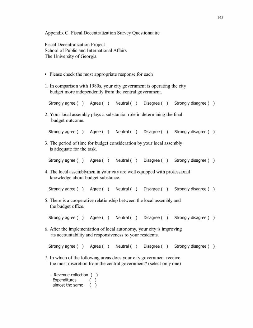
143

Appendix C. Fiscal Decentralization Survey Questionnaire Fiscal Decentralization Project School of Public and International Affairs The University of Georgia • Please check the most appropriate response for each 1. In comparison with 1980s, your city government is operating the city budget more independently from the central government. Strongly agree ( ) Agree ( ) Neutral ( ) Disagree ( ) Strongly disagree ( ) 2. Your local assembly plays a substantial role in determining the final budget outcome. Strongly agree ( ) Agree ( ) Neutral ( ) Disagree ( ) Strongly disagree ( ) 3. The period of time for budget consideration by your local assembly is adequate for the task. Strongly agree ( ) Agree ( ) Neutral ( ) Disagree ( ) Strongly disagree ( ) 4. The local assemblymen in your city are well equipped with professional knowledge about budget substance. Strongly agree ( ) Agree ( ) Neutral ( ) Disagree ( ) Strongly disagree ( ) 5. There is a cooperative relationship between the local assembly and the budget office. Strongly agree ( ) Agree ( ) Neutral ( ) Disagree ( ) Strongly disagree ( ) 6. After the implementation of local autonomy, your city is improving its accountability and responsiveness to your residents. Strongly agree ( ) Agree ( ) Neutral ( ) Disagree ( ) Strongly disagree ( ) 7. In which of the following areas does your city government receive the most discretion from the central government? (select only one) - Revenue collection ( ) - Expenditures ( ) - almost the same ( )

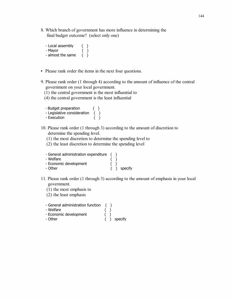
144

8. Which branch of government has more influence in determining the final budget outcome? (select only one) - Local assembly ( ) - Mayor ( ) - almost the same ( ) • Please rank order the items in the next four questions. 9. Please rank order (1 through 4) according to the amount of influence of the central government on your local government.

(1) the central government is the most influential to (4) the central government is the least influential

- Budget preparation ( ) - Legislative consideration ( ) - Execution ( ) 10. Please rank order (1 through 3) according to the amount of discretion to determine the spending level.

(1) the most discretion to determine the spending level to (2) the least discretion to determine the spending level

- General administration expenditure ( ) - Welfare ( ) - Economic development ( ) - Other ( ) specify 11. Please rank order (1 through 3) according to the amount of emphasis in your local government.

(1) the most emphasis to (2) the least emphasis

- General administration function ( ) - Welfare ( ) - Economic development ( ) - Other ( ) specify

145

12. Please rank order (1 through 8) according to the amount of discretion to determine the rate.

(1) the most discretion to determine the rate to (2) the least discretion to determine the rate

- Property rent ( ) - User charge ( ) - Fee ( ) - Inhabitant tax ( ) - Property tax ( ) - Automobile tax ( ) - Tobacco tax ( ) - Aggregate land tax ( ) - Other ( ) specify • Please write down your opinion. 13. What is the reason that �carry-over� occupies high share of local revenue? 14. Please provide any additional information concerning local autonomy and fiscal decentralization. ∗ Please return the completed questionnaire to the sender.

Thank you very much for your help.

146

Appendix D. Regression Estimations without Controlling Grant Effects

Table D.4.3. OLS Estimation of CE, LE, and TE (N=18) CE LE TE Intercept -0.705 -1.821 -0.762 (-6.559)*** (-19.668)*** (-6.335)*** DEC 0.237 2.539 1.1 (0.650) (8.077)*** (2.694)** R2 0.026 0.803 0.312 t-statistics in parentheses ** significant at the 5% level, two-tailed test; *** 1% Table D.4.4. OLS Estimation of CE, LE, AND TE with Control Variables (N=18) CE LE TE

Intercept -0.636 -1.983 -0.744 (-0.577) (-2.129)** (-0.610) DEC -2.316 0.274 -1.791 (-3.079)*** (0.430) (-2.150)** INCOME 1.004E-06 7.408E-07 1.095E-06 (1.383) (1.207) (1.363) POP 1.071E-08 1.550E-08 1.377E-08 (0.352) (0.603) (0.409) D-W 0.688 0.686 0.691 Adjusted R2 0.411 0.885 0.592 t-statistics in parentheses * significant at the 10% level, two-tailed test; ** 5%; *** 1%

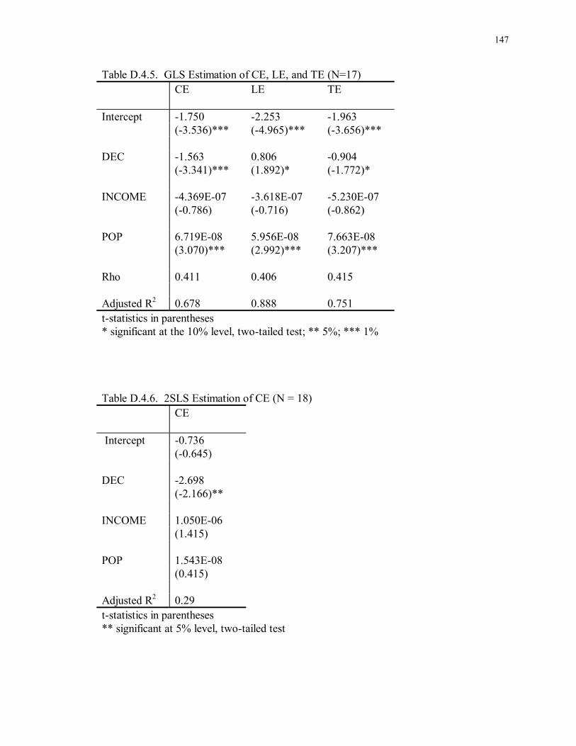
147

Table D.4.5. GLS Estimation of CE, LE, and TE (N=17) CE LE TE

Intercept -1.750 -2.253 -1.963 (-3.536)*** (-4.965)*** (-3.656)*** DEC -1.563 0.806 -0.904 (-3.341)*** (1.892)* (-1.772)* INCOME -4.369E-07 -3.618E-07 -5.230E-07 (-0.786) (-0.716) (-0.862) POP 6.719E-08 5.956E-08 7.663E-08 (3.070)*** (2.992)*** (3.207)*** Rho 0.411 0.406 0.415 Adjusted R2 0.678 0.888 0.751 t-statistics in parentheses * significant at the 10% level, two-tailed test; ** 5%; *** 1%

Table D.4.6. 2SLS Estimation of CE (N = 18) CE

Intercept -0.736 (-0.645) DEC -2.698 (-2.166)** INCOME 1.050E-06 (1.415) POP 1.543E-08 (0.415) Adjusted R2 0.29 t-statistics in parentheses ** significant at 5% level, two-tailed test

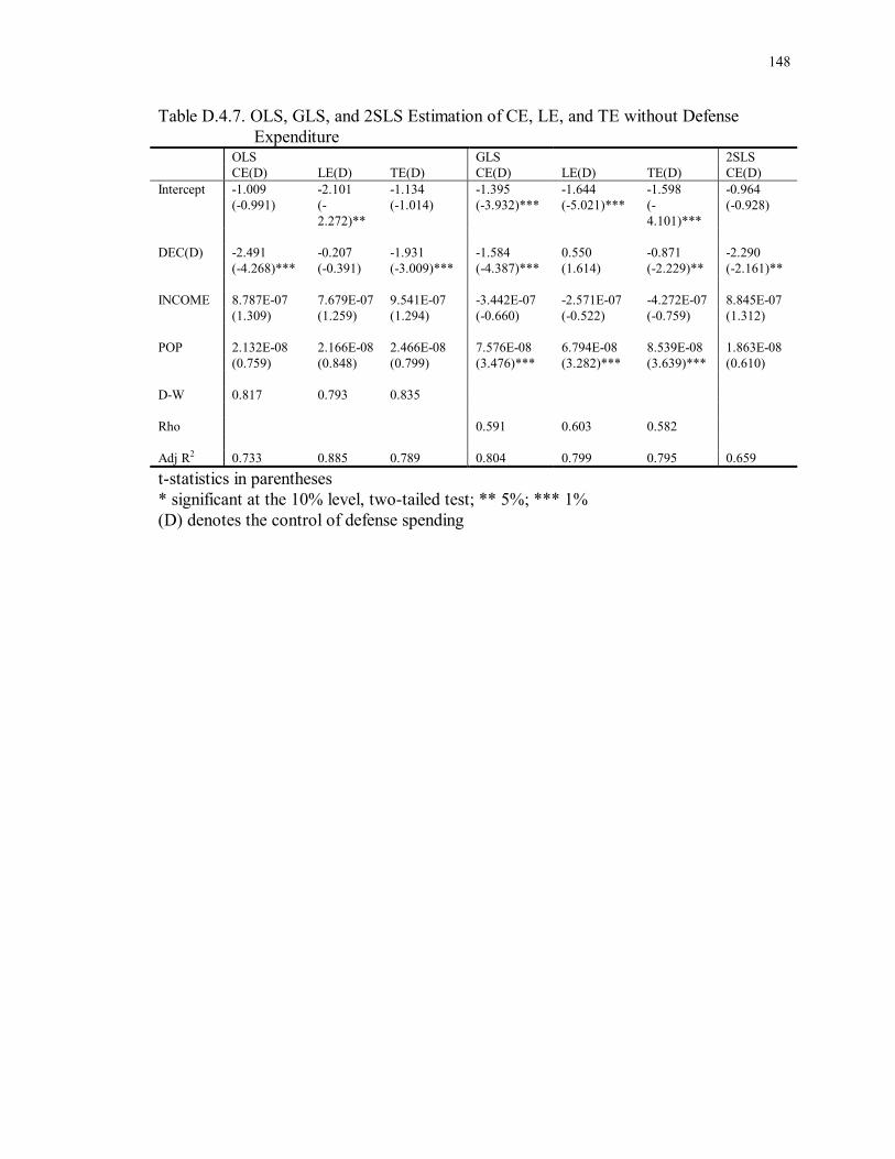
148

Table D.4.7. OLS, GLS, and 2SLS Estimation of CE, LE, and TE without Defense Expenditure OLS GLS 2SLS CE(D) LE(D) TE(D) CE(D) LE(D) TE(D) CE(D) Intercept -1.009 -2.101 -1.134 -1.395 -1.644 -1.598 -0.964 (-0.991) (-

2.272)** (-1.014) (-3.932)*** (-5.021)*** (-

4.101)*** (-0.928)

DEC(D) -2.491 -0.207 -1.931 -1.584 0.550 -0.871 -2.290 (-4.268)*** (-0.391) (-3.009)*** (-4.387)*** (1.614) (-2.229)** (-2.161)** INCOME 8.787E-07 7.679E-07 9.541E-07 -3.442E-07 -2.571E-07 -4.272E-07 8.845E-07 (1.309) (1.259) (1.294) (-0.660) (-0.522) (-0.759) (1.312) POP 2.132E-08 2.166E-08 2.466E-08 7.576E-08 6.794E-08 8.539E-08 1.863E-08 (0.759) (0.848) (0.799) (3.476)*** (3.282)*** (3.639)*** (0.610) D-W 0.817 0.793 0.835 Rho 0.591 0.603 0.582 Adj R2 0.733 0.885 0.789 0.804 0.799 0.795 0.659 t-statistics in parentheses * significant at the 10% level, two-tailed test; ** 5%; *** 1% (D) denotes the control of defense spending

149

REFERENCES Advisory Commission on Intergovernmental Relations (ACIR). 1964. The problem of special districts in American government. Washington, D.C.: Government Printing Office. Ahmad, Ehtisham, ed. 1997. Financing decentralized expenditures: An international comparison of grants. Cheltenham, U.K.: Edward Elgar. Bahl, Roy W. 1999. Fiscal decentralization as developmental policy. Public Budgeting & Finance 19, no. 2: 59-75. Bahl, Roy W., and J. Linn. 1992. Urban Public Finance in Developing Countries. New York: Oxford University Press. . 1994. Fiscal decentralization and intergovernmental transfers in less developed countries. Publius: The Journal of Federalism 24 (winter): 1-19. Bahl, Roy W., and S. Nath. 1986. Public expenditure decentralization in developing countries. Environment and Planning C: Government and Policy 4, no. 4: 405-418. Bahl, Roy W., and Robert J. Saunders. 1965. Determinants of changes in state and local government expenditures. National Tax Journal 18: 50-57. . 1966. Factors associated with variations in state and local government spending. Journal of Finance 21, no. 3: 523-534. Bahl, Roy W., and Walter Vogt. 1975. Fiscal centralization and tax burdens: State and regional financing of city services. Cambridge, M.A.: Ballinger Publishing Co. Bahl, Roy W., Marvin Johnson, and Michael Wasylenko. 1980. State and local government expenditure determinants: The traditional view and a new approach. In Public employment and state and local government finance. Roy Bahl, ed. Cambridge, M.A.: Ballinger Pub Co. Bartik, Timothy J. 1991. Who benefits from state and local development policies. Kalamazoo, M.I.: W.E. UpJohn Institute for Employment Research. Bartlett, Randall. 1973. Economic foundations of political power. New York: Free Press.

150

Bennett, Robert J. 1990. Decentralization, intergovernmental relations and markets: Towards a post-welfare agenda? In Decentralization, local governments, and markets. Bennett, ed. Oxford, U.K.: Clarendon Press. , ed. 1994. Local government and market decentralization: Experiences in industrialized, developing, and former Eastern bloc countries. Tokyo: United Nations University Press. Bird, R. M. 1993. Threading the fiscal labyrinth: Some issues in fiscal decentralization. National Tax Journal 46, no.2: 207-227. Bird, Richard M., and François Vaillancourt. 1998. Fiscal decentralization in developing countries: an overview. In Fiscal decentralization in developing countries. Bird, ed. Cambridge, U.K.: Cambridge University Press. Blank, Rebecca M. 1988. The effect of welfare and wage levels on the location decisions of female-headed households. Journal of Urban Economics 24, no. 2: 186-211. Bollens, John C. 1957. Special district governments in the United States. Berkeley; University of California Press. Borcherding, Thomas E., and Robert T. Deacon. 1972. The demand for the services of non-federal governments. The American Economic Review 62, no. 5:891-901. Bradford, David F., and W.E. Oates. 1974. Suburban exploitation of central cities and governmental structure. In Redistribution through public choice. Hochman and Peterson, eds. New York: Columbia University Press. Brennan, Geoffrey, and James M. Buchanan. 1980. The power to tax: Analytical foundations of a fiscal constitution. Cambridge, U.K.: Cambridge University Press. Breusch, T. S., and A. R. Pagan. 1980. The Lagrange multiplier test and its applications to model specification in econometrics. Review of Economic Studies 47: 239-253. Carlton, Dennis. 1983. The location and employment choices of new firms: An econometric model with discrete and continuous endogenous variables. The Review of Economics and Statistics 65, no. 3: 440-449. Choi, Kwang, and Soonwon Kwon. 1997. Social welfare and distribution policies. In The Korean economy 1945-1995: Performance and vision for the 21st century. Dong-Se Cha, Kwang-Suk Kim, and Dwight Perkins, eds. Seoul: Korea Development Institute. Davis, Otto, M. Dempster, and A. Wildavsky. 1966. A theory of the budgetary process. American Political Science Review 60, no. 3: 529-547.

151

Davoodi, Mamid, and Heng-fu Zou. 1998. Fiscal decentralization and economic growth: A cross-country study. Journal of Urban Economics 43, no. 2: 244-257. Dielman, Terry. 1989. Pooled cross-sectional and time series data analysis. New York: Marcel Dekker. Downs, Anthony. 1960. Why government is too small in a democracy. World Politics 12, no. 4: 541-563. Due, John F. 1961. Studies of state-local tax influence on location of industry. National Tax Journal 14: 163-173. Eberts, Randall W., and Timothy J. Gronberg. 1988. Can competition among local governments constrain government spending? Economic Review: Federal Reserve Bank of Cleveland 24, no. 1: 2-9. Fabricant, Solomon. 1952. The trend of government activity in the United States since 1900. Washington, D.C.: National Bureau of Economic Research. Fisher, Glenn W. 1961. Determinants of state and local governments expenditures: A preliminary analysis. National Tax Journal 14: 349-355. Fisher, Ronald C. 1996. State and local public finance. Chicago: IRWIN. Forbes, Kevin F., and Ernest M. Zampelli. 1989. Is Leviathan a mythical beast? The American Economic Review 79, no. 3: 568-577. Fukasaku, Kiichiro, and Luiz R. de Mello Jr., eds. 1999. Fiscal decentralization in emerging economies: Governance issues. Paris: OECD. Giertz, J. F. 1976. Decentralization at the state and local level: an empirical analysis. National Tax Journal 29, no. 2: 201-209. Glendening, Paris N., and Mavis Mann Reeves. 1984. Pragmatic federalism: An intergovernmental view of American government. Pacific Palisades, C.A.: Palisades Publishers. Goodspeed, Timothy. 1989. A re-examination of the use of ability to pay taxes by local governments. Journal of Public Economics 38, no. 3: 319-342. Gramlich, Edward M. 1977. Intergovernmental grants: A review of the empirical literature. In The political economy of fiscal federalism. Oates, ed. Lexington, M.A.: Heath-Lexington.

152

. 1987. Subnational fiscal policy. In Perspectives on local public finance. Quigley, ed. London: JAI Press. Gramlich, Edward M., and Deborah S. Laren. 1984. Migration and income redistribution responsibilities. Journal of Human Resources 29, no. 4: 489-511. Grodzins, Morton. 1966. The American system. In The American system: A new view of government in the United States. Elazar, ed. Chicago: Rand McNally. Grossman, Philip J. 1989. Fiscal decentralization and government size: An extension. Public Choice 62, no. 1: 63-70. .1992. Fiscal decentralization and public sector size in Australia. The Economic Record 68, no. 202: 240-246. Grossman, Philip J., and Edwin G. West. 1994. Federalism and the growth of government revisited. Public Choice 79, no. 1: 19-32. Gujarati, Damodar N. 1995. Basic econometrics. New York: McGraw-Hill. . 1999. Essentials of econometrics. New York: McGraw-Hill. Ha, Yeon-Seob. 1997. Public finance and budgeting in Korea under democracy: A critical appraisal. Public Budgeting & Finance 17, no. 1: 56-73. Hausman, J. A. 1978. Specification tests in econometrics. Econometrica 46, no. 6: 1251-1271. Heil, James B. 1991. The search for Leviathan revisited. Public Finance Quarterly 19, no. 3: 334-346. Homer, Martin. 1975. Economic and political causes of the welfare crisis. Unpublished Ph.D. Dissertation, MIT. Hsiao, Cheng. 1986. Analysis of panel data. Cambridge,U.K.: Cambridge University Press. Hyman, David N. 1993. Modern microeconomics: Analysis and applications. Homewood, I.L.: IRWIN. Joulfaian, David, and Michael L. Marlow. 1990. Government size and decentralization: Evidence from disaggregated data. Southern Economic Journal 56, no. 4: 1094-1102. Jun, Sang-Kyung. 1992. Intergovernmental fiscal relations. In Public finance in Korea. Choi, ed. Seoul: Seoul National University Press.

153

Kee, W. S. 1977. Fiscal decentralization and economic development. Public Finance Quarterly 5, no. 1: 79-97. Kemp, Kathleen. 1982. Instability in budgeting for federal regulatory agencies. Social Science Quarterly 63, no. 4: 643-660. Kenyon, Daphne A., and John Kincaid, eds. 1991. Competition among states and local governments: Efficiency and equity in American federalism. Washington, D.C.: The Urban Institute Press. Kim, Jong-Soon. 1997. Local Finance. Seoul: Sam-Young-Sa (Korean). Kim, Sang Loh. 1995. Fiscal decentralization, fiscal structure, and economic performance: Three empirical studies. Unpublished Ph.D. Dissertation, The University of Maryland. Kmenta, J. 1997. Elements of Econometrics. New York: Macmillan. Kneebone, Ronald D. 1992. Centralization and the size of government in Canada. Applied Economics 24, no. 12: 1293-1300. Korean Overseas Information. 1979. A handbook of Korea. Seoul: Ministry of Culture and Information. Kwack, Taewon. 1992. Size and structure of public expenditure. In Public Finance in Korea. Choi, ed. Seoul: Seoul National University Press. Kwon, Hyung-shin, Sang-yong Lee, and Jae-sung Lee. 1998. Local finance in Korea: Theory and practice. Seoul: Hae-Nam Press (Korean). Ladd, Helen F., and John Yinger. 1989. America�s ailing cities: Fiscal health and the design of urban policy. Baltimore: The Johns Hopkins University Press. Lauth, Thomas P. 1978. Zero-base budgeting in Georgia state government: Myth and reality. Public Administration Review38, no. 5: 420-430. Lauth, Thomas P. and James W. Douglas. 1995. Fiscal dependence of local governments in the United States: Changing patterns of fiscal federalism. Korean Public Administration Review 4, no. 4: 145-164. Leach, Richard H. 1970. American federalism. New York: W. W. Norton. Lee, Hyo. 1997. A study of resource allocation between the central and local governments. Seoul: Institute of Local Public Administration. (Korean)

154

Lee, Joon-Koo, and Sang-Dal Shim. 1992. The social welfare system. In Public finance in Korea. Choi, ed. Seoul: Seoul National University Press. Lee, Kye-Sik. 1987. Intergovernmental fiscal system and revenue distribution. Seoul: Korea Development Institute (Korean). Lee, Kye-Sik, Jong-Gu Park, and Yeon-Cheon Oh. 1990. Regional Development and Local Finance Seoul: Korea Development Institute. Lee, Yong-Jo, and Suk-Tae Kim. 1990. An empirical study on distribution methods of local share tax. Local and Administrative Study 2, no. 1: 99-119 (Korean). Levine, Philip B., and David J. Zimmerman. 1995. An empirical analysis of the welfare magnet debate using the NLSY. NBER working paper no. 5264. Cambridge, M.A.: National Bureau of Economic Research. Lim, Seong-il. 1997. Measuring the fiscal capacity of local governments. Seoul: Institute of Local Public Administration (Korean). Marlow, Michael L. 1988. Fiscal decentralization and government size. Public Choice 56, no. 3: 259-269. Mello, Luiz R. 2000. Fiscal decentralization and intergovernmental fiscal relations: A cross-country analysis. World Development 28, no. 2: 365-380. Mieszkowski, Peter, and Eric Toder. 1983. Taxation of energy resources. In Fiscal Federalism and the Taxation of Natural Resources. McLure and Mieszkowski, eds. Lexington, M.A.: Heath. Mikesell, John L. 1995. Fiscal administration: Analysis and applications for the public sector. Belmont, C.A.: Wadsworth Publishing Co. Moffit, R. 1992. Incentive effects of the US welfare system: A review. Journal of Economic Literature 30, no. 1: 1-61. Musgrave, Richard. 1959. The theory of public finance: A study in public economy. New York: McGraw-Hill. . 1983. Who should tax, where, and what? In Tax assignment in federal countries. McLure, ed. Canberra: Australian National University Press. Musgrave, Richard, and P. Musgrave. 1989. Public finance in theory and practice. New York: McGraw-Hill.

155

Musso, Juliet Ann. 1998. Fiscal federalism as a framework for governance reform. In Handbook of Public Finance. Thompson and Green, eds. New York: Marcel Dekker. Neck, Reinhard, and Friedrich Schneider. 1988. The growth of the public sector in Austria: An exploratory analysis. In Explaining the growth of government. Lybeck, ed. Amsterdam: North-Holland. Nelson, M. A. 1986. An empirical analysis of state and local tax structure in the context of the Leviathan model of government. Public Choice 49, no. 3: 283-294. . 1987. Searching for Leviathan: comment and extension. The American Economic Review 77, no. 1: 198-204. Netzer, Dick. 1991. An evaluation of interjurisdictional competition through economic development incentives. In Competition among states and local governments. Kenyon and Kincaid, eds. Washington, D.C.: The Urban Institute Press. Niskanen, William A. 1971. Bureaucracy and representative government. Chicago: Aldine Atherton. Noto, Nonna A. 1991. Trying to understand the economic development official�s dilemma. In Competition among states and local governments: Efficiency and equity in American federalism. Kenyon and Kincaid, eds. Washington, D.C.: The Urban Institute Press. Oates, Wallace E. 1972. Fiscal Federalism. New York: Harcourt Brace Jovanovich. . 1977. An economist�s perspective on fiscal federalism. In The political economy of fiscal federalism. Oates, ed. Lexington, M.A.: Lexington Books. . 1985. Searching for Leviathan: An empirical study. The American Economic Review 75, no. 4: 748-757. . 1994. Federalism and government finance. In Modern public finance. Quigley and Smolensky, eds. Cambridge, M.A.: Harvard University Press. . 1999. An essay on fiscal federalism. Journal of Economic Literature 37: 1120-1149. Oates, Wallace E., and Robert Schwab. 1991. The allocative and distributive implications of local fiscal competition. In Competition among states and local Governments: Efficiency and equity in American federalism. Kenyon and Kincaid, eds. Washington, D.C.: The Urban Institute Press. Oh, Heu-Hwan, and Kee-Kwan Park. 1996. A study of user charges and fees in Korea. Seoul: Institute of Local Public Administration (Korean).

156

Oh, Yeon-Cheon. 1992a. Korean tax system. Seoul: Pak-Young-Sa (Korean). . 1992b. The local tax system. In Public finance in Korea. Choi, ed. Seoul: Seoul National University Press. Panizza, Ugo. 1999. On the determinants of fiscal centralization: theory and evidence. Journal of Public Economics 74, no. 1: 97-139. Park, Jong Koo. 1992. Special accounts and public funds. In Public finance in Korea. Choi, ed. Seoul: Seoul National University Press. Park, R. E. 1966. Estimation with heteroscedastic error terms. Econometrica 34, no. 4: 888. Pauly, Mark V. 1973. Income redistribution as a local public good. Journal of Public Economics 2, no. 1: 33-58. Peacock, Allen T. 1979. The economic analysis of government and related themes. Oxford, U.K.: Martin Robertson. Peacock, Allen T., and J. Wiseman. 1961. The growth of government expenditures in the United Kingdom. Princeton: Princeton University Press. Perrenod, Virginia M. 1984. Special districts, special purpose: Fringe governments and urban problems in the Houston area. College Station: Texas A&M University Press. Peterson, Paul E. 1979. A unitary model of local taxation and expenditure policies in the United States. British Journal of Political Science 9, no. 3: 281-314. . 1981. City limits. Chicago: The University of Chicago Press. . 1995. The price of federalism. Washington, D.C.: The Brookings Institution. Peterson, Paul E. and M. Rom. 1990. Welfare magnets: The case for a national welfare standard. Washington, D.C.: The Brookings Institution. Prud�homme, Remy. 1990. Decentralization of expenditures or taxes: The case of France. In Decentralization, local governments, and markets. Bennett, ed. Oxford, U.K.: Clarendon Press. . 1995. The dangers of decentralization. The World Bank Research Observer 10, no. 2: 201-220. Raimondo, Henry J. 1992. Economics of state and local government. New York: Praeger.

157

Rivlin, Alice M. 1992. Reviving the American dream: The economy, the states & the federal government. Washington, D.C.: The Brookings Institution. Sacks, Seymour, and Robert Harris. 1964. The determinants of state and local government expenditures and intergovernmental flows of funds. National Tax Journal 17: 75-85. Schick, Allen. 1983. Incremental budgeting in a decremental age. Policy Sciences 16, no. 1: 1-25. Shadbegian, Ronald J. 1999. Fiscal federalism, collusion, and government size: Evidence from the states. Public Finance Review 27, no. 3: 262-281. Smith, Roger S., and Chong-In Kim. 1979. Local finances in non-metropolitan cities of Korea. In Urban and Regional Report. ed. Washington, D.C.: World Bank. Sorensen, Rune J. 1988. The growth of public spending in Norway 1865-1985: The impact of political mobilization, macroeconomic situations and government popularity. In Explaining the Growth of Government. Lybeck, ed. Amsterdam: North-Holland. Stimson, James A. 1985. Regression in space and time: a statistical essay. American Journal of Political Science 29, no. 4: 914-947. Tiebout, C. 1956. A pure theory of local public expenditure. Journal of Political Economy 64, no. 5: 416-424. Walker, James R. 1994. Migration among low-income households: Helping the witch doctors reach consensus. IRP working paper no. 1031-94. Madison, W.I.: Institute for Research on Poverty. Wallis, John Joseph, and Wallace Oates. 1988. Decentralization in the public sector: An empirical study of state and local government. In Fiscal Federalism: Quantitative Studies. Rosen, ed. Chicago: The University of Chicago Press. Wasylenko, Michael. 1987. Fiscal decentralization and economic development. Public Budgeting & Finance 7, no. 4: 57-71. Weimer, David L., and Aidan R. Vining. 1992. Policy analysis: Concepts and practice. Englewood Cliffs, N.J.: Prentice Hall. Wildavsky, Aaron. 1986. Budgeting: A comparative theory of budgetary processes. New Brunswick, N.J.: Transaction Books. Wolman, Hal, and Sharon McCormick. 1994. The effect of decentralization on local governments. In Local government and market decentralization. Bennett, ed. Tokyo: United Nations University Press.

158

Yoo, Hoon. 1998. Local Public Finance. Seoul: Bub-Moon-Sa (Korean). Zax, Jeffrey S. 1989. Is there a Leviathan in your neighborhood? The American Economic Review 79, no. 3: 560-567. Zorn, Kurt C. 1991. User charges and fees. In Local government finance: Concepts and practices. Petersen and Strachota, eds. Chicago: Government Finance Officers Association.

THE EFFECTS OF FISCAL DECENTRALIZATION ON LOCAL …

Documents

Transcript of THE EFFECTS OF FISCAL DECENTRALIZATION ON LOCAL …