The Effect of Turbulence Modelling on theAssessment of Platelet ActivationSilvia Bozzi  ( silvia.bozzi@polimi.it )

Polytechnic University of MilanDavide Dominissini 

Polytechnic University of MilanAlberto Redaelli 

Polytechnic University of MilanGiuseppe Passoni 

Polytechnic University of Milan

Research Article

Keywords: Platelet activation, Mechanical heart valves, Turbulence, CFD models, DNS, LES, RANS

Posted Date: December 18th, 2020

DOI: https://doi.org/10.21203/rs.3.rs-129700/v1

License: This work is licensed under a Creative Commons Attribution 4.0 International License.  Read Full License

Version of Record: A version of this preprint was published at Journal of Biomechanics on November 1st,2021. See the published version at https://doi.org/10.1016/j.jbiomech.2021.110704.

The effect of turbulence modelling on the assessment of platelet activation

Silvia Bozzi1* · Davide Dominissini1 · Alberto Redaelli1 · Giuseppe Passoni1 1 Politecnico di Milano, Department of Electronics Information and Bioengineering, Milano, Italy

*Corresponding Author: Silvia Bozzi, silvia.bozzi@polimi.it

Abstract Pathological platelet activation induced by abnormal shear stresses is regarded as a main clinical complication

in recipients of cardiovascular biomedical implantable devices and prostheses. In order to improve their performance

computational fluid dynamics (CFD) has been used to evaluate flow fields and related shear stresses. More recently CFD

models have been equipped with mathematical models that describe the relation between fluid dynamics variables,

and in particular shear stresses, and the platelet activation state (PAS). These mathematical models typically use a

Lagrangian approach to extract the shear stresses along possible platelet trajectories. However, in the case of turbulent

flow, the choice of the proper turbulence closure model is still debated for both concerning its effect on Lagrangian

statistics and shear stress calculation. In our study five numerical simulations of the flow through a mechanical heart

valve were performed and then compared in terms of Eulerian and Lagrangian quantities: a direct numerical simulation

(DNS), a large eddy simulation (LES), two Reynolds-averaged Navier-Stokes (RANS) simulations (SST k- and RSM) and

a “Laminar” (no turbulence modelling on a Taylor microscale-based grid) simulation. Results exhibit a large variability

in the PAS assessment depending on the turbulence model adopted. “Laminar” and RSM estimates of platelet activation are about 60% below DNS, while LES is 16% less. Surprisingly, PAS estimated from the SST k- velocity field is only 8%

less than from DNS data. This appears more artificial than physical as can be inferred after comparing frequency

distributions of PAS and of the different Lagrangian variables of the mechano-biological model of platelet activation.

Our study indicates that turbulence closures can lead to a severe underestimation of platelet activation and suggests

that turbulence should be fully resolved by DNS when assessing blood damage in blood contacting devices.

Keywords Platelet activation · Mechanical heart valves · Turbulence · CFD models · DNS · LES · RANS

Introduction

It is well known that cardiovascular devices determine thromboembolic consequences for which anticoagulant therapy

is mandatory [1 – 4]. The phenomenon is triggered by blood-device interaction in terms of both chemical and mechanical

stimuli [5]. The exposure to higher and more discontinuous shear stresses, than in physiological situations, is per se a

sufficient condition to induce platelet activation and aggregation [6, 7]. Indeed, shear-mediated platelet activation

(SMPA) is often the driving factor for thrombotic complications in presence of anatomic pathologies and cardiovascular

devices [8 – 10].

In 2008 the United States Food and Drug Administration (FDA) launched a Critical Path initiative to assess the predictive

capability of computational fluid dynamics (CFD) simulations and blood damage models used to evaluate blood-

contacting medical devices [11]. This initiative led to the development of a specific FDA Guidance Document aimed at

regulating the use of CFD in the field of medical device assessment [12]. Nowadays, CFD is considered one of the type

of models to prove scientific evidence for medical regulatory decision-making (ISO 5840-2 2015); the continuous

advancement of CFD techniques allows for the simulation of the hemodynamics through complex medical devices, such

as ventricular assist devices (VAD) and mechanical heart valves (MHV) with an outstanding level of detail. CFD studies

have been also equipped with blood damage models, which allows to evaluate the hemocompatibility of blood-

contacting devices in terms of haemolysis and platelet. In particular, new numerical models [13, 14] have been

developed for the computation of the platelet activation state (PAS), due to flow shear stresses. These models are based

on the Lagrangian analysis of possible platelet trajectories along which flow field metrics involved in the process of

platelet activation are extracted. These models were initially based on the power law equation proposed by Giersiepen

et al. [15]. However, in 2008 we introduced the damage accumulation model [13] to account for platelet damage

accumulation, which has been lately improved to include the effect of stress rate [14]. Noteworthy, in a recent work we

have demonstrated that high frequency components in the shear stress history are a major determinant of the shear-

induced platelet activation [16]. The nonlinear structure of the PAS model equations implies that the accuracy of the

flow solution and the associated Lagrangian computations – especially close to geometric singularities – are of utmost

importance when computing platelet activation along the trajectories.

An extensive discussion on the different methodological aspects of the Lagrangian computations can be found in Marom

and Bluestein [17]. Conversely, the accuracy of fluid dynamics solutions is still an open issue, especially when dealing

with thrombotic risk assessment [18]. The reliability of CFD is crucial when dealing with fluid dynamics in large vessels,

like aorta, where typical Reynolds numbers entail simulating a hierarchy of flow structures [19]. Due to the

computational cost of the direct numerical simulation (DNS), the so-called Reynolds-averaged Navier-Stokes (RANS)

simulations have been and still remain the most common approach for turbulent flows in complex geometries. Despite

their long history [20] turbulence closures are essentially based on empirical relations whose parameters require

problem-dependent calibrations. The choice among different turbulence closures is still an open issue since most of

them are accurate for the average flow characteristics only, while for shear stress and its derivatives this is much more

uncertain, especially when calculations are cast in a Lagrangian framework. In many biomechanical flows, nonlinearities

and turbulent closures have been shown to be crucial [21, 22], especially when dealing with higher order moments of

the velocity [23, 24]. Recently, an interesting analysis has been presented by Pal et al. [25] but limited to the large eddy

simulation (LES) closure models and to the fluid dynamics variables. As a matter of fact, the effects of the different

types of turbulence closures (RANS, LES and DNS) on the resulting Lagrangian statistics and on the platelet activation

state have not yet been ascertained. Indeed, shear stresses are calculated differently depending on the turbulent

closure model, thus the model choice strongly affects the quantification of the thrombogenic potential.

In this paper we show how different turbulence models affect the flow solution around and paste a bileaflet mechanical

heart valve (BMHV) and how the differences in the Eulerian fields are mapped onto Lagrangian statistics and platelet

activation. Five numerical simulations have been performed: a direct numerical simulation, a large eddy simulation, two

Reynolds-averaged Navier-Stokes simulations and a laminar (no turbulence modelling) simulation. These models were

compared in terms of Eulerian fields, such as blood velocity and fluid stresses and Lagrangian quantities, such as stress

accumulation and stress rate and finally in terms of platelet activation state.

Methods

Turbulence causes the formation of eddies with a wide range of time and length scales, that interact with each other

and with the mean flow in a dynamically complex way. Numerical methods for turbulent flow calculations can be divided

into three categories: turbulence models for the Reynolds-averaged Navier-Stokes equations, large eddy simulation and

direct numerical simulation.

In RANS equations, the Reynolds decomposition of the velocity field results in an extra tensor - Reynolds stress, i.e. the

correlation among fluctuating velocity components - for which extra equations are necessary. Starting from the

Boussinesq’s eddy viscosity concept many models were derived like k-ε [26] and k- [27], where turbulent viscosity is

related to turbulent kinetic energy (k) and turbulent dissipation rate (ε), or specific dissipation rate (ω), respectively. A

combination of the two previous models was later proposed by Menter [28]: the SST (Shear Stress Transport) k- model,

which uses the k- model close to the wall and the k-ε in the inner region. Finally, Hanjalic and Launder [29] introduced

the so-called Reynolds Stress Model (RSM), which is the most complex RANS turbulence model involving the calculation

of the six individual components of the Reynolds stress tensor.

A different approach was proposed by Smagorinsky [30] in the so-called large eddy simulation. Starting from

Kolmogorov’s theory (see e.g. [31]), the idea was to explicitly solve the large eddies, leaving the smallest dissipative

ones to a model. LES uses a convolution filter operator to separate the subgrid scale (SGS) motion (i.e. the smallest

unresolved eddies) from larger eddy structures. As a result, the nonlinear acceleration terms in the Navier-Stokes

equations give rise to sub-grid-scale stresses called SGS stresses, which are modelled by a turbulence model combined

with a proper formulation for turbulent viscosity. SGS stress tensor and turbulent viscosity have different formal

structures with respect to RANS models, as the filter operators are different.

DNS consists in the numerical integration of the Navier-Stokes equations with enough accuracy in space and time to

capture even the smallest dissipative flow structures. This results in extremely demanding numerical computations,

being the number of degrees of freedom (i.e. nodal points in the space directions) proportional to 𝑅𝑒9 4⁄ [32], with 𝑅𝑒

equal to the Reynolds number, defined as 𝑅𝑒 = 𝑈𝐿 𝜈⁄ , where 𝑈 and 𝐿 are a characteristic velocity and length scale,

respectively and 𝜈 is the kinematic viscosity of the fluid.

Nowadays, RANS are the most widely used turbulence models by the CFD community because most of the engineering

applications are only interested in the mean flow and in the effects of turbulence on the mean flow properties. However,

they fail in simulating complex engineering flows, such as flows with adverse pressure gradients, significant streamline

curvature and stagnation regions. In such cases, LES models offers much better accuracy and even if they require large

computation resources, they are now starting to address complex problems. Finally, DNS presents the most accurate

method for turbulent flow simulations, but due to the high computation cost it is limited to low Reynolds number flows

and simple geometries.

As reported in the Introduction section we have focused our analysis on five different turbulent models characterized

by different levels of accuracy: (1) a robust isotropic RANS turbulent closure (SST k- ), which performs well in confined

flows and in presence of bluff bodies (such as cardiac valves), (2) an anisotropic RANS model, which accounts for the

directional effects of the Reynolds stresses, (3) a LES model which can provides not only information on the mean flow,

but also certain time dependent features of the resolved fluctuations and (4) a DNS approach which represents the

closest solution to the real flow field. Moreover, we also performed a “laminar” simulation, i.e. a Navier Stokes

integration, without any turbulence closure, on a grid larger than that required to fully solve all the turbulent eddies.

This simulation can provide an insight on the effects of an insufficient grid resolution, which is a main issue when low

Reynolds flows are solved without turbulent closures.

Geometrical modelling

The mechanical valve used in the simulations is the Sorin Bicarbon Fitline Size 25, produced by Sorin (now LivaNova,

Cardiac Surgery Unit). The geometrical model of the valve was created with ANSYS® SpaceClaim 18.2 starting from the

CAD drawing of the valve provided by the manufacturer. The two leaflets were considered fully opened since this

configuration is maintained for a considerable time window around the velocity peak [24, 33, 34]. The small hinge

mechanism was modelled with two intercepting spherical caps of radius 4.5 mm. This artificial gap size (320 m) is

larger than the real one (≈ 240 m). This choice was adopted to mesh the gap with at least 10 cells, thus obtaining a

high quality mesh and minimizing computational problems [35].

The BMHV was placed between two cylindrical straight tubes, with a diameter of D = 22 mm, to mimic a standard mock

loop set-up (Fig. 1a). After a sensitivity analysis the entry region was set equal to 2D while the tube past the valve was

extended to 5D, to achieve a fully developed flow at the outlet section.

Downstream the valve, the three aortic sinuses were sketched as prolate spheroids with major axis of 22 mm, oriented

in x–direction, and minor axis of 20 mm, in both y– and z–direction. Their interception with the tube (i.e. the height of

the sinus) measures HSTJ = 18.75 mm and their maximum width is WM = 5.5 mm. Moreover, their position is radial–symmetric in the plane orthogonal to the streamwise direction.

Mesh generation

Different grids for the fluid domain were created for the five simulations. RANS and “laminar” simulations were performed on the same mesh (Fig. 1b), based on the Taylor microscale 𝜆, defined as:

𝜆 ≔ 𝐷 (10𝑅𝑒)1/2 (1)

where 𝑅𝑒 is the Reynolds number, calculated considering the average inlet velocity at the systolic peak and the tube

diameter. This grid size resulted from a mesh convergence study, which compared three mesh refinements using the

grid convergence index (GCI) method [36]. The boundary layer was discretized with a first cell size of 𝑦+ = 1, a grow

rate of 1.15 in the wall-normal direction and a total thickness of 1.33 mm, estimated on the basis of the value of

turbulence intensity.

The LES mesh was built with a characteristic dimension of 16 𝜂, being 𝜂 the Kolmogorov microscale:

𝜂 = 𝐷𝑅𝑒−3/4 (2)

DNS was performed on a finer mesh with a characteristic size of 8𝜂, able to catch large part of the whole energy cascade

[37]. The Kolmogorov length scale is commonly quoted as the smallest scale to be resolved in a direct simulation.

However, as most of the dissipation takes place at scales larger than 𝜂, the smallest resolved length scale has to be of

the order of 𝜂 and not exactly 𝜂 [38]. The boundary layers of LES and DNS were discretized placing the first cell centre

at 𝑦+ = 0.1 and 𝑦+ = 0.05 respectively and using a grow rate factor of 1.15.

The total number of elements resulted in about 3.3 million cells for RANS and “laminar” simulations, 9.3 million for LES

and 54 million for DNS. Other DNS studies [34, 39] used 9.7 and 6.6 million grid points, respectively. The main

parameters of the three meshes are reported in Table 1.

Numerical approach

Blood was assumed incompressible and Newtonian with density 𝜌 = 1060 kg m-3 and dynamic viscosity =0.0035 𝑃𝑎 ∙𝑠. The flow field was computed solving the 3D, unsteady, incompressible continuity and momentum equations:

∇ ∙ 𝒖 = 0 (3) 𝜌 𝐷𝒖𝐷𝑡 = −∇𝑝 + 𝜇∇2𝒖 (4)

where 𝒖 is the velocity vector, 𝑝 the isotropic pressure, 𝜌 and 𝜇 the fluid density and dynamic viscosity, respectively. 𝐷/𝐷𝑡 is the material derivative defined as 𝐷𝑩 ∕ 𝐷𝑡 ≔ 𝜕𝑩/𝜕𝑡 + (𝒖 ∙ ∇)𝑩, being 𝑩 a general tensor field.

The commercial software ANSYS® Fluent 19.1 was used for the numerical simulations, where the finite volume method

(FVM) is used for the space discretization of the system of partial differential equations (PDEs). In the simulations the

SIMPLE algorithm was adopted for pressure and velocity coupling and a 2nd order scheme for spatial derivatives. In

particular, a least squares cell-based method was used for the gradients and a second order upwind method for pressure

and momentum equations. In RANS simulations a 2nd order upwind method was employed for the turbulent kinetic

energy k and the specific dissipation rate . Default ANSYS® Fluent constants were used for all the turbulent models

(SST k- RSM and LES) and a low-Re correction was selected for the SST k- closure. For time derivatives a 1st order

implicit formulation was used. All the simulations were performed with a convergence criterion of 10-4 for the residual

errors.

The simulated transient was limited to the systolic phase, having a duration of 290 ms. The Eulerian and Lagrangian

analysis were limited within the interval between 36 ms and 231 ms, i.e. the time of maximum acceleration (A) and

deceleration (D) before and after the systolic peak (P) (Fig. 2), respectively. After a sensitivity analysis, a time step equal

to 1 ms was set for RANS and “laminar” simulations, while LES and DNS were performed using a time step of 0.25 ms and 0.1 ms, respectively.

A fully developed parabolic velocity profile was imposed as inlet boundary condition with a maximum cross-section

velocity mimicking a physiological systolic waveform (Fig. 2). The resulting inlet Reynolds number (based on the

maximum cross-section velocity magnitude and tube diameter) were 2800, 8900 and 4400 for the instants of maximum

acceleration, systolic peak and maximum deceleration, respectively. This indicates that during the systolic phase the

flow regime varies from laminar through transitional to low Re turbulent. Constant pressure was prescribed at the

outlet and a no–slip condition was imposed at the walls.

Platelet injection

In order to simulate the platelets dynamics through the BMHV, 11347 neutrally buoyant spherical particles (diameter 3

m) were released in the fluid domain. They were injected instantaneously at 𝑡 = 112 ms, on a plane 𝑦𝑧 located 1D

upstream the leaflets. The injection time and position were set so that at the systolic peak 90% of the platelets were

crossing the valve plane (i.e. were between − 𝐷 2⁄ and +𝐷 2⁄ from the valve). A concentric circular seeding pattern was

implemented since it assures a constant distance from the wall and thus more accurate Lagrangian estimates of fluid

stresses [17]. A discrete particle model was used to track platelets, including drag force in the equation of motion and

a rebound condition for particles hitting the walls. Particles trajectories were extracted between − 𝐷 2⁄ and +3𝐷, with

respect to the valve, to exclude the entry tube, which is a numerical artefact, and to limit the influence of the outlet

condition. The platelets that had not left the domain at the end of the simulation were not considered.

Lagrangian analysis and PAS estimation

In order to determine the total stress acting on a platelet particle, the nine components of the stress tensor:

𝜏𝑖𝑗 = −𝜇 (𝜕𝑢𝑖𝜕𝑥𝑗 + 𝜕𝑢𝑗𝜕𝑥𝑖) (5)

were reduced to a single scalar value:

𝜎 = ( 112 (𝜏𝑖𝑖 − 𝜏𝑗𝑗)2 + 12 𝜏𝑖𝑗2 )1/2 (6)

This is a common procedure in literature, firstly presented by Bludszuweit [40] and then corrected by Faghih & Sharp

[41]. The quantity 𝜎 is referred to as the scalar stress or scalar total stress. Each value of 𝜏𝑖𝑗 represents a component of

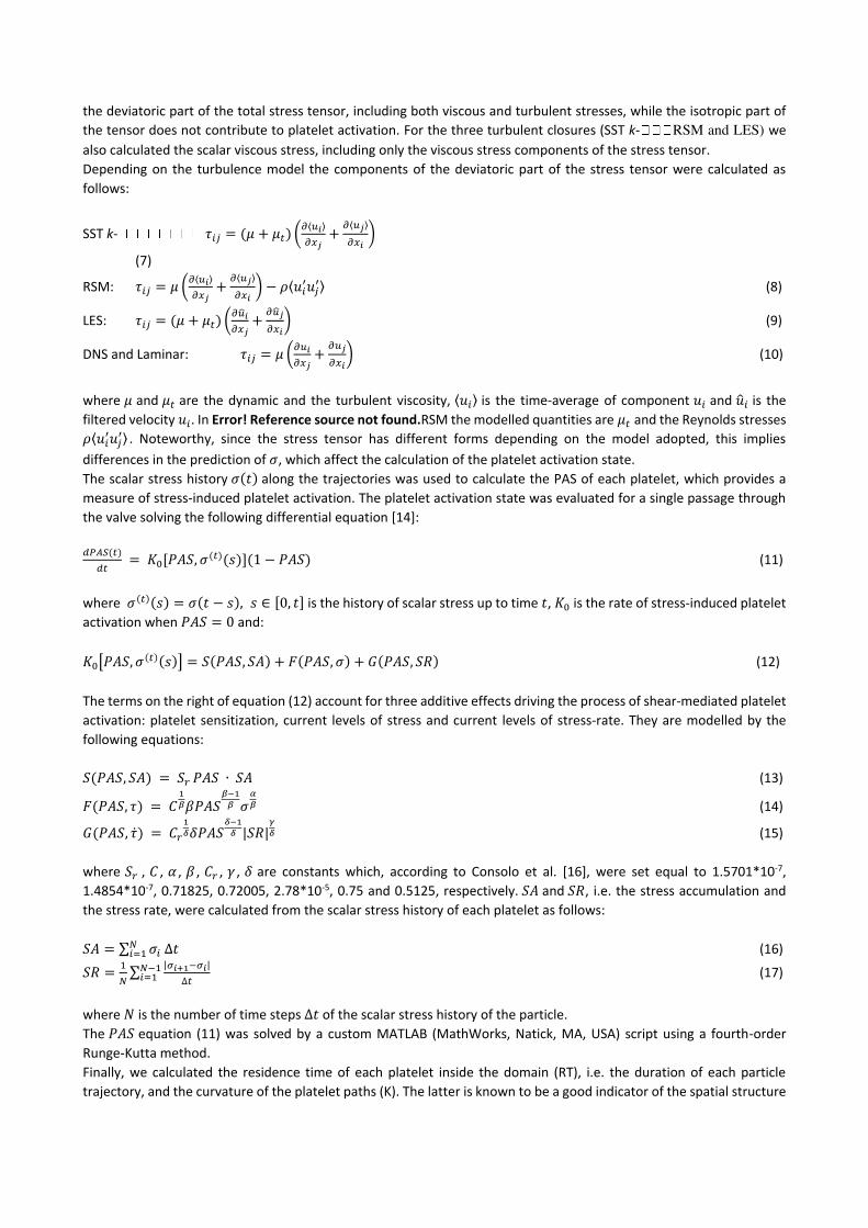
the deviatoric part of the total stress tensor, including both viscous and turbulent stresses, while the isotropic part of

the tensor does not contribute to platelet activation. For the three turbulent closures (SST k- RSM and LES) we

also calculated the scalar viscous stress, including only the viscous stress components of the stress tensor.

Depending on the turbulence model the components of the deviatoric part of the stress tensor were calculated as

follows:

SST k- 𝜏𝑖𝑗 = (𝜇 + 𝜇𝑡) (𝜕⟨𝑢𝑖⟩𝜕𝑥𝑗 + 𝜕⟨𝑢𝑗⟩𝜕𝑥𝑖 )

(7)

RSM: 𝜏𝑖𝑗 = 𝜇 (𝜕⟨𝑢𝑖⟩𝜕𝑥𝑗 + 𝜕⟨𝑢𝑗⟩𝜕𝑥𝑖 ) − 𝜌⟨𝑢𝑖′𝑢𝑗′⟩ (8)

LES: 𝜏𝑖𝑗 = (𝜇 + 𝜇𝑡) (𝜕�̂�𝑖𝜕𝑥𝑗 + 𝜕�̂�𝑗𝜕𝑥𝑖) (9)

DNS and Laminar: 𝜏𝑖𝑗 = 𝜇 (𝜕𝑢𝑖𝜕𝑥𝑗 + 𝜕𝑢𝑗𝜕𝑥𝑖) (10)

where 𝜇 and 𝜇𝑡 are the dynamic and the turbulent viscosity, ⟨𝑢𝑖⟩ is the time-average of component 𝑢𝑖 and �̂�𝑖 is the

filtered velocity 𝑢𝑖. In Error! Reference source not found.RSM the modelled quantities are 𝜇𝑡 and the Reynolds stresses 𝜌⟨𝑢𝑖′𝑢𝑗′⟩ . Noteworthy, since the stress tensor has different forms depending on the model adopted, this implies

differences in the prediction of 𝜎, which affect the calculation of the platelet activation state.

The scalar stress history 𝜎(𝑡) along the trajectories was used to calculate the PAS of each platelet, which provides a

measure of stress-induced platelet activation. The platelet activation state was evaluated for a single passage through

the valve solving the following differential equation [14]:

𝑑𝑃𝐴𝑆(𝑡)𝑑𝑡 = 𝐾0[𝑃𝐴𝑆, 𝜎(𝑡)(𝑠)](1 − 𝑃𝐴𝑆) (11)

where 𝜎(𝑡)(𝑠) = 𝜎(𝑡 − 𝑠), 𝑠 ∈ [0, 𝑡] is the history of scalar stress up to time 𝑡, 𝐾0 is the rate of stress-induced platelet

activation when 𝑃𝐴𝑆 = 0 and:

𝐾0[𝑃𝐴𝑆, 𝜎(𝑡)(𝑠)] = 𝑆(𝑃𝐴𝑆, 𝑆𝐴) + 𝐹(𝑃𝐴𝑆, 𝜎) + 𝐺(𝑃𝐴𝑆, 𝑆𝑅) (12)

The terms on the right of equation (12) account for three additive effects driving the process of shear-mediated platelet

activation: platelet sensitization, current levels of stress and current levels of stress-rate. They are modelled by the

following equations:

𝑆(𝑃𝐴𝑆, 𝑆𝐴) = 𝑆𝑟 𝑃𝐴𝑆 ∙ 𝑆𝐴 (13) 𝐹(𝑃𝐴𝑆, 𝜏) = 𝐶 1𝛽𝛽𝑃𝐴𝑆𝛽−1𝛽 𝜎𝛼𝛽 (14) 𝐺(𝑃𝐴𝑆, �̇�) = 𝐶𝑟 1𝛿𝛿𝑃𝐴𝑆𝛿−1𝛿 |𝑆𝑅|𝛾𝛿 (15)

where 𝑆𝑟 , 𝐶 , 𝛼 , 𝛽 , 𝐶𝑟 , 𝛾 , 𝛿 are constants which, according to Consolo et al. [16], were set equal to 1.5701*10-7,

1.4854*10-7, 0.71825, 0.72005, 2.78*10-5, 0.75 and 0.5125, respectively. 𝑆𝐴 and 𝑆𝑅, i.e. the stress accumulation and

the stress rate, were calculated from the scalar stress history of each platelet as follows:

𝑆𝐴 = ∑ 𝜎𝑖 ∆𝑡𝑁𝑖=1 (16) 𝑆𝑅 = 1𝑁 ∑ |𝜎𝑖+1−𝜎𝑖|∆𝑡𝑁−1𝑖=1 (17)

where 𝑁 is the number of time steps ∆𝑡 of the scalar stress history of the particle.

The 𝑃𝐴𝑆 equation (11) was solved by a custom MATLAB (MathWorks, Natick, MA, USA) script using a fourth-order

Runge-Kutta method.

Finally, we calculated the residence time of each platelet inside the domain (RT), i.e. the duration of each particle

trajectory, and the curvature of the platelet paths (K). The latter is known to be a good indicator of the spatial structure

of the velocity field [42, 43] and to play an important role in platelet activation [44]. As in Braun et al. [42] the following

definition of the local curvature was used:

𝜅 = |𝐮 x �̇�||𝐮|3 (18)

where 𝐮 is the velocity vector and the dot denotes the material derivative. For each particle, at each time step, the

curvature has been calculated discretizing equation (18) with a central differencing scheme and then the average

integral curvature was computed for each trajectory.

Results

Eulerian fields

The fluid dynamics solution of the five models was compared in terms of streamwise velocity profiles at the systolic

peak (Supplementary Fig. S1) and velocity and scalar stress contours at the three time instants A (Supplementary Fig.

S2 and S3), P (Fig. 3 and 4) and D (Supplementary Fig. S5 and S6). For the models including a turbulent closure (SST k-

RSM and LES), we also analysed the scalar viscous stress (Supplementary Fig. S4, Fig. 5 and Supplementary Fig. S7

for the instants A, P and D, respectively).

During the acceleration phase (A), the flow is essentially laminar, thus it is well represented by all the models employed

(Supplementary Fig. S2 and S3). However, when the systole reaches its peak, the flow downstream the valve “explodes” in complex and smaller structures (Fig. 3) that can be caught only with scale-resolving simulations (LES and DNS).

Differences emerge downstream the valve where the shear layer of the leaflets detaches from the leaflets tips and

higher turbulence occurs (Supplementary Fig. S1, from (c) to (f)), whereas the velocity profile at the valve is almost the

same for all the simulations (Supplementary Fig. S1 (a) and (b)). The typical triple jet nature of the flow can be also

appreciated (e.g. [45]). The scalar stress contours (Fig. 4) show that the highest fluid stresses occur in the leaflet

boundary layer, in the wake of the valve and in the sinuses. Fluid stresses are more affected by the turbulence model

than the resolved velocity field, as expected considering that they are computed upon derivatives of the velocity vector.

Differences emerges even among the RANS approaches: the RSM predicts scalar stress values of the same of order of

magnitude of the DNS, while the SST k- overestimates the stresses by one order of magnitude. Integral quantities are

well predicted by all the turbulence models: at the systolic peak the maximum streamwise velocity near the valve ranges

between 1.92 and 1.98 m/s and the pressure drop varies from 600 to 673 Pa, depending on the simulation (Table 2).

This result is as expected, since mean flow properties are known to be correctly estimated both by turbulence models

based on the Reynolds decomposition [37] and laminar models [46]. During the deceleration phase of systole, the flow

past the valve exhibits a complex topology induced by a periodic vortex shedding in the wave of the leaflets

(Supplementary Fig. S5). An intricate pattern of interacting vortices extending downstream the valve is predicted by

both DNS and LES, while the other turbulence models cannot capture the spatial structure of the flow field. Fluid stresses

are lower than during the deceleration phase, but show a more complex topology, which is caught only by scale-

resolving simulations (DNS and LES) (Supplementary Fig. S6). Notably, scalar stress values are strongly overestimated

not only by the SST k- model but also by the RSM.

Lagrangian statistics

Fig. 6 reports the statistics of the empirical probability density functions (pdfs) of the Lagrangian variables: platelet

activation state (𝑃𝐴𝑆), stress accumulation (𝑆𝐴), stress rate (𝑆𝑅), maximum scalar stress (𝜎𝑚𝑎𝑥), residence time (𝑅𝑇)

and trajectory curvature (K). The original pdfs are shown in the Supplementary Fig. S8, S9, S10, S11, S12, S13,

respectively). Table 3 shows the relative errors of the mean values, calculated with respect to DNS, considered as the

most accurate solution of the flow field.

PAS results show that all the turbulence models underestimate platelet activation with respect to DNS, particularly

when considering higher quantiles. The mean PAS is about 0.008 for DNS and ranges from 0.003 to 0.007 in the other

simulations, while the 90th percentile is 0.017 for DNS and between 0.006 and 0.012 in the other models. The SST k-

model and the LES provide the closest results to DNS, with mean and 90th percentile about 10% and 30% lower than

DNS, respectively. The RSM and the “laminar” simulations estimate a mean and 90th percentiles platelet activation state

much lower than DNS (50% and 60%, respectively).

The empirical distributions of 𝑆𝐴 indicate that the SST k- strongly overestimates (by about four-times) the fluid

stresses along the platelet trajectories. The RSM and LES also predict higher stress accumulation than DNS, with mean

values about 50% and 15% higher, respectively. Differently, the “laminar” model underestimates the fluid stresses by

about 25% with respect to DNS. The maximum scalar stress is well predicted by the RSM and LES models with errors

lower than 10% for both the mean values and the 90th percentiles. The SST k- largely overestimates by at least twofold

all the quantiles of 𝜎𝑚𝑎𝑥 while the “laminar” model predicts mean values about 30% lower than DNS. The pdfs of the stress rate closely resemble those of PAS, as expected, given that the shear-loading rate is the variable

which most affects the platelet activation state. 𝑆𝑅 is underestimated by all the model, with SST k- being the closest

to DNS followed by LES, RSM and “laminar”. The differences, with respect to DNS, range from 1 to 71% for the mean values and from 21% to 74% for the 90th percentiles.

RT is the Lagrangian variable, which is less affected by the turbulence model, with differences between DNS and all the

other simulations lower than 5%, for both low and high quantiles. On the other side, curvature K differs between scale-

resolving simulations and the other models. The statistical distributions of the SST k- and RSM models are very similar

and match with the “laminar” model. In all these models, the modal peak is squeezed at very low values while LES and DNS exhibit a less prominent modal peak located at larger curvatures and a longer right tail. As a result, the mean

trajectory curvature is well predicted by LES while it is underestimated by 20 to 30% by the other models.

Discussion and conclusions

Lagrangian statistics are physically consistent metrics which allow to assess different types of blood damage, such as

hemolysis, platelet activation and destruction of von Willebrand factor. In the last decades, this approach has been

successfully used to design and optimize different blood-contacting devices, including VAD, valves and oxygenators.

However, blood damage models rely on the solution of the flow field, particularly on the calculation of the local velocity

gradients which determine the fluid shear stresses. As such, reliable predictions of blood damage can only be obtained

when the complex hemodynamics of the devices are accurately solved. This is fairly straightforward when the flow is

laminar, but it is challenging in the transitional flow regime, which typically occurs in blood contacting devices [18, 47,

48]. As highlighted by the FDA Critical Path Initiative, when cardiovascular flows range from laminar through transitional

to low turbulent, there is no turbulence model which can be considered consistent and accurate [47]. Moreover, when

turbulence is solved with Reynolds-based models the concept of shear stress is not well defined leading to controversial

results when using different blood damage models [21, 23]; while in laminar flows and in DNS simulations the shear

stress actually denotes a physical force, in turbulent closures it is not a real quantity, but rather a statistical stress-like

quantity, effective in the statistical description of the flow filed but with a weak physical meaning.

In this work we have investigated how the accuracy of the Lagrangian calculations of platelet activation depends on the

choice of the turbulent model. To this purpose a mechanical heart valve has been used as bench test and five numerical

simulations have been run to assess the platelet activation state, exploring different approaches to simulate the

turbulent regime. In detail, three turbulent models (SST k- , RSM, LES) and a “zero” closure (“laminar”) have been compared with an accurate DNS solution of the device hemodynamics. Platelets have been simulated as discrete

particles and their trajectories and shear related quantities were used to estimate platelet activation with a model

calibrated with specific in vitro experiments. Finally, a comparative analysis of the stress history of the particles and of

the resulting platelet action state have been performed among the turbulence models.

The velocity fields obtained from the SST k- and RSM turbulent models strongly depart from the DNS solution, assumed

as the gold standard, and even from the accurate LES model. Differences and physical inconsistences amplify when

considering derivatives of the velocity vector, such as the viscous and Reynolds stresses, as already pointed out by Ge

et al. (2008). In the SST k- simulation the scalar stress field results in much higher values than the RSM and the

“laminar” scheme and extremely different from the more consistent solutions of LES and DNS.

Platelet activation may then vary up to 60 % depending on the turbulent closure, with the exception of SST k- .

However, in this case, the statistical distributions of shear stress and shear rate are inconsistent, and it is likely an

incidental combination that SST k- and DNS results are similar in terms of PAS. Indeed, the SST k- greatly

overestimates the shear stress (and shear rate) despite of a velocity field which is comparable with other turbulence

closures. Importantly, all the turbulent models provide an underestimation of the platelet activation with respect to

DNS.

The statistical distributions of the curvature indicate that trajectories are shorter in filtered flow simulations (SST k- ,

RSM, “laminar”), which are intrinsically unable to resolve small scale flow structures due to insufficient grid resolution

and/or turbulence closures. The formal structure of RANS models hampers to capture the small and fast evolving flow

structures, which are essential to accurately estimate the trajectories and the related Lagrangian variables.

The scalar stress analysis provided in Fig. 4 confirms that the SST k- model overestimates the shear stresses acting on

the platelets, especially near the valve, where the scalar total stress is much higher than the viscous one, indicating that

the contribution of Reynolds stresses overwhelms that of laminar ones. On the other hand, the “laminar” simulation

with a too low grid resolution leads to an underestimation of the fluid stresses because the viscous stresses are not fully

resolved and the turbulent stresses are not included because of the absence of a closure model.

From the statistical distribution and quantiles of the stress rate emerges that it is larger in DNS and LES than in RSM.

This is due to the fact that scale-resolving simulations can catch the variability of the stresses more accurately than

Reynolds-averaged models. Moreover, the “laminar” model gives the lowest 𝑆𝑅 values showing that the Taylor-based

mesh is not enough to resolve the small scale structures; this occurrence, summed up to the lack of a 𝑆𝑅 model, leads

to a large underestimation of 𝑆𝑅.

According to our results, the Lagrangian analysis can be highly altered when adopting a turbulence model with respect

to DNS, which accounts for all the relevant flow structures. Indeed, turbulence models – used when reducing the

computational cost is a practical need - imply the straightening of the trajectories; hence, to be consistent with the real

energy dissipation, the artificial turbulent shear stress, is necessarily added. In this way the flow energy dissipation

matches the experimental observations. Subgrid turbulence modelling used in the LES approach, also affects the

Lagrangian analysis, although to a minor extent. Indeed, the LES local flow structures are quite similar to the DNS ones.

Our work suggests that DNS and, within an acceptable approximation, LES should be used when assessing blood cell

damage by means of coupled Eulerian-Lagrangian CFD simulations. Conversely, RANS turbulent closures should be

avoided when predicting platelet activation in turbulent and transitional flows through Lagrangian statistics.

In a more general perspective, new Lagrangian-consistent turbulent models are necessary, because DNS and LES are

not always feasible in terms of computational costs.

References

1. Ando, J. & Yamamoto, K. Vascular mechanobiology: endothelial cell responses to fluid shear stress. Circ. J. 73, 1983-

92 (2009).

2. Casa, L., Deaton, D. & Ku, D. Role of high shear rate in thrombosis. J. Vasc. Surg. 61, 1068-80 (2015).

3. Peura, J. et al. Recommendations for the use of mechanical circulatory support: device strategies and patient

selection: a scientific statement from the American Heart Association. Circulation 126, 2648-67 (2012).

4. Russell-Puleri, S. et al. Fluid shear stress induces upregulation of COX-2 and PGI2 release in endothelial cells via a

pathway involving PECAM-1, PI3K, FAK, and p38. Am. J. Physiol. Heart Circ. Physiol. 312, H485-H500 (2017).

5. Kroll, M., Hellums, J., McIntire, L., Schafer, A. & Moake, J. Platelets and shear stress. Blood 88, 1525-41 (1996).

6. Ruggeri, Z., Orje, J., Habermann, R., Federici, A. & Reininger, A. Activation-independent platelet adhesion and

aggregation under elevated shear stress. Blood 108, 1903-10 (2006).

7. Nesbitt, W. et al. A shear gradient–dependent platelet aggregation mechanism drives thrombus formation. Nature

Medicine 15, 665-673 (2009).

8. Slepian, M. et al. Shear-mediated platelet activation in the free flow: perspectives on the emerging spectrum of cell

mechanobiological mechanisms mediating cardiovascular implant thrombosis. J. Biomech. 50, 20-25 (2017).

9. Consolo, F. et al. Shear-mediated platelet activation enhances thrombotic complications in patients with LVADs and

is reversed after heart transplantation. ASAIO J. 65, e33-e35 (2019).

10. Yoganathan, A., Chandran, K. & Sotiropoulos, F. Flow in prosthetic heart valves: state-of-the-art and future

directions. Ann. Biomed. Eng. 33, 1689-94 (2005).

11. U.S. Food and Drug Administration. Computational Fluid Dynamics: An FDA Critical Path Initiative.

https://fdacfd.nci.nih.gov (2008)

12. U.S. Food and Drug Administration. Reporting of computational modeling studies in medical device submissions.

https://www.fda.gov/regulatory-information/search-fda-guidance-documents/reporting-computational-

modeling-studies-medical-device-submissions (2016).

13. Nobili, M., Sheriff, J., Morbiducci, U., Redaelli, A. & Bluestein, D. Platelet activation due to hemodynamic shear

stresses: damage accumulation model and comparison to in vitro measurements. ASAIO J. 54, 64-72 (2008).

14. Soares, J., Sheriff, J., Bluestein, D. A novel mathematical model of activation and sensitization of platelets subjected

to dynamic stress histories. Biomech. Model. Mechanobiol. 12, 1127-41 (2013).

15. Giersiepen, M., Wurzinger, L., Opitz, R. & Reul, H. Estimation of shear stress-related blood damage in heart valve

prostheses in vitro comparison of 25 aortic valves. Int. J. Artif. Organs 13, 300–6 (1990).

16. Consolo, F. et al. High frequency components of hemodynamic shear stress profiles are a major determinant of

shear-mediated platelet activation in therapeutic blood recirculating devices. Sci. Rep. 7, 4994 (2017).

17. Marom, G. & Bluestein, D. Lagrangian methods for blood damage estimation in cardiovascular devices - how

numerical implementation affects the results. Expert Rev. Med. Devices 13, 113-122 (2016).

18. Malinauskas, R. et al. FDA benchmark medical device flow models for CFD validation. ASAIO J. 63, 150-160 (2017).

19. Ku, D. Blood flow in arteries. Ann. Rev. Fluid Mech. 29, 399-434 (1997).

20. Prandtl, L. Bericht uber untersuchung zur ausgebildeten turbulenz. Z. Angew. Math. Mech. 5, 136-139 (1925).

21. Goubergrits, L. et al. Patient-specific requirements and clinical validation of MRI-based pressure mapping: a two-

center study in patients with aortic coarctation. JMRI 49, 81-89 (2019).

22. Song, X., Throckmorton, A., Wood, H. & Antaki, J. Computational fluid dynamics prediction of blood damage in a

centrifugal pump. Artif. Organs 27, 938-941 (2003).

23. Ge, L., Dasi, L.P., Sotiropoulos, F. & Yoganathan, A.P. Characterization of hemodynamic forces induced by

mechanical heart valves: Reynolds vs. viscous stresses. Ann. Biomed. Eng. 36, 276-297 (2008).

24. Le, T. & Sotiropoulos, F. Fluid-structure interaction of an aortic heart valve prosthesis driven by an animated

anatomic left ventricle. J. Comput. Phys. 244, 41-62 (2013).

25. Pal, A. et al. Large eddy simulation of transitional flow in an idealized stenotic blood vessel: evaluation of subgrid

scale models. J. Biomech. Eng. 136, 071009 (2014).

26. Jones, W.P. & Launder, B.E. The prediction of laminarization with a two-equation model of turbulence. Int. J. Heat

Mass Transf. 15, 301-314 (1972).

27. Wilcox, D.C. Re-assessment of the scale-determining equation for advanced turbulence models. AIAA J. 26, 1299-

1310 (1988).

28. Menter, F. Two-equation eddy-viscosity turbulence model for engineering applications. AIAA J. 32, 1598-1605

(1944).

29. Hanjalic, K. & Launder, B.E. A Reynolds stress model of turbulence on its application to thin shear flows. J. Fluid

Mech. 52, 609-638 (1972).

30. Smagorinsky, J. General circulation experiments with primitive equation: the basic experiment. Monthly Weather

Rev. 91, 99-164 (1963).

31. Frish, U. Turbulence: The Legacy of A.N. Kolmogorov (Cambridge Univ. Press., 1995).

32. Rogallo, R.S. & Moin, P. Numerical simulation of turbulent flow. Ann. Rev. Fluid. Mech. 16, 99-137 (1984).

33. Cheng, R., Lai, Y. & Chandran, K. Three-dimensional fluid-structure interaction simulation of bileaflet mechanical

heart valve flow dynamics. Ann. Biomed. Eng. 32, 1471-83 (2004).

34. Dasi, L., Ge, L., Simon, H., Sotiropoulos, F. & Yoganathan, P. Vorticity dynamics of a bileaflet mechanical heart valve

in an axisymmetric aorta. Phys. Fluids 19, 067105 (2007).

35. Morbiducci, U. et al. Blood damage safety of prosthetic heart valves. Shear-induced platelet activation and local

flow dynamics: a fluid-structure interaction approach. J. Biomech. 42, 1952-60 (2009).

36. Roache, P.J. Quantification of uncertainty in computational fluid dynamcis. Ann. Rev. Fluid Mech. 29, 123-60 (1997).

37. Versteeg, H.K. & Malalasekera, W. An introduction to computational fluid dynamics: the finite volume method

(Pearson, 2007).

38. Moin, P. & Mahesh, K. Direct numerical simulation: a tool in turbulence research. Ann. Rev. Fluid Mech. 30, 539-78

(1998).

39. De Tullio, M., Cristallo, A., Balaras, E. & Verzicco, R. Direct numerical simulation of the pulsatile flow through an

aortic bileaflet mechanical heart valve. J. Fluid Mech. 622, 259-90 (2009).

40. Bludszuweit, C. A theoretical approach to the prediction of haemolysis in centrifugal blood pumps. Ph.D. Thesis,

University of Strathclyde, Glasgow (1994).

41. Faghih, M. & Sharp, M. Extending the power-law hemolysis model to complex flows. J. Biomech Eng. 138, 124504

(2016).

42. Braun, W., De Lillo, F. & Eckhardt, B. Geometry of particle paths in turbulent flows. J. Turb.

https://doi.org/10.1080/14685240600860923 (2006).

43. Xu, H., Ouellette, N.T. & Bodenschatz, E. Curvature of Lagrangian trajectories in turbulence. Phys. Rev. Lett. 98,

050201 (2007).

44. Chesnutt, J.K.W. & Han, H.C. Tortuosity triggers platelet activation and thrombus formation in microvessels. J.

Biomech. Eng. 133, 121004 (2011).

45. Sotiropoulos, F., Le, T. & Gilmanov, A. Fluid mechanics of heart valves and their replacements. Ann. Rev. Fluid Mech.

48, 259-83 (2016).

46. Halevi, R. et al. Fluid–structure interaction modeling of calcific aortic valve disease using patient‑specific

three‑dimensional calcification scans. Med. Biol. Eng. Comput. 54, 1683-94 (2016).

47. Bhushan, S., Walters, D.K. & Burgreen, G.W. Laminar, turbulent, and transitional simulations in benchmark cases

with cardiovascular device features. Cardiovasc. Eng. Tech. https://doi.org/10.1007/s13239-013-0155-5 (2013).

48. Fraser, K.H., Zhang, T., Taskin, M.E., Griffith, B.P. & Wu, Z.J. A quantitative comparison of mechanical blood damage

parameters in rotary ventricular assist devices: shear stress, exposure time and hemolysis index. J. Biomech. Eng.

134, 081002 (2012).

Figure 1. Mesh used for the RANS and Laminar simulations: (a) surface mesh, (b) detail near the valve.

(a) (b)

Figure 2. Inlet flow waveform with relevant time instants: A (maximum acceleration), P (systolic peak) and D

(maximum deceleration).

Figure 3. Velocity contours on the z=0 plane at the systolic peak.

SST RSM LAM LES DNS

0.00 0.50 2.00 1.00 1.50

Velocity

magnitude [m/s]

Figure 4. Scalar total stress contours on the z=0 plane at the systolic peak.

SST RSM LAM LES DNS

0.00 5.00 20.00 10.00 15.00

Scalar total stress

[Pa]

Figure 5. Scalar viscous contours on the z=0 plane at the systolic peak.

SST RSM LES

0.00 20.00 10.00

Scalar viscous

stress [Pa]

Figure 6. Main statistics of the probability density functions of platelet activation state (PAS), stress accumulation (SA),

stress rate (SR), maximum scalar stress ( max), residence time (RT) and trajectory curvature (K).

N ARmax SKmax OQmin NAR>5 NSK>0.95 NOQ<0.01

SST k -

RSM

Laminar

3281493 37.6 0.975 0.026 0.10% << 0.01% 0%

LES 9263994 35.4 0.980 0.020 0.04% << 0.01% 0%

DNS 54397036 32.0 0.980 0.020 0.06% << 0.01% 0%

Table 1. Mesh parameters: number of cells (N), maximum aspect ratio (ARmax), maximum skewness (SKmax),

minimum ortogonality quality (OQmin), percentage of cells with aspect ratio greater than 5 (NAR), skewness above

0.95 (NSK) or orthogonal quality less than 0.01 (NOQ).

SST k - RSM Laminar LES DNS

p [Pa] 651 673 640 601 600

umax [m/s] 1.96 1.92 1.94 1.98 1.94

Table 2. Pressure drop through the valve and maximum streamwise velocity at the systolic peak.

SST k - w RSM Laminar LES

PAS All -8% -57% -62% -16%

Tail 1% -55% -61% -13%

SA All 291% 54% -25% 15%

Tail 315% 65% -24% 19%

SR All 1% -63% -71% -19%

Tail 9% -62% -71% -17%

max All 155% -5% -33% 10%

Tail 198% 3% -34% 12%

RT All -1% -4% -5% 4%

Tail -2% -4% -5% 4%

log(K) All -30% -20% -20% 9%

Tail -30% -20% -20% 9%

Table 3. Relative errors of the turbulence models with respect to DNS, reported as mean over all the platelets (All) and

mean over the platelets with PAS above the 90th percentile (Tail)

Figures

Figure 1

Inlet �ow waveform with relevant time instants: A (maximum acceleration), P (systolic peak) and D(maximum deceleration).

Figure 1

Scalar total stress contours on the z=0 plane at the systolic peak.

Figure 1

Velocity contours on the z=0 plane at the systolic peak.

Figure 1

Mesh used for the RANS and Laminar simulations: (a) surface mesh, (b) detail near the valve.

Figure 1

Main statistics of the probability density functions of platelet activation state (PAS), stress accumulation(SA), stress rate (SR), maximum scalar stress (max), residence time (RT) and trajectory curvature (K).

Figure 1

Scalar viscous contours on the z=0 plane at the systolic peak.

Supplementary Files

This is a list of supplementary �les associated with this preprint. Click to download.

Supplementaryinformation.pdf