The Effect of the Housing Crisis on the Finances of Central Cities

Howard Chernick

Hunter College and City University of New York

howard.chernick@hunter.cuny.edu

Andrew Reschovsky

Lincoln Institute of Land Policy and

University of Wisconsin-Madison

reschovsky@lafollette.wisc.edu

Sandra Newman

Johns Hopkins University

sjn@jhu.edu

Paper prepared for presentation at policy forum on Housing Markets and the Fiscal Health of US

Central Cities, Urban Institute, Washington, DC, April 17, 2017. (Sponsored by the Lincoln In-

stitute of Land Policy and the Urban Institute)

We gratefully acknowledge the financial support of the John D. and Catherine T. MacArthur

Foundation, and the CoreLogic Academic Research Council for the provision of housing market

data.

1

Introduction

Nearly eight years have passed since the official end of the Great Recession, yet many of the na-

tion’s central cities are still facing substantial fiscal challenges,

In a number of central cities, inflation-adjusted per capita revenues and spending remain

below their pre-recession levels.

As of February 2017, local government public employment was 183,000 (1¼ percent)

lower than its peak in June 2009. During the same period, population in the U.S. grew by

5.6 percent.

Although most local economies are growing and tax revenues are rising, the Administra-

tion’s proposed cuts in federal grants to local governments create new fiscal challenges

for many central cities.

The economic and fiscal impacts of the Great Recession were substantially amplified by the near

collapse of financial markets, and the boom and bust cycle in housing prices and in a sharp rise

in mortgage delinquencies and in housing foreclosures.

In this paper, we focus explicitly on the interactions between the changes in the housing market

over the past few years and the financing of local governments in 91 U.S. central cities. Our de-

scription of the housing market draws on Census housing data and data on housing prices, mort-

gage delinquencies, and foreclosures provided by CoreLogic.

To make fiscal comparisons across central cities it is necessary to account for the large differ-

ences in government organizational structure found among U.S. central cities. While some mu-

nicipal governments are responsible for the financing of a full array of public services for their

residents, others share the responsibility of providing services with a set of overlying govern-

ments. For example, Baltimore has no independent school districts or county governments serv-

ing local residents, and thus all local government service is the responsibility of the municipal

government. By contrast, municipal governments in El Paso, Texas and Las Vegas, Nevada col-

lect only about one-quarter of the revenues that finance the delivery of public services within

their boundaries. The remaining three-quarters of the revenues are the responsibility of one or

more independent governments serving city residents. The area served by these overlying gov-

ernments, for example, school districts or counties, may extend well beyond central city bounda-

ries.

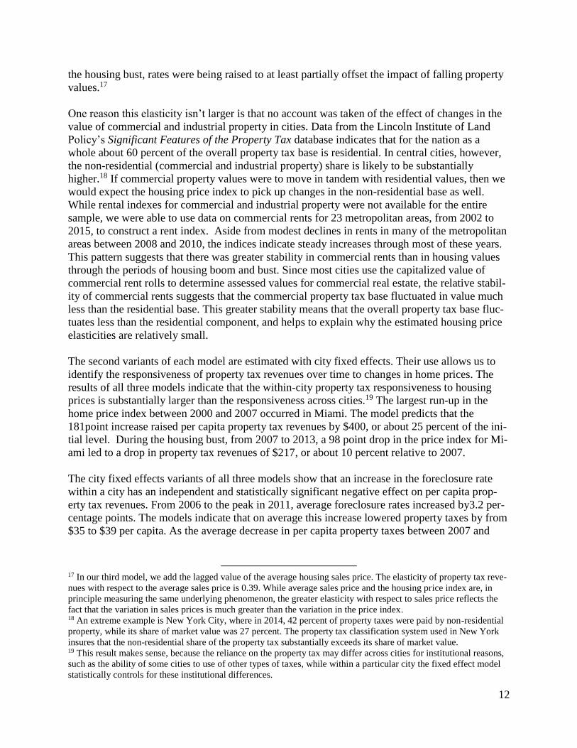
We can see from Figure 1 that city government spending in Baltimore, MD is almost three times

larger than city spending in Tampa, FL. However, when we account for the fact that many of the

local government services that city residents and businesses benefit from are provided by an

overlying school district and county government, total per capita spending in the two cities is al-

most identical.

To deal with the complexities of government organization, we developed the concept of a fis-

cally standardized city (FiSC). To construct each FiSC, we add up all the revenue collected

2

from or on behalf of central city residents and businesses, and similarly, add up on the local gov-

ernment spending flowing to central city residents, business, or visitors. This process involves

accounting for all revenue and spending of a central city municipal government and those por-

tions of revenue and spending by independent school districts, county governments, and special

districts that flow to central city residents.1 Although FiSCs have been constructed for 150 of the

nation’s largest central cities, in this paper we limit our sample to the 91 FiSCs for which we

have obtained detailed housing market data from CoreLogic.2

Pattern of Housing Stress in the 91 FiSCs

Although there was substantial variation across the country, the U.S. housing market over the

past 15 or so years was characterized by a rapid rise in housing prices through the first half of the

last decade, followed by a sharp fall in prices from about 2007 through 2012. Since then housing

prices have been rising, though in most places they remain below their peak in the last decade.3

1 For a detailed description of the methodology used in constructing the FiSC database see Howard Chernick, Adam

H. Langley, and Andrew Reschovsky. “Comparing Central City Finances Using Fiscally Standardized Cities,” Jour-

nal of Comparative Policy Analysis: Research and Practice 17, No. 4 (August 2015): 430-440. 2 The 150-city FiSC database is available at http://datatoolkits.lincolninst.edu/subcenters/fiscally-standardized-cit-

ies/. 3 The housing price data referenced in this sentence come from the housing price indices produced by the Federal

Housing Finance Agency.

$5,471

$1,903

$1,229

$1,553

$606

$1,379

$0

$1,000

$2,000

$3,000

$4,000

$5,000

$6,000

$7,000

Baltimore, MD Tampa, FL

Figure 1

Per Capita General Expenditures in the Baltimore and Tampa FiSCsby Type of Government, FY 2014

Special District

School

County

City

$6,077 $6,063

Type of Government

3

The boom and bust cycle of housing prices was accompanied by a very large rise in mortgage

delinquencies and housing foreclosures, with the foreclosure rate for the nation peaking in 2011.

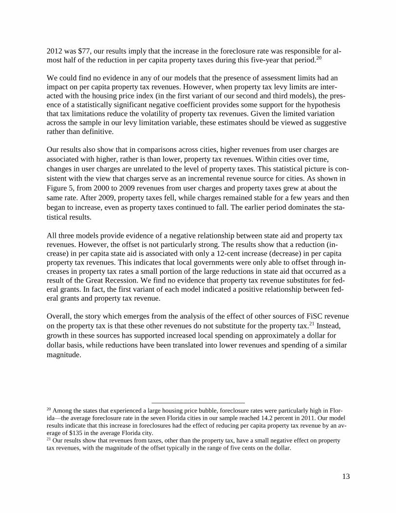
In Figure 2, we illustrate the average pattern of housing prices from 1997 through 2014 in the 91

central cities in our sample using data from the CoreLogic repeat-sales housing price index. The

figure also shows the housing price index for Las Vegas, a city that perhaps most clearly illus-

trates the boom-bust cycle in housing prices, and for Houston, a city that largely escaped both the

boom and the bust in housing prices. Prices in both Las Vegas and Houston closely tracked

prices in the average city from 1997 through 2003, when the patterns widely diverged. In both

cities, the 2003 housing price index was about 125; in the next three years it rose to 229 in Las

Vegas, while in Houston the index peaked in 2007 at 147. While prices in Houston declined

modestly, falling back to their 2004 levels in 2009, in Las Vegas, housing prices plummeted.

They reached their trough in 2011, at a price level equal to Las Vegas prices in 1997. Since

2012, housing prices in Houston have quite closely tracked prices in the average city. While

prices in Las Vegas are rising, they remain substantially below average.

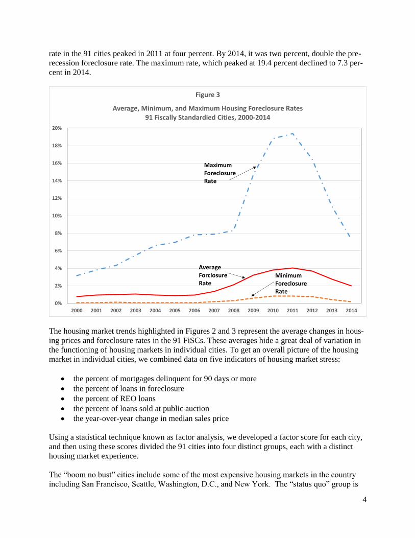
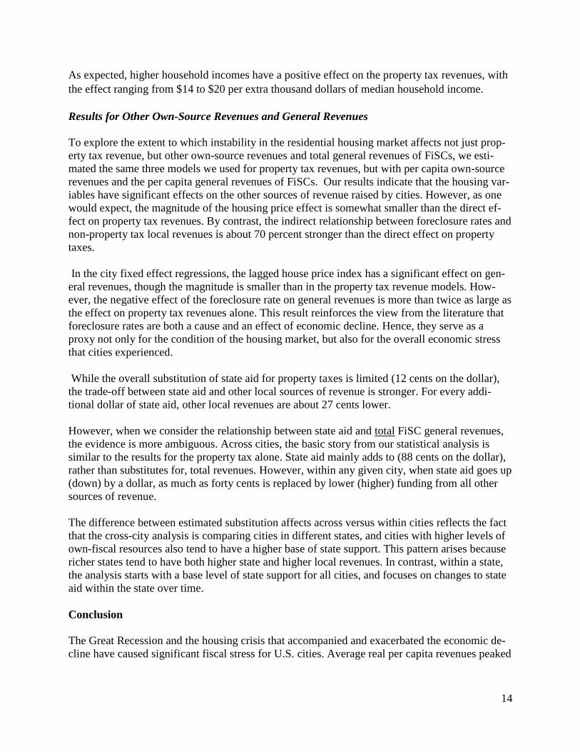
Figure 3 illustrates the pattern of foreclosure rates in the 91 central cities in our sample. Foreclo-

sure rates were calculated as the number of foreclosures divided by the number of mortgage

loans. The figure shows the average rate in the 91 cities and the range of foreclosure rates in each

year from 2000 through 2014. Through 2006 the average rate remained consistently below one

percent, although the maximum rate grew steadily from 3.2 percent to 7.8 percent. The average

80

90

100

110

120

130

140

150

160

170

180

190

200

210

220

230

1997 1998 1999 2000 2001 2002 2003 2004 2005 2006 2007 2008 2009 2010 2011 2012 2013 2014

Co

reLo

gic

Ho

usi

ng

Pri

ce In

dex

Figure 2

CoreLogic Housing Price Index, 1997-2014Average for 91 Central Cities, Las Vegas, and Houston

Housing Pricesin Las Vegas

Housing Pricesin Houston

Average Housing Pricesin 91 Central Cities

4

rate in the 91 cities peaked in 2011 at four percent. By 2014, it was two percent, double the pre-

recession foreclosure rate. The maximum rate, which peaked at 19.4 percent declined to 7.3 per-

cent in 2014.

The housing market trends highlighted in Figures 2 and 3 represent the average changes in hous-

ing prices and foreclosure rates in the 91 FiSCs. These averages hide a great deal of variation in

the functioning of housing markets in individual cities. To get an overall picture of the housing

market in individual cities, we combined data on five indicators of housing market stress:

the percent of mortgages delinquent for 90 days or more

the percent of loans in foreclosure

the percent of REO loans

the percent of loans sold at public auction

the year-over-year change in median sales price

Using a statistical technique known as factor analysis, we developed a factor score for each city,

and then using these scores divided the 91 cities into four distinct groups, each with a distinct

housing market experience.

The “boom no bust” cities include some of the most expensive housing markets in the country

including San Francisco, Seattle, Washington, D.C., and New York. The “status quo” group is

0%

2%

4%

6%

8%

10%

12%

14%

16%

18%

20%

2000 2001 2002 2003 2004 2005 2006 2007 2008 2009 2010 2011 2012 2013 2014

Figure 3

Average, Minimum, and Maximum Housing Foreclosure Rates91 Fiscally Standardied Cities, 2000-2014

AverageForclosureRate

Minimum ForeclosureRate

MaximumForeclosureRate

5

dominated by cities in Texas such as Dallas, Houston and Fort Worth, and cities such as Louis-

ville, Tulsa and Denver, where housing prices remained quite stable during the recessionary pe-

riod. Consistent with expectations, the largest proportion of cities, nearly one-third, are catego-

rized as “boom and bust” and include most of the cities in California and Florida, and of course

Las Vegas. Rust belt cities predominate in the “secular decline” group and include Detroit,

Cleveland and Cincinnati. These cities were characterized by very modest housing price in-

creases prior to the recession, and sharp declines during and immediately after the recession.

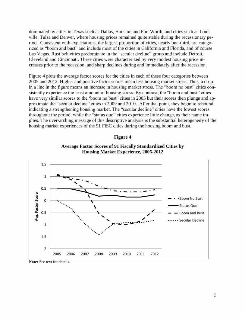
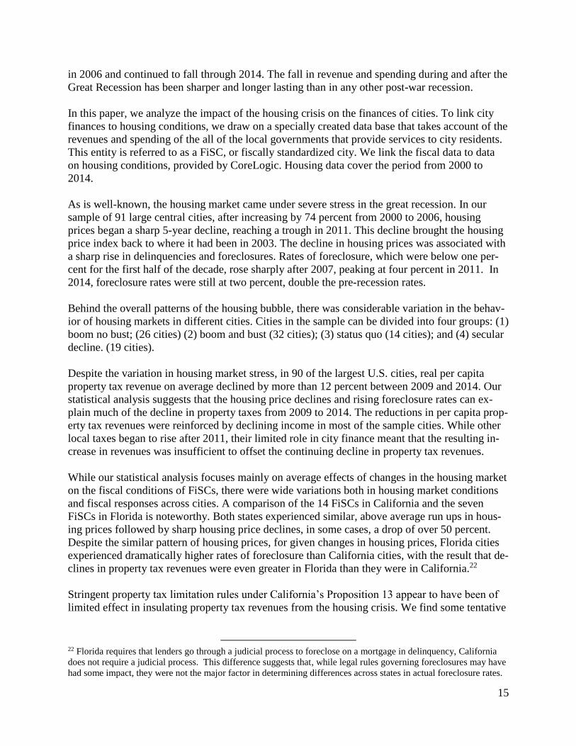
Figure 4 plots the average factor scores for the cities in each of these four categories between

2005 and 2012. Higher and positive factor scores mean less housing market stress. Thus, a drop

in a line in the figure means an increase in housing market stress. The “boom no bust” cities con-

sistently experience the least amount of housing stress. By contrast, the “boom and bust” cities

have very similar scores to the ‘boom no bust” cities in 2005 but their scores then plunge and ap-

proximate the “secular decline” cities in 2009 and 2010. After that point, they begin to rebound,

indicating a strengthening housing market. The “secular decline” cities have the lowest scores

throughout the period, while the “status quo” cities experience little change, as their name im-

plies. The over-arching message of this descriptive analysis is the substantial heterogeneity of the

housing market experiences of the 91 FiSC cities during the housing boom and bust.

Figure 4

Average Factor Scores of 91 Fiscally Standardized Cities by

Housing Market Experience, 2005-2012

Note: See text for details.

-2

-1.5

-1

-0.5

0

0.5

1

1.5

2005 2006 2007 2008 2009 2010 2011 2012

Avg

. Fa

cto

r Sc

ore

Boom No Bust

Status Quo

Boom and Bust

Secular Decline

6

Fiscal Conditions in the Nation’s Large Central Cities

The combination of the Great Recession, the sharp drop in the stock market, and the housing cri-

sis had a large impact on the financing of cities in the U.S. No economic downturn since the de-

pression of the 1930s has had as steep and as long lasting impact on city revenues and expendi-

tures. In FiSCs sample, average real per capita revenues peaked in 2007 and continued to fall

through 2014, the latest year for which these data are available.4 In 2014, average revenues were

8.3 percent lower than in 2007. Average per capita spending peaked in 2009, and by 2013, it had

fallen by 7.7 percent. In 2014, average spending began to rise, but only by 0.7 percent. Although

spending declines were not universal, real per capita spending in 2014 was still below 2009 lev-

els in 79 of the 90 fiscally standardized cities.

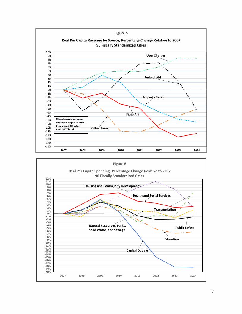
To provide a more detailed picture of recent fiscal developments in the 91 FiSCs, Figure 5 illus-

trates the changes in revenue by source in the average FiSC between 2007 and 2014. During this

period, state aid fell by about 11.5 percent and property taxes by 8.5 percent.5 Although revenues

from other taxes has increased since 2010, in 2014 they remained five percent below their pre-

recession (2007) level. After an initial decline, federal aid to FiSC governments rose above 2007

levels in 2010 and 2011, reflecting the increase in federal aid associated with the stimulus funds

distributed as part of the American Recovery and Reinvestment Act. Since then, real per capita

federal revenues have been declining. In 2014, revenue from federal grants in the average FiSC

was 5.3 percent below its level in 2007. The only revenues that rose in each year since 2007 were

from user charges. In 2014, user charges and fees were more than eight percent above their level

in 2007.6

As illustrated in Figure 6, after spending down available fund balances, the local government in

our FiSC sample began cutting public spending. Most categories of spending peaked in 2009,

and in 2014 remained below their 2007 (pre-recession) levels.7 In the average FiSC, per capita

real spending on education, by far the largest single category of local spending, was over six per-

cent lower than it was in 2007. The largest percentage reduction in spending was for capital out-

lays. In real per capita terms, they were 18.4 percent lower in 2014 than they had been in 2007.

Average spending on public safety was about one percent below its 2007 level, while spending

on natural resources, parks and recreation, sewage, and solid waste collection, housing and com-

munity development, and health and social services were all slightly higher in 2014 compared to

2007. Finally, transportation spending was about seven percent higher than it had been in 2007.

4 Because it has no state government, the District of Columbia is excluded from our FiSC sample in calculating the

statistics presented in this section. The District of Columbia is also excluded from the regression models discussed

in the next section. 5 In fiscal year 2007, revenue from the property tax accounted for about 24 percent of total revenue in the average

FiSC. State aid, which includes some federal grants to states that are passed through to local governments, made up

about 32 percent of total revenue. 6 In 2007, federal grants made up only 6.3 percent of general revenues of the average FiSC. User charges accounted

for 15 percent of revenue. 7 The capital outlay data in Figure 7 are total capital outlays for all expenditure functions, while the data for other

spending categories include only operating expenditures.

7

Federal Aid

State Aid

Property Taxes

Other Taxes

User Charges

-15%

-14%

-13%

-12%

-11%

-10%

-9%

-8%

-7%

-6%

-5%

-4%

-3%

-2%

-1%

0%

1%

2%

3%

4%

5%

6%

7%

8%

9%

10%

2007 2008 2009 2010 2011 2012 2013 2014

Figure 5

Real Per Capita Revenue by Source, Percentage Change Relative to 2007 90 Fiscally Standardized Cities

Miscellaneous revenuesdeclined sharply. In 2014they were 34% below their 2007 level.

-20%-19%-18%-17%-16%-15%-14%-13%-12%-11%-10%

-9%-8%-7%-6%-5%-4%-3%-2%-1%0%1%2%3%4%5%6%7%8%9%

10%11%12%

2007 2008 2009 2010 2011 2012 2013 2014

Figure 6

Real Per Capita Spending, Percentage Change Relative to 200790 Fiscally Standardized Cities

Health and Social Services

Capital Outlays

Public Safety

Transportation

Natural Resources, Parks,Solid Waste, and Sewage

Education

Housing and Community Development

8

The Impact of the Housing Market on the Revenue of FiSCs

To finance the wide array of public services provided to central city residents, local governments

require revenue streams that meet the needs of residents and businesses, that are buoyant enough

to support increased demands over time, and sufficiently stable to assure the provision of basic

services even during cyclical downturns.

Our primary research goal is to explore the various linkages between developments in the hous-

ing market and the revenues available to finance public services in the nation’s major central cit-

ies. In order to isolate and quantify the impact of various characteristics of the housing market on

the revenues of city governments, we estimate a set of multivariate statistical models. The mod-

els allow us to explore the various pathways through which developments in the housing market,

including the rise in foreclosure rates, influence the revenues available to city governments.

The most direct link between changes in the housing market and city government revenues is

through the property tax. Although the property tax is levied on both residential and business

property, over half of the property tax base in cities is composed of residential property. It would

thus be very surprising if the housing bubble of the past decade and the rapid rise in the number

of mortgage delinquencies and housing foreclosures did not have a direct effect on the property

tax base of central cities, and on their property tax revenues. Most of the limited research on the

linkages between the housing crisis and the fiscal condition of local governments has focused on

the relationship between changes in housing prices and changes in property tax revenues. This

literature consistently finds that changes in property tax revenues lags changes in housing prices

by at least a couple years.8 The only study to date of the links between foreclosures and property

tax revenues found that in the state of Georgia an increase in foreclosures led to a statistically

significant reduction in property tax revenues.9

For sales and income taxes, the relationship between changes in the economy and changes in tax

revenue is quite straightforward. Because sales and income tax rates are rarely changed, when

the sales of goods and services subject to taxation declines, sales tax revenues drop, and likewise,

if a recession results in lower incomes, income tax revenues decline. The relationship between

changes in housing prices and changes in property tax revenues is considerably more complex.

Changes in the market value of housing are not automatically reflected in changes in the property

tax base. Property taxes are based on the assessed value of housing, and reassessments generally

8 See Bryan F. Lutz, Raven Molloy, and Hui Shan, “The Housing Crisis and State and Local Government Tax Reve-

nue: Five Channels,” Regional Science and Urban Economics 41, No. 4 (July 2011): 306-319; James Alm, Robert

D. Buschman, and David L. Sjoquist, “Rethinking Local Government Reliance on the Property Tax,” Regional Sci-

ence and Urban Economics 41, Issue 4, (July 2011): 320-331; and Howard Chernick, Adam Langley, and Andrew

Reschovsky, “Predicting the Impact of the U.S. Housing Crisis and “Great Recession” on Central City Revenues,”

Publius: The Journal of Federalism 42, Issue 3 (Summer 2012): 467-493. 9 James Alm, Robert D. Buschman, and David L. Sjoquist. “Rethinking Local Government Reliance on the Property

Tax,” Regional Science and Urban Economics 41, Issue 4, (July 2011): 320-331.

9

occur on a regular cycle that is typically longer than a single year.10 After properties have been

reassessed, the new values serve as the basis for tax calculations in the following year. Once the

new property tax base (total assessed value) has been determined, local government officials set

a property tax rate sufficient to generate their desired level of property tax revenues (referred to

as their tax levy).11 This ability of local public officials to raise millage rates when property val-

ues decline, and lower rates when property values rise is one of the reasons why property tax rev-

enue has historically been more stable over a business cycle than sales and income tax revenues.

A second reason is that the property tax base, i.e. the market value of residential and non-resi-

dential property, is likely to be more stable than income or sales tax bases.

Because local government officials have control over their property tax rate, the property tax is

usually considered local governments’ residual source of revenue. This is the case because local

government officials have very limited control over their other major sources of revenue, namely

revenue from other taxes, from state intergovernmental transfers (state aid), and from federal

grants. In most states, local governments have limited, if any, discretion over both the tax base

and tax rates associated with local sales, excise, income, or payroll taxes. This implies that local

budgets, and property tax levies, are generally determined on the basis of expected revenues

from other taxes and intergovernmental transfers. For this reason, our models all include state

aid, federal aid, and revenue from other taxes.12

In many states the ability of local officials to determine property tax revenues is constrained by

voter-approved or state-imposed property tax limitations. More than 90 percent of the cities in

the FiSC sample are subject to some form of limitation, applying to tax rates, to the growth in tax

levies, or to the growth of assessed values of property. Property tax limitations are more likely to

apply to owner-occupied residential property than to rental or non-residential property.13

We expect that the overall effect of tax limitations will be to reduce the short-run responsiveness

of property tax revenues to changes in the value of the property tax base. However, the effect is

likely to vary depending on the degree of stringency of the limitation, and the magnitude of the

run up and subsequent decline in housing prices.14 In a period of rapid growth in housing values,

a tight limit may restrict governments’ ability to realize increased property tax levies from exist-

ing properties.

10 In some cities, for example New York, there are explicit caps on the annual rate of increase of assessed value.

These phase-in rules are likely to further lengthen the lag between changes in market values and changes in property

tax revenues. 11 Property tax rates are denominated in mills. A mill is equal to 1/10th of one percent (.001). 12 Local governments also raise revenue from user charges. The use of charges allows governments to fully or par-

tially finance government-provided services, such as recreational facilities, where the beneficiaries can be easily

identified. Thus, we expect user fee revenue to either be independent of or supplement property tax revenues. 13 In more than half of the cities there are provisions allowing voters to override limitations through the approval of

a referendum. 14 The best known of these limitations is California’s Proposition 13, which, unless a property is sold, limits the an-

nual increase in assessed value to the lesser of the inflation rate and 2 percent. Proposition 13 also set the maximum

allowable property tax rate at one percent. Given the rapid housing price appreciation that occurred in California in

recent decades, the assessed value of homes owned by many long-time property owners was substantially higher

than its current market value. Although housing prices fell dramatically in California after 2006, under Proposition

13 their assessed values continued to rise as long as the resulting assessed value remained below the, now dimin-

ished, market value.

10

We also hypothesize that the housing foreclosure rates in each city may have an independent ef-

fect on the property tax revenue of city governments. There may be a direct effect if the owners

of properties that are likely to be foreclosed stop paying property taxes. Also, residential and

non-residential property values may suffer in neighborhoods experiencing a rise in the number

and rate of foreclosure.

Changes in the level of household income are likely to influences property tax revenues via two

channels. First, the level of income affects the demand for public services, and hence the willing-

ness of residents to pay property taxes. Many studies have shown that the demand for local pub-

lic goods rises with income. Second, cities with higher levels of household income are generally

associated with both higher housing prices and higher commercial rents.15 Hence, higher median

incomes are associated with a higher value property tax bases. Both channels imply a positive

effect of income on property tax revenues.

Based on observed regional differences in property tax reliance, some of our models also in-

cludes regional indicator variables for each of the Census Bureau’s nine divisions (with New

England as the excluded division).

Data

Our empirical models are estimated using fiscal data from the Lincoln Institute’s Fiscally Stand-

ardized Cities database for the years 2000 through 2013 for 90 FiSCs for which we also have

housing market data provided by CoreLogic. All fiscal variables are measured in per capita infla-

tion-adjusted terms using 2013 dollars. In our analysis, we focus on two housing market

measures: a city-specific index of housing prices and the rate of housing foreclosures, measured

by the ratio of the number of foreclosures in a year, divided by the number of housing units with

mortgages. The housing price index is based on repeat sales within zip codes, with individual zip

code price changes aggregated up to a city-wide average. In one of our empirical specifications,

we supplement data on housing prices and foreclosures with data on the average sales price of

housing.

City-specific data on median household incomes comes from the 2000 decennial census and var-

ious 3-year American Community Surveys. Missing years are imputed based on annual income

changes in the state in which each city is located.

Existing literature suggests that the most binding form of property tax limitations are those that

limit the increase of property tax levies and those that limit the growth of the assessed values of

properties. We draw on a tax limitation typology developed by the Lincoln Institute of Land Pol-

icy, to distinguish between levy limitations and assessment limitations. Sixty five percent of the

15 Based on commercial rent data for a sub-sample of 24 or the largest metropolitan areas, the correlation between

the change in commercial rents between 2006 and 2014 and the change in household median income is 0.43, while

the correlation with median income per person equals 0.68.

11

sample have a limit on the increase in the tax levy, and a third of this group of cities also have a

limit on residential assessment growth.16

Empirical Strategy

In our attempt to explain the variation over time and across cities of per capita property tax reve-

nues, we estimate three models, each one with two variants. Each model is estimated for 90

FiSCs over the 11-year period from 2003 through 2013, a period that captures both the housing

bubble and the subsequent bust.

Each model includes the CoreLogic housing price index and a measure of the foreclosure rate.

Based on our previous research on the relationship between changes in housing values and

changes in property taxes, we lag the housing price index by three years. We tested for different

lags in the foreclosure effect, and found that a one period lag had the strongest fit statistically,

and produced the most plausible results.

Each model also contains per capita state aid and per capita federal aid, both lagged one year,

and per capita revenue from other taxes. All models include indicator variables for each year of

the sample. The first variant of each model contains regional indicator variables, reflecting the

Census division in which each city is located. The first variant of each model also includes an in-

dicator variable for each city in which residential property tax levies are subject to a state-im-

posed limitation. In the second variant of each model, the division codes are replaced by an indi-

vidual intercept term for each city. These are generally referred to as city fixed effects.

The only difference of the second model from the first model is the addition of a variable that in-

teracts the tax levy limitation variable with the lagged housing price index. The third model dif-

fers from the second by the addition of a variable measuring the average sales price of housing

lagged one year.

Property Tax Results

Confirming the results of previous literature, our three models all show a strong statistical rela-

tionship between housing prices (lagged three years) and the per capita property tax revenue of

FiSCs. To quantify the magnitude of statistical relationships, analysts often calculate elasticities,

which indicate the percentage in a given variable, in this case per capita property tax revenues,

for a one percent change in an explanatory variable, in this case, the housing price index. Evalu-

ated at the average value of the housing price index, we calculated an elasticity of the property

tax with respect to the housing price index of about 0.17. This elasticity indicates that on average

a 10 percent increase (decrease) in housing prices is associated with a 1.7 percent increase (de-

crease) in property tax revenues. This result implies that during the housing boom, city govern-

ments were lowering property tax rates in response to rising assessed property values, and during

16 Our measures of property tax limitations were compiled from information in the Significant Features of the Prop-

erty Tax online database. All of the limitations were enacted prior to 2000, and have remained unchanged during the

period of time covered by our analysis.

12

the housing bust, rates were being raised to at least partially offset the impact of falling property

values.17

One reason this elasticity isn’t larger is that no account was taken of the effect of changes in the

value of commercial and industrial property in cities. Data from the Lincoln Institute of Land

Policy’s Significant Features of the Property Tax database indicates that for the nation as a

whole about 60 percent of the overall property tax base is residential. In central cities, however,

the non-residential (commercial and industrial property) share is likely to be substantially

higher.18 If commercial property values were to move in tandem with residential values, then we

would expect the housing price index to pick up changes in the non-residential base as well.

While rental indexes for commercial and industrial property were not available for the entire

sample, we were able to use data on commercial rents for 23 metropolitan areas, from 2002 to

2015, to construct a rent index. Aside from modest declines in rents in many of the metropolitan

areas between 2008 and 2010, the indices indicate steady increases through most of these years.

This pattern suggests that there was greater stability in commercial rents than in housing values

through the periods of housing boom and bust. Since most cities use the capitalized value of

commercial rent rolls to determine assessed values for commercial real estate, the relative stabil-

ity of commercial rents suggests that the commercial property tax base fluctuated in value much

less than the residential base. This greater stability means that the overall property tax base fluc-

tuates less than the residential component, and helps to explain why the estimated housing price

elasticities are relatively small.

The second variants of each model are estimated with city fixed effects. Their use allows us to

identify the responsiveness of property tax revenues over time to changes in home prices. The

results of all three models indicate that the within-city property tax responsiveness to housing

prices is substantially larger than the responsiveness across cities.19 The largest run-up in the

home price index between 2000 and 2007 occurred in Miami. The model predicts that the

181point increase raised per capita property tax revenues by $400, or about 25 percent of the ini-

tial level. During the housing bust, from 2007 to 2013, a 98 point drop in the price index for Mi-

ami led to a drop in property tax revenues of $217, or about 10 percent relative to 2007.

The city fixed effects variants of all three models show that an increase in the foreclosure rate

within a city has an independent and statistically significant negative effect on per capita prop-

erty tax revenues. From 2006 to the peak in 2011, average foreclosure rates increased by3.2 per-

centage points. The models indicate that on average this increase lowered property taxes by from

$35 to $39 per capita. As the average decrease in per capita property taxes between 2007 and

17 In our third model, we add the lagged value of the average housing sales price. The elasticity of property tax reve-

nues with respect to the average sales price is 0.39. While average sales price and the housing price index are, in

principle measuring the same underlying phenomenon, the greater elasticity with respect to sales price reflects the

fact that the variation in sales prices is much greater than the variation in the price index. 18 An extreme example is New York City, where in 2014, 42 percent of property taxes were paid by non-residential

property, while its share of market value was 27 percent. The property tax classification system used in New York

insures that the non-residential share of the property tax substantially exceeds its share of market value. 19 This result makes sense, because the reliance on the property tax may differ across cities for institutional reasons,

such as the ability of some cities to use of other types of taxes, while within a particular city the fixed effect model

statistically controls for these institutional differences.

13

2012 was $77, our results imply that the increase in the foreclosure rate was responsible for al-

most half of the reduction in per capita property taxes during this five-year that period.20

We could find no evidence in any of our models that the presence of assessment limits had an

impact on per capita property tax revenues. However, when property tax levy limits are inter-

acted with the housing price index (in the first variant of our second and third models), the pres-

ence of a statistically significant negative coefficient provides some support for the hypothesis

that tax limitations reduce the volatility of property tax revenues. Given the limited variation

across the sample in our levy limitation variable, these estimates should be viewed as suggestive

rather than definitive.

Our results also show that in comparisons across cities, higher revenues from user charges are

associated with higher, rather is than lower, property tax revenues. Within cities over time,

changes in user charges are unrelated to the level of property taxes. This statistical picture is con-

sistent with the view that charges serve as an incremental revenue source for cities. As shown in

Figure 5, from 2000 to 2009 revenues from user charges and property taxes grew at about the

same rate. After 2009, property taxes fell, while charges remained stable for a few years and then

began to increase, even as property taxes continued to fall. The earlier period dominates the sta-

tistical results.

All three models provide evidence of a negative relationship between state aid and property tax

revenues. However, the offset is not particularly strong. The results show that a reduction (in-

crease) in per capita state aid is associated with only a 12-cent increase (decrease) in per capita

property tax revenues. This indicates that local governments were only able to offset through in-

creases in property tax rates a small portion of the large reductions in state aid that occurred as a

result of the Great Recession. We find no evidence that property tax revenue substitutes for fed-

eral grants. In fact, the first variant of each model indicated a positive relationship between fed-

eral grants and property tax revenue.

Overall, the story which emerges from the analysis of the effect of other sources of FiSC revenue

on the property tax is that these other revenues do not substitute for the property tax.21 Instead,

growth in these sources has supported increased local spending on approximately a dollar for

dollar basis, while reductions have been translated into lower revenues and spending of a similar

magnitude.

20 Among the states that experienced a large housing price bubble, foreclosure rates were particularly high in Flor-

ida—the average foreclosure rate in the seven Florida cities in our sample reached 14.2 percent in 2011. Our model

results indicate that this increase in foreclosures had the effect of reducing per capita property tax revenue by an av-

erage of $135 in the average Florida city. 21 Our results show that revenues from taxes, other than the property tax, have a small negative effect on property

tax revenues, with the magnitude of the offset typically in the range of five cents on the dollar.

14

As expected, higher household incomes have a positive effect on the property tax revenues, with

the effect ranging from $14 to $20 per extra thousand dollars of median household income.

Results for Other Own-Source Revenues and General Revenues

To explore the extent to which instability in the residential housing market affects not just prop-

erty tax revenue, but other own-source revenues and total general revenues of FiSCs, we esti-

mated the same three models we used for property tax revenues, but with per capita own-source

revenues and the per capita general revenues of FiSCs. Our results indicate that the housing var-

iables have significant effects on the other sources of revenue raised by cities. However, as one

would expect, the magnitude of the housing price effect is somewhat smaller than the direct ef-

fect on property tax revenues. By contrast, the indirect relationship between foreclosure rates and

non-property tax local revenues is about 70 percent stronger than the direct effect on property

taxes.

In the city fixed effect regressions, the lagged house price index has a significant effect on gen-

eral revenues, though the magnitude is smaller than in the property tax revenue models. How-

ever, the negative effect of the foreclosure rate on general revenues is more than twice as large as

the effect on property tax revenues alone. This result reinforces the view from the literature that

foreclosure rates are both a cause and an effect of economic decline. Hence, they serve as a

proxy not only for the condition of the housing market, but also for the overall economic stress

that cities experienced.

While the overall substitution of state aid for property taxes is limited (12 cents on the dollar),

the trade-off between state aid and other local sources of revenue is stronger. For every addi-

tional dollar of state aid, other local revenues are about 27 cents lower.

However, when we consider the relationship between state aid and total FiSC general revenues,

the evidence is more ambiguous. Across cities, the basic story from our statistical analysis is

similar to the results for the property tax alone. State aid mainly adds to (88 cents on the dollar),

rather than substitutes for, total revenues. However, within any given city, when state aid goes up

(down) by a dollar, as much as forty cents is replaced by lower (higher) funding from all other

sources of revenue.

The difference between estimated substitution affects across versus within cities reflects the fact

that the cross-city analysis is comparing cities in different states, and cities with higher levels of

own-fiscal resources also tend to have a higher base of state support. This pattern arises because

richer states tend to have both higher state and higher local revenues. In contrast, within a state,

the analysis starts with a base level of state support for all cities, and focuses on changes to state

aid within the state over time.

Conclusion

The Great Recession and the housing crisis that accompanied and exacerbated the economic de-

cline have caused significant fiscal stress for U.S. cities. Average real per capita revenues peaked

15

in 2006 and continued to fall through 2014. The fall in revenue and spending during and after the

Great Recession has been sharper and longer lasting than in any other post-war recession.

In this paper, we analyze the impact of the housing crisis on the finances of cities. To link city

finances to housing conditions, we draw on a specially created data base that takes account of the

revenues and spending of the all of the local governments that provide services to city residents.

This entity is referred to as a FiSC, or fiscally standardized city. We link the fiscal data to data

on housing conditions, provided by CoreLogic. Housing data cover the period from 2000 to

2014.

As is well-known, the housing market came under severe stress in the great recession. In our

sample of 91 large central cities, after increasing by 74 percent from 2000 to 2006, housing

prices began a sharp 5-year decline, reaching a trough in 2011. This decline brought the housing

price index back to where it had been in 2003. The decline in housing prices was associated with

a sharp rise in delinquencies and foreclosures. Rates of foreclosure, which were below one per-

cent for the first half of the decade, rose sharply after 2007, peaking at four percent in 2011. In

2014, foreclosure rates were still at two percent, double the pre-recession rates.

Behind the overall patterns of the housing bubble, there was considerable variation in the behav-

ior of housing markets in different cities. Cities in the sample can be divided into four groups: (1)

boom no bust; (26 cities) (2) boom and bust (32 cities); (3) status quo (14 cities); and (4) secular

decline. (19 cities).

Despite the variation in housing market stress, in 90 of the largest U.S. cities, real per capita

property tax revenue on average declined by more than 12 percent between 2009 and 2014. Our

statistical analysis suggests that the housing price declines and rising foreclosure rates can ex-

plain much of the decline in property taxes from 2009 to 2014. The reductions in per capita prop-

erty tax revenues were reinforced by declining income in most of the sample cities. While other

local taxes began to rise after 2011, their limited role in city finance meant that the resulting in-

crease in revenues was insufficient to offset the continuing decline in property tax revenues.

While our statistical analysis focuses mainly on average effects of changes in the housing market

on the fiscal conditions of FiSCs, there were wide variations both in housing market conditions

and fiscal responses across cities. A comparison of the 14 FiSCs in California and the seven

FiSCs in Florida is noteworthy. Both states experienced similar, above average run ups in hous-

ing prices followed by sharp housing price declines, in some cases, a drop of over 50 percent.

Despite the similar pattern of housing prices, for given changes in housing prices, Florida cities

experienced dramatically higher rates of foreclosure than California cities, with the result that de-

clines in property tax revenues were even greater in Florida than they were in California.22

Stringent property tax limitation rules under California’s Proposition 13 appear to have been of

limited effect in insulating property tax revenues from the housing crisis. We find some tentative

22 Florida requires that lenders go through a judicial process to foreclose on a mortgage in delinquency, California

does not require a judicial process. This difference suggests that, while legal rules governing foreclosures may have

had some impact, they were not the major factor in determining differences across states in actual foreclosure rates.

16

evidence, however, that in cities with levy limitations the effect of changes in housing prices on

property tax levels was somewhat smaller than in cities that did not have levy limitations.

The decline in city revenues since the Great Recession is greater than any such decline, at least

since 1977. A number of analyses have pointed to the crucial role of housing in exacerbating the

effect of the recession and delaying the recovery. From a macroeconomic perspective, the sharp

decline and very slow recovery of the state and local sector served as an important contributor to

the severity of the recession, and one of the main impediments to a robust economic recovery.

Our analysis of the effects of the housing bubble on city revenues from all sources, including

state aid, represents an important channel through which stress in housing markets affects re-

gional economies as well as the overall macro economy.

Policy Implications

The principle lesson from our analysis is that real estate bubbles carry with them significant fis-

cal risks for cities. True bubbles are invariably followed by busts, and busts lead to significant

declines in local government revenues. If the busts are associated with an overall decline in a

state’s economy, the losses in local revenue are likely to be reinforced by declining state aid to

its local governments. Because cities must balance their budgets from year to year, these declines

inevitably mean that spending must be cut. The typical city fiscal response to the Great Reces-

sion and the housing bust was to implement substantial reductions in spending, with the largest

cuts occurring in capital outlays and in operating expenditures for elementary and secondary ed-

ucation.

We conclude with three policy recommendations that flow from our analysis:

The evidence shows that most cities increase revenues when housing prices rise. These

revenue increases generally occur despite the presence of property tax limitations. As ris-

ing housing prices may foreshadow a coming housing price drop, local governments

should exploit a period of rising housing prices by preparing for the fiscal consequences

of a future drop in prices. This could be done by increasing fund balances (rainy day

funds), or by utilizing additional revenues to pre-fund future capital infrastructure pro-

jects.

States should pursue policies to try to minimize foreclosures during future housing mar-

ket declines.

Because the fiscal effects of housing busts play out over a multiyear time horizon, offset-

ting increases in federal aid should be structured to provide increased fiscal assistance

over multiyear time periods.