The Effect of Taxes and Transfers on Income and Poverty in ...

U S C E N S U S B U R E A UHelping You Make Informed Decisions

U.S.Department of CommerceEconomics and Statistics Administration

U.S. CENSUS BUREAU

The Effect of Taxes and Transferson Income and Poverty in theUnited States: 2005Consumer Income

Issued March 2007

CurrentPopulationReports

P60-232

INTRODUCTION losses, and work expenses) varies at ahousehold level.

This report examines how income distri-butions change when the definition of This report presents medians that illus-income is varied to reflect the inclusion trate the aggregate impact of all of theseor exclusion of different components. programs and transfers on income distri-The measure of household income bution. Money income is compared withreported in the publication Income, three additional income definitions: mar-Poverty, and Health Insurance Coverage ket income, post-social insurancein the United States: 2005 (P60-231) uses income, and disposable income. Thesethe pretax, money income concept. measures are presented to illustrate vari-Money income in this instance includes ous dimensions of economic well-beingcash income before taxes are paid. and the impact of taxes and transfers.

The text box called “Definitions ofThe government provides resources to

Income” details the components of thesehouseholds through cash and noncash

income definitions.1

transfer programs. These programs maybe open to all or limited to those with While the income definitions presented inincomes below set amounts. Holding this report resemble the income meas-other income components constant, urements recommended by the Canberratransfers from the Social Security Group (an international group of house-Administration, Veterans Administration, hold income experts convened under theand state governments increase house- auspices of the United Nations Statisticshold income. Payroll, state, and federal Division), the definitions differ, due totax liabilities reduce household income. both the lack of certain elements in theCertain tax credits, such as the Earned survey data and ongoing developmentalIncome Tax Credit and the Additional efforts.2 This report does not presentChild Tax Credit, are refundable and may international comparisons.increase household income.

This report also includes imputed 1 A list of variables included in each definition is

resource measures not directly related to available at <www.census.gov/hhes/www/income/definitions.html>.

government programs. Imputed realized 2 Money income in this report is similar to thecapital gains and rental income on Canberra Total Income concept. Disposable income is

similar to the Canberra Adjusted Disposable Incomeowner-occupied homes increase house- concept. Canberra suggested adding some compo-hold income; imputed realized capital nents, such as the value of home production, which are

losses and work expenses decrease not incorporated into the income definitions reportedhere. Another difference is that the Canberra Report

household income. The net impact of does not include realized capital gains and losses,

positive transfers (government pro- which are imputed for use in this report. For furtherexplanations about the Canberra Group’s recommenda-

grams, realized capital gains, and tions, see <www.lisproject.org/links/canberra

imputed rent estimates) and negative /finalreport.pdf>. Development efforts includeimprovements to the modeling used to impute flows

transfers (tax liabilities, realized capital from capital gains, imputed rent, and noncash benefits.

This report presents alternative measures of incomethat include estimates of taxes and values of vari-ous noncash benefits for calendar years 2004 and2005. These measures were derived from informa-tion collected in the 2005 and 2006 Annual Socialand Economic Supplements (ASEC) to the CurrentPopulation Survey (CPS). The following terms areused to describe the four measures of income usedin this report:

Money Income: Includes all cash income receivedby individuals who are 15 years or older. It consistsof income as reported, before deductions for taxesand other expenses. It does not include realizedcapital gains or lump-sum payments that may bedisbursed from insurance companies, workers’ com-pensation, or pension plans.

Market Income: Includes money income asdescribed above and deducts government cash trans-fers. Government cash transfers are social security;supplemental security income (SSI); public assistance(including Temporary Assistance for Needy Families[TANF]); unemployment compensation; workers’ com-pensation; veterans’ payments; and survivor, pension,and disability benefits from certain sources.3 Thisdefinition also includes imputed net realized capitalgains and imputed rental income (also called returnon home equity) and subtracts imputed workexpenses excluding child care.4

Post-Social Insurance Income: Includes moneyincome, imputed net realized capital gains, andimputed rental income; subtracts imputed workexpenses as in market income; and also deductsgovernment means-tested cash transfers. Theseinclude SSI, public assistance, and government paidmeans-tested veterans’ payments. Post-social insur-ance income differs from market income by addingback non-means-tested government transfers, mostnotably social security.5

Disposable Income: Includes money income,imputed net realized capital gains, and imputedrental income; and subtracts imputed workexpenses. Disposable income also deducts federalpayroll taxes, federal and state income taxes, andproperty taxes for owner-occupied homes.6 Thevalue of noncash transfers is added, including foodstamps, public or subsidized housing, and free orreduced-price school lunches.7

DEFINITIONS OF INCOME

3 Government paid survivor, pension, and disability benefitsinclude those paid by workers’ compensation, U.S. RailroadRetirement, Black Lung Benefits, and State Temporary Sickness.

4 Capital gains and losses are imputed using a statistical matchto the 2001 Statistics of Income public use file from the InternalRevenue Service as part of the CPS ASEC tax model. For modeledtax filers, the imputed amounts are added to money income andare included as taxable income. Imputed rental income reflects theincome homeowners would receive if they rented out their home;this value is added to money income to put homeowners andrenters on a more equal footing. The return on home equityimputed for the CPS ASEC is an approximation of this income flowcomputed by applying a rate of return to imputed home equity.The American Housing Survey (AHS) provides the home and landvalues and mortgage debt used to compute home equity. The cur-rent year’s return on municipal bonds is used as the rate of return.The 2006 ASEC uses 2003 National AHS data. Previous years used

home equity based on 1995 National AHS data. This modelingimprovement was repeated for the 2005 ASEC to make valid year-to-year comparisons in Table A-1. Work expenses are imputedfrom the Survey of Income and Program Participation (SIPP) 2001Panel. The Census Bureau is considering changes to its child-careexpenses imputation procedures and is deferring their inclusion inthe report until either the current method can be validated or animproved method can be found.

5 Non-means-tested government transfers include unemploymentcompensation, workers’ compensation, social security, and the sur-vivor, pension, and disability benefits described in footnote 18.

6 Property taxes are imputed from the 2003 National AHS.7 The reported value of food stamps is used; the value of hous-

ing subsidies is modeled using the 1985 National AHS; and thevalue of school lunches is modeled using parameters from theFood and Nutrition Service of the U.S. Department of Agriculture.

2 U.S. Census Bureau

Using households as the units ofanalysis for income and using peo-ple as the units of analysis forpoverty, this report primarily pres-ents data for income year 2005using information collected in the2006 Annual Social and EconomicSupplement (ASEC) to the CurrentPopulation Survey (CPS). The CPSASEC is augmented with data fromthe Internal Revenue Service, theU.S. Department of Agriculture, andthe U.S. Department of Housing andUrban Development to compute thethree income definitions. Thisreport examines interdefinition dif-ferences and intradefinition compar-isons; it then examines changesfrom 2004 to 2005.

In the 1990s, the NationalAcademies of Science (NAS) con-vened a panel to review howpoverty is measured (Citro andMichael, 1995). The panelasserted that any change in theincome definition used to deter-mine how much a person or a fam-ily needs to meet the basic neces-sities of life should beaccompanied by a consistentadjustment of the measure of basicnecessities (Recommendation 41.1,P. 10.) Further, that group ofresearchers believed it is necessary

to update the thresholds used todefine poverty, which were devel-oped in the 1960s, to fullyrepresent a person’s or a family’schanging needs. Although the U.S.Census Bureau has produced sev-eral reports based on the NASpanel’s recommendations, thisreport does not address thesepoverty threshold issues. (Short,1999, and Dalaker, 2003, use theNAS recommendations.) Ratherthan propose a revised measure ofpoverty, this report examines theeffects of changing the resourcedefinitions.8 Different income defi-nitions are compared to a set ofthresholds that vary by the sizeand the composition of the family,but the same thresholds are usedregardless of the income defini-tion. The thresholds are based onthe four-person family thresholddesigned by Mollie Orshansky inthe 1960s.

U.S. Census Bureau 3

8 Alternative poverty estimates based onthe NAS recommendations for 2005 areavailable at <www.census.gov/hhes/www/povmeas/nas.html>. The main differencesbetween the measures presented in thisreport and the NAS measures are the inclu-sion of medical care and child-care expensesin the NAS estimates, the inclusion ofimputed rent in the estimates in this report,and the use of different thresholds.

Household Income

The effects of government taxesand transfers on 2005 medianhousehold income are shown inTable 1 by comparing the traditionalmoney income concept with thethree alternative definitions: marketincome, post-social insuranceincome, and disposable income.

Market income representsresources available to people andfamilies based on labor and capitalmarket activities and does notinclude income from governmentsources including social securityand public assistance.9 It includesimputed rental income for owner-occupied housing and imputedrealized capital gains and losses.Work expenses, excluding child-care costs, are also deducted toarrive at market income.10 Thenumber of households with netdeductions exceeds the number ofhouseholds with net additionsfrom market sources. The result ismedian household market incomethat is lower than under the moneyincome definition. Median house-hold market income was $43,701in 2005, or 5.7 percent lower thanmedian household money income,$46,326. Market income can serveas a reference point to evaluate theimpact of government transfersand the imputed return on homeequity across the income distribu-tion and the effect of imputed real-ized capital gains at the high endof the income distribution.

9 Refer to text box “Definitions ofIncome” for a listing of all government cashtransfers that are deducted from moneyincome.

10 The Census Bureau is consideringchanges to its child-care expenses imputa-tion procedures and is deferring their inclu-sion in the report until either the currentmethod can be validated or an improvedmethod can be found.

Table 1.Median Income of Households by Income Definition: 2005

Percent Percentdifference difference

Definition Median from from moneyincome previous income

(dollars) definition definition

Money income . . . . . . . . . . . . . . . . . . . . . . . . . . . 46,326 (X) (X)Market income . . . . . . . . . . . . . . . . . . . . . . . . . . 43,701 –5.7 –5.7Post-social insurance income . . . . . . . . . . . . . 47,975 9.8 3.6Disposable income . . . . . . . . . . . . . . . . . . . . . . . 40,843 –14.9 –11.8

(X) Not applicable.Source: U.S. Census Bureau, Current Population Survey, 2006 Annual Social and Economic

Supplement.

Post-social insurance income isdefined as market income plusnon-means-tested governmentcash transfers, such as social secu-rity, unemployment compensation,and workers’ compensation.Households with income from atleast one of these sources havehigher post-social insuranceincome than market income. Thus,at $47,975 in 2005, median house-hold post-social insurance incomewas higher than median householdmarket income.

Disposable income has the lowestmedian income of all the defini-tions and represents the netincome households have availableto meet living expenses.Disposable income includes allresources in post-social insuranceincome and adds the value of

noncash transfers such as foodstamps, public or subsidized hous-ing, and school lunches, alongwith means-tested cash transfers,while deducting property taxes,payroll taxes, and state and federalincome taxes.11 The net result ofthese additions and deductionslowered median household incomeby 14.9 percent from the post-social insurance income definition.At $40,843, the median householddisposable income estimate is 11.8 percent lower than incomeunder the money income defini-tion, $46,326.

Table 2 uses median money incomeas the base to gauge the effects ofthe other income definitions on


11 More information on how taxes aremodeled in the CPS ASEC can be found inO’Hara, 2004.

subgroups of households. It showshow the inclusion and exclusion ofincome components under the vari-ous definitions affects the income ofvarious demographic groups. Forhouseholds with a female house-holder with no husband present, themarket income definition results in amedian that is 88.4 percent of theirmedian household money income.12

For married-couple households,median market income composes99.2 percent of their median money

12 The householder is the person (or oneof the people) in whose name the home isowned or rented and the person to whomthe relationship of other household membersis recorded. If a married couple jointly ownsthe home, either the husband or the wifemay be listed as the householder. Since onlyone person in each household is designatedas the householder, the number of house-holders is equal to the number of house-holds. This report uses the characteristics ofthe householder to describe the household.

Table 2.Index of Median Household Income by Selected Characteristic and Income Definition:2005

Characteristic

Moneyincome

Marketincome

Post-social insuranceincome

Disposableincome

Median(dollars)

Percent ofmoneyincome

Median(dollars)


Median(dollars)


Median(dollars)


All households . . . . . . . . . . 46,326 100.0 43,701 94.3 47,975 103.6 40,843 88.2

Type of Household

Family households . . . . . . . . . . . . . . . . 57,278 100.0 55,650 97.2 59,731 104.3 50,707 88.5Married-couple . . . . . . . . . . . . . . . . . . 66,067 100.0 65,564 99.2 69,349 105.0 57,786 87.5Female householder, no husband

present . . . . . . . . . . . . . . . . . . . . . . . 30,650 100.0 27,107 88.4 30,419 99.2 29,464 96.1Nonfamily households . . . . . . . . . . . . . 27,326 100.0 24,712 90.4 29,395 107.6 25,283 92.5

Race1 and Hispanic Origin

White . . . . . . . . . . . . . . . . . . . . . . . . . . . . 48,554 100.0 46,153 95.1 50,482 104.0 42,883 88.3White, not Hispanic . . . . . . . . . . . . . 50,784 100.0 48,513 95.5 53,142 104.6 44,599 87.8

Black . . . . . . . . . . . . . . . . . . . . . . . . . . . . 30,858 100.0 27,370 88.7 30,713 99.5 28,416 92.1Asian . . . . . . . . . . . . . . . . . . . . . . . . . . . . 61,094 100.0 61,505 100.7 64,362 105.3 53,051 86.8

Hispanic origin (any race) . . . . . . . . . . 35,967 100.0 33,730 93.8 35,744 99.4 32,769 91.1

Work Experience of Householder

Worked . . . . . . . . . . . . . . . . . . . . . . . . . . 57,802 100.0 57,510 99.5 59,326 102.6 48,561 84.0Worked full-time, year-round . . . . . 63,610 100.0 64,232 101.0 65,537 103.0 52,711 82.9

Did not work . . . . . . . . . . . . . . . . . . . . . . 23,801 100.0 13,973 58.7 27,421 115.2 26,478 111.2

1 Federal surveys now give respondents the option of reporting more than one race. Therefore, two basic ways of defining a race group are possible. Agroup such as Asian may be defined as those who reported Asian and no other race (the race-alone or single-race concept) or as those who reported Asianregardless of whether they also reported another race (the race-alone-or-in-combination concept). This table shows data using the first approach (race alone).The use of the single-race population does not imply that it is the preferred method of presenting or analyzing data. The Census Bureau uses a variety ofapproaches. Information on people who reported more than one race, such as White and Asian or Asian and Black or African American, is available fromCensus 2000 through American FactFinder. About 2.6 percent of people reported more than one race in Census 2000.

Source: U.S. Census Bureau, Current Population Survey, 2006 Annual Social and Economic Supplement.

income. Households with a femalehouseholder with no husband pres-ent typically have incomes lowenough to be affected by the deduc-tion of work expenses and govern-ment transfers in the market incomedefinition. The post-social insuranceincome definition brings the femalehouseholder with no husband pres-ent index value nearer to the moneyincome base by adding back non-means-tested government transfers.Median disposable householdincome for female householderswith no husband present is 96.1percent of median money income.By incorporating noncash transfers(such as food stamps, housing sub-sidies, and school lunches), means-tested cash transfers, and taxes, thisdefinition affects female household-ers with no husband present morethan other household types.Noncash transfers and tax credits,such as the Earned Income TaxCredit, add resources to low-incomehouseholds, but subtractions forwork expenses and payroll taxesprevent the median disposableincome from equaling the full basevalue of median money income.

Asian households have the highestmedian money income ($61,094)among the race groups shown inTable 2.13 While median marketincome is lower than median


13 Federal surveys now give respondentsthe option of reporting more than one race.Therefore, two basic ways of defining a racegroup are possible. A group such as Asianmay be defined as those who reported Asianand no other race (the race-alone or single-race concept) or as those who reported Asianregardless of whether they also reportedanother race (the race-alone-or-in-combinationconcept). The body of this report (text, fig-ures, and tables) shows data using the firstapproach (race alone). Use of the single-racepopulation does not imply that it is the pre-ferred method of presenting or analyzingdata. The Census Bureau uses a variety ofapproaches. The CPS does not use separatepopulation controls for weighting the Asiansample to national totals.

In this report, the term “non-HispanicWhite” refers to people who are not Hispanicand who reported White and no other race.The Census Bureau uses non-Hispanic Whitesas the comparison group for other racegroups and Hispanics.

money income for all households,Asian households have highermedian household market incomethan median money income (100.7percent of median money income).Asian households have one of thehighest relative percentages ofmedian post-social insuranceincome to money income, at 105.3percent, and one of the lowest rela-tive percentages of median dispos-able income to money income, at86.8 percent.14 These figures indi-cate that Asian households areaffected less by the subtraction ofgovernment transfers and areaffected more by the deduction ofmodeled taxes or the inclusion ofimputed realized capital gains andnet rent.

Among race groups and Hispanics,median money income is lowestfor Black households and Hispanichouseholds ($30,858 and $35,967,respectively).15 In addition, Blackhouseholds had the lowest ratio,by race and Hispanic origin, ofmedian market income to medianmoney income when governmentcash transfers and work expensesare deducted (88.7 percent).Conversely, Black households andHispanic households have thehighest ratios of median dispos-able income to money income.Black households have median dis-posable income that is 92.1 per-cent of the group’s median moneyincome, and Hispanic householdshave median disposable incomethat is 91.1 percent of their

14 Not statistically different from Whiteand White alone, not Hispanic.

15 Because Hispanics may be any race,data in this report for Hispanics overlap withdata for racial groups. Data users shouldexercise caution when interpreting aggregateresults for the Hispanic population or for racegroups because these populations consist ofmany distinct groups that differ in socioeco-nomic characteristics, culture, and recency ofimmigration. Data were first collected forHispanics in 1972 and for Asians and PacificIslanders in 1987. For further information, see<www.bls.census.gov/cps/ads/adsmain.htm>.

median money income.16 This sug-gests that Black and Hispanichouseholds (those with lowermedian money income) are beingpositively affected by governmentcash and noncash transfers suchas public assistance, includingTemporary Assistance for NeedyFamilies (TANF), public or subsi-dized housing, and food stamps.

Households with a householderwho did not work have lowermedian money income ($23,801)than households with a workinghouseholder ($57,802). Amongthe work experience comparisonsin Table 2, the households with ahouseholder who did not work dis-play the largest difference betweenmoney income and market income,with a ratio of 58.7 percent.Households with a nonworkinghouseholder include a high per-centage of nonworking elderly, dis-abled, or other low-income house-holders. The median householdmarket income of the elderly isaffected by the deduction of socialsecurity, government-paid veter-ans’ payments, survivor benefits,and disability benefits. Low-income households are affected bythe deduction of governmentmeans-tested cash transfers suchas supplemental security income(SSI) and public assistance in themarket and post-social insurancedefinitions. The median post-social insurance income for house-holds with a nonworking house-holder is slightly less than twicethe median market income($27,421 and $13,973, respec-tively), capturing the effect ofincluding social security incomefor retirees in the post-social insur-ance income definition.Households with nonworking

16 The difference in ratios of disposableincome to money income for Black house-holds and Hispanic households are not sta-tistically different.

householders have higher dispos-able income than money income,at a ratio of 111.2, showing thatthe resources added in the dispos-able income definition exceed thedeductions for this group.

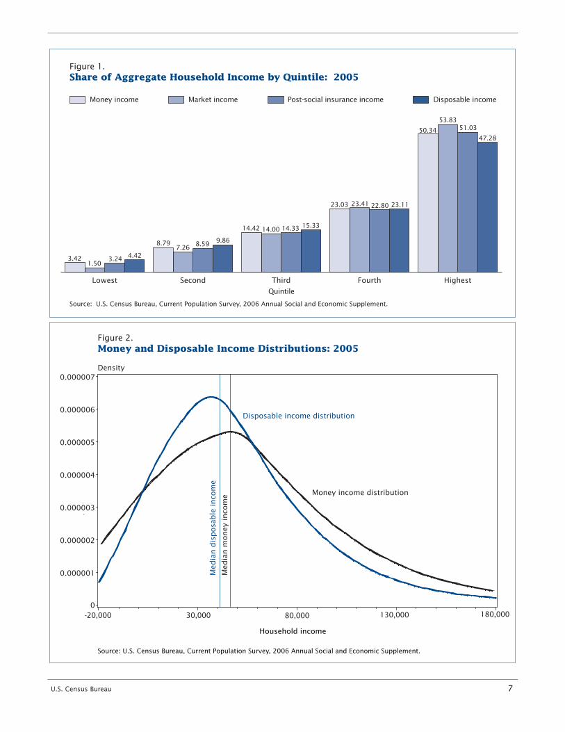
Two widely used measures ofincome inequality are the shares ofaggregate income and the GiniIndex. The shares of aggregateincome are presented by quintileand are derived by dividing aggre-gate income for each quintile byoverall aggregate householdincome. The Gini Index summa-rizes the dispersion of income andranges from 0 (indicating perfectequality) to 1 (indicating perfectinequality). Table 3 presents thesetwo measures of income inequalityfor each income definition. Theshare of aggregate income held bythe lowest quintile is largest underthe disposable income definition.Conversely, the disposable incomedefinition shows the smallest shareof aggregate household income forthe highest quintile. Comparing thedistributions by income definitionsshows how government programsredistribute income. The distribu-tion of income under the marketdefinition is more unequal thanunder the money income definition.The Gini Index for money income is0.450, and for market income it is9.6 percent higher at 0.493. Figure 1 shows that under the mar-ket income definition, the lowestthree quintiles have a smaller shareof aggregate income than underany of the other three income defi-nitions, and the top quintile has thelargest share shown under any ofthe definitions. The Gini Indexunder the disposable income defini-tion was 0.418, showing the mostequal income distribution.

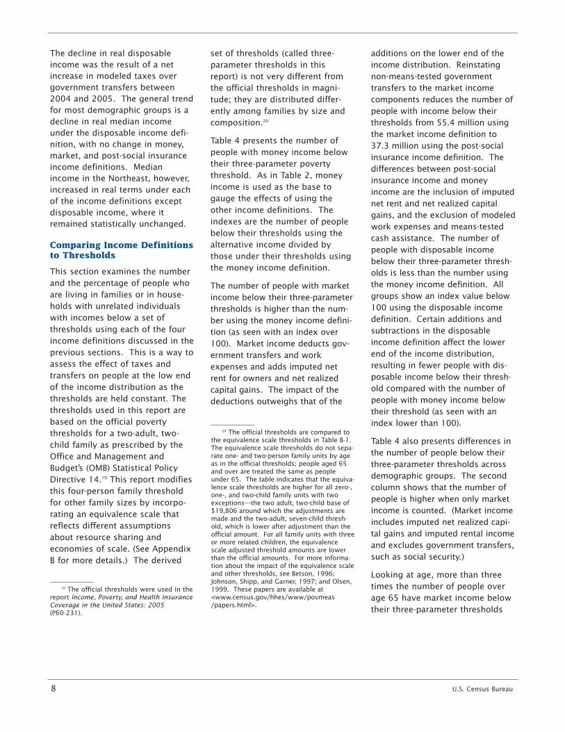
Figure 2 shows the income densityfunctions for money income anddisposable income, illustrating theimpact taxes and transfers have on

the entire income distribution.Household income is on the hori-zontal axis. The vertical axis indi-cates the frequency at which thevalue occurs in the data.17 Thearea under each curve is equal to 1. Using the disposable incomedefinition (the blue density func-tion), the overall distribution slidesto the left and compresses, exhibit-ing less variance around itsmedian. As the figure shows,there are more households in themiddle and fewer in the lower andupper sections using the dispos-able income definition. This illus-trates the redistributional effect ofgovernment taxes and transfersresulting in less inequality usingthe disposable income definitionthan using the money income defi-nition. The additions and subtrac-tions used to construct disposableincome have a differential impacton various segments of the incomedistribution. Under the disposableincome definition, the density isincreased between zero and themedian. The increased area underthe disposable income curve indi-


17 To plot the income distributions usingall weighted ASEC households, a smoothingfunction in SAS is employed to determine theprobability that a particular income valueoccurs. To display all probabilities, the den-sity of each income amount is plotted, form-ing the distribution. The vertical axis islabeled “Density” since this continuous distri-bution is determined by a statistical func-tion. Similarly, if discrete observations wereplotted using a bar graph, the vertical axiswould be labeled “Frequency.”

cates that more households haveincome between 0 and $40,843.This is due to the redistributionaleffects of the additions (noncashtransfers and net realized capitalgains) and subtractions (workexpenses and all taxes) under thedisposable income definition.Above $60,000, the densitydecreases under the disposableincome definition; there is lessarea under the disposable incomecurve compared with the areaunder the money income curve,indicating fewer households. Thistrend continues to the high end ofthe income distribution, indicatingthe impact of progressive taxes.

Comparing the 2005 data to theprevious year, there are changes inreal median household incomesunder the money income and dis-posable income definitions for allhouseholds (Table A-1).18 Moneyincome increased 1.1 percent anddisposable income decreased 1.5percent between 2004 and 2005.

18 All income values are adjusted to reflect2005 dollars. “Real” refers to income afteradjusting for inflation. The adjustment isbased on percentage changes in pricesbetween earlier years and 2005 and is com-puted by dividing the annual averageConsumer Price Index Research Series (CPI-U-RS) for 2005 by the annual average for earlieryears. The CPI-U-RS values for 1947 to 2005are available on the Internet at <www.census.gov/hhes/www/income/income05/cpiurs.html>. Inflation between2004 and 2005 was 3.3 percent. See the textbox “What Are the CPI-U and the CPI-U-RS?” onp. 14 for more information on the CPI-U-RS.

Table 3.Share of Aggregate Household Income by Quintile and theGini Index: 2005

Post-socialQuintile Money Market insurance Disposable

income income income income

Lowest . . . . . . . . . . . . . . . . . . . . . . . . . . . 3.42 1.50 3.24 4.42Second . . . . . . . . . . . . . . . . . . . . . . . . . . . 8.79 7.26 8.59 9.86Third . . . . . . . . . . . . . . . . . . . . . . . . . . . . . 14.42 14.00 14.33 15.33Fourth . . . . . . . . . . . . . . . . . . . . . . . . . . . . 23.03 23.41 22.80 23.11Highest . . . . . . . . . . . . . . . . . . . . . . . . . . . 50.34 53.83 51.03 47.28

Gini index . . . . . . . . . . . . . . . . . . . . . . . . . 0.450 0.493 0.447 0.418

Source: U.S. Census Bureau, Current Population Survey, 2006 Annual Social and EconomicSupplement.


Figure 1.Share of Aggregate Household Income by Quintile: 2005


HighestFourthThirdSecondLowest

Disposable incomeMoney income Market income Post-social insurance income

Quintile

47.28

3.42

8.79

14.42

23.03

50.34

1.50

7.26

14.00

23.41

53.83

3.24

8.59

14.33

22.80

51.03

4.42

9.86

15.33

23.11

Figure 2.Money and Disposable Income Distributions: 2005


Household income

Density

Disposable income distribution

Money income distribution

Med

ian d

isposa

ble

inco

me

Med

ian m

oney

inco

me

0.000007

0.000006

0.000005

0.000004

0.000003

0.000002

0.000001

0-20,000 30,000 80,000 130,000 180,000

The decline in real disposableincome was the result of a netincrease in modeled taxes overgovernment transfers between2004 and 2005. The general trendfor most demographic groups is adecline in real median incomeunder the disposable income defi-nition, with no change in money,market, and post-social insuranceincome definitions. Medianincome in the Northeast, however,increased in real terms under eachof the income definitions exceptdisposable income, where itremained statistically unchanged.

Comparing Income Definitionsto Thresholds

This section examines the numberand the percentage of people whoare living in families or in house-holds with unrelated individualswith incomes below a set ofthresholds using each of the fourincome definitions discussed in theprevious sections. This is a way toassess the effect of taxes andtransfers on people at the low endof the income distribution as thethresholds are held constant. Thethresholds used in this report arebased on the official povertythresholds for a two-adult, two-child family as prescribed by theOffice and Management andBudget’s (OMB) Statistical PolicyDirective 14.19 This report modifiesthis four-person family thresholdfor other family sizes by incorpo-rating an equivalence scale thatreflects different assumptionsabout resource sharing andeconomies of scale. (See AppendixB for more details.) The derived


19 The official thresholds were used in thereport Income, Poverty, and Health InsuranceCoverage in the United States: 2005 (P60-231).

set of thresholds (called three-parameter thresholds in thisreport) is not very different fromthe official thresholds in magni-tude; they are distributed differ-ently among families by size andcomposition.20

Table 4 presents the number ofpeople with money income belowtheir three-parameter povertythreshold. As in Table 2, moneyincome is used as the base togauge the effects of using theother income definitions. Theindexes are the number of peoplebelow their thresholds using thealternative income divided bythose under their thresholds usingthe money income definition.

The number of people with marketincome below their three-parameterthresholds is higher than the num-ber using the money income defini-tion (as seen with an index over100). Market income deducts gov-ernment transfers and workexpenses and adds imputed netrent for owners and net realizedcapital gains. The impact of thedeductions outweighs that of the

20 The official thresholds are compared tothe equivalence scale thresholds in Table B-1.The equivalence scale thresholds do not sepa-rate one- and two-person family units by ageas in the official thresholds; people aged 65and over are treated the same as peopleunder 65. The table indicates that the equiva-lence scale thresholds are higher for all zero-,one-, and two-child family units with twoexceptions—the two adult, two-child base of$19,806 around which the adjustments aremade and the two-adult, seven-child thresh-old, which is lower after adjustment than theofficial amount. For all family units with threeor more related children, the equivalencescale adjusted threshold amounts are lowerthan the official amounts. For more informa-tion about the impact of the equivalence scaleand other thresholds, see Betson, 1996;Johnson, Shipp, and Garner, 1997; and Olsen,1999. These papers are available at <www.census.gov/hhes/www/povmeas/papers.html>.

additions on the lower end of theincome distribution. Reinstatingnon-means-tested governmenttransfers to the market incomecomponents reduces the number ofpeople with income below theirthresholds from 55.4 million usingthe market income definition to37.3 million using the post-socialinsurance income definition. Thedifferences between post-socialinsurance income and moneyincome are the inclusion of imputednet rent and net realized capitalgains, and the exclusion of modeledwork expenses and means-testedcash assistance. The number ofpeople with disposable incomebelow their three-parameter thresh-olds is less than the number usingthe money income definition. Allgroups show an index value below100 using the disposable incomedefinition. Certain additions andsubtractions in the disposableincome definition affect the lowerend of the income distribution,resulting in fewer people with dis-posable income below their thresh-old compared with the number ofpeople with money income belowtheir threshold (as seen with anindex lower than 100).

Table 4 also presents differences inthe number of people below theirthree-parameter thresholds acrossdemographic groups. The secondcolumn shows that the number ofpeople is higher when only marketincome is counted. (Market incomeincludes imputed net realized capi-tal gains and imputed rental incomeand excludes government transfers,such as social security.)

Looking at age, more than threetimes the number of people overage 65 have market income belowtheir three-parameter thresholds

than below their money incomethreshold. The majority of people65 and older receive some incomefrom government transfer pro-grams such as social security, andgovernment transfer payments aresubtracted from money income toform market income. Imputed netrealized capital gains and imputedrental income on owner-occupiedhomes are included in the marketincome definition. These twoimputed income sources generallybenefit those in the 65 and oldercategory who are retired and may

live in their own (paid-in-full)homes.21 Since the number of peo-ple 65 and older who are belowtheir three-parameter thresholds is


21 If imputed net rent is excluded fromthe market income definition, the number ofpeople with disposable income below theirthresholds is 32.7 million. This is an 8.6percent increase over the number of peoplebelow their thresholds when imputed netrent is included. Looking specifically at peo-ple aged 65 and over, excluding the net rentvalue increases the number below theirthresholds by 41.8 percent (from 2.4 millionto 3.4 million). A summary of this data,excluding imputed net rent, is available at<www.census.gov/hhes/www/povmeas/povmeas.html>.

higher using market income, theomission of social security in thisdefinition has a larger impact thanthe inclusion of the imputed rentalincome and realized capital gainson people 65 and older.

Differences among people by fam-ily status are driven by the preva-lence of female householder withno husband present families. Ofthe 26.9 million people in familieswith money income below theirthresholds, 13.4 million, or about50 percent, are living in family

Table 4.People With Income Below the Three-Parameter Thresholds by Selected Characteristicand Income Definition: 2005(Numbers in thousands. People as of March of the following year)

Characteristic Number withmoney income

below theirthresholds

Ratio of the number of people below the threshold underalternative income definitions to the number below the

threshold using money income definition

Marketincome

Post-socialinsurance

incomeDisposable

income

Total1 . . . . . . . . . . . . . . . . . . . . . . . . . . . . . . . . . . . . . . .

Age

36,804 150.4 101.4 81.7

Under 18 years . . . . . . . . . . . . . . . . . . . . . . . . . . . . . . . . . . . . . . . 12,764 115.4 104.4 74.418 to 64 years . . . . . . . . . . . . . . . . . . . . . . . . . . . . . . . . . . . . . . . . 20,234 133.1 104.3 89.965 years and older . . . . . . . . . . . . . . . . . . . . . . . . . . . . . . . . . . . .

Family Status

3,805 360.1 75.6 62.8

In families . . . . . . . . . . . . . . . . . . . . . . . . . . . . . . . . . . . . . . . . . . . 26,923 146.0 102.5 78.1Married-couple families . . . . . . . . . . . . . . . . . . . . . . . . . . . . . . 11,505 174.3 99.3 76.1Female householder, no husband present . . . . . . . . . . . . . 13,401 122.7 104.8 78.3

Unrelated individuals . . . . . . . . . . . . . . . . . . . . . . . . . . . . . . . . . .


9,424 164.7 97.6 91.3

White . . . . . . . . . . . . . . . . . . . . . . . . . . . . . . . . . . . . . . . . . . . . . . . 24,604 160.5 99.9 82.4White, not Hispanic . . . . . . . . . . . . . . . . . . . . . . . . . . . . . . . . . 16,011 181.2 97.0 82.9

Black . . . . . . . . . . . . . . . . . . . . . . . . . . . . . . . . . . . . . . . . . . . . . . . . 9,251 130.6 103.9 79.2Asian . . . . . . . . . . . . . . . . . . . . . . . . . . . . . . . . . . . . . . . . . . . . . . . . 1,436 127.7 105.4 88.2

Hispanic (any race) . . . . . . . . . . . . . . . . . . . . . . . . . . . . . . . . . . .

Educational Attainment(People 25 years and older)

9,335 121.8 105.7 81.6

Less than 12th grade, no diploma . . . . . . . . . . . . . . . . . . . . . . 6,788 170.4 100.7 77.2High school graduate, no college . . . . . . . . . . . . . . . . . . . . . . . 6,618 196.6 98.3 83.9Some college, less than bachelor’s degree . . . . . . . . . . . . . . 3,710 180.1 96.4 85.0Bachelor’s degree or higher . . . . . . . . . . . . . . . . . . . . . . . . . . . . 1,894 176.5 88.8 85.2

1 Details may not sum to total because of rounding or omitted groups.2 Federal surveys now give respondents the option of reporting more than one race. Therefore, two basic ways of defining a race group are possible. A

group such as Asian may be defined as those who reported Asian and no other race (the race-alone or single-race concept) or as those who reported Asianregardless of whether they also reported another race (the race-alone-or-in-combination concept). This table shows data using the first approach (race alone).The use of the single-race population does not imply that it is the preferred method of presenting or analyzing data. The Census Bureau uses a variety ofapproaches. Information on people who reported more than one race, such as White and Asian or Asian and Black or African American, is available fromCensus 2000 through American FactFinder. About 2.6 percent of people reported more than one race in Census 2000.


units with a female householderwith no husband present. Usingthe post-social insurance incomedefinition, people in female house-holder with no husband presentfamilies have an index value of104.8, meaning that, among peo-ple in this family type, more haveincome below their threshold thanwould be below their thresholdunder the money income defini-tion. This 4.8 percentage-pointincrease over the money incomedefinition base captures the exclu-sion of cash means-tested govern-ment transfers, particularly publicassistance that includes TANF, fromthe resource definition.

The final column in Table 4 displaysthe most comprehensive measureof income, disposable income. Thisdefinition expands on thosedetailed thus far by incorporatingnoncash transfers and deducting alltaxes. The net effect of these addi-tions and subtractions moves peo-ple of all characteristics below the100.0 base of money income. Thelargest reduction is for those 65and older. This definition reflectsthe impact of noncash governmenttransfers, as well as tax creditssuch as the Earned Income TaxCredit and the Additional Child TaxCredit, which specifically target low-income people.

Table 5 shows that using dispos-able income instead of moneyincome lowers the percentage ofpeople below their three-parameterthresholds from 12.6 percent to10.3 percent, a 2.3 percentage-point decline.22 This follows sincemore resources have been incorpo-rated into the income definitionthan have been subtracted for


22 If child-care expenses are included inwork expenses, the percentage of peoplewith disposable income below their thresh-olds is 10.5 percent rather than the 10.3percent in the text above. A summary ofthis data, with modeled child-care expenses,is available at <www.census.gov/hhes/www/povmeas/povmeas.html>.

those at the lower end of theincome distribution.

Table 5 displays the percentage ofpeople below their three-parameterthresholds for selected characteris-tics using the money income anddisposable income definitions.Female householders with no hus-bands present show a 6.9percentage-point differencebetween the money income and dis-posable income definitions (31.7percent and 24.8 percent, respec-tively). The proportion of peoplewith fewer than 12 years of educa-tion below their thresholds was 5.5

percentage points lower under thedisposable income definition thanunder the money income definition.The difference in the percentagebelow their thresholds between def-initions was larger for Blacks (5.2percentage points) and Hispanics(4.0 percentage points) than fornon-Hispanic Whites and Asians(both approximately 1.3 percentagepoints).23 Looking at the agecategories, the disposable income

23 The difference in the rates for Blacks(5.2 percentage points) is not statisticallydifferent from the difference in the rates forpeople with less than 12 years of education(5.5 percentage points).

Table 5.The Percentage of People Below the Three-ParameterThresholds by Selected Characteristic and IncomeDefinition: 2005(People as of March of the following year)

Characteristic Moneyincome

Disposableincome

Total . . . . . . . . . . . . . . . . . . . . . . . . . . . . . . . . . . .

Age

12.6 10.3

Under 18 years . . . . . . . . . . . . . . . . . . . . . . . . . . . . . . . . . . 17.4 13.018 to 64 years . . . . . . . . . . . . . . . . . . . . . . . . . . . . . . . . . . . 11.0 9.965 years and older . . . . . . . . . . . . . . . . . . . . . . . . . . . . . . .

Family Status

10.7 6.7

In families . . . . . . . . . . . . . . . . . . . . . . . . . . . . . . . . . . . . . . . 11.1 8.7Married-couple families . . . . . . . . . . . . . . . . . . . . . . . . . 6.2 4.7Female householder, no husband present . . . . . . . . . 31.7 24.8

Unrelated individuals . . . . . . . . . . . . . . . . . . . . . . . . . . . . .


19.0 17.4

White . . . . . . . . . . . . . . . . . . . . . . . . . . . . . . . . . . . . . . . . . . . 10.5 8.6White, not Hispanic . . . . . . . . . . . . . . . . . . . . . . . . . . . . 8.2 6.8

Black . . . . . . . . . . . . . . . . . . . . . . . . . . . . . . . . . . . . . . . . . . . 25.1 19.9Asian . . . . . . . . . . . . . . . . . . . . . . . . . . . . . . . . . . . . . . . . . . . 11.4 10.1

Hispanic (any race) . . . . . . . . . . . . . . . . . . . . . . . . . . . . . .

Educational Attainment(People 25 years and older)

21.7 17.7

Less than 12th grade, no diploma . . . . . . . . . . . . . . . . . . 24.3 18.8High school graduate, no college . . . . . . . . . . . . . . . . . . . 10.9 9.1Some college, less than bachelor’s degree . . . . . . . . . . 7.5 6.4Bachelor’s degree or higher . . . . . . . . . . . . . . . . . . . . . . . 3.5 3.0

1 Federal surveys now give respondents the option of reporting more than one race. Therefore, twobasic ways of defining a race group are possible. A group such as Asian may be defined as those whoreported Asian and no other race (the race-alone or single-race concept) or as those who reported Asianregardless of whether they also reported another race (the race-alone-or-in-combination concept). Thistable shows data using the first approach (race alone). The use of the single-race population does notimply that it is the preferred method of presenting or analyzing data. The Census Bureau uses a varietyof approaches. Information on people who reported more than one race, such as White and Asian orAsian and Black or African American, is available from Census 2000 through American FactFinder.About 2.6 percent of people reported more than one race in Census 2000.

Source: U.S. Census Bureau, Current Population Survey, 2006 Annual Social and EconomicSupplement.

definition shows a lower percentage group regardless of income defini- thresholds. The number of peoplefor all three age groups. tion. Using the money income def- 65 and older below their thresh-

inition, they compose 36.4 percent olds fell 2.4 percentage pointsFigure 3 shows the breakdown of

of all people below their thresh- (from 10.3 percent to 7.9 percent)the population below their three-

olds. Using the disposable income using the inclusive disposableparameter thresholds using money

definition, they compose 34.9 per- income definition, which incorpo-income and disposable income by

cent of the people below their rates all transfers, taxes, andselected characteristics. The bars

three-parameter thresholds. imputed rental income, comparedare different heights because, by

with using money income.construction, fewer people have The young and the old benefitincome below their three-parameter from the inclusion of more Data are presented for incomethreshold using the disposable resources, such as imputed rental years 2004 and 2005 in Table A-2.income definition. income and noncash transfers. For the total poverty universe, no

People under 18 years old repre- significant changes occurredPeople in female householder with

sent 34.7 percent of the popula- across all four definitions betweenno husband present families have

tion with money income less than 2004 and 2005. Changes acrossa lower percentage below their

their thresholds and 31.6 percent demographic characteristics, suchthree-parameter thresholds when

of the population with disposable as the increase in poverty forthe disposable income definition is

income (which includes the value female householder with noused, and they remain the largest

of noncash transfers) below their husband present families from


Figure 3.Population Below the Three-Parameter Thresholds Using Money Income and Disposable Income—Distribution by Selected Characteristic: 2005


0

10

20

30

40

Disposableincome

Moneyincome

0

10

20

30

40

Disposableincome

Moneyincome

0

10

20

30

40

Disposableincome

Moneyincome

Family status Educational attainment Age

Population in thousands Population in thousands Population in thousands

Unrelated individualsMale householder, no wife presentFemale householder, no husband presentMarried-couple family

Bachelor's degree or higherSome college, less than bachelor's degreeHigh school graduate, no collegeLess than 12th grade, no diploma

65 years and older18 to 64 yearsUnder 18 years

35.7% 33.7%

34.8%

35.7%

19.5%

20.3%

10.0%

10.4%

31.3%29.1%

36.4%

34.9%

5.5%

5.9%

25.6%

28.6%

34.7%31.6%

55.0%

60.5%

10.3%

7.9%

2004 to 2005 across all defini- concept with the official poverty definitions when holding thetions, can also be determined from thresholds to determine eligibility thresholds constant. The areaTable A-2. for various programs. For instance, under the curve to the left of the

the food stamp program determines vertical line at 1.0 illustrates theAnother way to view income distri-

eligibility for people below 130 per- population below the thresholds—bution is by calculating income-to-

cent of the federal poverty guide- 36.8 million people using moneythreshold ratios (ITR). Since this

lines, and free school lunches are income and 30.1 million peoplereport uses four income definitions

available to families with income using disposable income (Table 6).and one set of thresholds, four

below 180 percent of the federal The area between the curves to theratios are possible, where the

poverty guidelines. left of the 1.0 vertical line repre-numerator varies by the definition

sents the people who are no longerand the denominator stays the Figure 4 illustrates the distribution below the threshold if the dispos-same. If income is below a given of people according to their ITR for able income definition is used butthreshold, then the ITR is less than the money income and disposable remain below the threshold if the1.0. Values at or above 1.0 indicate income definitions. The two money income definition is used,that income is equal to or greater curves show that the number of indicating the impact of taxes andthan the threshold. Federal and people with income below the transfers on income distributions. state governments use this ratio thresholds varies between the


ITR using money income

ITR using disposable income

ITR=

0.88

ITR=

1

ITR=

1.15

Figure 4.Distributions of Income-to-Threshold Ratios by Income Definition: 2005

Density

Income-to-threshold ratio


0.28

0.26

0.24

0.22

0.20

0.18

0.16

0.14

0.12

0.10

0.08

0.06

0.04

0.020 0.5 1.0 1.5 2.0 2.5 3.0 3.5 4.0 4.5 5.0

The ratios can also be used to illus- of the CPI-U. Similar to the income amount that is 115 percent of thetrate the impact of changing the distributions shown in Figure 2, the 100 percent three-parameterthreshold amounts to revise the ITR distributions indicate that dis- thresholds used elsewhere in thisconcept of need to 2005 standards posable income is less dispersed report. The 115 percent level isor to update the threshold amounts than money income. As in Figure 2, based on the approximate increaseby a different CPI index. Figure 4 the area under each curve sums in real median family income forand Table 6 show the impact of to 1. As seen in Table 6, using the four-person families from 1978 toraising and lowering the thresholds. 88 percent ITR lowers the percent- 2005 using the CPI-U. At 1.15 onIf the thresholds are updated using age of people with money income Figure 4, the disposable incomethe CPI-U-RS instead of the CPI-U, below their threshold from curve is higher than the moneythe amounts are 12 percent lower, 12.6 percent to 10.5 percent and income curve, but the area underresulting in a threshold amount that the percentage with disposable the curves—representing the totalis 88 percent of the 100 percent income below their threshold from number of people with ITR lessthree-parameter thresholds used in 10.3 percent to 8.2 percent. These than 1.15—still finds more peoplethis report. (See the text box “What results are intuitive, as incomes are below the inflation-adjusted 1.15Are the CPI-U and the CPI-U-RS” for being compared against a lower ITR using the money income defini-more information.) The line labeled dollar amount. tion. The higher threshold0.88 on Figure 4 represents this increases the percentage of people

If the thresholds are modified toinflation adjustment. Under both with money income and the per-

incorporate income growth overincome definitions, the number of centage with disposable income

the past several decades, thepeople below their thresholds is below their threshold, as seen in

amounts would be 15 percentlower if the CPI-U-RS is used instead Table 6.

higher, resulting in a threshold


Table 6.People With Income Below Specified Ratios of Their Three-Parameter Thresholds byDefinition of Income: 2005(Numbers in thousands. People as of March of the following year)

Definition of income

Income-to-threshold ratio

Under 0.88 Under 1.00 Under 1.15

Number Percentage Number Percentage Number Percentage

Money income . . . . . . . . . . . . . . . . . . . . . . . . . . .Market income . . . . . . . . . . . . . . . . . . . . . . . . . . .Post-social insurance income . . . . . . . . . . . . . .Disposable income . . . . . . . . . . . . . . . . . . . . . . . .

30,89649,64031,84824,059

10.516.910.9

8.2

36,80455,36937,30630,075

12.618.912.710.3

44,84462,27244,12039,075

15.321.215.113.3


The CPI-U (Consumer Price Index for All UrbanConsumers) and the CPI-U-RS (Consumer Price IndexResearch Series Using Current Methods) are both priceindexes used to update dollar figures for inflation.These indexes are computed by the Bureau of LaborStatistics (BLS) to track the average change in pricesfor consumer goods and services used for consump-tion. More than 200 categories are tracked for theCPI, including food and beverages, housing, apparel,transportation, medical care, recreation, and educa-tion. The index does not include taxes or invest-ments such as stocks, real estate, or life insurance.

The CPI-U is used to update the official povertythresholds for inflation. This means that each yearsince 1967 the poverty thresholds have beenupdated to a higher level using the change in theCPI-U. Statistical Policy Directive 14, issued by theOffice of Management and Budget (OMB), states thatthe official poverty measure is to be updated this way.

The CPI-U-RS is an inflation index covering 1978 tothe present. It applies most of the methodologicalimprovements made to the CPI-U since 1978 to everyyear of the series. Among other improvements, theCPI-U-RS retroactively applies the newest methods ofquality adjustment for many items, including per-sonal computers, televisions, apparel, and manyappliances, and it takes better account of how con-sumers might buy lower-priced goods or services toprotect themselves from price increases on similaritems. Dollar figures updated with the CPI-U-RS tendto be lower than those updated with the CPI-U, partlybecause the CPI-U-RS also uses a corrected methodfor calculating homeownership costs.

Although the CPI-U-RS has some limitations, includ-ing being subject to annual revisions, the BLS statesthat “the CPI-U-RS can serve as a valuable proxy forresearchers needing a historical estimate of inflationusing current methods. The direct adjustment ofindividual CPI index series makes this the mostdetailed and systematic estimate available of aconsistent CPI series.” More information about theCPI-U-RS is available on the BLS Web site at<www.bls.gov/cpi/cpirsdc.htm>.

The results in this report use two sets of thresholdsto evaluate the percentage of people living withincomes below these thresholds. Like the officialthresholds, the three-parameter thresholds in thisreport have been updated annually (since 1978)using the CPI-U. An alternative series of thresholdscould also be obtained by using alternative updat-ing methods. One alternative method is to use theCPI-U-RS series to update the thresholds. To pro-duce a series of thresholds, a base year must bechosen. The base year is usually the first year ofanalysis or the most recent year.

Comparing the outcomes when alternative inflationindexes are used to adjust the thresholds highlightsthe effects of the indexes on trends in poverty. Forexample, using 1978 as the base year and adjustingthe three-parameter thresholds each year by thechange in the CPI-U-RS yields thresholds that areslightly lower than the official thresholds in eachsubsequent year. As a result, the 2005 threshold is88 percent of the three-parameter thresholdsupdated using the CPI-U. This is because thechange in the CPI-U-RS between 1978 and 2005 islower than the change in the CPI-U during this time.As Figure 5 shows, the resulting series of the per-centage of people living below these thresholds isalso lower than the rates using the CPI-U.

Alternatively, the current year (2005) can be used asthe base year. Following the treatment of income inthe report Income, Poverty, and Health InsuranceCoverage in the United States: 2005 (P60-231), thecurrent (2005) poverty thresholds could be adjustedback to 1978 using the CPI-U-RS. Because the CPI-U-RS increases less than the CPI-U, the poverty thresh-olds in 1978 would be higher than the thresholdsobtained using the CPI-U, which yields a higher per-centage of people living with incomes below thesethresholds. The trends in both series are similar nomatter which base period is used. Both trends,however, differ from the trend using the CPI-U.Using the CPI-U-RS yields a slight decrease inpoverty between 1978 and 2005, while the CPI-Uyields an increase between these 2 years.

WHAT ARE THE CPI-U AND THE CPI-U-RS?


SOURCE OF THE DATA The estimates in this report (which CPS DATA COLLECTION AND ACCURACY OF may be shown in text, figures, and

The information in this report wasTHE ESTIMATES tables) are based on responses collected in the 50 states and the

from a sample of the populationThe data in this report are from the District of Columbia and does notand may differ from actual valuesASEC to the 2005 and 2006 CPS con- represent residents of Puerto Ricobecause of sampling variability orducted by the Census Bureau. The and U.S. island areas. It is based

population represented in the survey other factors. As a result, apparent on a sample of about 100,000(the population universe) is the civil- differences between the estimates addresses. The estimates in thisian noninstitutionalized population for two or more groups may not be report are controlled to nationalliving in the United States. Members statistically significant. All compar- population estimates by age, race,of the armed forces living off post or ative statements have undergone sex, and Hispanic origin and towith their families on post are statistical testing and are signifi- state population estimates by age,included if at least one civilian adult cant at the 90-percent confidence race, and sex. The population con-lives in the household. Most of the level unless otherwise noted. trols used to prepare estimates fordata from the CPS ASEC were col- Further information about the 1999 to 2006 were based on thelected in March (with some data col- source and accuracy of the esti- results from Census 2000 and arelected in February and April), and the mates is available at updated annually using administra-data were controlled to independent <www.census.gov/hhes/www tive records such as birth andpopulation estimates for March of /income/p60_231sa.pdf>. death certificates. the survey year.


Figure 5.Percentage of People Below Their Three-Parameter Thresholds: 1978–2005

Note: The data points are placed at the midpoints of the respective years.Source: U.S. Census Bureau, Current Population Survey, 1979 to 2006 Annual Social and Economic Supplements.

0

3

6

9

12

15

18

2005200219991996199319901987198419811978

Percent

Three-parameter thresholds (CPI-U-RS from 2005)

Three-parameter thresholds (CPI-U from 1978)Three-parameter thresholds (CPI-U-RS from 1978)

The CPS is a household survey pri- eligible to be interviewed in the live in a household with at leastmarily used to collect employment CPS. Students living in dormitories one other civilian adult, regardlessdata. The sample universe for the are only included in the estimates of whether they live off post or onbasic CPS consists of the resident if information about them is post. All other armed forces arecivilian noninstitutionalized popu- reported in an interview at their excluded. For further documenta-lation of the United States. People parents’ homes. The sample uni- tion about the CPS ASEC, seein institutions, such as prisons, verse for the CPS ASEC is slightly <www.bls.census.gov/cps/adslong-term care hospitals, and nurs- larger than the basic CPS since it /adsmain.htm>.ing homes, are therefore not includes military personnel who


REFERENCES

Betson, David. 1996. “Is <www.census.gov/hhes/www Skuterud, Mikal, Marc Frenette, andEverything Relative? The Role of /poverty/poverty05.html >. Preston Poon. 2004.Equivalence Scales in Poverty “Describing the Distribution of

Johnson, David, Stephanie Shipp,Measurement.” University of Income: Guidelines for Effective

and Thesia I. Garner. AugustNotre Dame, unpublished manu- Analysis.” Statistics Canada,

1997. “Developing Povertyscript. Income Research Paper Series.

Thresholds Using ExpenditureCitro, Constance F., and Robert T. Data.” Proceedings of the U.S. Census Bureau. 2006. “The

Michael (eds.). 1995. Measuring Government and Social Statistics Effects of Government TaxesPoverty: A New Approach. Section. Alexandria, VA: and Transfers on Income andWashington, DC: National American Statistical Association, Poverty: 2004.” U.S. CensusAcademy Press. pp. 28–37. Bureau Internet Release.

<www.census.gov/hhesCleveland, Robert W. 2005. O’Hara, Amy. 2004. “New

/www/income/effect2004Alternative Income Estimates in Methods for Simulating CPS

/effect2004.html>.the United States: 2003. U.S. Taxes.” U.S. Census BureauCensus Bureau, Current Technical Paper. U.S. Census Bureau. 1993.Population Reports, P60-228. <www.census.gov/hhes/www Measuring the Effect of BenefitsWashington, DC: U.S. /income/oharataxmodel.pdf>. and Taxes on Income and PovertyGovernment Printing Office. 1992. Current Population

Olsen, Kelly A. 1999. “Application<www.census.gov/prod Reports, P60-186RD.

of Experimental Poverty/2005pubs/p60-228.pdf>. Washington, DC: U.S.

Measures to the Aged.” SocialGovernment Printing Office.

Dalaker, Joe. 2005. Alternative Security Bulletin, Volume 62,<www.census.gov/hhes

Poverty Estimates in the United Number 3./www/poverty/prevcps

States: 2003. U.S. CensusRoemer, Marc. 2000. “Assessing /p60-186rd.pdf>.

Bureau, Current Populationthe Quality of the March Current

Reports, P60-227. Washington, Weinberg, Daniel W. 2005.Population Survey and the

DC: U.S. Government Printing Alternative Measures of IncomeSurvey of Income and Program

Office. <www.census.gov and Poverty and the Anti-PovertyParticipation Income Estimates,

/hhes/www/poverty Effects of Taxes and Transfers.1990–1996.” U.S. Census

/altpovest03/altpovestrpt.html>. CES-5-08. U.S. Census Bureau.Bureau. <www.census.gov/hhes

<http://webserver01.cesDeNavas-Walt, Carmen, Bernadette /www/income/assess1.pdf>.

.census.gov/index.php/ces/1.00D. Proctor, and Cheryl Hill Lee.

Short, Kathleen. 2001. /cespapers?down_key=101716>.2006. Income, Poverty, and

Experimental Poverty Measures:Health Insurance Coverage in

1999. U.S. Census Bureau,the United States: 2005. U.S.

Current Population Reports, Census Bureau, Current

P60-216. Washington, DC: U.S.Population Reports, P60-231.

Government Printing Office.Washington, DC: U.S.

<www.census.gov/prodGovernment Printing Office.

/2001pubs/p60-216.pdf>.

ACKNOWLEDGEMENTS COMMENTS

This report would not have been The Census Bureau welcomes thepossible without the efforts of comments and advice of data and

many dedicated U.S. Census report users. If you have sugges-

Bureau staff members. Amy tions or comments, please write to:

O’Hara, Bernadette D. Proctor, Charles Nelson Jessica Semega, Sharon M. Stern, Assistant Division Chief forand Edward Welniak Jr. all con- Income, Poverty, and Health tributed to the creation of this Statistics report under the overall direction Housing and Household Economic of Charles T. Nelson and David S. Statistics Division Johnson. U.S. Census Bureau

Washington, DC 20233-8500

or send e-mail to <[email protected]>.


Appendix A. DETAILED TABLES


Table A-1.Median Income of Households by Selected Characteristic and Income Definition: 2004and 2005(Households as of March of the following year)

Money Market Post-social insurance Disposableincome income income income(dollars) (dollars) (dollars) (dollars)

CharacteristicNumber 90-percent 90-percent 90-percent 90-percent

(thou- confidence confidence confidence confidencesands) Median interval1 (±) Median interval1 (±) Median interval1 (±) Median interval1 (±)

2005

All households . . . . . . . . . . 114,384 46,326 255 43,701 297 47,975 272 40,843 229

Type of Household

Family households . . . . . . . . . . . . . . . 77,402 57,278 332 55,650 400 59,731 359 50,707 290Married-couple . . . . . . . . . . . . . . . . 58,179 66,067 402 65,564 488 69,349 414 57,786 324Female householder, no husband

present . . . . . . . . . . . . . . . . . . . . . . 14,093 30,650 432 27,107 597 30,419 546 29,464 328Nonfamily households . . . . . . . . . . . . 36,982 27,326 267 24,712 345 29,395 284 25,283 227


White . . . . . . . . . . . . . . . . . . . . . . . . . . 93,588 48,554 349 46,153 371 50,482 348 42,883 245White, not Hispanic . . . . . . . . . . . . 82,003 50,784 283 48,513 350 53,142 363 44,599 261

Black . . . . . . . . . . . . . . . . . . . . . . . . . . . 14,002 30,858 495 27,370 677 30,713 623 28,416 400Asian . . . . . . . . . . . . . . . . . . . . . . . . . . . 4,273 61,094 1,171 61,505 2,507 64,362 1,884 53,051 1,276

Hispanic (any race) . . . . . . . . . . . . . . 12,519 35,967 586 33,730 632 35,744 639 32,769 484

Region

Northeast . . . . . . . . . . . . . . . . . . . . . . . 7,400 50,882 610 48,875 806 53,688 875 44,151 562Midwest . . . . . . . . . . . . . . . . . . . . . . . . 14,904 45,950 578 43,387 562 47,487 548 39,886 410South . . . . . . . . . . . . . . . . . . . . . . . . . . 8,406 42,138 349 39,022 440 43,457 484 37,919 333West . . . . . . . . . . . . . . . . . . . . . . . . . . . 25,174 50,002 608 48,413 644 52,143 662 44,846 526

Number of Earners

No earners . . . . . . . . . . . . . . . . . . . . . . 24,244 16,893 209 6,650 163 20,381 278 19,984 235One earner . . . . . . . . . . . . . . . . . . . . . 42,066 37,541 324 35,565 337 38,719 295 33,027 227Two earners or more . . . . . . . . . . . . . 48,095 75,293 398 75,434 502 77,343 481 62,556 351

Two earners . . . . . . . . . . . . . . . . . . 38,327 70,952 391 71,159 531 72,967 510 59,184 373Three earners . . . . . . . . . . . . . . . . . 7,337 87,905 1,208 88,086 1,155 90,055 1,124 72,998 830Four earners or more . . . . . . . . . . 2,430 100,000 (NA) 100,000 (NA) 100,000 (NA) 87,912 1,991


Worked . . . . . . . . . . . . . . . . . . . . . . . . . 79,087 57,802 446 57,510 358 59,326 354 48,561 276Worked full-time, year-round . . . . 57,418 63,610 480 64,232 423 65,537 448 52,711 331

Did not work . . . . . . . . . . . . . . . . . . . . 35,297 23,801 272 13,973 273 27,421 303 26,487 251

20043 (in 2005 dollars)

All households . . . . . . . . . . 113,343 45,817 333 43,589 307 48,089 309 41,446 228

Type of Household

Family households . . . . . . . . . . . . . . . 76,858 57,179 338 55,645 423 60,148 360 51,656 294Married-couple families . . . . . . . . . 57,975 65,946 489 65,844 492 69,732 477 58,602 327Female householder, no husband

present . . . . . . . . . . . . . . . . . . . . . . 13,981 30,824 530 27,725 587 31,178 543 30,563 356Nonfamily households . . . . . . . . . . . . 36,485 27,128 262 24,738 320 29,237 263 25,205 218


White . . . . . . . . . . . . . . . . . . . . . . . . . . 92,880 48,218 311 46,245 356 50,707 301 43,470 247White, not Hispanic . . . . . . . . . . . . 81,628 50,546 380 48,674 398 53,235 374 45,247 279

Black . . . . . . . . . . . . . . . . . . . . . . . . . . . 13,809 31,102 532 27,785 799 31,175 591 28,931 465Asian . . . . . . . . . . . . . . . . . . . . . . . . . . . 4,123 59,427 2,078 61,771 2,041 63,245 2,190 52,485 1,559

Hispanic (any race) . . . . . . . . . . . . . . 12,178 35,418 816 33,415 697 35,608 586 33,367 459

See footnotes at end of table.


Table A-1.Median Income of Households by Selected Characteristic and Income Definition: 2004and 2005—Con.(Households as of March of the following year)

CharacteristicNumber

(thou-sands)

Moneyincome(dollars)

Marketincome(dollars)

Post-social insuranceincome(dollars)

Disposableincome(dollars)

Median

90-percentconfidence

interval1 (±) Median






interval1 (±)

Region

Northeast . . . . . . . . . . . . . . . . . . . . . . . 21,187 49,462 819 47,700 813 52,477 838 43,949 613Midwest . . . . . . . . . . . . . . . . . . . . . . . . 25,939 46,134 661 43,739 636 48,163 709 40,969 440South . . . . . . . . . . . . . . . . . . . . . . . . . . 41,224 42,108 375 39,326 475 43,512 445 38,375 348West . . . . . . . . . . . . . . . . . . . . . . . . . . . 24,993 49,244 669 47,871 732 52,083 767 45,480 528

Number of Earners

No earners . . . . . . . . . . . . . . . . . . . . . . 23,952 16,667 214 7,344 160 20,664 258 20,284 218One earner . . . . . . . . . . . . . . . . . . . . . 41,799 37,371 254 35,430 273 38,763 310 33,442 222Two earners or more . . . . . . . . . . . . . 47,593 75,024 452 75,744 505 77,728 512 63,841 381

Two earners . . . . . . . . . . . . . . . . . . 38,119 71,224 519 71,689 507 73,528 492 60,346 385Three earners . . . . . . . . . . . . . . . . . 7,202 86,628 1,258 87,908 1,181 89,651 1,135 74,081 1,069Four earners or more . . . . . . . . . . 2,271 100,000 (NA) 100,000 (NA) 100,000 (NA) 90,445 1,739


Worked . . . . . . . . . . . . . . . . . . . . . . . . . 78,490 57,706 328 57,605 433 59,773 346 49,324 300Worked full-time, year-round . . . . 56,605 63,624 301 64,223 402 65,441 416 53,540 312

Did not work . . . . . . . . . . . . . . . . . . . . 34,853 22,951 242 14,068 264 27,123 318 26,283 287

(NA) Not available.1 The 90-percent confidence interval is computed by multiplying the standard errors by 1.645. A 90-percent confidence interval is a measure of an estimate’s

variability. The larger the confidence interval in relation to the size of the estimate, the less reliable the estimate. For more information, see ‘‘Standard Errorsand Their Use’’ at <www.census.gov/hhes/www /p60_231sa.pdf>.

2 Federal surveys now give respondents the option of reporting more than one race. Therefore, two basic ways of defining a race group are possible. Agroup such as Asian may be defined as those who reported Asian and no other race (the race-alone or single-race concept) or as those who reported Asianregardless of whether they also reported another race (the race-alone-or-in-combination concept). This table shows data using the first approach (race alone).The use of the single-race population does not imply that it is the preferred method of presenting or analyzing data. The Census Bureau uses a variety ofapproaches. Information on people who reported more than one race, such as White and Asian or Asian and Black or African American, is available fromCensus 2000 through American FactFinder. About 2.6 percent of people reported more than one race in Census 2000.

3 The 2004 data have been revised to reflect a correction to the weights in the 2005 ASEC.Source: U.S. Census Bureau, Current Population Survey, 2005 and 2006 Annual Social and Economic Supplements.


Table A-2.Number and Percentage of People With Alternative Definitions of Income Below theThree-Parameter Poverty Thresholds by Selected Characteristic: 2004 and 2005(Numbers in thousands, confidence intervals (C.I.) in thousands or percentage points as appropriate. People as of March of the following year)

Characteristic

Total

Money income Market income Post-social insurance income Disposable income

Num-ber

belowthresh-

old

90-per-cent

C.I.1(±)

Per-cent-age

belowthresh-

old

90-per-cent

C.I.1(±)

Num-ber

belowthresh-

old

90-per-cent

C.I.1(±)

Per-cent-age

belowthresh-

old

90-per-cent

C.I.1(±)

Num-ber

belowthresh-

old

90-per-cent

C.I.1(±)

Per-cent-age

belowthresh-

old

90-per-cent

C.I.1(±)

Num-ber

belowthresh-

old

90-per-cent

C.I.1(±)

Per-cent-age

belowthresh-

old

90-percentC.I.1(±)

2005Total2 . . . . . . . .

Age

293,135 36,804 678 12.6 0.2 55,369 801 18.9 0.3 37,306 682 12.7 0.2 30,075 621 10.3 0.2

Under 18 years . . . . . . . . 73,285 12,764 344 17.4 0.5 14,731 365 20.1 0.5 13,321 350 18.2 0.5 9,495 304 13.0 0.418 to 64 years . . . . . . . . . 184,345 20,235 514 11.0 0.3 26,936 583 14.6 0.3 21,109 523 11.5 0.3 18,191 489 9.9 0.365 years and older . . . . .

Family Status

35,505 3,805 136 10.7 0.4 13,701 214 38.6 0.6 2,876 120 8.1 0.3 2,389 110 6.7 0.3

In families . . . . . . . . . . . . 242,389 26,923 591 11.1 0.2 39,319 698 16.2 0.3 27,602 598 11.4 0.2 21,039 528 8.7 0.2Married-couple families. .Female householder, no

185,723 11,505 397 6.2 0.2 20,051 517 10.8 0.3 11,429 396 6.2 0.2 8,757 348 4.7 0.2

husband present . . . . . 42,244 13,401 428 31.7 1.1 16,443 471 38.9 1.2 14,040 437 33.2 1.1 10,496 380 24.8 1.0Unrelated individuals . . . .

Race3 and HispanicOrigin

49,526 9,424 210 19.0 0.4 15,526 293 31.3 0.6 9,197 207 18.6 0.4 8,603 198 17.4 0.4

White . . . . . . . . . . . . . . 235,430 24,604 568 10.5 0.2 39,491 699 16.8 0.3 24,578 567 10.4 0.2 20,275 519 8.6 0.2White, not Hispanic . . . . 195,553 16,011 465 8.2 0.2 29,019 611 14.8 0.3 15,524 458 7.9 0.2 13,272 426 6.8 0.2

Black . . . . . . . . . . . . . . 36,802 9,251 333 25.1 0.9 12,084 369 32.8 1.0 9,612 338 26.1 0.9 7,330 302 19.9 0.8Asian . . . . . . . . . . . . . . 12,580 1,436 138 11.4 1.1 1,834 155 14.6 1.2 1,513 142 12.0 1.1 1,267 130 10.1 1.0

Hispanic (any race) . . . . .

Nativity

43,020 9,335 323 21.7 0.8 11,373 346 26.4 0.8 9,865 330 22.9 0.8 7,622 299 17.7 0.7

Native . . . . . . . . . . . . . . 257,513 30,908 629 12.0 0.2 47,880 757 18.6 0.3 31,121 631 12.1 0.2 24,963 571 9.7 0.2Foreign born . . . . . . . . . .

Educational Attainment(People 25 years andolder)

Less than 12th grade, no

35,621 5,896 328 16.6 1.0 7,489 368 21.0 1.1 6,185 335 17.4 1.0 5,112 306 14.4 0.9

diploma . . . . . . . . . . . .High school graduate, no

27,896 6,788 308 24.3 1.2 11,570 396 41.5 1.5 6,837 308 24.5 1.2 5,238 270 18.8 1.0

college . . . . . . . . . . . . .Some college, less than

60,898 6,618 303 10.9 0.5 13,009 419 21.4 0.7 6,506 301 10.7 0.5 5,553 278 9.1 0.5

bachelor’s degree . . . . .Bachelor’s degree or

49,371 3,710 229 7.5 0.5 6,683 304 13.5 0.7 3,575 224 7.2 0.5 3,153 211 6.4 0.5

higher. . . . . . . . . . . . . .

Region

53,720 1,894 165 3.5 0.3 3,342 217 6.2 0.3 1,682 155 3.1 0.3 1,614 151 3.0 0.3

Northeast . . . . . . . . . . . . 54,010 6,094 285 11.3 0.5 9,353 341 17.3 0.6 6,255 288 11.6 0.5 4,855 257 9.0 0.5Midwest . . . . . . . . . . . . . 64,973 7,400 311 11.4 0.5 11,520 373 17.7 0.6 7,358 310 11.3 0.5 6,103 285 9.4 0.4South . . . . . . . . . . . . . . 106,089 14,904 444 14.0 0.4 22,631 523 21.3 0.5 14,963 445 14.1 0.4 12,237 408 11.5 0.4West . . . . . . . . . . . . . . .

20044

68,063 8,406 340 12.4 0.5 11,865 392 17.4 0.6 8,729 345 12.8 0.5 6,880 311 10.1 0.5

Total2 . . . . . . . .

Age

290,617 36,764 678 12.7 0.2 54,550 797 18.8 0.3 36,595 677 12.6 0.2 29,488 616 10.1 0.2

Under 18 years . . . . . . . . 73,241 12,736 345 17.4 0.5 14,628 364 20.0 0.5 13,117 349 17.9 0.5 9,366 303 12.8 0.418 to 64 years . . . . . . . . 182,166 20,330 517 11.2 0.3 26,521 582 14.6 0.3 20,788 522 11.4 0.3 17,854 487 9.8 0.365 years and older . . . . .

Family Status

35,209 3,697 134 10.5 0.4 13,401 210 38.1 0.6 2,690 116 7.6 0.3 2,267 107 6.4 0.3

In families . . . . . . . . . . . 240,754 27,045 592 11.2 0.2 39,116 696 16.2 0.3 27,201 594 11.3 0.2 20,709 525 8.6 0.2Married-couple families. .Female householder, no

184,772 12,017 406 6.5 0.2 20,454 522 11.1 0.3 11,687 400 6.3 0.2 9,034 354 4.9 0.2

husband present . . . . . 42,053 13,034 422 31.0 1.1 15,962 464 38.0 1.2 13,479 429 32.1 1.1 9,981 371 23.7 0.9Unrelated individuals . . . .

Race3 and HispanicOrigin

48,609 9,141 206 18.8 0.4 14,816 284 30.5 0.6 8,794 201 18.1 0.4 8,264 193 17.0 0.4

White . . . . . . . . . . . . . . 233,741 25,073 573 10.7 0.2 39,340 698 16.8 0.3 24,551 567 10.5 0.2 20,167 518 8.6 0.2White, not Hispanic . . . . 195,098 16,718 475 8.6 0.2 29,307 614 15.0 0.3 15,953 464 8.2 0.2 13,551 430 6.9 0.2

Black . . . . . . . . . . . . . . 36,426 8,988 338 24.7 0.9 11,546 376 31.7 1.0 9,153 341 25.1 0.9 7,052 303 19.4 0.8Asian . . . . . . . . . . . . . . 12,231 1,224 131 10.0 1.1 1,678 153 13.7 1.2 1,301 135 10.6 1.1 1,149 127 9.4 1.0

Hispanic (any race) . . . . .

Nativity

41,690 9,053 317 21.7 0.8 10,919 337 26.2 0.8 9,358 320 22.4 0.8 7,134 290 17.1 0.7

Native . . . . . . . . . . . . . . 255,443 30,715 627 12.0 0.2 46,831 750 18.3 0.3 30,253 623 11.8 0.2 24,260 564 9.5 0.2Foreign born . . . . . . . . . .

See footnotes at end of ta

35,173

ble.

6,048 332 17.2 1.0 7,719 374 21.9 1.1 6,342 340 18.0 1.0 5,228 309 14.9 0.9


Table A-2.Number and Percentage of People With Alternative Definitions of Income Below theThree-Parameter Poverty Thresholds by Selected Characteristic: 2004 and 2005—Con.(Numbers in thousands, confidence intervals (C.I.) in thousands or percentage points as appropriate. People as of March of the following year)

Characteristic

Total

Money income Market income Post-social insurance income Disposable income

Num-ber

belowthresh-

old

90-per-cent

C.I.1(±)

Per-cent-age

belowthresh-

old

90-per-cent

C.I.1(±)

Num-ber

belowthresh-

old

90-per-cent

C.I.1(±)

Per-cent-age

belowthresh-

old

90-per-cent

C.I.1(±)

Num-ber

belowthresh-

old

90-per-cent

C.I.1(±)

Per-cent-age

belowthresh-

old

90-per-cent

C.I.1(±)

Num-ber

belowthresh-

old

90-per-cent

C.I.1(±)

Per-cent-age

belowthresh-

old

90-percentC.I.1(±)

Educational Attainment(People 25 years andolder)

Less than 12th grade, nodiploma . . . . . . . . . . . .

High school graduate, no28,015 6,756 306 24.1 1.2 11,583 396 41.3 1.5 6,623 303 23.6 1.2 5,088 266 18.2 1.0

college . . . . . . . . . . . . .Some college, less than

60,893 6,646 304 10.9 0.5 12,746 415 20.9 0.7 6,377 298 10.5 0.5 5,385 275 8.8 0.5

bachelor’s degree . . . . .Bachelor’s degree or

48,077 3,411 219 7.1 0.5 6,245 294 13.0 0.7 3,235 214 6.7 0.5 2,757 197 5.7 0.5

higher . . . . . . . . . . . . .

Region

52,381 2,118 173 4.0 0.3 3,260 214 6.2 0.5 1,843 161 3.5 0.3 1,841 161 3.5 0.3

Northeast . . . . . . . . . . . . 53,906 6,269 279 11.6 0.5 9,242 337 17.1 0.7 6,232 279 11.6 0.5 4,931 248 9.1 0.5Midwest . . . . . . . . . . . . . 64,740 7,430 307 11.5 0.5 11,505 379 17.8 0.6 7,352 305 11.4 0.5 5,922 275 9.1 0.4South . . . . . . . . . . . . . . 104,887 14,848 479 14.2 0.5 22,043 576 21.0 0.6 14,528 474 13.9 0.5 11,979 432 11.4 0.4West . . . . . . . . . . . . . . . 67,083 8,217 375 12.2 0.6 11,760 446 17.5 0.7 8,483 381 12.6 0.6 6,655 338 9.9 0.5

1 The 90-percent confidence interval is computed by multiplying the standard errors by 1.645. A 90-percent confidence interval is a measure of an estimate’s variability. The larger theconfidence interval in relation to the size of the estimate, the less reliable the estimate. For more information, see ‘‘Standard Errors and Their Use’’ at <www.census.gov/hhes/www/p60_231sa.pdf>.

2 Details may not sum to total because of rounding.3 Federal surveys now give respondents the option of reporting more than one race. Therefore, two basic ways of defining a race group are possible. A group such as Asian may be

defined as those who reported Asian and no other race (the race-alone or single-race concept) or as those who reported Asian regardless of whether they also reported another race (therace-alone-or-in-combination concept). This table shows data using the first approach (race alone). The use of the single-race population does not imply that it is the preferred method ofpresenting or analyzing data. The Census Bureau uses a variety of approaches. Information on people who reported more than one race, such as White and Asian or Asian and Black orAfrican American, is available from Census 2000 through American FactFinder. About 2.6 percent of people reported more than one race in Census 2000.

4 The 2004 data have been revised to reflect a correction to the weights in the 2005 ASEC.

Source: U.S. Census Bureau, Current Population Survey, 2005 and 2006 Annual Social and Economic Supplements.


Appendix B. THREE-PARAMETER EQUIVALENCE SCALE POVERTY THRESHOLDS

Official poverty thresholds, those official poverty threshold matrix by thresholds vary as taxes and trans-calculated following the Office of instituting a three-parameter scale, fers are incorporated. Management and Budget’s (OMB) as shown in Table B-1.

Example: Suppose Family A con-Statistical Policy Directive 14, areThe three-parameter scale used here sists of four people: two children,described on the Internet and in thehas the following characteristics: their mother, and their father.report Income, Poverty, and Health

Family A’s poverty threshold inInsurance Coverage in the United • The first parameter reflects that2005 was $19,809. Suppose alsoStates: 2005 (P60-231). The children, on average, consumethat each member had the follow-Census Bureau uses a set of money less than adults.ing income in 2005:thresholds that vary by family size

• The second parameter reflectsand composition to determine who Money Disposablethat as family size increases,is in poverty (Table B-1). Social income incomeexpenses do not increase at theSecurity Administration economistsame rate.Mollie Orshansky devised the Mother $10,000 $10,000

thresholds in the 1960s, based in Father 5,000 15,000• The third parameter allows thelarge part on the U.S. Department of first child in a single-adult fam- First child 0 0Agriculture’s food plan, which ily to represent a larger increase Second child 0 0defined a generally accepted ade- in expenses than the first child

Total: $15,000 $25,000quate amount of food. Although the in a two-adult family.matrix has undergone a few slight Under the money income defini-

For details on the derivation of thisrevisions since then, thresholds tion, the family had total incomeequivalence scale, see Appendix Areflecting a revised concept of need equal to $15,000, which was lessof Short, 2001.(or as Orshansky might have called than their threshold ($19,809);

it “adequacy for essentials of liv- As with the official definition of hence, the people in this familying”) have not been included in the poverty, if a family’s total income is would be counted among thosepoverty series. Instead, for official less than that family’s threshold, with money income less than theirpoverty estimates, the thresholds then that family and every individ- threshold. Under the disposableare updated each year for the cost ual in it is considered below the income definition, the family’s totalof inflation using the Consumer threshold in this report. While the income was $25,000, possibly duePrice Index for All Urban Consumers official poverty definition uses to the inclusion of tax credits, food(CPI-U). For a history of the official money income before taxes and stamps, and housing subsidies.poverty measure, see “The does not include realized capital Since this amount is higher thanDevelopment of the Orshansky gains or the value of noncash ben- their threshold ($19,809), the fam-Thresholds and Their Subsequent efits (such as public housing, ily members would be countedHistory as the Official U.S. Poverty Medicaid, and food stamps), this among those with disposableMeasure” by Gordon Fisher, avail- report compares three alternative income above their thresholds. Forable at <www.census.gov/hhes measures of resources to the same

each calculation, the threshold is/povmeas/papers/orshansky.html>. set of three-parameter scale

the same and only the measure ofAlthough this report does not pro- thresholds to determine how theresources differs. pose a revised poverty measure, it number and characteristics of

does examine a modification to the people with income below the


Table B-1Official Poverty Thresholds and Three-Parameter Scaled Thresholds Used in AlternativePoverty Estimates: 2005(Dollars)

Size of family unit

Number of related children under 18 years

None One Two Three Four Five Six SevenEight or

more

Official Thresholds

One personUnder 65 years . . . . . . . . . . . . . . . . . . . 10,16065 years and older . . . . . . . . . . . . . . . .

Two people

9,367

Householder under 65 years. . . . . . . . 13,078 13,461Householder 65 years and older . . . . 11,805 13,410

Three people . . . . . . . . . . . . . . . . . . . . . . . 15,277 15,720 15,735Four people . . . . . . . . . . . . . . . . . . . . . . . . 20,144 20,474 19,806 19,874Five people . . . . . . . . . . . . . . . . . . . . . . . . . 24,293 24,646 23,891 23,307 22,951Six people . . . . . . . . . . . . . . . . . . . . . . . . . . 27,941 28,052 27,474 26,920 26,096 25,608Seven people . . . . . . . . . . . . . . . . . . . . . . . 32,150 32,350 31,658 31,176 30,277 29,229 28,079Eight people . . . . . . . . . . . . . . . . . . . . . . . . 35,957 36,274 35,621 35,049 34,237 33,207 32,135 31,862Nine people or more . . . . . . . . . . . . . . . . .

Four-Person Threshold With Three-Parameter Equivalence ScaleThresholds

43,254 43,463 42,885 42,400 41,603 40,507 39,515 39,270 37,757

One person. . . . . . . . . . . . . . . . . . . . . . . . . 9,179Two people . . . . . . . . . . . . . . . . . . . . . . . . . 12,943 13,852Three people . . . . . . . . . . . . . . . . . . . . . . . 19,806 17,433 16,445Four people . . . . . . . . . . . . . . . . . . . . . . . . 24,224 22,063 19,806 18,872Five people . . . . . . . . . . . . . . . . . . . . . . . . . 28,320 26,306 24,224 22,063 21,172Six people . . . . . . . . . . . . . . . . . . . . . . . . . . 32,175 30,274 28,320 26,306 24,224 23,370Seven people . . . . . . . . . . . . . . . . . . . . . . . 35,841 34,029 32,175 30,274 28,320 26,306 25,482Eight people . . . . . . . . . . . . . . . . . . . . . . . . 39,353 37,614 35,841 34,029 32,175 30,274 28,320 27,522Nine people or more . . . . . . . . . . . . . . . . . 42,735 41,059 39,353 37,614 35,841 34,029 32,175 30,274 29,499

Source: U.S. Census Bureau.

Income Underreporting in the wage and salary difference wasCPS ASEC around 3 percent while the differ-

ence for transfer incomes wasThe collection vehicle for the esti-around 23 percent. Clearly theremates shown in this release is theneeds to be more research on theAnnual Social and Economiceffect of underreporting of keySupplement (ASEC) to the Currentincome types on important sum-Population Survey (CPS). Problemsmary measures such as the povertywith income reporting in the ASECrate and median household income.are well documented (see Roemer,Weinberg, 2005, contains tabula-2000, for example). A recent studytions based on files created by theby analysts at the Census BureauUrban Institute with support fromand the Bureau of Economicthe U.S. Department of Health andAnalysis (BEA) compared BEA StateHuman Services Office of thePersonal Income (SPI) aggregatesAssistant Secretary for Planning andwith those from the CPS for incomeEvaluation. These files includeyear 2001 (Ruser, Pilot, and Nelson,underreporting adjustment models2004). They found that once thefor three transfer programs:necessary adjustments were madeTemporary Assistance for Needyto make the two datasets conceptu-Families (TANF), supplemental secu-ally the same, the CPS ASEC aggre-rity income (SSI), and food stamps.gate was about $806 billion lessTabulations from this file illustratethan the SPI aggregate—a differencethe potential importance of underre-of around 11 percent. About one-porting adjustments. They showedhalf of this difference is due tothat the effect of using the file thatadjustments BEA makes to its SPIincorporated imputations for unre-for unreported earnings (wages andported TANF, SSI, and food stampsalaries and self-employmentbenefits was to reduce the overallincome). The study also found thatpoverty rate by around 1 percent-the differences are not consistentage point in 2002.by type of income. For example, the

Imputed Values for Items NotIncluded in the CPS ASEC

The CPS ASEC does not collect dataon the value of home productionor the value of imputed rent fromowner-occupied dwellings—thoughthe latter uses a statistical matchto the American Housing Survey toimpute the value of rent and incor-porate it into the market incomedefinition. Imputed realized capi-tal gains and losses are alsoincluded in market income. Theseimputed realized gains or lossesare not incorporated into theCanberra Group recommendations,though they are also included byother international statistical agen-cies.24 Realized capital gains andlosses are often found in wealthdistribution analyses, as theyincrease (or reduce) income whenmeasuring household well-being.

24 Finland and Norway include realizedcapital gains in their national income distri-bution statistics. See <www.stat.fi/eusilc/tormalehto_v02.pdf> for a fuller discussionof the issue.

Appendix C. LIMITATIONS OF THE DATA

U.S. Department of CommerceEconomics and Statistics AdministrationU.S. CENSUS BUREAU

Washington, DC 20233

OFFICIAL BUSINESS

Penalty for Private Use $300

FIRST-CLASS MAILPOSTAGE & FEES PAIDU.S. Census Bureau

Permit No. G-58

The Effect of Taxes and Transfers on Income and Poverty in ...

Documents

Transcript of The Effect of Taxes and Transfers on Income and Poverty in ...