
The Effect of Childhood Migration on Human Capital ... · The Effect of Childhood Migration on...
26
The Effect of Childhood Migration on Human Capital Accumulation: Evidence from Rural-Urban Migrants in Indonesia Budy P. Resosudarmo and Daniel Suryadarma ! Arndt-Corden Department of Economics Crawford School of Economics and Government Australian National University First draft: 15 October 2010 This draft: 2 June 2011 Abstract Developing countries are experiencing unprecedented levels of urbanization. Although most of these movements are motivated by economic reasons, they could affect the human capital accumulation of the children who follow their parents to the cities. This paper estimates the effect of permanently migrating as a child from a rural area to an urban area on human capital outcomes in Indonesia. To our knowledge this is the first contribution in the Indonesian context. We utilize a recent survey of urban- rural migrants in Indonesia and merge it with a nationally representative survey to create a dataset that contains migrants in urban areas and non-migrants in rural areas who were born in the same rural districts. We then employ a measure of district-level propensity to migrate, calculated from the Indonesian intercensal survey, as an instrument. Our instrumental variables estimation shows that childhood migration to urban areas increased education attainment by around five years of schooling relative to an observably similar individual who remained in the rural area. In addition, the childhood migrants are healthier, shown through a lower probability to be undernourished without any higher probability to be obese. Therefore, our findings indicate the existence of a positive externality of migrating from rural to urban areas on the children of the migrants. Keywords: childhood migration, education, health, Indonesia. JEL Classifications: I12, I21, O15, R23. ! Emails: [email protected] and [email protected] . This paper uses the Rural Urban Migration in China and Indonesia dataset, which is sponsored by the Australian Research Council, AusAID, Institute for the Study of Labor (IZA), and Ford Foundation. The findings and interpretations in this paper are of the authors and should not be attributed to these organizations. We are grateful to Paul Frijters, Sherry Tao Kong, Xin Meng, Mathias Sinning, and Steve Stillman for comments and suggestions.
Transcript of The Effect of Childhood Migration on Human Capital ... · The Effect of Childhood Migration on...
The Effect of Childhood Migration on Human Capital Accumulation: Evidence from Rural-Urban Migrants in Indonesia
Budy P. Resosudarmo and Daniel Suryadarma! Arndt-Corden Department of Economics
Crawford School of Economics and Government Australian National University
First draft: 15 October 2010 This draft: 2 June 2011
Abstract Developing countries are experiencing unprecedented levels of urbanization. Although most of these movements are motivated by economic reasons, they could affect the human capital accumulation of the children who follow their parents to the cities. This paper estimates the effect of permanently migrating as a child from a rural area to an urban area on human capital outcomes in Indonesia. To our knowledge this is the first contribution in the Indonesian context. We utilize a recent survey of urban-rural migrants in Indonesia and merge it with a nationally representative survey to create a dataset that contains migrants in urban areas and non-migrants in rural areas who were born in the same rural districts. We then employ a measure of district-level propensity to migrate, calculated from the Indonesian intercensal survey, as an instrument. Our instrumental variables estimation shows that childhood migration to urban areas increased education attainment by around five years of schooling relative to an observably similar individual who remained in the rural area. In addition, the childhood migrants are healthier, shown through a lower probability to be undernourished without any higher probability to be obese. Therefore, our findings indicate the existence of a positive externality of migrating from rural to urban areas on the children of the migrants. Keywords: childhood migration, education, health, Indonesia. JEL Classifications: I12, I21, O15, R23.
!!!!!!!!!!!!!!!!!!!!!!!!!!!!!!!!!!!!!!!!!!!!!!!!!!!!!!!!! Emails: [email protected] and [email protected]. This paper uses the Rural Urban Migration in China and Indonesia dataset, which is sponsored by the Australian Research Council, AusAID, Institute for the Study of Labor (IZA), and Ford Foundation. The findings and interpretations in this paper are of the authors and should not be attributed to these organizations. We are grateful to Paul Frijters, Sherry Tao Kong, Xin Meng, Mathias Sinning, and Steve Stillman for comments and suggestions.
! 1!
I. Introduction
Urbanization continues to occur at increasingly faster rates in developing countries. In China,
for example, the number of people from rural areas living in urban areas has tripled between 1997 and
2005, reaching as high as 126 million in 2005 (Frijters and Meng, 2009). The figure is even more
astounding given the significant obstacle facing rural residents who migrated to urban areas caused by
the household registration (hukou) system operating in the country. The urbanization rate in Indonesia,
where rural residents are free to move to urban areas, is also astronomical. It had taken the country 40
years, from 1950 to 1990, to double the share of population living in urban areas from 15 percent to 30
percent. However, it only took a further 15 years for the share to reach 48 percent (Sarosa, 2006).
In the majority of cases, migration is prompted by economic reasons. Whether motivated by
relative or absolute gains, standard economic theory predicts that a person will migrate if the net
benefit of migrating is larger than the net benefit of not migrating. Starting with that platform, our aim
in this paper is to investigate the presence of externality in an economically motivated migration.
Specifically, the externality that we examine is the effect of migration on the education and health of
children of the migrants who followed their parents to the urban areas.
Conceptually, the channels through which migrating from a rural to an urban area positively
affects the human capital of a child may be in the form of better access to health and education
facilities in urban areas, an environment that is more supportive to human capital accumulation
compared to the environment in rural areas, or a higher labor market returns to human capital in urban
areas. Conversely, migration could have a negative effect on a child’s human capital accumulation. As
an example, the child could actually have less access to these services compared to children in rural
areas since the price of education or health services is generally higher in urban areas, or that there
exists other barriers in accessing these services. Children of migrants in China face a significant
barrier in going to school, because their parents are not registered as urban residents. Moreover, it may
be the case that the child engages in market work as opposed to attending school, since the opportunity
cost of schooling is higher in urban areas as there are more employment opportunities. The third
mechanism that could result in a negative effect of migration on the child’s human capital, especially
health, is through a dietary change or lower environmental quality in urban areas.
Many studies have compared the education and health outcomes of migrant children with both
children in the destination area and children in the origin (e.g. Kong and Meng, 2010; Stiefel,
Schwartz, and Konger, 2010; Rubalcava et al, 2008; Liang and Chen, 2007; Gang and Zimmerman,
2000. Among recent studies, Stillman, Gibson, and McKenzie (2010) exploit a lottery program in
Tonga, where the winners are allowed to migrate to New Zealand. They find that the children of
Tongan migrants, who followed their parents, are more obese than observably similar children living
in Tonga. In Mexico, McKenzie and Rapoport (2010) use historical migration network between
Mexico and United States to measure the effect of having a migrant household member on the
! 2!
education attainment of children in Mexico. They find a large and negative effect on the probability of
finishing junior high school for boys and on the probability to finish high school for girls.
In this paper, we estimate the effect of childhood migration on an individual’s final education
attainment and current health conditions. To our knowledge, this study is the first to estimate the
externality of a migration decision in the Indonesian context. Our migrant sample consists of
Indonesian rural-urban migrants who were enumerated as a part of a study specifically designed to
document the outcomes of migrants, the Rural-Urban Migration in China and Indonesia (RUMiCI)
survey. RUMiCI contains rich and detailed information on the migrants, such as their occupation prior
to migration, the specific date of their migration, the reasons for migrating, and the complete list of
children or relatives who remained in rural areas. To our knowledge, there are only very few datasets
in other developing countries with such information. Given our interest of estimating the effect of
migration on people who migrated when they were children, we limit our sample to those who were
younger than 15 when they moved with their parents to the city. During the RUMiCI survey, the
majority of these individuals are already adults. Therefore, we are estimating the long-term effect of
migration. This is an additional contribution to the literature, as the studies in the previous paragraph
focus on individuals between 0 and 18 years old.
We organize the rest of the paper as follows. The next section describes the datasets and sample
construction in more detail. Section III describes rural-urban migration in the country. We then discuss
descriptive statistics, our identification strategy, and the estimation results in Sections IV and V. The
final section concludes.
II. Data and Sample Construction
The three main datasets for this paper come from the rural-urban migration in China and
Indonesia (RUMiCI) project conducted by the Australian National University, the national socio-
economic survey (Susenas - Survei Sosio-Ekonomi Nasional), and the intercensal survey (Supas –
Survei Penduduk Antar Sensus). The latter two are conducted by the Statistics Indonesia (the
Indonesian central statistical agency).1
RUMiCI is an annual longitudinal household level survey conducted in China and Indonesia to
investigate the labor market activities and welfare of individuals who have migrated from rural to
urban areas. The specific population of interest in this survey are households whose heads have
migrated from a rural to an urban area. In Indonesia, the survey is implemented in Medan, Tangerang,
Samarinda and Makassar.2 These four cities represent the largest enclave areas in each of the four
broad geographic Indonesian regions: (1) Sumatra, (2) Java and Bali, (3) Kalimantan, and (4)
!!!!!!!!!!!!!!!!!!!!!!!!!!!!!!!!!!!!!!!!!!!!!!!!!!!!!!!!1 The Indonesian Family Life Survey (IFLS) also has a module on migration patterns. However, the information on a person’s district of residence when he or she was 12 years old, which we need for this paper, is missing in the two latest waves of the survey. Therefore, in the context of Indonesia, RUMiCI is the only dataset that contains the information that we need. 2 Tangerang, in this case, is chosen as a proxy for Jakarta.
! 3!
Sulawesi, Papua, Maluku, and Nusa Tenggara (that is, Eastern Indonesia). The total sample in
Indonesia is approximately 2400 households, in which approximately 1500 of them are rural-urban
migrant households. The questionnaire developed in this survey aims to gather rich information on
migrant’s place of origin, educational attainment, poverty, health, and labor supply. The survey were
implemented from 2008 to 2011 (Resosudarmo, Yamauchi and Effendi, 2010). Data utilized in this
paper come from the 2008 survey. To date, RUMiCI is the only survey specifically designed to
understand rural-urban migrants in Indonesia.
Susenas is a large scale, nationally representative, repeated cross-section household level survey
conducted since 1960s. The main aim of Susenas is to gather complete, accurate, and timely data on
important characteristics of the population. Information collected includes those on place and living
condition, educational attainment, poverty, health and labor supply. This paper utilizes only the rural
households from the 2007 who live in the rural areas where the rural-urban migrant households in the
RUMiCI come from.
Finally, we use the 1985, 1995, and 2005 Supas to calculate our instrument, the ratio between
the number of migrants from a rural district in a city and the number of population in the rural district.
This ratio ranges from zero, implying that no one in the rural district lives in a particular city, and has
no upper bound.
Sample Construction
We construct the sample the following way. From the RUMiCI dataset, we keep individuals
who were younger than 15 years old when they migrated to the city. Note that most of these
individuals are already adults when they were enumerated in the RUMiCI survey. From the RUMiCI
survey, 304 respondents fulfill this criterion. We then take Susenas and keep individuals currently
living in the districts where the RUMiCI rural-urban migrants were born in, 80,328 observations.
Merging these two datasets gives us a dataset that contains migrants (from RUMiCI) and non-migrants
(from Susenas) who were born in the same set of rural districts.3 We then remove districts that are
only represented by one observation from the dataset.
Weighting
We need weights in order to correct for the different sampling frames of Susenas and RUMiCI,
so that each of the observation in RUMiCI and Susenas have the same power. The basis for the
population count is taken from Supas. The weight for Susenas is relatively straightforward. It is the
ratio of the true population and the sample size, as shown in Equation 1. !!!!!!!!!!!!!!!!!!!!!!!!!!!!!!!!!!!!!!!!!!!!!!!!!!!!!!!!3 This assumes that individuals currently living in a rural district were born there. This is not a strong assumption, as migration from one rural district to another rural district is rare in Indonesia.
! 4!
!
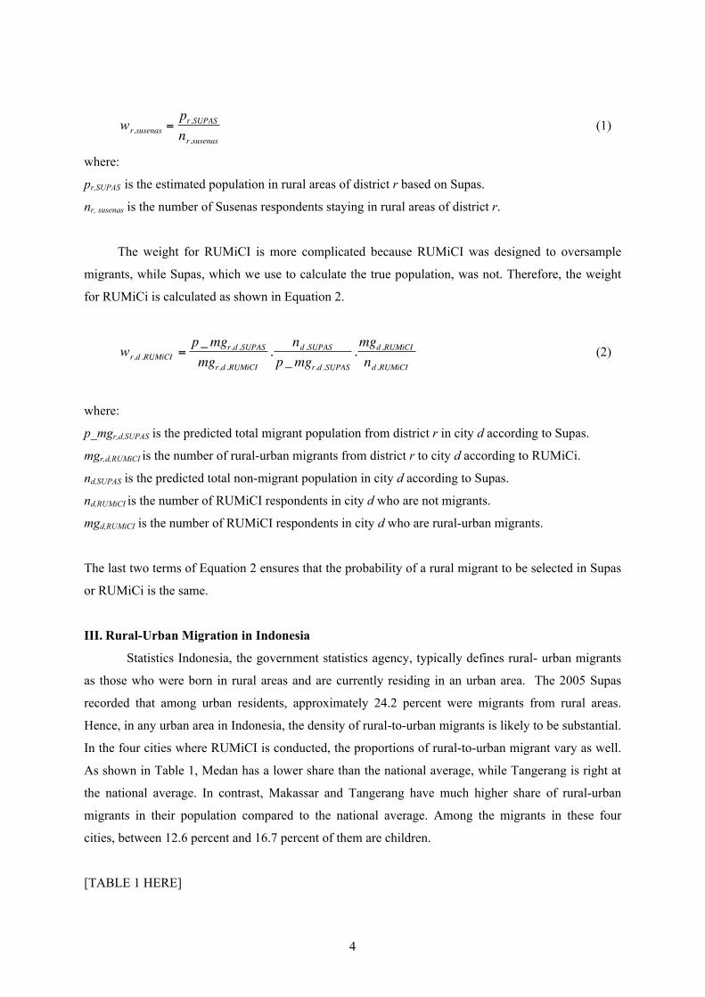
wr,susenas =pr,SUPASnr,susenas
(1)
where:
pr,SUPAS is the estimated population in rural areas of district r based on Supas.
nr, susenas is the number of Susenas respondents staying in rural areas of district r.
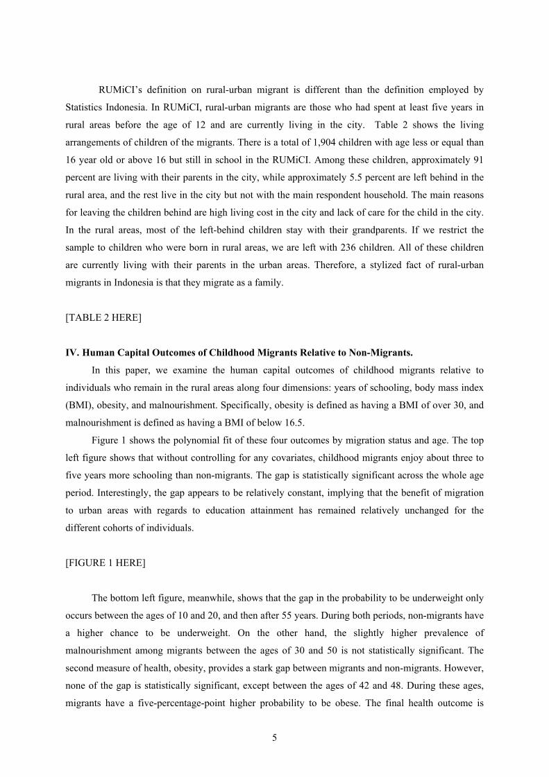
The weight for RUMiCI is more complicated because RUMiCI was designed to oversample
migrants, while Supas, which we use to calculate the true population, was not. Therefore, the weight
for RUMiCi is calculated as shown in Equation 2.
!
wr,d ,RUMiCI =p_mgr,d ,SUPASmgr,d ,RUMiCI
.nd ,SUPAS
p_mgr,d ,SUPAS.mgd ,RUMiCInd ,RUMiCI
(2)
where:
p_mgr,d,SUPAS is the predicted total migrant population from district r in city d according to Supas.
mgr,d,RUMiCI is the number of rural-urban migrants from district r to city d according to RUMiCi.
nd,SUPAS is the predicted total non-migrant population in city d according to Supas.
nd,RUMiCI is the number of RUMiCI respondents in city d who are not migrants.
mgd,RUMiCI is the number of RUMiCI respondents in city d who are rural-urban migrants.
The last two terms of Equation 2 ensures that the probability of a rural migrant to be selected in Supas
or RUMiCi is the same.
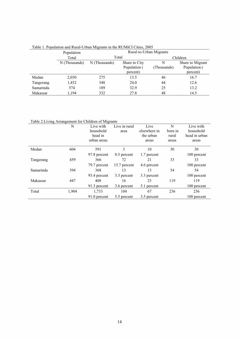
III. Rural-Urban Migration in Indonesia
Statistics Indonesia, the government statistics agency, typically defines rural- urban migrants
as those who were born in rural areas and are currently residing in an urban area. The 2005 Supas
recorded that among urban residents, approximately 24.2 percent were migrants from rural areas.
Hence, in any urban area in Indonesia, the density of rural-to-urban migrants is likely to be substantial.
In the four cities where RUMiCI is conducted, the proportions of rural-to-urban migrant vary as well.
As shown in Table 1, Medan has a lower share than the national average, while Tangerang is right at
the national average. In contrast, Makassar and Tangerang have much higher share of rural-urban
migrants in their population compared to the national average. Among the migrants in these four
cities, between 12.6 percent and 16.7 percent of them are children.
[TABLE 1 HERE]
! 5!
RUMiCI’s definition on rural-urban migrant is different than the definition employed by
Statistics Indonesia. In RUMiCI, rural-urban migrants are those who had spent at least five years in
rural areas before the age of 12 and are currently living in the city. Table 2 shows the living
arrangements of children of the migrants. There is a total of 1,904 children with age less or equal than
16 year old or above 16 but still in school in the RUMiCI. Among these children, approximately 91
percent are living with their parents in the city, while approximately 5.5 percent are left behind in the
rural area, and the rest live in the city but not with the main respondent household. The main reasons
for leaving the children behind are high living cost in the city and lack of care for the child in the city.
In the rural areas, most of the left-behind children stay with their grandparents. If we restrict the
sample to children who were born in rural areas, we are left with 236 children. All of these children
are currently living with their parents in the urban areas. Therefore, a stylized fact of rural-urban
migrants in Indonesia is that they migrate as a family.
[TABLE 2 HERE]
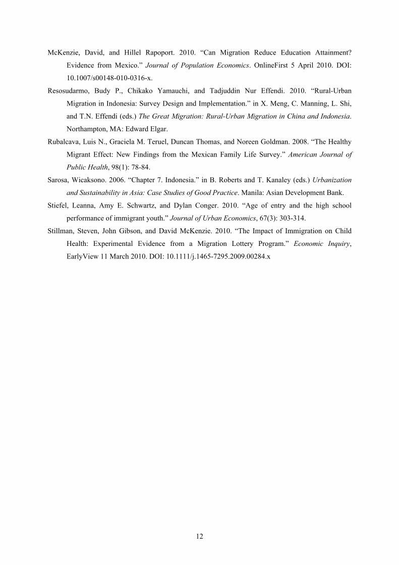
IV. Human Capital Outcomes of Childhood Migrants Relative to Non-Migrants.
In this paper, we examine the human capital outcomes of childhood migrants relative to
individuals who remain in the rural areas along four dimensions: years of schooling, body mass index
(BMI), obesity, and malnourishment. Specifically, obesity is defined as having a BMI of over 30, and
malnourishment is defined as having a BMI of below 16.5.
Figure 1 shows the polynomial fit of these four outcomes by migration status and age. The top
left figure shows that without controlling for any covariates, childhood migrants enjoy about three to
five years more schooling than non-migrants. The gap is statistically significant across the whole age
period. Interestingly, the gap appears to be relatively constant, implying that the benefit of migration
to urban areas with regards to education attainment has remained relatively unchanged for the
different cohorts of individuals.
[FIGURE 1 HERE]
The bottom left figure, meanwhile, shows that the gap in the probability to be underweight only
occurs between the ages of 10 and 20, and then after 55 years. During both periods, non-migrants have
a higher chance to be underweight. On the other hand, the slightly higher prevalence of
malnourishment among migrants between the ages of 30 and 50 is not statistically significant. The
second measure of health, obesity, provides a stark gap between migrants and non-migrants. However,
none of the gap is statistically significant, except between the ages of 42 and 48. During these ages,
migrants have a five-percentage-point higher probability to be obese. The final health outcome is
! 6!
BMI. The bottom right figure shows that 20 to 40-year old migrants and non-migrants have the same
BMI. The difference is that older migrants have significantly higher BMI than similarly aged non-
migrants.
V. Identification Strategy and Estimation Results
The econometric model that we want to estimate is shown in Equation 3.
(3)
where Yij is the education and health outcomes of individual i who were born in rural district j. Our
main explanatory variable is Mij, which is equal to one if the individual followed their parents to the
city and currently live in the city, and is equal to zero if the individual have always lived in the rural
district j. Finally, Xij is a vector of control variables, which contains individual variables such as age,
current marital status, height, and sex; and current household size.
The main difficulty in measuring the effect of migration lies in the fact that migrants are not a
randomly selected group from the population (McKenzie, Gibson, and Stillman, 2010). In addition, in
countries like China, around half of the children of migrants are left behind in the rural areas (Kong
and Meng, 2010). Therefore, the children who migrated with their parents to the city have gone
through two selection processes. This implies that a least squares estimation of Equation 1 is likely to
produce biased coefficients. One cannot consider !M as the effect of childhood migration on an
individual’s current human capital outcomes.
The fact that the share of left-behind children is very low in the Indonesian case implies that in
most cases, rural-urban migrants took their family along when they move to the city. This stylized fact
reduces the estimation difficulty that we need to consider when we estimate the effect of childhood
migration. We only need to worry about one selection process rather than two processes.
Instrument and Estimation Issues
We use the propensity for migration of a rural district as the instrument. The propensity is
calculated by taking the number of migrants from a particular rural district that have migrated to a
particular urban city—in our case, each of the four cities in RUMiCI—and then divide the number by
the number of people currently still residing in the rural district. Since our instrument is calculated at
the district level, our identification relies on the assumption that the variation in the propensity to
migrate across districts is not correlated with the variation in a child’s eventual education and health
outcomes.
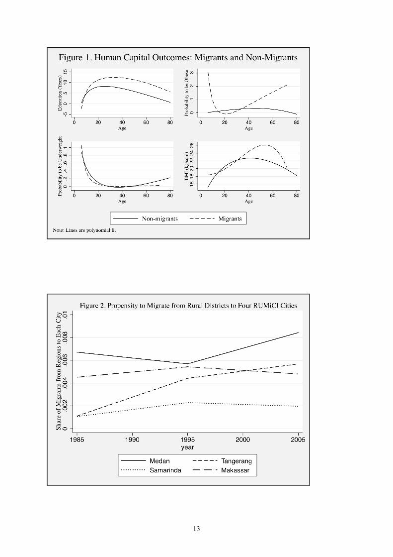
The first issue with the instrument is choosing the year to calculate the propensity for migration.
McKenzie and Rapoport (2010) use historical migration network in their Mexican study. In the
! 7!
Indonesian case, the oldest dataset that we can calculate propensity for migration from is Supas 1985.
In a sense, the choice of a particular year is crucial when the propensity for migration is different over
time. Figure 2 shows the trends in the propensity for migration to the four RUMiCI cities between
1985 and 2005.4 We find no statistically different changes in the migration patterns from rural districts
to Medan and Makassar. In contrast, the propensity to migrate from rural districts to Samarinda
doubled from 0.1 percent to 0.2 percent between 1985 and 1995, and remained constant up to 2005.
The most dramatic increase is migration to Tangerang, which is an industrial city on the outskirts of
Jakarta. The propensity to migrate increased from 0.1 percent in 1985 to 0.4 percent in 1995, although
the increase in the subsequent decade is only 0.1 percentage points. In absolute terms, however, the
increase remained relatively small. This is further corroborated with the fact that the estimation results
remain robust when we use propensity for migration from 1985, 1995, 2005, or all three periods.
Therefore, in our main results we use the propensity for migration in 2005 as the instrument.5
[FIGURE 2 HERE]
Despite trying our best to ensure the validity of our instrument, as discussed in the paragraphs
below, we admit that the instrument is less than ideal. Our preference is to have an instrument at the
household level, which provides a much cleaner identification than a district-level instrument.
Comparing our instrument with others used in the literature, ours is closer to the one used by
McKenzie and Rapoport (2010). However, we could find no other instrument in the Indonesian
context. In addition, we believe that as a first step in understanding the externality of migration in
Indonesia, our instrumental variables estimation still provides a more precise approximation compared
to OLS results.
Given the fact that our instrument is at the district level, we now identify several factors that
could result in our instrument violating the exclusion restriction. A particular issue is related to the fact
that the higher propensity for migration may indicate the existence of a network in the city that
facilitates both the migration and the adaptation process in the city. Since the size of the network in the
city can directly affect the outcomes, the estimated results will be biased upwards. In order to allay
this potential source of bias, we include controls for network size in the city. Specifically, the variable
is calculated as the percentage share of former rural residents of a district who are currently residing in
a city to the total city population. We calculate the network size of each rural district in each of the
four cities surveyed in RUMiCI using Supas 2005.
The second issue that may be related to the higher propensity for migration is the level of
economic development of a rural district, which could also directly human capital accumulation. To
!!!!!!!!!!!!!!!!!!!!!!!!!!!!!!!!!!!!!!!!!!!!!!!!!!!!!!!!4 The migration patterns are calculated using Supas 1985, 1995, and 2005. 5 The estimation results using propensity for migration from 1985, 1995, and all three periods are in the Appendix.
! 8!
control for this as much as possible, we include additional controls to our model, such as island of
birth fixed effects, to further ensure that the districts that we compare from are comparatively similar.
In addition, we control for remoteness and access to health and education facilities at the village where
the residents were born in. We also include a measure of education attainment of the previous
generation in our samples’ district of birth in order to absorb unobserved heterogeneity further.
Ideally, we want to use the education attainment of the parents of each individual in our sample.
However, we have no such data. Since the average age of our sample is 31, we define the previous
generation as those 55 years old or older.
The final issue is related to failed migrants, those families who had tried migrating to the city
but had to return to the rural areas because they could not succeed in the city. How the children of the
failed migrants affect the estimation in this paper is unclear. On one hand, these children—who are
now adults—can be less successful than the children of the permanent rural-urban migrants had they
remained in the city. Therefore, the estimated effect would be overestimated. On the other hand, these
children were actually ‘treated’ for a limited period of time while they were in the city. If the limited
amount of time that they were exposed to education and health services in the city has a permanent
effect, then these children would increase the average education in the rural district. As such, the
estimated effect would be underestimated.
To our knowledge, there is no published information on the extent of migration failures in
Indonesia. We use Supas 1985, 1995, and 2005 to estimate the migration failure rate. Supas records
three sets of information on an individual’s residence: region of birth, region of residence five years
prior to the survey, and current region of residence. From these three sets of information, we create a
set of individuals who were born in a rural area and were living in an urban area five years prior to a
Supas. This is the set of rural-urban migrants. We then classify these individuals based on their current
region of residence. Those still living in urban areas are considered as successful migrants, while those
whose current residence is in rural areas are considered as failed migrants.
Using the algorithm above, we find migration failure rates to be in 9 percent in 1985, 17 percent
in 1995, and 12 percent in 2005. These rates are relatively small, indicating that the vast majority of
rural-urban migrants are successful. Hence, although we cannot completely remove the potential bias,
the potential for the failed migrants to bias our estimations is relatively small and we believe our
estimation results are still reasonable.
With the instrumental variable approach, the first stage of the model is Equation 4 and the
second stage is Equation 5.
(4)
(5)
! 9!
where Rj is the excluded variable, "k is the island of birth fixed effects, and the other variables are the
same as in Equation 3.
Estimation Results
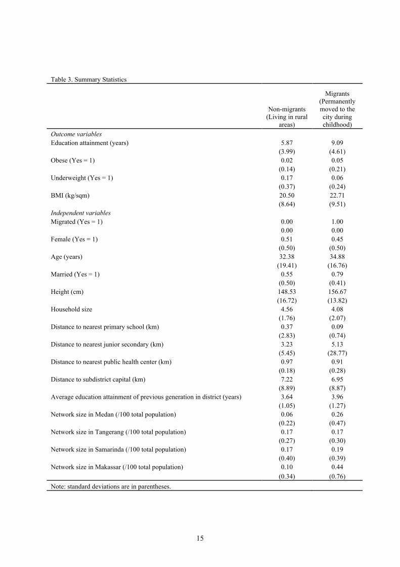
Table 3 contains the summary statistics of the outcomes and the explanatory variables. We
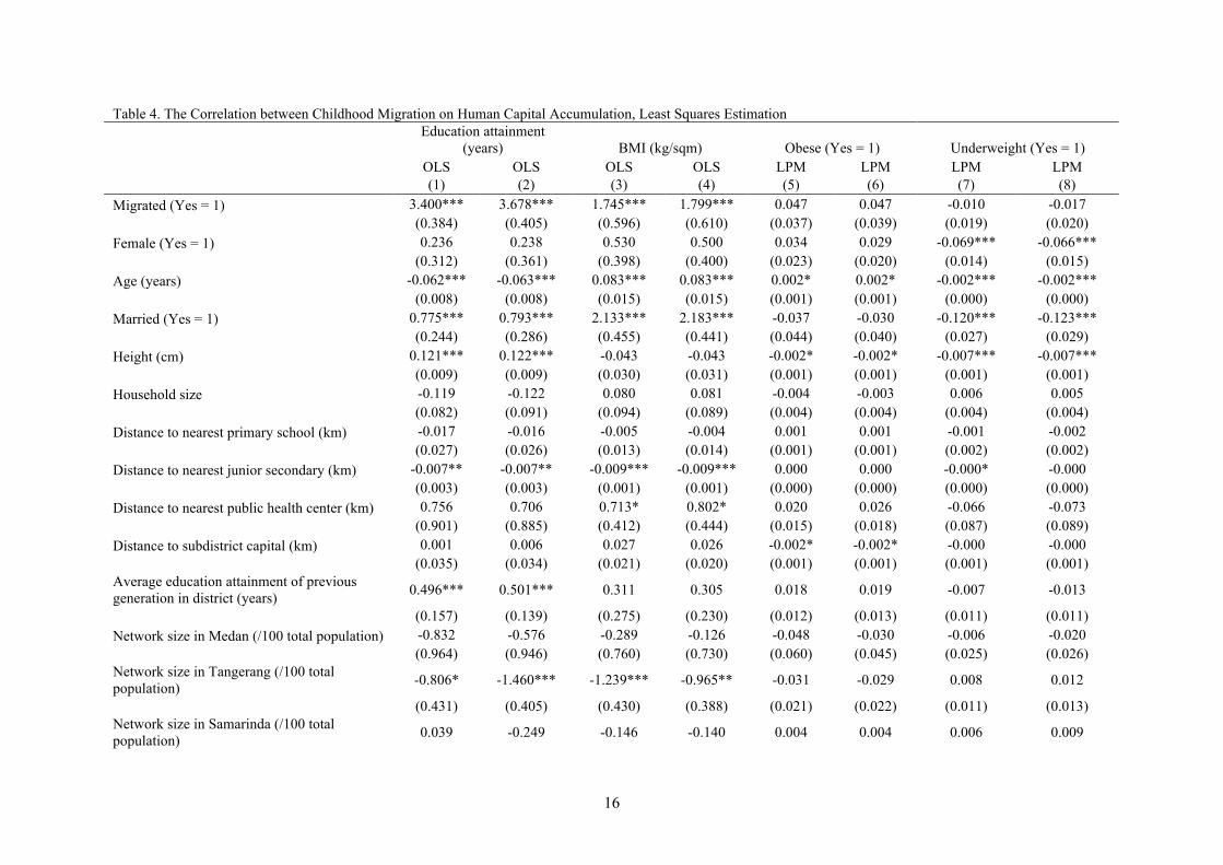
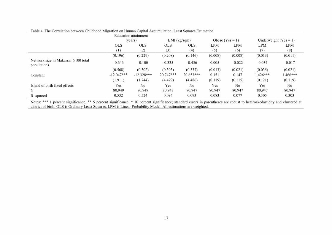
show the OLS results of Equation 3, with and without the island of birth fixed effects, in Table 4. The
table shows that migration is associated with between 3.4 (Column 1) and 3.7 (Column 2) more years
of schooling compared to staying in the rural area. Meanwhile, there is no significant relationship
between migration and obesity, although there is a significant and small relationship between
migration and lower malnourishment. Those who migrated as a child are about 0.1 percentage points
less likely to be underweight than rural residents. Finally, individuals who moved to the city as
children have a higher BMI score by 1.8 kilograms/square meters. Given the results for obesity and
underweight, the BMI results indicate that those who migrated as children are healthier.
[TABLE 3 HERE]
[TABLE 4 HERE]
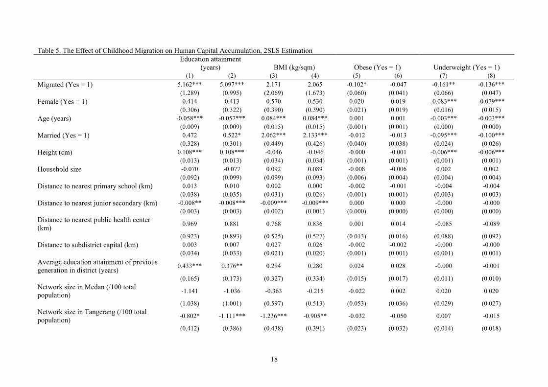
The instrumental variable estimation results are shown in Table 5. The instrument performs
strongly, with the first stage regressions showing statistically significant F-statistics. From the first two
columns, the effect of migration on education attainment is around 5.1 years of additional schooling in
the long-term. In a country where most of the adults only have about nine years of education, this
effect is very large. The effect of migration with regards to obesity is imprecisely estimated. However,
we can rule out any large detrimental effect of childhood migration on adult obesity. More
importantly, however, is the dramatic effect of migration on malnourishment. Childhood migration
lowers the probability to be underweight by around 14 to 16 percentage points. The health results
imply that migration to an urban area during childhood reduces the probability of experiencing
extreme health conditions such as malnourishment, and is not associated with obesity. In summary,
our findings show that children who followed their migrant parents to the city enjoy a large benefit
with regards to education attainment. In addition, they have better health compared to those staying in
the rural districts.
[TABLE 5 HERE]
What are the possible mechanisms that may explain our findings of a positive effect of
childhood migration on education and health? As we mention in the introduction, these mechanisms
! 10!
may include differences in the availability of health and education facilities between urban and rural
areas or the higher returns to education and health investments in urban areas. We discuss these two
aspects in turn.
In Indonesia, inequality in the availability of health and education facilities between urban and
rural areas is large. In a review paper, Darja et al (2005) find that as late as in 1999, only 30 percent of
rural villages in Indonesia had a junior secondary school (grades seven to nine), while about 9 percent
had a public senior secondary school (grades 10 to 12). In contrast, 88 percent of urban villages had a
junior secondary school, and 64 percent had a senior secondary school. Given that the average age of
our sample is 33 years, secondary school availability in rural areas must have been even worse in late
1980s, the time our sample was at secondary school age. However, the difference in the availability of
health facilities between urban and rural areas is not as large. In the same paper, Darja et al (2005) find
that in 1999, about 37 percent of rural villages had a public health center, compared to 52 percent of
urban villages. Although it is true that there was practically no hospital in rural areas, the public health
centers are the main provider of healthcare in Indonesia. Therefore, the relatively smaller gap in the
access to these centers may explain the relatively small effect of migrating to urban areas on health
outcomes.
The second mechanism that could explain the higher education attainment of childhood
migrants compared to those who remained in the rural area pertains to the returns to investment in
education. Assuming a perfect access to credit market, a parent would continue to invest in their
children’s schooling if the net returns to additional schooling are larger than the net returns to an
alternative investment. Based on this concept, it appears that the net returns to investment in education
becomes smaller than the returns to an alternative investment at quite an early stage of education in
rural areas, but happens much later in urban areas. However, empirically testing this hypothesis would
entail measuring the net returns to all alternative investment choices, including a child’s education.
We know of no such dataset in Indonesia that would allow us to empirically test this conjecture.
Perhaps for this reason, we find almost no empirical research on this issue in the literature.6
VI. Conclusion
Developing countries are experiencing unprecedented levels of urbanization. Although most of
these movements are motivated by economic reasons, it is possible that they affect the human capital
accumulation of the children who follow their parents to the cities. Assessing this externality is
important, because if it turns out to be negative, government intervention may be required. This paper
!!!!!!!!!!!!!!!!!!!!!!!!!!!!!!!!!!!!!!!!!!!!!!!!!!!!!!!!6 Note that merely comparing the returns to education in urban and rural areas separately is not adequate for this purpose. Establishing higher returns to education in urban areas compared to rural areas is not a sufficient explanation, because when the decision whether to invest in additional schooling for the child is taken, a decision maker is comparing the returns of the investment to returns of alternative investments in the area where he or she resides, not in other areas.
! 11!
estimates the effect of permanently migrating as a child from a rural area to an urban area on human
capital outcomes. Despite weaknesses in our instrument, we believe that our results still provide a
reasonable first approximation of the effect of childhood migration. In the context of Indonesia, this
study is the first step in what is an increasingly important area of research as the country continues to
urbanize.
We utilize a recent survey of urban-rural migrants in Indonesia, the RUMiCI, and merge it with
the national socioeconomic survey to create a dataset that contains the migrants in urban areas and
non-migrants in rural areas who were born in the same rural districts. We employ a measure of
district-level propensity to migrate, calculated from the intercensal surveys, as an instrument.
To summarize the findings, we find childhood migration to urban areas increased education
attainment by around five years of schooling relative to an observably similar individual who
remained in the rural area. In addition, the childhood migrants are significantly healthier, facing a
lower probability to be underweight by about 17 percentage points. Therefore, our findings indicate
the existence of a positive externality of migrating from rural to urban areas on the children of the
migrants.
There are many channels through which migration could affect an individual’s human capital
outcomes. These include increased food intake, improved health practices, higher access to quality
education and health facilities, higher labor market returns to education and health, or peer effects.
However, we do not have sufficient information to determine which channel is dominant. Therefore,
we leave the investigation into potential channels for future studies.
References
Darja, Jesse, Daniel Suryadarma, Asep Suryahadi, and Sudarno Sumarto. 2005. “What Happened to
Village Infrastructure and Public Services during the Economic Crisis in Indonesia?”
Economics and Finance in Indonesia, 53(2): 119-145.
Frijters, Paul and Xin Meng. 2009. Rural to Urban Migration in China: An Overview. mimeo.
Australian National University.
Gang, Ira N. and Klaus F. Zimmermann. 2000. “Is Child like Parent? Educational Attainment and
Ethnic Origin.” Journal of Human Resources, 35(3): 550-569.
Kong, Sherry Tao and Xin Meng. 2010. “The Educational and Health Outcomes of the Children of
Migrants.” in X. Meng, C. Manning, L. Shi, and T.N. Effendi (eds.) The Great Migration:
Rural-Urban Migration in China and Indonesia. Northampton, MA: Edward Elgar.
Liang, Zai and Yiu Por Chen. 2007. “The educational consequences of migration for children in
China.” Social Science Research, 36(1): 28-47.
McKenzie, David, John Gibson, and Steven Stillman. 2010. “How Important is Selection?
Experimental vs Non-experimental Measures of the Income Gains from Migration.” Journal of
the European Economic Association, 8(4): 913-945.
! 12!
McKenzie, David, and Hillel Rapoport. 2010. “Can Migration Reduce Education Attainment?
Evidence from Mexico.” Journal of Population Economics. OnlineFirst 5 April 2010. DOI:
10.1007/s00148-010-0316-x.
Resosudarmo, Budy P., Chikako Yamauchi, and Tadjuddin Nur Effendi. 2010. “Rural-Urban
Migration in Indonesia: Survey Design and Implementation.” in X. Meng, C. Manning, L. Shi,
and T.N. Effendi (eds.) The Great Migration: Rural-Urban Migration in China and Indonesia.
Northampton, MA: Edward Elgar.
Rubalcava, Luis N., Graciela M. Teruel, Duncan Thomas, and Noreen Goldman. 2008. “The Healthy
Migrant Effect: New Findings from the Mexican Family Life Survey.” American Journal of
Public Health, 98(1): 78-84.
Sarosa, Wicaksono. 2006. “Chapter 7. Indonesia.” in B. Roberts and T. Kanaley (eds.) Urbanization
and Sustainability in Asia: Case Studies of Good Practice. Manila: Asian Development Bank.
Stiefel, Leanna, Amy E. Schwartz, and Dylan Conger. 2010. “Age of entry and the high school
performance of immigrant youth.” Journal of Urban Economics, 67(3): 303-314.
Stillman, Steven, John Gibson, and David McKenzie. 2010. “The Impact of Immigration on Child
Health: Experimental Evidence from a Migration Lottery Program.” Economic Inquiry,
EarlyView 11 March 2010. DOI: 10.1111/j.1465-7295.2009.00284.x
! 13!
! 14!
Table 1. Population and Rural-Urban Migrants in the RUMiCI Cities, 2005 Population Rural-to-Urban Migrants Total Total Children
N (Thousands) N (Thousands) Share to City Population (
percent)
N (Thousands)
Share to Migrant Population (
percent) Medan 2,030 275 13.5 46 16.7 Tangerang 1,452 348 24.0 44 12.6 Samarinda 574 189 32.9 25 13.2 Makassar 1,194 332 27.8 48 14.5
Table 2.Living Arrangement for Children of Migrants
N Live with household
head in urban areas
Live in rural area
Live elsewhere in
the urban areas
N born in
rural areas
Live with household
head in urban areas
Medan 604 591 3 10 30 30 97.8 percent 0.5 percent 1.7 percent 100 percent Tangerang 459 366 72 21 33 33 79.7 percent 15.7 percent 4.6 percent 100 percent Samarinda 394 368 13 13 54 54 93.4 percent 3.3 percent 3.3 percent 100 percent Makassar 447 408 16 23 119 119 91.3 percent 3.6 percent 5.1 percent 100 percent Total 1,904 1,733 104 67 236 236 91.0 percent 5.5 percent 3.5 percent 100 percent
! 15!
Table 3. Summary Statistics
Non-migrants (Living in rural
areas)
Migrants (Permanently moved to the city during childhood)
Outcome variables Education attainment (years) 5.87 9.09 (3.99) (4.61) Obese (Yes = 1) 0.02 0.05 (0.14) (0.21) Underweight (Yes = 1) 0.17 0.06 (0.37) (0.24) BMI (kg/sqm) 20.50 22.71 (8.64) (9.51) Independent variables Migrated (Yes = 1) 0.00 1.00 0.00 0.00 Female (Yes = 1) 0.51 0.45 (0.50) (0.50) Age (years) 32.38 34.88 (19.41) (16.76) Married (Yes = 1) 0.55 0.79 (0.50) (0.41) Height (cm) 148.53 156.67 (16.72) (13.82) Household size 4.56 4.08 (1.76) (2.07) Distance to nearest primary school (km) 0.37 0.09 (2.83) (0.74) Distance to nearest junior secondary (km) 3.23 5.13 (5.45) (28.77) Distance to nearest public health center (km) 0.97 0.91 (0.18) (0.28) Distance to subdistrict capital (km) 7.22 6.95 (8.89) (8.87) Average education attainment of previous generation in district (years) 3.64 3.96 (1.05) (1.27) Network size in Medan (/100 total population) 0.06 0.26 (0.22) (0.47) Network size in Tangerang (/100 total population) 0.17 0.17 (0.27) (0.30) Network size in Samarinda (/100 total population) 0.17 0.19 (0.40) (0.39) Network size in Makassar (/100 total population) 0.10 0.44 (0.34) (0.76) Note: standard deviations are in parentheses.
! 16!
Table 4. The Correlation between Childhood Migration on Human Capital Accumulation, Least Squares Estimation
Education attainment
(years) BMI (kg/sqm) Obese (Yes = 1) Underweight (Yes = 1) OLS OLS OLS OLS LPM LPM LPM LPM (1) (2) (3) (4) (5) (6) (7) (8) Migrated (Yes = 1) 3.400*** 3.678*** 1.745*** 1.799*** 0.047 0.047 -0.010 -0.017 (0.384) (0.405) (0.596) (0.610) (0.037) (0.039) (0.019) (0.020) Female (Yes = 1) 0.236 0.238 0.530 0.500 0.034 0.029 -0.069*** -0.066*** (0.312) (0.361) (0.398) (0.400) (0.023) (0.020) (0.014) (0.015) Age (years) -0.062*** -0.063*** 0.083*** 0.083*** 0.002* 0.002* -0.002*** -0.002*** (0.008) (0.008) (0.015) (0.015) (0.001) (0.001) (0.000) (0.000) Married (Yes = 1) 0.775*** 0.793*** 2.133*** 2.183*** -0.037 -0.030 -0.120*** -0.123*** (0.244) (0.286) (0.455) (0.441) (0.044) (0.040) (0.027) (0.029) Height (cm) 0.121*** 0.122*** -0.043 -0.043 -0.002* -0.002* -0.007*** -0.007*** (0.009) (0.009) (0.030) (0.031) (0.001) (0.001) (0.001) (0.001) Household size -0.119 -0.122 0.080 0.081 -0.004 -0.003 0.006 0.005 (0.082) (0.091) (0.094) (0.089) (0.004) (0.004) (0.004) (0.004) Distance to nearest primary school (km) -0.017 -0.016 -0.005 -0.004 0.001 0.001 -0.001 -0.002 (0.027) (0.026) (0.013) (0.014) (0.001) (0.001) (0.002) (0.002) Distance to nearest junior secondary (km) -0.007** -0.007** -0.009*** -0.009*** 0.000 0.000 -0.000* -0.000 (0.003) (0.003) (0.001) (0.001) (0.000) (0.000) (0.000) (0.000) Distance to nearest public health center (km) 0.756 0.706 0.713* 0.802* 0.020 0.026 -0.066 -0.073 (0.901) (0.885) (0.412) (0.444) (0.015) (0.018) (0.087) (0.089) Distance to subdistrict capital (km) 0.001 0.006 0.027 0.026 -0.002* -0.002* -0.000 -0.000 (0.035) (0.034) (0.021) (0.020) (0.001) (0.001) (0.001) (0.001) Average education attainment of previous generation in district (years) 0.496*** 0.501*** 0.311 0.305 0.018 0.019 -0.007 -0.013
(0.157) (0.139) (0.275) (0.230) (0.012) (0.013) (0.011) (0.011) Network size in Medan (/100 total population) -0.832 -0.576 -0.289 -0.126 -0.048 -0.030 -0.006 -0.020 (0.964) (0.946) (0.760) (0.730) (0.060) (0.045) (0.025) (0.026) Network size in Tangerang (/100 total population) -0.806* -1.460*** -1.239*** -0.965** -0.031 -0.029 0.008 0.012
(0.431) (0.405) (0.430) (0.388) (0.021) (0.022) (0.011) (0.013) Network size in Samarinda (/100 total population) 0.039 -0.249 -0.146 -0.140 0.004 0.004 0.006 0.009
! 17!
Table 4. The Correlation between Childhood Migration on Human Capital Accumulation, Least Squares Estimation
Education attainment
(years) BMI (kg/sqm) Obese (Yes = 1) Underweight (Yes = 1) OLS OLS OLS OLS LPM LPM LPM LPM (1) (2) (3) (4) (5) (6) (7) (8) (0.196) (0.229) (0.208) (0.146) (0.008) (0.008) (0.013) (0.011) Network size in Makassar (/100 total population) -0.646 -0.100 -0.335 -0.456 0.005 -0.022 -0.034 -0.017
(0.568) (0.302) (0.303) (0.337) (0.013) (0.021) (0.035) (0.021) Constant -12.047*** -12.328*** 20.747*** 20.653*** 0.151 0.147 1.426*** 1.466*** (1.911) (1.744) (4.479) (4.486) (0.119) (0.115) (0.121) (0.119) Island of birth fixed effects Yes No Yes No Yes No Yes No N 80,949 80,949 80,947 80,947 80,947 80,947 80,947 80,947 R-squared 0.532 0.524 0.094 0.093 0.083 0.077 0.305 0.303
Notes: *** 1 percent significance, ** 5 percent significance, * 10 percent significance; standard errors in parentheses are robust to heteroskedasticity and clustered at district of birth; OLS is Ordinary Least Squares, LPM is Linear Probability Model. All estimations are weighted.
! 18!
Table 5. The Effect of Childhood Migration on Human Capital Accumulation, 2SLS Estimation
Education attainment
(years) BMI (kg/sqm) Obese (Yes = 1) Underweight (Yes = 1) (1) (2) (3) (4) (5) (6) (7) (8) Migrated (Yes = 1) 5.162*** 5.097*** 2.171 2.065 -0.102* -0.047 -0.161** -0.136*** (1.289) (0.995) (2.069) (1.673) (0.060) (0.041) (0.066) (0.047) Female (Yes = 1) 0.414 0.413 0.570 0.530 0.020 0.019 -0.083*** -0.079*** (0.306) (0.322) (0.390) (0.390) (0.021) (0.019) (0.016) (0.015) Age (years) -0.058*** -0.057*** 0.084*** 0.084*** 0.001 0.001 -0.003*** -0.003*** (0.009) (0.009) (0.015) (0.015) (0.001) (0.001) (0.000) (0.000) Married (Yes = 1) 0.472 0.522* 2.062*** 2.133*** -0.012 -0.013 -0.095*** -0.100*** (0.328) (0.301) (0.449) (0.426) (0.040) (0.038) (0.024) (0.026) Height (cm) 0.108*** 0.108*** -0.046 -0.046 -0.000 -0.001 -0.006*** -0.006*** (0.013) (0.013) (0.034) (0.034) (0.001) (0.001) (0.001) (0.001) Household size -0.070 -0.077 0.092 0.089 -0.008 -0.006 0.002 0.002 (0.092) (0.099) (0.099) (0.093) (0.006) (0.004) (0.004) (0.004) Distance to nearest primary school (km) 0.013 0.010 0.002 0.000 -0.002 -0.001 -0.004 -0.004 (0.038) (0.035) (0.031) (0.026) (0.001) (0.001) (0.003) (0.003) Distance to nearest junior secondary (km) -0.008** -0.008*** -0.009*** -0.009*** 0.000 0.000 -0.000 -0.000 (0.003) (0.003) (0.002) (0.001) (0.000) (0.000) (0.000) (0.000) Distance to nearest public health center (km) 0.969 0.881 0.768 0.836 0.001 0.014 -0.085 -0.089
(0.923) (0.893) (0.525) (0.527) (0.013) (0.016) (0.088) (0.092) Distance to subdistrict capital (km) 0.003 0.007 0.027 0.026 -0.002 -0.002 -0.000 -0.000 (0.034) (0.033) (0.021) (0.020) (0.001) (0.001) (0.001) (0.001) Average education attainment of previous generation in district (years) 0.433*** 0.376** 0.294 0.280 0.024 0.028 -0.000 -0.001
(0.165) (0.173) (0.327) (0.334) (0.015) (0.017) (0.011) (0.010) Network size in Medan (/100 total population) -1.141 -1.036 -0.363 -0.215 -0.022 0.002 0.020 0.020
(1.038) (1.001) (0.597) (0.513) (0.053) (0.036) (0.029) (0.027) Network size in Tangerang (/100 total population) -0.802* -1.111*** -1.236*** -0.905** -0.032 -0.050 0.007 -0.015
(0.412) (0.386) (0.438) (0.391) (0.023) (0.032) (0.014) (0.018)
! 19!
Table 5. The Effect of Childhood Migration on Human Capital Accumulation, 2SLS Estimation
Education attainment
(years) BMI (kg/sqm) Obese (Yes = 1) Underweight (Yes = 1) (1) (2) (3) (4) (5) (6) (7) (8) Network size in Samarinda (/100 total population) 0.103 0.036 -0.127 -0.087 -0.003 -0.015 -0.001 -0.015
(0.206) (0.254) (0.226) (0.292) (0.010) (0.015) (0.010) (0.009) Network size in Makassar (/100 total population) -0.761 -0.491 -0.375 -0.531 0.020 0.005 -0.020 0.016
(0.539) (0.368) (0.387) (0.590) (0.015) (0.018) (0.030) (0.014) Constant -11.166*** -10.917*** 21.009*** 20.935*** 0.104 0.047 1.347*** 1.339*** (1.868) (1.834) (4.663) (4.898) (0.133) (0.137) (0.119) (0.126) Island of birth fixed effects Yes No Yes No Yes No Yes No N 80,949 80,949 80,947 80,947 80,947 80,947 80,947 80,947 R-squared 0.514 0.510 0.093 0.092 -0.016 0.031 0.271 0.278 First stage F-stat 14.12 23.64 15.85 27.88 15.85 27.88 15.85 27.88 Notes: *** 1 percent significance, ** 5 percent significance, * 10 percent significance; standard errors in parentheses are robust to heteroskedasticity and clustered at district of birth; instrument used in 2SLS estimations are the number of migrants from a rural district who are living in each of the four cities divided by the number of population in the rural district in 2005. All estimations are weighted.
! 20!
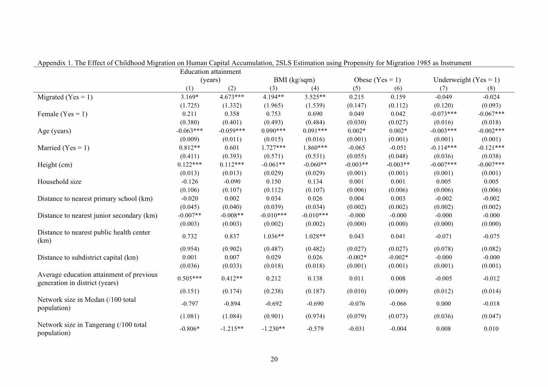
Appendix 1. The Effect of Childhood Migration on Human Capital Accumulation, 2SLS Estimation using Propensity for Migration 1985 as Instrument
Education attainment
(years) BMI (kg/sqm) Obese (Yes = 1) Underweight (Yes = 1) (1) (2) (3) (4) (5) (6) (7) (8) Migrated (Yes = 1) 3.169* 4.673*** 4.194** 3.525** 0.215 0.159 -0.049 -0.024 (1.725) (1.332) (1.965) (1.539) (0.147) (0.112) (0.120) (0.093) Female (Yes = 1) 0.211 0.358 0.753 0.690 0.049 0.042 -0.073*** -0.067*** (0.380) (0.401) (0.493) (0.484) (0.030) (0.027) (0.016) (0.018) Age (years) -0.063*** -0.059*** 0.090*** 0.091*** 0.002* 0.002* -0.003*** -0.002*** (0.009) (0.011) (0.015) (0.016) (0.001) (0.001) (0.001) (0.001) Married (Yes = 1) 0.812** 0.601 1.727*** 1.860*** -0.065 -0.051 -0.114*** -0.121*** (0.411) (0.393) (0.571) (0.531) (0.055) (0.048) (0.036) (0.038) Height (cm) 0.122*** 0.112*** -0.061** -0.060** -0.003** -0.003** -0.007*** -0.007*** (0.013) (0.013) (0.029) (0.029) (0.001) (0.001) (0.001) (0.001) Household size -0.126 -0.090 0.150 0.134 0.001 0.001 0.005 0.005 (0.106) (0.107) (0.112) (0.107) (0.006) (0.006) (0.006) (0.006) Distance to nearest primary school (km) -0.020 0.002 0.034 0.026 0.004 0.003 -0.002 -0.002 (0.045) (0.040) (0.039) (0.034) (0.002) (0.002) (0.002) (0.002) Distance to nearest junior secondary (km) -0.007** -0.008** -0.010*** -0.010*** -0.000 -0.000 -0.000 -0.000 (0.003) (0.003) (0.002) (0.002) (0.000) (0.000) (0.000) (0.000) Distance to nearest public health center (km) 0.732 0.837 1.036** 1.028** 0.043 0.041 -0.071 -0.075
(0.954) (0.902) (0.487) (0.482) (0.027) (0.027) (0.078) (0.082) Distance to subdistrict capital (km) 0.001 0.007 0.029 0.026 -0.002* -0.002* -0.000 -0.000 (0.036) (0.033) (0.018) (0.018) (0.001) (0.001) (0.001) (0.001) Average education attainment of previous generation in district (years) 0.505*** 0.412** 0.212 0.138 0.011 0.008 -0.005 -0.012
(0.151) (0.174) (0.238) (0.187) (0.010) (0.009) (0.012) (0.014) Network size in Medan (/100 total population) -0.797 -0.894 -0.692 -0.690 -0.076 -0.066 0.000 -0.018
(1.081) (1.084) (0.901) (0.974) (0.079) (0.073) (0.036) (0.047) Network size in Tangerang (/100 total population) -0.806* -1.215** -1.230** -0.579 -0.031 -0.004 0.008 0.010
! 21!
Appendix 1. The Effect of Childhood Migration on Human Capital Accumulation, 2SLS Estimation using Propensity for Migration 1985 as Instrument
Education attainment
(years) BMI (kg/sqm) Obese (Yes = 1) Underweight (Yes = 1) (1) (2) (3) (4) (5) (6) (7) (8) (0.436) (0.496) (0.516) (0.535) (0.025) (0.023) (0.011) (0.024) Network size in Samarinda (/100 total population) 0.030 -0.049 -0.038 0.205 0.011 0.026 0.004 0.008
(0.197) (0.291) (0.213) (0.313) (0.011) (0.018) (0.012) (0.017) Network size in Makassar (/100 total population) -0.631 -0.373 -0.569 -0.937* -0.011 -0.053 -0.030 -0.015
(0.553) (0.387) (0.383) (0.489) (0.022) (0.038) (0.037) (0.028) Constant -11.897*** -11.335*** 21.846*** 22.512*** 0.233* 0.265* 1.392*** 1.457*** (1.909) (1.712) (3.869) (3.889) (0.141) (0.139) (0.136) (0.164) Island of birth fixed effects Yes No Yes No Yes No Yes No N 80,632 80,632 80,630 80,630 80,630 80,630 80,630 80,630 R-squared 0.532 0.517 0.078 0.083 -0.043 0.013 0.303 0.302 First stage F-stat 11.533 17.510 13.878 18.006 13.878 18.006 13.878 18.006 Notes: *** 1 percent significance, ** 5 percent significance, * 10 percent significance; standard errors in parentheses are robust to heteroskedasticity and clustered at district of birth; instrument used in 2SLS estimations are the number of migrants from a rural district who are living in each of the four cities divided by the number of population in the rural district. All estimations are weighted.
! 22!
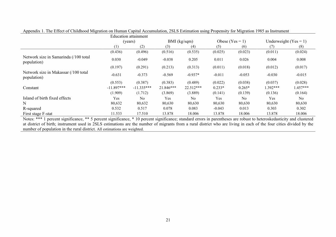
Appendix 2. The Effect of Childhood Migration on Human Capital Accumulation, 2SLS Estimation using Propensity for Migration 1995 as Instrument
Education attainment
(years) BMI (kg/sqm) Obese (Yes = 1) Underweight (Yes = 1) (1) (2) (3) (4) (5) (6) (7) (8) Migrated (Yes = 1) 3.900** 4.922*** 5.327*** 4.660*** 0.287 0.233 -0.191* -0.083 (1.839) (1.617) (1.841) (1.670) (0.199) (0.163) (0.101) (0.080) Female (Yes = 1) 0.287 0.391 0.864* 0.821 0.056 0.050 -0.086*** -0.073*** (0.396) (0.454) (0.494) (0.518) (0.036) (0.035) (0.017) (0.017) Age (years) -0.061*** -0.058*** 0.093*** 0.095*** 0.003* 0.003* -0.003*** -0.003*** (0.009) (0.011) (0.015) (0.017) (0.001) (0.002) (0.001) (0.001) Married (Yes = 1) 0.689* 0.556 1.534** 1.645*** -0.077 -0.065 -0.090*** -0.110*** (0.413) (0.450) (0.604) (0.609) (0.065) (0.059) (0.025) (0.033) Height (cm) 0.117*** 0.110*** -0.069** -0.071** -0.003* -0.003* -0.006*** -0.006*** (0.014) (0.015) (0.029) (0.030) (0.002) (0.002) (0.001) (0.001) Household size -0.105 -0.082 0.182* 0.168 0.003 0.003 0.001 0.003 (0.095) (0.092) (0.103) (0.105) (0.007) (0.006) (0.005) (0.005) Distance to nearest primary school (km) -0.008 0.007 0.055 0.048 0.005 0.004 -0.004 -0.003 (0.051) (0.047) (0.036) (0.035) (0.003) (0.003) (0.003) (0.002) Distance to nearest junior secondary (km) -0.007** -0.008** -0.011*** -0.011*** -0.000 -0.000 -0.000 -0.000 (0.003) (0.003) (0.002) (0.002) (0.000) (0.000) (0.000) (0.000) Distance to nearest public health center (km) 0.816 0.859 1.175** 1.169** 0.051 0.050 -0.089 -0.082
(1.001) (0.943) (0.514) (0.520) (0.033) (0.034) (0.087) (0.086) Distance to subdistrict capital (km) 0.002 0.007 0.030* 0.027 -0.002* -0.002* -0.000 -0.000 (0.035) (0.033) (0.018) (0.018) (0.001) (0.001) (0.001) (0.001) Average education attainment of previous generation in district (years) 0.478*** 0.391** 0.168 0.032 0.008 0.001 0.001 -0.006
(0.153) (0.199) (0.278) (0.274) (0.011) (0.012) (0.011) (0.013) Network size in Medan (/100 total population) -0.920 -0.979 -0.910 -1.077 -0.089 -0.091 0.025 0.002
(1.080) (1.131) (0.886) (0.952) (0.087) (0.091) (0.036) (0.041) Network size in Tangerang (/100 total population) -0.805* -1.154** -1.218** -0.325 -0.030 0.012 0.007 -0.003
(0.421) (0.456) (0.575) (0.563) (0.029) (0.030) (0.016) (0.022)
! 23!
Appendix 2. The Effect of Childhood Migration on Human Capital Accumulation, 2SLS Estimation using Propensity for Migration 1995 as Instrument
Education attainment
(years) BMI (kg/sqm) Obese (Yes = 1) Underweight (Yes = 1) (1) (2) (3) (4) (5) (6) (7) (8) Network size in Samarinda (/100 total population) 0.057 0.001 0.012 0.429 0.014 0.041 -0.002 -0.004
(0.192) (0.280) (0.237) (0.365) (0.014) (0.029) (0.010) (0.014) Network size in Makassar (/100 total population) -0.678 -0.442 -0.676 -1.258** -0.017 -0.073 -0.017 0.001
(0.558) (0.435) (0.486) (0.596) (0.029) (0.053) (0.030) (0.022) Constant -11.636*** -11.092*** 22.298*** 23.683*** 0.263 0.343* 1.335*** 1.396*** (1.776) (1.821) (3.882) (4.103) (0.165) (0.191) (0.128) (0.153) Island of birth fixed effects Yes No Yes No Yes No Yes No N 80,949 80,949 80,947 80,947 80,947 80,947 80,947 80,947 R-squared 0.531 0.513 0.059 0.067 -0.174 -0.100 0.256 0.295 First stage F-stat 11.359 12.624 19.545 12.698 19.545 12.698 19.545 12.698 Notes: *** 1 percent significance, ** 5 percent significance, * 10 percent significance; standard errors in parentheses are robust to heteroskedasticity and clustered at district of birth; instrument used in 2SLS estimations are the number of migrants from a rural district who are living in each of the four cities divided by the number of population in the rural district. All estimations are weighted.
! 24!
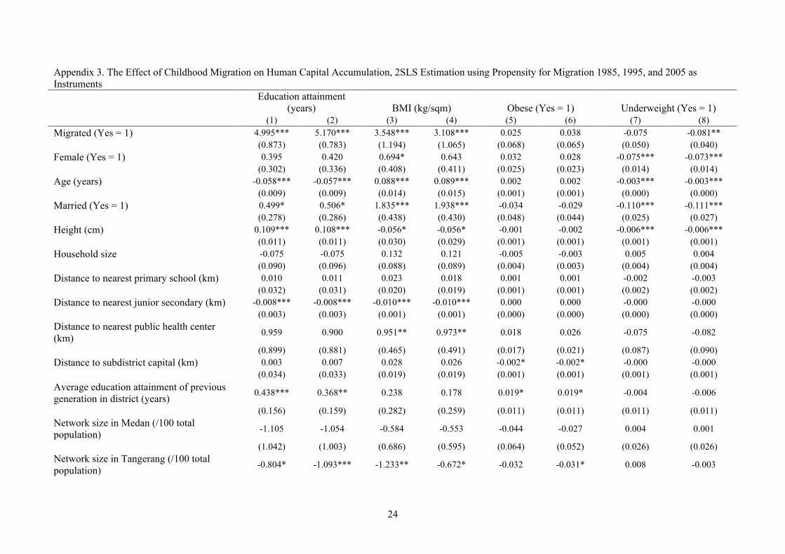
Appendix 3. The Effect of Childhood Migration on Human Capital Accumulation, 2SLS Estimation using Propensity for Migration 1985, 1995, and 2005 as Instruments
Education attainment
(years) BMI (kg/sqm) Obese (Yes = 1) Underweight (Yes = 1) (1) (2) (3) (4) (5) (6) (7) (8) Migrated (Yes = 1) 4.995*** 5.170*** 3.548*** 3.108*** 0.025 0.038 -0.075 -0.081** (0.873) (0.783) (1.194) (1.065) (0.068) (0.065) (0.050) (0.040) Female (Yes = 1) 0.395 0.420 0.694* 0.643 0.032 0.028 -0.075*** -0.073*** (0.302) (0.336) (0.408) (0.411) (0.025) (0.023) (0.014) (0.014) Age (years) -0.058*** -0.057*** 0.088*** 0.089*** 0.002 0.002 -0.003*** -0.003*** (0.009) (0.009) (0.014) (0.015) (0.001) (0.001) (0.000) (0.000) Married (Yes = 1) 0.499* 0.506* 1.835*** 1.938*** -0.034 -0.029 -0.110*** -0.111*** (0.278) (0.286) (0.438) (0.430) (0.048) (0.044) (0.025) (0.027) Height (cm) 0.109*** 0.108*** -0.056* -0.056* -0.001 -0.002 -0.006*** -0.006*** (0.011) (0.011) (0.030) (0.029) (0.001) (0.001) (0.001) (0.001) Household size -0.075 -0.075 0.132 0.121 -0.005 -0.003 0.005 0.004 (0.090) (0.096) (0.088) (0.089) (0.004) (0.003) (0.004) (0.004) Distance to nearest primary school (km) 0.010 0.011 0.023 0.018 0.001 0.001 -0.002 -0.003 (0.032) (0.031) (0.020) (0.019) (0.001) (0.001) (0.002) (0.002) Distance to nearest junior secondary (km) -0.008*** -0.008*** -0.010*** -0.010*** 0.000 0.000 -0.000 -0.000 (0.003) (0.003) (0.001) (0.001) (0.000) (0.000) (0.000) (0.000) Distance to nearest public health center (km) 0.959 0.900 0.951** 0.973** 0.018 0.026 -0.075 -0.082
(0.899) (0.881) (0.465) (0.491) (0.017) (0.021) (0.087) (0.090) Distance to subdistrict capital (km) 0.003 0.007 0.028 0.026 -0.002* -0.002* -0.000 -0.000 (0.034) (0.033) (0.019) (0.019) (0.001) (0.001) (0.001) (0.001) Average education attainment of previous generation in district (years) 0.438*** 0.368** 0.238 0.178 0.019* 0.019* -0.004 -0.006
(0.156) (0.159) (0.282) (0.259) (0.011) (0.011) (0.011) (0.011) Network size in Medan (/100 total population) -1.105 -1.054 -0.584 -0.553 -0.044 -0.027 0.004 0.001
(1.042) (1.003) (0.686) (0.595) (0.064) (0.052) (0.026) (0.026) Network size in Tangerang (/100 total population) -0.804* -1.093*** -1.233** -0.672* -0.032 -0.031* 0.008 -0.003
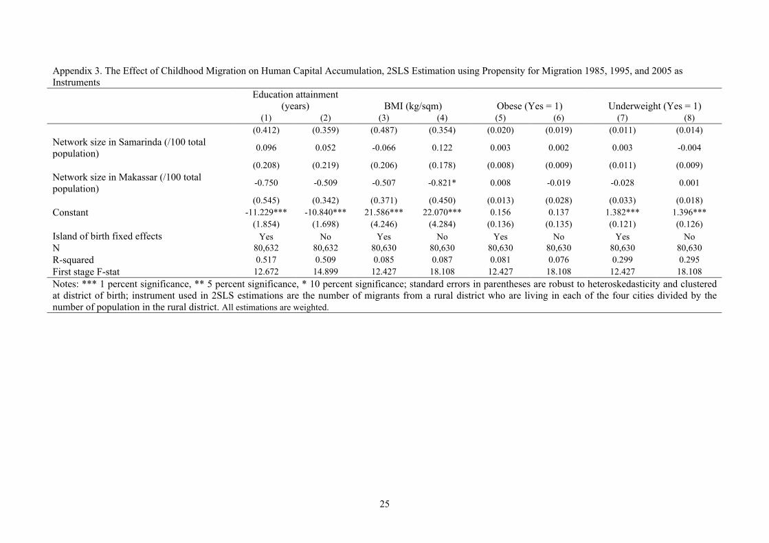
! 25!
Appendix 3. The Effect of Childhood Migration on Human Capital Accumulation, 2SLS Estimation using Propensity for Migration 1985, 1995, and 2005 as Instruments
Education attainment
(years) BMI (kg/sqm) Obese (Yes = 1) Underweight (Yes = 1) (1) (2) (3) (4) (5) (6) (7) (8) (0.412) (0.359) (0.487) (0.354) (0.020) (0.019) (0.011) (0.014) Network size in Samarinda (/100 total population) 0.096 0.052 -0.066 0.122 0.003 0.002 0.003 -0.004
(0.208) (0.219) (0.206) (0.178) (0.008) (0.009) (0.011) (0.009) Network size in Makassar (/100 total population) -0.750 -0.509 -0.507 -0.821* 0.008 -0.019 -0.028 0.001
(0.545) (0.342) (0.371) (0.450) (0.013) (0.028) (0.033) (0.018) Constant -11.229*** -10.840*** 21.586*** 22.070*** 0.156 0.137 1.382*** 1.396*** (1.854) (1.698) (4.246) (4.284) (0.136) (0.135) (0.121) (0.126) Island of birth fixed effects Yes No Yes No Yes No Yes No N 80,632 80,632 80,630 80,630 80,630 80,630 80,630 80,630 R-squared 0.517 0.509 0.085 0.087 0.081 0.076 0.299 0.295 First stage F-stat 12.672 14.899 12.427 18.108 12.427 18.108 12.427 18.108 Notes: *** 1 percent significance, ** 5 percent significance, * 10 percent significance; standard errors in parentheses are robust to heteroskedasticity and clustered at district of birth; instrument used in 2SLS estimations are the number of migrants from a rural district who are living in each of the four cities divided by the number of population in the rural district. All estimations are weighted.


