The Effect of More Accurate Cost-of-Living Indexes on Welfare Recipients

Emily Yucai Wang

March 26, 2018

Abstract

An economic indicator, the Consumer Price Index (CPI), is widely used as a measurement

of inflation. A large literature has accumulated to improve its accuracy, including those focused

on incorporating intertemporal substitution. Most calculations, however, are still based on the

behavior of the average household. This may be problematic since the CPI also plays an impor-

tant role in adjusting payments to millions of social welfare recipients, most of whom differ from

the average in facing more binding budget and space constraints. Both constraints inhibit these

households’ability to stockpile during price reductions. Therefore, switching from a fixed weight

to a more accurate price measurement could significantly underestimate the true cost-of-living

for the welfare recipients. This paper quantifies the welfare impact of this switch by estimating

a dynamic demand model of storable goods. Using a sample of households who qualify for the

Supplemental Nutritional Assistance Program ("Food Stamps"), I find that welfare recipients

may experience a welfare loss of close to 9%.

1

1 Introduction

Over the past ten years, the change in the cost of living for poor households has deviated significantly

away from that of the representative household. The staple portion of households’food basket has

gone up in cost relative to that of an average household. In other words, the trend in the cost of

living for poor households has deviated from that of an average household. This has significant

implications for those households who depend on the social safty net such as the SNAP program,

Disablility Income, and Unemployment Benefits. These programs are adjusted based on the cost

of living for the representative household. As the rate of the cost of living adjustments deviate

between the two groups, poor households, whose livelihood depend more heavily on the cost of

living adjustments are severly impacted.

This paper shows how temporary price reductions (temporary price flactuations) can perversely

negatively impact poor households’welfare. [I feel like I’m missing a couple steps in my argument

here.] Descriptive evidence in the paper shows households whose income falls below the poverty

line, hence forth refered to as poor households, spend more on many storable goods than the average

households. This is driven by the stockpilability of many goods in household’s shopping baskets. [I

could show for many stockpilable goods, poor households end up paying more.]

Taking a structural approach that controls for stockpiliability, I show that holding household’s

utility of the basket of goods constant, it takes more money to sustain the same utility now than a

decade earlier.

2 Background and Data

2.1 Supplemental Nutrition Assistance Program

{What SNAP is} The Supplemental Nutrition Assistance Program administered by the USDA that

provides nutrition assistance to eligible low income households. It is the largest program in the

US federal social safety net for low-income families, serving roughly 46.5 million [double check]

households.

{Who Qualifies for SNAP} To qualify for SNAP, households must satisfy several criteria. The

most important is an income requirement. In general, a household may qualify for benefits if its

gross monthly income is 130% or less the federal poverty level of a specific household size. For

instance, a household with three members earning below $1,591 per month would qualify for SNAP

benefits in 2013. The same household would qualify for the same benefit with a monthly income

of $1,272. In addition to income, households must satisfy requirements on available resources (less

than $2,250 in countable resources for households without one member being at least 60 and $3,250

otherwise). In addition, there are some requirements with regards to employment, disability, and

the elderly.

{How SNAP works} The amount of benefits, an allotment, a household receives is equal to

the maximum allotment amount subtracting a third of the household’s income. For instance, the

2

maximum monthly allotment for a household of three in 2013 is $526. The actual benefit the

household receives is equal to this amount minus 0.3 times the monthly income of the household.

SNAP benefits are distributed on a monthly basis through an electronic benefit transfer (EBT)

system. Through the EBT, a recipient may make purchases at participating retailers to purchase

authorized food items. Per USDA rules, eligible foods include fruits and vegetables, breads and

cereals, dairy products, meats, fish, poultry, and junk food items such as soft drinks, candy, and ice

cream.

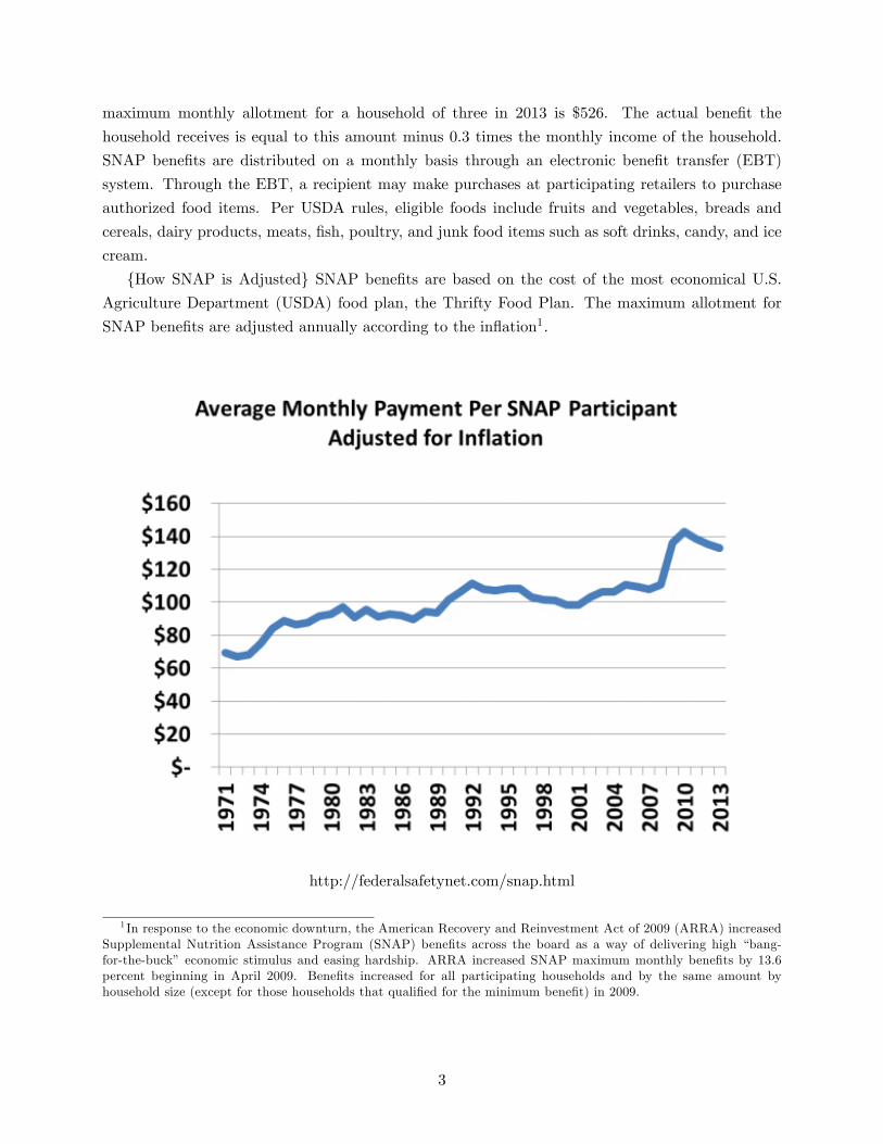
{How SNAP is Adjusted} SNAP benefits are based on the cost of the most economical U.S.

Agriculture Department (USDA) food plan, the Thrifty Food Plan. The maximum allotment for

SNAP benefits are adjusted annually according to the inflation1.

http://federalsafetynet.com/snap.html

1 In response to the economic downturn, the American Recovery and Reinvestment Act of 2009 (ARRA) increasedSupplemental Nutrition Assistance Program (SNAP) benefits across the board as a way of delivering high “bang-for-the-buck” economic stimulus and easing hardship. ARRA increased SNAP maximum monthly benefits by 13.6percent beginning in April 2009. Benefits increased for all participating households and by the same amount byhousehold size (except for those households that qualified for the minimum benefit) in 2009.

3

[old] I use weekly scanner data provided by Information Resources Inc. (IRI) from 2002. The

data is comprised of two components: a household panel and a store panel. The households in the

data set were randomly selected.2 For each household in each week, I observe whether any soda was

purchased; if so, I observe which product was purchased, where it was purchased, how much was

bought, and the total dollar amount paid. From the store panel, in each week, I observe the price

charged, the total quantity sold, and all promotional activities for each product that was sold in

the store. Sales from these stores account for over 97% of all purchases of soft drinks observed from

the households in the panel. There are also two sets of attributes: one set for the households and

one set for the products. For each household, I observe a few basic demographic variables, such as

race, income, and the size of the households. For each product, I observe the product name, brand,

packaging and volume.

For each observation from both the store and the household panel, unique identifiers on the

product, store, and week allows me to link the two sets of data and track prices and promotions

for all products available to households on any given shopping trip. That is, I observe not only

information on the purchase itself but also information regarding each household’s complete choice

set.

Household Panel I group households into two non-mutually-exclusive sets. The first sample

includes only households whose aggregate annual income is below the federal poverty line and has

at least three household members3. Table (1) below provides some information on the 2002 poverty

guidelines along with the number of such households in the sample. The second sample includes all

Table 1: 2002 Household Poverty Guideline

Size of Family Aggregate Income1 Number of HH in Sample3 $15,020 704 $18,100 1145 $21,180 756 $24,260 587 $27,340 N/A2

8 $30,420 N/A2

Total 317

1. Source: U.S. Department of Health and Human Services

2. IRI sample caps family size at 6. Households with more members are encoded as 6.

households in the data. I will refer to sample 1 as the low income households and sample 2 as all

2 IRI randomly selects a sample of households in each of the two suburban areas around the Midwest and NewEngland and requests their participation. The participating households conform to the local demographics fairly well.The data does not suggest a selection bias in the panel.

3 In the data there is a large share of young households with one or two members. These households are unlikelyto be welfare recipients and may still receive help from their parents. Hence, I limit the sample to households with atleast three members.

4

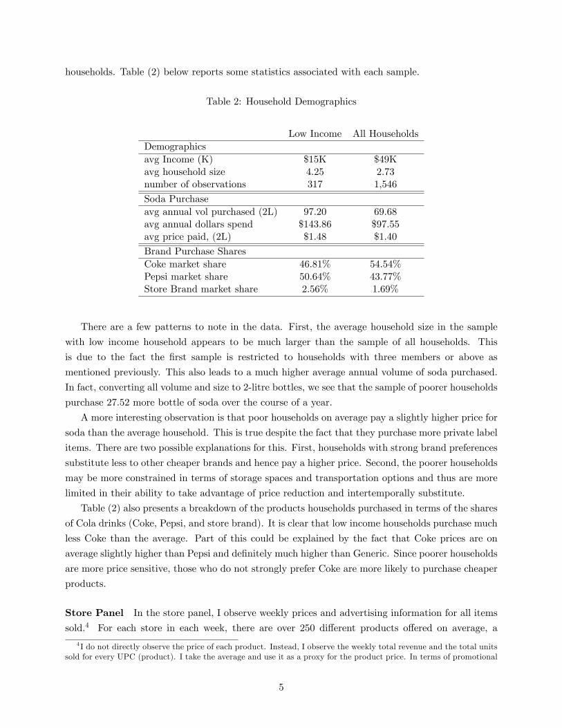
households. Table (2) below reports some statistics associated with each sample.

Table 2: Household Demographics

Low Income All HouseholdsDemographicsavg Income (K) $15K $49Kavg household size 4.25 2.73number of observations 317 1,546

Soda Purchaseavg annual vol purchased (2L) 97.20 69.68avg annual dollars spend $143.86 $97.55avg price paid, (2L) $1.48 $1.40

Brand Purchase SharesCoke market share 46.81% 54.54%Pepsi market share 50.64% 43.77%Store Brand market share 2.56% 1.69%

There are a few patterns to note in the data. First, the average household size in the sample

with low income household appears to be much larger than the sample of all households. This

is due to the fact the first sample is restricted to households with three members or above as

mentioned previously. This also leads to a much higher average annual volume of soda purchased.

In fact, converting all volume and size to 2-litre bottles, we see that the sample of poorer households

purchase 27.52 more bottle of soda over the course of a year.

A more interesting observation is that poor households on average pay a slightly higher price for

soda than the average household. This is true despite the fact that they purchase more private label

items. There are two possible explanations for this. First, households with strong brand preferences

substitute less to other cheaper brands and hence pay a higher price. Second, the poorer households

may be more constrained in terms of storage spaces and transportation options and thus are more

limited in their ability to take advantage of price reduction and intertemporally substitute.

Table (2) also presents a breakdown of the products households purchased in terms of the shares

of Cola drinks (Coke, Pepsi, and store brand). It is clear that low income households purchase much

less Coke than the average. Part of this could be explained by the fact that Coke prices are on

average slightly higher than Pepsi and definitely much higher than Generic. Since poorer households

are more price sensitive, those who do not strongly prefer Coke are more likely to purchase cheaper

products.

Store Panel In the store panel, I observe weekly prices and advertising information for all items

sold.4 For each store in each week, there are over 250 different products offered on average, a

4 I do not directly observe the price of each product. Instead, I observe the weekly total revenue and the total unitssold for every UPC (product). I take the average and use it as a proxy for the product price. In terms of promotional

5

combination of all brands, regular/diet, packaging, volume, and flavors. In the estimation of the

model, prices and promotions of all products become part of the state variables. Carrying prices

and promotions of 250 products is computationally infeasible in the dynamic programming problem.

Hence, I restrict the set of products used in estimation to include all cola products. I allow for

all regular and diet versions of Coca-Cola, Pepsi Cola, and Private Label Cola drinks in different

variations. Cola products are unique in flavor and thus are naturally distinct from other soft drinks.

Alternatives such as lemon-lime soda or root beer are not close substitutes.

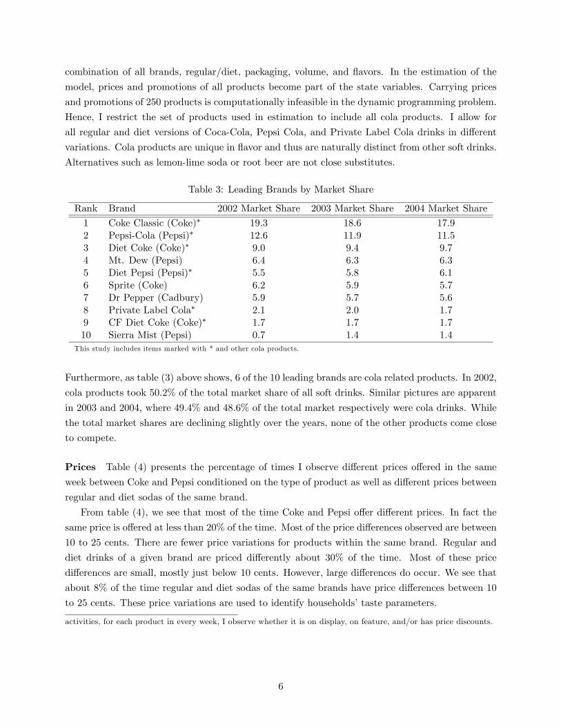
Table 3: Leading Brands by Market Share

Rank Brand 2002 Market Share 2003 Market Share 2004 Market Share

1 Coke Classic (Coke)∗ 19.3 18.6 17.92 Pepsi-Cola (Pepsi)∗ 12.6 11.9 11.53 Diet Coke (Coke)∗ 9.0 9.4 9.74 Mt. Dew (Pepsi) 6.4 6.3 6.35 Diet Pepsi (Pepsi)∗ 5.5 5.8 6.16 Sprite (Coke) 6.2 5.9 5.77 Dr Pepper (Cadbury) 5.9 5.7 5.68 Private Label Cola∗ 2.1 2.0 1.79 CF Diet Coke (Coke)∗ 1.7 1.7 1.710 Sierra Mist (Pepsi) 0.7 1.4 1.4

This study includes items marked with * and other cola products.

Furthermore, as table (3) above shows, 6 of the 10 leading brands are cola related products. In 2002,

cola products took 50.2% of the total market share of all soft drinks. Similar pictures are apparent

in 2003 and 2004, where 49.4% and 48.6% of the total market respectively were cola drinks. While

the total market shares are declining slightly over the years, none of the other products come close

to compete.

Prices Table (4) presents the percentage of times I observe different prices offered in the same

week between Coke and Pepsi conditioned on the type of product as well as different prices between

regular and diet sodas of the same brand.

From table (4), we see that most of the time Coke and Pepsi offer different prices. In fact the

same price is offered at less than 20% of the time. Most of the price differences observed are between

10 to 25 cents. There are fewer price variations for products within the same brand. Regular and

diet drinks of a given brand are priced differently about 30% of the time. Most of these price

differences are small, mostly just below 10 cents. However, large differences do occur. We see that

about 8% of the time regular and diet sodas of the same brands have price differences between 10

to 25 cents. These price variations are used to identify households’taste parameters.

activities, for each product in every week, I observe whether it is on display, on feature, and/or has price discounts.

6

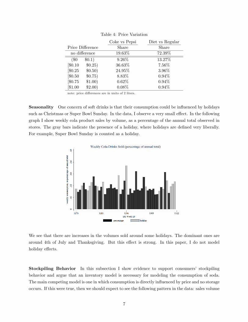
Table 4: Price Variation

Coke vs Pepsi Diet vs RegularPrice Difference Share Shareno difference 19.63% 72.39%

($0 $0.1) 9.26% 13.27%[$0.10 $0.25) 36.63% 7.56%[$0.25 $0.50) 24.95% 3.96%[$0.50 $0.75) 8.83% 0.94%[$0.75 $1.00) 0.62% 0.94%[$1.00 $2.00) 0.08% 0.94%note: price differences are in units of 2 liters.

Seasonality One concern of soft drinks is that their consumption could be influenced by holidays

such as Christmas or Super Bowl Sunday. In the data, I observe a very small effect. In the following

graph I show weekly cola product sales by volume, as a percentage of the annual total observed in

stores. The gray bars indicate the presence of a holiday, where holidays are defined very liberally.

For example, Super Bowl Sunday is counted as a holiday.

We see that there are increases in the volumes sold around some holidays. The dominant ones are

around 4th of July and Thanksgiving. But this effect is strong. In this paper, I do not model

holiday effects.

Stockpiling Behavior In this subsection I show evidence to support consumers’ stockpiling

behavior and argue that an inventory model is necessary for modeling the consumption of soda.

The main competing model is one in which consumption is directly influenced by price and no storage

occurs. If this were true, then we should expect to see the following pattern in the data: sales volume

7

increases when price reductions are available but decreases and remains largely constant when there

is no sale. This, however, is not the case. In the following graph we see that sales volume drops

dramatically immediately after each sale ends; then it slowly grows again. This can be explained

by stockpiling: households fill their inventories during price reductions. Hence, they do not need to

purchase much soda immediately afterwards. As time passes households deplete their inventories.

Therefore, more and more households have to restock.

As an example, I use the sale of regular Coke from a representative store in 2002. This graph shows

how sales volume evolves over the duration of a year and how it is influenced by price reductions.

Each bar shows the sale volume of a week. Black bars indicate price reductions while the gray ones

are used for weeks without sales.

It is clear that the demand for regular Coke dramatically increases when there is a price reduc-

tion. Moreover, we see that the sales volume decreases drastically right after the price reductions;

it picks up again in the following weeks. (These occurrences are marked by the horizontal lines be-

neath the bars.) These dips in purchases are consistent with households stocking up on soda when

there are price reductions, reducing the need for buying soda immediately afterwards. However, as

their stocks run low they make more purchases again. Static models do not account for this effect.

They assume all purchased units are immediately consumed and hence are inherently misspecified.

To further distinguish between static and dynamic behavior I analyze how past prices influence

current purchase size choices. To be more precise, I regress the quantity purchased on prices and the

time since the last sale ("duration"). Table 5 below shows the results from this simple regression:

in a static model, duration should not have any effect; purchase decisions only depend on current

prices and marginal utilities of consumption. However, if the inventory model is correct, purchase

quantities should be greater if more time passed since the last sale. The reason for this is that

households are able to stockpile items not needed for immediate consumption. But when they go

8

Table 5: Regression of Quantity Purchased

Coeffi cient

duration to last sale 10.8128*(3.6670)

price of product 738.137**(14.1617)

constant term −1630.061**(35.1733)

Note: * at 95% significance level and ** at 99% significance level.

through a long time of high prices their inventories are depleted so that it takes a larger purchase

to restock. Indeed, coeffi cients in both regressions are positive and statistically significant. This

shows that purchases are highly correlated with past prices, justifying a dynamic specification.

Persistent Heterogeneous Preferences Lastly, I present evidence for persistent consumer het-

erogeneity. The following table shows the probability of observing brand purchases conditional on

the observed last purchases:

Table 6: Transitional Probability of Purchase

Prob(brand in per. 2 | brand in per.1)Prob(coke|coke) 84.81%Prob(pepsi|coke) 15.19%

Prob(coke|pepsi) 26.66%Prob(pepsi|pepsi) 73.34%

If households do not have intrinsic brand preferences, then the product choice in the second

period should be independent to that of the first. That is the probability of buying product x in

period t+ 1 conditional on buying the same product in period t should be roughly the same as that

conditional on buying product y in period t. However, this is not the case, as seen table (6). The

probability of purchasing Coke in period t+1 conditional on purchasing Coke in period t is 84.81%.

The probability of purchasing Coke in period t + 1 conditional on purchasing Pepsi in period t,

however, is only 26.66%. This suggests that households have persistent brand preferences.

3 Model

In line with Wang (2012), this is a dynamic discrete choice model with random coeffi cients. It flexibly

incorporates observable consumer characteristics as well as unobservable persistent heterogeneity

in preferences. Households in the model are forward looking. They form expectations over future

prices and may choose to build inventories to ward off future price increases. In each period, they

maximize the expected sum of their discounted future utilities by making three decisions: they

9

choose how much they want to consume, how much they want to purchase, and if they chose to buy

anything at all, which product they want to buy. Since soft drinks are storable, households are not

forced to consume everything they purchase. They choose the utility maximizing consumption level

taking prices, promotions, and available inventories into account. All leftover products become part

of the storage for future consumption. Households face two sources of uncertainty in this model:

random and potentially nonlinear future prices (along with promotional activities) and future utility

shocks.

The decision period is one week. In each period, the timing of events goes as follows: first,

households observe their inventory, obtain information on prices and promotional activities of all

products in the market, and receive privately drawn utility shocks associated with consumption

and product choices. With information on the current prices and advertising activities, they form

expectations over future prices and promotions. During their supermarket visits, they choose the

level of consumption and the amount to purchase. Should they make any purchase, households

will base their product choices on their preferences, prices, available promotions, and the previously

drawn shocks. At the end of each period, households incur costs associated with their leftover

inventories.

Broadly speaking, heterogeneity is present in the model in two ways. First, households are

differentiated according to their observable attributes, such as their income, race, etc. Second, they

differ by their unobservable persistent tastes for product characteristics, such as brand, as well as

their sensitivities for prices/advertising and their abilities to stockpile. As shown in the following

subsection, this specification of the unobservable tastes allows for a full correlation structure between

brand preferences. It provides unrestricted substitution patterns across all products and hence

presents a very flexible way of incorporating household taste heterogeneity.

3.1 Model Setup

Household h’s problem can be represented by the following infinite horizon maximization problem:

V h (φ1) = max{ch(φt),s

h(φt),ih(φt)}

∞∑t=1

δt−1E[uhtsi|φ1

](1)

where V h (φ1) denotes household h’s present value of future utility for a given state φt at time

t = 1. The state space for period t, φt, consists of current prices and promotions, the beginning-

of-period inventory, a shock to utility from consumption, and an idiosyncratic shock to utility for

each product. In each period, households maximize their objectives with respect to the level of

consumption ch, the volume of purchase sh, and the product choice ih. I use the standard notation

δ to denote the discount factor and the small letter u for the flow utility, where household h’s flow

utility for period t is defined as:

uhtsi = U(cht , υ

ht |Θh

)− C

(invht+1|Θh

)+ U

(ptsi, atsi, i

htbd, ε

htsi|Θh

). (2)

10

It is comprised of three components: the utility of consumption U(cht , υht |Θh), the cost of inventory

C(invht+1|Θh), and the utility to purchase U(ptsi, atsi, ihtbd, ε

htsi|Θh). The set of household specific

taste parameters is denoted by Θh.

The utility of consumption is a function of cht , the amount household h consumes in period t,

and υht , a stochastic shock to utility that changes the utility from consumption. The consumption

is equal to the total of all i products consumed by household h in period t. That is, cht =∑ichit.

The shock υht households receive in each period introduces randomness in households’ need to

consume and allows their consumption to depend on factors that are unobserved by the researcher.

It influences the utility in the following way. If household h draws a high realization of υht , then its

marginal utility of consumption would be smaller than if a low realization were drawn. Therefore,

a high realization decreases households’need to consume and hence makes demand more elastic. I

make the following assumption regarding υht ’s distribution:

Assumption 1. The consumption shocks, υht , are distributed independently and identically acrosshouseholds and over time.

In principle, serial correlation in υht can be accommodated, but at a significant increase in compu-

tational burden. I follow previous literature in assuming that the utility of consumption takes the

following form:

U(cht , υht |Θh) = αh log(cht + υht ) (3)

where the consumption level and the stochastic shock enter additively into the utility. Unlike

previous literature, I allow the marginal utility of consumption, αh, to be household specific.5

Households’cost of inventory follows a quadratic functional form:

C(invht |Θh

)= βh1 inv

ht + βh2

(invht

)2(4)

where βh1 and βh2 are household specific linear and quadratic cost terms. These parameters represent

households’abilities to store leftover products: households with higher marginal costs of inventory

find storage more costly and hence might not be able to take advantage of sales as readily as

households with lower βh1 and βh2 . Following simple accounting rules, the end-of-period inventory,

invht+1, is equal to the beginning-of-period inventory, invht , plus the total current purchase, s

ht , minus

the total consumption, cht . That is, invht+1 = invht +sht −cht . Since households cannot consume more

than what is available in their storage or make negative purchases, the total inventory, invht , and

purchase, sht , are restricted to be non-negative.

The last piece of the flow utility is associated with household h’s purchase in period t, which

is a function of prices, promotional activities, product preferences, and a random shock to the

5Technically, the marginal utility of consumption is αh/(cht + υht

), which depends on both the consumption level

and the consumption shock. For simplicity, I call αh the marginal utility of consumption.

11

household’s choice. It can be represented as:

U(ptsi, atsi, i

htbd, ε

htbs|Θh

)= −γh1ptsi + γh2atsi +

∑b

1l(bht

)ζhb s

ht + εhtsi, (5)

where −γh1ptsi represents household h’s disutility of price. It is equal to the negative of household h’smarginal utility of income, γh1 , multiplied by the price, ptsi, for product i of volume s in time t. The

second component γh2atsi captures the effect of advertising on demand. Variable atsi is an indicator.

It denotes the presence of any features or displays. Households in the model are forward-looking.

They form expectations over the uncertain future prices and promotions. For simplicity, I assume

the transitions of these prices and promotions follow the assumption below:

Assumption 2. Prices and advertising activities follow an exogenous first order Markov process.

This assumption is often employed in the empirical literature to reduce the state space in the

dynamic programming problem. It is a simplifying assumption on households’ expectations for

future prices and promotions and implies that consumers use only the current period prices and

promotions in predicting future prices and promotion. This assumption seems to be a reasonable

approximation of the formation of consumers’ price expectations. Higher order processes would

require households to recall more prices from previous visits. The main concern might be seasonal

price fluctuations, when the probability of advertising increases. However, as described in the data

section, there is no clear evidence of significant seasonal effects in the household panel. The third

component, 1l(bht)ζhb s

ht , represents household h’s utility for consuming s units of brand b in time t. It

is equal to household h’s intrinsic preferences for brand b, ζhb , multiplied by the volume purchased,

sht , in period t. The last component, εhtsi, denotes an idiosyncratic shock to household h’s product

choice, which follows the commonly used distribution in discrete choice problems:

Assumption 3. The product choice shocks, εhtsi, follow a type I extreme value distribution and areindependent and identically distributed across household, period, and purchase.

The idiosyncratic shock absorbs the apparent randomness in consumers’purchases that are based on

factors unobserved by the econometrician. This assumption significantly reduces the computational

burden. It could be relaxed; however, since households’product preferences are explicitly estimated

and the volumes of purchases are allowed to be correlated across periods, assuming the shock is

i.i.d. across households, time, and purchase is reasonable.

In line with Hendel and Nevo (2006b) and Wang (2012), product differentiation in this model

takes place at the moment of purchase. While households have intrinsic preferences for different

brands and diet drinks, these preferences and the differences between products affect households’

behaviors exclusively at the store but do not give different utilities at the moment of consump-

tion. Since consumptions and inventories are not observed, this specification avoids putting extra

structure on consumption rates of different items in the inventory. Furthermore, this assumption

significantly decreases the state space. Instead of carrying the whole vector of inventories for each

12

brand, only the total quantity in stock is tracked. Differentiation at purchase, represented by

1l(bht)ζhb s

ht captures the expected value of the future differences in utility from consumption. More

specifically, the term ζhb sht captures the expected utility from future consumption of s units of brand

b at the time of purchase.

4 Estimation

Solving the infinite horizon maximization problem faced by each household in each period can

be computationally demanding and time consuming, especially in the presence of a large state

space. Several key factors of the model further complicate this process. First, current period

inventories are unknown since neither consumption levels nor initial inventories are observed. To

calculate the current inventory, both the current consumption and the initial inventory have to be

estimated. Second, since all parameters are random coeffi cients, the likelihood has to be integrated

over the joint distribution of these parameters. The necessity of having to solve the consumers’

dynamic programming problem at every guess of the parameters and for each possible consumption,

inventory level, and product choice presents a significant computation burden. Using traditional

maximum likelihood methods implies that the estimation for a set of parameters would take months

to compute. I nest a simulated maximum likelihood approach into the importance sampling method

introduced by Ackerberg (2009) to reduce the computation time. I start the discussion of the

estimation by providing an overview and then move on to a more detailed description of the technical

details.

4.1 Overview

Recall from the data section that we observe only the purchases by households over time. In

each period, we know whether household h made any purchases. If a purchase was made, then we

observe which product was purchased and how many units were bought. However, no information is

available on households’consumptions, inventories, or their intrinsic tastes. The goal is to maximize

the probability of observing this sequence of purchases with respect to the parameters that govern

the distribution of the random coeffi cients, the initial inventory, as well as the distribution of

household type.

Assume for now that we are in a world where the econometrician observes not only the pur-

chases but also both the households’preferences and their initial inventories. Then, for a given set

of parameters, the probability of observing a sequence of purchase decisions, purht , across all house-

holds and over time,(pur1

1, · · · , pur1T , . . . . . . , pur

H1 , · · · , purHT

), as a function of the state variables,(

φ1t , · · · , φHt

), is given by the following integral:

L =

∫Θh

Pr(pur1

1 · · · purHT |φht , invh0 ,Θh)dF(

Θh|µΘ,ΣΘ

)where φht =

{pt,at, υht , inv

ht

(purh1 · · · purht−1, υ

h1 · · · υht−1, inv

h0

)}13

The state φht includes the vector of prices and promotions, pt and at; the current period consumption

shock, υht ; and the beginning of the period inventory, invht . The inventory is a function of previous

decisions and states. It depends on last period’s consumption and purchase decisions, which in turn

depends on the consumption shocks and the idiosyncratic purchase shocks of that period as well as

all earlier periods’inventories.

Assuming households are independent from each other, the probability of observing a sequence

of purchases from household h is then independent from that of household h′. Hence, the probability

of observing the entire purchase sequence of all households can be re-written as:

L =H∏h=1

∫Θh

Pr(purh1 , · · · , purhT |φht , invh0 ,Θh

)dF(

Θh|µΘ,ΣΘ

)(6)

Furthermore, recall that purchases can be decomposed into product purchases, iht , and volume pur-

chases, sht . That is Pr(purh1 , · · · , purhT |φht , invh0 ,Θh

)= Pr

(sh1 · · · shT , ih1 · · · ihT |φht , invh0 ,Θh

). Since

the product choice shocks are i.i.d., households’brand purchases are independent over time. There-

fore rewriting the probability of observing the sequence of purchases once again, we arrive at:

L =

H∏h=1

∫Θh

[T∏t=1

Pr(iht |sht , φht ,Θh

)]Pr(sh1 · · · shT |φht , invh0 ,Θh

)dF(

Θh|µΘ,ΣΘ

)(7)

From this equation, it is straight forward to see that household’s two purchase decisions, product

and size, are treated differently. The product choices, iht , are uncorrelated across periods, hence the

decision making process is static. That is, conditional on households’ intrinsic preferences, their

product choices in period t are independent from those in period t+ 1. By assumption 3, product

shocks are distributed according to a Type I extreme value distribution. Therefore, the probability

of seeing any particular purchase follows the standard logit formula:

Pr(iht |sht , φht , τh,Θh

)=

exp[(−γh1ptsbd + γh2atsbd +

∑b 1l(bht)ζhb s

ht

)]∑b

∑d exp

[(−γh1ptsbd + γh2atsbd +

∑b 1l(bht)ζhb s

ht

)] (8)

The volume purchase decisions, sht , on the other hand, depend on current consumption as well

as past consumption levels, purchase decisions, and initial inventories. Consumptions and volume

purchases are determined by households’optimal policies and are correlated over time. Hence, the

probability of observing any sequence of volumes purchased depends on that household’s optimal

policy rule, which is a dynamic programming problem and cannot be estimated separately for each

period.

Recall, households’consumption shocks, υht , and initial inventories, invh0 , are not actually ob-

served. Therefore, to estimate the model, we need to integrate equation (7) over the distribution of

14

consumption shocks and initial inventories. Mathematically, this can be expressed as:

L =H∏h=1

∫

Θh

∫υ

∫inv0

(T∏t=1

Pr(iht |sht , φht , invh0 ,Θh

)Pr(sh1 · · · shT |φht , invh0 ,Θh

))(9)

dF(invh0

)dF(υh1 · · · υhT

)]dF(

Θh|µΘ,ΣΘ

)}

Calculating the above likelihood function is a 2-step process. First, solve the dynamic programing

problem and find the optimal policy rule that govern households’optimal consumption and purchase

choices. Second, compute households’choice probabilities. Both of steps are carried out for each

household, consumption shock, initial inventory, and parameter try. This becomes a very time

consuming process. Part of the computation burden comes from the unobserved initial inventory;

part from the random coeffi cients whose parameters govern the distribution of households’persistent

preferences; and part from carrying a large state space. I discuss these complicating factors in detail

below.

Households’ initial inventories are unknown to the econometrician and hence need to be esti-

mated. Assume, for now, that we observe households’ inventory at the beginning of period one.

Then once the optimal consumption and purchase choices are estimated, we can calculate the end

of period inventories for the first period. Roll this process forward and we can obtain all inventories

across all periods. Estimating the entire sequence of inventories boils down to an initial conditions

problem.

One way of estimating the initial inventory is to start at an arbitrary level and use the first few

weeks of observations to generate the distribution of inventories. To obtain a good estimate using

this method, the panel has to be relatively long. For example, Hendel and Nevo (2006b) take this

approach. Their panel spans 2 years and they use the first 11 weeks to recover estimates for the

initial inventories. In this paper, however, the length of panel is one year. Hence, I adopt a different

approach. I use the model and observed households’purchase behaviors to explicitly estimate a

distribution over the initial inventory. I assume initial inventories follow the distribution specified

below:

Assumption 4. The initial inventories invh0 are distributed log-normal with mean µinv and standarddeviation σinv.

Households’ persistent preferences are also unobserved. These heterogeneous preferences are

modeled using random coeffi cients which follow distributions whose parameters are estimated in

the model. I assume the distribution follows the assumption below:

Assumption 5. The random coeffi cients Θh ={αh, βh1 , β

h2 , γ

h1 , γ

h2 , ζ

hC , ζ

hP

}are distributed jointly

log-normal with mean µΘ and variance-covariance matrix ΣΘ.

These random parameters capture households’persistent heterogeneous tastes. Since the econo-

metrician does not observe them, the joint distribution of these preferences is estimated. These

15

parameters are naturally bounded on either side of the real line. For example, the marginal utilities

of consumption are non-negative. Hence, the log normal distributions are fitting. I further assume

that the off diagonal elements of the variance-covariance matrix are zero. This restriction can be

lifted at the cost of an increased computation burden.

Solving the dynamic programming problem and calculating the choice probabilities for one

household at an initial inventory level for a given set of parameter try is not time consuming, per

se. This process takes roughly 10 seconds once.6 However, if we adopted the standard maximum

likelihood estimation approach, this computation process is repeated for each household, initial

inventory guess, and parameter try.7 The repetition quickly increases the computation time to

become unmanageable. I adopt a simulated maximum likelihood approach and build on the impor-

tance sampling method proposed by Ackerberg (2009) to significantly cut down computation time.

In estimating this model, allowing for parallel computing on 8 cores, the entire estimation process

takes about 3 days.

The reduction in computation time predominantly comes from the fact that importance sampling

allows computing the value functions and the choice probabilities to be performed outside the

maximization routine. This speeds up the calculation in two ways: 1) it allows for easy parallel

computing of all dynamic programming problems across all different household types and parameter

draws; this further allows the set of choice probabilities for all households and all parameter tries

to be computed simultaneously. 2) since the value function calculations are not nested within each

parameter search, the search routine costs very little time. I fully describe the estimation procedure

below.

4.2 Estimation Procedure

The estimation procedure can be roughly broken into five steps.

Step 1 (Initial Parameter Distribution) Importance sampling methods require specificationsof initial distributions over parameters, which are updated during the convergence process. The

initial distributions can be chosen arbitrarily at the discretion of the econometrician as long as

they have a fairly large range that well covers the true parameter value.8 To start the estimation

process, I pre-define an initial joint distribution of the random coeffi cients, g(

Θh∣∣µ0

Θ,Σ0Θ

), and a

distribution over the initial inventory, g(inv0

∣∣µ0inv0

, σ0inv0

), where the parameters that govern these

distributions,(µ0

Θ,Σ0Θ

)and

(µ0inv0

, σ0inv0

), are chosen arbitrarily. Then I draw N sets of parameter

values and initial inventories according to the pre-defined distributions. I denote the randomly

drawn parameters by Θh and the randomly drawn initial inventory by inv0.

6Using a standard PC with 8 cores and 2.80GHz.7Recall that there are roughly 800 households in the data and 9 possible household types. Even at a convergence

criterion of 1e-3, the maximization routine generally takes at least 3000 iterations. That is, the calculation is repeatedat least 21 million times and thus takes 216 million seconds, which is about 6 years.

8 It’s important to choose distributions that have a suffi ciently large variance. Otherwise, certain parameters maybe excluded from being drawn. This would lead to misestimation if the true parameters lay outside the range of theinitial parameter draws. For a discussion of how to choose initial distributions, refer to Ackerberg (2009).

16

Step 2 (Product Choice) With the randomly drawn parameter tries, we can calculate the dy-namic programming problem and compute the choice probabilities associated with each household’s

observed sequence of purchases. Recall, household’s purchase decisions are decomposed into a prod-

uct choice, a static component, and a volume choice, a serially correlated component. Since product

choices are static, conditional on the quantity purchased, they follow the standard logit formula.

For each household, household type, and parameter draw, the probability of observing any product

choice is:

Pr(iht |φ, sht , Θh

sim

)=

exp[(−γhptsbd + γhatsbd +

∑b 1l(bht)ζh

b sht

)]∑

b

∑d exp

[(−γhptsbd + γhatsbd +

∑b 1l(bht)ζh

b sht

)]Step 3 (Dynamic Programming Problem) Households’decisions on how much to purchase

depend on their current level of inventory, which in turn depends on past consumption and purchase

decisions. Hence these volume choices are correlated over time. The Bellman equation equivalent

to households’infinite horizon maximization problem is:

V(φh1

)= max

{c,s,i}

{[αh log

(c+ υh

)−(βh

1 inv′+ β

h

2 inv′2)− γh1psi + γh2asi +

∑b

1l(bh)ζh

b sh + εhsi

]

+δE

[V

((φh)′)|φh1 , c, s, i

]}. (10)

The statespace associated with this model is large. It encompasses not only all prices and promo-

tional activities of all products and sizes but also the consumption shocks and initial inventories. To

be able to estimate the I approximate the expected future utilities by using the sieve value function

iteration method developed in Arcidiacono, Bayer, Bugni, and James (2012).9 To most accurately

approximate the dynamic programming problem, I use all interactions.

With the computed optimal consumption and purchase decisions, the probability of observing

9 In comparing the approximation with the exact solution obtained from policy function iteration using a simplermodel on a smaller state space, I find the EV obtained by sieve value function iteration closely approximates theexactly calculated solution.

17

any sequence of volume purchases, for a given household type and parameter draw, is:

Pr(sh1 · · · shT |φht , invh0 ,Θh

)=

∏t

Pr(sht |pt, υht , invht

(sh1 · · · sht−1, υ

h1 · · · υht−1, inv

h0

),Θh

)where Pr

(sht |pt, υht , invht

(sh1 · · · sht−1, υ

h1 · · · υht−1, inv

h0

),Θh

)(11)

=

maxcht

{uht + δE

[V((φh)′) |φh, cht , sht ]}

∑s

{maxcht

{uht + δE

[V((φh)′) |φh, cht , sht ]}

}

After combining both components of households’purchase decisions, calculating households’choice

probabilities is fairly straight forward.

Step 4 (Choice Probability) For each subset of household and parameter draws, the choiceprobabilities conditional on household h’s type and its beginning-of-period inventory is given by:

Lhsim

(purh1 · · · purhT |φht , invh0 , τh,Θh

)=

[∏t

Pr(iht |φh, sht , Θh

sim

)]Pr(sh1 · · · shT |φht , invh0 , Θh

sim

)(12)

This conditional choice probability is equal to the probability of observing a sequence of product

choices conditional on a sequence of observed volume purchases multiplied by the probability of

observing that particular sequence of volume purchase. To remove some of the conditioning ar-

guments, integrate the above over initial inventories and consumption shocks for each parameter

draw:

Lhsim

(purh1 · · · purhT |φht , Θh

sim

)=

∫υ

∫inv0

Lhsim

(purh1 · · · purhT |φht , invh0 ,Θh

)dF(invh0

)dF(υh1 · · · υhT

)(13)

Therefore, each household has a set of choice probabilities, one for each parameter draw.10 The

objective of the calculations is to find the parameters that maximize the total likelihood.

Step 5 (Log Likelihood Function) To compute the total likelihood function, randomly select asubset of the parameter draws along with their corresponding choice probabilities for each household.

The simulated maximum likelihood function is a weighted average of all the randomly selected choice

10Recall, N is the number of parameter draws specified by the econometrician. In the estimation, I use N = 10, 000.

18

probabilities across all households. That is,

L =H∏h=1

1

#draws

∑#draws

Lhsim (purh1 · · · purhT |φht , Θhsim

) h(Θhsim |µΘ,ΣΘ

)g(

Θhsim

∣∣µ0Θ,Σ

0Θ

) (14)

where h(

Θhsim |µΘ,ΣΘ

)denotes the estimated distribution over random coeffi cients and over initial

inventories. The component h(

Θhsim |µΘ,ΣΘ

)/g(

Θhsim

∣∣µ0Θ,Σ

0Θ

)can be seen as a weight on the

likelihood. Parameters are allocated more weight if they explain households’decisions well. Note,

since all the choice probabilities are calculated prior to maximization, Lhsim(purh1 · · · purhT |φht , Θh

sim

)is nothing more than a large matrix of values. Moreover, since g

(Θhsim

∣∣µ0Θ,Σ

0Θ

)is pre-defined, the

maximization routine updates only the weight h(

Θhsim |µΘ,ΣΘ

).

4.3 Parameter Estimates

As described in the introduction, the estimation routine is performed on two samples. The first is a

sample of 317 households. These are households whose annual incomes are below the federal poverty

line. The second sample includes all 1,546 households who have met the IRI reporting criterion.

However, due to the size of the state space and its associated computation burden, I include only

households who have made purchases of no more than 8.5 litres11 per shopping trip. Packaging of

all types, i.e. bottles or cans, are included in the sample. This limitation excludes around 3% of all

households from the original sample but does not limit households’inventory buildup. Households

may go shopping on two consecutive days or may choose to consume little. Over time, this leads to

substantial inventories.

Table (7) presents the mean and the standard deviation that govern the distribution of all

parameters. for each parameter. Recall that all parameters in the model are random coeffi cients.

Estimates for different income brackets are listed in separate columns.

The parameter estimates roughly conform to our intuition. For instance, comparing poor house-

holds to the entire sample, the average poor household has a slightly higher marginal utility of income

and hence value money more than the average household in the sample. This result is consistent

with decreasing marginal utility of income: as households’income per capita increases, money be-

comes less important for them. The same pattern holds for the utility of promotions: low income

households have a larger affi nity for promotional activities than the average. Poor households also

have a slightly higher marginal utility of consumption. This implies that holding the cost of inven-

tory constant, these households would consume more soda than the average household. The cost of

inventory has an opposite story. Poor households have a higher cost of inventory. It seems that it

is more diffi cult for poor households to stock up than for the average household.

In terms of persistent brand preferences, there is little difference between Coke and Pepsi for

low income households. While the data suggests that these households tend to purchase Coke a bit

11This is roughly equavalent to either 4 units of the standard 2-litre bottles or a pack of 24 cans.

19

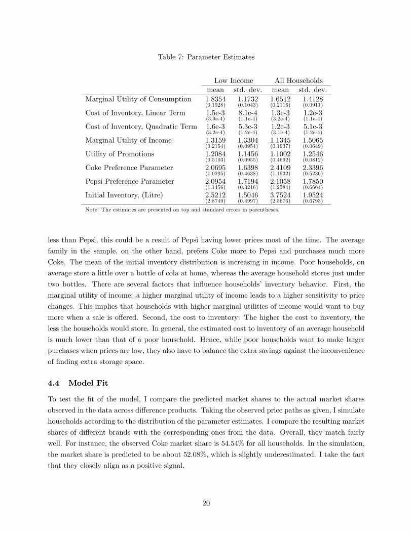
Table 7: Parameter Estimates

Low Income All Householdsmean std. dev. mean std. dev.

Marginal Utility of Consumption 1.8354(0.1928)

1.1732(0.1043)

1.6512(0.2116)

1.4128(0.0911)

Cost of Inventory, Linear Term 1.5e-3(3.9e-4)

8.1e-4(1.1e-4)

1.3e-3(3.2e-4)

1.2e-3(1.1e-4)

Cost of Inventory, Quadratic Term 1.6e-3(3.2e-4)

5.3e-3(1.2e-4)

1.2e-3(3.1e-4)

5.1e-3(1.2e-4)

Marginal Utility of Income 1.3159(0.2154)

1.3304(0.0954)

1.1345(0.1937)

1.5065(0.0649)

Utility of Promotions 1.2084(0.5103)

1.1456(0.0955)

1.1002(0.4692)

1.2546(0.0812)

Coke Preference Parameter 2.0695(1.0295)

1.6398(0.4638)

2.4109(1.1932)

2.3396(0.5236)

Pepsi Preference Parameter 2.0954(1.1456)

1.7194(0.3216)

2.1058(1.2584)

1.7850(0.6664)

Initial Inventory, (Litre) 2.5212(2.8749)

1.5046(0.4997)

3.7524(2.5676)

1.9524(0.6793)

Note: The estimates are presented on top and standard errors in parentheses.

less than Pepsi, this could be a result of Pepsi having lower prices most of the time. The average

family in the sample, on the other hand, prefers Coke more to Pepsi and purchases much more

Coke. The mean of the initial inventory distribution is increasing in income. Poor households, on

average store a little over a bottle of cola at home, whereas the average household stores just under

two bottles. There are several factors that influence households’ inventory behavior. First, the

marginal utility of income: a higher marginal utility of income leads to a higher sensitivity to price

changes. This implies that households with higher marginal utilities of income would want to buy

more when a sale is offered. Second, the cost to inventory: The higher the cost to inventory, the

less the households would store. In general, the estimated cost to inventory of an average household

is much lower than that of a poor household. Hence, while poor households want to make larger

purchases when prices are low, they also have to balance the extra savings against the inconvenience

of finding extra storage space.

4.4 Model Fit

To test the fit of the model, I compare the predicted market shares to the actual market shares

observed in the data across difference products. Taking the observed price paths as given, I simulate

households according to the distribution of the parameter estimates. I compare the resulting market

shares of different brands with the corresponding ones from the data. Overall, they match fairly

well. For instance, the observed Coke market share is 54.54% for all households. In the simulation,

the market share is predicted to be about 52.08%, which is slightly underestimated. I take the fact

that they closely align as a positive signal.

20

Table 8: Observed and Predicted Market Shares

Low Income All HouseholdsObserved Predicted Observed Predicted

Coca Cola 46.81% 48.01% 54.54% 52.08%Pepsi Cola 50.63% 50.77% 43.77% 46.65%Store Brand 2.52% 1.22% 1.77% 1.27%

4.5 Identification, Heterogeneity, and Standard Errors

4.5.1 Identification

I now briefly and informally discuss the identification of the model. The identification of the

static parameters follows the standard arguments (See Bajari, Fox, Kim, and Ryan (2012) for a

detailed discussion on the identification in random coeffi cient logit models). Parameters governing

households’sensitivities to prices and advertising are identified from variations over time in prices

and promotional activities. As price reductions are not perfectly correlated with products on feature

or on display, the effects can be separately identified. The unobservable persistent household taste

parameters are identified off households’purchase behaviors as prices and promotions change over

time. Consider the case where we observe a household consistently purchasing Coke even during

most sales of Peps. For households such as this, we can conclude that it has a strong preference for

Coke.

Similar to Hendel and Nevo (2006b) the identification of the dynamic parameters is more subtle.

The complication arises from the fact that neither the consumption nor the inventory is observed.

If both were observed, then the identification would follow standard arguments. (See Aguirregabiria

(2005), Magnac and Thesmar (2002), and Rust (1996)). To recover the utility of consumption and

the cost of inventory, I rely on the relationship between current purchases, previous purchases, and

prices. Given the process of prices and advertising, preferences, storage costs, and initial invento-

ries determine consumer purchases. For a given storage cost function, the utility of consumption

determines the level of demand. That is, households with a high utility of consumption will pur-

chase more on average. Hence, if we observe a household making large purchases frequently, we

may conclude that the household has a high utility of consumption. For a given preference, storage

costs determine interpurchase duration and the extent to which consumers can take advantage of

price reductions. Here consider the case of no storage, or very high storage cost. Such households

cannot exploit the price reduction opportunities and stock up on their preferred products. Their

interpurchase durations are dependent only on current prices but not past prices. Hendel and Nevo

(2006b) provide a more in depth discussion of the identification of dynamic parameters.

4.5.2 Heterogeneity

Heterogeneity in product preferences or marginal impacts of prices and promotions can lead to

interesting dynamics. For instance, consider a household with a high unobservable preference for

21

Coke. This household is likely not to react to sales on other products and instead chooses to wait

for regular Coke to go on sale. Suppose the inventory of this household runs low, it may purchase

small amounts of an alternative while waiting for the price of Coke to decrease. Previous models

are unable to accommodate this feature due to the computation intensive nature of the problem.

Accounting for unobservable persistent preferences such as the example above is computation-

ally demanding. Indeed, as pointed out by Hendel and Nevo (2006b), in allowing random effects in

product preferences or marginal impacts of prices, the taste parameters are solutions to dynamic

programming problems instead of being static parameters. That is, to compute the choice proba-

bilities associated with the model unconditional on the unobservable preferences implies integrating

over the distribution of the preferences. The probability of product choice conditional on size pur-

chased and conditional on the preferences of consumers will still be independent of the various

dynamic components. However, to compute the probability of the product choice conditional on

size (but unconditional on persistent preferences) we would have to integrate over the distribution

of preferences conditional on the size purchased. Solving for this distribution requires solving the

dynamic programming program. In this paper, I estimate a model similar to that in Wang (2012),

which allows for a flexible form of the unobservable persistent preferences.

4.5.3 Standard Errors

Standard errors were calculated by random subsampling without replacement. I follow Politis and

Romano (1994) and randomly drew subsamples of 100 households 500 times.

5 Policy Study

Currently, the CPI is calculated using weighted average monthly prices and hence does not capture

intertemporal substitution. In the presence of storable products with frequent and periodic price

reductions this measurement is biased upward. To be more specific, households may purchase

goods when they are on sale and store them for later use. Failing to account for this behavior the

CPI would consistently overestimate the prices paid for such products. Along with the increasing

availability of household and store scanner data, as well as the development of techniques that allow

estimation of sophisticated dynamic models of consumer behavior, more and more research is being

conducted to better track and approximate the price movements of household purchases. These

methods are able to accommodate intertemporal substitution and capture the actual prices paid.

If these changes in the methodology were adopted by social programs to approximate the cost-of-

living, they could have profound implications on the wellbeing of households who depend on social

welfare programs such as the Supplemental Nutritional Assistance Program (SNAP). Assuming

poor households have similar purchase behaviors as any representative household, more accurate

measurements of food costs will likely imply a decrease in welfare payment. In this section, I quantify

the effects of a more accurate measurement of the cost-of-living-index on poor households’welfare.

I calculate poor households’welfare in two situations: one with the actual observed prices and one

22

with monthly average prices. The monthly averages reflect the current CPI method of determining

price levels. The difference between the utilities achieved under the actual observed prices and the

monthly average prices is the welfare loss poor households would experience should social welfare

programs adopt a cost-of-living measurement that takes intertemporal substitution into account.

Using the estimated parameters from the sample of households who earn below the federal

poverty line, I first simulate the purchase and consumption behaviors of a set of 1,000 households

using sequences of observed prices from the 2002 store panel. I further calculate and record the total

utility each household achieves in the year. This provides a distribution of utilities households would

experience under real prices. Then using the same 1,000 households, I alter the price sequences and

instead use a monthly average price for each product. To be more specific, following the practice

used in sampling prices for the CPI, for each product I take the average of all prices observed

across all the stores in a market in the first week of a month and use this average price in simulating

households’consumption and purchase behavior for the month. As previously, I calculate and record

the total utility each household achieves. I compare the average of these two distributions of utility.

I find that on average, poor households achieve a 6% higher welfare under constant price estimates.

That is to say, if social welfare programs switch from an average price based measurement such as

CPI to a more accurate estimate of cost-of-living, using a sample of only households who qualify

for social welfare programs, then households on welfare would experience a 6% welfare loss on

average. This result comes from the fact that poor households reduce their cost-of-living through

intertemporal substitution, which the current method of calculating the CPI does not take into

account. Unfortunately, this result can be misleading, since price indices are usually estimated not

using only poor households but all representative households.

The CPI does not only serve as inflation adjustment for social welfare, it is also used for many

other purposes. And as such the weights used in calculating the CPI are estimated using a sample

of randomly selected households. Comparing these households to households who need federal

assistance, the average household tends to be less price elastic but also has a smaller cost to storage.

They tend to live in larger homes and have better transportation options. These factors allow the

average household to take advantage of sales more and hence on average pay less than the poorer

households who lack these provisions. Indeed, from Table(9) below we see that the average price

an average family pays is above that paid by poorer households.

Table 9: Average Prices Paid

Low Income All Households

Average Price Paid, (2L) $1.48($0.53)

$1.40($0.31)

Note: Difference significant at 95% level.

This is all the more surprising since the average family tends to have a higher persistent brand

preference for Coke, which is usually more expensive. It can be explained by poorer households’

limited ability to stock up and hence end up paying higher prices. From the estimated parameters,

23

we see the initial inventory distribution has a higher mean for the sample with all households than

for the sample with only poorer households. Given that poor households seem to benefit less than

the average from stockpiling, this means that poor households’welfare could be reduced further

should an accurate measure of the cost-of-living be employed on a representative sample of all

households.

To estimate this effect, I repeat the above exercise. Using estimated parameters, this time from

the estimation on the entire sample, I again simulate the consumption and purchase behaviors of

1,000 households under two different sequences of prices. The first is a set of randomly drawn

price sequences from observed store data and the second a monthly average across stores for each

product. I find that the average utility of a representative household, under actual pricing, is over

15% that of monthly average prices. This would suggest that should we use cost-of-living measures

that account for intertemporal substitution on a sample of all households welfare recipients could

be substantially negatively impacted.

6 Concluding Remarks

Previous literature has shown that the current way of calculating the CPI is flawed by not taking

households’substitutions into account. With the ubiquity of scanner data and powerful computers

this could be remedied easily. I develop and estimate a dynamic demand model for storable goods

to study how the welfare recipients would be affected if a more accurate index accounting for

households’ability to stockpile were introduced.

I find that such a change would hurt poor households in two ways: First, the current fixed weight

CPI does not take inventories and households’ability to intertemporally substitute into account;

this means that it assigns too little weight to low prices and thus overestimates the cost of living.

Therefore, introducing a more accurate cost-of-living measurement would result in reduced welfare

payments.

Second, since the CPI is calculated using a sample representative for the whole population,

welfare recipients would suffer an even greater loss. The average household can exploit intertemporal

prices fluctuations more heavily than poor households due to larger homes, better transportation

options, and the lack of binding budget constraints. Thus, calculating the CPI off a sample of all

households could severely underestimate prices paid by poor households and thus lead to even larger

payment reductions.

Together, these findings show that we have to tread carefully when adjusting inflation measures.

As long as the CPI has multiple uses there is a trade-off between accuracy and preserving social

benefits. The most logical conclusion seems to be to introduce a separate cost-of-living measure for

welfare recipients.

24

References

[1] Ackerberg, D. A.(2009). A new use of importance sampling to reduce computational burden in

simulation estimation. QME: Quantitative Marketing and Economics, 7(4), pp 343-376.

[2] Boskin, M., E. Dulberger, R. Gordon, Z Griliches, and D. Jorgenson (1998) “AssociationCon-

sumer Prices, the Consumer Price Index, and the Cost of Living", The Journal of Economic

Perspectives, Winter, Vol. 12, No. 1, pp. 3-26.

[3] Bajari, P., J. Fox, K. Kim, and S. Ryan (2012) “The Random Coeffi cients Logit Model is

Identified", Journal of Econometrics, February, Volume 166 (2), pp. 204-212.

[4] Bajari, P. and L., Benkard (2005): “Demand Estimation with Heterogeneous Consumers and

Unobserved Product Characteristics: A Hedonic Approach,” Journal of Political Economy,

Vol. 113, No. 6.

[5] Benitez-Silva, H., G. Hall, G. Hittsch, G. Pauletto, an J. Rust (2000): “A Comparison of

Discrete and Parametric Approximation Methods for Continuous-State Dynamic Programming

Problems”mimeo, Yale University.

[6] Berry, S., J. Levinsohn, and A. Pakes (1995): “Automobile Prices in Market Equilibrium,”

Econometrica, 63, 841-890.

[7] Bresnahan, T.F. (1981): “Departures from Marginal Cost Pricing in the American Automobile

Industry: Estimates for 1997-1978,”Journal of Industrial Economics, 17, 201—277.

[8] Conlon, C (2010): “A Dynamic Model of Costs and Margins in the LCD TV Industry,”mimeo.

[9] Erdem, T., S. Imai, and M. Keane (2003): “Consumer Price and Promotion Expectations: Cap-

turing Consumer Brand and Quality Choice Dynamics under Price Uncertainty,”Quantitative

Marketing and Economics, 1, 5-64.

[10] Feenstra, R. and M. Shapiro (2003): “High-Frequency Substitution and the Measurement of

Price Indexes,”Univ. of Chicago and NBER. in Robert Feenstra and Matthew Shapiro (eds.),

Scanner Data and Price Indexes.

[11] Goettler, R. and B. Gordon (2011): “Does AMD Spur Intel to Innovate More?,” Journal of

Political Economy, Vol. 119, No. 6, pp. 1141-1200.

[12] Gowrisankaran, G. and Rysman (2011): “Dynamics of Consumer Demand for New Durable

Goods,”mimeo.

[13] Hartmann, W (2006): “Intertemporal effects of consumption and their implications for demand

elasticity estimates,”Quantitative Marketing and Economics, Vol 4, No. 4, 325-349.

[14] Hausman, J (1998): “New Products and Price Indices,”NBER, Retrieved on Nov 14, 2012,

from http://www.nber.org/reporter/fall98/hausman_fall98.html.

25

[15] Hartmann, W. and H. Nair (2010) : “Retail Competition and the Dynamics of Consumer

Demand for Tied Goods,”Marketing Science, Volume 29 Issue 2, March 2010.

[16] Hendel, I. and A. Nevo (2006a): “Sales and Consumer Inventory,”Rand Journal of Economics,

Vol. 37, No.3, Autumn 2006 pp.543-561.

[17] Hendel, I. and A. Nevo (2006b): “Measuring the Implications of Sales and Consumer Inventory

Behavior,”Econometrica, Vol. 74, No.6, 1637-1673.

[18] Nevo (2000): “Mergers with Differentiated Products: The Case of the Ready-to-Eat Cereal

Industry,”Rand Journal of Economics, Vol. 31, No.3, Autumn 2000 pp.395-421.

[19] Obsborne, M (2012): “Estimation of a Cost-of-Living Index for a Storable Product Using A

Dynamic Structural Model,”mimeo

[20] Powell L.M. et al, “Food Store Availability and Neighborhood Characteristics in the United

States," Prev Med. 2007; 44(3):189—95.

[21] Rust, J. (1987): “Optimal Replacement of GMC Bus Engines: An Empirical Model of Harold

Zurche,”Econometrica, Vol. 55, 999-1033.

[22] Wang (2012): “Estimating the Distributional Impact of Taxes on Storable Goods: A Dynamic

Demand Model with Random Coeffi cients,”mimeo

26