The Economics of Tenancy Rent Control

Kaushik BasuDepartment of Economics

Cornell University

Patrick M. EmersonDepartment of Economics

Cornell University

March, 2000

Abstract

We consider a rent control regime where rent increases on, and eviction of, a sitting tenantare not allowed. However when an apartment becomes vacant the landlord is free to negotiate anew rent. Under such a regime, if inflation exists, landlords prefer to rent to short-staying tenants.Since departure-date-contingent contracts are forbidden and a landlord cannot tell whether atenant is a short-stayer, an adverse selection problem arises. In this case, the equilibrium is Paretoinefficient. We show that when tenant types are determined endogenously, multiple equilibria canarise where one equilibrium is Pareto dominated by the other equilibrium. The abolition of therent control regime, can not only shift the equilibrium out of this inferior outcome, but also resultin an across-the-board lowering of rents.

(JEL classification numbers: D40, K10, L51, R31)

(Keywords: Rent Control, Rent Regulation, Asymmetric Information, Adverse Selection)

Acknowledgments: The authors have benefited from presentations of this paper at the AmericanReal Estate and Urban Economics Association Annual Conference and at the AppliedMicroeconomics Workshop at Cornell University. For comments and discussion, we would liketo thank Richard Arnott, Pinaki Bose, Franz Hubert, Robert Masson, Ted O’Donoghue, EdgarOlsen, Buhong Zheng and two anonymous referees of this journal.

1

The Economics of Tenancy Rent Control

I. Introduction

In early 1996, when New York City’s rent control law came up for evaluation and

possible modification, the public debate spilled over beyond New York to national newspapers

and the international media. The same questions that arose in this debate have arisen in the past in

discussions concerning rent control in, among other places, France, Germany, India, Sweden and

other parts of the United States. These debates reveal, more than anything else, how widely the

central issues of rent control are misunderstood. Part of the blame for the popular

misunderstanding of the effects of rent control lies with economists. Despite quite a substantial

literature on the subject, some of the key analytical questions, especially ones concerning the

relation between inflation and rental adjustment, remain unanswered.

The aim of the present paper is to construct a model that captures the main stylized

features of a form of rent control pervasive around the world. We refer to it as “tenancy rent

control.” Tenancy rent control, which is a special case of what is known in the literature as

“second-generation rent control,” allows landlords to freely choose a nominal rent when taking on

a new tenant (the tenant is of course free to reject the offer), but places restriction on raising rents

on, or evicting, a sitting tenant. This causes an erosion in the real value of rent if a tenant stays on

for too long, whenever there is positive inflation in the economy, which for most economies is

true most of the time. This means that landlords will prefer short-staying tenants to long-staying

tenants. Since a tenant’s type will be better known to the tenant than the landlord, the tenancy

market will be characterized by asymmetric information. Our basic model describes the tenancy

2

market as a model of asymmetric information in which the tenants’ types are exogenously given.

It is shown that the presence of tenancy rent control will, in general, result in a Pareto sub-optimal

equilibrium, whereas a system of free contract will be Pareto optimal. Of course, this does not

mean that moving from the former to the latter would make everybody better off. However, the

model does illustrate how the real conflict of interest is not between landlords and tenants, as

portrayed in most popular debates on rent control, but between tenants of different kinds. This is

a result that will come as no surprise to economists. In our case this basic model and result serve

as a benchmark which can thereafter be developed to obtain some surprising results

After constructing the basic model we develop it by endogenizing the tenant types. That

is, we allow for the fact that the outcome in the rental market may affect the tenant’s life-style, for

instance, discouraging him from shifting too many times. Once the tenant’s “type” is modeled as

an endogenous variable we get the surprising result that rent control may give rise to multiple

equilibria. This is a very natural result, based on weak and realistic assumptions, but it seems to

have gone unnoticed in the literature. If the economy gets locked in the “bad equilibrium,” among

the many possible equilibria, the removal of rent control can not only bring about an efficient

outcome but cause an across-the-board lowering of rents, thereby leaving all tenants better off.

This result is established in section V.

We should clarify that all our comparisons of different rent-control regimes take the form

of comparative statics. We do not consider switch-overs from one regime to another. Hence all

of the policy prescriptions that flow out of this exercise concern new tenants and new contracts.

We do not comment on how, or for that matter whether, changes should be made to laws

applicable to currently sitting tenants.

The next section is about the institution of rent control. It discusses different kinds of rent

control, some stylized facts, and the real-world context of our theoretical constructions.

3

II. The Institution of Rent Control

In the United States and Europe, the numerous governmental controls in the rental

housing market, which are generally described as “rent control,” arose during World War II in

response to the mass disruptions caused by the war. After the war, New York City and many

European jurisdictions retained versions of these out of fear that the return of troops would send

rents skyward. In other parts of the United States, the social upheaval and high inflation of the

1970’s was a driving force behind the re-implementation of rent controls. California,

Connecticut, Massachusetts, New Jersey and New York are all states where jurisdictions

implemented rent control policies during this period. While a number of jurisdictions have since

abandoned or relaxed rent control laws, these laws are still commonly found in the U.S. and the

world over.1

Before we proceed to discuss rent control, it is worthwhile clarifying that the absence of

rent control can be of two kinds: the kind with no government intervention in the rental housing

market, or the kind where the government allows and enforces contracts (subject to the standard

restrictions on the freedom of contract provided under contract law). In this paper, when we

consider a regime with no rent control, we shall be concerned with the latter, which will be

referred to as a “free contract” regime. By its converse, “rent control” is a generic term that

describes rental laws, which place additional restrictions on allowable contracts.

While many different forms of rent control exist in the world, we will focus on a stylized

version, which is widely used throughout the world. We will focus on a rent control regime

which does not allow the eviction of a sitting tenant and which limits the amount a landlord may

1 Arnott (1995) discusses the history of rent control in the U.S. and Europe and provides a useful bibliography.

4

increase the rent on a sitting tenant (enough so that rents do not, typically, keep up with inflation).

Upon vacancy, however, the landlord is free to negotiate a new rent with a new tenant. This is

precisely the regime that exists in quite a few U.S. communities, including Los Angeles, Berkeley,

Santa Monica and Palm Springs and is similar to the system that exists in Washington, D.C.

(Dreier, 1997, and Olsen, 1990).2 This is also a good estimation of rent control laws in other

communities in the U.S. and elsewhere in the world including Germany, France (Hubert, 1995,

and Börsch-Supan, 1986), Sweden, and virtually all major cities in India.

In Delhi, for example, Section 6 of the Delhi Rent Control Act, 1958, allowed a maximum

of a 10% rent hike every three years, no matter what the inflation. In India the average inflation

every three years has exceeded 20%. The Act also made it virtually impossible to evict a tenant.

The 1958 Act has subsequently been superseded by the Delhi Rent Act, 1995, which is only

slightly more flexible.

In New York City, properties under ‘rent stabilization’ are closest to the rent control law

just described. There have been two major rent control regimes in New York, ‘Rent Control’ and

‘Rent Stabilization.’ Rent Control was a strict regime started in 1947 that assigned rents for

individual properties and allowed minor increases. This policy currently covers slightly more than

70,000 units in New York City and is declining with vacancy decontrol and shifts to stabilization.

Much more common are properties under Rent Stabilization. This system was implemented much

later, in 1969, and was a less stringent form of rent regulation where periodic rent increases are

allowed as approved by a rent regulatory board. In 1971, a policy of vacancy decontrol was

instituted for all units under either Rent Control or Rent Stabilization after they had been

'voluntarily' vacated. However, in 1974 an amended policy was introduced that ended vacancy

2 In Los Angeles annual rent increases for sitting tenants are limited to 7%, but once vacated, a new rent can be

5

decontrol of stabilized units and controlled units in buildings with more than five units in total.

The new policy kept the units under stabilization, but allowed increases of between 14 and 16

percent above the most recently approved allowable rent increase for a voluntarily vacated

apartment.3 Recently, the 1997 agreement to renew New York's Rent Stabilization laws upped

the allowable vacancy increase to 20 percent, for a two-year lease, and an additional 0.6 percent

for each year the previous tenant had occupied the unit.4 There are other ways for landlords to

raise the controlled rent over and above these increases as well. One way is through pass-through

costs. This allows landlords who spent money on improvements to a rent stabilized apartment to

raise the rent by appealing to the board. Another way is by pleading hardship or increased

operating costs. Anecdotal evidence suggests that landlords raise rents through these channels

often, even if the amount of money spent on improvements is small. As both of these tactics are

sure to meet opposition from a sitting tenant, the common practice is for the landlord to appeal

for these increases upon vacancy.5

New York City’s rent control laws also provided non-rent protection for tenants. In

particular, the Rent Stabilization Code stipulated that landlords must offer tenants a renewal lease

(at the stabilized rent) before the expiration of the current lease. It also limited the set of

circumstances in which the landlord could evict a sitting tenant (non-payment of rent, for

example).6 These provisions are essentially the non-eviction of a sitting tenant clause that we

stipulate for the stylized rent control law studied in this paper. Thus, the current situation in New

York City is very close to the tenancy rent control regime of our model. Therefore, it seems to

freely chosen.3 See Linneman (1985) for a good discussion of the history of New York City rent control.4 "Deal is Achieved as Rent Laws Expire" by James Dao, The New York Times, June 16, 1997.5 See Jarett and McKee (1997) for anecdotal evidence of the rent increasing tactics of NYC landlords as well as abrief history of rent control in New York City.

6

us, that tenancy rent control is pervasive, especially when one recognizes that a rent control

system applied to a unit rather than the tenancy, in which rent increases are permitted unless

appealed against by the tenant, is not very different.

There has been a considerable amount of theoretical work on rent control. The textbook

version of rent control is a price-ceiling model of supply and demand that relates most closely to

what Arnott (1995) describes as “first generation rent control.” These are akin to the rent control

regime, which New York City implemented in 1947, in which rents were fixed at a level and

rarely allowed to rise. The textbook model has been advanced in several directions (see, for

instance, Hubert, 1996; Raymon, 1983; Frankena, 1975; Sweeney, 1974; for a related survey, see

Smith, Rosen and Fallis, 1988). There has also been work done on the political economy of rent

control (see Epple, 1994, and Fallis, 1988), which try to explain why the rental laws are what they

are by looking at the power structure of different lobbies.

Our aim is however more limited—to study the economics of tenancy rent control in

economies with positive inflation.

III. The Basic Model

Let us assume that there are n types of potential tenants in an economy. If N is the set of

types, then { }N n= 1, ,L . Suppose a fraction pi of all tenants are of type i. Thus

p p n1 1+ + =L . All agents in this paper are infinitely-lived.

A tenant’s type basically refers to how long a tenant stays in the same apartment before

moving to a new one. Let ti be the number of months a tenant of type i stays in the same

apartment. Without loss of generality we assume that,

6 Cinque (1997) discusses the non-rent protections afforded tenants by New York City’s various rent control laws.

7

t t t n1 2< < <L .

In other words, type 1 tenants are the restless souls. Either they have a preference for quick

change or have transferable jobs. Type n tenants are the types who gather moss. Others are

somewhere in between those extremes. Of course, in reality, depending on the rent-control

regime that prevails in an economy, a person may decide to quit a transferable job and take up a

stable job or vice-versa. But we will, for now, assume that the tenant types are given. This

assumption is relaxed in the next section.

Throughout this paper we assume that there are a finite number of tenants and a finite (and

therefore discrete) number of tenant types; and that rents are paid at discrete time intervals. But

our method and all the results in this section extend easily to the case where there is a continuum

of tenant types and rents are paid continuously.

This is a model with asymmetric information. Each tenant knows his type but a landlord

cannot tell the tenant’s type by looking at him. In addition, our rent-control law does not allow

quit-contingent contracts, rent escalation clauses for long-stayers, nor length contingent payments

to tenants. The monthly rent has to be fixed at the time of taking on a new tenant and may not be

adjusted for the duration of the tenancy.

Note that even though a tenant’s type is unknown to the landlord at the time the tenant

moves in, the tenant’s type gets revealed at the time the tenant moves out. Hence, by charging a

lump-sum amount at the time of a tenant’s moving out, a landlord can overcome the problem of

asymmetric information. A rent-control law typically prevents such complicated contracts and

thus causes the asymmetric information problem to persist (Basu, 1989), in fact without such

restrictions a rent control law would be rendered ineffectual. Initial deposits such as key money

(or what in India is called pugree) with agreement to return a part of it depending on when the

8

tenant leaves, or any kind of rent escalation clause may be viewed as the market’s way to get

around rent-control. In our model we assume that these types of payments and clauses are not

allowed by the law. In other words we are about to analyze the case of ‘tenancy rent control,’ as

described in section II.

We will also assume that there is inflation in this economy which erodes the value of

money each month by 1− β , which is greater than zero. That is, we are assuming—what is nearly

universal--that there is some inflation in the economy.

Let the discount factor for all individuals be δ ∈( , )0 1 , for each month.

If a landlord charges a rent of 1 dollar per month in real terms from a new tenant and

somehow gets only tenants of type i, then the stream of income earned by the landlord, in real

terms, is given by

1 1 12 1 2 1β β β β β βL L Lt t− −

Given the presence of rent control, this stream of income is easy to understand. Since the market

rent for a new tenant is 1, the landlord earns 1 in period 1. Since the rent control law does not

allow the nominal rent to be changed, and the inflation rate is 1− β , in the second period (third

period) the 1 dollar is equal to β dollars (β2 dollars) in real terms. This explains the second and

third terms in the stream shown above. After t periods the tenant quits. The new tenant pays a

rent of 1 dollar in real terms (or β− t dollars in nominal terms). This explains why the tth term is 1.

And so on. The present value of the above stream using the discount factor of δ is denoted by vi

and this is given by:

v vit t

ii i= + + + + +−1 2 1βδ βδ βδ δ( ) ( )L (1)

or,

9

v i

t

t

i

i=

−− −1

1 1

( )

( )( )

βδβδ δ

(2)

Lemma 1 If i < j, then vi > vj.

The proofs of this and of all following lemmas (save lemma 3 for which an intuitive proof

is given in the text) are found in Appendix A.

Continuing with the case in which rent is $1 per month, let us denote v(i) as the expected

present value of returns to the landlord when all tenants of type i or above make themselves

available to the landlord as potential tenant from whom the landlord randomly selects one.7 Then,

clearly v(n) = vn. And, more generally,

[ ])i(t1t2

n

ikn

ijj

k)i( v)()(1

p

pv kk δ+βδ++βδ+βδ+

= −

=

=

∑∑

L (3)

or

7 In our framework we are taking this environment to be static and thus we present a static model, however it isimportant to note that in the dynamics of the model short stayers will appear more frequently on the market forrental housing than will long stayers. What this means, in effect, is that the present value of the returns to thelandlord when facing a mix of indistinguishable potential tenants should not depend on the proportion of types inthe economy (as in equation (3)) but rather the proportions of each type that are in the market for a vacantapartment at the steady-state. While our method is a simplification, using the steady-state proportions will yieldthe same asymmetric information results as we derive using our method, however a dynamic model of thissituation would be a worthwhile undertaking in the future.

10

[ ]

v

p

p

p

p

i

k

jj i

nk i

ntk

k

jj i

ntk

k i

n

( )

( ) ( )

=

+ + + +

−

=

=

−

=

=

∑∑

∑∑

1

1

2 1βδ βδ βδ

δ

L

(4)

Since the above expressions are worked out assuming that the rent is one dollar (in real

terms for a new tenant), it is now easy to work out the expressions for the case when the rent is R

dollars. If the landlord gets only tenants of type i, we denote the present value of her rental

income as v~ i(R) and clearly

v~ i(R) = Rvi (5)

where vi is given by (2).

If the rent is R and only tenants of type i and higher seek tenancy, we denote the

landlord’s present value of income form leasing out one apartment by v~ (i)(R). Clearly,

v~ (i)(R) = Rv(i) (6)

where v(i) is given by (4).

Lemma 2 If i < j, then v(i) > v(j).

As we discussed in the introduction, one of the most popular variants of rent control takes

the form of disallowing landlords from raising rents adequately or evicting tenants. Let us, in

particular, assume that a landlord can choose a rent, R, at the time of taking on a new tenant (who

11

of course has the freedom to turn down the offer); but then the rent remains (nominally) the same

as long as the tenant stays on.

Let us now model the tenant’s decision-problem under this regime of tenancy rent control.

Let us assume that all tenants have the same option (irrespective of their types) if they reject

leasing an apartment.8 They could locate in an area not covered by the rent control law (most

often suburban communities, but, as in the case of New York City and Los Angeles, sometimes

rent control coverage is only partial and rent controlled apartments exist side-by-side with non-

rent controlled apartments), buy a house, live off friends or live in motel rooms or mobile homes,

which are not covered by the rent control ordinances. That the preferred outside option is the

same across types is reasonable if one imagines that, for example, the suburban rental market is

competitive. Thus rents will be set to cover costs and will be freely adjusted to inflation, neither

of which depend on tenant type. Of course living in a suburb often involves additional

transportation costs to those who work in the city making the option of locating to them less

desirable all else equal. In a competitive environment, however, if the cost of making an

apartment available to rent is the same across landlords (i.e. in both rent controlled and non-rent

controlled areas) then even if renting in the non-controlled areas involves no additional costs to

tenants, the results of the model will hold. The landlords zero profit condition assures this.

The outside option gives a person a life-time utility of B. We assume that all tenants

receive the same life-time benefit from renting an apartment, A, and must, of course pay rent R,

which, in present values terms is Rvi for a type i tenant. We assume that A>B, and define the

difference, A-B, as D. Therefore a tenant will lease an apartment if and only if, A Rv Bi− ≥ or

Rv A B Di ≤ − ≡ . What we mean by this, in operational terms, is this: Irrespective of a tenant’s

12

type (which is here exogenously given), if a tenant finds that the present value of rentals exceed,

D, the tenant will opt out of tenancy.

If a tenant is of type i, and the rent is R, the present value of rentals paid by the tenant is

clearly Rvi, as in (5), with vi as defined by (1) or (2). Hence, a type i tenant will opt for tenancy

as long as Rv Di ≤ . By Lemma 1 we know that as R increases, the shortest-staying tenants (i.e.

of type 1) will be the first ones to opt out of tenancy, followed by types 2, 3 and so on with the

last to opt out being the longest stayers (type n). Since the short stayers are the more attractive

tenants from the landlord’s point of view, this is what drives the adverse-selection process in this

model.

Now consider a landlord who has one property to lease out. Let V(R) be the landlord’s

expected present value of rental when the per-period rent is R. Following the argument in the

above paragraph, we can now compute what V(R) will be like as R varies. An important and

interesting implication of this is the following.

Lemma 3 V(R) reaches its maximum when R = D/vn.

Note that D/vn is the critical rent above which the longest-staying tenants opt out of

tenancy. The proof of Lemma 3 is obvious with the use of a somewhat unusual diagrammatic

technique that we develop below. Let us first explain how V(R) can be represented

diagrammatically. Consider a case where n = 3. In Fig. 1, the horizontal axis represents, R. In

this figure draw the lines Rv1, Rv2 and Rv3. By Lemma 1, Rv1 is the steepest followed by Rv2 and

then Rvn or (what is the same here) Rv3. Draw a horizontal line at height D from the origin and

8 As explained later, much of our results would continue to hold without this assumption; but it is a useful

13

mark off the critical rents, namely, D/v1, D/v2 and D/v3 where each type drops out of the rental

market. All this is shown in Fig. 1. Being a model of asymmetric information it is not surprising

that the figure is similar to the one in Stiglitz and Weiss (1981) which plots bank return as a

function of the interest rate.

Fig. 1: The V(R) Function

In the same figure draw Rv(1), Rv(2) and Rv(3). Recall that Rv(i) is a weighted average of

Rvi, Rvi+1, … and, Rvn. It follows that Rv(3) coincides with Rv3.

simplifying assumption and will be used throughout.

Monthly

Rent, RD/v3D/v2D/v1

D

Rv1 Rv2 Rv(1) Rv(2)

Rv =Rv(3) 3

V(R)

B

14

Now suppose the monthly rent is below D/v1. Then all three types of tenants seek

tenancy. Hence the landlord’s expected present value of rentals earned (i.e. V(R)) is given by

Rv(1). Once R exceeds D/v1, type 1 ceases to lease in property. As long as R D v≤ / 2 , V(R) is

equal to Rv(2). Beyond D/v2, V(R) equals Rv(3). Hence the landlord’s expected present value of

rentals, V(R), must satisfy the following:

<≤<≤<

≤

=

Rv/Dif,0

v/DRv/Dif,Rv

v/DRv/Dif,Rv

v/DRif,Rv

)R(V

3

32)3(

21)2(

1)1(

The V(R) function is illustrated by the thickened line in Fig. 1.

One easy implication of the definitions is that Rv(i) < Rvi for all i < n. It immediately

follows that all the peaks of V(R) excepting the one at rental, D/vn, will be dominated by the peak

at D/vn (as shown in Fig. 1). This completes the proof of Lemma 3.

Note that if the opportunity cost of leasing property differed for each type, that is, the

opportunity cost to type i was Di instead of D, Fig. 1 would have to be adjusted by drawing in D1,

D2, and D3 and locating the critical rentals D1/v1, D2/v2, and D3/v3. Lemma 3 would not then be

necessarily valid. However, the inefficiency results that we prove do not hinge critically on the

assumption of “equal opportunity cost.” And so, in view of its simplifying nature, this is an

assumption that we continue to use.

It is now easy to see the that if the rental market is monopolistic (in the sense of there

being one landlord with 1 property to lease out) then she would set the rent at D/vn. All but the

longest-stayers would be driven out of the market in equilibrium. Consider the extreme case

where tn = ∞ . In this case rental is equivalent to sale by installment payment, where the

installment payments go on forever.

15

Let us now proceed to analyze what happens if there are many landlords competing with

one another as would be the case in any large city. Let us assume that the cost to a landlord of

leasing out an apartment (in present-value terms) is C. In order to consider the interesting case

suppose C < D. It follows therefore that it is Pareto efficient to let all tenants have a rented

property each. But let us see what the outcome will be under perfect competition. By perfect

competition we mean here that (a) all agents are price-takers (which implies, in particular, that if

the market rent is R, a landlord expects to get no tenant if she unilaterally raises the rent to ′R )

and (b) there are enough (potential) landlords to drive profit down to zero.

The perfectly competitive outcome is easy to illustrate using the diagrammatic technique

developed above. In Fig. 2 we reproduce the V(R) curve. Let us suppose that C is as shown, and

R* be such that V(R*)=C.

R' Monthly

Rent, RD/ v3D/v2D/v1

D

C

C'

R'' R*

V(R)

16

Fig. 2: Rent Control Equilibrium

If the market rent, R, exceeds R*, the landlords will be making supernormal profits. So

there will be more entry of landlords and R cannot be an equilibrium. If R is below R*, C > V(R)

and landlords will exit the rental market. Hence R* (in Fig. 2) is the equilibrium rent under perfect

competition when landlords cost of leasing out property is given by C.

Let us now consider the case where the landlord’s cost, instead of being C, is ′C . Then

there are two rental rates, ′R and ′′R at which ′C = V( ′R ) = V( ′′R ). Are both of these

equilibria? It depends on how exactly we interpret a “competitive market.” If by that we mean

that landlords cannot change rents in either direction (as in Mas-Colell, Whinston and Green,

1995, Chapter 13) then both ′R and ′′R constitute equilibria. However, it seems reasonable to

argue that while no landlord can unilaterally deviate from the market rent in an upward direction,

they can unilaterally deviate in a downward direction (without losing all tenants). Then ′′R

ceases to be an equilibrium. First, we explain this intuitively; and then (at the end of this section)

we give it a formal game-theoretic interpretation.

The intuitive reason is simple. Suppose all landlords are charging ′′R . Then if one

landlord cut her rent to $ ( , / )R R D v∈ ′ 1 , all tenants would try to lease from this landlord and she

would make a positive profit, since (as is clear from Fig. 2) V( ̂ R ) > ′C . Hence, ′R is the only

competitive equilibrium in this case.

Let us see how different people are affected in equilibrium. By comparing Figs. 1 and 2 it

is clear that the cost of rental to types 1, 2 and 3 are ′R v1, ′R v2 and ′R v3. By marking the ′R

point of Fig. 2 in Fig. 1 it is clear that ′R v1 > ′R v2 > ′R v3 and ′R v2 > ′C > ′R v3. Hence the

short stayers pay rents that are too high (above the cost to the landlords) and long stayers pay

17

rents that are too low (type 1’s do not rent at all in this market as ′R v1>D). This is the real

dividing line in the rent control debate.

Most of the popular divisions arise between landlords and tenants. If the law is going to

be changed on sitting tenants, indeed there would be conflicts of interest between landlords and

tenants. But if the law is going to be changed for all future tenancy contracts (as it should be)

then the conflict of interest is between tenants of one type and another. But these are such diffuse

categories that popular attention has mistakenly been directed at the more visible line between

landlords and tenants.

Another popular misconception is the indignation people feel when they hear of people

who have held apartments for many years and now pay “absurdly” low rents – the old widow in

Delhi or New York who pays 100 Rupees or Dollars per month for her two-room apartment.

This indignation has, however, nothing to do with our model but, in fact, arises from a

misunderstanding of the economics of rent control. Suppose the old widow had bought the

apartment many years ago (for a price which today would appear absurdly small). This is

equivalent to a rental agreement which involves a lump-sum initial payment and then a very small

monthly payment, in this case, zero. Should this be reason for shock and indignation? Should this

be the basis for saying that the old lady should return the apartment to the original owner or at

least start paying a higher monthly rent? Clearly not. She bought the place and that is the end of

the matter. But now, if a monthly rent of zero is no reason for indignation, why should a monthly

rent of Rs. 100 be treated differently? If the old lady pays a rent of Rs. 100 because the

agreement (or generally accepted presumption) was that that is what she would do forever, then

we could, effectively, think of her as having bought the place under the agreement to pay in

18

monthly installments of Rs. 100.9 Of course, Rs. 100 looks very small today; but zero looks even

smaller and that is what a person who bought the apartment she lives in pays. Indeed in a free

contract system, someone may sign exactly the contract the old widow signed and thirty years

down the road the rent will appear ‘absurdly’ low. This, therefore, is clearly not the essential

difference between a system of rent control and one of free contract.

Return to the case illustrated in Fig. 2 where the landlord’s cost is C. In equilibrium

everybody excepting the type-n tenants are driven off the market. Yet for each tenant-type, i,

there exists a rental such that both landlord and tenant would benefit. This implies that under rent

control the competitive equilibrium can be Pareto inefficient.

If the rent control law is revoked and replaced by a system in which a tenant and a

landlord can sign on any rental and eviction contract, it is easy to see that Pareto efficiency is

attained. This is because the asymmetric information problem is not insurmountable here.

Though for a new-tenant his type is not transparent to the landlord, at his time of departure his

type gets revealed. So by writing a departure-date contingent contract (or by putting in a rent-

escalation clause) landlords can get around the asymmetric information problem. The problem

with most rent-control regulations is that they tend to disallow (or render illegal) clauses in rental

contracts which allow landlords to overcome the asymmetric information problem.

It is also worth noting that landlords may try to counter some of the disadvantages of

tenancy rent control by using harassment. If a landlord expects to benefit from a tenant vacating

his unit, he will have the incentive to harass the tenant and inadequately maintain the property.

This could explain why certain kinds of deposit money are discouraged under the law.

9 There may be inefficiencies arising in this case because the original contract was unclear or because a tenant haslimited rights compared to an owner (Basu, 1989) but those are not our concern in this paper.

19

Let us, for completeness, consider the case where a landlord and a tenant can agree to any

contract and the state legal machinery ensures that the contract is adhered to. Under such a legal

regime, one kind of contract that would achieve optimality is a fully-inflation indexed rental

contract. Suppose a landlord writes a contract where the real rental is R each month. In other

words, the nominal rent is raised each month sufficiently to correct for the amount of inflation.

Under such a rental contract, the tenant type is unimportant to the landlord because no matter

who the tenant is, if the real monthly rental is R, the landlord’s present value of earnings is

R /(1− δ) . If the cost of leasing out is C, the competitive real rental rate is R* where

RC

*

1 −=

δ

In other words, in a competitive equilibrium the nominal rent in period 1 is ( )1− δ C = R*.

In the next month it will be ( ) /1 − δ βC . The following month ( ) /1 2− δ βC and so on. As long

as C D≤ , all tenants will be leasing in apartments and the outcome is Pareto optimal.

If we have a rent-control law which does not allow rent-escalation clauses (at all or

adequately) but does allow departure-date contingent rentals, we once again get optimality. We

could then think of the landlord offering contracts like ~R (1), ~R (2), ... , which says that you need

make no monthly payment (it is easy to generalize and allow for some nominally-fixed monthly

payment) but if you leave the apartment after t months you make a lump-sum payment of ~R (t).

In that case, it is easy to see that the competitive outcome is Pareto optimal.

In reality landlords do often mimic this system. They take initial deposits from tenants and

promise to return part of the money if the tenant leaves early. The returns are however never

quite so finely-tuned as in the above paragraph, for fear of falling foul of rent-control laws.

20

What was described above as a competitive equilibrium may also be characterized as a

Nash equilibrium of a game, as done by Mas-Colell, Whinston and Green (1995, pp. 443-50) in

the context of Akerlof’s (1970) model of adverse selection. Mas-Colell et al construct a model of

Bertrand competition between two landlords, each of whom can supply an unlimited number of

apartments at a cost of C each. The italicized part of the above sentence is clearly an unrealistic

assumption. It is technically necessary because the existence of capacity constraints can give rise

to well-known existence problems.

We get around this problem with a different description of the game. In our model there

are m (potential) landlords where m exceeds the total number of tenants, t. Each landlord can

offer at most one apartment for lease. If she does so, then she incurs a one-time cost of C. Each

landlord’s strategy set, S, is equal to { } [ )N U 0,∞ . If landlord i chooses N, it means she does not

offer an apartment for lease. In that case she does not incur C and her profit is zero. If she

chooses a strategy [ )R i ∈ ∞0, it means she offers an apartment for lease. Her profit then

depends on Ri and other landlords’ choice of strategies.

We are essentially looking for a strategy m-tuple (s1, ... , sm) ≡ s which is a refinement of a

Nash equilibrium in which all the entrants choose the same strategy. We call this a “uniform Nash

equilibrium.” A rental value of R is a uniform Nash equilibrium if, for some t > 0, m - t

landlords choose strategy N and all the other t landlords choose the same rent [ )R ∈ ∞0, and

these strategies constitute a Nash equilibrium.

The payoff functions of the landlords are assumed to have the following properties: (a) If

among all the landlords who choose to enter, j selects the smallest rent, then landlord j expects a

payoff of V(Rj) - C. (b) If t landlords enter and all but one of them charge the same rent R and

the deviant charges ′R >R, then the deviant’s expected profit is -C.

21

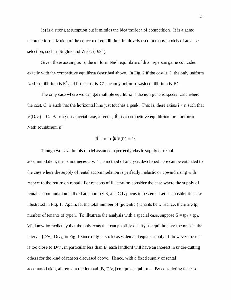
(b) is a strong assumption but it mimics the idea the idea of competition. It is a game

theoretic formalization of the concept of equilibrium intuitively used in many models of adverse

selection, such as Stiglitz and Weiss (1981).

Given these assumptions, the uniform Nash equilibria of this m-person game coincides

exactly with the competitive equilibria described above. In Fig. 2 if the cost is C, the only uniform

Nash equilibrium is R* and if the cost is ′C the only uniform Nash equilibrium is ′R .

The only case where we can get multiple equilibria is the non-generic special case where

the cost, C, is such that the horizontal line just touches a peak. That is, there exists i < n such that

V(D/vi) = C. Barring this special case, a rental, ~R , is a competitive equilibrium or a uniform

Nash equilibrium if

~R = min { }C)R(VR = .

Though we have in this model assumed a perfectly elastic supply of rental

accommodation, this is not necessary. The method of analysis developed here can be extended to

the case where the supply of rental accommodation is perfectly inelastic or upward rising with

respect to the return on rental. For reasons of illustration consider the case where the supply of

rental accommodation is fixed at a number S, and C happens to be zero. Let us consider the case

illustrated in Fig. 1. Again, let the total number of (potential) tenants be t. Hence, there are tpi

number of tenants of type i. To illustrate the analysis with a special case, suppose S = tp2 + tp3.

We know immediately that the only rents that can possibly qualify as equilibria are the ones in the

interval [D/v1, D/v2] in Fig. 1 since only in such cases demand equals supply. If however the rent

is too close to D/v1, in particular less than B, each landlord will have an interest in under-cutting

others for the kind of reason discussed above. Hence, with a fixed supply of rental

accommodation, all rents in the interval [B, D/v2] comprise equilibria. By considering the case

22

where { }t),pp(t,tpS 323 +≠ we can create equilibria where markets do not clear but this happens

in the special sense of tenants, who are indifferent between leasing an apartment in the rent

controlled area and the outside option, being excluded from the rent controlled sector.

IV. Inflation and Rents

Our model can be used to derive an interesting testable proposition concerning the relation

between inflation rates and rents in rent-controlled areas. The analysis however turn out to be

more complex than seems at first sight.

It is intuitively obvious that as the rate of inflation rises, (1) the inefficiencies of a rent-

controlled regime become more acute and (2) the long-stayers become more unattractive as

tenants from the point of view of the landlords than the short-stayers. (1) and (2) are technical

results; we derive these formally in Lemma 4 and Lemma 5, respectively. It is an implication of

these two lemmas that a higher inflation rate will result in a higher real rental rate for starting

tenants. Roughly speaking, the logic behind this proposition is that as inflation picks up, the

distortions created by tenancy rent control get exacerbated; the return earned by landlords drops;

and the market responds by causing rents to rise. This may well result in more tenants being

excluded from the rent-controlled market. In a country like India where the entire urban rental

market is controlled, this means more tenants will be excluded from the urban rental market

altogether.

Let us postpone further discussion until after the formal results are derived.

Note that in our model, a rise in the inflation rate simply means a fall in β , with zero

inflation being equivalent to β = 1. Throughout the following analysis we will assume 1≤β , that

23

is, we exclude the case of negative inflation. To make explicit the dependence of returns on the

rate of inflation, we will here write iv and )i(v as )(v i β and )(v )i( β , respectively.

Lemma 4 If β′ < β , then )(v )i( β′ < )(v )i( β .

Lemma 5 If β′ < β , then)(v

)(v

)(v

)(v

i

)i(

i

)i(

β

β<

β′

β′.

Using the two lemmas it is now possible to derive a testable proposition concerning the

relation between inflation and rent. There is no reason to believe that inflation alters the outside

options of agents in any systematic way. So we will take it to be neutral. Hence D and C remain

unchanged as the inflation rate changes. Let us also work here with the assumption of 'free entry'

of landlords, though that can be altered along the lines of analysis in the last part of Section III.

Let us see what happens to the V(R) curve as the rate of inflation rises that is, β changes

to β′ , which is less than β . From Lemma 1 we know that the ray Rv(i) will now be flatter for

every i.

Next consider each peak of the V(R) line, for instance, the peak at 2v/D in Fig. 1.

Clearly, the height of that peak is given by 2)2( v/Dv . From Lemma 5 we know that as inflation

increases (that is, β drops) this peak must get lower. This is, of course, true for every peak.

From the analysis in the previous section we know that the equilibrium point on the V(R)

curve must be at a point where the horizontal line at height C first hits the V(R) curve from the

left. From observations in the above two paragraphs we know that if the inflation rate increases

the V(R) curve will shift right with the new peaks no higher than before. It follows that the

equilibrium monthly rent, R, will rise. Since the equilibrium is the real rent faced by a starting

tenant, what we have just established is the proposition that, as the inflation rate rises, the real

rent for new leases goes up in economies in which there is tenancy rent control.

24

It is also easy to see that if the rise in inflation is sufficient the rise in the real rental can be

so sharp as to exclude a whole class of tenants who were earlier leasing apartments from the

rental market. This is not surprising at all because the inefficiency of tenancy rent control gets

more acute as the inflation rate rises.

V. Endogenous Quit Decisions

There are several directions in which one can modify and extend the above model. We

will in this section consider one involving the endogenization of the tenant’s type. It is true that

some people are inherently prone to moving and some have transferable jobs. But no matter what

the inherent penchants, people do modify their behavior depending on the conditions in the rental

market. If inflation is very high and a rent-control order holds the nominal rent constant for

sitting tenants, inherently peripatetic individuals may try to change their ways and stay put in one

place, and some people with transferable jobs may quit such jobs. In this section we shall try to

show that the endogenization of tenant types can generate some very interesting results, including

the generic possibility of multiple equilibria. Moreover, the removal of rent control can result in a

uniform lowering of rents.

Let us consider the case where all tenants are innately identical but they can choose to be

one of two types: 1 and 2. The assumption of ex ante identity is inessential and is made for ease

of explanation. Type i changes his apartment every ti months where t1 < t2. In other words, a

tenant chooses to be a short-stayer or a long-stayer. Again, for reasons of simplicity, let us

assume t2 = ∞ . In other words a potential tenant has to decide whether to be a short-stayer or

settle down permanently in a rented apartment. Let us see what happens if we have the kind of

tenancy rent control discussed in the previous section.

25

Consider alternative life strategies for the tenant. If a tenant decides on a career path in

which he moves to take up a better job, wherever such opportunities arise, he will be a short

stayer. Let his expected life-time wage-income in this case be W1. If alternatively he chooses a

life where he stays in one place and takes up whatever job he gets in the vicinity, he is a long

stayer and his expected life-time wage-income is W2. We assume W1>W2.

Suppose the market rent is R. A person who decides to be a tenant will choose to be a

short stayer if and only if [ ] [ ]W W v v R1 2 1 2− ≥ − . By Lemma 1, we know that the right-hand

term is positive. Hence, there exists a critical rent size, R , such that if R R≤ , tenants prefer

being of type 1 and if R> R , tenants prefer to be of type 2. Clearly,

RW W

v v≡

−−

1 2

1 2(7)

Let us, as in the end of section III, describe the outcome of the rental market by thinking

of this as a game among the m landlords. As before m > t, where t is the number of potential

tenants. For simplicity assume D is very high; so the potential tenants always choose to be

tenants. A tenant’s crucial decision now pertains to what type he will be. If all landlords charge

the same rent, R, each tenant’s choice has already been described. If R R≤ , each tenant chooses

to be of type 1. Otherwise he is of type 2.

Let us denote this decision by the function T:[ ) { }0 1 2, ,∞ → . T(R)=1 if and only if

R R≤ . Thus T(R) tells us what type the tenants will be, if there is only one rent, R, prevailing in

the market. Now, consider the case where, with all the landlords charging R, one landlord

deviates to ′R . What can the deviant landlord expect? As in section III, we assume that if

′R >R, she expects to find no tenants. If ′R <R, tenants will of course come to her, but the

question is what life-style will the tenant choose: short-staying or long-staying? It seems to us,

26

and this is what we will assume, that all tenants will be of type T(R) - even the tenant who rents at

rate ′R from the deviant landlord. More formally, in the language of games used at the end of

section III, we assume: (c) If t landlords enter the rental market and all but one of them charges a

rent of R and one landlord charges a rent ′R <R, then the tenants attracted by the deviant landlord

will be of type T(R).

This assumption seems to be intuitively very reasonable. Suppose you live in a city with a

tenancy rent control law in which every landlord, except one, charges a very high rent. The one

exception is your landlord who charges a low rent of ′R . Suppose if every landlord charged ′R

you would have adopted the short-staying life style (involving moving every time you got a better

job). What will you do when only your landlord charges ′R ? There seems little rational

motivation for you to adopt the short-staying life-style. In fact, since you know that higher rents

exist everywhere else, you will have an extra reason to stay put where you are.

This assumption is crucial to our model and it is worth clarifying that it is based on

intuition, which is external to our model. We, however, believe that it is a tenable assumption, and

hope that future work will be able to derive this postulate (c), from more basic axioms.

Fig. 3 considers the case in which all landlords charge the same rent R and the thick line

shows each landlord’s expected life-time rental income, V(R). Note that if

( ) ( )R R W W v v≤ ≡ − −1 2 1 2 , all tenants are of type 1 and if R> R , all tenants are of type 2.

27

Fig. 3: Equilibria with Endogenous Types

Now suppose (as in section III) a landlord’s cost of leasing out an apartment is C (as

shown in the figure). To fix our attention on the interesting case we consider one where the

horizontal line at C intersects V(R) more than once (at rents RL and RH). Unlike in section III,

here both RL and RH constitute competitive equilibria or, equivalently, uniform Nash equilibria. It

is obvious that RL is an equilibrium. So consider the case where the market rent is RH.

Landlords’ profits are zero, but it seems, at first sight, that an individual landlord can do better by

charging a lower rent--anything between RL and R . Suppose one landlord does so and charges

R R RL∈( , ] . She will have no problem getting a tenant of course. However the tenant who

moves in will not behave like a type 1 tenant, because if he gives up this tenancy there is no

Rv1

Rv2

V(R)

C

Monthly

Rent, RRRRL RH

28

reason for him to expect that he will again find an apartment for rent R. Hence, the deviating

landlord’s expected profit will be Rv2-C. This is non-positive for R R RL∈ ( , ] . So no one

benefits from deviating from RH, which is a competitive equilibrium. For a formal game-theoretic

argument we have to merely cite assumption (c) above to explain why it does not pay to undercut.

The argument that explains the possibility of multiple equilibria given tenancy rent control

is based on the assumption that there are limits to the number of apartments a single landlord can

offer (for simplicity assumed to be one in this paper). If a landlord could under cut RH by offering

( ]′ ∈R R RL , and supply a large number of apartments at that rent, she may be able to cause

tenants to alter their life’s strategy from being long-stayers to short-stayers. In other words (c)

would then no longer hold, and so RH would cease to be a uniform Nash equilibrium. But in any

metropolitan city it does seem reasonable to assume that no single landlord can cause such a large

infusion of apartments as to induce tenants to alter their life strategy.

Finally, if there is no rent control, clearly then RH will cease to be an equilibrium, because

landlords can write type-contingent contracts, So a landlord can deviate to a rent such as R and

make it contractual on the tenant quitting after t1 periods. It is easy to see that the only

equilibrium is at RL in Fig. 3.

The upshot is that, under tenancy rent control, both RH and RL are equilibria, whereas

under the free contract system only RL is. Suppose rent control is in effect and it is the bad

equilibrium, i.e. RH, that prevails. In comparison to this, no-rent-control is not only Pareto

efficient but it is Pareto dominant. The removal of rent control will result in all rents going down.

VI. Extensions: Turnover Costs, Signals and Identity

29

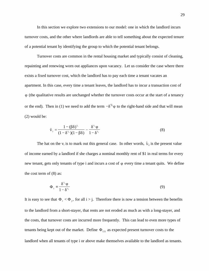
In this section we explore two extensions to our model: one in which the landlord incurs

turnover costs, and the other where landlords are able to tell something about the expected tenure

of a potential tenant by identifying the group to which the potential tenant belongs.

Turnover costs are common in the rental housing market and typically consist of cleaning,

repainting and renewing worn out appliances upon vacancy. Let us consider the case where there

exists a fixed turnover cost, which the landlord has to pay each time a tenant vacates an

apartment. In this case, every time a tenant leaves, the landlord has to incur a transaction cost of

φ (the qualitative results are unchanged whether the turnover costs occur at the start of a tenancy

or the end). Then in (1) we need to add the term −δ t i φ to the right-hand side and that will mean

(2) would be:

$( )

( )( )v i

t

t

t

t

i

i

i

i=

−− −

−−

1

1 1 1

βδδ βδ

δ φδ

(8)

The hat on the vi is to mark out this general case. In other words, ̂ v i is the present value

of income earned by a landlord if she charges a nominal monthly rent of $1 in real terms for every

new tenant, gets only tenants of type i and incurs a cost of φ every time a tenant quits. We define

the cost term of (8) as:

Φ i

t

t

i

i≡

−δ φ

δ1(9)

It is easy to see that Φ Φi j< , for all i > j. Therefore there is now a tension between the benefits

to the landlord from a short-stayer, that rents are not eroded as much as with a long-stayer, and

the costs, that turnover costs are incurred more frequently. This can lead to even more types of

tenants being kept out of the market. Define Φ ( )i as expected present turnover costs to the

landlord when all tenants of type i or above make themselves available to the landlord as tenants.

30

We can then write $ ( )v i as v(i) - Φ ( )i . If the rent is R and only tenants of type i and higher seek

tenancy, the landlord’s present value of income from leasing out one apartment is given by Rv(i) -

)i(Φ . This follows from (6), (9) and (13). It is now easy to see that with this specification it is no

longer generally true that if i < j, $ $( ) ( )v vi j> , and so from the landlord’s point of view the shortest

stayers are no longer necessarily the ideal tenants.

The tension between the desirability of oft-reset rents and undesirability of frequent

turnover costs can potentially alter the equilibrium from section III. Shorter stayers are likely to

be excluded from the rental market by landlords who want to avoid frequent turnover costs. They

accomplish this by setting rents high enough so that short-staying tenants exit the market.

Therefore turnover costs can lead to the exclusion of tenant types that would not have been

excluded in the absence of these costs.

In reality tenants are not as faceless as assumed in the model. People differ by race, age,

profession, nationality, and so on. Some of these may give a potential landlord a hint of how long

or short-stayer the tenant is likely to be. A person of a different nationality with a temporary visa

cannot be a long-stayer. Landlords may trust people of a certain age group or a certain race

more. In that case, at the time of leasing they can ask such tenants how long they plan to stay and

put greater trust in the answer than they would with other kinds of tenants. Landlords may also

believe that certain groups of tenants are more likely to leave when asked to do so. They will

then prefer tenants belonging to such a group.

The examples that we have given above are a mixed basket of inherent characteristics and

signals which a tenant can choose (e.g. his profession). For reasons of simplicity let us consider

the case of inherent characteristics. Suppose people belong to several different races, A, B, C, …

The expected length of stay of a tenant differs depending on which type one is and this is known

31

to landlords. So though, within each category, there are short-stayers and long-stayers, on

average A may be the shortest stayer; followed by B, C and so on. In such a market what we will

expect to see is a variety of rents. These will be contingent on the tenant’s race.

Thus, our model predicts that people in a profession which is known to involve transfer

and moving, or belonging to some identifiable group that is known to be footloose, will be found

paying a lower rent than those who are known to sink roots in one place and settle down.

VII. Conclusion

Rent control laws have been enacted in many countries around the world, making them

one of the most popular public policy prescriptions among metropolitan governments.

Unfortunately, knowledge of the effects of tenancy rent control (which is one of the most

pervasive forms of rent control) is inadequate, especially in the context of positive inflation. This

paper constructed a model of tenancy rent control and showed that this kind of rent control

system, with asymmetric information and exogenously given tenant types (the ‘type’ of a tenant

being identified in terms of how long a tenant expects to stay in the same apartment), lead to

outcomes that are Pareto sub-optimal. Free contracting, however, allows the agents in this model

to overcome the asymmetric information problem. The paper then studied a model in which how

long a tenant stays in one place is decided by the tenant on the basis of market signals. This

captures the fact that many agents make lifestyle choices depending on the conditions of the rental

housing market. Endogenizing the tenant’s type gives rise to the possibility of multiple equilibria

in our model. Removal of rent control laws can not only increase efficiency in the rental market,

but can also lead to a general lowering of rents, making all tenants better off.

A number of empirical implications arise from our model. Since landlords cannot write

departure date contingent contracts or have a rent escalation clause included in the contract, the

32

landlord must set initial rents higher to compensate for the erosion of real rents suffered during

occupancy. This should lead to across-the-board higher rents in rent-controlled apartments that

are being offered on the market (vacant apartments) than comparable offerings in non rent

controlled cities (as found in Nagy, 1997). One would also expect to find evidence of a tenure

discount in rent controlled cities (as in Nagy, 1997, and Börsch-Supan, 1986), where tenants who

have rented the same apartment for many years pay considerably less in rent than do tenants who

have only just recently taken possession of an apartment. 10 Some recent research (see Olsen,

1990) suggests that the construction of new housing need not be any less frequent in a rent

controlled city. However, in our basic model, as certain types are excluded from the rental

housing market, the supply of rental housing in the rent controlled market is likely to fall. In

addition, if increased inflation were severe enough to cause the exclusion of even more types (as

in section IV), then the supply of rental housing would fall as well.

An important implication of the model is that rent control might decrease the mobility of

the labor force. As sitting tenants are reluctant to move from a rent-controlled apartment, they

are less likely to accept a higher paying job in another city. Therefore, empirically, we would

expect to find that the average tenure of renters is higher in rent-controlled cities (as in Nagy,

1997, and, to some extent, in Olsen, 1990), and that rent control reduces tenant mobility (as in

Nagy, 1995, and Ault, et al., 1994). In fact, Nagy (1997) presents empirical findings that are

directly in line with our model. He studies New York City apartments under the post-1974 rent

stabilization scheme and finds that in 1981, rent stabilized apartments had higher initial rents than

non-stabilized apartments. Six years later, for those tenants who remained in the same apartment

in both sectors, those in the stabilized sector paid lower rents. In addition, tenants in the

10 Tenure discounts may also occur in non-rent controlled areas as well, however the empirical evidence is mixed.

33

stabilized sector had longer tenure durations than tenants in the non-stabilized sector. Thus, the

received empirical evidence generally supports these hypotheses, drawing a picture remarkably

similar to the one that is implied by our model, but the scarcity of detailed empirical evidence

suggests that there is still work to be done in this area.

Our model also drew attention to some systematic relations between rates of inflation and

rental rates for property under tenancy rent control. These are testable propositions but evidence

on this is hard to come by. It is hoped that our model, by clarifying the theoretical link between

inflation and rent, will prompt researchers to collect and empirically verify the claims that arise

from this theory.

From the above set of results, it is easy to get the idea that the optimal policy solution is to

free the rental housing market of all government restrictions. We caution the reader from

extending this logic too far, however. As we discuss earlier in the paper, free contracting in the

rental housing market, in the sense that we use it, does entail certain important responsibilities on

the part of government. The government provides the framework in which contracts are

enforced, and though in our model the absence of rent control was associated with a system of

free contract, there will in reality be three important kinds of limits on the range of contracts

allowed. First, since every society considers certain kinds of activities illegal, a contract that

specifies the use of some illegal activity would naturally not be recognized even of both parties

voluntarily agree to it. A contract which entails the landlord killing a tenant who fails to pay the

rent would belong to this category. Second, a contract which adversely affects an uninvolved

‘third party’ (that is, someone who is not a signatory to the contract) would be considered illegal.

Finally, what one has to keep in mind is that, in this age of lawyers, contracts can soon become so

See Guasch and Marshall (1987).

34

complicated that it becomes virtually impossible for the signatories to fully understand what

exactly they are agreeing to. In such a scenario, the more savvy can ‘trap’ the others into

transactions that they would not have got into if they understood the full ramifications of the

contract. To prevent this from happening, a practical response is to set some broad limits to the

range of permitted contracts. To the extent that rent controls are themselves partly the

consequence of a well-meaning attempt to restrict the range of contracts, one has to exercise

commonsense when limiting the terrain of possible contracts. What our model suggests is that the

class of possible contracts should include rent escalation clauses, tenancy termination clauses and

in general, contracts involving terms which are departure date contingent. This freedom of choice

allows tenants and landlords to overcome the asymmetric information problem and reaches not

only Pareto efficiency but may result in across-the-board lower housing rentals than what occurs

in the presence of rent control.

35

Appendix A: Proofs of Lemmas

Proof of Lemma 1 We shall, without loss of generality, assume that tj = ti+1. Let vjk be the

present value of rents earned by a landlord whose first k tenants are of type i and all others of type

j. (Hence, vj0 = vj )

We first show that vj1 > vj. Clearly,

v vjt t

ji i1 2 11= + + + + +−βδ βδ βδ δ( ) ( )L (11)

Since tj = ti+1 , and given (3) and (1), we have

v vj j1 − = δ βδ δt

jt t

ji i iv v− − +( ) 1

= [ ]δ δ βtj

ti iv( )1 − −

= ( )11

− −−

δ δ

βδ

tj

t

i

i

v

It is easy to see v j

t i

>−

βδ1

. (12)

The right-hand term is the present value of the stream [ ]β βt ti i, , L , while vj is the present

value of the sequence [ ]1 1 12 2, , , , , , , , , , ,β β β β β βL L Lt ti i The latter

sequence dominates the former, term by term. Hence, (12) is true, and, therefore, vj1 > vj.

It is easy to check, vjk > vj

k-1, ∀k , and that limk j

kiv v

→∞= . It follows that vi > vj. n

Proof of Lemma 2 Note that, for all k,

v vkt t

kk k= + + + + +−1 2 1βδ βδ βδ δ( ) ( )L

or

1 12 1+ + + + = −−βδ βδ βδ δ( ) ( ) ( )L t tk

k k v

36

Substituting this in (4), we get

v

p

p

v

p

p

i

k

jj i

nk i

ntk

k

k

jj i

ntk

k i

n

( )

( )

=

−

−

=

=

=

=

∑∑

∑∑

1

1

δ

δ

or v

p v

p pi

ktk

kk i

n

j ktk

k i

n

j i

n( )

( )

=−

−

=

==

∑

∑∑

1 δ

δ(13)

It is worth noting that if the term vk was not there on the right-hand side of (13) then the right-

hand side would be equal to 1. Hence, v(i) is clearly a weighted average of vi, vi+1, ..., and vn. It is

also evident that if j > i, v(i) is gotten from v(j) by redistributing some of the weights away from vj,

... , vn to vi, ... , vj-1. Since, for all k < j, vk > vj (by Lemma 1), it follows that v(i) > v(j). n

Proof of Lemma 4 From (1) it is obvious that

[ ] 1t2k

t kk )()(1)(v1 −βδ++βδ+βδ+=βδ− L (14)

Writing the expression for v(i) derived in the proof of Lemma 2, with the dependence on β made

explicit, we have:

37

[ ]

∑∑

∑∑

=

=

=

=

δ

−

βδ−

=β

n

ik

tn

ijj

k

kt

n

ikn

ijj

k

)i(

k

k

p

p1

)(v1

p

p

)(v (15)

By inspecting (14) it is obvious that β′ < β implies )(v k β′ < )(v k β , for all k. From (15) it

follows that )(v )i( β′ < )(v )i( β . n

Proof of Lemma 5 Assume β′ < β . From (15) it is clear that if

)(v

)(v

)(v

)(v

i

k

i

k

ββ

<β′β′

, for all k > i, (16)

then the proof of the lemma is complete. The remainder of this proof is therefore devoted to

establishing (16).

Let k > i. Define ik ttm −≡ . Clearly m ≥ 1. From (2) it follows that

i

i

i

i

i

i

t

mt

t

mt

mt

t

i

k

)(1

)(1Z

)(1

)(1

1

1

)(v

)(v

βδ−βδ−

⋅≡βδ−

βδ−⋅

δ−δ−

=ββ ++

+

By differentiating the right-hand term with respect to β it can be checked that as β falls, the term

becomes smaller. Hence, (16) is proved. n

38

REFERENCES

Akerlof, G. (1970). ‘The Market for ‘Lemons’: Quality Uncertainty and the Market Mechanism.’

Quarterly Journal of Economics, vol. 84, pp. 488-500.

Arnott, R. (1995). ‘Time for Revisionism on Rent Control?’ Journal of Economic Perspectives,

vol. 9, pp. 99-120.

Ault, R.W., Jackson, J.D., and Saba, R.P. (1994). ‘The Effect of Long-Term Rent Control on

Tenant Mobility.’ Journal of Urban Economics, vol. 35, pp. 140-158.

Basu, K. (1989). ‘Technological Stagnation, Tenurial Laws, and Adverse Selection.’ American

Economic Review, vol. 79, pp. 251-255.

Börsch-Supan, A. (1986). ‘On the West German Tenants’ Protection Legislation.’ Journal of

Institutional and Theoretical Economics, vol. 142, pp. 380-404.

Cinque, R.A. (1997) “Non-Rent Protections Under Rent Control and Rent Stabilization.” New

York Law Journal.

Drier, P. (1997). ‘Rent Deregulation in California and Massachusetts: Politics, Policy, and

Impacts.’ Paper presented at the ‘Housing ‘97’ Conference at New York University, May

14.

Epple, D. (1998). ‘Rent Control with Reputation: Theory and Evidence.’ Regional Science and

Urban Economics, vol. 28, pp. 679-710.

Fallis, G. (1988) ‘Rent Control: The Citizen, the Market and the State.’ Journal of Real Estate

Finance and Economics, vol. 1, pp. 309-320.

Frankena, M. (1975). ‘Alternative Models of Rent Control.’ Urban Studies, vol. 12, pp. 303-308.

Guasch, J.L., and Marshall, R.C. (1987). ‘A Theoretical and Empirical Analysis of the Length of

Residency Discount in the Rental Housing Market.’ Journal of Urban Economics, vol.

22, pp. 291-311.

Hubert, F. (1995). ‘Contracting with Costly Tenants.’ Regional Science and Urban Economics,

vol. 25, pp. 631-654.

Hubert, F. (1996). ‘Rental Contracts, Endogenous Turnover and Rent Volatility.’

Diskussionbeiträge des Fachbereichs Wirtschaftswissenschaft der Freien Universität

Berlin.

39

Jarett, S, and McKee, M. (1997). Rent Regulation in New York City: A Briefing Book. New

York: Community Training and Resource Center.

Linneman, P. (1985). ‘The Effect of Rent Control on the Distribution of Income among New

York City Renters.’ Journal of Urban Economics, vol. 22,pp. 14-34.

Mas-Colell, A, Whinston, M.D., and Green, J.R. (1995). Microeconomic Theory. Oxford: Oxford

University Press.

Nagy, J. (1997). ‘Do Vacancy Decontrol Provisions Undo Rent Control?’ Journal of Urban

Economics, vol. 42, pp. 64-78.

Nagy, J. (1995). ‘Increased Duration and Sample Attrition in New York City's Rent Controlled

Sector.’ Journal of Urban Economics, vol. 38, pp. 127-137.

Olsen, E.O. (1990). ‘What is Known About the Effects of Rent Controls?’ Consulting Report for

U.S. Department of Housing and Urban Development, Contract Number NA 90-7272,

(September).

Raymon, N. (1983). ‘Price Ceilings in Competitive Markets with Variable Quality.’ Journal of

Public Economics, vol. 22, pp. 257-264.

Smith, L.B., Rosen, K.T., and Fallis, G. (1988). ‘Recent Developments in Economic Models of

Housing Markets.’ Journal of Economic Literature, vol. 26, pp. 29-64.

Stiglitz, J.E. and Weiss, A. (1981). ‘Credit Rationing in Markets with Imperfect Information.’

American Economic Review, vol. 71, pp. 393-410.

Sweeney, J.L. (1974). ‘Quality, Commodity Hierarchies, and Housing Markets.’ Econometrica,

vol. 42, pp. 147-167.