The Economic Consequences of Cognitive Dissonance By George A. Akerlof and William T. Dickens

Presented by Lucy Chang, Allison Jaros, Erin Lett, and Morgan Lucas (Coase Team)

April 3, 2012

I. Introduction

In the 1950’s a radical group led by a woman named Marian Keech believed that the

world would end in a great flood on December 21, 1954. Mrs. Keech told believers that they

would survive this flood by being picked up in a flying saucer. In response, many believers quit

their jobs and sold their possessions. A young psychologist named Leon Festinger infiltrated the

group to see what would happen when December 21 passed and the prophesy was unfulfilled.

Festinger predicted that, while those who had kept their property would lose faith in Mrs. Keech,

those who had invested more heavily in the truth of the prophesy would increase their degree of

belief. When there was no flood and the space ship failed to appear, Mrs. Keech told her

followers that their faith in her had saved the world. Those who had sacrificed their jobs and

possessions called radio stations and took to the streets to try and convert others, while those

who had not invested as much in Mrs. Keech’s prophesy lost their faith and abandoned the

group.1 Festinger’s prediction had been correct. In 1957, Leon Festinger published his findings in

a book called “A Theory of Cognitive Dissonance.” In it, he explained that the reason he

observed these results was because of the uncomfortable feeling that comes from investing in

something or believing in something that turns out to be wrong. Because people prefer to think

of themselves as intelligent, it was easier for those who had invested heavily in Mrs. Keech’s

prophesy to believe more fervently than to admit that they had invested in a false prophesy.

Cognitive dissonance, which is formally defined as the discomfort that comes from

holding conflicting beliefs, can have implications for how people make decisions and evaluate

information. Akerlof and Dickens propose that cognitive dissonance can be incorporated into

economic models in a number of settings. In “The Economic Consequences of Cognitive

Dissonance” they propose a formal model in the setting of workplace safety. They emphasize

that it is important to consider the effects of cognitive dissonance because it can have important

implications that not only justify but also support the need policy intervention.

1 Elliot Arinson, Why It’s Hard to Admit Being Wrong, NPR News, July 20, 2007, available at

http://www.npr.org/templates/story/story.php?storyId=12125926.

II. Basic Premises and an Overview of the Model

The basic premise of Akerlof and Dickens’ model can be broken down into three

propositions. First, people have preferences over states of the world and over their beliefs about

those states. Second, people have a degree of control over their beliefs; they are “able to exercise

some choice about belief given available information,” and they can manipulate their beliefs by

drawing on information that is likely to confirm their favorable beliefs. Third, once chosen,

beliefs persist over time. Akerlof and Dickens demonstrate how psychological studies have

supported the idea the people act according to these premises in certain circumstances. They

assert that these three premises allow them to develop a model for how workers in hazardous

environments react to the dangers they face, and that these reactions cannot be incorporated into

Bayesian decision theory.

A. Psychological Evidence for Akerlof and Dickens’ Premises

The theory of cognitive consistency is a pillar of social psychology. Because people aim

to make their beliefs consistent with one another, they are “uncomfortable in maintaining two

seemingly contradictory ideas.” As illustrated in the example presented in the introduction, most

people like to view themselves as smart, nice people so they reject information that is

inconsistent with these beliefs. Therefore, Ms. Keech’s believers rejected the evidence that their

doomsday prediction had been wrong and accepted the belief that they had saved the world. A

number of other psychological studies support the theory of cognitive dissonance and the three

propositions Akerlof and Dickens use to describe it.

One of these studies involved betting at a horse race and it demonstrated how groups of

people with the same information can hold different beliefs that are consistent with natural

theories about their preferences. At a racetrack, interviewers asked people who had just placed a

bet on a horse and people who were just about to place a bet what they thought their odds on

winning would be. The responses indicated that those who had just placed their bets

systematically placed higher odds on their horse winning than those who had not yet placed their

bet. In the context of Akerlof and Dickens’ propositions: first, while people prefer to be correct,

they also prefer to believe that they are correct; second, people are able to control their beliefs –

those interviewed after placing bets believed that they had higher odds of winning than those

who were about to place bets; and third, those beliefs persist over time, so it would be expected

that those who had already placed bets would keep believing that they had higher odds of

winning.

B. Application in the Context of Workplace Safety

Akerlof and Dickens assert that they can apply their three propositions to the context of

workplace safety. They state that there is a great deal of evidence that workers in dangerous jobs

are often oblivious to the dangers they face. In terms of their propositions, workers prefer to

believe that their workplace is safe, so they make a choice about whether to believe it is safe and

their choice persists over time. Yet the important lesson, and the one that they seek to show

through their model, is that these choices over beliefs come at a cost, and that cost can have

important implications that ultimately justify policy intervention.

C. The Need for a New Model

Before presenting their model of workplace safety, Akerlof and Dickens are careful to

emphasize that cognitive dissonance cannot simply be incorporated through Bayesian decision

theory. The reason, they say, is that cognitive dissonance involves changes in beliefs in the

presence of no new and relevant information. In the horserace example, the systematic difference

in how betters viewed their odds of winning did not change because of new information; it

merely changed because those who already placed their bets had a stronger preference to hold

the belief that their bet was correct. After providing a basic overview of Bayesian decision

theory, it will be clear that cognitive dissonance generally cannot be represented under the

Bayesian approach.

In Bayesian decision theory, individuals are faced with a decision under uncertainty.

They have preferences and information that influence their estimates of each of the possible

outcomes. The basic idea behind Bayesian decision theory can be represented by a two period

model in which an individual in Econ 206 is trying to decide whether to attend a particular

group’s presentation. Presumably, the individual would like to attend the presentation if she

thinks that it will be interesting. Based on the quality of the past presentations, he knows that the

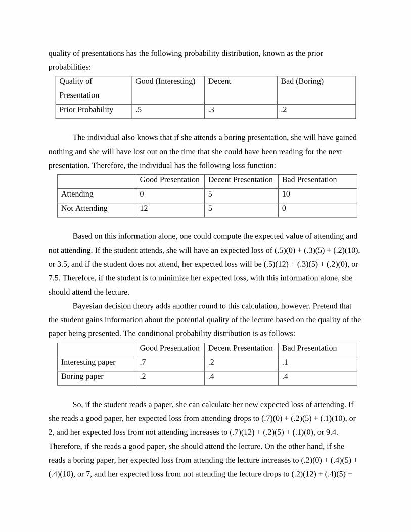
quality of presentations has the following probability distribution, known as the prior

probabilities:

Quality of

Presentation

Good (Interesting) Decent Bad (Boring)

Prior Probability .5 .3 .2

The individual also knows that if she attends a boring presentation, she will have gained

nothing and she will have lost out on the time that she could have been reading for the next

presentation. Therefore, the individual has the following loss function:

Good Presentation Decent Presentation Bad Presentation

Attending 0 5 10

Not Attending 12 5 0

Based on this information alone, one could compute the expected value of attending and

not attending. If the student attends, she will have an expected loss of (.5)(0) + (.3)(5) + (.2)(10),

or 3.5, and if the student does not attend, her expected loss will be (.5)(12) + (.3)(5) + (.2)(0), or

7.5. Therefore, if the student is to minimize her expected loss, with this information alone, she

should attend the lecture.

Bayesian decision theory adds another round to this calculation, however. Pretend that

the student gains information about the potential quality of the lecture based on the quality of the

paper being presented. The conditional probability distribution is as follows:

Good Presentation Decent Presentation Bad Presentation

Interesting paper .7 .2 .1

Boring paper .2 .4 .4

So, if the student reads a paper, she can calculate her new expected loss of attending. If

she reads a good paper, her expected loss from attending drops to (.7)(0) + (.2)(5) + (.1)(10), or

2, and her expected loss from not attending increases to (.7)(12) + (.2)(5) + (.1)(0), or 9.4.

Therefore, if she reads a good paper, she should attend the lecture. On the other hand, if she

reads a boring paper, her expected loss from attending the lecture increases to (.2)(0) + (.4)(5) +

(.4)(10), or 7, and her expected loss from not attending the lecture drops to (.2)(12) + (.4)(5) +

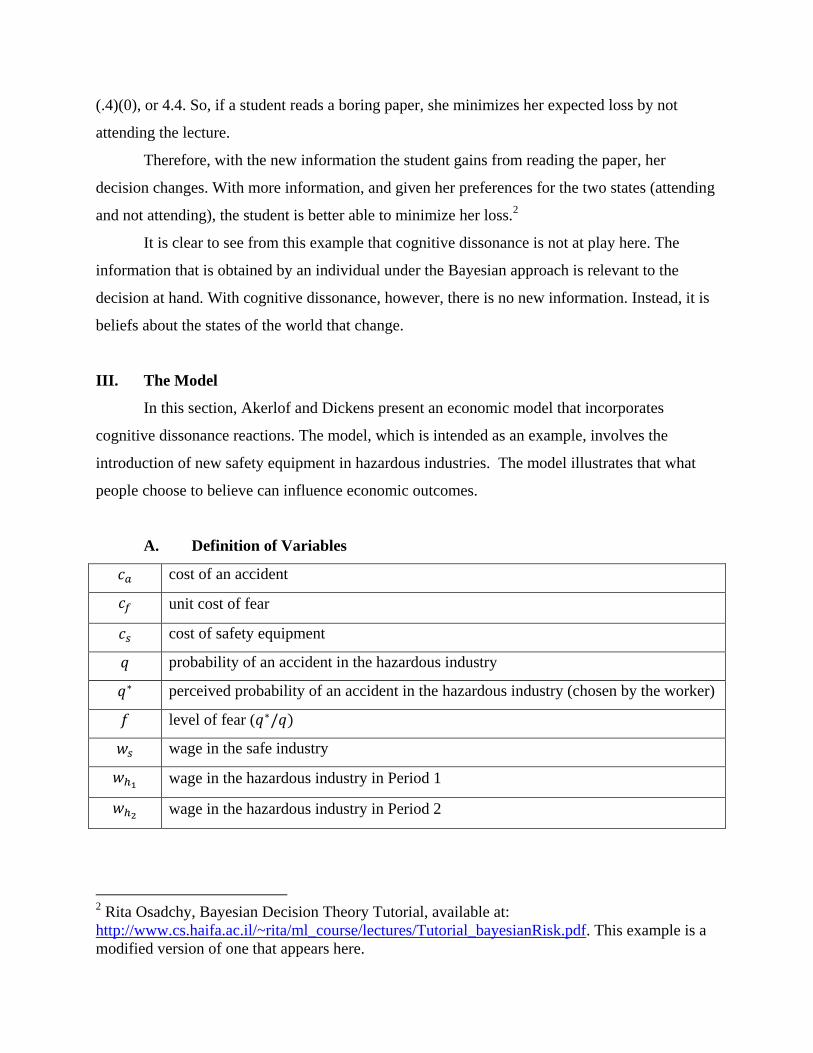
(.4)(0), or 4.4. So, if a student reads a boring paper, she minimizes her expected loss by not

attending the lecture.

Therefore, with the new information the student gains from reading the paper, her

decision changes. With more information, and given her preferences for the two states (attending

and not attending), the student is better able to minimize her loss.2

It is clear to see from this example that cognitive dissonance is not at play here. The

information that is obtained by an individual under the Bayesian approach is relevant to the

decision at hand. With cognitive dissonance, however, there is no new information. Instead, it is

beliefs about the states of the world that change.

III. The Model

In this section, Akerlof and Dickens present an economic model that incorporates

cognitive dissonance reactions. The model, which is intended as an example, involves the

introduction of new safety equipment in hazardous industries. The model illustrates that what

people choose to believe can influence economic outcomes.

A. Definition of Variables

cost of an accident

unit cost of fear

cost of safety equipment

probability of an accident in the hazardous industry

perceived probability of an accident in the hazardous industry (chosen by the worker)

level of fear (

wage in the safe industry

wage in the hazardous industry in Period 1

wage in the hazardous industry in Period 2

2 Rita Osadchy, Bayesian Decision Theory Tutorial, available at:

http://www.cs.haifa.ac.il/~rita/ml_course/lectures/Tutorial_bayesianRisk.pdf. This example is a

modified version of one that appears here.

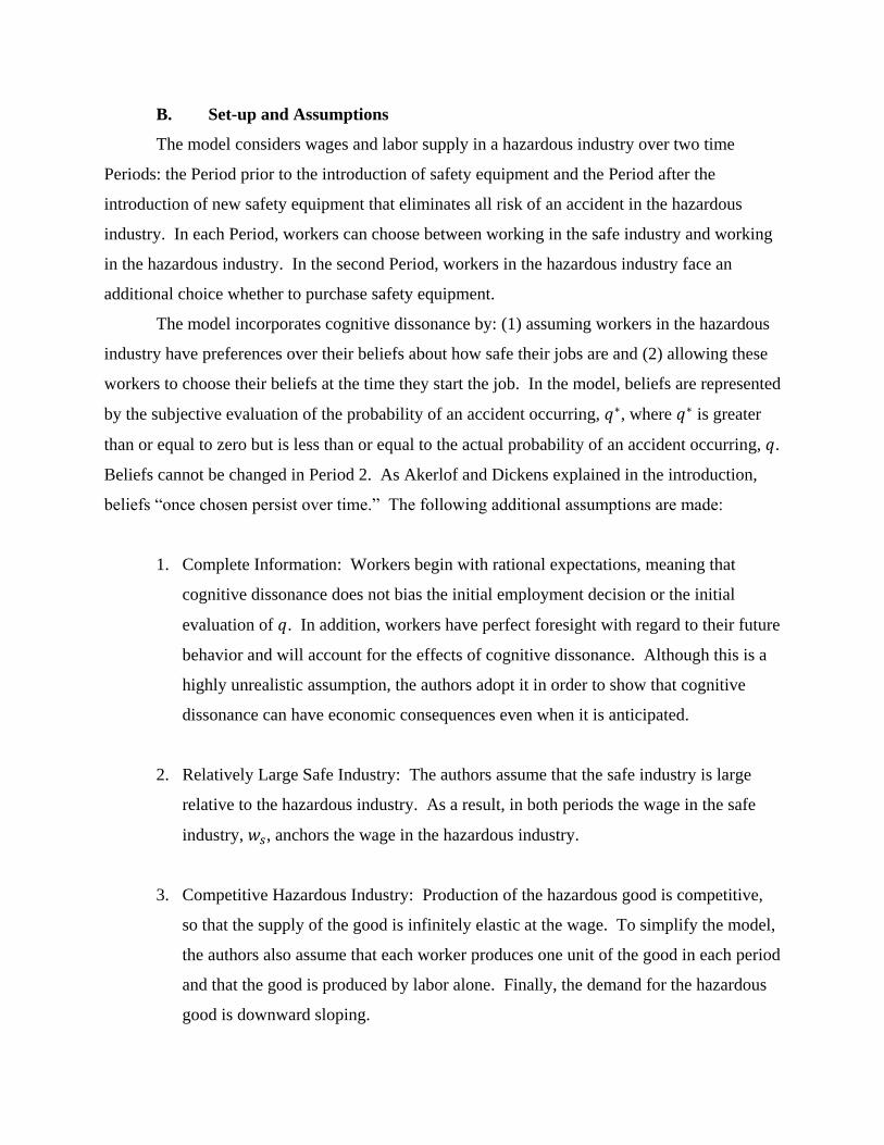
B. Set-up and Assumptions

The model considers wages and labor supply in a hazardous industry over two time

Periods: the Period prior to the introduction of safety equipment and the Period after the

introduction of new safety equipment that eliminates all risk of an accident in the hazardous

industry. In each Period, workers can choose between working in the safe industry and working

in the hazardous industry. In the second Period, workers in the hazardous industry face an

additional choice whether to purchase safety equipment.

The model incorporates cognitive dissonance by: (1) assuming workers in the hazardous

industry have preferences over their beliefs about how safe their jobs are and (2) allowing these

workers to choose their beliefs at the time they start the job. In the model, beliefs are represented

by the subjective evaluation of the probability of an accident occurring, , where is greater

than or equal to zero but is less than or equal to the actual probability of an accident occurring, .

Beliefs cannot be changed in Period 2. As Akerlof and Dickens explained in the introduction,

beliefs “once chosen persist over time.” The following additional assumptions are made:

1. Complete Information: Workers begin with rational expectations, meaning that

cognitive dissonance does not bias the initial employment decision or the initial

evaluation of . In addition, workers have perfect foresight with regard to their future

behavior and will account for the effects of cognitive dissonance. Although this is a

highly unrealistic assumption, the authors adopt it in order to show that cognitive

dissonance can have economic consequences even when it is anticipated.

2. Relatively Large Safe Industry: The authors assume that the safe industry is large

relative to the hazardous industry. As a result, in both periods the wage in the safe

industry, , anchors the wage in the hazardous industry.

3. Competitive Hazardous Industry: Production of the hazardous good is competitive,

so that the supply of the good is infinitely elastic at the wage. To simplify the model,

the authors also assume that each worker produces one unit of the good in each period

and that the good is produced by labor alone. Finally, the demand for the hazardous

good is downward sloping.

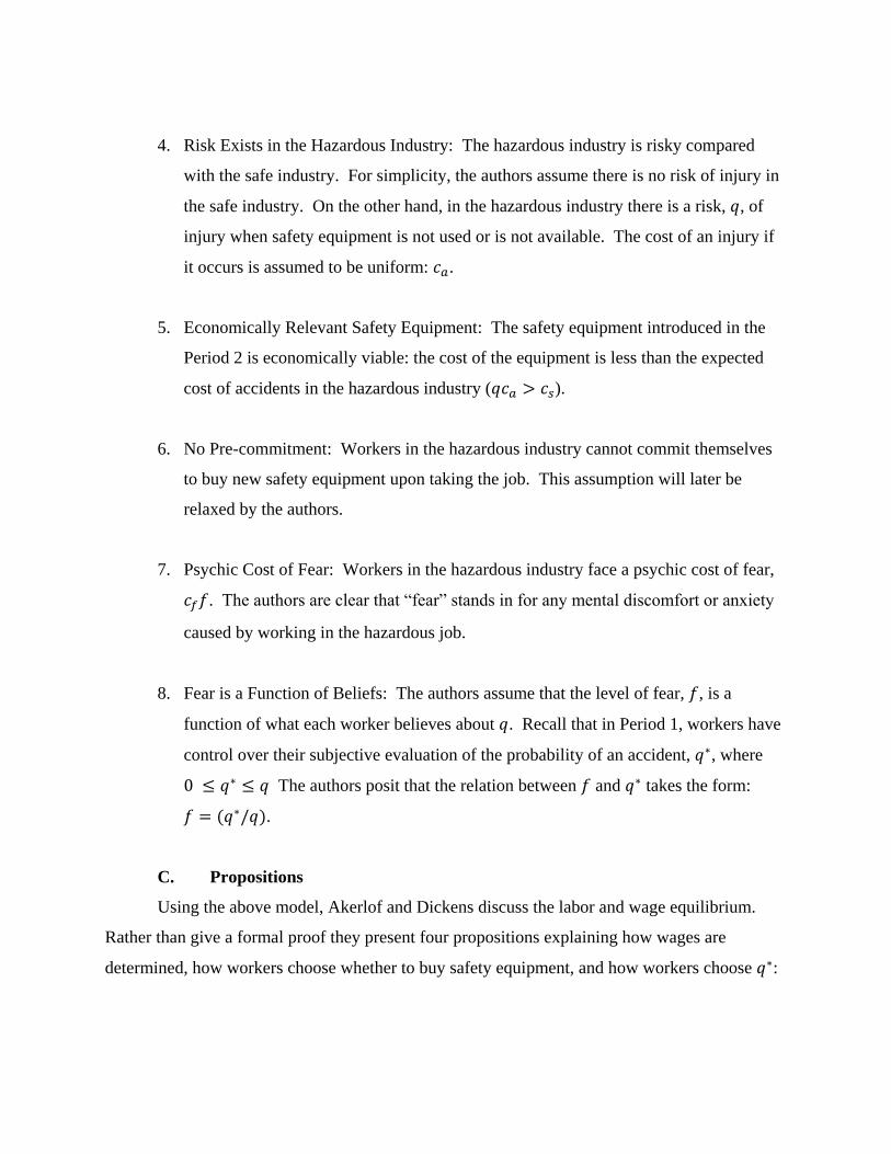
4. Risk Exists in the Hazardous Industry: The hazardous industry is risky compared

with the safe industry. For simplicity, the authors assume there is no risk of injury in

the safe industry. On the other hand, in the hazardous industry there is a risk, , of

injury when safety equipment is not used or is not available. The cost of an injury if

it occurs is assumed to be uniform: .

5. Economically Relevant Safety Equipment: The safety equipment introduced in the

Period 2 is economically viable: the cost of the equipment is less than the expected

cost of accidents in the hazardous industry ( ).

6. No Pre-commitment: Workers in the hazardous industry cannot commit themselves

to buy new safety equipment upon taking the job. This assumption will later be

relaxed by the authors.

7. Psychic Cost of Fear: Workers in the hazardous industry face a psychic cost of fear,

. The authors are clear that “fear” stands in for any mental discomfort or anxiety

caused by working in the hazardous job.

8. Fear is a Function of Beliefs: The authors assume that the level of fear, , is a

function of what each worker believes about . Recall that in Period 1, workers have

control over their subjective evaluation of the probability of an accident, , where

The authors posit that the relation between and takes the form:

.

C. Propositions

Using the above model, Akerlof and Dickens discuss the labor and wage equilibrium.

Rather than give a formal proof they present four propositions explaining how wages are

determined, how workers choose whether to buy safety equipment, and how workers choose :

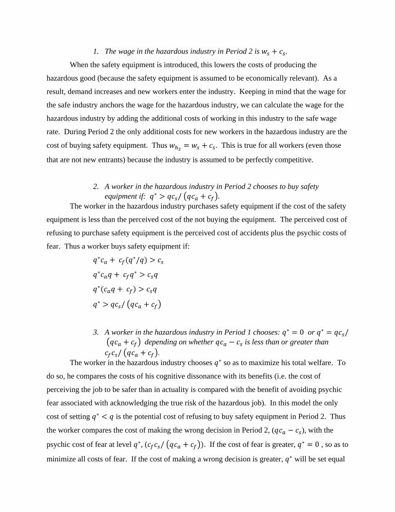
1. The wage in the hazardous industry in Period 2 is .

When the safety equipment is introduced, this lowers the costs of producing the

hazardous good (because the safety equipment is assumed to be economically relevant). As a

result, demand increases and new workers enter the industry. Keeping in mind that the wage for

the safe industry anchors the wage for the hazardous industry, we can calculate the wage for the

hazardous industry by adding the additional costs of working in this industry to the safe wage

rate. During Period 2 the only additional costs for new workers in the hazardous industry are the

cost of buying safety equipment. Thus . This is true for all workers (even those

that are not new entrants) because the industry is assumed to be perfectly competitive.

2. A worker in the hazardous industry in Period 2 chooses to buy safety

equipment if: .

The worker in the hazardous industry purchases safety equipment if the cost of the safety

equipment is less than the perceived cost of the not buying the equipment. The perceived cost of

refusing to purchase safety equipment is the perceived cost of accidents plus the psychic costs of

fear. Thus a worker buys safety equipment if:

3. A worker in the hazardous industry in Period 1 chooses: or depending on whether is less than or greater than

.

The worker in the hazardous industry chooses so as to maximize his total welfare. To

do so, he compares the costs of his cognitive dissonance with its benefits (i.e. the cost of

perceiving the job to be safer than in actuality is compared with the benefit of avoiding psychic

fear associated with acknowledging the true risk of the hazardous job). In this model the only

cost of setting is the potential cost of refusing to buy safety equipment in Period 2. Thus

the worker compares the cost of making the wrong decision in Period 2, ( ), with the

psychic cost of fear at level , ( . If the cost of fear is greater, , so as to

minimize all costs of fear. If the cost of making a wrong decision is greater, will be set equal

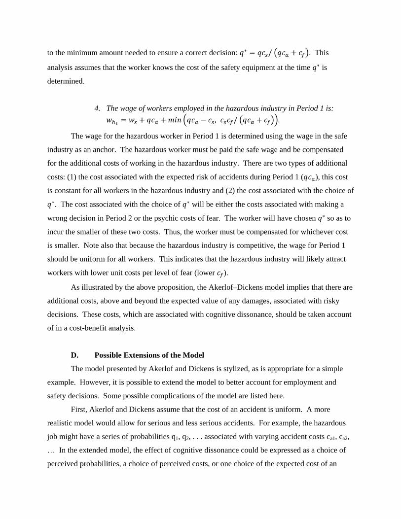
to the minimum amount needed to ensure a correct decision: . This

analysis assumes that the worker knows the cost of the safety equipment at the time is

determined.

4. The wage of workers employed in the hazardous industry in Period 1 is:

.

The wage for the hazardous worker in Period 1 is determined using the wage in the safe

industry as an anchor. The hazardous worker must be paid the safe wage and be compensated

for the additional costs of working in the hazardous industry. There are two types of additional

costs: (1) the cost associated with the expected risk of accidents during Period 1 ( ), this cost

is constant for all workers in the hazardous industry and (2) the cost associated with the choice of

. The cost associated with the choice of will be either the costs associated with making a

wrong decision in Period 2 or the psychic costs of fear. The worker will have chosen so as to

incur the smaller of these two costs. Thus, the worker must be compensated for whichever cost

is smaller. Note also that because the hazardous industry is competitive, the wage for Period 1

should be uniform for all workers. This indicates that the hazardous industry will likely attract

workers with lower unit costs per level of fear (lower ).

As illustrated by the above proposition, the Akerlof–Dickens model implies that there are

additional costs, above and beyond the expected value of any damages, associated with risky

decisions. These costs, which are associated with cognitive dissonance, should be taken account

of in a cost-benefit analysis.

D. Possible Extensions of the Model

The model presented by Akerlof and Dickens is stylized, as is appropriate for a simple

example. However, it is possible to extend the model to better account for employment and

safety decisions. Some possible complications of the model are listed here.

First, Akerlof and Dickens assume that the cost of an accident is uniform. A more

realistic model would allow for serious and less serious accidents. For example, the hazardous

job might have a series of probabilities q1, q2, . . . associated with varying accident costs ca1, ca2,

… In the extended model, the effect of cognitive dissonance could be expressed as a choice of

perceived probabilities, a choice of perceived costs, or one choice of the expected cost of an

accident during a given period. In other words, the model could potentially account for a set of

beliefs over states of the world. The current model only models the choice of belief about one

variable.

Second, Akerlof and Dickens do not discuss the length of the two periods (by stating that

one unit is produced during each period they seem to indicate that the periods are equal). The

model in the paper fails to account for time effects. For example, if the length of time before the

new safety equipment is introduced is very short, we might expect workers to be more likely to

set high enough to make a correct decision. Akerlof and Dickens also do not discuss whether

workers might discount future harm or benefit during the decision process. If they discount

future harm, they may not ask for sufficient compensation in Period 1 to fully compensate them

for the decision not to adopt safety equipment during Period 2.

Third, the model in the paper indicates that the wage in the hazardous industry will drop

with the introduction of new safety equipment. Yet, the phenomenon of cognitive dissonance

might suggest that workers in the hazardous industry are unlikely to accept a drop in wages.

Instead, they are likely to believe that they deserve the inflated wage despite the decrease in

production costs. The current model assumes new entrants will drive out previous employees in

this case—as new entrants will be willing to work for a lower wage. If the market is not

perfectly competitive or if wages are sticky, the model may not accurately predict the effects of

the introduction of new safety equipment.

Finally, Akerlof and Dickens assume the only negative consequence of reducing is

making the wrong decision concerning safety equipment. A more realistic model would

recognize that reducing may actually affect . So that the perception of risk causes workers to

be less careful, raising the likelihood of an accident. In other words, one consequence of

cognitive dissonance is that it can change the state of the world by changing how individuals

behave. Thus, errors caused by cognitive dissonance may be compounded over time.

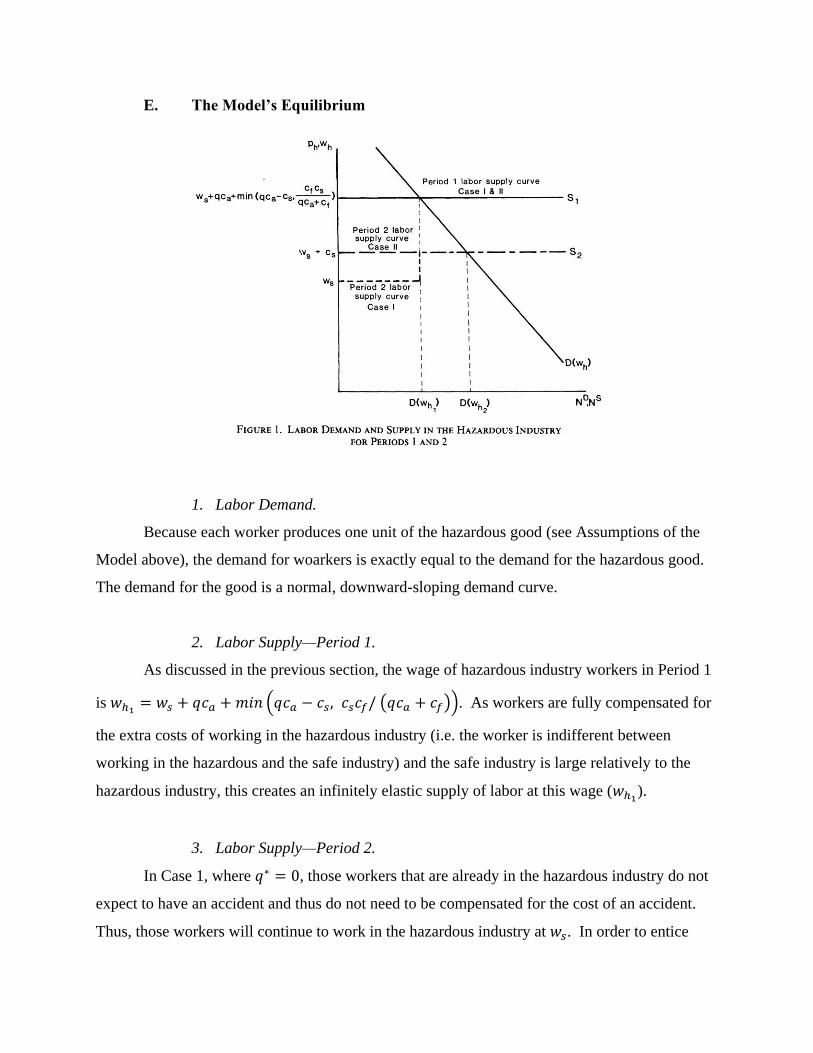
E. The Model’s Equilibrium

1. Labor Demand.

Because each worker produces one unit of the hazardous good (see Assumptions of the

Model above), the demand for woarkers is exactly equal to the demand for the hazardous good.

The demand for the good is a normal, downward-sloping demand curve.

2. Labor Supply—Period 1.

As discussed in the previous section, the wage of hazardous industry workers in Period 1

is . As workers are fully compensated for

the extra costs of working in the hazardous industry (i.e. the worker is indifferent between

working in the hazardous and the safe industry) and the safe industry is large relatively to the

hazardous industry, this creates an infinitely elastic supply of labor at this wage ( ).

3. Labor Supply—Period 2.

In Case 1, where , those workers that are already in the hazardous industry do not

expect to have an accident and thus do not need to be compensated for the cost of an accident.

Thus, those workers will continue to work in the hazardous industry at . In order to entice

labor to move from the safe industry to the hazardous industry in Period 2, these new workers

must be compensated for the cost of the safety equipment . At this point, the workers will be

indifferent between working in the safe industry and the hazardous industry, and the labor supply

curve will be infinitely elastic at .

In Case 2, where , workers already in the hazardous industry will

purchase safety equipment in Period 2 (see Proposition 3 above) and must be compensated for

this expenditure; thus . This is the same wage necessary to entice workers away from

the safe industry in Period 2. There is thus an infinitely elastic supply of labor at this wage level.

Because the model assumes that in order to make the safety equipment

economically relevant, the Period 2 wage is lower than the Period 1 wage in either Case 1 or

Case 2.

, which is always less than

Because , more labor will be demand in Period 2 than in Period 1 (i.e. the labor

demand curve will intercept the labor supply curve to the right of D( . This means that both

labor supply curves would intercept the labor demand curve where infinitely elastic at .

F. The Equilibrium Discussed

In equilibrium all workers have the same pecuniary and non-pecuniary income when

summed over the two periods:

- For workers that labor in the safe industry during both periods this is obvious. Their wage is

simply in both periods.

- For workers that labor in the safe industry in Period 1 and the hazardous industry in Period 2,

they will receive in Period 1 and ) in wages in Period 2 (see Proposition 1 above).

These workers will purchase the safety equipment at a cost , leaving them with a net

benefit of

- For workers that enter the hazardous industry in Period 1:

o Case 1: . While the worker receives in period 2 (see

Proposition 1 above), he fails to account for the expected cost of accidents ( ) and

does not purchase the safety equipment because he perceives . However,

when the worker chose in Period 1, he knew he would make the “wrong” decision

about purchasing safety equipment in Period 2 and was compensated for this in his

Period 1 wage: , where is compensation for

making the wrong decision in Period 2. (See Proposition 4 above.) The worker

incurs the expected cost of accidents ( in both periods, so his expected income is

= = .

o Case 2: In this case, the worker perceives a positive probability of accidents

occurring, so he incurs the cost of fear in addition to the expected cost of accidents in

Period 1. In Period 2, the worker will incur the cost of purchasing the safety

equipment, but avoid the cost of fear (since the safety equipment eliminates the

probability of an accident). His expected income is thus:

, where and .

The worker is compensated for all costs incurred in the period in which the costs

occur, and his net expected income is

IV. Akerlof and Dickens’ Extensions of the Model

A. Introducing Safety Legislation into the Model

Akerlof and Dickens next assume that the government requires the purchase of safety

equipment which has been found to be cost effective (i.e., still assume that ).

In Proposition 3 above, the worker chose based on the relative costs of fear and of

making the wrong decision about purchasing safety equipment. Because the legislation

mandates the correct decision about purchasing safety equipment, there is no longer any reason

to incur the fear, which was necessary in the original model to ensure a correct decision in Period

2. Thus, the workers will always set . Because they no longer either make the wrong

decision or incur fear, workers do not need to be compensated for these costs in Period 1, and

their wage simply becomes the plus compensation for the expected cost of accidents

( ): . The wage in Period 2 is the same as in the previous version of the

model because workers still must be compensated for the costs of the safety equipment:

. The net expected income of the workers is the same as in the case without the safety

legislation: .

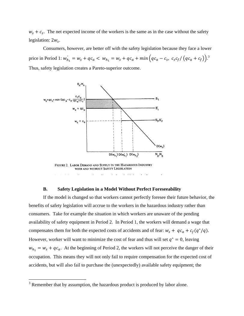
Consumers, however, are better off with the safety legislation because they face a lower

price in Period 1: .

3

Thus, safety legislation creates a Pareto-superior outcome.

B. Safety Legislation in a Model Without Perfect Foreseeability

If the model is changed so that workers cannot perfectly foresee their future behavior, the

benefits of safety legislation will accrue to the workers in the hazardous industry rather than

consumers. Take for example the situation in which workers are unaware of the pending

availability of safety equipment in Period 2. In Period 1, the workers will demand a wage that

compensates them for both the expected costs of accidents and of fear: .

However, worker will want to minimize the cost of fear and thus will set , leaving

. At the beginning of Period 2, the workers will not perceive the danger of their

occupation. This means they will not only fail to require compensation for the expected cost of

accidents, but will also fail to purchase the (unexpectedly) available safety equipment; the

3 Remember that by assumption, the hazardous product is produced by labor alone.

hazardous industry workers only demand . At this lower wage, more of the hazardous

product is demanded. In order to entice workers to move from the safe industry to the hazardous

industry, the industry must offer wages that compensate these new workers from the safe

industry (who correctly perceive the costs of accidents and thus purchase the safety equipment)

for purchasing safety equipment: . Not perceiving the hazards of their occupation,

the workers already in the hazardous industry will fail to use this extra wage to purchase safety

equipment. Thus their net wage is

.

If safety legislation is introduced which requires the hazardous industry workers to

purchase safety equipment in Period 2, these workers will incur the cost of the safety equipment,

but avoid the expected cost of accidents. Their net expected income thus becomes By

assumption , so and the workers in that entered the hazardous

industry in Period 1 are better off with the safety legislation.

C. Pre-Commitment Contracts

Next Akerlof and Dickens explore the possibility of workers entering into contracts in

Period 1 that bind them to purchase safety equipment in Period 2. Given the contract, workers

will have no incentive to choose a non-zero value for : they plan to purchase the safety

equipment in Period 2, so there is no reason to incur any unnecessary cost of fear in Period 1.

However, when Period 2 arrives, the workers will want to break their contracts. Since they have

chosen , they perceive no risk of accident and thus no need to purchase safety equipment.

Such workers will be willing to pay any amount up to to break the contract, as the safety

equipment as no value to them. Since the workers in Akerlof– Dickens model have perfect

foresight, they will know that entering into a contract in Period 1 is futile and won’t even attempt

to enter into them.

D. Bayesian Update Model

A Bayesian model can also be used to explain why workers in a hazardous industry might

choose not to adopt new safety equipment although it appears economically relevant to outsiders.

Unlike Akerlof–Dickens model, a Bayesian model does not necessarily suggest a need for safety

legislation. To construct the model, we will borrow most of the assumptions list above, except

those related to cognitive dissonance. In the Bayesian model, workers do not have the ability

choose to adopt whatever belief they choose about the safety level; in other words there is no .

We will also disregard the costs associated with “psychic fear.”

In this example, workers make two decisions in each over the two periods: where to work

and, if they are employed in the hazardous industry, whether to purchase safety equipment. In

addition, in Period 2, workers in the hazardous industry adjust their perception of risk based on

their personal experience (either of their own incident of accidents or of their observed incident

of accidents—here will assume it is based on their own incident of accidents). Let the new

perception of the risk of an accident be labeled qB. We can posit the following propositions:

1. The wage in the hazardous industry in Period 1 is ws + qca.

2. A worker in the hazardous industry in Period 2 chooses to buy safety equipment if:

qBca > cs.

3. The wage in the hazardous industry in Period 2 is ws + cs (assuming the workers

already in the industry are not able to increase output). If the workers in the

hazardous industry are able to increase output to meet demand, then the wage in

Periods 2 will be: wh1 = ws + min (cs, qBca).

Under this model it is possible that the workers in the hazardous industry will choose not to buy

safety equipment, this is especially true for workers who are less accident prone. In a situation

where the workers in the hazardous industry can increase output (so that there is competition

amongst the established workers) the Bayesian decision process will function to drive out

workers who are more accident prone.

V. Other Potential Applications

Incorporation of cognitive dissonance into economic models such as that described in this

paper may provide additional explanations for behavior that may otherwise appear irrational.

Akerlof and Dickens propose four additional areas in which a similar model of choice of beliefs

may be useful: (1) sources of innovation, (2) advertising, (3) Social Security, and (4) economic

theory of crime. For example, the authors note that economic understandings of the usefulness of

advertising may be improved by considering advertising as a source of external justification for

consumer beliefs that their purchases meet certain needs, essentially reinforcing their personal

beliefs about themselves. For the remainder of this presentation, I will focus on the potential for

this model to enhance understandings of the economic theory of crime.

Economists such as Tullock (1974) and Becker (1968) have previously applied price

theory to explain crime and punishment. These models suggest that, by increasing the cost of

crime, society can reduce the number of crimes committed. Thus, by increasing the probability

of detection or punishments imposed for crimes, the number of crimes committed can be

reduced. Recall that Becker further suggested that fines represent the smallest welfare loss to

society and may prove the best efficient punishment for crimes. These theories suggest that the

decision to commit crimes is based on a comparison of costs and benefits. However,

psychological experiments suggest that another factor is worthy of consideration: self-motivation

to obey the law. Motivated by cognitive dissonance theory, psychologists have found that a

threat of severe punishment can, once removed, increase the probability of a crime being

committed. In contrast, removal of a weaker punishment led to a smaller increase in probability

of a crime being committed. Akerlof and Dickens explain that these studies suggest that

individuals who decide not to commit crimes with small punishments are driven by an internal

belief in following the rules. In other words, they create an internal justification for their decision

to follow the rules. These individuals do not just compare costs and benefits of crime, but also

factor in their initial belief in following the rules. This initial belief favors following the rules

even when the threat of punishment is removed and explains the behavior found in the

psychological studies. In contrast, individuals deterred only from crime by the threat of severe

punishment are more likely to commit the crime once that threat is removed, since they did not

need to create such an internal justification. An important implication of this is that society’s

desire to inflict severe punishment for severe (costly) crimes should perhaps be tempered by the

fact that the threat of severe punishment reduces the self-motivation to obey the law, which

reduces crimes committed.