SuperWASP-N extrasolar planet candidates from fields - MNRAS

HAL Id hal-01182984httpshalarchives-ouvertesfrhal-01182984
Submitted on 5 Aug 2015
HAL is a multi-disciplinary open accessarchive for the deposit and dissemination of sci-entific research documents whether they are pub-lished or not The documents may come fromteaching and research institutions in France orabroad or from public or private research centers
Lrsquoarchive ouverte pluridisciplinaire HAL estdestineacutee au deacutepocirct et agrave la diffusion de documentsscientifiques de niveau recherche publieacutes ou noneacutemanant des eacutetablissements drsquoenseignement et derecherche franccedilais ou eacutetrangers des laboratoirespublics ou priveacutes
Astrophysics The Earth as an extrasolar transitingplanet II HARPS and UVES detection of water vapour
biogenic O 2 and O 3L Arnold D Ehrenreich A Vidal-Madjar X Dumusque C Nitschelm Richard
Querel P Hedelt J Berthier C Lovis C Moutou et al
To cite this versionL Arnold D Ehrenreich A Vidal-Madjar X Dumusque C Nitschelm et al AstrophysicsThe Earth as an extrasolar transiting planet II HARPS and UVES detection of water vapourbiogenic O 2 and O 3 Astronomy and Astrophysics - AampA EDP Sciences 2014httpwwwaandaorgarticlesaapdf201404aa23041-13pdf 1010510004-6361201323041hal-01182984
AampA 564 A58 (2014)DOI 1010510004-6361201323041ccopy ESO 2014
Astronomyamp
Astrophysics
The Earth as an extrasolar transiting planet
II HARPS and UVES detection of water vapour biogenic O2 and O3
L Arnold1 D Ehrenreich2 A Vidal-Madjar3 X Dumusque4 C Nitschelm5 R R Querel67 P Hedelt8 J Berthier9C Lovis2 C Moutou1011 R Ferlet3 and D Crooker12
1 Aix Marseille Universiteacute CNRS OHP (Observatoire de Haute Provence) Institut Pytheacuteas (UMS 3470)04870 Saint-Michel-lrsquoObservatoire Francee-mail LucArnoldosupytheasfr
2 Observatoire de Genegraveve Universiteacute de Genegraveve 51 ch des Maillettes 1290 Sauverny Switzerland3 Institut drsquoAstrophysique de Paris UMR7095 CNRS Universiteacute Pierre amp Marie Curie 98bis Boulevard Arago 75014 Paris France4 Harvard-Smithsonian Center for Astrophysics 60 Garden Street 02138 Cambridge USA5 Unidad de Astronomiacutea Facultad de Ciencias Baacutesicas Universidad de Antofagasta 601 Avenida Angamos Antofagasta Chile6 University of Chile Department of Electrical Engineering 2007 Tupper Avenue Santiago Chile7 National Institute of Water and Atmospheric Research (NIWA) 1010 Auchland Lauder New Zealand8 Deutsches Zentrum fuumlr Luft und Raumfahrt eV (DLR) Oberpfaffenhofen 82234 Wessling Germany9 Institut de Meacutecanique Ceacuteleste et de Calcul des Eacutepheacutemeacuterides Observatoire de Paris Avenue Denfert-Rochereau 75014 Paris
France10 Aix Marseille Universiteacute CNRS LAM (Laboratoire drsquoAstrophysique de Marseille) UMR 7326 13388 Marseille France11 CFHT Corporation 65-1238 Mamalahoa Hwy Kamuela Hawaii 96743 USA12 Astronomy Department Universidad de Chile Casilla 36-D Santiago Chile
Received 7 November 2013 Accepted 3 February 2014
ABSTRACT
Context The atmospheric composition of transiting exoplanets can be characterized during transit by spectroscopy Detections ofseveral chemical species have previously been reported in the atmosphere of gaseous giant exoplanets For the transit of an Earth twinmodels predict that biogenic oxygen (O2) and ozone (O3) atmospheric gases should be detectable as well as water vapour (H2O) amolecule linked to habitability as we know it on EarthAims The aim is to measure the Earth radius versus wavelength λ ndash or the atmosphere thickness h(λ) ndash at the highest spectralresolution available to fully characterize the signature of Earth seen as a transiting exoplanetMethods We present observations of the Moon eclipse of December 21 2010 Seen from the Moon the Earth eclipses the Sun andopens access to the Earth atmosphere transmission spectrum We used two different ESO spectrographs (HARPS and UVES) to takepenumbra and umbra high-resolution spectra from asymp3100 to 10 400 Aring A change of the quantity of water vapour above the telescopecompromised the quality of the UVES data We corrected for this effect in the data processing We analyzed the data by three differentmethods The first method is based on the analysis of pairs of penumbra spectra The second makes use of a single penumbra spectrumand the third of all penumbra and umbra spectraResults Profiles h(λ) are obtained with the three methods for both instruments The first method gives the best result in agreementwith a model The second method seems to be more sensitive to the Doppler shift of solar spectral lines with respect to the telluriclines The third method makes use of umbra spectra which bias the result by increasing the overall negative slope of h(λ) It can becorrected for this a posteriori from results with the first method The three methods clearly show the spectral signature of the Rayleighscattering in the Earth atmosphere and the bands of H2O O2 and O3 Sodium is detected Assuming no atmospheric perturbationswe show that the E-ELT is theoretically able to detect the O2 A-band in 8 h of integration for an Earth twin at 10 pcConclusions Biogenic O2 O3 and water vapour are detected in Earth observed as a transiting planet and in principle would bewithin reach of the E-ELT for an Earth twin at 10 pc
Key words Earth ndash Moon ndash atmospheric effects ndash planets and satellites atmospheres ndash planets and satellites terrestrial planets ndashastrobiology
1 IntroductionObserving planetary transits gives access to a set of propertiesof the star+planet system (eg Winn 2009) The relative size ofthe planet with respect to the star given by the depth of thetransit light-curve is one of the most straightforward systemobservables Spectrally resolved observations have shown forgaseous giant exoplanets that transit the brightest stars that thetransit depth varies with wavelength (the first to report this wereCharbonneau et al 2002 Vidal-Madjar et al 2003 2004) which
Based on observations made with ESO Telescopes at the La SillaParanal Observatory under programme ID 086C-0448
reveals the signature of the planetary atmosphere At certainwavelengths the atmosphere indeed absorbs the stellar light andbecomes opaque which makes the planet look larger in front ofthe star and produces a deeper transit The atmosphere of smallerterrestrial exoplanets close to or in the habitable zone (HZ)is in principle also accessible by this method (early works bySchneider 1992 1994 and more recent models by Ehrenreichet al 2006 2012 Kaltenegger amp Traub 2009 Garciacutea-Muntildeozet al 2012 Snellen et al 2013 Beacutetreacutemieux amp Kaltenegger2013) Recent simulations show that the next generation of in-struments in the infrared or visible domains that is the JamesWebb Space Telescope (JWST) and the European Extremely
Article published by EDP Sciences A58 page 1 of 18
AampA 564 A58 (2014)
Large Telescope (E-ELT) should be able to offer a first access tocharacterizing terrestrial planets in the HZ and detecting biosig-natures (here atmospheric O2 and O3) and molecules linked tohabitability (Rauer et al 2011 Hedelt et al 2013 Snellen et al2013 Rodler amp Loacutepez-Morales 2014)
In this context it is of prime interest to observe Earthas a transiting exoplanet Vidal-Madjar et al (2010) observedthe August 2008 partial lunar eclipse with the high-resolutionSOPHIE eacutechelle spectrograph at the 193 cm Haute-Provencetelescope (Perruchot et al 2008 Bouchy et al 2009) and showedthat the Earth atmosphere thickness versus wavelength can bederived from such observations Earth observed from the Moonduring a lunar eclipse indeed transits in front of the Sun andgives the possibility to study the Earth atmosphere as duringa transit These first observations also allowed one to iden-tify molecular species in the atmosphere that is water vapour(H2O) a molecule linked to Earth habitability biogenic oxygen(O2) and ozone (O3) Ozone and oxygen are considered as re-liable biosignatures for Earth-like planets (Owen 1980 Leacutegeret al 1993 Seager et al 2013) except for terrestrial planetsoutside the liquid-water habitable zone (Schindler amp Kasting2000) These species were also detected by Palleacute et al (2009)from umbra spectra taken during the same eclipse HoweverVidal-Madjar et al (2010) pointed out that the Palleacute et al spec-trum is not the transmission spectrum of Earth observed as adistant transiting planet The umbra signal indeed results fromphotons that are highly scattered and refracted by the deep atmo-sphere These photons strongly deviate from the star-planet di-rection and cannot be collected during the observation of a tran-sit From penumbra observations Vidal-Madjar et al (2010) ad-ditionally detected the thin high-altitude sodium Na I layer Thelarger diameter of Earth in the blue due to increasing Rayleighscattering at shorter wavelengths is also well visible althoughit is partially blended with residuals from spectrograph orderscorrection
In this paper we analyze new observations obtained duringthe lunar eclipse on Dec 21 2010 with the ESO spectrographsHARPS (from asymp3800 to 6900 Aring Mayor et al 2003) and UVES(from asymp3200 to 10 400 Aring Dekker et al 2000)
We present first the principle of the observation and differ-ent reduction methods the original Vidal-Madjar et al (2010)data reduction method (method 1) which makes use of a pair ofpenumbra spectra and a second method (method 2) which re-quires only one single penumbra spectrum to recover the atmo-sphere thickness profile (Sect 2) We also present a third alter-native method to derive the thickness profile which makes useof penumbra and umbra spectra This third approach is biasedby the refraction in the Earth atmosphere (Sect 3 method 3)but can be corrected a posteriori with the result of method 1An observation log and more details about the spectrographs aregiven in Sect 4 We give details on the data reduction in Sects 5and 6 for HARPS and UVES respectively The altitude profilesversus wavelength obtained with the three different methods aredetailed in Sect 7 as well as simulations of the E-ELT observinga transiting Earth twin at 10 pc
2 Principle of the observation (method 1 and 2)
The principle of Vidal-Madjar et al (2010) method is the follow-ing for an observer on the Moon in the deep penumbra the Sunappears above the Earth limb as a small crescent The light in thepenumbra is a mix of direct solar light that did not interact withEarth with light that passed through the (mostly upper) Earth
atmosphere The nature of this mixed light in the penumbra issimilar to what is observed during a transit of an exoplanet hereEarth in front of the Sun Nevertheless as seen from the MoonEarth is larger than the Sun and the Earth radius versus wave-length cannot be reconstructed from the transit depth et all wave-lengths as done with transiting exoplanets The method consistsof observing two different positions of the Sun above the Earthlimb (during ingress or egress) ndash that is of recording Moon spec-tra at two different depths in the penumbra (method 1) For thesetwo different positions on the Moon the solar crescent above theEarth limb as well as the arc of the Earth atmosphere intersect-ing the solar disk are different We have shown (Vidal-Madjaret al 2010 Eq (14) therein) that h the thickness profile of theatmosphere or the altitude under which the atmosphere can beconsidered as opaque can be written
h(λ) =
(EA(λ)EA(λ0)
times FA(λ0)FA(λ)
minus EB(λ)EB(λ0)
times FB(λ0)FB(λ)
)
divide(
LB
S Bminus LA
S A
) (1)
where E and F are the fluxes during the eclipse and outside thepenumbra (almost full-Moon just before or after the eclipse) re-spectively Subscripts A and B stand for the two different posi-tions in the penumbra The value λ0 is an arbitrary wavelengthfor which we define h(λ0) = 0 and the symbols S and L repre-sent geometrical parameters equal to the surface of the Sun cres-cent above the Earth limb and the length of the arc of the Earthatmosphere intersecting the solar disk for h(λ0) respectively (seeFig 4 in Vidal-Madjar et al 2010) Equation (1) shows that h(λ)can thus be written as a function of differences between the mea-sured fluxes divided by a factor of geometrical values The nu-merical values for S are recovered from the measured fluxestoo E(λ0) and F(λ0) following Eq (11) of Vidal-Madjar et al(2010)
E(λ0) = F(λ0) times SS (2)
where S is the surface of the solar disk At last once thesurfaces S are known the lengths L can be calculated quitesimply from geometrical considerations knowing the apparentdiameters of Earth and Sun so h(λ) can finally be calculated
Equation (1) above is obtained from the differences betweenEqs (12) and (13) in Vidal-Madjar et al (2010) each beingwritten for one position on the Moon These equations can berewritten for position A for example
h(λ) =
(1 minus EA(λ)
EA(λ0)times FA(λ0)
FA(λ)
)times S A
LAmiddot (3)
We note that h(λ) is fully calculable from Eq (3) above thuswith only one penumbra spectrum (method 2) Neverthelessbecause E and F are recorded at different times in the nightthe barycentric Earth radial velocity (BERV) leads to a dif-ferent Doppler shift between the solar and telluric lines in Eand F spectra Since we are interested in the signature of theEarth atmosphere all spectra are re-aligned on the telluric lineswhich slightly shifts the solar lines between E and F Moreoverthe solar lines integrated over the solar crescent seen from theMoon during the partial eclipse are also Doppler-shifted withrespect to the lines of the full (uneclipsed) solar disk The solarlines thus do not cancel out correctly in the ratio EA(λ)
EA(λ0) FA(λ)FA(λ0) and
the obtained h(λ) profile is noisier although the overall shape iscorrect With the difference in the left part of Eq (1) the solar
A58 page 2 of 18
L Arnold et al Earth as a transiting exoplanet observed during the 2010 lunar eclipse
lines cancel out much better and the h(λ) profile is cleaner Thisis discussed in more details in Sect 72
3 An alternative method that approximates h(λ)(method 3)
This section describes another method different from that ofVidal-Madjar et al (2010) to derive the thickness profile ofEarth atmosphere In a lunar eclipse the radius of Earth is givenby the radius of the umbra The umbra radius can be calcu-lated geometrically for a solid sphere that casts its shadow to theMoon but in practice the Earth atmosphere that scatters lightalong Earth limb lead to a blurred edge between umbra andpenumbra on the Moon surface The radiance profile across theumbra edge has been measured in the past by several observers(especially by Dubois from 1950 to 1980 Danjon 1925 Combazet al 1950 Reaves amp Walker 1952 Walker amp Reaves 1957) Theirradiance of the eclipsed Moon as well as the umbra edge havealso been modelized (Link 1969 Vollmer amp Gedzelman 2008Garciacutea-Muntildeoz amp Palleacute 2011) by an analysis of the light propa-gation from the Sun to the Moon through the Earth atmosphereThe observed magnitude versus position with respect to the um-bra center looks approximately like a hyperbolic function (orsigmoid) The observations mentioned above indicate that mag-nitude typically drops by about 8 mag from penumbra to umbrathe steepest region being typically 2 arcmin wide (Dubois ampPoumeyrol 1954) Unfortunately the spatial resolution of pub-lished radial photometry across the umbra edge is only about1 arcmin and not sufficient to reveal a dependance of the umbraradius with wavelength To fix the order of magnitude with anEarth umbra radius of asymp43 arcmin a variation of 10 km in theEarth radius (of 6371 km) translates into a change of the umbraradius of 4 arcsec
With ESOrsquos HARPS and UVES spectrographs we recordedspectra from deep penumbra to umbra over asymp7 arcmin withHARPS and asymp19 arcmin with UVES Because the telescopetracked neither the star nor the Moon but the Earth umbra pro-jected to the Moon we were able to integrate the signal at fixeddistances from the umbra edge while the Moon itself slowlyshifted in front of the spectrographs during the exposures Tocompare the flux in these spectra taken at different positions inthe umbra or in the penumbra we calculate their correspondingmagnitude minus25 log10(EF) relative to the full-Moon spectrarecorded before the eclipse Then we plot for each wavelengththe magnitudes versus their distance from the umbra center asDubois did But while Dubois observed at three or four dif-ferent wavelengths through broadband blue green yellow andred Wratten filters HARPS and UVES allow to do this now ata much higher spectral resolution The points follow the sameoverall shape as Duboisrsquo profiles (Fig 1) We fit a hyperbolicfunction through these points
ζ(r) = a0 + a1 tanh[a3(r minus a2)] (4)
where ζ is the model giving the magnitude in the radial direc-tion through the umbra edge r the distance to the umbra centerand ai the parameters defining the hyperbolic function The func-tion ζ(r) varies between a0 minus a1 and a0 + a1 We may arbitrarilydefine the abscissa a2 of the inflection point (at ordinate a0) ofthis function as a measurement of the umbra radius and thus ofthe Earth radius at the observing wavelength
Nevertheless Fig 1 shows that the inflection point corre-sponds to a zone about 3 mag (asymp15times) fainter than shallower
Fig 1 Measured magnitude across the umbra edge with HARPSat 5500 Aring Crosses and diamonds stand for A and B fiber respectivelyThe horizontal error bars are 2σ = 20 arcsec long and represent thetypical pointing error of the telescope Vertically the 2σ error bars arethe magnitude errors evaluated from the SN of the spectra at that wave-length and the evaluated error in the local Moon albedo The solid lineis the model from Eq (4) fitted through the data The vertical dottedline marks our definition of the umbra edge See Sect 73 for details
penumbra But in a real transit only the beams of light that in-teract with the top of the atmosphere and thus only weakly ab-sorbed leave a signature in the transit If a beam goes deeperto the atmosphere it is significantly dimmed and scattered andfinally absent from the transit signature of the planet Thereforethe informations from the 3 mag fainter light we obtain at theinflection point are not those we obtain during a real transit Theinflection point is thus not the best definition of the edge of theEarthrsquos umbra on the Moon at least in the context of our Earth-transit analysis It is more relevant to define a point slightly morein the brighter penumbra for the edge of Earthrsquos umbra as shownby the vertical dotted line in Fig 1 and to build up the Earthradius versus wavelength from this point instead of from theinflection point More details are given in Sect 73
We understand that this method makes use of informationthat is not available in an exoplanet transit indeed it uses in-formation from spectra of the umbra to build the function ζbut as mentioned in the introduction the photons from the um-bra result from highly angularly scattered or refracted beamswhich are not available in the observation of an exoplanet tran-sit Moreover the umbra photons especially the red ones havebeen refracted by the deepest Earth atmospheric layers and theEarth shadow is thus shrunk by refraction at these wavelengthsleading to a smaller Earth radius in the red In other words thegradient in the altitude profiles measured from blue to red wave-lengths will be steeper due to refraction But we show in Sect 73that the altitude profiles h(λ) obtained by this method can becalibrated (scaled) to the profiles obtained with method 1
4 Observing log
HARPS provides spectra with a spectral resolution of 115 000and covers the visible range (Table 1 Mayor et al 2003) UVESwas used in dichroic-1 and dichroic-2 modes (DIC1 and DIC2)
A58 page 3 of 18
AampA 564 A58 (2014)
Table 1 HARPS and UVES spectral ranges
Instrument Range (Aring) Gap (Aring)HARPS 3782ndash6912 5256ndash53375UVES DIC1 BLUE 3055ndash3885UVES DIC1 RED 4788ndash6806 5750ndash5821UVES DIC2 BLUE 3751ndash4999UVES DIC2 RED 6712ndash10 426 8544ndash8646
Notes Gaps without data are present in the final spectra due to smallgaps between detectors
Table 2 Series of n Moon reference spectra taken with HARPS beforethe eclipse
Start Exposure Airmasshminss UT (n times s)021826 4 times 30 215ndash212044120 5 times 45 170
Table 3 HARPS exposures and fiber positions in the penumbra (nega-tive values) and umbra (positive values) with respect to the umbra edgegiven by Guide-9
Start Exposure Fib A Fib Bhminss UT (s) (arcsec) (arcsec)064332 600 ndash66 41065728 450 ndash204 ndash98070635 300 ndash232 ndash125071307 900 36 141
Table 4 Series of three Moon reference spectra taken with UVES be-fore the eclipse
Start Exposure Mode and arm Mean airmasshminss UT (3 times s)020419 3 times 4 DIC2 RED 201020423 3 times 10 DIC2 BLUE 201021849 3 times 4 DIC1 RED 190021856 3 times 40 DIC1 BLUE 190050725 3 times 4 DIC2 RED 156050729 3 times 10 DIC2 BLUE 156051926 3 times 4 DIC1 RED 157051930 3 times 30 DIC1 BLUE 158
In each of these modes both BLUE and RED arms of the spec-trograph are used simultaneously and with standard settingstwo exposures (one in each mode) give a full [3100ndash10 400] Aringspectrum (Table 1 Dekker et al 2000) The slit width was setto 03 arcsec which gives a spectral resolution of asymp120 000
Tables 2 and 3 give information on the observations madefrom La Silla with HARPS The position with respect to theumbra edge was measured with Guide-91 Tables 4 and 5 givethe same information but for UVES at Paranal With UVES thetelescope was not positioned as expected on the Moon during theeclipse and the expected positions are indicated in parentheses inTable 5
As an example we show in Fig 2 the Sun seen from whereHARPS fiber-A was positioned on the Moon at 070635 UTat the beginning of the 300 s exposure (Table 3) The Sun issetting in the Pacific Ocean about 2000 km southeast of Japanat coordinates asymp156 E and asymp23 N The daytime cloud fraction
1 httpwwwprojectplutocom
Table 5 UVES exposures or series of n exposures and measured slitpositions in the penumbra (negative values) and umbra (positive values)with respect to the umbra edge given by Guide-9
Start Exposure Mode and arm Slit positionhminss UT (n times s) (arcsec)064519 2 times 40 DIC1 RED ndash210 (ndash90)064523 180 DIC1 BLUE ndash210 (ndash90)065107 3 times 20 DIC1 RED ndash233 (ndash180)065111 180 DIC1 BLUE ndash233 (ndash180)065801 600 DIC1 RED 577 (360)065805 600 DIC1 BLUE 577 (360)071508 2 times 60 DIC2 RED ndash220 (ndash90)071512 90 DIC2 BLUE ndash220 (ndash90)071935 2 times 25 DIC2 RED ndash229 (ndash180)071939 60 DIC2 BLUE ndash229 (ndash180)072230 20 DIC2 RED ndash147 (360)072234 20 DIC2 BLUE ndash147 (360)073510 600 DIC2 RED 936 (360)073514 600 DIC2 BLUE 936 (360)
Notes The expected slit positions are given in parentheses in the lastcolumn
Fig 2 Earth and Sun seen from the Moon deep penumbra whereHARPS fiber A was positioned at 070635 UT at the beginning ofthe 300 s exposure Image with Guide-9
for 2010 Dec 21 given by AquaMODIS2 for these coordinatesis geasymp07
5 HARPS data processing
The data processing makes use of so-called s1d reduced dataoutput files directly from the HARPS data reduction soft-ware (DRS) The HARPS instrumental response is calibratedwith a high signal-to-noise ratio (SN) G2V star spectrum
51 Correction for the Moon reflectivity
To accurately maintain a given position of the spectrograph withrespect to the umbra edge during the exposures we needed totrack the umbra not the Moon itself The Moon was thus mov-ing in front of the spectrograph pair of fibers at a speed of about055 arcsecs The shift of the Moon during a given exposurecontributed to smooth out any relative spectral reflectance dif-ferences between the lunar terrains that drifted in front of the
2 httpmodisgsfcnasagov
A58 page 4 of 18
L Arnold et al Earth as a transiting exoplanet observed during the 2010 lunar eclipse
Fig 3 Example of a path of the HARPS fibers across the reconstructedMoon image during the 300 s exposure in the penumbra The darkeningfrom the penumbra and umbra are not superimposed on the image heresince we are only interested in recovering the moon reflectivity The Aand B fibers remained at 232 and 125 arcsec from the umbra edge whilethe fibers path across the Moon was asymp164 arcsec long (length of the yel-low lines) The mean reflectivity is measured along the path taking intoaccount a 10 arcsec pointing error in both RA and Dec directions Theterrain reflectivity fluctuates by σ = 21 along the path for Fiber Aand σ = 15 for Fiber B in this highly contrasted lunar region Theerror on the mean reflectivity due to pointing uncertainty is estimatedto be about σ = 4 The figure shows that while Fiber A went throughthe dark region of Mare Nectaris Fiber B remained on a region mea-sured 39 brighter between Catharina and Cyrillus craters pointing outthe relevance of correcting the flux for lunar local reflectivity
spectrograph But different terrains with different albedos wereseen by each fiber during the different exposures To correct eachspectrum for the flux variations induced by these albedo varia-tions we measure the mean lunar reflectivity along the path ofthe slit across the Moon surface during the exposures a poste-riori The path is reconstructed from the date and telescope co-ordinates available in the metadata We build a picture of theMoon as seen during the eclipse from La Silla at a resolutionof 1 arcsecpixel the reconstructed scene is an orthographic pro-jection of a Clementine albedo map3 at 750 nm (Eliason et al1999) and takes into account the correct libration angles thecorrect phase angle (close of zero degree) and a Lambert-Lunarlimb-darkening law (Mc Ewen 1996) The mean lunar reflectiv-ity is then measured with Audela-204 along the path of eachfiber across the lunar surface as shown in Fig 3
52 Correction for the signature of the atmosphereabove the telescope
To correct our eclipse spectra for the signatures of the atmo-sphere above the telescope we need a reference transmissionspectra for the atmosphere T (λ) To derive T (λ) we proceedas in Vidal-Madjar et al (2010) by calculating the ratio oftwo full-Moon spectra F1 and F2 taken before the eclipse atdifferent airmass AM1 and AM2 lt AM1 The ratio can be scaledto AM = 1 following
T (λ) =
[FAM1
1 (λ)
FAM22 (λ)
](1(AM1minusAM2))
middot (5)
We calculate T (λ) with AM1 = 22 and AM2 = 17 (Table 2)Since we are interested only in the accurate measurement of the
3 httpwwwlpiusraedulunartoolsclementine4 httpwwwaudelaorg
Fig 4 La Silla atmosphere transmission function T (λ) for AM = 1 asevaluated from full-Moon spectra taken with HARPS just before theeclipse (Table 2) The spectrum is normalized at 6866 Aring To verifythis experimental T (λ) spectrum a transmission fit based on the modelof Hayes amp Latham (1975) for the Rayleigh and aerosol componentsnormalized at 6866 Aring is displayed (blue dashed line) We also add anozone transmission spectrum to the model (light-blue solid line) thatcorrectly fits the observed wide Chappuis band The best least-squaresfit for Rayleigh and ozone over La Silla that night is obtained for anairmass of AM = 077 for ozone and Rayleigh and an optical depthof 0181 at 5320 Aring for the aerosols between 4000 and 6866 Aring The fitfor ozone is made only where O2 and H2O absorption bands are absentThe O2 γ and B absorption bands are clearly seen around 6300 and6900 Aring respectively the other deep bands are due to H2O The smallgap in HARPS data is visible between 5300 and 5340 Aring (Table 1)
telluric lines in T (λ) the two spectra in Eq (5) are correctedfor the BERV to properly align the telluric lines of both spec-tra (the solar lines become slightly misaligned) Figure 4 showsthe obtained average reference transmission T (λ) that we nowuse in the following data analysis of HARPS data to re-evaluateall eclipse spectra as if they were collected from outside theatmosphere
6 UVES data processing
The UVES instrumental response is calibrated with the referencestar HD 80170 (K5 III-IV Teff = 4537 K log (g) = 21 Randichet al 1999)
61 Correction for the Moon reflectivity
To measure the mean lunar reflectivity along the path ofthe UVES slit across the Moon surface we build a picture ofthe Moon as seen during the eclipse from Paranal as we did forthe HARPS observations An example of the slit path is shownin Fig 5
62 Correction for the signature of the atmosphereabove the telescope
We can not proceed exactly as with the HARPS data be-cause full-Moon spectra show that the water-vapour lines were
A58 page 5 of 18
AampA 564 A58 (2014)
Fig 5 Example of a path of the UVES slit across the reconstructedMoon image during the 600 s exposure in the umbra The slit 10 arcseclong and perpendicular to the path remains at asymp936 arcsec from theumbra edge while the slit path over the Moon was asymp330 arcsec long(length of the yellow line) The mean reflectivity is measured along thepath taking into account a 10 arcsec pointing error in both RA and Decdirections The terrain reflectivity fluctuates by σ = 13 along the pathin this bright lunar region and the error on the mean reflectivity due topointing uncertainty is estimated to be about σ = 4
Fig 6 Part of the spectrum showing the ratio of a high airmass overa low airmass UVES full-Moon spectra The oxygen B and A bandsat 6900 and 7600 Aring respectively are in absorption as expected but thewater vapour bands at 7200 and 8200 Aring appear in emission showingthat the amount of water vapour along the line of sight was higher whenthe airmass was lower indicating that the amount of water vapour aboveParanal increased during the first part of the night before the eclipse Tocalculate this ratio the spectra are aligned by cross-correlation to matchthe radial velocity of the telluric lines so the solar lines do not properlycancel out in the ratio and appear with a wing in emission and the otherin absorption
stronger while the Moon was higher in the sky while it shouldhave been lower for the Moon at a smaller airmass Figure 6indeed shows that the amount of water vapour above the tele-scope increased during the first part of the night between thetwo sets of full-Moon observations We describe below how weconsequently corrected our UVES data
Table 6 Measured PWV before the eclipse and at the end the observa-tion and reduced PWV for airmass =1
hmin UT PWV Airmass PWV (mm) Note(mm) at zenith
0205 and 0218 643 201 320 10508 and 0521 800 156 514 20823 and 0832 595 104 571 3
Notes 1 full-Moon before penumbra ingress DIC2 and DIC1 obser-vations respectively 2 full-Moon before penumbra ingress DIC2 andDIC1 observations respectively First contact with penumbra occurredat about 0528 UTC 3 HD 80170 at the end of the eclipse observationDIC1 and DIC2 observations respectively
We estimate the precipitable water vapour (PWV) in ourspectra by using the spectral-fitting method described in Querelet al (2011) This method compares the measured spectrum witha reference spectrum while varying the reference water-vapourcontent The reference spectrum is generated using an atmo-spheric model configured with the local environmental parame-ters at the time of measurement (ambient temperature pressureelevation etc) A comparison is then made over several smallspectral intervals (asymp2ndash5 nm) where the only significant featuresare caused by absorption by water vapour A least-squares fit isperformed between the measured data and reference spectra for arange of PWV values The reference spectrum with the smallestfit residual represents the water-vapour content (or PWV) mostsimilar to that of the measured spectrum Since this absorptionis along the line-of-sight and assuming an isotropic distributionof water vapour above the telescope the absorption must thenbe corrected back to zenith by dividing the best-fit PWV by theairmass of the measurement
Table 6 indicates that three hours before the eclipsestarted the PWV measured on the full-Moon spectrum wasabout 64 mm for an airmass of 2 The PWV for air-mass =1 was therefore 32 mm Later in the night and justbefore the penumbra ingress we find that PWV increasedto 800 mm at airmass =156 indicating the increase of mois-ture above the telescope The reduced PWV for airmass =1 isthus 800156 = 51 mm before the eclipse started Immediatelyafter the eclipse observations we observed HD 80170 and mea-sured a reduced PWV of 571 mm We therefore assume thatduring the eclipse the PWV at zenith remains within the[51 57] mm range and we chose the mean value 54 mm asthe reference PWV at airmass =1 during the eclipse PWV val-ues of 5 mm are relatively high for Paranal and we understandthat assuming such a high water vapour content is isotropic andconstant above the telescope for three hours (the duration of ourobservations) may be a strong assumption Nevertheless it isthe best we can do and the whole process of data reduction lead-ing to h(λ) assumes the stability of the PWV above Paranal dur-ing the observations (this is obviously also true for the HARPSobservations at La Silla)
To correct our eclipse spectra for the signatures of the atmo-sphere above the telescope we need distinct reference transmis-sion spectra one for water and and one for oxygen In the follow-ing we describe how these reference spectra are obtained Thesereference transmission spectra do not need to include Rayleighand ozone signatures because they are already corrected for byUVES reduction pipeline
The UVES transmission water-vapour spectrum TH2O(λ) forairmass =1 (PWV = 54 mm) is obtained by the ratio of the
A58 page 6 of 18
L Arnold et al Earth as a transiting exoplanet observed during the 2010 lunar eclipse
full-Moon spectra F for which we know the value of PWV(Table 6)
TH2O(λ) =(F(PWV = 800)
F(PWV = 643)
)54(800minus643)
middot (6)
To derive a spectrum for pure water vapour (ie without thelines from other elements or molecules) TH2O(λ) is calculatedonly when water-vapour absorption is present (T le 99) inthe water-vapour synthetic spectrum computed to measure thePWV To avoid TH2O(λ) to become too noisy in the deepest ab-sorption bands of water vapour the spectrum is not calculatedwhen water-vapour transmission becomes T le 25
The transmission spectrum for O2 for airmass =1 is obtainedby taking into account the variation of airmass AM between thetwo F spectra (Table 6) as done by Vidal-Madjar et al (2010)
TO2(λ) =(F(AM = 201)
F(AM = 156)
)1(201minus156)
middot (7)
And as for TH2O TO2 is calculated only when O2 absorption ispresent (999 ge T ge 2) in a AM = 1 MODTRAN5 syntheticspectrum
Once TH2O and TO2 are known we can correct our spectrasimply by the division
s =S
(TH2O times TO2 )AM (8)
where s is the corrected spectrum and S is a full-Moon or eclipsespectrum acquired at airmass AM The final T (λ) spectrum forParanal is shown in Fig 7 The continuum shows neither theRayleigh nor the ozone signature in this spectrum (on the op-posite of what is obtained with HARPS Fig 4) because theUVES reduction pipeline automatically removed from all spec-tra tabulated values for the Rayleigh and ozone signatures at thecorresponding airmass of the observation Of course the addi-tional Rayleigh and ozone signatures present in the eclipse spec-tra and produced by the light path through the limb of the Earthatmosphere have not been removed by the UVES pipeline
To calculate TH2O and TO2 the full-Moon spectra are alignedwith a cross-correlation to match the radial velocity of thetelluric lines
7 Results and discussion
71 Results from Eq (1) (method1)
From the HARPS data we build five pairs of penumbra spectrasuitable for Eq (1) [98 204] [125 232] [66 125] [66 204]and [66 232] where the numbers in brackets are the positionsdescribed in Table 3 The possible pair [66 98] is not used itproduces a significantly noisier altitude profile probably becausethe positions in the penumbra are too close and the differencebetween the spectra is too small
The penumbra spectra are affected by the wavelength-dependent solar limb darkening LD(λ) (Hestroffer amp Magnan1998) Equation (1) makes use of geometrical parameters Sand L for two different solar crescents visible above Earth Thesolar LD(λ) makes the crescents fainter than the mean solarbrightness The size of the solar crescents estimated from thepenumbra spectra fluxes is thus underestimated if the penum-bra fluxes are not corrected for the solar LD To correct for
5 httpmodtran5com
Fig 7 Paranal atmosphere transmission function T (λ) for AM = 1 asevaluated from full-Moon spectra taken with UVES before the eclipsefollowing the reduction process described in Sect 62 The UVES re-duction pipeline automatically removes from all individual spectra tab-ulated values for the Rayleigh aerosol and ozone signatures at the cor-responding airmass of the observation These signatures therefore donot appear here as for HARPS (Fig 4) A weak residual curvature ofthe continuum (asymp5 maximum at 7800 Aring with no resemblance to aresidual signature of ozone or Rayleigh) was fitted with a second-orderfunction The spectrum shown here is normalized to this fit to have a flatcontinuum at 1 (horizontal line) The O2 γ A and B bands are clearlyseen (in red) the other bands are due to H2O (in blue)
this effect we first evaluate the size of the solar crescents (pa-rameters S and L) from the flux ratio (penumbrafull-Moon)at λ = 57988 Aring which allows us to evaluate an average LDthat affects each solar crescent following Hestroffer amp Magnan(1998) For these crescent sizes and the LD obtained at λ =57988 Aring a wavelength-dependant limb darkening LD(λ) is thenre-evaluated from the low spectral resolution model of Hestrofferamp Magnan (1998) It covers the spectral ranges [3033ndash3570]and [4160ndash10 990] Aring with a spectral resolution of a few tens(we do a linear interpolation between 3570 and 4160 Aring) Themodel is then used to calculate the LD-corrected penumbra spec-tra EA(λ)LD(λ) and EB(λ)LD(λ) from which new S and L areevaluated for λ0 with Eq (2) Equation (1) is then evaluatedagain to derive the final h(λ) profile
The mean altitude profile from the five pairs of fibers ob-tained from Eq (1) is shown in Fig 8 The profile is shiftedupward by asymp30 km to have an altitude of 238 km in the[4520ndash4540] Aring domain as predicted by Ehrenreich et al (2006)The profile shows the large bump due to ozone Chappuis bandcentered around 5900 Aring and peaking here at about 38 kmand the oxygen γ and B bands at 6300 and 6900 Aring respec-tively Water vapour also appears around 6500 Aring at an altitudeabove 25 km The increase of h(λ) in the blue due to Rayleighscattering is visible as a negative slope between 4000 and 5000 Aring(Ehrenreich et al 2006 Kaltenegger amp Traub 2009) The bluepart of the profile shows many residual solar absorption linesthat bias the binned profile towards lower altitudes Numeroussolar lines are visible for example Hβ at 4861 Aring and Hα at6563 Aring The Fig 9 is a zoom on the Na I doublet The asymp2 Aring-wide
A58 page 7 of 18
AampA 564 A58 (2014)
Fig 8 Altitude profile with HARPS as obtained from Eq (1)(method 1) A 10 Aring bin is superimposed in light-blue over the full-resolution profile The profile shows the large bump due to ozoneChappuis band around 6000 Aring the oxygen γ- and B-band at 6300 at6900 Aring respectively and also the water-vapour band around 6500 AringThe expected increased of h(λ) in the blue due to Rayleigh is visible asa negative slope between 4000 and 5000 Aring Oxygen and water-vapourabsorption spectra at arbitrary scale are shown
photospheric wings of the solar Na lines are still visible Thepresence of all these solar features indicates that the solar sig-nature is not properly removed from the h(λ) profile This couldresult from the EF ratios in Eq (1) The penumbra spectra Eindeed contain the spectrum from the solar crescent that isthe edge of the Sun where solar absorption lines are deeperthan in full-Moon spectra F which correspond to a full disk ofthe Sun illuminating the Moon We therefore tried to adjust apower p gt 1 on F to compensate for the solar residuals with ra-tios E(F p) in Eq (1) instead of EF But we found p to be veryclose to 1 and could not detect a significant difference betweenthe average depth of the absorption lines in E and F
Vidal-Madjar et al (2010) observe the same type of solarresiduals in the SOPHIE data (residual wings of the Na I dou-blet) and the explanation invoked is the Ring effect The depthof solar Fraunhofer lines in scattered light is lower than in di-rect sunlight This effect is known as the Ring effect (Graineramp Ring 1962) and is mainly induced by rotational Raman scat-tering (Vountas et al 1998) The line filling-in for forwardscattering (as experienced by the photons that interact withthe Earth atmosphere and are scattered towards the eclipsedMoon) is about 21 and 38 of the continuum for single andmultiple scattering respectively for the Ca II K line (Vountaset al 1998) Kattawar et al (1981) report a filling-in of 25at 63015 Aring for a Fe-I line Brinkmann (1968) calculates afilling-in of about 17 in the center to 19 in the wings fora hypothetical line at 4000 Aring underlining the continuous andsmooth effect across the line profile which is also measured byPallamraju et al (2000) Brinkmann (1968) reports observationsshowing a decrease of the filling-in with wavelength by a factorof 2 between 4383 and 6563 Aring and more recent measurements(Pallamraju et al 2000 Fig 3 therein) shows that the Ring effectdecreases approximately linearly by a factor of asymp3 from 4285
Fig 9 Zoom in the Na I doublet region of the altitude profile from Fig 8with HARPS and method 1 The asymp2 Aring-wide photospheric wings of theNa lines are still present showing that the solar signature is not properlyremoved from this h(λ) profile A residual solar line of Ni I is visibleat asymp58929 Aring (Wallace et al 2011)
to 6560 Aring for a given line strength (normalized depth to contin-uum times width)
Several methods exist to correct for the Ring effect (Wagneret al 2001) The simplest is that of Noxon et al (1979) whichconsists of subtracting a small constant close to 2 from thespectrum This was the solution applied in Vidal-Madjar et al(2010) where a constant is empirically adjusted to remove theresidual solar Na I lines (the constant was 4 and 06 of thecontinuum in the Na I region for the deepest and the shallowestpositions in the penumbra respectively) We also correct thisRing effect in our data
We observed that removing a Ring value xa from the shal-lowest spectrum in the penumbra and xb(gtxa) to the deepestspectrum gives almost the same result as removing xb minus xa tothe deepest only (all spectra were corrected from the instrumen-tal response so Noxonrsquos approach applies correctly) The Ringsignature is thus as expected stronger in the deeper spectrum(xb gt xa) where collected photons have been more scatteredin Earth atmosphere than photons collected in the shallowerpenumbra In our empirical correction for the Ring effect wetherefore only apply a correction on the spectrum in the deepestposition in the penumbra We consider empirical Ring correc-tions following i) Noxon et al (1979) ii) Noxon et al (1979)except in deep telluric bands (T lt 05) where the Ring effectis negligible because Raman-scattered photons are strongly ab-sorbed (Sioris amp Evans 2000) iii) a λminus2 power law to mimicthe chromatic dependance observed by Pallamraju et al (2000)or Brinkmann (1968) iv) a λminus2 power law subtracted except indeep telluric bands (T lt 05) and v) a subtraction of the recip-rocal of the spectrum (Johnston amp McKenzie 1989) that mimicsthe Ring spectrum Here again the obtained Ring spectrum isnot removed from deep telluric lines (T lt 05)
We observe that removing asymp1 of the continuum at 5880 Aringto the deepest spectrum of each pair reduces the solar residualsover the full altitude profile (Fig 10) and slightly reduces the
A58 page 8 of 18
L Arnold et al Earth as a transiting exoplanet observed during the 2010 lunar eclipse
Fig 10 Altitude profile with HARPS and method 1 without Ring cor-rection (upper panel) and different empirical Ring corrections Theamount of correction is 1 of the continuum at 5880 Aring i) Noxon et al(1979) ii) Noxon et al (1979) except in deep telluric bands (T lt 05)where the Ring effect is negligible because Raman-scattered photonsare strongly absorbed (Sioris amp Evans 2000) iii) a λminus2 power law tomimic the chromatic dependance observed by Pallamraju et al (2000)or Brinkmann (1968) iv) a λminus2 power law subtracted except in deeptelluric bands (T lt 05) and v) a subtraction of the reciprocal of thespectrum (Johnston amp McKenzie 1989) which mimics the Ring spec-trum Here again the obtained Ring spectrum is not removed from deeptelluric lines (T lt 05) The Na I doublet peaks at asymp5890 Aring for all typesof Ring corrections tested
Na wings (Fig 11) The correction also leads to the rise of theNa lines to altitude values of asymp80 km a value in agreement withthe literature (Plane 2003 Moussaoui et al 2010) Neverthelessthe width of the terrestrial Na I peaks are observed to be asymp04 AringThis is larger than the asymp02 Aring observed for the other tel-luric lines but might be induced by the presence of the strongNa I line in the solar spectrum The extraction process of h(λ) isthen more disturbed in the case of the Na I lines easily induc-ing a change in the width particularly because the solar linescannot be perfectly positioned in all spectra since these havebeen Doppler-shifted to have the telluric lines aligned An addi-tional effect is the limb-darkening effect that changes the shapeof the solar Na I lines emitted by different size crescent above theEarth limb This is also why the broad Na I stellar wings are notperfectly corrected in the presented extraction procedure whichonly includes a low spectral resolution limb-darkening modelFinally we also note that only the Na I lines are detected inFig 10 not the strong Mg I triplet at asymp5170 Aring nor Hα for
Fig 11 Same as Fig 10 but zoomed-in on the Na I doublet region ofthe altitude profile without Ring correction (upper panel) and differentempirical Ring corrections
example produce a peak in the altitude profile We thereforeconclude that the terrestrial Na layer is detected
Interestingly Garciacutea-Muntildeoz et al (2012) point out that thelunar eclipse of 16 August 2008 occurred only four days after themaximum of the Perseid meteor shower It is indeed known thatmeteor showers can temporarily increase the amount of sodiumin the atmosphere by a factor up of 10 (Plane 2003 Moussaouiet al 2010) This corroborates the detection of the sodium layerby Vidal-Madjar et al (2010) in August 2008 Nevertheless theGeminid meteor shower maximum occurs on December 13 Itis an active meteor shower with a particle density similar tothat of the Perseids6 that might have increased the sodium ab-sorption during the eclipse of 21 December 2010 Neverthelessour observations just show that the Na layer is indeed presentas during our first observations in August 2008 Since we haveonly one measurement it is unfortunately not possible to detectany change of the atmospheric Na I content either in 2008 orin 2010 and thus to confirm a link with any meteor shower
It can be seen from Fig 10 that the Ring correction is nothomogeneous across the full spectral range the Hα line remainsundercorrected while lines in the bluer part of the h(λ) pro-file are overcorrected We therefore adopt the simplest Noxon
6 See for example the IMO (International Meteor Organization)data at httpwwwimonetlivegeminids2012andhttpwwwimonetliveperseids2012
A58 page 9 of 18
AampA 564 A58 (2014)
Fig 12 Final altitude profile obtained with HARPS method 1 and with a Noxon correction for the Ring effect expect in the deep telluric lines(Sioris amp Evans 2000) A 10 Aring bin is superimposed in light-blue over the full-resolution profile 30 and 100 Aring bins are shown too shifted upwardsfor clarity The Na I peaks are visible near 5900 Aring Oxygen and water-vapour absorption spectra at arbitrary scale are shown The altitude profilehas been shifted to have an altitude of 238 km in the [4520ndash4540] Aring domain as predicted by Ehrenreich et al (2006) (dots and dashes in green ndashdashes to improve the visibility of the curve around 6000 Aring)
approach a subtraction of a constant except in deep telluriclines (T lt 05) The final result and the model from Ehrenreichet al (2006) are shown in Fig 12 The model is flatter than theobserved profile which peaks at about 35 km near 6000 Aring about8 km above the model This difference might be a refraction ef-fect that amplifies the observed profile as with method 3 al-though this effect is weaker here because we use only penum-bra spectra If the profile is calculated only with the two pairs[98 204] and [125 232] (Table 3) leaving out the spectrumfrom the deepest penumbra at only 66 arcsec from the umbrathe observed profile is indeed flatter (but noisier) it still peaksat 35 km higher that the altitude expected from the model butthe lowest altitude at 6900 Aring becomes asymp17 km instead of 12We note that our observations of the 2008 eclipse agrees bet-ter with the model (Vidal-Madjar et al 2010 Fig 9 therein) al-though SOPHIE fibers were between asymp100 and 250 arcsec fromthe umbra edge as for HARPS The additional bins in Fig 12show that the B-band is barely detectable in the 30 Aring bin whilethe broad O3 Chappuis band and Rayleigh slope in the blue re-main visible in the 100 Aring bin Figure 13 shows zooms in theNa I lines and the O2 γ and B band regions Oxygen shows upvery clearly with peaks reaching h = 35ndash40 km Some water-vapour peaks are visible but weak which is not surprising be-cause of the high altitude at which they are detected and alsobecause of the lower strength of the water-vapour absorption inthe HARPS wavelength range compared with λ gt 7000 Aring Wedetect neither Li (6708 Aring) nor Ca II (Hunten 1967 Plane 2003)
With UVES the coordinates of the telescope indicate that thetelescope unfortunately did not move in the penumbra betweenthe exposures in order to record spectra at 90 and 180 arcsecfrom the umbra edge as expected but instead stayed asymp200 arcsecfrom the umbra (Table 5) The different recorded spectra arevery similar and the result from Eq (1) is noisy especially inthe blue Residuals from spectral orders are also visible above7000 Aring There is nevertheless a spectrum taken in UVES DIC2
configuration while the telescope was thought to be in the um-bra but was too close to the Moon edge and left the moon about20 s after the exposure started The exposure was then stoppedbut the telescope coordinates indicate that the telescope was infact in the penumbra The exposure time for that unexpected ex-posure is only about 21 and 38 of what was required for theBLUE and RED exposures respectively The altitude profile ob-tained with UVES is shown in Fig 14 The overall shape agreeswith the model of Ehrenreich et al (2006) but the altitude ob-served in the UV is far higher than that of the model Moreoverwe had to shift the DIC1 BLUE profile by ndash110 km to connectit to the DIC2 BLUE profile The DIC2 RED profile has also tobe shifted by 35 km to be connected to the altitude obtained forthe DIC1 RED profile The oxygen bands are barely visible andthe water-vapour bands appears in absorption We did not con-sider any Ring correction for this noisy profile Note also thatthe model of Ehrenreich et al (2006) shown in the figures of thispaper does not include water vapour
72 Results from Eq (3) (method 2)
The HARPS spectra are now used with Eq (3) to calculate hfrom only one penumbra spectrum The eclipse spectra are cor-rected for limb-darkening and Ring effect as for method 1 Whenthe profile is calculated with the spectra in Eq (3) aligned onthe telluric lines the solar lines become consequently slightlymisaligned which generates noise in the profile (Fig 15 upperpanel) We therefore build a composite profile where all linesndash telluric and solar ndash are aligned The composite uses two dif-ferent profiles one aligned on the telluric lines and a secondaligned on the solar line In the first profile every misalignedsolar line is recognized with the help of a synthetic G2 spec-trum and replaced by its aligned residual taken from the secondprofile Some solar lines are missing in the G2 spectrum in themost crowded telluric bands therefore some residual noise due
A58 page 10 of 18
L Arnold et al Earth as a transiting exoplanet observed during the 2010 lunar eclipse
Fig 13 Zooms on the HARPS final altitude profile from method 1(Fig 12) with a Noxon correction for the Ring effect except in the deeptelluric lines (Sioris amp Evans 2000) Oxygen and water vapour absorp-tion spectra at arbitrary scale are shown Oxygen shows up very clearlyWater vapour is barely visible around 6500 Aring above 25 km and weaklines are visible in the higher Na I D1 D2 region Note that our Noxoncorrection does not completely remove the wings of the Na I solar linesThe wings disappear with a stronger correction but the two Na I peaksthen reach an altitude well above 100 km which is not realistic
to uncorrected solar lines is still present in the composite in-side these telluric bands The procedure still slightly cleans the hprofile (Fig 15 lower panel) The overall shape of the profileis similar to the profile obtained with Eq (1) shown in Fig 12Ozone appears about 6 km above the model When zooming-in (Fig 16) only the oxygen B and γ bands are correctly de-tected with peaks reaching h = 35ndash40 km Water-vapour bandsat 6500 and 5890 Aring are not visible nor the atmospheric Na I D-lines which are maybe hidden in the strong solar residual linesNote that the profile shown here is for the deeper position in thepenumbra The other positions lead to a noisier result althoughthe overall shape is correct
Equation (3) is also applied on UVES spectra to calculate hAs for HARPS we compute a composite profile The compositeis the profile obtained with the spectra aligned on the solar linesin which the oxygen and water-vapour lines are replaced by theoxygen and water-vapour lines picked up in the profile obtainedwith the spectra aligned on the telluric lines This procedurecleans the profile (Fig 17 lower panel) although compromisingthe detection of atmospheric species different from oxygen andwater This may explain at least partially why the Na I D-linesdo not appear clearly The oxygen γ B and A bands are visibleup to asymp80 km (zooms in Fig 18) but water-vapour bands arenot detected We subtract a Ring effect from the UVES eclipse
Fig 14 Final altitude profile obtained with UVES and method 1 NoRing correction is applied A 10 Aring bin is superimposed in light-blueon the full-resolution profile Reference oxygen and water-vapour ab-sorption spectra obtained with UVES are shown at arbitrary scale Thealtitude profile has been shifted to have an altitude of 238 km in the[4520ndash4540] Aring domain as predicted by Ehrenreich et al (2006) (greendashed line no water vapour in the model)
Fig 15 Altitude profile with HARPS and Eq (3) (method 2) Only thespectrum of the deepest penumbra taken at 66 arcsec from the um-bra is used here (Table 3) Shallower penumbra spectra give similar butnoisier profiles A 10 Aring bin is superimposed in light-blue on the full-resolution profiles The upper panel shows the profile obtained withthe HARPS spectra aligned on the telluric lines Solar lines are conse-quently slightly misaligned and generate noise in the profile The lowerpanel shows a composite profile showing the profile calculated with thespectra aligned on the telluric lines expect when a solar line is presentwhere the profile from spectra aligned on the solar lines is used Oxygenand water-vapour absorption spectra at arbitrary scale are shown Thegreen dashed line is the model of Ehrenreich et al (2006)
A58 page 11 of 18
AampA 564 A58 (2014)
Fig 16 Zooms on the HARPS altitude profile from method 2 shown inFig 15 Oxygen and water-vapour absorption spectra at arbitrary scaleare shown to facilitate the identification of the spectral lines Oxygenis correctly detected while water vapour is not detected AtmosphericNa I D-lines are not detected either maybe they are hidden by the strongsolar residual lines
spectra of 05 of the continuum at 5880 Aring When we subtracta Ring effect of 1 as we did for HARPS the profile does notchange except from the oxygen A and B bands which peak at150 km
Qualitatively speaking the overall shape of the profile from3000 to 7000 Aring is in acceptable agreement with the model withthe ozone Chappuis bump at 6000 Aring and a Rayleigh increaseof h in the blue and near UV The DIC2 BLUE altitude is setto h = 238 km in the [4520ndash4540] Aring domain as predicted byEhrenreich et al (2006) The other parts of the profile need to beshifted by about plusmn6 km to be properly continuously connectedto the DIC2 BLUE profile
73 Results from the umbra edge radiance profile(method 3)
With method 3 we make use of all available umbra and penum-bra spectra The penumbra spectra are corrected from the limb-darkening in the same way as for method 1 and 2 For each sam-pled wavelength in the HARPS spectra we fit a sigmoid curve(Eq (4)) through the eight available measured points (positionmagnitude) in the umbra and deep penumbra region (Table 3)An example of the obtained fit is shown in Fig 1 We now needto define the radius of the umbra edge re from which we build
Fig 17 Altitude profile with UVES and method 2 A 10 Aring bin is su-perimposed in light-blue on the full-resolution profile The upper panelshows the profile obtained with the UVES spectra aligned on the telluriclines with solar lines consequently slightly misaligned and thus gener-ating noise in h The lower panel shows a composite profile showingthe profile aligned on the solar lines when no telluric line is presentand the profile aligned on the telluric lines when a telluric line ispresent Oxygen and water-vapour absorption spectra at arbitrary scaleare shown to facilitate the identification of the spectral lines The modelof Ehrenreich et al (2006) is shown in green
the Earth atmosphere thickness h(λ) simply given by
h(λ) = re(λ) times roplusru+ cte (9)
where re is expressed in arcmin ru = 427 arcmin is the umbraradius from the ephemeris and roplus = 6371 km is the Earth radiusThe constant cte is set to give h = 238 km at [4520ndash4540] Aring
As explained in Sect 3 the inflection point abscissa a2 of thefit is not the best estimate of re (in our context of Earth transitanalysis at least) To explore the impact of re on h(λ) we write resuch that
ζ(re) = a0 + c times a1 (10)
For the inflection point the coefficient c in front of half-amplitude a1 of the tanh function is c = 0 and ζ(a2) = a0Positive values of c lead to positions on the penumbra side ofthe inflection point Figure 19 shows a set of altitude profilesbuilt for different positions across the umbra edge with minus06 ltc lt 09 as shown in Fig 20 The profiles versus c change sub-stantially for c = minus06 the profile is built from data on theumbra side of the inflection point and the bump from the ozoneChappuis band is almost invisible The mean negative slope ofthe profile also underlines the effect of refraction that shrinksthe Earth umbra at redder wavelengths This effect decreaseswhen c increases to positive values with the profiles built fromdata on the penumbra side of the inflection point The broadChappuis band is detected We finally define the umbra radiussuch as ζ(re) = a0 + 06 times a1 (c = 06) For this value thenoise in the altitude profile is close to minimum and the biasfrom shallow umbra (that is the mean negative slope of h(λ))is reduced With this definition Fig 20 puts the umbra edge at
A58 page 12 of 18
L Arnold et al Earth as a transiting exoplanet observed during the 2010 lunar eclipse
Fig 18 Zooms on the oxygen A and B-band regions of the UVES profilshown in Fig 17 (method 2) An oxygen absorption spectrum at arbi-trary scale is shown
about 1 arcmin in the penumbra side with respect to the inflec-tion point and about one magnitude fainter than the penumbraat 4 arcmin from the inflection point This choice is consistentwith our reasoning developed Sect 3
The result with HARPS and method 3 is shown in Figs 21and 22 Wide and narrow features of the Earth atmosphereare visible (Rayleigh ozone Chappuis band oxygen γ andB-bands) Water vapour is not detected suggesting it is notpresent above 12 km Compared with the profile obtained withmethod 1 (Fig 12) the profile with method 3 shows a strongernegative slope from blue to red leading to an altitude rangeabout asymp33 times larger than with method 1 We attribute thiseffect to the fact that method 3 makes use of umbra spectra Thelight in the umbra is reddened by Rayleigh scattering in the deepEarth atmospheric layers and refracted towards the umbra centerTherefore the umbra edge in red light is more refracted towardsthe umbra center than at blue wavelengths The umbra radius(Earth radius on the Moon) is thus smaller in the red than in the
Fig 19 Altitude profiles obtained with HARPS and method 3 for differ-ent positions across the umbra edge given by parameter c in Eq (10)and shown in Fig 20 The vertical axis is the measured altitude setto 238 km at at [4520ndash4540] Aring for the profile calculated for c = 0Other profiles are shifted vertically for clarity by steps of 40 km Theprofiles in this figure are not built at HARPS native resolution but at asmaller asymp06 Aringpixel resolution The light-blue lines are 10 Aring bins
Fig 20 Positions across the umbra edge used to build the altitudeprofiles shown in Fig 19 The positions are defined by parameter c(Eq (10)) and ranging from c = minus06 to 09 The definition for theumbra edge is taken for c = 06 (vertical solid line) at asymp1 arcmin inthe penumbra side with respect to the inflection point here fixed at ab-scissa =0 The umbra edge is only about one magnitude fainter than thepenumbra at 4 arcmin from the inflection point
A58 page 13 of 18
AampA 564 A58 (2014)
Fig 21 Altitude profile obtained with HARPS and method 3 The left vertical axis is the measured altitude set to 238 km at at [4520ndash4540] AringThe right vertical axis is the corrected altitude if one considers the lowest region of h close to altitude 12 km as in Fig 12 and again h = 238 kmat [4520ndash4540] Aring The horizontal dotted line represents the altitude 238 kmThe light-blue line is a 10 Aring bin superimposed on the full-resolutionprofile Oxygen and water-vapour absorption spectra at arbitrary scale are shown
Fig 22 Zooms on the HARPS altitude profile from method 3 shown inFig 21 The left vertical axis is the measured altitude set to 238 km at[4520ndash4540] Aring The right vertical axis is the corrected altitude if oneconsiders the lowest region of h close to altitude 12 km as in Fig 12and again h = 238 km at [4520ndash4540] Aring Oxygen and water-vapourabsorption spectra at arbitrary scale are shown Water vapour is not de-tected above 16 km suggesting that the amount of water vapour is toolow to absorb enough to be visible at this altitude The sodium layerNa I is not detected
Fig 23 Measured magnitude across the umbra edge with UVESat 10 000 Aring The horizontal error bars are 20 arcsec long and repre-sent the typical pointing error of the telescope Vertically the 2σ errorbars are the magnitude errors given by the UVES pipeline and the eval-uated error in the local Moon albedo The solid line is the model fromEq (4) fitted through the data with parameter a3 set to the mean valueof a3 found for the HARPS data The vertical dotted line marks the edgeof the umbra following our definition
blue due to refraction and Rayleigh scattering This effect am-plifies the measured altitude range across the full visible spec-trum To correct for this effect the right vertical axis of Fig 21is calibrated with the method 1 result by setting the altitude fortwo different points that is the lowest region of h at altitude12 km and h = 238 km at [4520ndash4540] Aring
A58 page 14 of 18
L Arnold et al Earth as a transiting exoplanet observed during the 2010 lunar eclipse
Fig 24 Altitude profile obtained with UVES and method 3 The left vertical axis is the measured altitude set to 238 km at [4520ndash4540] Aring Theright vertical axis is the corrected altitude if one considers the lowest region of h close to altitude 0 km and again h = 238 km at [4520ndash4540] AringThe horizontal dotted line represents the altitude 238 km A 10 Aring bin is superimposed in light-blue on the full-resolution profile and a 100 Aring binin red is also shown shifted upwards for clarity The profile for λ le asymp4300 Aring is not shown because the very weak umbra signal induces noise inthe altitude profile which becomes noisy and h unexpectedly decreases Oxygen and water-vapour absorption spectra at arbitrary scale are shown
We process the UVES data in the same way Neverthelesssince we have less observations points with UVES than withHARPS it is not possible to keep four free parameters forthe fitting function the sigmoid ζ We have to fix the a3 pa-rameter to the mean value obtained with HARPS The param-eter a3 describes the steepness of the fit near the inflectionpoint and is quite stable for HARPS at visible wavelengths inthe [6500ndash6900] Aring range its average value is a3 = 988 times 10minus3
with an RMS of σ = 22times10minus4 We fix a3 to that mean value forUVES An example of the fit through the UVES observationsat 10 000 Aring is shown in Fig 23 Figure 24 shows the altitudeprofile obtained with UVES showing the same features as forHARPS with clear oxygen A and B bands and water-vapourbands up to 10 000 Aring As with the HARPS profile (Fig 21) theprofile obtained with UVES displays a strong global negativeslope Here the profile is asymp45 times larger than with method 1The right axis in Fig 24 is calibrated considering that the lowestregion of h is close to altitude 0 km and again that h = 238 kmat [4520ndash4540] Aring The factor of 45 is larger than with HARPS(asymp33) maybe because the slit positions with UVES are deeperin the umbra than with HARPS (see Tables 5 and 3)
In the blue (λ le asymp4300 Aring) the signal in the umbra spectrais weak and the altitude profile becomes noisy and unexpectedlydecreases (this part of the profile is not shown in Fig 24) Theweak signal in the deepest lines of oxygen A-band and watervapour (asymp9300ndash9500 Aring) in the umbra spectra is also responsi-ble for spikes above 100 km at these wavelengths To cancel outmost of these spikes we set a flux threshold for the umbra spec-tra of 1 of the continuum below which the algorithm does notevaluate h At last to have h = 238 km at [4520ndash4540] Aring wesubtract 37 km from the DIC2 BLUE profile To have all parts ofthe profile connected in Fig 24 we shift the DIC1 RED profileby ndash23 km and the DIC2 RED profile by +25 km
The Figs 25 and 26 show zooms in the UVES full profileshown in Fig 24 In Fig 25 the three oxygen bands are clearly
detected Note that the core of the oxygen line for the A-bandcould not be calculated because the signal in the line core is tooweak The sodium layer is not detected and no water vapourappears above 19 km near the sodium lines At λ gt 7000 Aringin Fig 26 water vapour appears very well even at an altitudehigher than 20 km because the water-vapour absorption bandsbecome stronger in these longer wavelengths Water vapour in-deed presents a vertical distribution in the Earth atmosphere andis thus also present at higher altitudes but with lower volumedensities The altitude at which it is detected (where an opticalthickness of about 1 is reached for a grazing line of sight) is ofcourse higher in the stronger bands
It is worth noting that the residuals of the Na I lines are verysimilar apart from the noise for HARPS and UVES (Figs 22and 25 respectively) This is expected because HARPS andUVES observed roughly the same solar crescents and thus expe-rienced the same Doppler shift of the solar lines of the crescentsthat induced these residuals in the altitude profile Note also thatno correction of the Ring effect is implemented in method 3 ei-ther for HARPS or UVES All spectra are indeed used here allat different depths in the penumbra and umbra A simple empiri-cal approach cannot reasonably be considered A physical modelof the Ring effect is much needed taking into account the pathlength through the Earth atmosphere for the different positionsobserved in the umbra and penumbra
74 Possibilities with a future giant telescope
We analyze how our results can be extrapolated to what a futureground-based giant telescope might be able to detect in the visi-ble transmission spectrum of an Earth-like exoplanet observedin transit We use a full model of the future E-ELT a 39 mtelescope The focal instrument has the same throughput pixelsampling and detector characteristics as the EPICS instrumentsThe model takes into account the photon noise from the starthe thermal and readout detector noises the zodiacal noise and
A58 page 15 of 18
AampA 564 A58 (2014)
Table 7 Transit of an Earth twin at 10 pc observed for 8 h by the E-ELTat low spectral resolution and assuming no atmospheric perturbations
Filter λ range h SN δ h plusmn 1-σ(Aring) (km) error (km)
O3 + Rayl 1 5000ndash5500 199 113 172 plusmn 30O3 + Rayl 2 5500ndash6100 192 123 165 plusmn 29O3 + Rayl 3 6300ndash6800 150 86 123 plusmn 29O2-B 6865ndash6905 176 25 148 plusmn 64Rayl 4 7360ndash7560 89 31 62 plusmn 32O2-A 7590ndash7650 232 37 205 plusmn 59Rayl 5 7750ndash8100 72 33 45 plusmn 29Rayl 6 8450ndash8800 53 23 26 plusmn 28Water vapour 9300ndash9600 87 31 60 plusmn 32Window 10 100ndash10 400 27 10 0 plusmn 26
Notes The SN is calculated through ten different filters The last fil-ter ldquoWindowrdquo is for the atmospheric window The filter widths rangefrom 40 Aring for the O2 B to 600 Aring for one of the filter sampling theChappuis band The values of h are taken from the 10 Aring bin of theUVES profile (Fig 24) The value δh is the altitude difference to theatmospheric window measured by the E-ELT
the absorption of the local atmosphere above the telescope (seeHedelt et al 2013 for a detailed description of the model)
We define a set of ten filters i) to sample the Chappuis bandand the Rayleigh continuum and ii) to isolate the most interest-ing narrow features in the profile shown in Fig 24 that is theoxygen A and B bands and the water vapour around 9500 AringThe low spectral resolution 10 Aring bin in this figure shows thatthe oxygen A-band peaks about 20 km above the lowest altitudearound 10 200 Aring The Earth radius is thus 03 larger andthe transit 06 deeper through a filter that isolates the oxy-gen A-band The Earth transit depth is 83 times 10minus5 and the tran-sit variation at that spectral resolution for the O2 band repre-sents 75 times 10minus7 of the stellar flux
According to Porto de Mello et al (2006) there are 33 solar-type stars within 10 pc 13 of which are reasonably similar tothe Sun in terms mass age metallicity and evolutionary sta-tus Considering that the transit probability of an Earth twin infront of its star is about 1 we understand that the probabil-ity of detection is low even if all stars have a planet in theirhabitable zone The Darwin All Sky Star Catalogue (Kalteneggeret al 2010) lists 878 single FGK stars within 30 pc a num-ber fully consistent with the 33 solar-type stars numbered byPorto de Mello et al (2006) for a 27 times smaller volumeNevertheless although the probability of transit detection sig-nificantly increases with 878 targets the flux for a star at 30 pcwill be 9 times fainter than at 10 pc meaning that 9 times moretransits will be necessary to reach the same SN as for a targetat 10 pc
We consider an earth at 10 pc transiting a G2V star ob-served during a full night of 8 h (an Earth-like 13 h single transitbeing longer than the night) The simulation assumes that theatmosphere above the telescope is perfectly stable The simula-tion results are given in Table 7 and shown in Fig 27 The resultshows that transit photometry through the defined filters allowsin principle the detection of the O2 A-band with a detection levelof asymp23 σ The oxygen B and water-vapour bands will be moredifficult to detect and will require more than one transit to reacha detection level gt2σ This is also true for the ozone Chappuisband which is blended with the Rayleigh scattering
It is encouraging to see that the E-ELT will beat the photonnoise in only one single transit to identify oxygen in the visible
Fig 25 Zooms on the UVES altitude profile from method 3 shown inFig 24 The UVES oxygen spectrum at arbitrary scale is shown Thethree oxygen bands are clearly detected Note that we were unable tocalculate the core of the oxygen line for the A-band because the signalin the line core is too weak The sodium layer is not detected Water-vapour absorption is too weak in the Na I region to appear above 19 km
range on a terrestrial planet transiting a solar-type star at 10 pcBut it will be extremely difficult at least at low spectral resolu-tion to detect the 75times10minus7 flux variation in the O2 band throughthe slightly fluctuating atmosphere above the telescope
We considered broadband and narrow-band photometrywith a spectral resolution of up to asymp170 But it is worth notingthat at a much higher spectral resolution (of the order of asymp105)the telluric lines become distinct from those of an exoplanet assoon as its radial velocity is sufficiently different from the BERVUnder these conditions ground-based detection at high spectralresolution of O2 or H2O in an exoplanet atmosphere becomeseasier especially by cross-correlating the transit spectrum andan O2 or H2O spectrum respectively (Vidal-Madjar et al 2010Snellen et al 2013 Rodler amp Loacutepez-Morales 2014)
8 Summary and conclusion
We have described the analysis of the observations of a lunareclipse used as a proxy to observe Earth in transit The resultsfully confirm those obtained with SOPHIE and the observationof the August 2008 eclipse (Vidal-Madjar et al 2010) and ex-tend the observed h(λ) profile towards the near infrared thanksto the UVES data They agree well with the models (Ehrenreichet al 2006 Kaltenegger amp Traub 2009 Snellen et al 2013Beacutetreacutemieux amp Kaltenegger 2013) The Rayleigh increase in theblue is visible Biogenic oxygen and ozone are also well visible
A58 page 16 of 18
L Arnold et al Earth as a transiting exoplanet observed during the 2010 lunar eclipse
Fig 26 Zooms on the UVES altitude profile from method 3 shown inFig 24 The UVES water-vapour absorption spectrum at arbitrary scaleis shown Water vapour is very well detected even at an altitude above20 km at λ gt 8000 Aring where the water-vapour absorption is the strongestin the UVES wavelength domain
in the atmosphere altitude profiles and are therefore relevant de-tectable biosignatures to look for during transits of Earth-likeexoplanets in the [4000ndash10 500] Aring range The oxygen A andB bands show up clearly with HARPS or UVES
Water vapour is well detected at λ gt 8000 Aring with UVES be-cause water-vapour absorption is stronger at these wavelengthsTherefore even low densities of water vapour at these altitudesare detected Water vapour is seen at an altitude of up to 20 kmaround 9500 Aring Moreover Rayleigh scattering and ozone ab-sorption are essentially absent above 8000 Aring therefore we arealso able to probe deeper layers in the Earth atmosphere wherelow-altitude water vapour is also present at higher densities InHARPS data at λ lt 7000 Aring water vapour appears above 25 kmwith method 1 but remains below 25 km with method 2 and be-low 12 km with method 3 because water-vapour absorption isweaker in the visible range
The results from UVES are nevertheless less reliable thanthose of HARPS because the PWV was not stable during the be-ginning of the night when the calibration spectra were recordedon the full-Moon before the eclipse which compromised thequality of the eclipse observation Although we were able to re-cover the water-vapour content in the calibration spectra a pos-teriori the results for the detection of water vapour in the al-titude profiles with UVES are not coherent between method 12 and 3 This underlines the difficulties of these observationswhich were made through the local atmosphere above the tele-scope while our goal was to measure atmospheric features at a
Fig 27 Simulated observations with the E-ELT of an Earth twin at10 pc transiting a G2V star at low spectral resolution and assumingno atmospheric perturbations (Table 7) The simulated observations areshown in red The horizontal bars represent the filter bandwidth and thevertical error bars are the plusmn1σ estimated error from the model The solidline is the 10 Aring bin UVES profile (method 3)
planetary scale Lunar eclipse observations done from space ei-ther at low or high spectral resolution would not suffer from thetelluric pollution with the additional benefit of an access to UVand the prominent Hartley band of ozone
Another bias in the recovering of the Earth atmosphere pro-file from a lunar eclipse is the effect of refraction in method 3that makes use of refracted light from the umbra We have shownthat this effect can be partially corrected with the results frommethod 1 but the profiles ndash either from HARPS or UVES ndash stillshow a residual negative slope with respect to the profile frommethod 1 or 2
Finally these results provide input for the preparation of fu-ture observations with the next generation of giant telescopesWe showed that the E-ELT observing in the visible rangeat low spectral resolution and in the absence of atmosphericperturbations is in principle able to detect the O2 A-band in theatmosphere of a transiting Earth twin It will be extremely chal-lenging in practice through the atmosphere If we overcome thisdifficulty especially with high spectral resolution spectroscopythe O2 signature may then be increasing from year to year (fromtransit to transit) as will the enthusiasm of the observers
Acknowledgements We thank Gaspare Lo Curto (HARPS) and Claudio Meloand Lorenzo Monaco (UVES) for their help in the preparation of these relativelyunusual observations as well as the teams who operated the telescopes that nightWe also thank I Snellen and the referee W A Traub for their constructivecomments on the manuscript R R Querel acknowledges funding from Conicytthrough Fondecyt grant 3120150
ReferencesBouchy F Heacutebrard G Udry S et al 2009 AampA 505 853Brinkmann R T 1968 ApJ 154 1087Beacutetreacutemieux Y amp Kaltenegger L 2013 ApJ 772 L31Charbonneau D Brown T M Noyes R W amp Gilliland R L 2002 ApJ
568 377Combaz J-P Dubois J amp Poumeyrol F 1950 LrsquoAstronomie 64 457Danjon A 1925 LrsquoAstronomie 39 272Dekker H DrsquoOdorico S Kaufer A Delabre B amp Kotzlowski H 2000
SPIE 4008 534Dubois J 1950 Ciel et Terre 66 36Dubois J 1953 LrsquoAstronomie 67 43Dubois J 1962 LrsquoAstronomie 76 188Dubois J amp Link F 1970 The Moon 1 462
A58 page 17 of 18
AampA 564 A58 (2014)
Dubois J amp Link F 1980 Moon and the Planets 23 109Dubois J amp Mianes P 1954 LrsquoAstronomie 68 381Dubois J amp Poumeyrol F 1952 LrsquoAstronomie 66 105Dubois J amp Poumeyrol F 1954 LrsquoAstronomie 68 55Dubois J amp Rousseau M 1956 LrsquoAstronomie 70 414Dubois J amp Rousseau M 1957 LrsquoAstronomie 71 237Eliason E Isbell C Lee E et al 1999 Mission to the Moon The Clementine
UVVIS Global Mosaic PDS Volumes USA NASA PDS CL_4001-4078 httpwwwlpiusraedulunartoolsclementineinstructionsUVVIS_DIM_Infohtml
Ehrenreich D Tinetti G Lecavelier Des Etangs A Vidal-Madjar A ampSelsis F 2006 AampA 448 379
Ehrenreich D Vidal-Madjar A Widemann T et al 2012 AampA 537 L2Grainger J F amp Ring J 1962 Nature 193 762Garciacutea-Muntildeoz A amp Palleacute E 2011 J Quant Spectr Rad Transf 112 1609Garciacutea-Muntildeoz A Zapatero Osorio M R Barrena R et al 2012 ApJ 755
103 10Hayes D S amp Latham D W 1975 ApJ 197 593Hedelt P von Paris P Godolt M et al 2013 AampA 553 A9Hestroffer D amp Magnan C 1998 AampA 333 338Hunten D M 1967 Space Sci Rev 6 493Johnston P V amp McKenzie R L 1989 J Geophys Res 94 3473Kaltenegger L amp Traub WA 2009 ApJ 698 519Kaltenegger L Eiroa C amp Fridlund C V M 2010 Astrophys Space Sci
326 233Kattawar G W Young A T amp Humphreys T J 1981 ApJ 243 1049Link F 1969 Eclipse phenomena in astronomy (Berlin Springer)Leacuteger A Pirre M amp Marceau F J 1993 AampA 277 309Mayor M Pepe F Queloz D et al 2003 The Messenger 114 20McEwen A S 1996 Lunar and Planetary Science 27 841Moussaoui N Clemesha B R Holzloumlhner R et al 2010 AampA 511
A31Noxon J F Whipple E C Jr amp Hyde R S 1979 J Geophys Res 84 5047Owen T 1980 in Strategies for the Search for Life in the Universe
Proc Meeting held 15 16 August 1979 in Montreal Canada ed M DPapagiannis (Dordrecht D Reidel Publishing Co) Astrophys Space SciLibr 83 177
Pallamraju D Baumgardner J amp Chakrabarti S 2000 Geophys Res Lett27 1875
Palleacute E Osorio M R Z Barrena R Montantildeeacutes-Rodriacuteguez P amp Martiacuten EL 2009 Nature 459 814
Perruchot S Kohler D Bouchy F et al 2008 in Ground-based and AirborneInstrumentation for Astronomy II eds McLean Ian S amp Casali Mark MProc SPIE 7014 17
Plane J 2003 Chem Rev 103 4963Porto de Mello G Del Peloso E F amp Ghezzi L 2006 Astrobiology 6
308Querel R R Naylor D A amp Kerber F 2011 PASP 123 222Randich S Gratton R Pallavicini R Pasquini L amp Carretta E 1999 AampA
348 487Rauer H Gebauer S Paris P V et al 2011 AampA 529 A8Reaves G amp Walker M F 1952 PASP 64 15Rodler F amp Loacutepez-Morales M 2014 ApJ 781 54Schindler T L amp Kasting J F 2000 Icarus 145 262Schneider J 1992 in Frontiers of Life Colloque interdisciplinaire du CNRS
Blois France 14ndash19 Oct 1991 eds J Tracircn Thanh Vacircn et al (EacuteditionsFrontiegraveres) 471
Schneider J 1994 Astrophys Space Sci 212 321Snellen I A G de Kok R J le Poole R Brogi M amp Birkby J 2013 ApJ
764 182Seager S Bains W amp Hu R 2013 ApJ 775 104Sioris C E amp Evans W F J 2000 Geophys Res Lett 64 15Vidal-Madjar A Lecavelier des Etangs A Deacutesert J-M et al 2003 Nature
422 143Vidal-Madjar A Deacutesert J-M Lecavelier des Etangs A et al 2004 ApJ 604
L69Vidal-Madjar A Arnold L Ehrenreich D et al 2010 AampA 523
A57Vollmer M amp Gedzelman S D 2008 Appl Opt 47 H52Vountas M Rozanov V V amp Burrows J P 1998 J Quant Spectr Rad
Transf 60 943Wagner T K Chance U Frieszlig M et al 2001 Proc of the 1st DOAS
Workshop Heidelberg 13 14 Sept Heidelberg GermanyWallace L Hinkle K Livingston W C amp Davis S P 2011 ApJS 195 6Walker M F amp Reaves G 1957 PASP 69 153Winn J N 2009 in Transiting Planets Proceedings of the International
Astronomical Union eds F Pont et al IAU Symp 253 99
A58 page 18 of 18
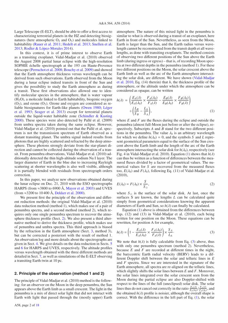
AampA 564 A58 (2014)
Large Telescope (E-ELT) should be able to offer a first access tocharacterizing terrestrial planets in the HZ and detecting biosig-natures (here atmospheric O2 and O3) and molecules linked tohabitability (Rauer et al 2011 Hedelt et al 2013 Snellen et al2013 Rodler amp Loacutepez-Morales 2014)
In this context it is of prime interest to observe Earthas a transiting exoplanet Vidal-Madjar et al (2010) observedthe August 2008 partial lunar eclipse with the high-resolutionSOPHIE eacutechelle spectrograph at the 193 cm Haute-Provencetelescope (Perruchot et al 2008 Bouchy et al 2009) and showedthat the Earth atmosphere thickness versus wavelength can bederived from such observations Earth observed from the Moonduring a lunar eclipse indeed transits in front of the Sun andgives the possibility to study the Earth atmosphere as duringa transit These first observations also allowed one to iden-tify molecular species in the atmosphere that is water vapour(H2O) a molecule linked to Earth habitability biogenic oxygen(O2) and ozone (O3) Ozone and oxygen are considered as re-liable biosignatures for Earth-like planets (Owen 1980 Leacutegeret al 1993 Seager et al 2013) except for terrestrial planetsoutside the liquid-water habitable zone (Schindler amp Kasting2000) These species were also detected by Palleacute et al (2009)from umbra spectra taken during the same eclipse HoweverVidal-Madjar et al (2010) pointed out that the Palleacute et al spec-trum is not the transmission spectrum of Earth observed as adistant transiting planet The umbra signal indeed results fromphotons that are highly scattered and refracted by the deep atmo-sphere These photons strongly deviate from the star-planet di-rection and cannot be collected during the observation of a tran-sit From penumbra observations Vidal-Madjar et al (2010) ad-ditionally detected the thin high-altitude sodium Na I layer Thelarger diameter of Earth in the blue due to increasing Rayleighscattering at shorter wavelengths is also well visible althoughit is partially blended with residuals from spectrograph orderscorrection
In this paper we analyze new observations obtained duringthe lunar eclipse on Dec 21 2010 with the ESO spectrographsHARPS (from asymp3800 to 6900 Aring Mayor et al 2003) and UVES(from asymp3200 to 10 400 Aring Dekker et al 2000)
We present first the principle of the observation and differ-ent reduction methods the original Vidal-Madjar et al (2010)data reduction method (method 1) which makes use of a pair ofpenumbra spectra and a second method (method 2) which re-quires only one single penumbra spectrum to recover the atmo-sphere thickness profile (Sect 2) We also present a third alter-native method to derive the thickness profile which makes useof penumbra and umbra spectra This third approach is biasedby the refraction in the Earth atmosphere (Sect 3 method 3)but can be corrected a posteriori with the result of method 1An observation log and more details about the spectrographs aregiven in Sect 4 We give details on the data reduction in Sects 5and 6 for HARPS and UVES respectively The altitude profilesversus wavelength obtained with the three different methods aredetailed in Sect 7 as well as simulations of the E-ELT observinga transiting Earth twin at 10 pc
2 Principle of the observation (method 1 and 2)
The principle of Vidal-Madjar et al (2010) method is the follow-ing for an observer on the Moon in the deep penumbra the Sunappears above the Earth limb as a small crescent The light in thepenumbra is a mix of direct solar light that did not interact withEarth with light that passed through the (mostly upper) Earth
atmosphere The nature of this mixed light in the penumbra issimilar to what is observed during a transit of an exoplanet hereEarth in front of the Sun Nevertheless as seen from the MoonEarth is larger than the Sun and the Earth radius versus wave-length cannot be reconstructed from the transit depth et all wave-lengths as done with transiting exoplanets The method consistsof observing two different positions of the Sun above the Earthlimb (during ingress or egress) ndash that is of recording Moon spec-tra at two different depths in the penumbra (method 1) For thesetwo different positions on the Moon the solar crescent above theEarth limb as well as the arc of the Earth atmosphere intersect-ing the solar disk are different We have shown (Vidal-Madjaret al 2010 Eq (14) therein) that h the thickness profile of theatmosphere or the altitude under which the atmosphere can beconsidered as opaque can be written
h(λ) =
(EA(λ)EA(λ0)
times FA(λ0)FA(λ)
minus EB(λ)EB(λ0)
times FB(λ0)FB(λ)
)
divide(
LB
S Bminus LA
S A
) (1)
where E and F are the fluxes during the eclipse and outside thepenumbra (almost full-Moon just before or after the eclipse) re-spectively Subscripts A and B stand for the two different posi-tions in the penumbra The value λ0 is an arbitrary wavelengthfor which we define h(λ0) = 0 and the symbols S and L repre-sent geometrical parameters equal to the surface of the Sun cres-cent above the Earth limb and the length of the arc of the Earthatmosphere intersecting the solar disk for h(λ0) respectively (seeFig 4 in Vidal-Madjar et al 2010) Equation (1) shows that h(λ)can thus be written as a function of differences between the mea-sured fluxes divided by a factor of geometrical values The nu-merical values for S are recovered from the measured fluxestoo E(λ0) and F(λ0) following Eq (11) of Vidal-Madjar et al(2010)
E(λ0) = F(λ0) times SS (2)
where S is the surface of the solar disk At last once thesurfaces S are known the lengths L can be calculated quitesimply from geometrical considerations knowing the apparentdiameters of Earth and Sun so h(λ) can finally be calculated
Equation (1) above is obtained from the differences betweenEqs (12) and (13) in Vidal-Madjar et al (2010) each beingwritten for one position on the Moon These equations can berewritten for position A for example
h(λ) =
(1 minus EA(λ)
EA(λ0)times FA(λ0)
FA(λ)
)times S A
LAmiddot (3)
We note that h(λ) is fully calculable from Eq (3) above thuswith only one penumbra spectrum (method 2) Neverthelessbecause E and F are recorded at different times in the nightthe barycentric Earth radial velocity (BERV) leads to a dif-ferent Doppler shift between the solar and telluric lines in Eand F spectra Since we are interested in the signature of theEarth atmosphere all spectra are re-aligned on the telluric lineswhich slightly shifts the solar lines between E and F Moreoverthe solar lines integrated over the solar crescent seen from theMoon during the partial eclipse are also Doppler-shifted withrespect to the lines of the full (uneclipsed) solar disk The solarlines thus do not cancel out correctly in the ratio EA(λ)
EA(λ0) FA(λ)FA(λ0) and
the obtained h(λ) profile is noisier although the overall shape iscorrect With the difference in the left part of Eq (1) the solar
A58 page 2 of 18
L Arnold et al Earth as a transiting exoplanet observed during the 2010 lunar eclipse
lines cancel out much better and the h(λ) profile is cleaner Thisis discussed in more details in Sect 72
3 An alternative method that approximates h(λ)(method 3)
This section describes another method different from that ofVidal-Madjar et al (2010) to derive the thickness profile ofEarth atmosphere In a lunar eclipse the radius of Earth is givenby the radius of the umbra The umbra radius can be calcu-lated geometrically for a solid sphere that casts its shadow to theMoon but in practice the Earth atmosphere that scatters lightalong Earth limb lead to a blurred edge between umbra andpenumbra on the Moon surface The radiance profile across theumbra edge has been measured in the past by several observers(especially by Dubois from 1950 to 1980 Danjon 1925 Combazet al 1950 Reaves amp Walker 1952 Walker amp Reaves 1957) Theirradiance of the eclipsed Moon as well as the umbra edge havealso been modelized (Link 1969 Vollmer amp Gedzelman 2008Garciacutea-Muntildeoz amp Palleacute 2011) by an analysis of the light propa-gation from the Sun to the Moon through the Earth atmosphereThe observed magnitude versus position with respect to the um-bra center looks approximately like a hyperbolic function (orsigmoid) The observations mentioned above indicate that mag-nitude typically drops by about 8 mag from penumbra to umbrathe steepest region being typically 2 arcmin wide (Dubois ampPoumeyrol 1954) Unfortunately the spatial resolution of pub-lished radial photometry across the umbra edge is only about1 arcmin and not sufficient to reveal a dependance of the umbraradius with wavelength To fix the order of magnitude with anEarth umbra radius of asymp43 arcmin a variation of 10 km in theEarth radius (of 6371 km) translates into a change of the umbraradius of 4 arcsec
With ESOrsquos HARPS and UVES spectrographs we recordedspectra from deep penumbra to umbra over asymp7 arcmin withHARPS and asymp19 arcmin with UVES Because the telescopetracked neither the star nor the Moon but the Earth umbra pro-jected to the Moon we were able to integrate the signal at fixeddistances from the umbra edge while the Moon itself slowlyshifted in front of the spectrographs during the exposures Tocompare the flux in these spectra taken at different positions inthe umbra or in the penumbra we calculate their correspondingmagnitude minus25 log10(EF) relative to the full-Moon spectrarecorded before the eclipse Then we plot for each wavelengththe magnitudes versus their distance from the umbra center asDubois did But while Dubois observed at three or four dif-ferent wavelengths through broadband blue green yellow andred Wratten filters HARPS and UVES allow to do this now ata much higher spectral resolution The points follow the sameoverall shape as Duboisrsquo profiles (Fig 1) We fit a hyperbolicfunction through these points
ζ(r) = a0 + a1 tanh[a3(r minus a2)] (4)
where ζ is the model giving the magnitude in the radial direc-tion through the umbra edge r the distance to the umbra centerand ai the parameters defining the hyperbolic function The func-tion ζ(r) varies between a0 minus a1 and a0 + a1 We may arbitrarilydefine the abscissa a2 of the inflection point (at ordinate a0) ofthis function as a measurement of the umbra radius and thus ofthe Earth radius at the observing wavelength
Nevertheless Fig 1 shows that the inflection point corre-sponds to a zone about 3 mag (asymp15times) fainter than shallower
Fig 1 Measured magnitude across the umbra edge with HARPSat 5500 Aring Crosses and diamonds stand for A and B fiber respectivelyThe horizontal error bars are 2σ = 20 arcsec long and represent thetypical pointing error of the telescope Vertically the 2σ error bars arethe magnitude errors evaluated from the SN of the spectra at that wave-length and the evaluated error in the local Moon albedo The solid lineis the model from Eq (4) fitted through the data The vertical dottedline marks our definition of the umbra edge See Sect 73 for details
penumbra But in a real transit only the beams of light that in-teract with the top of the atmosphere and thus only weakly ab-sorbed leave a signature in the transit If a beam goes deeperto the atmosphere it is significantly dimmed and scattered andfinally absent from the transit signature of the planet Thereforethe informations from the 3 mag fainter light we obtain at theinflection point are not those we obtain during a real transit Theinflection point is thus not the best definition of the edge of theEarthrsquos umbra on the Moon at least in the context of our Earth-transit analysis It is more relevant to define a point slightly morein the brighter penumbra for the edge of Earthrsquos umbra as shownby the vertical dotted line in Fig 1 and to build up the Earthradius versus wavelength from this point instead of from theinflection point More details are given in Sect 73
We understand that this method makes use of informationthat is not available in an exoplanet transit indeed it uses in-formation from spectra of the umbra to build the function ζbut as mentioned in the introduction the photons from the um-bra result from highly angularly scattered or refracted beamswhich are not available in the observation of an exoplanet tran-sit Moreover the umbra photons especially the red ones havebeen refracted by the deepest Earth atmospheric layers and theEarth shadow is thus shrunk by refraction at these wavelengthsleading to a smaller Earth radius in the red In other words thegradient in the altitude profiles measured from blue to red wave-lengths will be steeper due to refraction But we show in Sect 73that the altitude profiles h(λ) obtained by this method can becalibrated (scaled) to the profiles obtained with method 1
4 Observing log
HARPS provides spectra with a spectral resolution of 115 000and covers the visible range (Table 1 Mayor et al 2003) UVESwas used in dichroic-1 and dichroic-2 modes (DIC1 and DIC2)
A58 page 3 of 18
AampA 564 A58 (2014)
Table 1 HARPS and UVES spectral ranges
Instrument Range (Aring) Gap (Aring)HARPS 3782ndash6912 5256ndash53375UVES DIC1 BLUE 3055ndash3885UVES DIC1 RED 4788ndash6806 5750ndash5821UVES DIC2 BLUE 3751ndash4999UVES DIC2 RED 6712ndash10 426 8544ndash8646
Notes Gaps without data are present in the final spectra due to smallgaps between detectors
Table 2 Series of n Moon reference spectra taken with HARPS beforethe eclipse
Start Exposure Airmasshminss UT (n times s)021826 4 times 30 215ndash212044120 5 times 45 170
Table 3 HARPS exposures and fiber positions in the penumbra (nega-tive values) and umbra (positive values) with respect to the umbra edgegiven by Guide-9
Start Exposure Fib A Fib Bhminss UT (s) (arcsec) (arcsec)064332 600 ndash66 41065728 450 ndash204 ndash98070635 300 ndash232 ndash125071307 900 36 141
Table 4 Series of three Moon reference spectra taken with UVES be-fore the eclipse
Start Exposure Mode and arm Mean airmasshminss UT (3 times s)020419 3 times 4 DIC2 RED 201020423 3 times 10 DIC2 BLUE 201021849 3 times 4 DIC1 RED 190021856 3 times 40 DIC1 BLUE 190050725 3 times 4 DIC2 RED 156050729 3 times 10 DIC2 BLUE 156051926 3 times 4 DIC1 RED 157051930 3 times 30 DIC1 BLUE 158
In each of these modes both BLUE and RED arms of the spec-trograph are used simultaneously and with standard settingstwo exposures (one in each mode) give a full [3100ndash10 400] Aringspectrum (Table 1 Dekker et al 2000) The slit width was setto 03 arcsec which gives a spectral resolution of asymp120 000
Tables 2 and 3 give information on the observations madefrom La Silla with HARPS The position with respect to theumbra edge was measured with Guide-91 Tables 4 and 5 givethe same information but for UVES at Paranal With UVES thetelescope was not positioned as expected on the Moon during theeclipse and the expected positions are indicated in parentheses inTable 5
As an example we show in Fig 2 the Sun seen from whereHARPS fiber-A was positioned on the Moon at 070635 UTat the beginning of the 300 s exposure (Table 3) The Sun issetting in the Pacific Ocean about 2000 km southeast of Japanat coordinates asymp156 E and asymp23 N The daytime cloud fraction
1 httpwwwprojectplutocom
Table 5 UVES exposures or series of n exposures and measured slitpositions in the penumbra (negative values) and umbra (positive values)with respect to the umbra edge given by Guide-9
Start Exposure Mode and arm Slit positionhminss UT (n times s) (arcsec)064519 2 times 40 DIC1 RED ndash210 (ndash90)064523 180 DIC1 BLUE ndash210 (ndash90)065107 3 times 20 DIC1 RED ndash233 (ndash180)065111 180 DIC1 BLUE ndash233 (ndash180)065801 600 DIC1 RED 577 (360)065805 600 DIC1 BLUE 577 (360)071508 2 times 60 DIC2 RED ndash220 (ndash90)071512 90 DIC2 BLUE ndash220 (ndash90)071935 2 times 25 DIC2 RED ndash229 (ndash180)071939 60 DIC2 BLUE ndash229 (ndash180)072230 20 DIC2 RED ndash147 (360)072234 20 DIC2 BLUE ndash147 (360)073510 600 DIC2 RED 936 (360)073514 600 DIC2 BLUE 936 (360)
Notes The expected slit positions are given in parentheses in the lastcolumn
Fig 2 Earth and Sun seen from the Moon deep penumbra whereHARPS fiber A was positioned at 070635 UT at the beginning ofthe 300 s exposure Image with Guide-9
for 2010 Dec 21 given by AquaMODIS2 for these coordinatesis geasymp07
5 HARPS data processing
The data processing makes use of so-called s1d reduced dataoutput files directly from the HARPS data reduction soft-ware (DRS) The HARPS instrumental response is calibratedwith a high signal-to-noise ratio (SN) G2V star spectrum
51 Correction for the Moon reflectivity
To accurately maintain a given position of the spectrograph withrespect to the umbra edge during the exposures we needed totrack the umbra not the Moon itself The Moon was thus mov-ing in front of the spectrograph pair of fibers at a speed of about055 arcsecs The shift of the Moon during a given exposurecontributed to smooth out any relative spectral reflectance dif-ferences between the lunar terrains that drifted in front of the
2 httpmodisgsfcnasagov
A58 page 4 of 18
L Arnold et al Earth as a transiting exoplanet observed during the 2010 lunar eclipse
Fig 3 Example of a path of the HARPS fibers across the reconstructedMoon image during the 300 s exposure in the penumbra The darkeningfrom the penumbra and umbra are not superimposed on the image heresince we are only interested in recovering the moon reflectivity The Aand B fibers remained at 232 and 125 arcsec from the umbra edge whilethe fibers path across the Moon was asymp164 arcsec long (length of the yel-low lines) The mean reflectivity is measured along the path taking intoaccount a 10 arcsec pointing error in both RA and Dec directions Theterrain reflectivity fluctuates by σ = 21 along the path for Fiber Aand σ = 15 for Fiber B in this highly contrasted lunar region Theerror on the mean reflectivity due to pointing uncertainty is estimatedto be about σ = 4 The figure shows that while Fiber A went throughthe dark region of Mare Nectaris Fiber B remained on a region mea-sured 39 brighter between Catharina and Cyrillus craters pointing outthe relevance of correcting the flux for lunar local reflectivity
spectrograph But different terrains with different albedos wereseen by each fiber during the different exposures To correct eachspectrum for the flux variations induced by these albedo varia-tions we measure the mean lunar reflectivity along the path ofthe slit across the Moon surface during the exposures a poste-riori The path is reconstructed from the date and telescope co-ordinates available in the metadata We build a picture of theMoon as seen during the eclipse from La Silla at a resolutionof 1 arcsecpixel the reconstructed scene is an orthographic pro-jection of a Clementine albedo map3 at 750 nm (Eliason et al1999) and takes into account the correct libration angles thecorrect phase angle (close of zero degree) and a Lambert-Lunarlimb-darkening law (Mc Ewen 1996) The mean lunar reflectiv-ity is then measured with Audela-204 along the path of eachfiber across the lunar surface as shown in Fig 3
52 Correction for the signature of the atmosphereabove the telescope
To correct our eclipse spectra for the signatures of the atmo-sphere above the telescope we need a reference transmissionspectra for the atmosphere T (λ) To derive T (λ) we proceedas in Vidal-Madjar et al (2010) by calculating the ratio oftwo full-Moon spectra F1 and F2 taken before the eclipse atdifferent airmass AM1 and AM2 lt AM1 The ratio can be scaledto AM = 1 following
T (λ) =
[FAM1
1 (λ)
FAM22 (λ)
](1(AM1minusAM2))
middot (5)
We calculate T (λ) with AM1 = 22 and AM2 = 17 (Table 2)Since we are interested only in the accurate measurement of the
3 httpwwwlpiusraedulunartoolsclementine4 httpwwwaudelaorg
Fig 4 La Silla atmosphere transmission function T (λ) for AM = 1 asevaluated from full-Moon spectra taken with HARPS just before theeclipse (Table 2) The spectrum is normalized at 6866 Aring To verifythis experimental T (λ) spectrum a transmission fit based on the modelof Hayes amp Latham (1975) for the Rayleigh and aerosol componentsnormalized at 6866 Aring is displayed (blue dashed line) We also add anozone transmission spectrum to the model (light-blue solid line) thatcorrectly fits the observed wide Chappuis band The best least-squaresfit for Rayleigh and ozone over La Silla that night is obtained for anairmass of AM = 077 for ozone and Rayleigh and an optical depthof 0181 at 5320 Aring for the aerosols between 4000 and 6866 Aring The fitfor ozone is made only where O2 and H2O absorption bands are absentThe O2 γ and B absorption bands are clearly seen around 6300 and6900 Aring respectively the other deep bands are due to H2O The smallgap in HARPS data is visible between 5300 and 5340 Aring (Table 1)
telluric lines in T (λ) the two spectra in Eq (5) are correctedfor the BERV to properly align the telluric lines of both spec-tra (the solar lines become slightly misaligned) Figure 4 showsthe obtained average reference transmission T (λ) that we nowuse in the following data analysis of HARPS data to re-evaluateall eclipse spectra as if they were collected from outside theatmosphere
6 UVES data processing
The UVES instrumental response is calibrated with the referencestar HD 80170 (K5 III-IV Teff = 4537 K log (g) = 21 Randichet al 1999)
61 Correction for the Moon reflectivity
To measure the mean lunar reflectivity along the path ofthe UVES slit across the Moon surface we build a picture ofthe Moon as seen during the eclipse from Paranal as we did forthe HARPS observations An example of the slit path is shownin Fig 5
62 Correction for the signature of the atmosphereabove the telescope
We can not proceed exactly as with the HARPS data be-cause full-Moon spectra show that the water-vapour lines were
A58 page 5 of 18
AampA 564 A58 (2014)
Fig 5 Example of a path of the UVES slit across the reconstructedMoon image during the 600 s exposure in the umbra The slit 10 arcseclong and perpendicular to the path remains at asymp936 arcsec from theumbra edge while the slit path over the Moon was asymp330 arcsec long(length of the yellow line) The mean reflectivity is measured along thepath taking into account a 10 arcsec pointing error in both RA and Decdirections The terrain reflectivity fluctuates by σ = 13 along the pathin this bright lunar region and the error on the mean reflectivity due topointing uncertainty is estimated to be about σ = 4
Fig 6 Part of the spectrum showing the ratio of a high airmass overa low airmass UVES full-Moon spectra The oxygen B and A bandsat 6900 and 7600 Aring respectively are in absorption as expected but thewater vapour bands at 7200 and 8200 Aring appear in emission showingthat the amount of water vapour along the line of sight was higher whenthe airmass was lower indicating that the amount of water vapour aboveParanal increased during the first part of the night before the eclipse Tocalculate this ratio the spectra are aligned by cross-correlation to matchthe radial velocity of the telluric lines so the solar lines do not properlycancel out in the ratio and appear with a wing in emission and the otherin absorption
stronger while the Moon was higher in the sky while it shouldhave been lower for the Moon at a smaller airmass Figure 6indeed shows that the amount of water vapour above the tele-scope increased during the first part of the night between thetwo sets of full-Moon observations We describe below how weconsequently corrected our UVES data
Table 6 Measured PWV before the eclipse and at the end the observa-tion and reduced PWV for airmass =1
hmin UT PWV Airmass PWV (mm) Note(mm) at zenith
0205 and 0218 643 201 320 10508 and 0521 800 156 514 20823 and 0832 595 104 571 3
Notes 1 full-Moon before penumbra ingress DIC2 and DIC1 obser-vations respectively 2 full-Moon before penumbra ingress DIC2 andDIC1 observations respectively First contact with penumbra occurredat about 0528 UTC 3 HD 80170 at the end of the eclipse observationDIC1 and DIC2 observations respectively
We estimate the precipitable water vapour (PWV) in ourspectra by using the spectral-fitting method described in Querelet al (2011) This method compares the measured spectrum witha reference spectrum while varying the reference water-vapourcontent The reference spectrum is generated using an atmo-spheric model configured with the local environmental parame-ters at the time of measurement (ambient temperature pressureelevation etc) A comparison is then made over several smallspectral intervals (asymp2ndash5 nm) where the only significant featuresare caused by absorption by water vapour A least-squares fit isperformed between the measured data and reference spectra for arange of PWV values The reference spectrum with the smallestfit residual represents the water-vapour content (or PWV) mostsimilar to that of the measured spectrum Since this absorptionis along the line-of-sight and assuming an isotropic distributionof water vapour above the telescope the absorption must thenbe corrected back to zenith by dividing the best-fit PWV by theairmass of the measurement
Table 6 indicates that three hours before the eclipsestarted the PWV measured on the full-Moon spectrum wasabout 64 mm for an airmass of 2 The PWV for air-mass =1 was therefore 32 mm Later in the night and justbefore the penumbra ingress we find that PWV increasedto 800 mm at airmass =156 indicating the increase of mois-ture above the telescope The reduced PWV for airmass =1 isthus 800156 = 51 mm before the eclipse started Immediatelyafter the eclipse observations we observed HD 80170 and mea-sured a reduced PWV of 571 mm We therefore assume thatduring the eclipse the PWV at zenith remains within the[51 57] mm range and we chose the mean value 54 mm asthe reference PWV at airmass =1 during the eclipse PWV val-ues of 5 mm are relatively high for Paranal and we understandthat assuming such a high water vapour content is isotropic andconstant above the telescope for three hours (the duration of ourobservations) may be a strong assumption Nevertheless it isthe best we can do and the whole process of data reduction lead-ing to h(λ) assumes the stability of the PWV above Paranal dur-ing the observations (this is obviously also true for the HARPSobservations at La Silla)
To correct our eclipse spectra for the signatures of the atmo-sphere above the telescope we need distinct reference transmis-sion spectra one for water and and one for oxygen In the follow-ing we describe how these reference spectra are obtained Thesereference transmission spectra do not need to include Rayleighand ozone signatures because they are already corrected for byUVES reduction pipeline
The UVES transmission water-vapour spectrum TH2O(λ) forairmass =1 (PWV = 54 mm) is obtained by the ratio of the
A58 page 6 of 18
L Arnold et al Earth as a transiting exoplanet observed during the 2010 lunar eclipse
full-Moon spectra F for which we know the value of PWV(Table 6)
TH2O(λ) =(F(PWV = 800)
F(PWV = 643)
)54(800minus643)
middot (6)
To derive a spectrum for pure water vapour (ie without thelines from other elements or molecules) TH2O(λ) is calculatedonly when water-vapour absorption is present (T le 99) inthe water-vapour synthetic spectrum computed to measure thePWV To avoid TH2O(λ) to become too noisy in the deepest ab-sorption bands of water vapour the spectrum is not calculatedwhen water-vapour transmission becomes T le 25
The transmission spectrum for O2 for airmass =1 is obtainedby taking into account the variation of airmass AM between thetwo F spectra (Table 6) as done by Vidal-Madjar et al (2010)
TO2(λ) =(F(AM = 201)
F(AM = 156)
)1(201minus156)
middot (7)
And as for TH2O TO2 is calculated only when O2 absorption ispresent (999 ge T ge 2) in a AM = 1 MODTRAN5 syntheticspectrum
Once TH2O and TO2 are known we can correct our spectrasimply by the division
s =S
(TH2O times TO2 )AM (8)
where s is the corrected spectrum and S is a full-Moon or eclipsespectrum acquired at airmass AM The final T (λ) spectrum forParanal is shown in Fig 7 The continuum shows neither theRayleigh nor the ozone signature in this spectrum (on the op-posite of what is obtained with HARPS Fig 4) because theUVES reduction pipeline automatically removed from all spec-tra tabulated values for the Rayleigh and ozone signatures at thecorresponding airmass of the observation Of course the addi-tional Rayleigh and ozone signatures present in the eclipse spec-tra and produced by the light path through the limb of the Earthatmosphere have not been removed by the UVES pipeline
To calculate TH2O and TO2 the full-Moon spectra are alignedwith a cross-correlation to match the radial velocity of thetelluric lines
7 Results and discussion
71 Results from Eq (1) (method1)
From the HARPS data we build five pairs of penumbra spectrasuitable for Eq (1) [98 204] [125 232] [66 125] [66 204]and [66 232] where the numbers in brackets are the positionsdescribed in Table 3 The possible pair [66 98] is not used itproduces a significantly noisier altitude profile probably becausethe positions in the penumbra are too close and the differencebetween the spectra is too small
The penumbra spectra are affected by the wavelength-dependent solar limb darkening LD(λ) (Hestroffer amp Magnan1998) Equation (1) makes use of geometrical parameters Sand L for two different solar crescents visible above Earth Thesolar LD(λ) makes the crescents fainter than the mean solarbrightness The size of the solar crescents estimated from thepenumbra spectra fluxes is thus underestimated if the penum-bra fluxes are not corrected for the solar LD To correct for
5 httpmodtran5com
Fig 7 Paranal atmosphere transmission function T (λ) for AM = 1 asevaluated from full-Moon spectra taken with UVES before the eclipsefollowing the reduction process described in Sect 62 The UVES re-duction pipeline automatically removes from all individual spectra tab-ulated values for the Rayleigh aerosol and ozone signatures at the cor-responding airmass of the observation These signatures therefore donot appear here as for HARPS (Fig 4) A weak residual curvature ofthe continuum (asymp5 maximum at 7800 Aring with no resemblance to aresidual signature of ozone or Rayleigh) was fitted with a second-orderfunction The spectrum shown here is normalized to this fit to have a flatcontinuum at 1 (horizontal line) The O2 γ A and B bands are clearlyseen (in red) the other bands are due to H2O (in blue)
this effect we first evaluate the size of the solar crescents (pa-rameters S and L) from the flux ratio (penumbrafull-Moon)at λ = 57988 Aring which allows us to evaluate an average LDthat affects each solar crescent following Hestroffer amp Magnan(1998) For these crescent sizes and the LD obtained at λ =57988 Aring a wavelength-dependant limb darkening LD(λ) is thenre-evaluated from the low spectral resolution model of Hestrofferamp Magnan (1998) It covers the spectral ranges [3033ndash3570]and [4160ndash10 990] Aring with a spectral resolution of a few tens(we do a linear interpolation between 3570 and 4160 Aring) Themodel is then used to calculate the LD-corrected penumbra spec-tra EA(λ)LD(λ) and EB(λ)LD(λ) from which new S and L areevaluated for λ0 with Eq (2) Equation (1) is then evaluatedagain to derive the final h(λ) profile
The mean altitude profile from the five pairs of fibers ob-tained from Eq (1) is shown in Fig 8 The profile is shiftedupward by asymp30 km to have an altitude of 238 km in the[4520ndash4540] Aring domain as predicted by Ehrenreich et al (2006)The profile shows the large bump due to ozone Chappuis bandcentered around 5900 Aring and peaking here at about 38 kmand the oxygen γ and B bands at 6300 and 6900 Aring respec-tively Water vapour also appears around 6500 Aring at an altitudeabove 25 km The increase of h(λ) in the blue due to Rayleighscattering is visible as a negative slope between 4000 and 5000 Aring(Ehrenreich et al 2006 Kaltenegger amp Traub 2009) The bluepart of the profile shows many residual solar absorption linesthat bias the binned profile towards lower altitudes Numeroussolar lines are visible for example Hβ at 4861 Aring and Hα at6563 Aring The Fig 9 is a zoom on the Na I doublet The asymp2 Aring-wide
A58 page 7 of 18
AampA 564 A58 (2014)
Fig 8 Altitude profile with HARPS as obtained from Eq (1)(method 1) A 10 Aring bin is superimposed in light-blue over the full-resolution profile The profile shows the large bump due to ozoneChappuis band around 6000 Aring the oxygen γ- and B-band at 6300 at6900 Aring respectively and also the water-vapour band around 6500 AringThe expected increased of h(λ) in the blue due to Rayleigh is visible asa negative slope between 4000 and 5000 Aring Oxygen and water-vapourabsorption spectra at arbitrary scale are shown
photospheric wings of the solar Na lines are still visible Thepresence of all these solar features indicates that the solar sig-nature is not properly removed from the h(λ) profile This couldresult from the EF ratios in Eq (1) The penumbra spectra Eindeed contain the spectrum from the solar crescent that isthe edge of the Sun where solar absorption lines are deeperthan in full-Moon spectra F which correspond to a full disk ofthe Sun illuminating the Moon We therefore tried to adjust apower p gt 1 on F to compensate for the solar residuals with ra-tios E(F p) in Eq (1) instead of EF But we found p to be veryclose to 1 and could not detect a significant difference betweenthe average depth of the absorption lines in E and F
Vidal-Madjar et al (2010) observe the same type of solarresiduals in the SOPHIE data (residual wings of the Na I dou-blet) and the explanation invoked is the Ring effect The depthof solar Fraunhofer lines in scattered light is lower than in di-rect sunlight This effect is known as the Ring effect (Graineramp Ring 1962) and is mainly induced by rotational Raman scat-tering (Vountas et al 1998) The line filling-in for forwardscattering (as experienced by the photons that interact withthe Earth atmosphere and are scattered towards the eclipsedMoon) is about 21 and 38 of the continuum for single andmultiple scattering respectively for the Ca II K line (Vountaset al 1998) Kattawar et al (1981) report a filling-in of 25at 63015 Aring for a Fe-I line Brinkmann (1968) calculates afilling-in of about 17 in the center to 19 in the wings fora hypothetical line at 4000 Aring underlining the continuous andsmooth effect across the line profile which is also measured byPallamraju et al (2000) Brinkmann (1968) reports observationsshowing a decrease of the filling-in with wavelength by a factorof 2 between 4383 and 6563 Aring and more recent measurements(Pallamraju et al 2000 Fig 3 therein) shows that the Ring effectdecreases approximately linearly by a factor of asymp3 from 4285
Fig 9 Zoom in the Na I doublet region of the altitude profile from Fig 8with HARPS and method 1 The asymp2 Aring-wide photospheric wings of theNa lines are still present showing that the solar signature is not properlyremoved from this h(λ) profile A residual solar line of Ni I is visibleat asymp58929 Aring (Wallace et al 2011)
to 6560 Aring for a given line strength (normalized depth to contin-uum times width)
Several methods exist to correct for the Ring effect (Wagneret al 2001) The simplest is that of Noxon et al (1979) whichconsists of subtracting a small constant close to 2 from thespectrum This was the solution applied in Vidal-Madjar et al(2010) where a constant is empirically adjusted to remove theresidual solar Na I lines (the constant was 4 and 06 of thecontinuum in the Na I region for the deepest and the shallowestpositions in the penumbra respectively) We also correct thisRing effect in our data
We observed that removing a Ring value xa from the shal-lowest spectrum in the penumbra and xb(gtxa) to the deepestspectrum gives almost the same result as removing xb minus xa tothe deepest only (all spectra were corrected from the instrumen-tal response so Noxonrsquos approach applies correctly) The Ringsignature is thus as expected stronger in the deeper spectrum(xb gt xa) where collected photons have been more scatteredin Earth atmosphere than photons collected in the shallowerpenumbra In our empirical correction for the Ring effect wetherefore only apply a correction on the spectrum in the deepestposition in the penumbra We consider empirical Ring correc-tions following i) Noxon et al (1979) ii) Noxon et al (1979)except in deep telluric bands (T lt 05) where the Ring effectis negligible because Raman-scattered photons are strongly ab-sorbed (Sioris amp Evans 2000) iii) a λminus2 power law to mimicthe chromatic dependance observed by Pallamraju et al (2000)or Brinkmann (1968) iv) a λminus2 power law subtracted except indeep telluric bands (T lt 05) and v) a subtraction of the recip-rocal of the spectrum (Johnston amp McKenzie 1989) that mimicsthe Ring spectrum Here again the obtained Ring spectrum isnot removed from deep telluric lines (T lt 05)
We observe that removing asymp1 of the continuum at 5880 Aringto the deepest spectrum of each pair reduces the solar residualsover the full altitude profile (Fig 10) and slightly reduces the
A58 page 8 of 18
L Arnold et al Earth as a transiting exoplanet observed during the 2010 lunar eclipse
Fig 10 Altitude profile with HARPS and method 1 without Ring cor-rection (upper panel) and different empirical Ring corrections Theamount of correction is 1 of the continuum at 5880 Aring i) Noxon et al(1979) ii) Noxon et al (1979) except in deep telluric bands (T lt 05)where the Ring effect is negligible because Raman-scattered photonsare strongly absorbed (Sioris amp Evans 2000) iii) a λminus2 power law tomimic the chromatic dependance observed by Pallamraju et al (2000)or Brinkmann (1968) iv) a λminus2 power law subtracted except in deeptelluric bands (T lt 05) and v) a subtraction of the reciprocal of thespectrum (Johnston amp McKenzie 1989) which mimics the Ring spec-trum Here again the obtained Ring spectrum is not removed from deeptelluric lines (T lt 05) The Na I doublet peaks at asymp5890 Aring for all typesof Ring corrections tested
Na wings (Fig 11) The correction also leads to the rise of theNa lines to altitude values of asymp80 km a value in agreement withthe literature (Plane 2003 Moussaoui et al 2010) Neverthelessthe width of the terrestrial Na I peaks are observed to be asymp04 AringThis is larger than the asymp02 Aring observed for the other tel-luric lines but might be induced by the presence of the strongNa I line in the solar spectrum The extraction process of h(λ) isthen more disturbed in the case of the Na I lines easily induc-ing a change in the width particularly because the solar linescannot be perfectly positioned in all spectra since these havebeen Doppler-shifted to have the telluric lines aligned An addi-tional effect is the limb-darkening effect that changes the shapeof the solar Na I lines emitted by different size crescent above theEarth limb This is also why the broad Na I stellar wings are notperfectly corrected in the presented extraction procedure whichonly includes a low spectral resolution limb-darkening modelFinally we also note that only the Na I lines are detected inFig 10 not the strong Mg I triplet at asymp5170 Aring nor Hα for
Fig 11 Same as Fig 10 but zoomed-in on the Na I doublet region ofthe altitude profile without Ring correction (upper panel) and differentempirical Ring corrections
example produce a peak in the altitude profile We thereforeconclude that the terrestrial Na layer is detected
Interestingly Garciacutea-Muntildeoz et al (2012) point out that thelunar eclipse of 16 August 2008 occurred only four days after themaximum of the Perseid meteor shower It is indeed known thatmeteor showers can temporarily increase the amount of sodiumin the atmosphere by a factor up of 10 (Plane 2003 Moussaouiet al 2010) This corroborates the detection of the sodium layerby Vidal-Madjar et al (2010) in August 2008 Nevertheless theGeminid meteor shower maximum occurs on December 13 Itis an active meteor shower with a particle density similar tothat of the Perseids6 that might have increased the sodium ab-sorption during the eclipse of 21 December 2010 Neverthelessour observations just show that the Na layer is indeed presentas during our first observations in August 2008 Since we haveonly one measurement it is unfortunately not possible to detectany change of the atmospheric Na I content either in 2008 orin 2010 and thus to confirm a link with any meteor shower
It can be seen from Fig 10 that the Ring correction is nothomogeneous across the full spectral range the Hα line remainsundercorrected while lines in the bluer part of the h(λ) pro-file are overcorrected We therefore adopt the simplest Noxon
6 See for example the IMO (International Meteor Organization)data at httpwwwimonetlivegeminids2012andhttpwwwimonetliveperseids2012
A58 page 9 of 18
AampA 564 A58 (2014)
Fig 12 Final altitude profile obtained with HARPS method 1 and with a Noxon correction for the Ring effect expect in the deep telluric lines(Sioris amp Evans 2000) A 10 Aring bin is superimposed in light-blue over the full-resolution profile 30 and 100 Aring bins are shown too shifted upwardsfor clarity The Na I peaks are visible near 5900 Aring Oxygen and water-vapour absorption spectra at arbitrary scale are shown The altitude profilehas been shifted to have an altitude of 238 km in the [4520ndash4540] Aring domain as predicted by Ehrenreich et al (2006) (dots and dashes in green ndashdashes to improve the visibility of the curve around 6000 Aring)
approach a subtraction of a constant except in deep telluriclines (T lt 05) The final result and the model from Ehrenreichet al (2006) are shown in Fig 12 The model is flatter than theobserved profile which peaks at about 35 km near 6000 Aring about8 km above the model This difference might be a refraction ef-fect that amplifies the observed profile as with method 3 al-though this effect is weaker here because we use only penum-bra spectra If the profile is calculated only with the two pairs[98 204] and [125 232] (Table 3) leaving out the spectrumfrom the deepest penumbra at only 66 arcsec from the umbrathe observed profile is indeed flatter (but noisier) it still peaksat 35 km higher that the altitude expected from the model butthe lowest altitude at 6900 Aring becomes asymp17 km instead of 12We note that our observations of the 2008 eclipse agrees bet-ter with the model (Vidal-Madjar et al 2010 Fig 9 therein) al-though SOPHIE fibers were between asymp100 and 250 arcsec fromthe umbra edge as for HARPS The additional bins in Fig 12show that the B-band is barely detectable in the 30 Aring bin whilethe broad O3 Chappuis band and Rayleigh slope in the blue re-main visible in the 100 Aring bin Figure 13 shows zooms in theNa I lines and the O2 γ and B band regions Oxygen shows upvery clearly with peaks reaching h = 35ndash40 km Some water-vapour peaks are visible but weak which is not surprising be-cause of the high altitude at which they are detected and alsobecause of the lower strength of the water-vapour absorption inthe HARPS wavelength range compared with λ gt 7000 Aring Wedetect neither Li (6708 Aring) nor Ca II (Hunten 1967 Plane 2003)
With UVES the coordinates of the telescope indicate that thetelescope unfortunately did not move in the penumbra betweenthe exposures in order to record spectra at 90 and 180 arcsecfrom the umbra edge as expected but instead stayed asymp200 arcsecfrom the umbra (Table 5) The different recorded spectra arevery similar and the result from Eq (1) is noisy especially inthe blue Residuals from spectral orders are also visible above7000 Aring There is nevertheless a spectrum taken in UVES DIC2
configuration while the telescope was thought to be in the um-bra but was too close to the Moon edge and left the moon about20 s after the exposure started The exposure was then stoppedbut the telescope coordinates indicate that the telescope was infact in the penumbra The exposure time for that unexpected ex-posure is only about 21 and 38 of what was required for theBLUE and RED exposures respectively The altitude profile ob-tained with UVES is shown in Fig 14 The overall shape agreeswith the model of Ehrenreich et al (2006) but the altitude ob-served in the UV is far higher than that of the model Moreoverwe had to shift the DIC1 BLUE profile by ndash110 km to connectit to the DIC2 BLUE profile The DIC2 RED profile has also tobe shifted by 35 km to be connected to the altitude obtained forthe DIC1 RED profile The oxygen bands are barely visible andthe water-vapour bands appears in absorption We did not con-sider any Ring correction for this noisy profile Note also thatthe model of Ehrenreich et al (2006) shown in the figures of thispaper does not include water vapour
72 Results from Eq (3) (method 2)
The HARPS spectra are now used with Eq (3) to calculate hfrom only one penumbra spectrum The eclipse spectra are cor-rected for limb-darkening and Ring effect as for method 1 Whenthe profile is calculated with the spectra in Eq (3) aligned onthe telluric lines the solar lines become consequently slightlymisaligned which generates noise in the profile (Fig 15 upperpanel) We therefore build a composite profile where all linesndash telluric and solar ndash are aligned The composite uses two dif-ferent profiles one aligned on the telluric lines and a secondaligned on the solar line In the first profile every misalignedsolar line is recognized with the help of a synthetic G2 spec-trum and replaced by its aligned residual taken from the secondprofile Some solar lines are missing in the G2 spectrum in themost crowded telluric bands therefore some residual noise due
A58 page 10 of 18
L Arnold et al Earth as a transiting exoplanet observed during the 2010 lunar eclipse
Fig 13 Zooms on the HARPS final altitude profile from method 1(Fig 12) with a Noxon correction for the Ring effect except in the deeptelluric lines (Sioris amp Evans 2000) Oxygen and water vapour absorp-tion spectra at arbitrary scale are shown Oxygen shows up very clearlyWater vapour is barely visible around 6500 Aring above 25 km and weaklines are visible in the higher Na I D1 D2 region Note that our Noxoncorrection does not completely remove the wings of the Na I solar linesThe wings disappear with a stronger correction but the two Na I peaksthen reach an altitude well above 100 km which is not realistic
to uncorrected solar lines is still present in the composite in-side these telluric bands The procedure still slightly cleans the hprofile (Fig 15 lower panel) The overall shape of the profileis similar to the profile obtained with Eq (1) shown in Fig 12Ozone appears about 6 km above the model When zooming-in (Fig 16) only the oxygen B and γ bands are correctly de-tected with peaks reaching h = 35ndash40 km Water-vapour bandsat 6500 and 5890 Aring are not visible nor the atmospheric Na I D-lines which are maybe hidden in the strong solar residual linesNote that the profile shown here is for the deeper position in thepenumbra The other positions lead to a noisier result althoughthe overall shape is correct
Equation (3) is also applied on UVES spectra to calculate hAs for HARPS we compute a composite profile The compositeis the profile obtained with the spectra aligned on the solar linesin which the oxygen and water-vapour lines are replaced by theoxygen and water-vapour lines picked up in the profile obtainedwith the spectra aligned on the telluric lines This procedurecleans the profile (Fig 17 lower panel) although compromisingthe detection of atmospheric species different from oxygen andwater This may explain at least partially why the Na I D-linesdo not appear clearly The oxygen γ B and A bands are visibleup to asymp80 km (zooms in Fig 18) but water-vapour bands arenot detected We subtract a Ring effect from the UVES eclipse
Fig 14 Final altitude profile obtained with UVES and method 1 NoRing correction is applied A 10 Aring bin is superimposed in light-blueon the full-resolution profile Reference oxygen and water-vapour ab-sorption spectra obtained with UVES are shown at arbitrary scale Thealtitude profile has been shifted to have an altitude of 238 km in the[4520ndash4540] Aring domain as predicted by Ehrenreich et al (2006) (greendashed line no water vapour in the model)
Fig 15 Altitude profile with HARPS and Eq (3) (method 2) Only thespectrum of the deepest penumbra taken at 66 arcsec from the um-bra is used here (Table 3) Shallower penumbra spectra give similar butnoisier profiles A 10 Aring bin is superimposed in light-blue on the full-resolution profiles The upper panel shows the profile obtained withthe HARPS spectra aligned on the telluric lines Solar lines are conse-quently slightly misaligned and generate noise in the profile The lowerpanel shows a composite profile showing the profile calculated with thespectra aligned on the telluric lines expect when a solar line is presentwhere the profile from spectra aligned on the solar lines is used Oxygenand water-vapour absorption spectra at arbitrary scale are shown Thegreen dashed line is the model of Ehrenreich et al (2006)
A58 page 11 of 18
AampA 564 A58 (2014)
Fig 16 Zooms on the HARPS altitude profile from method 2 shown inFig 15 Oxygen and water-vapour absorption spectra at arbitrary scaleare shown to facilitate the identification of the spectral lines Oxygenis correctly detected while water vapour is not detected AtmosphericNa I D-lines are not detected either maybe they are hidden by the strongsolar residual lines
spectra of 05 of the continuum at 5880 Aring When we subtracta Ring effect of 1 as we did for HARPS the profile does notchange except from the oxygen A and B bands which peak at150 km
Qualitatively speaking the overall shape of the profile from3000 to 7000 Aring is in acceptable agreement with the model withthe ozone Chappuis bump at 6000 Aring and a Rayleigh increaseof h in the blue and near UV The DIC2 BLUE altitude is setto h = 238 km in the [4520ndash4540] Aring domain as predicted byEhrenreich et al (2006) The other parts of the profile need to beshifted by about plusmn6 km to be properly continuously connectedto the DIC2 BLUE profile
73 Results from the umbra edge radiance profile(method 3)
With method 3 we make use of all available umbra and penum-bra spectra The penumbra spectra are corrected from the limb-darkening in the same way as for method 1 and 2 For each sam-pled wavelength in the HARPS spectra we fit a sigmoid curve(Eq (4)) through the eight available measured points (positionmagnitude) in the umbra and deep penumbra region (Table 3)An example of the obtained fit is shown in Fig 1 We now needto define the radius of the umbra edge re from which we build
Fig 17 Altitude profile with UVES and method 2 A 10 Aring bin is su-perimposed in light-blue on the full-resolution profile The upper panelshows the profile obtained with the UVES spectra aligned on the telluriclines with solar lines consequently slightly misaligned and thus gener-ating noise in h The lower panel shows a composite profile showingthe profile aligned on the solar lines when no telluric line is presentand the profile aligned on the telluric lines when a telluric line ispresent Oxygen and water-vapour absorption spectra at arbitrary scaleare shown to facilitate the identification of the spectral lines The modelof Ehrenreich et al (2006) is shown in green
the Earth atmosphere thickness h(λ) simply given by
h(λ) = re(λ) times roplusru+ cte (9)
where re is expressed in arcmin ru = 427 arcmin is the umbraradius from the ephemeris and roplus = 6371 km is the Earth radiusThe constant cte is set to give h = 238 km at [4520ndash4540] Aring
As explained in Sect 3 the inflection point abscissa a2 of thefit is not the best estimate of re (in our context of Earth transitanalysis at least) To explore the impact of re on h(λ) we write resuch that
ζ(re) = a0 + c times a1 (10)
For the inflection point the coefficient c in front of half-amplitude a1 of the tanh function is c = 0 and ζ(a2) = a0Positive values of c lead to positions on the penumbra side ofthe inflection point Figure 19 shows a set of altitude profilesbuilt for different positions across the umbra edge with minus06 ltc lt 09 as shown in Fig 20 The profiles versus c change sub-stantially for c = minus06 the profile is built from data on theumbra side of the inflection point and the bump from the ozoneChappuis band is almost invisible The mean negative slope ofthe profile also underlines the effect of refraction that shrinksthe Earth umbra at redder wavelengths This effect decreaseswhen c increases to positive values with the profiles built fromdata on the penumbra side of the inflection point The broadChappuis band is detected We finally define the umbra radiussuch as ζ(re) = a0 + 06 times a1 (c = 06) For this value thenoise in the altitude profile is close to minimum and the biasfrom shallow umbra (that is the mean negative slope of h(λ))is reduced With this definition Fig 20 puts the umbra edge at
A58 page 12 of 18
L Arnold et al Earth as a transiting exoplanet observed during the 2010 lunar eclipse
Fig 18 Zooms on the oxygen A and B-band regions of the UVES profilshown in Fig 17 (method 2) An oxygen absorption spectrum at arbi-trary scale is shown
about 1 arcmin in the penumbra side with respect to the inflec-tion point and about one magnitude fainter than the penumbraat 4 arcmin from the inflection point This choice is consistentwith our reasoning developed Sect 3
The result with HARPS and method 3 is shown in Figs 21and 22 Wide and narrow features of the Earth atmosphereare visible (Rayleigh ozone Chappuis band oxygen γ andB-bands) Water vapour is not detected suggesting it is notpresent above 12 km Compared with the profile obtained withmethod 1 (Fig 12) the profile with method 3 shows a strongernegative slope from blue to red leading to an altitude rangeabout asymp33 times larger than with method 1 We attribute thiseffect to the fact that method 3 makes use of umbra spectra Thelight in the umbra is reddened by Rayleigh scattering in the deepEarth atmospheric layers and refracted towards the umbra centerTherefore the umbra edge in red light is more refracted towardsthe umbra center than at blue wavelengths The umbra radius(Earth radius on the Moon) is thus smaller in the red than in the
Fig 19 Altitude profiles obtained with HARPS and method 3 for differ-ent positions across the umbra edge given by parameter c in Eq (10)and shown in Fig 20 The vertical axis is the measured altitude setto 238 km at at [4520ndash4540] Aring for the profile calculated for c = 0Other profiles are shifted vertically for clarity by steps of 40 km Theprofiles in this figure are not built at HARPS native resolution but at asmaller asymp06 Aringpixel resolution The light-blue lines are 10 Aring bins
Fig 20 Positions across the umbra edge used to build the altitudeprofiles shown in Fig 19 The positions are defined by parameter c(Eq (10)) and ranging from c = minus06 to 09 The definition for theumbra edge is taken for c = 06 (vertical solid line) at asymp1 arcmin inthe penumbra side with respect to the inflection point here fixed at ab-scissa =0 The umbra edge is only about one magnitude fainter than thepenumbra at 4 arcmin from the inflection point
A58 page 13 of 18
AampA 564 A58 (2014)
Fig 21 Altitude profile obtained with HARPS and method 3 The left vertical axis is the measured altitude set to 238 km at at [4520ndash4540] AringThe right vertical axis is the corrected altitude if one considers the lowest region of h close to altitude 12 km as in Fig 12 and again h = 238 kmat [4520ndash4540] Aring The horizontal dotted line represents the altitude 238 kmThe light-blue line is a 10 Aring bin superimposed on the full-resolutionprofile Oxygen and water-vapour absorption spectra at arbitrary scale are shown
Fig 22 Zooms on the HARPS altitude profile from method 3 shown inFig 21 The left vertical axis is the measured altitude set to 238 km at[4520ndash4540] Aring The right vertical axis is the corrected altitude if oneconsiders the lowest region of h close to altitude 12 km as in Fig 12and again h = 238 km at [4520ndash4540] Aring Oxygen and water-vapourabsorption spectra at arbitrary scale are shown Water vapour is not de-tected above 16 km suggesting that the amount of water vapour is toolow to absorb enough to be visible at this altitude The sodium layerNa I is not detected
Fig 23 Measured magnitude across the umbra edge with UVESat 10 000 Aring The horizontal error bars are 20 arcsec long and repre-sent the typical pointing error of the telescope Vertically the 2σ errorbars are the magnitude errors given by the UVES pipeline and the eval-uated error in the local Moon albedo The solid line is the model fromEq (4) fitted through the data with parameter a3 set to the mean valueof a3 found for the HARPS data The vertical dotted line marks the edgeof the umbra following our definition
blue due to refraction and Rayleigh scattering This effect am-plifies the measured altitude range across the full visible spec-trum To correct for this effect the right vertical axis of Fig 21is calibrated with the method 1 result by setting the altitude fortwo different points that is the lowest region of h at altitude12 km and h = 238 km at [4520ndash4540] Aring
A58 page 14 of 18
L Arnold et al Earth as a transiting exoplanet observed during the 2010 lunar eclipse
Fig 24 Altitude profile obtained with UVES and method 3 The left vertical axis is the measured altitude set to 238 km at [4520ndash4540] Aring Theright vertical axis is the corrected altitude if one considers the lowest region of h close to altitude 0 km and again h = 238 km at [4520ndash4540] AringThe horizontal dotted line represents the altitude 238 km A 10 Aring bin is superimposed in light-blue on the full-resolution profile and a 100 Aring binin red is also shown shifted upwards for clarity The profile for λ le asymp4300 Aring is not shown because the very weak umbra signal induces noise inthe altitude profile which becomes noisy and h unexpectedly decreases Oxygen and water-vapour absorption spectra at arbitrary scale are shown
We process the UVES data in the same way Neverthelesssince we have less observations points with UVES than withHARPS it is not possible to keep four free parameters forthe fitting function the sigmoid ζ We have to fix the a3 pa-rameter to the mean value obtained with HARPS The param-eter a3 describes the steepness of the fit near the inflectionpoint and is quite stable for HARPS at visible wavelengths inthe [6500ndash6900] Aring range its average value is a3 = 988 times 10minus3
with an RMS of σ = 22times10minus4 We fix a3 to that mean value forUVES An example of the fit through the UVES observationsat 10 000 Aring is shown in Fig 23 Figure 24 shows the altitudeprofile obtained with UVES showing the same features as forHARPS with clear oxygen A and B bands and water-vapourbands up to 10 000 Aring As with the HARPS profile (Fig 21) theprofile obtained with UVES displays a strong global negativeslope Here the profile is asymp45 times larger than with method 1The right axis in Fig 24 is calibrated considering that the lowestregion of h is close to altitude 0 km and again that h = 238 kmat [4520ndash4540] Aring The factor of 45 is larger than with HARPS(asymp33) maybe because the slit positions with UVES are deeperin the umbra than with HARPS (see Tables 5 and 3)
In the blue (λ le asymp4300 Aring) the signal in the umbra spectrais weak and the altitude profile becomes noisy and unexpectedlydecreases (this part of the profile is not shown in Fig 24) Theweak signal in the deepest lines of oxygen A-band and watervapour (asymp9300ndash9500 Aring) in the umbra spectra is also responsi-ble for spikes above 100 km at these wavelengths To cancel outmost of these spikes we set a flux threshold for the umbra spec-tra of 1 of the continuum below which the algorithm does notevaluate h At last to have h = 238 km at [4520ndash4540] Aring wesubtract 37 km from the DIC2 BLUE profile To have all parts ofthe profile connected in Fig 24 we shift the DIC1 RED profileby ndash23 km and the DIC2 RED profile by +25 km
The Figs 25 and 26 show zooms in the UVES full profileshown in Fig 24 In Fig 25 the three oxygen bands are clearly
detected Note that the core of the oxygen line for the A-bandcould not be calculated because the signal in the line core is tooweak The sodium layer is not detected and no water vapourappears above 19 km near the sodium lines At λ gt 7000 Aringin Fig 26 water vapour appears very well even at an altitudehigher than 20 km because the water-vapour absorption bandsbecome stronger in these longer wavelengths Water vapour in-deed presents a vertical distribution in the Earth atmosphere andis thus also present at higher altitudes but with lower volumedensities The altitude at which it is detected (where an opticalthickness of about 1 is reached for a grazing line of sight) is ofcourse higher in the stronger bands
It is worth noting that the residuals of the Na I lines are verysimilar apart from the noise for HARPS and UVES (Figs 22and 25 respectively) This is expected because HARPS andUVES observed roughly the same solar crescents and thus expe-rienced the same Doppler shift of the solar lines of the crescentsthat induced these residuals in the altitude profile Note also thatno correction of the Ring effect is implemented in method 3 ei-ther for HARPS or UVES All spectra are indeed used here allat different depths in the penumbra and umbra A simple empiri-cal approach cannot reasonably be considered A physical modelof the Ring effect is much needed taking into account the pathlength through the Earth atmosphere for the different positionsobserved in the umbra and penumbra
74 Possibilities with a future giant telescope
We analyze how our results can be extrapolated to what a futureground-based giant telescope might be able to detect in the visi-ble transmission spectrum of an Earth-like exoplanet observedin transit We use a full model of the future E-ELT a 39 mtelescope The focal instrument has the same throughput pixelsampling and detector characteristics as the EPICS instrumentsThe model takes into account the photon noise from the starthe thermal and readout detector noises the zodiacal noise and
A58 page 15 of 18
AampA 564 A58 (2014)
Table 7 Transit of an Earth twin at 10 pc observed for 8 h by the E-ELTat low spectral resolution and assuming no atmospheric perturbations
Filter λ range h SN δ h plusmn 1-σ(Aring) (km) error (km)
O3 + Rayl 1 5000ndash5500 199 113 172 plusmn 30O3 + Rayl 2 5500ndash6100 192 123 165 plusmn 29O3 + Rayl 3 6300ndash6800 150 86 123 plusmn 29O2-B 6865ndash6905 176 25 148 plusmn 64Rayl 4 7360ndash7560 89 31 62 plusmn 32O2-A 7590ndash7650 232 37 205 plusmn 59Rayl 5 7750ndash8100 72 33 45 plusmn 29Rayl 6 8450ndash8800 53 23 26 plusmn 28Water vapour 9300ndash9600 87 31 60 plusmn 32Window 10 100ndash10 400 27 10 0 plusmn 26
Notes The SN is calculated through ten different filters The last fil-ter ldquoWindowrdquo is for the atmospheric window The filter widths rangefrom 40 Aring for the O2 B to 600 Aring for one of the filter sampling theChappuis band The values of h are taken from the 10 Aring bin of theUVES profile (Fig 24) The value δh is the altitude difference to theatmospheric window measured by the E-ELT
the absorption of the local atmosphere above the telescope (seeHedelt et al 2013 for a detailed description of the model)
We define a set of ten filters i) to sample the Chappuis bandand the Rayleigh continuum and ii) to isolate the most interest-ing narrow features in the profile shown in Fig 24 that is theoxygen A and B bands and the water vapour around 9500 AringThe low spectral resolution 10 Aring bin in this figure shows thatthe oxygen A-band peaks about 20 km above the lowest altitudearound 10 200 Aring The Earth radius is thus 03 larger andthe transit 06 deeper through a filter that isolates the oxy-gen A-band The Earth transit depth is 83 times 10minus5 and the tran-sit variation at that spectral resolution for the O2 band repre-sents 75 times 10minus7 of the stellar flux
According to Porto de Mello et al (2006) there are 33 solar-type stars within 10 pc 13 of which are reasonably similar tothe Sun in terms mass age metallicity and evolutionary sta-tus Considering that the transit probability of an Earth twin infront of its star is about 1 we understand that the probabil-ity of detection is low even if all stars have a planet in theirhabitable zone The Darwin All Sky Star Catalogue (Kalteneggeret al 2010) lists 878 single FGK stars within 30 pc a num-ber fully consistent with the 33 solar-type stars numbered byPorto de Mello et al (2006) for a 27 times smaller volumeNevertheless although the probability of transit detection sig-nificantly increases with 878 targets the flux for a star at 30 pcwill be 9 times fainter than at 10 pc meaning that 9 times moretransits will be necessary to reach the same SN as for a targetat 10 pc
We consider an earth at 10 pc transiting a G2V star ob-served during a full night of 8 h (an Earth-like 13 h single transitbeing longer than the night) The simulation assumes that theatmosphere above the telescope is perfectly stable The simula-tion results are given in Table 7 and shown in Fig 27 The resultshows that transit photometry through the defined filters allowsin principle the detection of the O2 A-band with a detection levelof asymp23 σ The oxygen B and water-vapour bands will be moredifficult to detect and will require more than one transit to reacha detection level gt2σ This is also true for the ozone Chappuisband which is blended with the Rayleigh scattering
It is encouraging to see that the E-ELT will beat the photonnoise in only one single transit to identify oxygen in the visible
Fig 25 Zooms on the UVES altitude profile from method 3 shown inFig 24 The UVES oxygen spectrum at arbitrary scale is shown Thethree oxygen bands are clearly detected Note that we were unable tocalculate the core of the oxygen line for the A-band because the signalin the line core is too weak The sodium layer is not detected Water-vapour absorption is too weak in the Na I region to appear above 19 km
range on a terrestrial planet transiting a solar-type star at 10 pcBut it will be extremely difficult at least at low spectral resolu-tion to detect the 75times10minus7 flux variation in the O2 band throughthe slightly fluctuating atmosphere above the telescope
We considered broadband and narrow-band photometrywith a spectral resolution of up to asymp170 But it is worth notingthat at a much higher spectral resolution (of the order of asymp105)the telluric lines become distinct from those of an exoplanet assoon as its radial velocity is sufficiently different from the BERVUnder these conditions ground-based detection at high spectralresolution of O2 or H2O in an exoplanet atmosphere becomeseasier especially by cross-correlating the transit spectrum andan O2 or H2O spectrum respectively (Vidal-Madjar et al 2010Snellen et al 2013 Rodler amp Loacutepez-Morales 2014)
8 Summary and conclusion
We have described the analysis of the observations of a lunareclipse used as a proxy to observe Earth in transit The resultsfully confirm those obtained with SOPHIE and the observationof the August 2008 eclipse (Vidal-Madjar et al 2010) and ex-tend the observed h(λ) profile towards the near infrared thanksto the UVES data They agree well with the models (Ehrenreichet al 2006 Kaltenegger amp Traub 2009 Snellen et al 2013Beacutetreacutemieux amp Kaltenegger 2013) The Rayleigh increase in theblue is visible Biogenic oxygen and ozone are also well visible
A58 page 16 of 18
L Arnold et al Earth as a transiting exoplanet observed during the 2010 lunar eclipse
Fig 26 Zooms on the UVES altitude profile from method 3 shown inFig 24 The UVES water-vapour absorption spectrum at arbitrary scaleis shown Water vapour is very well detected even at an altitude above20 km at λ gt 8000 Aring where the water-vapour absorption is the strongestin the UVES wavelength domain
in the atmosphere altitude profiles and are therefore relevant de-tectable biosignatures to look for during transits of Earth-likeexoplanets in the [4000ndash10 500] Aring range The oxygen A andB bands show up clearly with HARPS or UVES
Water vapour is well detected at λ gt 8000 Aring with UVES be-cause water-vapour absorption is stronger at these wavelengthsTherefore even low densities of water vapour at these altitudesare detected Water vapour is seen at an altitude of up to 20 kmaround 9500 Aring Moreover Rayleigh scattering and ozone ab-sorption are essentially absent above 8000 Aring therefore we arealso able to probe deeper layers in the Earth atmosphere wherelow-altitude water vapour is also present at higher densities InHARPS data at λ lt 7000 Aring water vapour appears above 25 kmwith method 1 but remains below 25 km with method 2 and be-low 12 km with method 3 because water-vapour absorption isweaker in the visible range
The results from UVES are nevertheless less reliable thanthose of HARPS because the PWV was not stable during the be-ginning of the night when the calibration spectra were recordedon the full-Moon before the eclipse which compromised thequality of the eclipse observation Although we were able to re-cover the water-vapour content in the calibration spectra a pos-teriori the results for the detection of water vapour in the al-titude profiles with UVES are not coherent between method 12 and 3 This underlines the difficulties of these observationswhich were made through the local atmosphere above the tele-scope while our goal was to measure atmospheric features at a
Fig 27 Simulated observations with the E-ELT of an Earth twin at10 pc transiting a G2V star at low spectral resolution and assumingno atmospheric perturbations (Table 7) The simulated observations areshown in red The horizontal bars represent the filter bandwidth and thevertical error bars are the plusmn1σ estimated error from the model The solidline is the 10 Aring bin UVES profile (method 3)
planetary scale Lunar eclipse observations done from space ei-ther at low or high spectral resolution would not suffer from thetelluric pollution with the additional benefit of an access to UVand the prominent Hartley band of ozone
Another bias in the recovering of the Earth atmosphere pro-file from a lunar eclipse is the effect of refraction in method 3that makes use of refracted light from the umbra We have shownthat this effect can be partially corrected with the results frommethod 1 but the profiles ndash either from HARPS or UVES ndash stillshow a residual negative slope with respect to the profile frommethod 1 or 2
Finally these results provide input for the preparation of fu-ture observations with the next generation of giant telescopesWe showed that the E-ELT observing in the visible rangeat low spectral resolution and in the absence of atmosphericperturbations is in principle able to detect the O2 A-band in theatmosphere of a transiting Earth twin It will be extremely chal-lenging in practice through the atmosphere If we overcome thisdifficulty especially with high spectral resolution spectroscopythe O2 signature may then be increasing from year to year (fromtransit to transit) as will the enthusiasm of the observers
Acknowledgements We thank Gaspare Lo Curto (HARPS) and Claudio Meloand Lorenzo Monaco (UVES) for their help in the preparation of these relativelyunusual observations as well as the teams who operated the telescopes that nightWe also thank I Snellen and the referee W A Traub for their constructivecomments on the manuscript R R Querel acknowledges funding from Conicytthrough Fondecyt grant 3120150
ReferencesBouchy F Heacutebrard G Udry S et al 2009 AampA 505 853Brinkmann R T 1968 ApJ 154 1087Beacutetreacutemieux Y amp Kaltenegger L 2013 ApJ 772 L31Charbonneau D Brown T M Noyes R W amp Gilliland R L 2002 ApJ
568 377Combaz J-P Dubois J amp Poumeyrol F 1950 LrsquoAstronomie 64 457Danjon A 1925 LrsquoAstronomie 39 272Dekker H DrsquoOdorico S Kaufer A Delabre B amp Kotzlowski H 2000
SPIE 4008 534Dubois J 1950 Ciel et Terre 66 36Dubois J 1953 LrsquoAstronomie 67 43Dubois J 1962 LrsquoAstronomie 76 188Dubois J amp Link F 1970 The Moon 1 462
A58 page 17 of 18
AampA 564 A58 (2014)
Dubois J amp Link F 1980 Moon and the Planets 23 109Dubois J amp Mianes P 1954 LrsquoAstronomie 68 381Dubois J amp Poumeyrol F 1952 LrsquoAstronomie 66 105Dubois J amp Poumeyrol F 1954 LrsquoAstronomie 68 55Dubois J amp Rousseau M 1956 LrsquoAstronomie 70 414Dubois J amp Rousseau M 1957 LrsquoAstronomie 71 237Eliason E Isbell C Lee E et al 1999 Mission to the Moon The Clementine
UVVIS Global Mosaic PDS Volumes USA NASA PDS CL_4001-4078 httpwwwlpiusraedulunartoolsclementineinstructionsUVVIS_DIM_Infohtml
Ehrenreich D Tinetti G Lecavelier Des Etangs A Vidal-Madjar A ampSelsis F 2006 AampA 448 379
Ehrenreich D Vidal-Madjar A Widemann T et al 2012 AampA 537 L2Grainger J F amp Ring J 1962 Nature 193 762Garciacutea-Muntildeoz A amp Palleacute E 2011 J Quant Spectr Rad Transf 112 1609Garciacutea-Muntildeoz A Zapatero Osorio M R Barrena R et al 2012 ApJ 755
103 10Hayes D S amp Latham D W 1975 ApJ 197 593Hedelt P von Paris P Godolt M et al 2013 AampA 553 A9Hestroffer D amp Magnan C 1998 AampA 333 338Hunten D M 1967 Space Sci Rev 6 493Johnston P V amp McKenzie R L 1989 J Geophys Res 94 3473Kaltenegger L amp Traub WA 2009 ApJ 698 519Kaltenegger L Eiroa C amp Fridlund C V M 2010 Astrophys Space Sci
326 233Kattawar G W Young A T amp Humphreys T J 1981 ApJ 243 1049Link F 1969 Eclipse phenomena in astronomy (Berlin Springer)Leacuteger A Pirre M amp Marceau F J 1993 AampA 277 309Mayor M Pepe F Queloz D et al 2003 The Messenger 114 20McEwen A S 1996 Lunar and Planetary Science 27 841Moussaoui N Clemesha B R Holzloumlhner R et al 2010 AampA 511
A31Noxon J F Whipple E C Jr amp Hyde R S 1979 J Geophys Res 84 5047Owen T 1980 in Strategies for the Search for Life in the Universe
Proc Meeting held 15 16 August 1979 in Montreal Canada ed M DPapagiannis (Dordrecht D Reidel Publishing Co) Astrophys Space SciLibr 83 177
Pallamraju D Baumgardner J amp Chakrabarti S 2000 Geophys Res Lett27 1875
Palleacute E Osorio M R Z Barrena R Montantildeeacutes-Rodriacuteguez P amp Martiacuten EL 2009 Nature 459 814
Perruchot S Kohler D Bouchy F et al 2008 in Ground-based and AirborneInstrumentation for Astronomy II eds McLean Ian S amp Casali Mark MProc SPIE 7014 17
Plane J 2003 Chem Rev 103 4963Porto de Mello G Del Peloso E F amp Ghezzi L 2006 Astrobiology 6
308Querel R R Naylor D A amp Kerber F 2011 PASP 123 222Randich S Gratton R Pallavicini R Pasquini L amp Carretta E 1999 AampA
348 487Rauer H Gebauer S Paris P V et al 2011 AampA 529 A8Reaves G amp Walker M F 1952 PASP 64 15Rodler F amp Loacutepez-Morales M 2014 ApJ 781 54Schindler T L amp Kasting J F 2000 Icarus 145 262Schneider J 1992 in Frontiers of Life Colloque interdisciplinaire du CNRS
Blois France 14ndash19 Oct 1991 eds J Tracircn Thanh Vacircn et al (EacuteditionsFrontiegraveres) 471
Schneider J 1994 Astrophys Space Sci 212 321Snellen I A G de Kok R J le Poole R Brogi M amp Birkby J 2013 ApJ
764 182Seager S Bains W amp Hu R 2013 ApJ 775 104Sioris C E amp Evans W F J 2000 Geophys Res Lett 64 15Vidal-Madjar A Lecavelier des Etangs A Deacutesert J-M et al 2003 Nature
422 143Vidal-Madjar A Deacutesert J-M Lecavelier des Etangs A et al 2004 ApJ 604
L69Vidal-Madjar A Arnold L Ehrenreich D et al 2010 AampA 523
A57Vollmer M amp Gedzelman S D 2008 Appl Opt 47 H52Vountas M Rozanov V V amp Burrows J P 1998 J Quant Spectr Rad
Transf 60 943Wagner T K Chance U Frieszlig M et al 2001 Proc of the 1st DOAS
Workshop Heidelberg 13 14 Sept Heidelberg GermanyWallace L Hinkle K Livingston W C amp Davis S P 2011 ApJS 195 6Walker M F amp Reaves G 1957 PASP 69 153Winn J N 2009 in Transiting Planets Proceedings of the International
Astronomical Union eds F Pont et al IAU Symp 253 99
A58 page 18 of 18

L Arnold et al Earth as a transiting exoplanet observed during the 2010 lunar eclipse
lines cancel out much better and the h(λ) profile is cleaner Thisis discussed in more details in Sect 72
3 An alternative method that approximates h(λ)(method 3)
This section describes another method different from that ofVidal-Madjar et al (2010) to derive the thickness profile ofEarth atmosphere In a lunar eclipse the radius of Earth is givenby the radius of the umbra The umbra radius can be calcu-lated geometrically for a solid sphere that casts its shadow to theMoon but in practice the Earth atmosphere that scatters lightalong Earth limb lead to a blurred edge between umbra andpenumbra on the Moon surface The radiance profile across theumbra edge has been measured in the past by several observers(especially by Dubois from 1950 to 1980 Danjon 1925 Combazet al 1950 Reaves amp Walker 1952 Walker amp Reaves 1957) Theirradiance of the eclipsed Moon as well as the umbra edge havealso been modelized (Link 1969 Vollmer amp Gedzelman 2008Garciacutea-Muntildeoz amp Palleacute 2011) by an analysis of the light propa-gation from the Sun to the Moon through the Earth atmosphereThe observed magnitude versus position with respect to the um-bra center looks approximately like a hyperbolic function (orsigmoid) The observations mentioned above indicate that mag-nitude typically drops by about 8 mag from penumbra to umbrathe steepest region being typically 2 arcmin wide (Dubois ampPoumeyrol 1954) Unfortunately the spatial resolution of pub-lished radial photometry across the umbra edge is only about1 arcmin and not sufficient to reveal a dependance of the umbraradius with wavelength To fix the order of magnitude with anEarth umbra radius of asymp43 arcmin a variation of 10 km in theEarth radius (of 6371 km) translates into a change of the umbraradius of 4 arcsec
With ESOrsquos HARPS and UVES spectrographs we recordedspectra from deep penumbra to umbra over asymp7 arcmin withHARPS and asymp19 arcmin with UVES Because the telescopetracked neither the star nor the Moon but the Earth umbra pro-jected to the Moon we were able to integrate the signal at fixeddistances from the umbra edge while the Moon itself slowlyshifted in front of the spectrographs during the exposures Tocompare the flux in these spectra taken at different positions inthe umbra or in the penumbra we calculate their correspondingmagnitude minus25 log10(EF) relative to the full-Moon spectrarecorded before the eclipse Then we plot for each wavelengththe magnitudes versus their distance from the umbra center asDubois did But while Dubois observed at three or four dif-ferent wavelengths through broadband blue green yellow andred Wratten filters HARPS and UVES allow to do this now ata much higher spectral resolution The points follow the sameoverall shape as Duboisrsquo profiles (Fig 1) We fit a hyperbolicfunction through these points
ζ(r) = a0 + a1 tanh[a3(r minus a2)] (4)
where ζ is the model giving the magnitude in the radial direc-tion through the umbra edge r the distance to the umbra centerand ai the parameters defining the hyperbolic function The func-tion ζ(r) varies between a0 minus a1 and a0 + a1 We may arbitrarilydefine the abscissa a2 of the inflection point (at ordinate a0) ofthis function as a measurement of the umbra radius and thus ofthe Earth radius at the observing wavelength
Nevertheless Fig 1 shows that the inflection point corre-sponds to a zone about 3 mag (asymp15times) fainter than shallower
Fig 1 Measured magnitude across the umbra edge with HARPSat 5500 Aring Crosses and diamonds stand for A and B fiber respectivelyThe horizontal error bars are 2σ = 20 arcsec long and represent thetypical pointing error of the telescope Vertically the 2σ error bars arethe magnitude errors evaluated from the SN of the spectra at that wave-length and the evaluated error in the local Moon albedo The solid lineis the model from Eq (4) fitted through the data The vertical dottedline marks our definition of the umbra edge See Sect 73 for details
penumbra But in a real transit only the beams of light that in-teract with the top of the atmosphere and thus only weakly ab-sorbed leave a signature in the transit If a beam goes deeperto the atmosphere it is significantly dimmed and scattered andfinally absent from the transit signature of the planet Thereforethe informations from the 3 mag fainter light we obtain at theinflection point are not those we obtain during a real transit Theinflection point is thus not the best definition of the edge of theEarthrsquos umbra on the Moon at least in the context of our Earth-transit analysis It is more relevant to define a point slightly morein the brighter penumbra for the edge of Earthrsquos umbra as shownby the vertical dotted line in Fig 1 and to build up the Earthradius versus wavelength from this point instead of from theinflection point More details are given in Sect 73
We understand that this method makes use of informationthat is not available in an exoplanet transit indeed it uses in-formation from spectra of the umbra to build the function ζbut as mentioned in the introduction the photons from the um-bra result from highly angularly scattered or refracted beamswhich are not available in the observation of an exoplanet tran-sit Moreover the umbra photons especially the red ones havebeen refracted by the deepest Earth atmospheric layers and theEarth shadow is thus shrunk by refraction at these wavelengthsleading to a smaller Earth radius in the red In other words thegradient in the altitude profiles measured from blue to red wave-lengths will be steeper due to refraction But we show in Sect 73that the altitude profiles h(λ) obtained by this method can becalibrated (scaled) to the profiles obtained with method 1
4 Observing log
HARPS provides spectra with a spectral resolution of 115 000and covers the visible range (Table 1 Mayor et al 2003) UVESwas used in dichroic-1 and dichroic-2 modes (DIC1 and DIC2)
A58 page 3 of 18
AampA 564 A58 (2014)
Table 1 HARPS and UVES spectral ranges
Instrument Range (Aring) Gap (Aring)HARPS 3782ndash6912 5256ndash53375UVES DIC1 BLUE 3055ndash3885UVES DIC1 RED 4788ndash6806 5750ndash5821UVES DIC2 BLUE 3751ndash4999UVES DIC2 RED 6712ndash10 426 8544ndash8646
Notes Gaps without data are present in the final spectra due to smallgaps between detectors
Table 2 Series of n Moon reference spectra taken with HARPS beforethe eclipse
Start Exposure Airmasshminss UT (n times s)021826 4 times 30 215ndash212044120 5 times 45 170
Table 3 HARPS exposures and fiber positions in the penumbra (nega-tive values) and umbra (positive values) with respect to the umbra edgegiven by Guide-9
Start Exposure Fib A Fib Bhminss UT (s) (arcsec) (arcsec)064332 600 ndash66 41065728 450 ndash204 ndash98070635 300 ndash232 ndash125071307 900 36 141
Table 4 Series of three Moon reference spectra taken with UVES be-fore the eclipse
Start Exposure Mode and arm Mean airmasshminss UT (3 times s)020419 3 times 4 DIC2 RED 201020423 3 times 10 DIC2 BLUE 201021849 3 times 4 DIC1 RED 190021856 3 times 40 DIC1 BLUE 190050725 3 times 4 DIC2 RED 156050729 3 times 10 DIC2 BLUE 156051926 3 times 4 DIC1 RED 157051930 3 times 30 DIC1 BLUE 158
In each of these modes both BLUE and RED arms of the spec-trograph are used simultaneously and with standard settingstwo exposures (one in each mode) give a full [3100ndash10 400] Aringspectrum (Table 1 Dekker et al 2000) The slit width was setto 03 arcsec which gives a spectral resolution of asymp120 000
Tables 2 and 3 give information on the observations madefrom La Silla with HARPS The position with respect to theumbra edge was measured with Guide-91 Tables 4 and 5 givethe same information but for UVES at Paranal With UVES thetelescope was not positioned as expected on the Moon during theeclipse and the expected positions are indicated in parentheses inTable 5
As an example we show in Fig 2 the Sun seen from whereHARPS fiber-A was positioned on the Moon at 070635 UTat the beginning of the 300 s exposure (Table 3) The Sun issetting in the Pacific Ocean about 2000 km southeast of Japanat coordinates asymp156 E and asymp23 N The daytime cloud fraction
1 httpwwwprojectplutocom
Table 5 UVES exposures or series of n exposures and measured slitpositions in the penumbra (negative values) and umbra (positive values)with respect to the umbra edge given by Guide-9
Start Exposure Mode and arm Slit positionhminss UT (n times s) (arcsec)064519 2 times 40 DIC1 RED ndash210 (ndash90)064523 180 DIC1 BLUE ndash210 (ndash90)065107 3 times 20 DIC1 RED ndash233 (ndash180)065111 180 DIC1 BLUE ndash233 (ndash180)065801 600 DIC1 RED 577 (360)065805 600 DIC1 BLUE 577 (360)071508 2 times 60 DIC2 RED ndash220 (ndash90)071512 90 DIC2 BLUE ndash220 (ndash90)071935 2 times 25 DIC2 RED ndash229 (ndash180)071939 60 DIC2 BLUE ndash229 (ndash180)072230 20 DIC2 RED ndash147 (360)072234 20 DIC2 BLUE ndash147 (360)073510 600 DIC2 RED 936 (360)073514 600 DIC2 BLUE 936 (360)
Notes The expected slit positions are given in parentheses in the lastcolumn
Fig 2 Earth and Sun seen from the Moon deep penumbra whereHARPS fiber A was positioned at 070635 UT at the beginning ofthe 300 s exposure Image with Guide-9
for 2010 Dec 21 given by AquaMODIS2 for these coordinatesis geasymp07
5 HARPS data processing
The data processing makes use of so-called s1d reduced dataoutput files directly from the HARPS data reduction soft-ware (DRS) The HARPS instrumental response is calibratedwith a high signal-to-noise ratio (SN) G2V star spectrum
51 Correction for the Moon reflectivity
To accurately maintain a given position of the spectrograph withrespect to the umbra edge during the exposures we needed totrack the umbra not the Moon itself The Moon was thus mov-ing in front of the spectrograph pair of fibers at a speed of about055 arcsecs The shift of the Moon during a given exposurecontributed to smooth out any relative spectral reflectance dif-ferences between the lunar terrains that drifted in front of the
2 httpmodisgsfcnasagov
A58 page 4 of 18
L Arnold et al Earth as a transiting exoplanet observed during the 2010 lunar eclipse
Fig 3 Example of a path of the HARPS fibers across the reconstructedMoon image during the 300 s exposure in the penumbra The darkeningfrom the penumbra and umbra are not superimposed on the image heresince we are only interested in recovering the moon reflectivity The Aand B fibers remained at 232 and 125 arcsec from the umbra edge whilethe fibers path across the Moon was asymp164 arcsec long (length of the yel-low lines) The mean reflectivity is measured along the path taking intoaccount a 10 arcsec pointing error in both RA and Dec directions Theterrain reflectivity fluctuates by σ = 21 along the path for Fiber Aand σ = 15 for Fiber B in this highly contrasted lunar region Theerror on the mean reflectivity due to pointing uncertainty is estimatedto be about σ = 4 The figure shows that while Fiber A went throughthe dark region of Mare Nectaris Fiber B remained on a region mea-sured 39 brighter between Catharina and Cyrillus craters pointing outthe relevance of correcting the flux for lunar local reflectivity
spectrograph But different terrains with different albedos wereseen by each fiber during the different exposures To correct eachspectrum for the flux variations induced by these albedo varia-tions we measure the mean lunar reflectivity along the path ofthe slit across the Moon surface during the exposures a poste-riori The path is reconstructed from the date and telescope co-ordinates available in the metadata We build a picture of theMoon as seen during the eclipse from La Silla at a resolutionof 1 arcsecpixel the reconstructed scene is an orthographic pro-jection of a Clementine albedo map3 at 750 nm (Eliason et al1999) and takes into account the correct libration angles thecorrect phase angle (close of zero degree) and a Lambert-Lunarlimb-darkening law (Mc Ewen 1996) The mean lunar reflectiv-ity is then measured with Audela-204 along the path of eachfiber across the lunar surface as shown in Fig 3
52 Correction for the signature of the atmosphereabove the telescope
To correct our eclipse spectra for the signatures of the atmo-sphere above the telescope we need a reference transmissionspectra for the atmosphere T (λ) To derive T (λ) we proceedas in Vidal-Madjar et al (2010) by calculating the ratio oftwo full-Moon spectra F1 and F2 taken before the eclipse atdifferent airmass AM1 and AM2 lt AM1 The ratio can be scaledto AM = 1 following
T (λ) =
[FAM1
1 (λ)
FAM22 (λ)
](1(AM1minusAM2))
middot (5)
We calculate T (λ) with AM1 = 22 and AM2 = 17 (Table 2)Since we are interested only in the accurate measurement of the
3 httpwwwlpiusraedulunartoolsclementine4 httpwwwaudelaorg
Fig 4 La Silla atmosphere transmission function T (λ) for AM = 1 asevaluated from full-Moon spectra taken with HARPS just before theeclipse (Table 2) The spectrum is normalized at 6866 Aring To verifythis experimental T (λ) spectrum a transmission fit based on the modelof Hayes amp Latham (1975) for the Rayleigh and aerosol componentsnormalized at 6866 Aring is displayed (blue dashed line) We also add anozone transmission spectrum to the model (light-blue solid line) thatcorrectly fits the observed wide Chappuis band The best least-squaresfit for Rayleigh and ozone over La Silla that night is obtained for anairmass of AM = 077 for ozone and Rayleigh and an optical depthof 0181 at 5320 Aring for the aerosols between 4000 and 6866 Aring The fitfor ozone is made only where O2 and H2O absorption bands are absentThe O2 γ and B absorption bands are clearly seen around 6300 and6900 Aring respectively the other deep bands are due to H2O The smallgap in HARPS data is visible between 5300 and 5340 Aring (Table 1)
telluric lines in T (λ) the two spectra in Eq (5) are correctedfor the BERV to properly align the telluric lines of both spec-tra (the solar lines become slightly misaligned) Figure 4 showsthe obtained average reference transmission T (λ) that we nowuse in the following data analysis of HARPS data to re-evaluateall eclipse spectra as if they were collected from outside theatmosphere
6 UVES data processing
The UVES instrumental response is calibrated with the referencestar HD 80170 (K5 III-IV Teff = 4537 K log (g) = 21 Randichet al 1999)
61 Correction for the Moon reflectivity
To measure the mean lunar reflectivity along the path ofthe UVES slit across the Moon surface we build a picture ofthe Moon as seen during the eclipse from Paranal as we did forthe HARPS observations An example of the slit path is shownin Fig 5
62 Correction for the signature of the atmosphereabove the telescope
We can not proceed exactly as with the HARPS data be-cause full-Moon spectra show that the water-vapour lines were
A58 page 5 of 18
AampA 564 A58 (2014)
Fig 5 Example of a path of the UVES slit across the reconstructedMoon image during the 600 s exposure in the umbra The slit 10 arcseclong and perpendicular to the path remains at asymp936 arcsec from theumbra edge while the slit path over the Moon was asymp330 arcsec long(length of the yellow line) The mean reflectivity is measured along thepath taking into account a 10 arcsec pointing error in both RA and Decdirections The terrain reflectivity fluctuates by σ = 13 along the pathin this bright lunar region and the error on the mean reflectivity due topointing uncertainty is estimated to be about σ = 4
Fig 6 Part of the spectrum showing the ratio of a high airmass overa low airmass UVES full-Moon spectra The oxygen B and A bandsat 6900 and 7600 Aring respectively are in absorption as expected but thewater vapour bands at 7200 and 8200 Aring appear in emission showingthat the amount of water vapour along the line of sight was higher whenthe airmass was lower indicating that the amount of water vapour aboveParanal increased during the first part of the night before the eclipse Tocalculate this ratio the spectra are aligned by cross-correlation to matchthe radial velocity of the telluric lines so the solar lines do not properlycancel out in the ratio and appear with a wing in emission and the otherin absorption
stronger while the Moon was higher in the sky while it shouldhave been lower for the Moon at a smaller airmass Figure 6indeed shows that the amount of water vapour above the tele-scope increased during the first part of the night between thetwo sets of full-Moon observations We describe below how weconsequently corrected our UVES data
Table 6 Measured PWV before the eclipse and at the end the observa-tion and reduced PWV for airmass =1
hmin UT PWV Airmass PWV (mm) Note(mm) at zenith
0205 and 0218 643 201 320 10508 and 0521 800 156 514 20823 and 0832 595 104 571 3
Notes 1 full-Moon before penumbra ingress DIC2 and DIC1 obser-vations respectively 2 full-Moon before penumbra ingress DIC2 andDIC1 observations respectively First contact with penumbra occurredat about 0528 UTC 3 HD 80170 at the end of the eclipse observationDIC1 and DIC2 observations respectively
We estimate the precipitable water vapour (PWV) in ourspectra by using the spectral-fitting method described in Querelet al (2011) This method compares the measured spectrum witha reference spectrum while varying the reference water-vapourcontent The reference spectrum is generated using an atmo-spheric model configured with the local environmental parame-ters at the time of measurement (ambient temperature pressureelevation etc) A comparison is then made over several smallspectral intervals (asymp2ndash5 nm) where the only significant featuresare caused by absorption by water vapour A least-squares fit isperformed between the measured data and reference spectra for arange of PWV values The reference spectrum with the smallestfit residual represents the water-vapour content (or PWV) mostsimilar to that of the measured spectrum Since this absorptionis along the line-of-sight and assuming an isotropic distributionof water vapour above the telescope the absorption must thenbe corrected back to zenith by dividing the best-fit PWV by theairmass of the measurement
Table 6 indicates that three hours before the eclipsestarted the PWV measured on the full-Moon spectrum wasabout 64 mm for an airmass of 2 The PWV for air-mass =1 was therefore 32 mm Later in the night and justbefore the penumbra ingress we find that PWV increasedto 800 mm at airmass =156 indicating the increase of mois-ture above the telescope The reduced PWV for airmass =1 isthus 800156 = 51 mm before the eclipse started Immediatelyafter the eclipse observations we observed HD 80170 and mea-sured a reduced PWV of 571 mm We therefore assume thatduring the eclipse the PWV at zenith remains within the[51 57] mm range and we chose the mean value 54 mm asthe reference PWV at airmass =1 during the eclipse PWV val-ues of 5 mm are relatively high for Paranal and we understandthat assuming such a high water vapour content is isotropic andconstant above the telescope for three hours (the duration of ourobservations) may be a strong assumption Nevertheless it isthe best we can do and the whole process of data reduction lead-ing to h(λ) assumes the stability of the PWV above Paranal dur-ing the observations (this is obviously also true for the HARPSobservations at La Silla)
To correct our eclipse spectra for the signatures of the atmo-sphere above the telescope we need distinct reference transmis-sion spectra one for water and and one for oxygen In the follow-ing we describe how these reference spectra are obtained Thesereference transmission spectra do not need to include Rayleighand ozone signatures because they are already corrected for byUVES reduction pipeline
The UVES transmission water-vapour spectrum TH2O(λ) forairmass =1 (PWV = 54 mm) is obtained by the ratio of the
A58 page 6 of 18
L Arnold et al Earth as a transiting exoplanet observed during the 2010 lunar eclipse
full-Moon spectra F for which we know the value of PWV(Table 6)
TH2O(λ) =(F(PWV = 800)
F(PWV = 643)
)54(800minus643)
middot (6)
To derive a spectrum for pure water vapour (ie without thelines from other elements or molecules) TH2O(λ) is calculatedonly when water-vapour absorption is present (T le 99) inthe water-vapour synthetic spectrum computed to measure thePWV To avoid TH2O(λ) to become too noisy in the deepest ab-sorption bands of water vapour the spectrum is not calculatedwhen water-vapour transmission becomes T le 25
The transmission spectrum for O2 for airmass =1 is obtainedby taking into account the variation of airmass AM between thetwo F spectra (Table 6) as done by Vidal-Madjar et al (2010)
TO2(λ) =(F(AM = 201)
F(AM = 156)
)1(201minus156)
middot (7)
And as for TH2O TO2 is calculated only when O2 absorption ispresent (999 ge T ge 2) in a AM = 1 MODTRAN5 syntheticspectrum
Once TH2O and TO2 are known we can correct our spectrasimply by the division
s =S
(TH2O times TO2 )AM (8)
where s is the corrected spectrum and S is a full-Moon or eclipsespectrum acquired at airmass AM The final T (λ) spectrum forParanal is shown in Fig 7 The continuum shows neither theRayleigh nor the ozone signature in this spectrum (on the op-posite of what is obtained with HARPS Fig 4) because theUVES reduction pipeline automatically removed from all spec-tra tabulated values for the Rayleigh and ozone signatures at thecorresponding airmass of the observation Of course the addi-tional Rayleigh and ozone signatures present in the eclipse spec-tra and produced by the light path through the limb of the Earthatmosphere have not been removed by the UVES pipeline
To calculate TH2O and TO2 the full-Moon spectra are alignedwith a cross-correlation to match the radial velocity of thetelluric lines
7 Results and discussion
71 Results from Eq (1) (method1)
From the HARPS data we build five pairs of penumbra spectrasuitable for Eq (1) [98 204] [125 232] [66 125] [66 204]and [66 232] where the numbers in brackets are the positionsdescribed in Table 3 The possible pair [66 98] is not used itproduces a significantly noisier altitude profile probably becausethe positions in the penumbra are too close and the differencebetween the spectra is too small
The penumbra spectra are affected by the wavelength-dependent solar limb darkening LD(λ) (Hestroffer amp Magnan1998) Equation (1) makes use of geometrical parameters Sand L for two different solar crescents visible above Earth Thesolar LD(λ) makes the crescents fainter than the mean solarbrightness The size of the solar crescents estimated from thepenumbra spectra fluxes is thus underestimated if the penum-bra fluxes are not corrected for the solar LD To correct for
5 httpmodtran5com
Fig 7 Paranal atmosphere transmission function T (λ) for AM = 1 asevaluated from full-Moon spectra taken with UVES before the eclipsefollowing the reduction process described in Sect 62 The UVES re-duction pipeline automatically removes from all individual spectra tab-ulated values for the Rayleigh aerosol and ozone signatures at the cor-responding airmass of the observation These signatures therefore donot appear here as for HARPS (Fig 4) A weak residual curvature ofthe continuum (asymp5 maximum at 7800 Aring with no resemblance to aresidual signature of ozone or Rayleigh) was fitted with a second-orderfunction The spectrum shown here is normalized to this fit to have a flatcontinuum at 1 (horizontal line) The O2 γ A and B bands are clearlyseen (in red) the other bands are due to H2O (in blue)
this effect we first evaluate the size of the solar crescents (pa-rameters S and L) from the flux ratio (penumbrafull-Moon)at λ = 57988 Aring which allows us to evaluate an average LDthat affects each solar crescent following Hestroffer amp Magnan(1998) For these crescent sizes and the LD obtained at λ =57988 Aring a wavelength-dependant limb darkening LD(λ) is thenre-evaluated from the low spectral resolution model of Hestrofferamp Magnan (1998) It covers the spectral ranges [3033ndash3570]and [4160ndash10 990] Aring with a spectral resolution of a few tens(we do a linear interpolation between 3570 and 4160 Aring) Themodel is then used to calculate the LD-corrected penumbra spec-tra EA(λ)LD(λ) and EB(λ)LD(λ) from which new S and L areevaluated for λ0 with Eq (2) Equation (1) is then evaluatedagain to derive the final h(λ) profile
The mean altitude profile from the five pairs of fibers ob-tained from Eq (1) is shown in Fig 8 The profile is shiftedupward by asymp30 km to have an altitude of 238 km in the[4520ndash4540] Aring domain as predicted by Ehrenreich et al (2006)The profile shows the large bump due to ozone Chappuis bandcentered around 5900 Aring and peaking here at about 38 kmand the oxygen γ and B bands at 6300 and 6900 Aring respec-tively Water vapour also appears around 6500 Aring at an altitudeabove 25 km The increase of h(λ) in the blue due to Rayleighscattering is visible as a negative slope between 4000 and 5000 Aring(Ehrenreich et al 2006 Kaltenegger amp Traub 2009) The bluepart of the profile shows many residual solar absorption linesthat bias the binned profile towards lower altitudes Numeroussolar lines are visible for example Hβ at 4861 Aring and Hα at6563 Aring The Fig 9 is a zoom on the Na I doublet The asymp2 Aring-wide
A58 page 7 of 18
AampA 564 A58 (2014)
Fig 8 Altitude profile with HARPS as obtained from Eq (1)(method 1) A 10 Aring bin is superimposed in light-blue over the full-resolution profile The profile shows the large bump due to ozoneChappuis band around 6000 Aring the oxygen γ- and B-band at 6300 at6900 Aring respectively and also the water-vapour band around 6500 AringThe expected increased of h(λ) in the blue due to Rayleigh is visible asa negative slope between 4000 and 5000 Aring Oxygen and water-vapourabsorption spectra at arbitrary scale are shown
photospheric wings of the solar Na lines are still visible Thepresence of all these solar features indicates that the solar sig-nature is not properly removed from the h(λ) profile This couldresult from the EF ratios in Eq (1) The penumbra spectra Eindeed contain the spectrum from the solar crescent that isthe edge of the Sun where solar absorption lines are deeperthan in full-Moon spectra F which correspond to a full disk ofthe Sun illuminating the Moon We therefore tried to adjust apower p gt 1 on F to compensate for the solar residuals with ra-tios E(F p) in Eq (1) instead of EF But we found p to be veryclose to 1 and could not detect a significant difference betweenthe average depth of the absorption lines in E and F
Vidal-Madjar et al (2010) observe the same type of solarresiduals in the SOPHIE data (residual wings of the Na I dou-blet) and the explanation invoked is the Ring effect The depthof solar Fraunhofer lines in scattered light is lower than in di-rect sunlight This effect is known as the Ring effect (Graineramp Ring 1962) and is mainly induced by rotational Raman scat-tering (Vountas et al 1998) The line filling-in for forwardscattering (as experienced by the photons that interact withthe Earth atmosphere and are scattered towards the eclipsedMoon) is about 21 and 38 of the continuum for single andmultiple scattering respectively for the Ca II K line (Vountaset al 1998) Kattawar et al (1981) report a filling-in of 25at 63015 Aring for a Fe-I line Brinkmann (1968) calculates afilling-in of about 17 in the center to 19 in the wings fora hypothetical line at 4000 Aring underlining the continuous andsmooth effect across the line profile which is also measured byPallamraju et al (2000) Brinkmann (1968) reports observationsshowing a decrease of the filling-in with wavelength by a factorof 2 between 4383 and 6563 Aring and more recent measurements(Pallamraju et al 2000 Fig 3 therein) shows that the Ring effectdecreases approximately linearly by a factor of asymp3 from 4285
Fig 9 Zoom in the Na I doublet region of the altitude profile from Fig 8with HARPS and method 1 The asymp2 Aring-wide photospheric wings of theNa lines are still present showing that the solar signature is not properlyremoved from this h(λ) profile A residual solar line of Ni I is visibleat asymp58929 Aring (Wallace et al 2011)
to 6560 Aring for a given line strength (normalized depth to contin-uum times width)
Several methods exist to correct for the Ring effect (Wagneret al 2001) The simplest is that of Noxon et al (1979) whichconsists of subtracting a small constant close to 2 from thespectrum This was the solution applied in Vidal-Madjar et al(2010) where a constant is empirically adjusted to remove theresidual solar Na I lines (the constant was 4 and 06 of thecontinuum in the Na I region for the deepest and the shallowestpositions in the penumbra respectively) We also correct thisRing effect in our data
We observed that removing a Ring value xa from the shal-lowest spectrum in the penumbra and xb(gtxa) to the deepestspectrum gives almost the same result as removing xb minus xa tothe deepest only (all spectra were corrected from the instrumen-tal response so Noxonrsquos approach applies correctly) The Ringsignature is thus as expected stronger in the deeper spectrum(xb gt xa) where collected photons have been more scatteredin Earth atmosphere than photons collected in the shallowerpenumbra In our empirical correction for the Ring effect wetherefore only apply a correction on the spectrum in the deepestposition in the penumbra We consider empirical Ring correc-tions following i) Noxon et al (1979) ii) Noxon et al (1979)except in deep telluric bands (T lt 05) where the Ring effectis negligible because Raman-scattered photons are strongly ab-sorbed (Sioris amp Evans 2000) iii) a λminus2 power law to mimicthe chromatic dependance observed by Pallamraju et al (2000)or Brinkmann (1968) iv) a λminus2 power law subtracted except indeep telluric bands (T lt 05) and v) a subtraction of the recip-rocal of the spectrum (Johnston amp McKenzie 1989) that mimicsthe Ring spectrum Here again the obtained Ring spectrum isnot removed from deep telluric lines (T lt 05)
We observe that removing asymp1 of the continuum at 5880 Aringto the deepest spectrum of each pair reduces the solar residualsover the full altitude profile (Fig 10) and slightly reduces the
A58 page 8 of 18
L Arnold et al Earth as a transiting exoplanet observed during the 2010 lunar eclipse
Fig 10 Altitude profile with HARPS and method 1 without Ring cor-rection (upper panel) and different empirical Ring corrections Theamount of correction is 1 of the continuum at 5880 Aring i) Noxon et al(1979) ii) Noxon et al (1979) except in deep telluric bands (T lt 05)where the Ring effect is negligible because Raman-scattered photonsare strongly absorbed (Sioris amp Evans 2000) iii) a λminus2 power law tomimic the chromatic dependance observed by Pallamraju et al (2000)or Brinkmann (1968) iv) a λminus2 power law subtracted except in deeptelluric bands (T lt 05) and v) a subtraction of the reciprocal of thespectrum (Johnston amp McKenzie 1989) which mimics the Ring spec-trum Here again the obtained Ring spectrum is not removed from deeptelluric lines (T lt 05) The Na I doublet peaks at asymp5890 Aring for all typesof Ring corrections tested
Na wings (Fig 11) The correction also leads to the rise of theNa lines to altitude values of asymp80 km a value in agreement withthe literature (Plane 2003 Moussaoui et al 2010) Neverthelessthe width of the terrestrial Na I peaks are observed to be asymp04 AringThis is larger than the asymp02 Aring observed for the other tel-luric lines but might be induced by the presence of the strongNa I line in the solar spectrum The extraction process of h(λ) isthen more disturbed in the case of the Na I lines easily induc-ing a change in the width particularly because the solar linescannot be perfectly positioned in all spectra since these havebeen Doppler-shifted to have the telluric lines aligned An addi-tional effect is the limb-darkening effect that changes the shapeof the solar Na I lines emitted by different size crescent above theEarth limb This is also why the broad Na I stellar wings are notperfectly corrected in the presented extraction procedure whichonly includes a low spectral resolution limb-darkening modelFinally we also note that only the Na I lines are detected inFig 10 not the strong Mg I triplet at asymp5170 Aring nor Hα for
Fig 11 Same as Fig 10 but zoomed-in on the Na I doublet region ofthe altitude profile without Ring correction (upper panel) and differentempirical Ring corrections
example produce a peak in the altitude profile We thereforeconclude that the terrestrial Na layer is detected
Interestingly Garciacutea-Muntildeoz et al (2012) point out that thelunar eclipse of 16 August 2008 occurred only four days after themaximum of the Perseid meteor shower It is indeed known thatmeteor showers can temporarily increase the amount of sodiumin the atmosphere by a factor up of 10 (Plane 2003 Moussaouiet al 2010) This corroborates the detection of the sodium layerby Vidal-Madjar et al (2010) in August 2008 Nevertheless theGeminid meteor shower maximum occurs on December 13 Itis an active meteor shower with a particle density similar tothat of the Perseids6 that might have increased the sodium ab-sorption during the eclipse of 21 December 2010 Neverthelessour observations just show that the Na layer is indeed presentas during our first observations in August 2008 Since we haveonly one measurement it is unfortunately not possible to detectany change of the atmospheric Na I content either in 2008 orin 2010 and thus to confirm a link with any meteor shower
It can be seen from Fig 10 that the Ring correction is nothomogeneous across the full spectral range the Hα line remainsundercorrected while lines in the bluer part of the h(λ) pro-file are overcorrected We therefore adopt the simplest Noxon
6 See for example the IMO (International Meteor Organization)data at httpwwwimonetlivegeminids2012andhttpwwwimonetliveperseids2012
A58 page 9 of 18
AampA 564 A58 (2014)
Fig 12 Final altitude profile obtained with HARPS method 1 and with a Noxon correction for the Ring effect expect in the deep telluric lines(Sioris amp Evans 2000) A 10 Aring bin is superimposed in light-blue over the full-resolution profile 30 and 100 Aring bins are shown too shifted upwardsfor clarity The Na I peaks are visible near 5900 Aring Oxygen and water-vapour absorption spectra at arbitrary scale are shown The altitude profilehas been shifted to have an altitude of 238 km in the [4520ndash4540] Aring domain as predicted by Ehrenreich et al (2006) (dots and dashes in green ndashdashes to improve the visibility of the curve around 6000 Aring)
approach a subtraction of a constant except in deep telluriclines (T lt 05) The final result and the model from Ehrenreichet al (2006) are shown in Fig 12 The model is flatter than theobserved profile which peaks at about 35 km near 6000 Aring about8 km above the model This difference might be a refraction ef-fect that amplifies the observed profile as with method 3 al-though this effect is weaker here because we use only penum-bra spectra If the profile is calculated only with the two pairs[98 204] and [125 232] (Table 3) leaving out the spectrumfrom the deepest penumbra at only 66 arcsec from the umbrathe observed profile is indeed flatter (but noisier) it still peaksat 35 km higher that the altitude expected from the model butthe lowest altitude at 6900 Aring becomes asymp17 km instead of 12We note that our observations of the 2008 eclipse agrees bet-ter with the model (Vidal-Madjar et al 2010 Fig 9 therein) al-though SOPHIE fibers were between asymp100 and 250 arcsec fromthe umbra edge as for HARPS The additional bins in Fig 12show that the B-band is barely detectable in the 30 Aring bin whilethe broad O3 Chappuis band and Rayleigh slope in the blue re-main visible in the 100 Aring bin Figure 13 shows zooms in theNa I lines and the O2 γ and B band regions Oxygen shows upvery clearly with peaks reaching h = 35ndash40 km Some water-vapour peaks are visible but weak which is not surprising be-cause of the high altitude at which they are detected and alsobecause of the lower strength of the water-vapour absorption inthe HARPS wavelength range compared with λ gt 7000 Aring Wedetect neither Li (6708 Aring) nor Ca II (Hunten 1967 Plane 2003)
With UVES the coordinates of the telescope indicate that thetelescope unfortunately did not move in the penumbra betweenthe exposures in order to record spectra at 90 and 180 arcsecfrom the umbra edge as expected but instead stayed asymp200 arcsecfrom the umbra (Table 5) The different recorded spectra arevery similar and the result from Eq (1) is noisy especially inthe blue Residuals from spectral orders are also visible above7000 Aring There is nevertheless a spectrum taken in UVES DIC2
configuration while the telescope was thought to be in the um-bra but was too close to the Moon edge and left the moon about20 s after the exposure started The exposure was then stoppedbut the telescope coordinates indicate that the telescope was infact in the penumbra The exposure time for that unexpected ex-posure is only about 21 and 38 of what was required for theBLUE and RED exposures respectively The altitude profile ob-tained with UVES is shown in Fig 14 The overall shape agreeswith the model of Ehrenreich et al (2006) but the altitude ob-served in the UV is far higher than that of the model Moreoverwe had to shift the DIC1 BLUE profile by ndash110 km to connectit to the DIC2 BLUE profile The DIC2 RED profile has also tobe shifted by 35 km to be connected to the altitude obtained forthe DIC1 RED profile The oxygen bands are barely visible andthe water-vapour bands appears in absorption We did not con-sider any Ring correction for this noisy profile Note also thatthe model of Ehrenreich et al (2006) shown in the figures of thispaper does not include water vapour
72 Results from Eq (3) (method 2)
The HARPS spectra are now used with Eq (3) to calculate hfrom only one penumbra spectrum The eclipse spectra are cor-rected for limb-darkening and Ring effect as for method 1 Whenthe profile is calculated with the spectra in Eq (3) aligned onthe telluric lines the solar lines become consequently slightlymisaligned which generates noise in the profile (Fig 15 upperpanel) We therefore build a composite profile where all linesndash telluric and solar ndash are aligned The composite uses two dif-ferent profiles one aligned on the telluric lines and a secondaligned on the solar line In the first profile every misalignedsolar line is recognized with the help of a synthetic G2 spec-trum and replaced by its aligned residual taken from the secondprofile Some solar lines are missing in the G2 spectrum in themost crowded telluric bands therefore some residual noise due
A58 page 10 of 18
L Arnold et al Earth as a transiting exoplanet observed during the 2010 lunar eclipse
Fig 13 Zooms on the HARPS final altitude profile from method 1(Fig 12) with a Noxon correction for the Ring effect except in the deeptelluric lines (Sioris amp Evans 2000) Oxygen and water vapour absorp-tion spectra at arbitrary scale are shown Oxygen shows up very clearlyWater vapour is barely visible around 6500 Aring above 25 km and weaklines are visible in the higher Na I D1 D2 region Note that our Noxoncorrection does not completely remove the wings of the Na I solar linesThe wings disappear with a stronger correction but the two Na I peaksthen reach an altitude well above 100 km which is not realistic
to uncorrected solar lines is still present in the composite in-side these telluric bands The procedure still slightly cleans the hprofile (Fig 15 lower panel) The overall shape of the profileis similar to the profile obtained with Eq (1) shown in Fig 12Ozone appears about 6 km above the model When zooming-in (Fig 16) only the oxygen B and γ bands are correctly de-tected with peaks reaching h = 35ndash40 km Water-vapour bandsat 6500 and 5890 Aring are not visible nor the atmospheric Na I D-lines which are maybe hidden in the strong solar residual linesNote that the profile shown here is for the deeper position in thepenumbra The other positions lead to a noisier result althoughthe overall shape is correct
Equation (3) is also applied on UVES spectra to calculate hAs for HARPS we compute a composite profile The compositeis the profile obtained with the spectra aligned on the solar linesin which the oxygen and water-vapour lines are replaced by theoxygen and water-vapour lines picked up in the profile obtainedwith the spectra aligned on the telluric lines This procedurecleans the profile (Fig 17 lower panel) although compromisingthe detection of atmospheric species different from oxygen andwater This may explain at least partially why the Na I D-linesdo not appear clearly The oxygen γ B and A bands are visibleup to asymp80 km (zooms in Fig 18) but water-vapour bands arenot detected We subtract a Ring effect from the UVES eclipse
Fig 14 Final altitude profile obtained with UVES and method 1 NoRing correction is applied A 10 Aring bin is superimposed in light-blueon the full-resolution profile Reference oxygen and water-vapour ab-sorption spectra obtained with UVES are shown at arbitrary scale Thealtitude profile has been shifted to have an altitude of 238 km in the[4520ndash4540] Aring domain as predicted by Ehrenreich et al (2006) (greendashed line no water vapour in the model)
Fig 15 Altitude profile with HARPS and Eq (3) (method 2) Only thespectrum of the deepest penumbra taken at 66 arcsec from the um-bra is used here (Table 3) Shallower penumbra spectra give similar butnoisier profiles A 10 Aring bin is superimposed in light-blue on the full-resolution profiles The upper panel shows the profile obtained withthe HARPS spectra aligned on the telluric lines Solar lines are conse-quently slightly misaligned and generate noise in the profile The lowerpanel shows a composite profile showing the profile calculated with thespectra aligned on the telluric lines expect when a solar line is presentwhere the profile from spectra aligned on the solar lines is used Oxygenand water-vapour absorption spectra at arbitrary scale are shown Thegreen dashed line is the model of Ehrenreich et al (2006)
A58 page 11 of 18
AampA 564 A58 (2014)
Fig 16 Zooms on the HARPS altitude profile from method 2 shown inFig 15 Oxygen and water-vapour absorption spectra at arbitrary scaleare shown to facilitate the identification of the spectral lines Oxygenis correctly detected while water vapour is not detected AtmosphericNa I D-lines are not detected either maybe they are hidden by the strongsolar residual lines
spectra of 05 of the continuum at 5880 Aring When we subtracta Ring effect of 1 as we did for HARPS the profile does notchange except from the oxygen A and B bands which peak at150 km
Qualitatively speaking the overall shape of the profile from3000 to 7000 Aring is in acceptable agreement with the model withthe ozone Chappuis bump at 6000 Aring and a Rayleigh increaseof h in the blue and near UV The DIC2 BLUE altitude is setto h = 238 km in the [4520ndash4540] Aring domain as predicted byEhrenreich et al (2006) The other parts of the profile need to beshifted by about plusmn6 km to be properly continuously connectedto the DIC2 BLUE profile
73 Results from the umbra edge radiance profile(method 3)
With method 3 we make use of all available umbra and penum-bra spectra The penumbra spectra are corrected from the limb-darkening in the same way as for method 1 and 2 For each sam-pled wavelength in the HARPS spectra we fit a sigmoid curve(Eq (4)) through the eight available measured points (positionmagnitude) in the umbra and deep penumbra region (Table 3)An example of the obtained fit is shown in Fig 1 We now needto define the radius of the umbra edge re from which we build
Fig 17 Altitude profile with UVES and method 2 A 10 Aring bin is su-perimposed in light-blue on the full-resolution profile The upper panelshows the profile obtained with the UVES spectra aligned on the telluriclines with solar lines consequently slightly misaligned and thus gener-ating noise in h The lower panel shows a composite profile showingthe profile aligned on the solar lines when no telluric line is presentand the profile aligned on the telluric lines when a telluric line ispresent Oxygen and water-vapour absorption spectra at arbitrary scaleare shown to facilitate the identification of the spectral lines The modelof Ehrenreich et al (2006) is shown in green
the Earth atmosphere thickness h(λ) simply given by
h(λ) = re(λ) times roplusru+ cte (9)
where re is expressed in arcmin ru = 427 arcmin is the umbraradius from the ephemeris and roplus = 6371 km is the Earth radiusThe constant cte is set to give h = 238 km at [4520ndash4540] Aring
As explained in Sect 3 the inflection point abscissa a2 of thefit is not the best estimate of re (in our context of Earth transitanalysis at least) To explore the impact of re on h(λ) we write resuch that
ζ(re) = a0 + c times a1 (10)
For the inflection point the coefficient c in front of half-amplitude a1 of the tanh function is c = 0 and ζ(a2) = a0Positive values of c lead to positions on the penumbra side ofthe inflection point Figure 19 shows a set of altitude profilesbuilt for different positions across the umbra edge with minus06 ltc lt 09 as shown in Fig 20 The profiles versus c change sub-stantially for c = minus06 the profile is built from data on theumbra side of the inflection point and the bump from the ozoneChappuis band is almost invisible The mean negative slope ofthe profile also underlines the effect of refraction that shrinksthe Earth umbra at redder wavelengths This effect decreaseswhen c increases to positive values with the profiles built fromdata on the penumbra side of the inflection point The broadChappuis band is detected We finally define the umbra radiussuch as ζ(re) = a0 + 06 times a1 (c = 06) For this value thenoise in the altitude profile is close to minimum and the biasfrom shallow umbra (that is the mean negative slope of h(λ))is reduced With this definition Fig 20 puts the umbra edge at
A58 page 12 of 18
L Arnold et al Earth as a transiting exoplanet observed during the 2010 lunar eclipse
Fig 18 Zooms on the oxygen A and B-band regions of the UVES profilshown in Fig 17 (method 2) An oxygen absorption spectrum at arbi-trary scale is shown
about 1 arcmin in the penumbra side with respect to the inflec-tion point and about one magnitude fainter than the penumbraat 4 arcmin from the inflection point This choice is consistentwith our reasoning developed Sect 3
The result with HARPS and method 3 is shown in Figs 21and 22 Wide and narrow features of the Earth atmosphereare visible (Rayleigh ozone Chappuis band oxygen γ andB-bands) Water vapour is not detected suggesting it is notpresent above 12 km Compared with the profile obtained withmethod 1 (Fig 12) the profile with method 3 shows a strongernegative slope from blue to red leading to an altitude rangeabout asymp33 times larger than with method 1 We attribute thiseffect to the fact that method 3 makes use of umbra spectra Thelight in the umbra is reddened by Rayleigh scattering in the deepEarth atmospheric layers and refracted towards the umbra centerTherefore the umbra edge in red light is more refracted towardsthe umbra center than at blue wavelengths The umbra radius(Earth radius on the Moon) is thus smaller in the red than in the
Fig 19 Altitude profiles obtained with HARPS and method 3 for differ-ent positions across the umbra edge given by parameter c in Eq (10)and shown in Fig 20 The vertical axis is the measured altitude setto 238 km at at [4520ndash4540] Aring for the profile calculated for c = 0Other profiles are shifted vertically for clarity by steps of 40 km Theprofiles in this figure are not built at HARPS native resolution but at asmaller asymp06 Aringpixel resolution The light-blue lines are 10 Aring bins
Fig 20 Positions across the umbra edge used to build the altitudeprofiles shown in Fig 19 The positions are defined by parameter c(Eq (10)) and ranging from c = minus06 to 09 The definition for theumbra edge is taken for c = 06 (vertical solid line) at asymp1 arcmin inthe penumbra side with respect to the inflection point here fixed at ab-scissa =0 The umbra edge is only about one magnitude fainter than thepenumbra at 4 arcmin from the inflection point
A58 page 13 of 18
AampA 564 A58 (2014)
Fig 21 Altitude profile obtained with HARPS and method 3 The left vertical axis is the measured altitude set to 238 km at at [4520ndash4540] AringThe right vertical axis is the corrected altitude if one considers the lowest region of h close to altitude 12 km as in Fig 12 and again h = 238 kmat [4520ndash4540] Aring The horizontal dotted line represents the altitude 238 kmThe light-blue line is a 10 Aring bin superimposed on the full-resolutionprofile Oxygen and water-vapour absorption spectra at arbitrary scale are shown
Fig 22 Zooms on the HARPS altitude profile from method 3 shown inFig 21 The left vertical axis is the measured altitude set to 238 km at[4520ndash4540] Aring The right vertical axis is the corrected altitude if oneconsiders the lowest region of h close to altitude 12 km as in Fig 12and again h = 238 km at [4520ndash4540] Aring Oxygen and water-vapourabsorption spectra at arbitrary scale are shown Water vapour is not de-tected above 16 km suggesting that the amount of water vapour is toolow to absorb enough to be visible at this altitude The sodium layerNa I is not detected
Fig 23 Measured magnitude across the umbra edge with UVESat 10 000 Aring The horizontal error bars are 20 arcsec long and repre-sent the typical pointing error of the telescope Vertically the 2σ errorbars are the magnitude errors given by the UVES pipeline and the eval-uated error in the local Moon albedo The solid line is the model fromEq (4) fitted through the data with parameter a3 set to the mean valueof a3 found for the HARPS data The vertical dotted line marks the edgeof the umbra following our definition
blue due to refraction and Rayleigh scattering This effect am-plifies the measured altitude range across the full visible spec-trum To correct for this effect the right vertical axis of Fig 21is calibrated with the method 1 result by setting the altitude fortwo different points that is the lowest region of h at altitude12 km and h = 238 km at [4520ndash4540] Aring
A58 page 14 of 18
L Arnold et al Earth as a transiting exoplanet observed during the 2010 lunar eclipse
Fig 24 Altitude profile obtained with UVES and method 3 The left vertical axis is the measured altitude set to 238 km at [4520ndash4540] Aring Theright vertical axis is the corrected altitude if one considers the lowest region of h close to altitude 0 km and again h = 238 km at [4520ndash4540] AringThe horizontal dotted line represents the altitude 238 km A 10 Aring bin is superimposed in light-blue on the full-resolution profile and a 100 Aring binin red is also shown shifted upwards for clarity The profile for λ le asymp4300 Aring is not shown because the very weak umbra signal induces noise inthe altitude profile which becomes noisy and h unexpectedly decreases Oxygen and water-vapour absorption spectra at arbitrary scale are shown
We process the UVES data in the same way Neverthelesssince we have less observations points with UVES than withHARPS it is not possible to keep four free parameters forthe fitting function the sigmoid ζ We have to fix the a3 pa-rameter to the mean value obtained with HARPS The param-eter a3 describes the steepness of the fit near the inflectionpoint and is quite stable for HARPS at visible wavelengths inthe [6500ndash6900] Aring range its average value is a3 = 988 times 10minus3
with an RMS of σ = 22times10minus4 We fix a3 to that mean value forUVES An example of the fit through the UVES observationsat 10 000 Aring is shown in Fig 23 Figure 24 shows the altitudeprofile obtained with UVES showing the same features as forHARPS with clear oxygen A and B bands and water-vapourbands up to 10 000 Aring As with the HARPS profile (Fig 21) theprofile obtained with UVES displays a strong global negativeslope Here the profile is asymp45 times larger than with method 1The right axis in Fig 24 is calibrated considering that the lowestregion of h is close to altitude 0 km and again that h = 238 kmat [4520ndash4540] Aring The factor of 45 is larger than with HARPS(asymp33) maybe because the slit positions with UVES are deeperin the umbra than with HARPS (see Tables 5 and 3)
In the blue (λ le asymp4300 Aring) the signal in the umbra spectrais weak and the altitude profile becomes noisy and unexpectedlydecreases (this part of the profile is not shown in Fig 24) Theweak signal in the deepest lines of oxygen A-band and watervapour (asymp9300ndash9500 Aring) in the umbra spectra is also responsi-ble for spikes above 100 km at these wavelengths To cancel outmost of these spikes we set a flux threshold for the umbra spec-tra of 1 of the continuum below which the algorithm does notevaluate h At last to have h = 238 km at [4520ndash4540] Aring wesubtract 37 km from the DIC2 BLUE profile To have all parts ofthe profile connected in Fig 24 we shift the DIC1 RED profileby ndash23 km and the DIC2 RED profile by +25 km
The Figs 25 and 26 show zooms in the UVES full profileshown in Fig 24 In Fig 25 the three oxygen bands are clearly
detected Note that the core of the oxygen line for the A-bandcould not be calculated because the signal in the line core is tooweak The sodium layer is not detected and no water vapourappears above 19 km near the sodium lines At λ gt 7000 Aringin Fig 26 water vapour appears very well even at an altitudehigher than 20 km because the water-vapour absorption bandsbecome stronger in these longer wavelengths Water vapour in-deed presents a vertical distribution in the Earth atmosphere andis thus also present at higher altitudes but with lower volumedensities The altitude at which it is detected (where an opticalthickness of about 1 is reached for a grazing line of sight) is ofcourse higher in the stronger bands
It is worth noting that the residuals of the Na I lines are verysimilar apart from the noise for HARPS and UVES (Figs 22and 25 respectively) This is expected because HARPS andUVES observed roughly the same solar crescents and thus expe-rienced the same Doppler shift of the solar lines of the crescentsthat induced these residuals in the altitude profile Note also thatno correction of the Ring effect is implemented in method 3 ei-ther for HARPS or UVES All spectra are indeed used here allat different depths in the penumbra and umbra A simple empiri-cal approach cannot reasonably be considered A physical modelof the Ring effect is much needed taking into account the pathlength through the Earth atmosphere for the different positionsobserved in the umbra and penumbra
74 Possibilities with a future giant telescope
We analyze how our results can be extrapolated to what a futureground-based giant telescope might be able to detect in the visi-ble transmission spectrum of an Earth-like exoplanet observedin transit We use a full model of the future E-ELT a 39 mtelescope The focal instrument has the same throughput pixelsampling and detector characteristics as the EPICS instrumentsThe model takes into account the photon noise from the starthe thermal and readout detector noises the zodiacal noise and
A58 page 15 of 18
AampA 564 A58 (2014)
Table 7 Transit of an Earth twin at 10 pc observed for 8 h by the E-ELTat low spectral resolution and assuming no atmospheric perturbations
Filter λ range h SN δ h plusmn 1-σ(Aring) (km) error (km)
O3 + Rayl 1 5000ndash5500 199 113 172 plusmn 30O3 + Rayl 2 5500ndash6100 192 123 165 plusmn 29O3 + Rayl 3 6300ndash6800 150 86 123 plusmn 29O2-B 6865ndash6905 176 25 148 plusmn 64Rayl 4 7360ndash7560 89 31 62 plusmn 32O2-A 7590ndash7650 232 37 205 plusmn 59Rayl 5 7750ndash8100 72 33 45 plusmn 29Rayl 6 8450ndash8800 53 23 26 plusmn 28Water vapour 9300ndash9600 87 31 60 plusmn 32Window 10 100ndash10 400 27 10 0 plusmn 26
Notes The SN is calculated through ten different filters The last fil-ter ldquoWindowrdquo is for the atmospheric window The filter widths rangefrom 40 Aring for the O2 B to 600 Aring for one of the filter sampling theChappuis band The values of h are taken from the 10 Aring bin of theUVES profile (Fig 24) The value δh is the altitude difference to theatmospheric window measured by the E-ELT
the absorption of the local atmosphere above the telescope (seeHedelt et al 2013 for a detailed description of the model)
We define a set of ten filters i) to sample the Chappuis bandand the Rayleigh continuum and ii) to isolate the most interest-ing narrow features in the profile shown in Fig 24 that is theoxygen A and B bands and the water vapour around 9500 AringThe low spectral resolution 10 Aring bin in this figure shows thatthe oxygen A-band peaks about 20 km above the lowest altitudearound 10 200 Aring The Earth radius is thus 03 larger andthe transit 06 deeper through a filter that isolates the oxy-gen A-band The Earth transit depth is 83 times 10minus5 and the tran-sit variation at that spectral resolution for the O2 band repre-sents 75 times 10minus7 of the stellar flux
According to Porto de Mello et al (2006) there are 33 solar-type stars within 10 pc 13 of which are reasonably similar tothe Sun in terms mass age metallicity and evolutionary sta-tus Considering that the transit probability of an Earth twin infront of its star is about 1 we understand that the probabil-ity of detection is low even if all stars have a planet in theirhabitable zone The Darwin All Sky Star Catalogue (Kalteneggeret al 2010) lists 878 single FGK stars within 30 pc a num-ber fully consistent with the 33 solar-type stars numbered byPorto de Mello et al (2006) for a 27 times smaller volumeNevertheless although the probability of transit detection sig-nificantly increases with 878 targets the flux for a star at 30 pcwill be 9 times fainter than at 10 pc meaning that 9 times moretransits will be necessary to reach the same SN as for a targetat 10 pc
We consider an earth at 10 pc transiting a G2V star ob-served during a full night of 8 h (an Earth-like 13 h single transitbeing longer than the night) The simulation assumes that theatmosphere above the telescope is perfectly stable The simula-tion results are given in Table 7 and shown in Fig 27 The resultshows that transit photometry through the defined filters allowsin principle the detection of the O2 A-band with a detection levelof asymp23 σ The oxygen B and water-vapour bands will be moredifficult to detect and will require more than one transit to reacha detection level gt2σ This is also true for the ozone Chappuisband which is blended with the Rayleigh scattering
It is encouraging to see that the E-ELT will beat the photonnoise in only one single transit to identify oxygen in the visible
Fig 25 Zooms on the UVES altitude profile from method 3 shown inFig 24 The UVES oxygen spectrum at arbitrary scale is shown Thethree oxygen bands are clearly detected Note that we were unable tocalculate the core of the oxygen line for the A-band because the signalin the line core is too weak The sodium layer is not detected Water-vapour absorption is too weak in the Na I region to appear above 19 km
range on a terrestrial planet transiting a solar-type star at 10 pcBut it will be extremely difficult at least at low spectral resolu-tion to detect the 75times10minus7 flux variation in the O2 band throughthe slightly fluctuating atmosphere above the telescope
We considered broadband and narrow-band photometrywith a spectral resolution of up to asymp170 But it is worth notingthat at a much higher spectral resolution (of the order of asymp105)the telluric lines become distinct from those of an exoplanet assoon as its radial velocity is sufficiently different from the BERVUnder these conditions ground-based detection at high spectralresolution of O2 or H2O in an exoplanet atmosphere becomeseasier especially by cross-correlating the transit spectrum andan O2 or H2O spectrum respectively (Vidal-Madjar et al 2010Snellen et al 2013 Rodler amp Loacutepez-Morales 2014)
8 Summary and conclusion
We have described the analysis of the observations of a lunareclipse used as a proxy to observe Earth in transit The resultsfully confirm those obtained with SOPHIE and the observationof the August 2008 eclipse (Vidal-Madjar et al 2010) and ex-tend the observed h(λ) profile towards the near infrared thanksto the UVES data They agree well with the models (Ehrenreichet al 2006 Kaltenegger amp Traub 2009 Snellen et al 2013Beacutetreacutemieux amp Kaltenegger 2013) The Rayleigh increase in theblue is visible Biogenic oxygen and ozone are also well visible
A58 page 16 of 18
L Arnold et al Earth as a transiting exoplanet observed during the 2010 lunar eclipse
Fig 26 Zooms on the UVES altitude profile from method 3 shown inFig 24 The UVES water-vapour absorption spectrum at arbitrary scaleis shown Water vapour is very well detected even at an altitude above20 km at λ gt 8000 Aring where the water-vapour absorption is the strongestin the UVES wavelength domain
in the atmosphere altitude profiles and are therefore relevant de-tectable biosignatures to look for during transits of Earth-likeexoplanets in the [4000ndash10 500] Aring range The oxygen A andB bands show up clearly with HARPS or UVES
Water vapour is well detected at λ gt 8000 Aring with UVES be-cause water-vapour absorption is stronger at these wavelengthsTherefore even low densities of water vapour at these altitudesare detected Water vapour is seen at an altitude of up to 20 kmaround 9500 Aring Moreover Rayleigh scattering and ozone ab-sorption are essentially absent above 8000 Aring therefore we arealso able to probe deeper layers in the Earth atmosphere wherelow-altitude water vapour is also present at higher densities InHARPS data at λ lt 7000 Aring water vapour appears above 25 kmwith method 1 but remains below 25 km with method 2 and be-low 12 km with method 3 because water-vapour absorption isweaker in the visible range
The results from UVES are nevertheless less reliable thanthose of HARPS because the PWV was not stable during the be-ginning of the night when the calibration spectra were recordedon the full-Moon before the eclipse which compromised thequality of the eclipse observation Although we were able to re-cover the water-vapour content in the calibration spectra a pos-teriori the results for the detection of water vapour in the al-titude profiles with UVES are not coherent between method 12 and 3 This underlines the difficulties of these observationswhich were made through the local atmosphere above the tele-scope while our goal was to measure atmospheric features at a
Fig 27 Simulated observations with the E-ELT of an Earth twin at10 pc transiting a G2V star at low spectral resolution and assumingno atmospheric perturbations (Table 7) The simulated observations areshown in red The horizontal bars represent the filter bandwidth and thevertical error bars are the plusmn1σ estimated error from the model The solidline is the 10 Aring bin UVES profile (method 3)
planetary scale Lunar eclipse observations done from space ei-ther at low or high spectral resolution would not suffer from thetelluric pollution with the additional benefit of an access to UVand the prominent Hartley band of ozone
Another bias in the recovering of the Earth atmosphere pro-file from a lunar eclipse is the effect of refraction in method 3that makes use of refracted light from the umbra We have shownthat this effect can be partially corrected with the results frommethod 1 but the profiles ndash either from HARPS or UVES ndash stillshow a residual negative slope with respect to the profile frommethod 1 or 2
Finally these results provide input for the preparation of fu-ture observations with the next generation of giant telescopesWe showed that the E-ELT observing in the visible rangeat low spectral resolution and in the absence of atmosphericperturbations is in principle able to detect the O2 A-band in theatmosphere of a transiting Earth twin It will be extremely chal-lenging in practice through the atmosphere If we overcome thisdifficulty especially with high spectral resolution spectroscopythe O2 signature may then be increasing from year to year (fromtransit to transit) as will the enthusiasm of the observers
Acknowledgements We thank Gaspare Lo Curto (HARPS) and Claudio Meloand Lorenzo Monaco (UVES) for their help in the preparation of these relativelyunusual observations as well as the teams who operated the telescopes that nightWe also thank I Snellen and the referee W A Traub for their constructivecomments on the manuscript R R Querel acknowledges funding from Conicytthrough Fondecyt grant 3120150
ReferencesBouchy F Heacutebrard G Udry S et al 2009 AampA 505 853Brinkmann R T 1968 ApJ 154 1087Beacutetreacutemieux Y amp Kaltenegger L 2013 ApJ 772 L31Charbonneau D Brown T M Noyes R W amp Gilliland R L 2002 ApJ
568 377Combaz J-P Dubois J amp Poumeyrol F 1950 LrsquoAstronomie 64 457Danjon A 1925 LrsquoAstronomie 39 272Dekker H DrsquoOdorico S Kaufer A Delabre B amp Kotzlowski H 2000
SPIE 4008 534Dubois J 1950 Ciel et Terre 66 36Dubois J 1953 LrsquoAstronomie 67 43Dubois J 1962 LrsquoAstronomie 76 188Dubois J amp Link F 1970 The Moon 1 462
A58 page 17 of 18
AampA 564 A58 (2014)
Dubois J amp Link F 1980 Moon and the Planets 23 109Dubois J amp Mianes P 1954 LrsquoAstronomie 68 381Dubois J amp Poumeyrol F 1952 LrsquoAstronomie 66 105Dubois J amp Poumeyrol F 1954 LrsquoAstronomie 68 55Dubois J amp Rousseau M 1956 LrsquoAstronomie 70 414Dubois J amp Rousseau M 1957 LrsquoAstronomie 71 237Eliason E Isbell C Lee E et al 1999 Mission to the Moon The Clementine
UVVIS Global Mosaic PDS Volumes USA NASA PDS CL_4001-4078 httpwwwlpiusraedulunartoolsclementineinstructionsUVVIS_DIM_Infohtml
Ehrenreich D Tinetti G Lecavelier Des Etangs A Vidal-Madjar A ampSelsis F 2006 AampA 448 379
Ehrenreich D Vidal-Madjar A Widemann T et al 2012 AampA 537 L2Grainger J F amp Ring J 1962 Nature 193 762Garciacutea-Muntildeoz A amp Palleacute E 2011 J Quant Spectr Rad Transf 112 1609Garciacutea-Muntildeoz A Zapatero Osorio M R Barrena R et al 2012 ApJ 755
103 10Hayes D S amp Latham D W 1975 ApJ 197 593Hedelt P von Paris P Godolt M et al 2013 AampA 553 A9Hestroffer D amp Magnan C 1998 AampA 333 338Hunten D M 1967 Space Sci Rev 6 493Johnston P V amp McKenzie R L 1989 J Geophys Res 94 3473Kaltenegger L amp Traub WA 2009 ApJ 698 519Kaltenegger L Eiroa C amp Fridlund C V M 2010 Astrophys Space Sci
326 233Kattawar G W Young A T amp Humphreys T J 1981 ApJ 243 1049Link F 1969 Eclipse phenomena in astronomy (Berlin Springer)Leacuteger A Pirre M amp Marceau F J 1993 AampA 277 309Mayor M Pepe F Queloz D et al 2003 The Messenger 114 20McEwen A S 1996 Lunar and Planetary Science 27 841Moussaoui N Clemesha B R Holzloumlhner R et al 2010 AampA 511
A31Noxon J F Whipple E C Jr amp Hyde R S 1979 J Geophys Res 84 5047Owen T 1980 in Strategies for the Search for Life in the Universe
Proc Meeting held 15 16 August 1979 in Montreal Canada ed M DPapagiannis (Dordrecht D Reidel Publishing Co) Astrophys Space SciLibr 83 177
Pallamraju D Baumgardner J amp Chakrabarti S 2000 Geophys Res Lett27 1875
Palleacute E Osorio M R Z Barrena R Montantildeeacutes-Rodriacuteguez P amp Martiacuten EL 2009 Nature 459 814
Perruchot S Kohler D Bouchy F et al 2008 in Ground-based and AirborneInstrumentation for Astronomy II eds McLean Ian S amp Casali Mark MProc SPIE 7014 17
Plane J 2003 Chem Rev 103 4963Porto de Mello G Del Peloso E F amp Ghezzi L 2006 Astrobiology 6
308Querel R R Naylor D A amp Kerber F 2011 PASP 123 222Randich S Gratton R Pallavicini R Pasquini L amp Carretta E 1999 AampA
348 487Rauer H Gebauer S Paris P V et al 2011 AampA 529 A8Reaves G amp Walker M F 1952 PASP 64 15Rodler F amp Loacutepez-Morales M 2014 ApJ 781 54Schindler T L amp Kasting J F 2000 Icarus 145 262Schneider J 1992 in Frontiers of Life Colloque interdisciplinaire du CNRS
Blois France 14ndash19 Oct 1991 eds J Tracircn Thanh Vacircn et al (EacuteditionsFrontiegraveres) 471
Schneider J 1994 Astrophys Space Sci 212 321Snellen I A G de Kok R J le Poole R Brogi M amp Birkby J 2013 ApJ
764 182Seager S Bains W amp Hu R 2013 ApJ 775 104Sioris C E amp Evans W F J 2000 Geophys Res Lett 64 15Vidal-Madjar A Lecavelier des Etangs A Deacutesert J-M et al 2003 Nature
422 143Vidal-Madjar A Deacutesert J-M Lecavelier des Etangs A et al 2004 ApJ 604
L69Vidal-Madjar A Arnold L Ehrenreich D et al 2010 AampA 523
A57Vollmer M amp Gedzelman S D 2008 Appl Opt 47 H52Vountas M Rozanov V V amp Burrows J P 1998 J Quant Spectr Rad
Transf 60 943Wagner T K Chance U Frieszlig M et al 2001 Proc of the 1st DOAS
Workshop Heidelberg 13 14 Sept Heidelberg GermanyWallace L Hinkle K Livingston W C amp Davis S P 2011 ApJS 195 6Walker M F amp Reaves G 1957 PASP 69 153Winn J N 2009 in Transiting Planets Proceedings of the International
Astronomical Union eds F Pont et al IAU Symp 253 99
A58 page 18 of 18

AampA 564 A58 (2014)
Table 1 HARPS and UVES spectral ranges
Instrument Range (Aring) Gap (Aring)HARPS 3782ndash6912 5256ndash53375UVES DIC1 BLUE 3055ndash3885UVES DIC1 RED 4788ndash6806 5750ndash5821UVES DIC2 BLUE 3751ndash4999UVES DIC2 RED 6712ndash10 426 8544ndash8646
Notes Gaps without data are present in the final spectra due to smallgaps between detectors
Table 2 Series of n Moon reference spectra taken with HARPS beforethe eclipse
Start Exposure Airmasshminss UT (n times s)021826 4 times 30 215ndash212044120 5 times 45 170
Table 3 HARPS exposures and fiber positions in the penumbra (nega-tive values) and umbra (positive values) with respect to the umbra edgegiven by Guide-9
Start Exposure Fib A Fib Bhminss UT (s) (arcsec) (arcsec)064332 600 ndash66 41065728 450 ndash204 ndash98070635 300 ndash232 ndash125071307 900 36 141
Table 4 Series of three Moon reference spectra taken with UVES be-fore the eclipse
Start Exposure Mode and arm Mean airmasshminss UT (3 times s)020419 3 times 4 DIC2 RED 201020423 3 times 10 DIC2 BLUE 201021849 3 times 4 DIC1 RED 190021856 3 times 40 DIC1 BLUE 190050725 3 times 4 DIC2 RED 156050729 3 times 10 DIC2 BLUE 156051926 3 times 4 DIC1 RED 157051930 3 times 30 DIC1 BLUE 158
In each of these modes both BLUE and RED arms of the spec-trograph are used simultaneously and with standard settingstwo exposures (one in each mode) give a full [3100ndash10 400] Aringspectrum (Table 1 Dekker et al 2000) The slit width was setto 03 arcsec which gives a spectral resolution of asymp120 000
Tables 2 and 3 give information on the observations madefrom La Silla with HARPS The position with respect to theumbra edge was measured with Guide-91 Tables 4 and 5 givethe same information but for UVES at Paranal With UVES thetelescope was not positioned as expected on the Moon during theeclipse and the expected positions are indicated in parentheses inTable 5
As an example we show in Fig 2 the Sun seen from whereHARPS fiber-A was positioned on the Moon at 070635 UTat the beginning of the 300 s exposure (Table 3) The Sun issetting in the Pacific Ocean about 2000 km southeast of Japanat coordinates asymp156 E and asymp23 N The daytime cloud fraction
1 httpwwwprojectplutocom
Table 5 UVES exposures or series of n exposures and measured slitpositions in the penumbra (negative values) and umbra (positive values)with respect to the umbra edge given by Guide-9
Start Exposure Mode and arm Slit positionhminss UT (n times s) (arcsec)064519 2 times 40 DIC1 RED ndash210 (ndash90)064523 180 DIC1 BLUE ndash210 (ndash90)065107 3 times 20 DIC1 RED ndash233 (ndash180)065111 180 DIC1 BLUE ndash233 (ndash180)065801 600 DIC1 RED 577 (360)065805 600 DIC1 BLUE 577 (360)071508 2 times 60 DIC2 RED ndash220 (ndash90)071512 90 DIC2 BLUE ndash220 (ndash90)071935 2 times 25 DIC2 RED ndash229 (ndash180)071939 60 DIC2 BLUE ndash229 (ndash180)072230 20 DIC2 RED ndash147 (360)072234 20 DIC2 BLUE ndash147 (360)073510 600 DIC2 RED 936 (360)073514 600 DIC2 BLUE 936 (360)
Notes The expected slit positions are given in parentheses in the lastcolumn
Fig 2 Earth and Sun seen from the Moon deep penumbra whereHARPS fiber A was positioned at 070635 UT at the beginning ofthe 300 s exposure Image with Guide-9
for 2010 Dec 21 given by AquaMODIS2 for these coordinatesis geasymp07
5 HARPS data processing
The data processing makes use of so-called s1d reduced dataoutput files directly from the HARPS data reduction soft-ware (DRS) The HARPS instrumental response is calibratedwith a high signal-to-noise ratio (SN) G2V star spectrum
51 Correction for the Moon reflectivity
To accurately maintain a given position of the spectrograph withrespect to the umbra edge during the exposures we needed totrack the umbra not the Moon itself The Moon was thus mov-ing in front of the spectrograph pair of fibers at a speed of about055 arcsecs The shift of the Moon during a given exposurecontributed to smooth out any relative spectral reflectance dif-ferences between the lunar terrains that drifted in front of the
2 httpmodisgsfcnasagov
A58 page 4 of 18
L Arnold et al Earth as a transiting exoplanet observed during the 2010 lunar eclipse
Fig 3 Example of a path of the HARPS fibers across the reconstructedMoon image during the 300 s exposure in the penumbra The darkeningfrom the penumbra and umbra are not superimposed on the image heresince we are only interested in recovering the moon reflectivity The Aand B fibers remained at 232 and 125 arcsec from the umbra edge whilethe fibers path across the Moon was asymp164 arcsec long (length of the yel-low lines) The mean reflectivity is measured along the path taking intoaccount a 10 arcsec pointing error in both RA and Dec directions Theterrain reflectivity fluctuates by σ = 21 along the path for Fiber Aand σ = 15 for Fiber B in this highly contrasted lunar region Theerror on the mean reflectivity due to pointing uncertainty is estimatedto be about σ = 4 The figure shows that while Fiber A went throughthe dark region of Mare Nectaris Fiber B remained on a region mea-sured 39 brighter between Catharina and Cyrillus craters pointing outthe relevance of correcting the flux for lunar local reflectivity
spectrograph But different terrains with different albedos wereseen by each fiber during the different exposures To correct eachspectrum for the flux variations induced by these albedo varia-tions we measure the mean lunar reflectivity along the path ofthe slit across the Moon surface during the exposures a poste-riori The path is reconstructed from the date and telescope co-ordinates available in the metadata We build a picture of theMoon as seen during the eclipse from La Silla at a resolutionof 1 arcsecpixel the reconstructed scene is an orthographic pro-jection of a Clementine albedo map3 at 750 nm (Eliason et al1999) and takes into account the correct libration angles thecorrect phase angle (close of zero degree) and a Lambert-Lunarlimb-darkening law (Mc Ewen 1996) The mean lunar reflectiv-ity is then measured with Audela-204 along the path of eachfiber across the lunar surface as shown in Fig 3
52 Correction for the signature of the atmosphereabove the telescope
To correct our eclipse spectra for the signatures of the atmo-sphere above the telescope we need a reference transmissionspectra for the atmosphere T (λ) To derive T (λ) we proceedas in Vidal-Madjar et al (2010) by calculating the ratio oftwo full-Moon spectra F1 and F2 taken before the eclipse atdifferent airmass AM1 and AM2 lt AM1 The ratio can be scaledto AM = 1 following
T (λ) =
[FAM1
1 (λ)
FAM22 (λ)
](1(AM1minusAM2))
middot (5)
We calculate T (λ) with AM1 = 22 and AM2 = 17 (Table 2)Since we are interested only in the accurate measurement of the
3 httpwwwlpiusraedulunartoolsclementine4 httpwwwaudelaorg
Fig 4 La Silla atmosphere transmission function T (λ) for AM = 1 asevaluated from full-Moon spectra taken with HARPS just before theeclipse (Table 2) The spectrum is normalized at 6866 Aring To verifythis experimental T (λ) spectrum a transmission fit based on the modelof Hayes amp Latham (1975) for the Rayleigh and aerosol componentsnormalized at 6866 Aring is displayed (blue dashed line) We also add anozone transmission spectrum to the model (light-blue solid line) thatcorrectly fits the observed wide Chappuis band The best least-squaresfit for Rayleigh and ozone over La Silla that night is obtained for anairmass of AM = 077 for ozone and Rayleigh and an optical depthof 0181 at 5320 Aring for the aerosols between 4000 and 6866 Aring The fitfor ozone is made only where O2 and H2O absorption bands are absentThe O2 γ and B absorption bands are clearly seen around 6300 and6900 Aring respectively the other deep bands are due to H2O The smallgap in HARPS data is visible between 5300 and 5340 Aring (Table 1)
telluric lines in T (λ) the two spectra in Eq (5) are correctedfor the BERV to properly align the telluric lines of both spec-tra (the solar lines become slightly misaligned) Figure 4 showsthe obtained average reference transmission T (λ) that we nowuse in the following data analysis of HARPS data to re-evaluateall eclipse spectra as if they were collected from outside theatmosphere
6 UVES data processing
The UVES instrumental response is calibrated with the referencestar HD 80170 (K5 III-IV Teff = 4537 K log (g) = 21 Randichet al 1999)
61 Correction for the Moon reflectivity
To measure the mean lunar reflectivity along the path ofthe UVES slit across the Moon surface we build a picture ofthe Moon as seen during the eclipse from Paranal as we did forthe HARPS observations An example of the slit path is shownin Fig 5
62 Correction for the signature of the atmosphereabove the telescope
We can not proceed exactly as with the HARPS data be-cause full-Moon spectra show that the water-vapour lines were
A58 page 5 of 18
AampA 564 A58 (2014)
Fig 5 Example of a path of the UVES slit across the reconstructedMoon image during the 600 s exposure in the umbra The slit 10 arcseclong and perpendicular to the path remains at asymp936 arcsec from theumbra edge while the slit path over the Moon was asymp330 arcsec long(length of the yellow line) The mean reflectivity is measured along thepath taking into account a 10 arcsec pointing error in both RA and Decdirections The terrain reflectivity fluctuates by σ = 13 along the pathin this bright lunar region and the error on the mean reflectivity due topointing uncertainty is estimated to be about σ = 4
Fig 6 Part of the spectrum showing the ratio of a high airmass overa low airmass UVES full-Moon spectra The oxygen B and A bandsat 6900 and 7600 Aring respectively are in absorption as expected but thewater vapour bands at 7200 and 8200 Aring appear in emission showingthat the amount of water vapour along the line of sight was higher whenthe airmass was lower indicating that the amount of water vapour aboveParanal increased during the first part of the night before the eclipse Tocalculate this ratio the spectra are aligned by cross-correlation to matchthe radial velocity of the telluric lines so the solar lines do not properlycancel out in the ratio and appear with a wing in emission and the otherin absorption
stronger while the Moon was higher in the sky while it shouldhave been lower for the Moon at a smaller airmass Figure 6indeed shows that the amount of water vapour above the tele-scope increased during the first part of the night between thetwo sets of full-Moon observations We describe below how weconsequently corrected our UVES data
Table 6 Measured PWV before the eclipse and at the end the observa-tion and reduced PWV for airmass =1
hmin UT PWV Airmass PWV (mm) Note(mm) at zenith
0205 and 0218 643 201 320 10508 and 0521 800 156 514 20823 and 0832 595 104 571 3
Notes 1 full-Moon before penumbra ingress DIC2 and DIC1 obser-vations respectively 2 full-Moon before penumbra ingress DIC2 andDIC1 observations respectively First contact with penumbra occurredat about 0528 UTC 3 HD 80170 at the end of the eclipse observationDIC1 and DIC2 observations respectively
We estimate the precipitable water vapour (PWV) in ourspectra by using the spectral-fitting method described in Querelet al (2011) This method compares the measured spectrum witha reference spectrum while varying the reference water-vapourcontent The reference spectrum is generated using an atmo-spheric model configured with the local environmental parame-ters at the time of measurement (ambient temperature pressureelevation etc) A comparison is then made over several smallspectral intervals (asymp2ndash5 nm) where the only significant featuresare caused by absorption by water vapour A least-squares fit isperformed between the measured data and reference spectra for arange of PWV values The reference spectrum with the smallestfit residual represents the water-vapour content (or PWV) mostsimilar to that of the measured spectrum Since this absorptionis along the line-of-sight and assuming an isotropic distributionof water vapour above the telescope the absorption must thenbe corrected back to zenith by dividing the best-fit PWV by theairmass of the measurement
Table 6 indicates that three hours before the eclipsestarted the PWV measured on the full-Moon spectrum wasabout 64 mm for an airmass of 2 The PWV for air-mass =1 was therefore 32 mm Later in the night and justbefore the penumbra ingress we find that PWV increasedto 800 mm at airmass =156 indicating the increase of mois-ture above the telescope The reduced PWV for airmass =1 isthus 800156 = 51 mm before the eclipse started Immediatelyafter the eclipse observations we observed HD 80170 and mea-sured a reduced PWV of 571 mm We therefore assume thatduring the eclipse the PWV at zenith remains within the[51 57] mm range and we chose the mean value 54 mm asthe reference PWV at airmass =1 during the eclipse PWV val-ues of 5 mm are relatively high for Paranal and we understandthat assuming such a high water vapour content is isotropic andconstant above the telescope for three hours (the duration of ourobservations) may be a strong assumption Nevertheless it isthe best we can do and the whole process of data reduction lead-ing to h(λ) assumes the stability of the PWV above Paranal dur-ing the observations (this is obviously also true for the HARPSobservations at La Silla)
To correct our eclipse spectra for the signatures of the atmo-sphere above the telescope we need distinct reference transmis-sion spectra one for water and and one for oxygen In the follow-ing we describe how these reference spectra are obtained Thesereference transmission spectra do not need to include Rayleighand ozone signatures because they are already corrected for byUVES reduction pipeline
The UVES transmission water-vapour spectrum TH2O(λ) forairmass =1 (PWV = 54 mm) is obtained by the ratio of the
A58 page 6 of 18
L Arnold et al Earth as a transiting exoplanet observed during the 2010 lunar eclipse
full-Moon spectra F for which we know the value of PWV(Table 6)
TH2O(λ) =(F(PWV = 800)
F(PWV = 643)
)54(800minus643)
middot (6)
To derive a spectrum for pure water vapour (ie without thelines from other elements or molecules) TH2O(λ) is calculatedonly when water-vapour absorption is present (T le 99) inthe water-vapour synthetic spectrum computed to measure thePWV To avoid TH2O(λ) to become too noisy in the deepest ab-sorption bands of water vapour the spectrum is not calculatedwhen water-vapour transmission becomes T le 25
The transmission spectrum for O2 for airmass =1 is obtainedby taking into account the variation of airmass AM between thetwo F spectra (Table 6) as done by Vidal-Madjar et al (2010)
TO2(λ) =(F(AM = 201)
F(AM = 156)
)1(201minus156)
middot (7)
And as for TH2O TO2 is calculated only when O2 absorption ispresent (999 ge T ge 2) in a AM = 1 MODTRAN5 syntheticspectrum
Once TH2O and TO2 are known we can correct our spectrasimply by the division
s =S
(TH2O times TO2 )AM (8)
where s is the corrected spectrum and S is a full-Moon or eclipsespectrum acquired at airmass AM The final T (λ) spectrum forParanal is shown in Fig 7 The continuum shows neither theRayleigh nor the ozone signature in this spectrum (on the op-posite of what is obtained with HARPS Fig 4) because theUVES reduction pipeline automatically removed from all spec-tra tabulated values for the Rayleigh and ozone signatures at thecorresponding airmass of the observation Of course the addi-tional Rayleigh and ozone signatures present in the eclipse spec-tra and produced by the light path through the limb of the Earthatmosphere have not been removed by the UVES pipeline
To calculate TH2O and TO2 the full-Moon spectra are alignedwith a cross-correlation to match the radial velocity of thetelluric lines
7 Results and discussion
71 Results from Eq (1) (method1)
From the HARPS data we build five pairs of penumbra spectrasuitable for Eq (1) [98 204] [125 232] [66 125] [66 204]and [66 232] where the numbers in brackets are the positionsdescribed in Table 3 The possible pair [66 98] is not used itproduces a significantly noisier altitude profile probably becausethe positions in the penumbra are too close and the differencebetween the spectra is too small
The penumbra spectra are affected by the wavelength-dependent solar limb darkening LD(λ) (Hestroffer amp Magnan1998) Equation (1) makes use of geometrical parameters Sand L for two different solar crescents visible above Earth Thesolar LD(λ) makes the crescents fainter than the mean solarbrightness The size of the solar crescents estimated from thepenumbra spectra fluxes is thus underestimated if the penum-bra fluxes are not corrected for the solar LD To correct for
5 httpmodtran5com
Fig 7 Paranal atmosphere transmission function T (λ) for AM = 1 asevaluated from full-Moon spectra taken with UVES before the eclipsefollowing the reduction process described in Sect 62 The UVES re-duction pipeline automatically removes from all individual spectra tab-ulated values for the Rayleigh aerosol and ozone signatures at the cor-responding airmass of the observation These signatures therefore donot appear here as for HARPS (Fig 4) A weak residual curvature ofthe continuum (asymp5 maximum at 7800 Aring with no resemblance to aresidual signature of ozone or Rayleigh) was fitted with a second-orderfunction The spectrum shown here is normalized to this fit to have a flatcontinuum at 1 (horizontal line) The O2 γ A and B bands are clearlyseen (in red) the other bands are due to H2O (in blue)
this effect we first evaluate the size of the solar crescents (pa-rameters S and L) from the flux ratio (penumbrafull-Moon)at λ = 57988 Aring which allows us to evaluate an average LDthat affects each solar crescent following Hestroffer amp Magnan(1998) For these crescent sizes and the LD obtained at λ =57988 Aring a wavelength-dependant limb darkening LD(λ) is thenre-evaluated from the low spectral resolution model of Hestrofferamp Magnan (1998) It covers the spectral ranges [3033ndash3570]and [4160ndash10 990] Aring with a spectral resolution of a few tens(we do a linear interpolation between 3570 and 4160 Aring) Themodel is then used to calculate the LD-corrected penumbra spec-tra EA(λ)LD(λ) and EB(λ)LD(λ) from which new S and L areevaluated for λ0 with Eq (2) Equation (1) is then evaluatedagain to derive the final h(λ) profile
The mean altitude profile from the five pairs of fibers ob-tained from Eq (1) is shown in Fig 8 The profile is shiftedupward by asymp30 km to have an altitude of 238 km in the[4520ndash4540] Aring domain as predicted by Ehrenreich et al (2006)The profile shows the large bump due to ozone Chappuis bandcentered around 5900 Aring and peaking here at about 38 kmand the oxygen γ and B bands at 6300 and 6900 Aring respec-tively Water vapour also appears around 6500 Aring at an altitudeabove 25 km The increase of h(λ) in the blue due to Rayleighscattering is visible as a negative slope between 4000 and 5000 Aring(Ehrenreich et al 2006 Kaltenegger amp Traub 2009) The bluepart of the profile shows many residual solar absorption linesthat bias the binned profile towards lower altitudes Numeroussolar lines are visible for example Hβ at 4861 Aring and Hα at6563 Aring The Fig 9 is a zoom on the Na I doublet The asymp2 Aring-wide
A58 page 7 of 18
AampA 564 A58 (2014)
Fig 8 Altitude profile with HARPS as obtained from Eq (1)(method 1) A 10 Aring bin is superimposed in light-blue over the full-resolution profile The profile shows the large bump due to ozoneChappuis band around 6000 Aring the oxygen γ- and B-band at 6300 at6900 Aring respectively and also the water-vapour band around 6500 AringThe expected increased of h(λ) in the blue due to Rayleigh is visible asa negative slope between 4000 and 5000 Aring Oxygen and water-vapourabsorption spectra at arbitrary scale are shown
photospheric wings of the solar Na lines are still visible Thepresence of all these solar features indicates that the solar sig-nature is not properly removed from the h(λ) profile This couldresult from the EF ratios in Eq (1) The penumbra spectra Eindeed contain the spectrum from the solar crescent that isthe edge of the Sun where solar absorption lines are deeperthan in full-Moon spectra F which correspond to a full disk ofthe Sun illuminating the Moon We therefore tried to adjust apower p gt 1 on F to compensate for the solar residuals with ra-tios E(F p) in Eq (1) instead of EF But we found p to be veryclose to 1 and could not detect a significant difference betweenthe average depth of the absorption lines in E and F
Vidal-Madjar et al (2010) observe the same type of solarresiduals in the SOPHIE data (residual wings of the Na I dou-blet) and the explanation invoked is the Ring effect The depthof solar Fraunhofer lines in scattered light is lower than in di-rect sunlight This effect is known as the Ring effect (Graineramp Ring 1962) and is mainly induced by rotational Raman scat-tering (Vountas et al 1998) The line filling-in for forwardscattering (as experienced by the photons that interact withthe Earth atmosphere and are scattered towards the eclipsedMoon) is about 21 and 38 of the continuum for single andmultiple scattering respectively for the Ca II K line (Vountaset al 1998) Kattawar et al (1981) report a filling-in of 25at 63015 Aring for a Fe-I line Brinkmann (1968) calculates afilling-in of about 17 in the center to 19 in the wings fora hypothetical line at 4000 Aring underlining the continuous andsmooth effect across the line profile which is also measured byPallamraju et al (2000) Brinkmann (1968) reports observationsshowing a decrease of the filling-in with wavelength by a factorof 2 between 4383 and 6563 Aring and more recent measurements(Pallamraju et al 2000 Fig 3 therein) shows that the Ring effectdecreases approximately linearly by a factor of asymp3 from 4285
Fig 9 Zoom in the Na I doublet region of the altitude profile from Fig 8with HARPS and method 1 The asymp2 Aring-wide photospheric wings of theNa lines are still present showing that the solar signature is not properlyremoved from this h(λ) profile A residual solar line of Ni I is visibleat asymp58929 Aring (Wallace et al 2011)
to 6560 Aring for a given line strength (normalized depth to contin-uum times width)
Several methods exist to correct for the Ring effect (Wagneret al 2001) The simplest is that of Noxon et al (1979) whichconsists of subtracting a small constant close to 2 from thespectrum This was the solution applied in Vidal-Madjar et al(2010) where a constant is empirically adjusted to remove theresidual solar Na I lines (the constant was 4 and 06 of thecontinuum in the Na I region for the deepest and the shallowestpositions in the penumbra respectively) We also correct thisRing effect in our data
We observed that removing a Ring value xa from the shal-lowest spectrum in the penumbra and xb(gtxa) to the deepestspectrum gives almost the same result as removing xb minus xa tothe deepest only (all spectra were corrected from the instrumen-tal response so Noxonrsquos approach applies correctly) The Ringsignature is thus as expected stronger in the deeper spectrum(xb gt xa) where collected photons have been more scatteredin Earth atmosphere than photons collected in the shallowerpenumbra In our empirical correction for the Ring effect wetherefore only apply a correction on the spectrum in the deepestposition in the penumbra We consider empirical Ring correc-tions following i) Noxon et al (1979) ii) Noxon et al (1979)except in deep telluric bands (T lt 05) where the Ring effectis negligible because Raman-scattered photons are strongly ab-sorbed (Sioris amp Evans 2000) iii) a λminus2 power law to mimicthe chromatic dependance observed by Pallamraju et al (2000)or Brinkmann (1968) iv) a λminus2 power law subtracted except indeep telluric bands (T lt 05) and v) a subtraction of the recip-rocal of the spectrum (Johnston amp McKenzie 1989) that mimicsthe Ring spectrum Here again the obtained Ring spectrum isnot removed from deep telluric lines (T lt 05)
We observe that removing asymp1 of the continuum at 5880 Aringto the deepest spectrum of each pair reduces the solar residualsover the full altitude profile (Fig 10) and slightly reduces the
A58 page 8 of 18
L Arnold et al Earth as a transiting exoplanet observed during the 2010 lunar eclipse
Fig 10 Altitude profile with HARPS and method 1 without Ring cor-rection (upper panel) and different empirical Ring corrections Theamount of correction is 1 of the continuum at 5880 Aring i) Noxon et al(1979) ii) Noxon et al (1979) except in deep telluric bands (T lt 05)where the Ring effect is negligible because Raman-scattered photonsare strongly absorbed (Sioris amp Evans 2000) iii) a λminus2 power law tomimic the chromatic dependance observed by Pallamraju et al (2000)or Brinkmann (1968) iv) a λminus2 power law subtracted except in deeptelluric bands (T lt 05) and v) a subtraction of the reciprocal of thespectrum (Johnston amp McKenzie 1989) which mimics the Ring spec-trum Here again the obtained Ring spectrum is not removed from deeptelluric lines (T lt 05) The Na I doublet peaks at asymp5890 Aring for all typesof Ring corrections tested
Na wings (Fig 11) The correction also leads to the rise of theNa lines to altitude values of asymp80 km a value in agreement withthe literature (Plane 2003 Moussaoui et al 2010) Neverthelessthe width of the terrestrial Na I peaks are observed to be asymp04 AringThis is larger than the asymp02 Aring observed for the other tel-luric lines but might be induced by the presence of the strongNa I line in the solar spectrum The extraction process of h(λ) isthen more disturbed in the case of the Na I lines easily induc-ing a change in the width particularly because the solar linescannot be perfectly positioned in all spectra since these havebeen Doppler-shifted to have the telluric lines aligned An addi-tional effect is the limb-darkening effect that changes the shapeof the solar Na I lines emitted by different size crescent above theEarth limb This is also why the broad Na I stellar wings are notperfectly corrected in the presented extraction procedure whichonly includes a low spectral resolution limb-darkening modelFinally we also note that only the Na I lines are detected inFig 10 not the strong Mg I triplet at asymp5170 Aring nor Hα for
Fig 11 Same as Fig 10 but zoomed-in on the Na I doublet region ofthe altitude profile without Ring correction (upper panel) and differentempirical Ring corrections
example produce a peak in the altitude profile We thereforeconclude that the terrestrial Na layer is detected
Interestingly Garciacutea-Muntildeoz et al (2012) point out that thelunar eclipse of 16 August 2008 occurred only four days after themaximum of the Perseid meteor shower It is indeed known thatmeteor showers can temporarily increase the amount of sodiumin the atmosphere by a factor up of 10 (Plane 2003 Moussaouiet al 2010) This corroborates the detection of the sodium layerby Vidal-Madjar et al (2010) in August 2008 Nevertheless theGeminid meteor shower maximum occurs on December 13 Itis an active meteor shower with a particle density similar tothat of the Perseids6 that might have increased the sodium ab-sorption during the eclipse of 21 December 2010 Neverthelessour observations just show that the Na layer is indeed presentas during our first observations in August 2008 Since we haveonly one measurement it is unfortunately not possible to detectany change of the atmospheric Na I content either in 2008 orin 2010 and thus to confirm a link with any meteor shower
It can be seen from Fig 10 that the Ring correction is nothomogeneous across the full spectral range the Hα line remainsundercorrected while lines in the bluer part of the h(λ) pro-file are overcorrected We therefore adopt the simplest Noxon
6 See for example the IMO (International Meteor Organization)data at httpwwwimonetlivegeminids2012andhttpwwwimonetliveperseids2012
A58 page 9 of 18
AampA 564 A58 (2014)
Fig 12 Final altitude profile obtained with HARPS method 1 and with a Noxon correction for the Ring effect expect in the deep telluric lines(Sioris amp Evans 2000) A 10 Aring bin is superimposed in light-blue over the full-resolution profile 30 and 100 Aring bins are shown too shifted upwardsfor clarity The Na I peaks are visible near 5900 Aring Oxygen and water-vapour absorption spectra at arbitrary scale are shown The altitude profilehas been shifted to have an altitude of 238 km in the [4520ndash4540] Aring domain as predicted by Ehrenreich et al (2006) (dots and dashes in green ndashdashes to improve the visibility of the curve around 6000 Aring)
approach a subtraction of a constant except in deep telluriclines (T lt 05) The final result and the model from Ehrenreichet al (2006) are shown in Fig 12 The model is flatter than theobserved profile which peaks at about 35 km near 6000 Aring about8 km above the model This difference might be a refraction ef-fect that amplifies the observed profile as with method 3 al-though this effect is weaker here because we use only penum-bra spectra If the profile is calculated only with the two pairs[98 204] and [125 232] (Table 3) leaving out the spectrumfrom the deepest penumbra at only 66 arcsec from the umbrathe observed profile is indeed flatter (but noisier) it still peaksat 35 km higher that the altitude expected from the model butthe lowest altitude at 6900 Aring becomes asymp17 km instead of 12We note that our observations of the 2008 eclipse agrees bet-ter with the model (Vidal-Madjar et al 2010 Fig 9 therein) al-though SOPHIE fibers were between asymp100 and 250 arcsec fromthe umbra edge as for HARPS The additional bins in Fig 12show that the B-band is barely detectable in the 30 Aring bin whilethe broad O3 Chappuis band and Rayleigh slope in the blue re-main visible in the 100 Aring bin Figure 13 shows zooms in theNa I lines and the O2 γ and B band regions Oxygen shows upvery clearly with peaks reaching h = 35ndash40 km Some water-vapour peaks are visible but weak which is not surprising be-cause of the high altitude at which they are detected and alsobecause of the lower strength of the water-vapour absorption inthe HARPS wavelength range compared with λ gt 7000 Aring Wedetect neither Li (6708 Aring) nor Ca II (Hunten 1967 Plane 2003)
With UVES the coordinates of the telescope indicate that thetelescope unfortunately did not move in the penumbra betweenthe exposures in order to record spectra at 90 and 180 arcsecfrom the umbra edge as expected but instead stayed asymp200 arcsecfrom the umbra (Table 5) The different recorded spectra arevery similar and the result from Eq (1) is noisy especially inthe blue Residuals from spectral orders are also visible above7000 Aring There is nevertheless a spectrum taken in UVES DIC2
configuration while the telescope was thought to be in the um-bra but was too close to the Moon edge and left the moon about20 s after the exposure started The exposure was then stoppedbut the telescope coordinates indicate that the telescope was infact in the penumbra The exposure time for that unexpected ex-posure is only about 21 and 38 of what was required for theBLUE and RED exposures respectively The altitude profile ob-tained with UVES is shown in Fig 14 The overall shape agreeswith the model of Ehrenreich et al (2006) but the altitude ob-served in the UV is far higher than that of the model Moreoverwe had to shift the DIC1 BLUE profile by ndash110 km to connectit to the DIC2 BLUE profile The DIC2 RED profile has also tobe shifted by 35 km to be connected to the altitude obtained forthe DIC1 RED profile The oxygen bands are barely visible andthe water-vapour bands appears in absorption We did not con-sider any Ring correction for this noisy profile Note also thatthe model of Ehrenreich et al (2006) shown in the figures of thispaper does not include water vapour
72 Results from Eq (3) (method 2)
The HARPS spectra are now used with Eq (3) to calculate hfrom only one penumbra spectrum The eclipse spectra are cor-rected for limb-darkening and Ring effect as for method 1 Whenthe profile is calculated with the spectra in Eq (3) aligned onthe telluric lines the solar lines become consequently slightlymisaligned which generates noise in the profile (Fig 15 upperpanel) We therefore build a composite profile where all linesndash telluric and solar ndash are aligned The composite uses two dif-ferent profiles one aligned on the telluric lines and a secondaligned on the solar line In the first profile every misalignedsolar line is recognized with the help of a synthetic G2 spec-trum and replaced by its aligned residual taken from the secondprofile Some solar lines are missing in the G2 spectrum in themost crowded telluric bands therefore some residual noise due
A58 page 10 of 18
L Arnold et al Earth as a transiting exoplanet observed during the 2010 lunar eclipse
Fig 13 Zooms on the HARPS final altitude profile from method 1(Fig 12) with a Noxon correction for the Ring effect except in the deeptelluric lines (Sioris amp Evans 2000) Oxygen and water vapour absorp-tion spectra at arbitrary scale are shown Oxygen shows up very clearlyWater vapour is barely visible around 6500 Aring above 25 km and weaklines are visible in the higher Na I D1 D2 region Note that our Noxoncorrection does not completely remove the wings of the Na I solar linesThe wings disappear with a stronger correction but the two Na I peaksthen reach an altitude well above 100 km which is not realistic
to uncorrected solar lines is still present in the composite in-side these telluric bands The procedure still slightly cleans the hprofile (Fig 15 lower panel) The overall shape of the profileis similar to the profile obtained with Eq (1) shown in Fig 12Ozone appears about 6 km above the model When zooming-in (Fig 16) only the oxygen B and γ bands are correctly de-tected with peaks reaching h = 35ndash40 km Water-vapour bandsat 6500 and 5890 Aring are not visible nor the atmospheric Na I D-lines which are maybe hidden in the strong solar residual linesNote that the profile shown here is for the deeper position in thepenumbra The other positions lead to a noisier result althoughthe overall shape is correct
Equation (3) is also applied on UVES spectra to calculate hAs for HARPS we compute a composite profile The compositeis the profile obtained with the spectra aligned on the solar linesin which the oxygen and water-vapour lines are replaced by theoxygen and water-vapour lines picked up in the profile obtainedwith the spectra aligned on the telluric lines This procedurecleans the profile (Fig 17 lower panel) although compromisingthe detection of atmospheric species different from oxygen andwater This may explain at least partially why the Na I D-linesdo not appear clearly The oxygen γ B and A bands are visibleup to asymp80 km (zooms in Fig 18) but water-vapour bands arenot detected We subtract a Ring effect from the UVES eclipse
Fig 14 Final altitude profile obtained with UVES and method 1 NoRing correction is applied A 10 Aring bin is superimposed in light-blueon the full-resolution profile Reference oxygen and water-vapour ab-sorption spectra obtained with UVES are shown at arbitrary scale Thealtitude profile has been shifted to have an altitude of 238 km in the[4520ndash4540] Aring domain as predicted by Ehrenreich et al (2006) (greendashed line no water vapour in the model)
Fig 15 Altitude profile with HARPS and Eq (3) (method 2) Only thespectrum of the deepest penumbra taken at 66 arcsec from the um-bra is used here (Table 3) Shallower penumbra spectra give similar butnoisier profiles A 10 Aring bin is superimposed in light-blue on the full-resolution profiles The upper panel shows the profile obtained withthe HARPS spectra aligned on the telluric lines Solar lines are conse-quently slightly misaligned and generate noise in the profile The lowerpanel shows a composite profile showing the profile calculated with thespectra aligned on the telluric lines expect when a solar line is presentwhere the profile from spectra aligned on the solar lines is used Oxygenand water-vapour absorption spectra at arbitrary scale are shown Thegreen dashed line is the model of Ehrenreich et al (2006)
A58 page 11 of 18
AampA 564 A58 (2014)
Fig 16 Zooms on the HARPS altitude profile from method 2 shown inFig 15 Oxygen and water-vapour absorption spectra at arbitrary scaleare shown to facilitate the identification of the spectral lines Oxygenis correctly detected while water vapour is not detected AtmosphericNa I D-lines are not detected either maybe they are hidden by the strongsolar residual lines
spectra of 05 of the continuum at 5880 Aring When we subtracta Ring effect of 1 as we did for HARPS the profile does notchange except from the oxygen A and B bands which peak at150 km
Qualitatively speaking the overall shape of the profile from3000 to 7000 Aring is in acceptable agreement with the model withthe ozone Chappuis bump at 6000 Aring and a Rayleigh increaseof h in the blue and near UV The DIC2 BLUE altitude is setto h = 238 km in the [4520ndash4540] Aring domain as predicted byEhrenreich et al (2006) The other parts of the profile need to beshifted by about plusmn6 km to be properly continuously connectedto the DIC2 BLUE profile
73 Results from the umbra edge radiance profile(method 3)
With method 3 we make use of all available umbra and penum-bra spectra The penumbra spectra are corrected from the limb-darkening in the same way as for method 1 and 2 For each sam-pled wavelength in the HARPS spectra we fit a sigmoid curve(Eq (4)) through the eight available measured points (positionmagnitude) in the umbra and deep penumbra region (Table 3)An example of the obtained fit is shown in Fig 1 We now needto define the radius of the umbra edge re from which we build
Fig 17 Altitude profile with UVES and method 2 A 10 Aring bin is su-perimposed in light-blue on the full-resolution profile The upper panelshows the profile obtained with the UVES spectra aligned on the telluriclines with solar lines consequently slightly misaligned and thus gener-ating noise in h The lower panel shows a composite profile showingthe profile aligned on the solar lines when no telluric line is presentand the profile aligned on the telluric lines when a telluric line ispresent Oxygen and water-vapour absorption spectra at arbitrary scaleare shown to facilitate the identification of the spectral lines The modelof Ehrenreich et al (2006) is shown in green
the Earth atmosphere thickness h(λ) simply given by
h(λ) = re(λ) times roplusru+ cte (9)
where re is expressed in arcmin ru = 427 arcmin is the umbraradius from the ephemeris and roplus = 6371 km is the Earth radiusThe constant cte is set to give h = 238 km at [4520ndash4540] Aring
As explained in Sect 3 the inflection point abscissa a2 of thefit is not the best estimate of re (in our context of Earth transitanalysis at least) To explore the impact of re on h(λ) we write resuch that
ζ(re) = a0 + c times a1 (10)
For the inflection point the coefficient c in front of half-amplitude a1 of the tanh function is c = 0 and ζ(a2) = a0Positive values of c lead to positions on the penumbra side ofthe inflection point Figure 19 shows a set of altitude profilesbuilt for different positions across the umbra edge with minus06 ltc lt 09 as shown in Fig 20 The profiles versus c change sub-stantially for c = minus06 the profile is built from data on theumbra side of the inflection point and the bump from the ozoneChappuis band is almost invisible The mean negative slope ofthe profile also underlines the effect of refraction that shrinksthe Earth umbra at redder wavelengths This effect decreaseswhen c increases to positive values with the profiles built fromdata on the penumbra side of the inflection point The broadChappuis band is detected We finally define the umbra radiussuch as ζ(re) = a0 + 06 times a1 (c = 06) For this value thenoise in the altitude profile is close to minimum and the biasfrom shallow umbra (that is the mean negative slope of h(λ))is reduced With this definition Fig 20 puts the umbra edge at
A58 page 12 of 18
L Arnold et al Earth as a transiting exoplanet observed during the 2010 lunar eclipse
Fig 18 Zooms on the oxygen A and B-band regions of the UVES profilshown in Fig 17 (method 2) An oxygen absorption spectrum at arbi-trary scale is shown
about 1 arcmin in the penumbra side with respect to the inflec-tion point and about one magnitude fainter than the penumbraat 4 arcmin from the inflection point This choice is consistentwith our reasoning developed Sect 3
The result with HARPS and method 3 is shown in Figs 21and 22 Wide and narrow features of the Earth atmosphereare visible (Rayleigh ozone Chappuis band oxygen γ andB-bands) Water vapour is not detected suggesting it is notpresent above 12 km Compared with the profile obtained withmethod 1 (Fig 12) the profile with method 3 shows a strongernegative slope from blue to red leading to an altitude rangeabout asymp33 times larger than with method 1 We attribute thiseffect to the fact that method 3 makes use of umbra spectra Thelight in the umbra is reddened by Rayleigh scattering in the deepEarth atmospheric layers and refracted towards the umbra centerTherefore the umbra edge in red light is more refracted towardsthe umbra center than at blue wavelengths The umbra radius(Earth radius on the Moon) is thus smaller in the red than in the
Fig 19 Altitude profiles obtained with HARPS and method 3 for differ-ent positions across the umbra edge given by parameter c in Eq (10)and shown in Fig 20 The vertical axis is the measured altitude setto 238 km at at [4520ndash4540] Aring for the profile calculated for c = 0Other profiles are shifted vertically for clarity by steps of 40 km Theprofiles in this figure are not built at HARPS native resolution but at asmaller asymp06 Aringpixel resolution The light-blue lines are 10 Aring bins
Fig 20 Positions across the umbra edge used to build the altitudeprofiles shown in Fig 19 The positions are defined by parameter c(Eq (10)) and ranging from c = minus06 to 09 The definition for theumbra edge is taken for c = 06 (vertical solid line) at asymp1 arcmin inthe penumbra side with respect to the inflection point here fixed at ab-scissa =0 The umbra edge is only about one magnitude fainter than thepenumbra at 4 arcmin from the inflection point
A58 page 13 of 18
AampA 564 A58 (2014)
Fig 21 Altitude profile obtained with HARPS and method 3 The left vertical axis is the measured altitude set to 238 km at at [4520ndash4540] AringThe right vertical axis is the corrected altitude if one considers the lowest region of h close to altitude 12 km as in Fig 12 and again h = 238 kmat [4520ndash4540] Aring The horizontal dotted line represents the altitude 238 kmThe light-blue line is a 10 Aring bin superimposed on the full-resolutionprofile Oxygen and water-vapour absorption spectra at arbitrary scale are shown
Fig 22 Zooms on the HARPS altitude profile from method 3 shown inFig 21 The left vertical axis is the measured altitude set to 238 km at[4520ndash4540] Aring The right vertical axis is the corrected altitude if oneconsiders the lowest region of h close to altitude 12 km as in Fig 12and again h = 238 km at [4520ndash4540] Aring Oxygen and water-vapourabsorption spectra at arbitrary scale are shown Water vapour is not de-tected above 16 km suggesting that the amount of water vapour is toolow to absorb enough to be visible at this altitude The sodium layerNa I is not detected
Fig 23 Measured magnitude across the umbra edge with UVESat 10 000 Aring The horizontal error bars are 20 arcsec long and repre-sent the typical pointing error of the telescope Vertically the 2σ errorbars are the magnitude errors given by the UVES pipeline and the eval-uated error in the local Moon albedo The solid line is the model fromEq (4) fitted through the data with parameter a3 set to the mean valueof a3 found for the HARPS data The vertical dotted line marks the edgeof the umbra following our definition
blue due to refraction and Rayleigh scattering This effect am-plifies the measured altitude range across the full visible spec-trum To correct for this effect the right vertical axis of Fig 21is calibrated with the method 1 result by setting the altitude fortwo different points that is the lowest region of h at altitude12 km and h = 238 km at [4520ndash4540] Aring
A58 page 14 of 18
L Arnold et al Earth as a transiting exoplanet observed during the 2010 lunar eclipse
Fig 24 Altitude profile obtained with UVES and method 3 The left vertical axis is the measured altitude set to 238 km at [4520ndash4540] Aring Theright vertical axis is the corrected altitude if one considers the lowest region of h close to altitude 0 km and again h = 238 km at [4520ndash4540] AringThe horizontal dotted line represents the altitude 238 km A 10 Aring bin is superimposed in light-blue on the full-resolution profile and a 100 Aring binin red is also shown shifted upwards for clarity The profile for λ le asymp4300 Aring is not shown because the very weak umbra signal induces noise inthe altitude profile which becomes noisy and h unexpectedly decreases Oxygen and water-vapour absorption spectra at arbitrary scale are shown
We process the UVES data in the same way Neverthelesssince we have less observations points with UVES than withHARPS it is not possible to keep four free parameters forthe fitting function the sigmoid ζ We have to fix the a3 pa-rameter to the mean value obtained with HARPS The param-eter a3 describes the steepness of the fit near the inflectionpoint and is quite stable for HARPS at visible wavelengths inthe [6500ndash6900] Aring range its average value is a3 = 988 times 10minus3
with an RMS of σ = 22times10minus4 We fix a3 to that mean value forUVES An example of the fit through the UVES observationsat 10 000 Aring is shown in Fig 23 Figure 24 shows the altitudeprofile obtained with UVES showing the same features as forHARPS with clear oxygen A and B bands and water-vapourbands up to 10 000 Aring As with the HARPS profile (Fig 21) theprofile obtained with UVES displays a strong global negativeslope Here the profile is asymp45 times larger than with method 1The right axis in Fig 24 is calibrated considering that the lowestregion of h is close to altitude 0 km and again that h = 238 kmat [4520ndash4540] Aring The factor of 45 is larger than with HARPS(asymp33) maybe because the slit positions with UVES are deeperin the umbra than with HARPS (see Tables 5 and 3)
In the blue (λ le asymp4300 Aring) the signal in the umbra spectrais weak and the altitude profile becomes noisy and unexpectedlydecreases (this part of the profile is not shown in Fig 24) Theweak signal in the deepest lines of oxygen A-band and watervapour (asymp9300ndash9500 Aring) in the umbra spectra is also responsi-ble for spikes above 100 km at these wavelengths To cancel outmost of these spikes we set a flux threshold for the umbra spec-tra of 1 of the continuum below which the algorithm does notevaluate h At last to have h = 238 km at [4520ndash4540] Aring wesubtract 37 km from the DIC2 BLUE profile To have all parts ofthe profile connected in Fig 24 we shift the DIC1 RED profileby ndash23 km and the DIC2 RED profile by +25 km
The Figs 25 and 26 show zooms in the UVES full profileshown in Fig 24 In Fig 25 the three oxygen bands are clearly
detected Note that the core of the oxygen line for the A-bandcould not be calculated because the signal in the line core is tooweak The sodium layer is not detected and no water vapourappears above 19 km near the sodium lines At λ gt 7000 Aringin Fig 26 water vapour appears very well even at an altitudehigher than 20 km because the water-vapour absorption bandsbecome stronger in these longer wavelengths Water vapour in-deed presents a vertical distribution in the Earth atmosphere andis thus also present at higher altitudes but with lower volumedensities The altitude at which it is detected (where an opticalthickness of about 1 is reached for a grazing line of sight) is ofcourse higher in the stronger bands
It is worth noting that the residuals of the Na I lines are verysimilar apart from the noise for HARPS and UVES (Figs 22and 25 respectively) This is expected because HARPS andUVES observed roughly the same solar crescents and thus expe-rienced the same Doppler shift of the solar lines of the crescentsthat induced these residuals in the altitude profile Note also thatno correction of the Ring effect is implemented in method 3 ei-ther for HARPS or UVES All spectra are indeed used here allat different depths in the penumbra and umbra A simple empiri-cal approach cannot reasonably be considered A physical modelof the Ring effect is much needed taking into account the pathlength through the Earth atmosphere for the different positionsobserved in the umbra and penumbra
74 Possibilities with a future giant telescope
We analyze how our results can be extrapolated to what a futureground-based giant telescope might be able to detect in the visi-ble transmission spectrum of an Earth-like exoplanet observedin transit We use a full model of the future E-ELT a 39 mtelescope The focal instrument has the same throughput pixelsampling and detector characteristics as the EPICS instrumentsThe model takes into account the photon noise from the starthe thermal and readout detector noises the zodiacal noise and
A58 page 15 of 18
AampA 564 A58 (2014)
Table 7 Transit of an Earth twin at 10 pc observed for 8 h by the E-ELTat low spectral resolution and assuming no atmospheric perturbations
Filter λ range h SN δ h plusmn 1-σ(Aring) (km) error (km)
O3 + Rayl 1 5000ndash5500 199 113 172 plusmn 30O3 + Rayl 2 5500ndash6100 192 123 165 plusmn 29O3 + Rayl 3 6300ndash6800 150 86 123 plusmn 29O2-B 6865ndash6905 176 25 148 plusmn 64Rayl 4 7360ndash7560 89 31 62 plusmn 32O2-A 7590ndash7650 232 37 205 plusmn 59Rayl 5 7750ndash8100 72 33 45 plusmn 29Rayl 6 8450ndash8800 53 23 26 plusmn 28Water vapour 9300ndash9600 87 31 60 plusmn 32Window 10 100ndash10 400 27 10 0 plusmn 26
Notes The SN is calculated through ten different filters The last fil-ter ldquoWindowrdquo is for the atmospheric window The filter widths rangefrom 40 Aring for the O2 B to 600 Aring for one of the filter sampling theChappuis band The values of h are taken from the 10 Aring bin of theUVES profile (Fig 24) The value δh is the altitude difference to theatmospheric window measured by the E-ELT
the absorption of the local atmosphere above the telescope (seeHedelt et al 2013 for a detailed description of the model)
We define a set of ten filters i) to sample the Chappuis bandand the Rayleigh continuum and ii) to isolate the most interest-ing narrow features in the profile shown in Fig 24 that is theoxygen A and B bands and the water vapour around 9500 AringThe low spectral resolution 10 Aring bin in this figure shows thatthe oxygen A-band peaks about 20 km above the lowest altitudearound 10 200 Aring The Earth radius is thus 03 larger andthe transit 06 deeper through a filter that isolates the oxy-gen A-band The Earth transit depth is 83 times 10minus5 and the tran-sit variation at that spectral resolution for the O2 band repre-sents 75 times 10minus7 of the stellar flux
According to Porto de Mello et al (2006) there are 33 solar-type stars within 10 pc 13 of which are reasonably similar tothe Sun in terms mass age metallicity and evolutionary sta-tus Considering that the transit probability of an Earth twin infront of its star is about 1 we understand that the probabil-ity of detection is low even if all stars have a planet in theirhabitable zone The Darwin All Sky Star Catalogue (Kalteneggeret al 2010) lists 878 single FGK stars within 30 pc a num-ber fully consistent with the 33 solar-type stars numbered byPorto de Mello et al (2006) for a 27 times smaller volumeNevertheless although the probability of transit detection sig-nificantly increases with 878 targets the flux for a star at 30 pcwill be 9 times fainter than at 10 pc meaning that 9 times moretransits will be necessary to reach the same SN as for a targetat 10 pc
We consider an earth at 10 pc transiting a G2V star ob-served during a full night of 8 h (an Earth-like 13 h single transitbeing longer than the night) The simulation assumes that theatmosphere above the telescope is perfectly stable The simula-tion results are given in Table 7 and shown in Fig 27 The resultshows that transit photometry through the defined filters allowsin principle the detection of the O2 A-band with a detection levelof asymp23 σ The oxygen B and water-vapour bands will be moredifficult to detect and will require more than one transit to reacha detection level gt2σ This is also true for the ozone Chappuisband which is blended with the Rayleigh scattering
It is encouraging to see that the E-ELT will beat the photonnoise in only one single transit to identify oxygen in the visible
Fig 25 Zooms on the UVES altitude profile from method 3 shown inFig 24 The UVES oxygen spectrum at arbitrary scale is shown Thethree oxygen bands are clearly detected Note that we were unable tocalculate the core of the oxygen line for the A-band because the signalin the line core is too weak The sodium layer is not detected Water-vapour absorption is too weak in the Na I region to appear above 19 km
range on a terrestrial planet transiting a solar-type star at 10 pcBut it will be extremely difficult at least at low spectral resolu-tion to detect the 75times10minus7 flux variation in the O2 band throughthe slightly fluctuating atmosphere above the telescope
We considered broadband and narrow-band photometrywith a spectral resolution of up to asymp170 But it is worth notingthat at a much higher spectral resolution (of the order of asymp105)the telluric lines become distinct from those of an exoplanet assoon as its radial velocity is sufficiently different from the BERVUnder these conditions ground-based detection at high spectralresolution of O2 or H2O in an exoplanet atmosphere becomeseasier especially by cross-correlating the transit spectrum andan O2 or H2O spectrum respectively (Vidal-Madjar et al 2010Snellen et al 2013 Rodler amp Loacutepez-Morales 2014)
8 Summary and conclusion
We have described the analysis of the observations of a lunareclipse used as a proxy to observe Earth in transit The resultsfully confirm those obtained with SOPHIE and the observationof the August 2008 eclipse (Vidal-Madjar et al 2010) and ex-tend the observed h(λ) profile towards the near infrared thanksto the UVES data They agree well with the models (Ehrenreichet al 2006 Kaltenegger amp Traub 2009 Snellen et al 2013Beacutetreacutemieux amp Kaltenegger 2013) The Rayleigh increase in theblue is visible Biogenic oxygen and ozone are also well visible
A58 page 16 of 18
L Arnold et al Earth as a transiting exoplanet observed during the 2010 lunar eclipse
Fig 26 Zooms on the UVES altitude profile from method 3 shown inFig 24 The UVES water-vapour absorption spectrum at arbitrary scaleis shown Water vapour is very well detected even at an altitude above20 km at λ gt 8000 Aring where the water-vapour absorption is the strongestin the UVES wavelength domain
in the atmosphere altitude profiles and are therefore relevant de-tectable biosignatures to look for during transits of Earth-likeexoplanets in the [4000ndash10 500] Aring range The oxygen A andB bands show up clearly with HARPS or UVES
Water vapour is well detected at λ gt 8000 Aring with UVES be-cause water-vapour absorption is stronger at these wavelengthsTherefore even low densities of water vapour at these altitudesare detected Water vapour is seen at an altitude of up to 20 kmaround 9500 Aring Moreover Rayleigh scattering and ozone ab-sorption are essentially absent above 8000 Aring therefore we arealso able to probe deeper layers in the Earth atmosphere wherelow-altitude water vapour is also present at higher densities InHARPS data at λ lt 7000 Aring water vapour appears above 25 kmwith method 1 but remains below 25 km with method 2 and be-low 12 km with method 3 because water-vapour absorption isweaker in the visible range
The results from UVES are nevertheless less reliable thanthose of HARPS because the PWV was not stable during the be-ginning of the night when the calibration spectra were recordedon the full-Moon before the eclipse which compromised thequality of the eclipse observation Although we were able to re-cover the water-vapour content in the calibration spectra a pos-teriori the results for the detection of water vapour in the al-titude profiles with UVES are not coherent between method 12 and 3 This underlines the difficulties of these observationswhich were made through the local atmosphere above the tele-scope while our goal was to measure atmospheric features at a
Fig 27 Simulated observations with the E-ELT of an Earth twin at10 pc transiting a G2V star at low spectral resolution and assumingno atmospheric perturbations (Table 7) The simulated observations areshown in red The horizontal bars represent the filter bandwidth and thevertical error bars are the plusmn1σ estimated error from the model The solidline is the 10 Aring bin UVES profile (method 3)
planetary scale Lunar eclipse observations done from space ei-ther at low or high spectral resolution would not suffer from thetelluric pollution with the additional benefit of an access to UVand the prominent Hartley band of ozone
Another bias in the recovering of the Earth atmosphere pro-file from a lunar eclipse is the effect of refraction in method 3that makes use of refracted light from the umbra We have shownthat this effect can be partially corrected with the results frommethod 1 but the profiles ndash either from HARPS or UVES ndash stillshow a residual negative slope with respect to the profile frommethod 1 or 2
Finally these results provide input for the preparation of fu-ture observations with the next generation of giant telescopesWe showed that the E-ELT observing in the visible rangeat low spectral resolution and in the absence of atmosphericperturbations is in principle able to detect the O2 A-band in theatmosphere of a transiting Earth twin It will be extremely chal-lenging in practice through the atmosphere If we overcome thisdifficulty especially with high spectral resolution spectroscopythe O2 signature may then be increasing from year to year (fromtransit to transit) as will the enthusiasm of the observers
Acknowledgements We thank Gaspare Lo Curto (HARPS) and Claudio Meloand Lorenzo Monaco (UVES) for their help in the preparation of these relativelyunusual observations as well as the teams who operated the telescopes that nightWe also thank I Snellen and the referee W A Traub for their constructivecomments on the manuscript R R Querel acknowledges funding from Conicytthrough Fondecyt grant 3120150
ReferencesBouchy F Heacutebrard G Udry S et al 2009 AampA 505 853Brinkmann R T 1968 ApJ 154 1087Beacutetreacutemieux Y amp Kaltenegger L 2013 ApJ 772 L31Charbonneau D Brown T M Noyes R W amp Gilliland R L 2002 ApJ
568 377Combaz J-P Dubois J amp Poumeyrol F 1950 LrsquoAstronomie 64 457Danjon A 1925 LrsquoAstronomie 39 272Dekker H DrsquoOdorico S Kaufer A Delabre B amp Kotzlowski H 2000
SPIE 4008 534Dubois J 1950 Ciel et Terre 66 36Dubois J 1953 LrsquoAstronomie 67 43Dubois J 1962 LrsquoAstronomie 76 188Dubois J amp Link F 1970 The Moon 1 462
A58 page 17 of 18
AampA 564 A58 (2014)
Dubois J amp Link F 1980 Moon and the Planets 23 109Dubois J amp Mianes P 1954 LrsquoAstronomie 68 381Dubois J amp Poumeyrol F 1952 LrsquoAstronomie 66 105Dubois J amp Poumeyrol F 1954 LrsquoAstronomie 68 55Dubois J amp Rousseau M 1956 LrsquoAstronomie 70 414Dubois J amp Rousseau M 1957 LrsquoAstronomie 71 237Eliason E Isbell C Lee E et al 1999 Mission to the Moon The Clementine
UVVIS Global Mosaic PDS Volumes USA NASA PDS CL_4001-4078 httpwwwlpiusraedulunartoolsclementineinstructionsUVVIS_DIM_Infohtml
Ehrenreich D Tinetti G Lecavelier Des Etangs A Vidal-Madjar A ampSelsis F 2006 AampA 448 379
Ehrenreich D Vidal-Madjar A Widemann T et al 2012 AampA 537 L2Grainger J F amp Ring J 1962 Nature 193 762Garciacutea-Muntildeoz A amp Palleacute E 2011 J Quant Spectr Rad Transf 112 1609Garciacutea-Muntildeoz A Zapatero Osorio M R Barrena R et al 2012 ApJ 755
103 10Hayes D S amp Latham D W 1975 ApJ 197 593Hedelt P von Paris P Godolt M et al 2013 AampA 553 A9Hestroffer D amp Magnan C 1998 AampA 333 338Hunten D M 1967 Space Sci Rev 6 493Johnston P V amp McKenzie R L 1989 J Geophys Res 94 3473Kaltenegger L amp Traub WA 2009 ApJ 698 519Kaltenegger L Eiroa C amp Fridlund C V M 2010 Astrophys Space Sci
326 233Kattawar G W Young A T amp Humphreys T J 1981 ApJ 243 1049Link F 1969 Eclipse phenomena in astronomy (Berlin Springer)Leacuteger A Pirre M amp Marceau F J 1993 AampA 277 309Mayor M Pepe F Queloz D et al 2003 The Messenger 114 20McEwen A S 1996 Lunar and Planetary Science 27 841Moussaoui N Clemesha B R Holzloumlhner R et al 2010 AampA 511
A31Noxon J F Whipple E C Jr amp Hyde R S 1979 J Geophys Res 84 5047Owen T 1980 in Strategies for the Search for Life in the Universe
Proc Meeting held 15 16 August 1979 in Montreal Canada ed M DPapagiannis (Dordrecht D Reidel Publishing Co) Astrophys Space SciLibr 83 177
Pallamraju D Baumgardner J amp Chakrabarti S 2000 Geophys Res Lett27 1875
Palleacute E Osorio M R Z Barrena R Montantildeeacutes-Rodriacuteguez P amp Martiacuten EL 2009 Nature 459 814
Perruchot S Kohler D Bouchy F et al 2008 in Ground-based and AirborneInstrumentation for Astronomy II eds McLean Ian S amp Casali Mark MProc SPIE 7014 17
Plane J 2003 Chem Rev 103 4963Porto de Mello G Del Peloso E F amp Ghezzi L 2006 Astrobiology 6
308Querel R R Naylor D A amp Kerber F 2011 PASP 123 222Randich S Gratton R Pallavicini R Pasquini L amp Carretta E 1999 AampA
348 487Rauer H Gebauer S Paris P V et al 2011 AampA 529 A8Reaves G amp Walker M F 1952 PASP 64 15Rodler F amp Loacutepez-Morales M 2014 ApJ 781 54Schindler T L amp Kasting J F 2000 Icarus 145 262Schneider J 1992 in Frontiers of Life Colloque interdisciplinaire du CNRS
Blois France 14ndash19 Oct 1991 eds J Tracircn Thanh Vacircn et al (EacuteditionsFrontiegraveres) 471
Schneider J 1994 Astrophys Space Sci 212 321Snellen I A G de Kok R J le Poole R Brogi M amp Birkby J 2013 ApJ
764 182Seager S Bains W amp Hu R 2013 ApJ 775 104Sioris C E amp Evans W F J 2000 Geophys Res Lett 64 15Vidal-Madjar A Lecavelier des Etangs A Deacutesert J-M et al 2003 Nature
422 143Vidal-Madjar A Deacutesert J-M Lecavelier des Etangs A et al 2004 ApJ 604
L69Vidal-Madjar A Arnold L Ehrenreich D et al 2010 AampA 523
A57Vollmer M amp Gedzelman S D 2008 Appl Opt 47 H52Vountas M Rozanov V V amp Burrows J P 1998 J Quant Spectr Rad
Transf 60 943Wagner T K Chance U Frieszlig M et al 2001 Proc of the 1st DOAS
Workshop Heidelberg 13 14 Sept Heidelberg GermanyWallace L Hinkle K Livingston W C amp Davis S P 2011 ApJS 195 6Walker M F amp Reaves G 1957 PASP 69 153Winn J N 2009 in Transiting Planets Proceedings of the International
Astronomical Union eds F Pont et al IAU Symp 253 99
A58 page 18 of 18

L Arnold et al Earth as a transiting exoplanet observed during the 2010 lunar eclipse
Fig 3 Example of a path of the HARPS fibers across the reconstructedMoon image during the 300 s exposure in the penumbra The darkeningfrom the penumbra and umbra are not superimposed on the image heresince we are only interested in recovering the moon reflectivity The Aand B fibers remained at 232 and 125 arcsec from the umbra edge whilethe fibers path across the Moon was asymp164 arcsec long (length of the yel-low lines) The mean reflectivity is measured along the path taking intoaccount a 10 arcsec pointing error in both RA and Dec directions Theterrain reflectivity fluctuates by σ = 21 along the path for Fiber Aand σ = 15 for Fiber B in this highly contrasted lunar region Theerror on the mean reflectivity due to pointing uncertainty is estimatedto be about σ = 4 The figure shows that while Fiber A went throughthe dark region of Mare Nectaris Fiber B remained on a region mea-sured 39 brighter between Catharina and Cyrillus craters pointing outthe relevance of correcting the flux for lunar local reflectivity
spectrograph But different terrains with different albedos wereseen by each fiber during the different exposures To correct eachspectrum for the flux variations induced by these albedo varia-tions we measure the mean lunar reflectivity along the path ofthe slit across the Moon surface during the exposures a poste-riori The path is reconstructed from the date and telescope co-ordinates available in the metadata We build a picture of theMoon as seen during the eclipse from La Silla at a resolutionof 1 arcsecpixel the reconstructed scene is an orthographic pro-jection of a Clementine albedo map3 at 750 nm (Eliason et al1999) and takes into account the correct libration angles thecorrect phase angle (close of zero degree) and a Lambert-Lunarlimb-darkening law (Mc Ewen 1996) The mean lunar reflectiv-ity is then measured with Audela-204 along the path of eachfiber across the lunar surface as shown in Fig 3
52 Correction for the signature of the atmosphereabove the telescope
To correct our eclipse spectra for the signatures of the atmo-sphere above the telescope we need a reference transmissionspectra for the atmosphere T (λ) To derive T (λ) we proceedas in Vidal-Madjar et al (2010) by calculating the ratio oftwo full-Moon spectra F1 and F2 taken before the eclipse atdifferent airmass AM1 and AM2 lt AM1 The ratio can be scaledto AM = 1 following
T (λ) =
[FAM1
1 (λ)
FAM22 (λ)
](1(AM1minusAM2))
middot (5)
We calculate T (λ) with AM1 = 22 and AM2 = 17 (Table 2)Since we are interested only in the accurate measurement of the
3 httpwwwlpiusraedulunartoolsclementine4 httpwwwaudelaorg
Fig 4 La Silla atmosphere transmission function T (λ) for AM = 1 asevaluated from full-Moon spectra taken with HARPS just before theeclipse (Table 2) The spectrum is normalized at 6866 Aring To verifythis experimental T (λ) spectrum a transmission fit based on the modelof Hayes amp Latham (1975) for the Rayleigh and aerosol componentsnormalized at 6866 Aring is displayed (blue dashed line) We also add anozone transmission spectrum to the model (light-blue solid line) thatcorrectly fits the observed wide Chappuis band The best least-squaresfit for Rayleigh and ozone over La Silla that night is obtained for anairmass of AM = 077 for ozone and Rayleigh and an optical depthof 0181 at 5320 Aring for the aerosols between 4000 and 6866 Aring The fitfor ozone is made only where O2 and H2O absorption bands are absentThe O2 γ and B absorption bands are clearly seen around 6300 and6900 Aring respectively the other deep bands are due to H2O The smallgap in HARPS data is visible between 5300 and 5340 Aring (Table 1)
telluric lines in T (λ) the two spectra in Eq (5) are correctedfor the BERV to properly align the telluric lines of both spec-tra (the solar lines become slightly misaligned) Figure 4 showsthe obtained average reference transmission T (λ) that we nowuse in the following data analysis of HARPS data to re-evaluateall eclipse spectra as if they were collected from outside theatmosphere
6 UVES data processing
The UVES instrumental response is calibrated with the referencestar HD 80170 (K5 III-IV Teff = 4537 K log (g) = 21 Randichet al 1999)
61 Correction for the Moon reflectivity
To measure the mean lunar reflectivity along the path ofthe UVES slit across the Moon surface we build a picture ofthe Moon as seen during the eclipse from Paranal as we did forthe HARPS observations An example of the slit path is shownin Fig 5
62 Correction for the signature of the atmosphereabove the telescope
We can not proceed exactly as with the HARPS data be-cause full-Moon spectra show that the water-vapour lines were
A58 page 5 of 18
AampA 564 A58 (2014)
Fig 5 Example of a path of the UVES slit across the reconstructedMoon image during the 600 s exposure in the umbra The slit 10 arcseclong and perpendicular to the path remains at asymp936 arcsec from theumbra edge while the slit path over the Moon was asymp330 arcsec long(length of the yellow line) The mean reflectivity is measured along thepath taking into account a 10 arcsec pointing error in both RA and Decdirections The terrain reflectivity fluctuates by σ = 13 along the pathin this bright lunar region and the error on the mean reflectivity due topointing uncertainty is estimated to be about σ = 4
Fig 6 Part of the spectrum showing the ratio of a high airmass overa low airmass UVES full-Moon spectra The oxygen B and A bandsat 6900 and 7600 Aring respectively are in absorption as expected but thewater vapour bands at 7200 and 8200 Aring appear in emission showingthat the amount of water vapour along the line of sight was higher whenthe airmass was lower indicating that the amount of water vapour aboveParanal increased during the first part of the night before the eclipse Tocalculate this ratio the spectra are aligned by cross-correlation to matchthe radial velocity of the telluric lines so the solar lines do not properlycancel out in the ratio and appear with a wing in emission and the otherin absorption
stronger while the Moon was higher in the sky while it shouldhave been lower for the Moon at a smaller airmass Figure 6indeed shows that the amount of water vapour above the tele-scope increased during the first part of the night between thetwo sets of full-Moon observations We describe below how weconsequently corrected our UVES data
Table 6 Measured PWV before the eclipse and at the end the observa-tion and reduced PWV for airmass =1
hmin UT PWV Airmass PWV (mm) Note(mm) at zenith
0205 and 0218 643 201 320 10508 and 0521 800 156 514 20823 and 0832 595 104 571 3
Notes 1 full-Moon before penumbra ingress DIC2 and DIC1 obser-vations respectively 2 full-Moon before penumbra ingress DIC2 andDIC1 observations respectively First contact with penumbra occurredat about 0528 UTC 3 HD 80170 at the end of the eclipse observationDIC1 and DIC2 observations respectively
We estimate the precipitable water vapour (PWV) in ourspectra by using the spectral-fitting method described in Querelet al (2011) This method compares the measured spectrum witha reference spectrum while varying the reference water-vapourcontent The reference spectrum is generated using an atmo-spheric model configured with the local environmental parame-ters at the time of measurement (ambient temperature pressureelevation etc) A comparison is then made over several smallspectral intervals (asymp2ndash5 nm) where the only significant featuresare caused by absorption by water vapour A least-squares fit isperformed between the measured data and reference spectra for arange of PWV values The reference spectrum with the smallestfit residual represents the water-vapour content (or PWV) mostsimilar to that of the measured spectrum Since this absorptionis along the line-of-sight and assuming an isotropic distributionof water vapour above the telescope the absorption must thenbe corrected back to zenith by dividing the best-fit PWV by theairmass of the measurement
Table 6 indicates that three hours before the eclipsestarted the PWV measured on the full-Moon spectrum wasabout 64 mm for an airmass of 2 The PWV for air-mass =1 was therefore 32 mm Later in the night and justbefore the penumbra ingress we find that PWV increasedto 800 mm at airmass =156 indicating the increase of mois-ture above the telescope The reduced PWV for airmass =1 isthus 800156 = 51 mm before the eclipse started Immediatelyafter the eclipse observations we observed HD 80170 and mea-sured a reduced PWV of 571 mm We therefore assume thatduring the eclipse the PWV at zenith remains within the[51 57] mm range and we chose the mean value 54 mm asthe reference PWV at airmass =1 during the eclipse PWV val-ues of 5 mm are relatively high for Paranal and we understandthat assuming such a high water vapour content is isotropic andconstant above the telescope for three hours (the duration of ourobservations) may be a strong assumption Nevertheless it isthe best we can do and the whole process of data reduction lead-ing to h(λ) assumes the stability of the PWV above Paranal dur-ing the observations (this is obviously also true for the HARPSobservations at La Silla)
To correct our eclipse spectra for the signatures of the atmo-sphere above the telescope we need distinct reference transmis-sion spectra one for water and and one for oxygen In the follow-ing we describe how these reference spectra are obtained Thesereference transmission spectra do not need to include Rayleighand ozone signatures because they are already corrected for byUVES reduction pipeline
The UVES transmission water-vapour spectrum TH2O(λ) forairmass =1 (PWV = 54 mm) is obtained by the ratio of the
A58 page 6 of 18
L Arnold et al Earth as a transiting exoplanet observed during the 2010 lunar eclipse
full-Moon spectra F for which we know the value of PWV(Table 6)
TH2O(λ) =(F(PWV = 800)
F(PWV = 643)
)54(800minus643)
middot (6)
To derive a spectrum for pure water vapour (ie without thelines from other elements or molecules) TH2O(λ) is calculatedonly when water-vapour absorption is present (T le 99) inthe water-vapour synthetic spectrum computed to measure thePWV To avoid TH2O(λ) to become too noisy in the deepest ab-sorption bands of water vapour the spectrum is not calculatedwhen water-vapour transmission becomes T le 25
The transmission spectrum for O2 for airmass =1 is obtainedby taking into account the variation of airmass AM between thetwo F spectra (Table 6) as done by Vidal-Madjar et al (2010)
TO2(λ) =(F(AM = 201)
F(AM = 156)
)1(201minus156)
middot (7)
And as for TH2O TO2 is calculated only when O2 absorption ispresent (999 ge T ge 2) in a AM = 1 MODTRAN5 syntheticspectrum
Once TH2O and TO2 are known we can correct our spectrasimply by the division
s =S
(TH2O times TO2 )AM (8)
where s is the corrected spectrum and S is a full-Moon or eclipsespectrum acquired at airmass AM The final T (λ) spectrum forParanal is shown in Fig 7 The continuum shows neither theRayleigh nor the ozone signature in this spectrum (on the op-posite of what is obtained with HARPS Fig 4) because theUVES reduction pipeline automatically removed from all spec-tra tabulated values for the Rayleigh and ozone signatures at thecorresponding airmass of the observation Of course the addi-tional Rayleigh and ozone signatures present in the eclipse spec-tra and produced by the light path through the limb of the Earthatmosphere have not been removed by the UVES pipeline
To calculate TH2O and TO2 the full-Moon spectra are alignedwith a cross-correlation to match the radial velocity of thetelluric lines
7 Results and discussion
71 Results from Eq (1) (method1)
From the HARPS data we build five pairs of penumbra spectrasuitable for Eq (1) [98 204] [125 232] [66 125] [66 204]and [66 232] where the numbers in brackets are the positionsdescribed in Table 3 The possible pair [66 98] is not used itproduces a significantly noisier altitude profile probably becausethe positions in the penumbra are too close and the differencebetween the spectra is too small
The penumbra spectra are affected by the wavelength-dependent solar limb darkening LD(λ) (Hestroffer amp Magnan1998) Equation (1) makes use of geometrical parameters Sand L for two different solar crescents visible above Earth Thesolar LD(λ) makes the crescents fainter than the mean solarbrightness The size of the solar crescents estimated from thepenumbra spectra fluxes is thus underestimated if the penum-bra fluxes are not corrected for the solar LD To correct for
5 httpmodtran5com
Fig 7 Paranal atmosphere transmission function T (λ) for AM = 1 asevaluated from full-Moon spectra taken with UVES before the eclipsefollowing the reduction process described in Sect 62 The UVES re-duction pipeline automatically removes from all individual spectra tab-ulated values for the Rayleigh aerosol and ozone signatures at the cor-responding airmass of the observation These signatures therefore donot appear here as for HARPS (Fig 4) A weak residual curvature ofthe continuum (asymp5 maximum at 7800 Aring with no resemblance to aresidual signature of ozone or Rayleigh) was fitted with a second-orderfunction The spectrum shown here is normalized to this fit to have a flatcontinuum at 1 (horizontal line) The O2 γ A and B bands are clearlyseen (in red) the other bands are due to H2O (in blue)
this effect we first evaluate the size of the solar crescents (pa-rameters S and L) from the flux ratio (penumbrafull-Moon)at λ = 57988 Aring which allows us to evaluate an average LDthat affects each solar crescent following Hestroffer amp Magnan(1998) For these crescent sizes and the LD obtained at λ =57988 Aring a wavelength-dependant limb darkening LD(λ) is thenre-evaluated from the low spectral resolution model of Hestrofferamp Magnan (1998) It covers the spectral ranges [3033ndash3570]and [4160ndash10 990] Aring with a spectral resolution of a few tens(we do a linear interpolation between 3570 and 4160 Aring) Themodel is then used to calculate the LD-corrected penumbra spec-tra EA(λ)LD(λ) and EB(λ)LD(λ) from which new S and L areevaluated for λ0 with Eq (2) Equation (1) is then evaluatedagain to derive the final h(λ) profile
The mean altitude profile from the five pairs of fibers ob-tained from Eq (1) is shown in Fig 8 The profile is shiftedupward by asymp30 km to have an altitude of 238 km in the[4520ndash4540] Aring domain as predicted by Ehrenreich et al (2006)The profile shows the large bump due to ozone Chappuis bandcentered around 5900 Aring and peaking here at about 38 kmand the oxygen γ and B bands at 6300 and 6900 Aring respec-tively Water vapour also appears around 6500 Aring at an altitudeabove 25 km The increase of h(λ) in the blue due to Rayleighscattering is visible as a negative slope between 4000 and 5000 Aring(Ehrenreich et al 2006 Kaltenegger amp Traub 2009) The bluepart of the profile shows many residual solar absorption linesthat bias the binned profile towards lower altitudes Numeroussolar lines are visible for example Hβ at 4861 Aring and Hα at6563 Aring The Fig 9 is a zoom on the Na I doublet The asymp2 Aring-wide
A58 page 7 of 18
AampA 564 A58 (2014)
Fig 8 Altitude profile with HARPS as obtained from Eq (1)(method 1) A 10 Aring bin is superimposed in light-blue over the full-resolution profile The profile shows the large bump due to ozoneChappuis band around 6000 Aring the oxygen γ- and B-band at 6300 at6900 Aring respectively and also the water-vapour band around 6500 AringThe expected increased of h(λ) in the blue due to Rayleigh is visible asa negative slope between 4000 and 5000 Aring Oxygen and water-vapourabsorption spectra at arbitrary scale are shown
photospheric wings of the solar Na lines are still visible Thepresence of all these solar features indicates that the solar sig-nature is not properly removed from the h(λ) profile This couldresult from the EF ratios in Eq (1) The penumbra spectra Eindeed contain the spectrum from the solar crescent that isthe edge of the Sun where solar absorption lines are deeperthan in full-Moon spectra F which correspond to a full disk ofthe Sun illuminating the Moon We therefore tried to adjust apower p gt 1 on F to compensate for the solar residuals with ra-tios E(F p) in Eq (1) instead of EF But we found p to be veryclose to 1 and could not detect a significant difference betweenthe average depth of the absorption lines in E and F
Vidal-Madjar et al (2010) observe the same type of solarresiduals in the SOPHIE data (residual wings of the Na I dou-blet) and the explanation invoked is the Ring effect The depthof solar Fraunhofer lines in scattered light is lower than in di-rect sunlight This effect is known as the Ring effect (Graineramp Ring 1962) and is mainly induced by rotational Raman scat-tering (Vountas et al 1998) The line filling-in for forwardscattering (as experienced by the photons that interact withthe Earth atmosphere and are scattered towards the eclipsedMoon) is about 21 and 38 of the continuum for single andmultiple scattering respectively for the Ca II K line (Vountaset al 1998) Kattawar et al (1981) report a filling-in of 25at 63015 Aring for a Fe-I line Brinkmann (1968) calculates afilling-in of about 17 in the center to 19 in the wings fora hypothetical line at 4000 Aring underlining the continuous andsmooth effect across the line profile which is also measured byPallamraju et al (2000) Brinkmann (1968) reports observationsshowing a decrease of the filling-in with wavelength by a factorof 2 between 4383 and 6563 Aring and more recent measurements(Pallamraju et al 2000 Fig 3 therein) shows that the Ring effectdecreases approximately linearly by a factor of asymp3 from 4285
Fig 9 Zoom in the Na I doublet region of the altitude profile from Fig 8with HARPS and method 1 The asymp2 Aring-wide photospheric wings of theNa lines are still present showing that the solar signature is not properlyremoved from this h(λ) profile A residual solar line of Ni I is visibleat asymp58929 Aring (Wallace et al 2011)
to 6560 Aring for a given line strength (normalized depth to contin-uum times width)
Several methods exist to correct for the Ring effect (Wagneret al 2001) The simplest is that of Noxon et al (1979) whichconsists of subtracting a small constant close to 2 from thespectrum This was the solution applied in Vidal-Madjar et al(2010) where a constant is empirically adjusted to remove theresidual solar Na I lines (the constant was 4 and 06 of thecontinuum in the Na I region for the deepest and the shallowestpositions in the penumbra respectively) We also correct thisRing effect in our data
We observed that removing a Ring value xa from the shal-lowest spectrum in the penumbra and xb(gtxa) to the deepestspectrum gives almost the same result as removing xb minus xa tothe deepest only (all spectra were corrected from the instrumen-tal response so Noxonrsquos approach applies correctly) The Ringsignature is thus as expected stronger in the deeper spectrum(xb gt xa) where collected photons have been more scatteredin Earth atmosphere than photons collected in the shallowerpenumbra In our empirical correction for the Ring effect wetherefore only apply a correction on the spectrum in the deepestposition in the penumbra We consider empirical Ring correc-tions following i) Noxon et al (1979) ii) Noxon et al (1979)except in deep telluric bands (T lt 05) where the Ring effectis negligible because Raman-scattered photons are strongly ab-sorbed (Sioris amp Evans 2000) iii) a λminus2 power law to mimicthe chromatic dependance observed by Pallamraju et al (2000)or Brinkmann (1968) iv) a λminus2 power law subtracted except indeep telluric bands (T lt 05) and v) a subtraction of the recip-rocal of the spectrum (Johnston amp McKenzie 1989) that mimicsthe Ring spectrum Here again the obtained Ring spectrum isnot removed from deep telluric lines (T lt 05)
We observe that removing asymp1 of the continuum at 5880 Aringto the deepest spectrum of each pair reduces the solar residualsover the full altitude profile (Fig 10) and slightly reduces the
A58 page 8 of 18
L Arnold et al Earth as a transiting exoplanet observed during the 2010 lunar eclipse
Fig 10 Altitude profile with HARPS and method 1 without Ring cor-rection (upper panel) and different empirical Ring corrections Theamount of correction is 1 of the continuum at 5880 Aring i) Noxon et al(1979) ii) Noxon et al (1979) except in deep telluric bands (T lt 05)where the Ring effect is negligible because Raman-scattered photonsare strongly absorbed (Sioris amp Evans 2000) iii) a λminus2 power law tomimic the chromatic dependance observed by Pallamraju et al (2000)or Brinkmann (1968) iv) a λminus2 power law subtracted except in deeptelluric bands (T lt 05) and v) a subtraction of the reciprocal of thespectrum (Johnston amp McKenzie 1989) which mimics the Ring spec-trum Here again the obtained Ring spectrum is not removed from deeptelluric lines (T lt 05) The Na I doublet peaks at asymp5890 Aring for all typesof Ring corrections tested
Na wings (Fig 11) The correction also leads to the rise of theNa lines to altitude values of asymp80 km a value in agreement withthe literature (Plane 2003 Moussaoui et al 2010) Neverthelessthe width of the terrestrial Na I peaks are observed to be asymp04 AringThis is larger than the asymp02 Aring observed for the other tel-luric lines but might be induced by the presence of the strongNa I line in the solar spectrum The extraction process of h(λ) isthen more disturbed in the case of the Na I lines easily induc-ing a change in the width particularly because the solar linescannot be perfectly positioned in all spectra since these havebeen Doppler-shifted to have the telluric lines aligned An addi-tional effect is the limb-darkening effect that changes the shapeof the solar Na I lines emitted by different size crescent above theEarth limb This is also why the broad Na I stellar wings are notperfectly corrected in the presented extraction procedure whichonly includes a low spectral resolution limb-darkening modelFinally we also note that only the Na I lines are detected inFig 10 not the strong Mg I triplet at asymp5170 Aring nor Hα for
Fig 11 Same as Fig 10 but zoomed-in on the Na I doublet region ofthe altitude profile without Ring correction (upper panel) and differentempirical Ring corrections
example produce a peak in the altitude profile We thereforeconclude that the terrestrial Na layer is detected
Interestingly Garciacutea-Muntildeoz et al (2012) point out that thelunar eclipse of 16 August 2008 occurred only four days after themaximum of the Perseid meteor shower It is indeed known thatmeteor showers can temporarily increase the amount of sodiumin the atmosphere by a factor up of 10 (Plane 2003 Moussaouiet al 2010) This corroborates the detection of the sodium layerby Vidal-Madjar et al (2010) in August 2008 Nevertheless theGeminid meteor shower maximum occurs on December 13 Itis an active meteor shower with a particle density similar tothat of the Perseids6 that might have increased the sodium ab-sorption during the eclipse of 21 December 2010 Neverthelessour observations just show that the Na layer is indeed presentas during our first observations in August 2008 Since we haveonly one measurement it is unfortunately not possible to detectany change of the atmospheric Na I content either in 2008 orin 2010 and thus to confirm a link with any meteor shower
It can be seen from Fig 10 that the Ring correction is nothomogeneous across the full spectral range the Hα line remainsundercorrected while lines in the bluer part of the h(λ) pro-file are overcorrected We therefore adopt the simplest Noxon
6 See for example the IMO (International Meteor Organization)data at httpwwwimonetlivegeminids2012andhttpwwwimonetliveperseids2012
A58 page 9 of 18
AampA 564 A58 (2014)
Fig 12 Final altitude profile obtained with HARPS method 1 and with a Noxon correction for the Ring effect expect in the deep telluric lines(Sioris amp Evans 2000) A 10 Aring bin is superimposed in light-blue over the full-resolution profile 30 and 100 Aring bins are shown too shifted upwardsfor clarity The Na I peaks are visible near 5900 Aring Oxygen and water-vapour absorption spectra at arbitrary scale are shown The altitude profilehas been shifted to have an altitude of 238 km in the [4520ndash4540] Aring domain as predicted by Ehrenreich et al (2006) (dots and dashes in green ndashdashes to improve the visibility of the curve around 6000 Aring)
approach a subtraction of a constant except in deep telluriclines (T lt 05) The final result and the model from Ehrenreichet al (2006) are shown in Fig 12 The model is flatter than theobserved profile which peaks at about 35 km near 6000 Aring about8 km above the model This difference might be a refraction ef-fect that amplifies the observed profile as with method 3 al-though this effect is weaker here because we use only penum-bra spectra If the profile is calculated only with the two pairs[98 204] and [125 232] (Table 3) leaving out the spectrumfrom the deepest penumbra at only 66 arcsec from the umbrathe observed profile is indeed flatter (but noisier) it still peaksat 35 km higher that the altitude expected from the model butthe lowest altitude at 6900 Aring becomes asymp17 km instead of 12We note that our observations of the 2008 eclipse agrees bet-ter with the model (Vidal-Madjar et al 2010 Fig 9 therein) al-though SOPHIE fibers were between asymp100 and 250 arcsec fromthe umbra edge as for HARPS The additional bins in Fig 12show that the B-band is barely detectable in the 30 Aring bin whilethe broad O3 Chappuis band and Rayleigh slope in the blue re-main visible in the 100 Aring bin Figure 13 shows zooms in theNa I lines and the O2 γ and B band regions Oxygen shows upvery clearly with peaks reaching h = 35ndash40 km Some water-vapour peaks are visible but weak which is not surprising be-cause of the high altitude at which they are detected and alsobecause of the lower strength of the water-vapour absorption inthe HARPS wavelength range compared with λ gt 7000 Aring Wedetect neither Li (6708 Aring) nor Ca II (Hunten 1967 Plane 2003)
With UVES the coordinates of the telescope indicate that thetelescope unfortunately did not move in the penumbra betweenthe exposures in order to record spectra at 90 and 180 arcsecfrom the umbra edge as expected but instead stayed asymp200 arcsecfrom the umbra (Table 5) The different recorded spectra arevery similar and the result from Eq (1) is noisy especially inthe blue Residuals from spectral orders are also visible above7000 Aring There is nevertheless a spectrum taken in UVES DIC2
configuration while the telescope was thought to be in the um-bra but was too close to the Moon edge and left the moon about20 s after the exposure started The exposure was then stoppedbut the telescope coordinates indicate that the telescope was infact in the penumbra The exposure time for that unexpected ex-posure is only about 21 and 38 of what was required for theBLUE and RED exposures respectively The altitude profile ob-tained with UVES is shown in Fig 14 The overall shape agreeswith the model of Ehrenreich et al (2006) but the altitude ob-served in the UV is far higher than that of the model Moreoverwe had to shift the DIC1 BLUE profile by ndash110 km to connectit to the DIC2 BLUE profile The DIC2 RED profile has also tobe shifted by 35 km to be connected to the altitude obtained forthe DIC1 RED profile The oxygen bands are barely visible andthe water-vapour bands appears in absorption We did not con-sider any Ring correction for this noisy profile Note also thatthe model of Ehrenreich et al (2006) shown in the figures of thispaper does not include water vapour
72 Results from Eq (3) (method 2)
The HARPS spectra are now used with Eq (3) to calculate hfrom only one penumbra spectrum The eclipse spectra are cor-rected for limb-darkening and Ring effect as for method 1 Whenthe profile is calculated with the spectra in Eq (3) aligned onthe telluric lines the solar lines become consequently slightlymisaligned which generates noise in the profile (Fig 15 upperpanel) We therefore build a composite profile where all linesndash telluric and solar ndash are aligned The composite uses two dif-ferent profiles one aligned on the telluric lines and a secondaligned on the solar line In the first profile every misalignedsolar line is recognized with the help of a synthetic G2 spec-trum and replaced by its aligned residual taken from the secondprofile Some solar lines are missing in the G2 spectrum in themost crowded telluric bands therefore some residual noise due
A58 page 10 of 18
L Arnold et al Earth as a transiting exoplanet observed during the 2010 lunar eclipse
Fig 13 Zooms on the HARPS final altitude profile from method 1(Fig 12) with a Noxon correction for the Ring effect except in the deeptelluric lines (Sioris amp Evans 2000) Oxygen and water vapour absorp-tion spectra at arbitrary scale are shown Oxygen shows up very clearlyWater vapour is barely visible around 6500 Aring above 25 km and weaklines are visible in the higher Na I D1 D2 region Note that our Noxoncorrection does not completely remove the wings of the Na I solar linesThe wings disappear with a stronger correction but the two Na I peaksthen reach an altitude well above 100 km which is not realistic
to uncorrected solar lines is still present in the composite in-side these telluric bands The procedure still slightly cleans the hprofile (Fig 15 lower panel) The overall shape of the profileis similar to the profile obtained with Eq (1) shown in Fig 12Ozone appears about 6 km above the model When zooming-in (Fig 16) only the oxygen B and γ bands are correctly de-tected with peaks reaching h = 35ndash40 km Water-vapour bandsat 6500 and 5890 Aring are not visible nor the atmospheric Na I D-lines which are maybe hidden in the strong solar residual linesNote that the profile shown here is for the deeper position in thepenumbra The other positions lead to a noisier result althoughthe overall shape is correct
Equation (3) is also applied on UVES spectra to calculate hAs for HARPS we compute a composite profile The compositeis the profile obtained with the spectra aligned on the solar linesin which the oxygen and water-vapour lines are replaced by theoxygen and water-vapour lines picked up in the profile obtainedwith the spectra aligned on the telluric lines This procedurecleans the profile (Fig 17 lower panel) although compromisingthe detection of atmospheric species different from oxygen andwater This may explain at least partially why the Na I D-linesdo not appear clearly The oxygen γ B and A bands are visibleup to asymp80 km (zooms in Fig 18) but water-vapour bands arenot detected We subtract a Ring effect from the UVES eclipse
Fig 14 Final altitude profile obtained with UVES and method 1 NoRing correction is applied A 10 Aring bin is superimposed in light-blueon the full-resolution profile Reference oxygen and water-vapour ab-sorption spectra obtained with UVES are shown at arbitrary scale Thealtitude profile has been shifted to have an altitude of 238 km in the[4520ndash4540] Aring domain as predicted by Ehrenreich et al (2006) (greendashed line no water vapour in the model)
Fig 15 Altitude profile with HARPS and Eq (3) (method 2) Only thespectrum of the deepest penumbra taken at 66 arcsec from the um-bra is used here (Table 3) Shallower penumbra spectra give similar butnoisier profiles A 10 Aring bin is superimposed in light-blue on the full-resolution profiles The upper panel shows the profile obtained withthe HARPS spectra aligned on the telluric lines Solar lines are conse-quently slightly misaligned and generate noise in the profile The lowerpanel shows a composite profile showing the profile calculated with thespectra aligned on the telluric lines expect when a solar line is presentwhere the profile from spectra aligned on the solar lines is used Oxygenand water-vapour absorption spectra at arbitrary scale are shown Thegreen dashed line is the model of Ehrenreich et al (2006)
A58 page 11 of 18
AampA 564 A58 (2014)
Fig 16 Zooms on the HARPS altitude profile from method 2 shown inFig 15 Oxygen and water-vapour absorption spectra at arbitrary scaleare shown to facilitate the identification of the spectral lines Oxygenis correctly detected while water vapour is not detected AtmosphericNa I D-lines are not detected either maybe they are hidden by the strongsolar residual lines
spectra of 05 of the continuum at 5880 Aring When we subtracta Ring effect of 1 as we did for HARPS the profile does notchange except from the oxygen A and B bands which peak at150 km
Qualitatively speaking the overall shape of the profile from3000 to 7000 Aring is in acceptable agreement with the model withthe ozone Chappuis bump at 6000 Aring and a Rayleigh increaseof h in the blue and near UV The DIC2 BLUE altitude is setto h = 238 km in the [4520ndash4540] Aring domain as predicted byEhrenreich et al (2006) The other parts of the profile need to beshifted by about plusmn6 km to be properly continuously connectedto the DIC2 BLUE profile
73 Results from the umbra edge radiance profile(method 3)
With method 3 we make use of all available umbra and penum-bra spectra The penumbra spectra are corrected from the limb-darkening in the same way as for method 1 and 2 For each sam-pled wavelength in the HARPS spectra we fit a sigmoid curve(Eq (4)) through the eight available measured points (positionmagnitude) in the umbra and deep penumbra region (Table 3)An example of the obtained fit is shown in Fig 1 We now needto define the radius of the umbra edge re from which we build
Fig 17 Altitude profile with UVES and method 2 A 10 Aring bin is su-perimposed in light-blue on the full-resolution profile The upper panelshows the profile obtained with the UVES spectra aligned on the telluriclines with solar lines consequently slightly misaligned and thus gener-ating noise in h The lower panel shows a composite profile showingthe profile aligned on the solar lines when no telluric line is presentand the profile aligned on the telluric lines when a telluric line ispresent Oxygen and water-vapour absorption spectra at arbitrary scaleare shown to facilitate the identification of the spectral lines The modelof Ehrenreich et al (2006) is shown in green
the Earth atmosphere thickness h(λ) simply given by
h(λ) = re(λ) times roplusru+ cte (9)
where re is expressed in arcmin ru = 427 arcmin is the umbraradius from the ephemeris and roplus = 6371 km is the Earth radiusThe constant cte is set to give h = 238 km at [4520ndash4540] Aring
As explained in Sect 3 the inflection point abscissa a2 of thefit is not the best estimate of re (in our context of Earth transitanalysis at least) To explore the impact of re on h(λ) we write resuch that
ζ(re) = a0 + c times a1 (10)
For the inflection point the coefficient c in front of half-amplitude a1 of the tanh function is c = 0 and ζ(a2) = a0Positive values of c lead to positions on the penumbra side ofthe inflection point Figure 19 shows a set of altitude profilesbuilt for different positions across the umbra edge with minus06 ltc lt 09 as shown in Fig 20 The profiles versus c change sub-stantially for c = minus06 the profile is built from data on theumbra side of the inflection point and the bump from the ozoneChappuis band is almost invisible The mean negative slope ofthe profile also underlines the effect of refraction that shrinksthe Earth umbra at redder wavelengths This effect decreaseswhen c increases to positive values with the profiles built fromdata on the penumbra side of the inflection point The broadChappuis band is detected We finally define the umbra radiussuch as ζ(re) = a0 + 06 times a1 (c = 06) For this value thenoise in the altitude profile is close to minimum and the biasfrom shallow umbra (that is the mean negative slope of h(λ))is reduced With this definition Fig 20 puts the umbra edge at
A58 page 12 of 18
L Arnold et al Earth as a transiting exoplanet observed during the 2010 lunar eclipse
Fig 18 Zooms on the oxygen A and B-band regions of the UVES profilshown in Fig 17 (method 2) An oxygen absorption spectrum at arbi-trary scale is shown
about 1 arcmin in the penumbra side with respect to the inflec-tion point and about one magnitude fainter than the penumbraat 4 arcmin from the inflection point This choice is consistentwith our reasoning developed Sect 3
The result with HARPS and method 3 is shown in Figs 21and 22 Wide and narrow features of the Earth atmosphereare visible (Rayleigh ozone Chappuis band oxygen γ andB-bands) Water vapour is not detected suggesting it is notpresent above 12 km Compared with the profile obtained withmethod 1 (Fig 12) the profile with method 3 shows a strongernegative slope from blue to red leading to an altitude rangeabout asymp33 times larger than with method 1 We attribute thiseffect to the fact that method 3 makes use of umbra spectra Thelight in the umbra is reddened by Rayleigh scattering in the deepEarth atmospheric layers and refracted towards the umbra centerTherefore the umbra edge in red light is more refracted towardsthe umbra center than at blue wavelengths The umbra radius(Earth radius on the Moon) is thus smaller in the red than in the
Fig 19 Altitude profiles obtained with HARPS and method 3 for differ-ent positions across the umbra edge given by parameter c in Eq (10)and shown in Fig 20 The vertical axis is the measured altitude setto 238 km at at [4520ndash4540] Aring for the profile calculated for c = 0Other profiles are shifted vertically for clarity by steps of 40 km Theprofiles in this figure are not built at HARPS native resolution but at asmaller asymp06 Aringpixel resolution The light-blue lines are 10 Aring bins
Fig 20 Positions across the umbra edge used to build the altitudeprofiles shown in Fig 19 The positions are defined by parameter c(Eq (10)) and ranging from c = minus06 to 09 The definition for theumbra edge is taken for c = 06 (vertical solid line) at asymp1 arcmin inthe penumbra side with respect to the inflection point here fixed at ab-scissa =0 The umbra edge is only about one magnitude fainter than thepenumbra at 4 arcmin from the inflection point
A58 page 13 of 18
AampA 564 A58 (2014)
Fig 21 Altitude profile obtained with HARPS and method 3 The left vertical axis is the measured altitude set to 238 km at at [4520ndash4540] AringThe right vertical axis is the corrected altitude if one considers the lowest region of h close to altitude 12 km as in Fig 12 and again h = 238 kmat [4520ndash4540] Aring The horizontal dotted line represents the altitude 238 kmThe light-blue line is a 10 Aring bin superimposed on the full-resolutionprofile Oxygen and water-vapour absorption spectra at arbitrary scale are shown
Fig 22 Zooms on the HARPS altitude profile from method 3 shown inFig 21 The left vertical axis is the measured altitude set to 238 km at[4520ndash4540] Aring The right vertical axis is the corrected altitude if oneconsiders the lowest region of h close to altitude 12 km as in Fig 12and again h = 238 km at [4520ndash4540] Aring Oxygen and water-vapourabsorption spectra at arbitrary scale are shown Water vapour is not de-tected above 16 km suggesting that the amount of water vapour is toolow to absorb enough to be visible at this altitude The sodium layerNa I is not detected
Fig 23 Measured magnitude across the umbra edge with UVESat 10 000 Aring The horizontal error bars are 20 arcsec long and repre-sent the typical pointing error of the telescope Vertically the 2σ errorbars are the magnitude errors given by the UVES pipeline and the eval-uated error in the local Moon albedo The solid line is the model fromEq (4) fitted through the data with parameter a3 set to the mean valueof a3 found for the HARPS data The vertical dotted line marks the edgeof the umbra following our definition
blue due to refraction and Rayleigh scattering This effect am-plifies the measured altitude range across the full visible spec-trum To correct for this effect the right vertical axis of Fig 21is calibrated with the method 1 result by setting the altitude fortwo different points that is the lowest region of h at altitude12 km and h = 238 km at [4520ndash4540] Aring
A58 page 14 of 18
L Arnold et al Earth as a transiting exoplanet observed during the 2010 lunar eclipse
Fig 24 Altitude profile obtained with UVES and method 3 The left vertical axis is the measured altitude set to 238 km at [4520ndash4540] Aring Theright vertical axis is the corrected altitude if one considers the lowest region of h close to altitude 0 km and again h = 238 km at [4520ndash4540] AringThe horizontal dotted line represents the altitude 238 km A 10 Aring bin is superimposed in light-blue on the full-resolution profile and a 100 Aring binin red is also shown shifted upwards for clarity The profile for λ le asymp4300 Aring is not shown because the very weak umbra signal induces noise inthe altitude profile which becomes noisy and h unexpectedly decreases Oxygen and water-vapour absorption spectra at arbitrary scale are shown
We process the UVES data in the same way Neverthelesssince we have less observations points with UVES than withHARPS it is not possible to keep four free parameters forthe fitting function the sigmoid ζ We have to fix the a3 pa-rameter to the mean value obtained with HARPS The param-eter a3 describes the steepness of the fit near the inflectionpoint and is quite stable for HARPS at visible wavelengths inthe [6500ndash6900] Aring range its average value is a3 = 988 times 10minus3
with an RMS of σ = 22times10minus4 We fix a3 to that mean value forUVES An example of the fit through the UVES observationsat 10 000 Aring is shown in Fig 23 Figure 24 shows the altitudeprofile obtained with UVES showing the same features as forHARPS with clear oxygen A and B bands and water-vapourbands up to 10 000 Aring As with the HARPS profile (Fig 21) theprofile obtained with UVES displays a strong global negativeslope Here the profile is asymp45 times larger than with method 1The right axis in Fig 24 is calibrated considering that the lowestregion of h is close to altitude 0 km and again that h = 238 kmat [4520ndash4540] Aring The factor of 45 is larger than with HARPS(asymp33) maybe because the slit positions with UVES are deeperin the umbra than with HARPS (see Tables 5 and 3)
In the blue (λ le asymp4300 Aring) the signal in the umbra spectrais weak and the altitude profile becomes noisy and unexpectedlydecreases (this part of the profile is not shown in Fig 24) Theweak signal in the deepest lines of oxygen A-band and watervapour (asymp9300ndash9500 Aring) in the umbra spectra is also responsi-ble for spikes above 100 km at these wavelengths To cancel outmost of these spikes we set a flux threshold for the umbra spec-tra of 1 of the continuum below which the algorithm does notevaluate h At last to have h = 238 km at [4520ndash4540] Aring wesubtract 37 km from the DIC2 BLUE profile To have all parts ofthe profile connected in Fig 24 we shift the DIC1 RED profileby ndash23 km and the DIC2 RED profile by +25 km
The Figs 25 and 26 show zooms in the UVES full profileshown in Fig 24 In Fig 25 the three oxygen bands are clearly
detected Note that the core of the oxygen line for the A-bandcould not be calculated because the signal in the line core is tooweak The sodium layer is not detected and no water vapourappears above 19 km near the sodium lines At λ gt 7000 Aringin Fig 26 water vapour appears very well even at an altitudehigher than 20 km because the water-vapour absorption bandsbecome stronger in these longer wavelengths Water vapour in-deed presents a vertical distribution in the Earth atmosphere andis thus also present at higher altitudes but with lower volumedensities The altitude at which it is detected (where an opticalthickness of about 1 is reached for a grazing line of sight) is ofcourse higher in the stronger bands
It is worth noting that the residuals of the Na I lines are verysimilar apart from the noise for HARPS and UVES (Figs 22and 25 respectively) This is expected because HARPS andUVES observed roughly the same solar crescents and thus expe-rienced the same Doppler shift of the solar lines of the crescentsthat induced these residuals in the altitude profile Note also thatno correction of the Ring effect is implemented in method 3 ei-ther for HARPS or UVES All spectra are indeed used here allat different depths in the penumbra and umbra A simple empiri-cal approach cannot reasonably be considered A physical modelof the Ring effect is much needed taking into account the pathlength through the Earth atmosphere for the different positionsobserved in the umbra and penumbra
74 Possibilities with a future giant telescope
We analyze how our results can be extrapolated to what a futureground-based giant telescope might be able to detect in the visi-ble transmission spectrum of an Earth-like exoplanet observedin transit We use a full model of the future E-ELT a 39 mtelescope The focal instrument has the same throughput pixelsampling and detector characteristics as the EPICS instrumentsThe model takes into account the photon noise from the starthe thermal and readout detector noises the zodiacal noise and
A58 page 15 of 18
AampA 564 A58 (2014)
Table 7 Transit of an Earth twin at 10 pc observed for 8 h by the E-ELTat low spectral resolution and assuming no atmospheric perturbations
Filter λ range h SN δ h plusmn 1-σ(Aring) (km) error (km)
O3 + Rayl 1 5000ndash5500 199 113 172 plusmn 30O3 + Rayl 2 5500ndash6100 192 123 165 plusmn 29O3 + Rayl 3 6300ndash6800 150 86 123 plusmn 29O2-B 6865ndash6905 176 25 148 plusmn 64Rayl 4 7360ndash7560 89 31 62 plusmn 32O2-A 7590ndash7650 232 37 205 plusmn 59Rayl 5 7750ndash8100 72 33 45 plusmn 29Rayl 6 8450ndash8800 53 23 26 plusmn 28Water vapour 9300ndash9600 87 31 60 plusmn 32Window 10 100ndash10 400 27 10 0 plusmn 26
Notes The SN is calculated through ten different filters The last fil-ter ldquoWindowrdquo is for the atmospheric window The filter widths rangefrom 40 Aring for the O2 B to 600 Aring for one of the filter sampling theChappuis band The values of h are taken from the 10 Aring bin of theUVES profile (Fig 24) The value δh is the altitude difference to theatmospheric window measured by the E-ELT
the absorption of the local atmosphere above the telescope (seeHedelt et al 2013 for a detailed description of the model)
We define a set of ten filters i) to sample the Chappuis bandand the Rayleigh continuum and ii) to isolate the most interest-ing narrow features in the profile shown in Fig 24 that is theoxygen A and B bands and the water vapour around 9500 AringThe low spectral resolution 10 Aring bin in this figure shows thatthe oxygen A-band peaks about 20 km above the lowest altitudearound 10 200 Aring The Earth radius is thus 03 larger andthe transit 06 deeper through a filter that isolates the oxy-gen A-band The Earth transit depth is 83 times 10minus5 and the tran-sit variation at that spectral resolution for the O2 band repre-sents 75 times 10minus7 of the stellar flux
According to Porto de Mello et al (2006) there are 33 solar-type stars within 10 pc 13 of which are reasonably similar tothe Sun in terms mass age metallicity and evolutionary sta-tus Considering that the transit probability of an Earth twin infront of its star is about 1 we understand that the probabil-ity of detection is low even if all stars have a planet in theirhabitable zone The Darwin All Sky Star Catalogue (Kalteneggeret al 2010) lists 878 single FGK stars within 30 pc a num-ber fully consistent with the 33 solar-type stars numbered byPorto de Mello et al (2006) for a 27 times smaller volumeNevertheless although the probability of transit detection sig-nificantly increases with 878 targets the flux for a star at 30 pcwill be 9 times fainter than at 10 pc meaning that 9 times moretransits will be necessary to reach the same SN as for a targetat 10 pc
We consider an earth at 10 pc transiting a G2V star ob-served during a full night of 8 h (an Earth-like 13 h single transitbeing longer than the night) The simulation assumes that theatmosphere above the telescope is perfectly stable The simula-tion results are given in Table 7 and shown in Fig 27 The resultshows that transit photometry through the defined filters allowsin principle the detection of the O2 A-band with a detection levelof asymp23 σ The oxygen B and water-vapour bands will be moredifficult to detect and will require more than one transit to reacha detection level gt2σ This is also true for the ozone Chappuisband which is blended with the Rayleigh scattering
It is encouraging to see that the E-ELT will beat the photonnoise in only one single transit to identify oxygen in the visible
Fig 25 Zooms on the UVES altitude profile from method 3 shown inFig 24 The UVES oxygen spectrum at arbitrary scale is shown Thethree oxygen bands are clearly detected Note that we were unable tocalculate the core of the oxygen line for the A-band because the signalin the line core is too weak The sodium layer is not detected Water-vapour absorption is too weak in the Na I region to appear above 19 km
range on a terrestrial planet transiting a solar-type star at 10 pcBut it will be extremely difficult at least at low spectral resolu-tion to detect the 75times10minus7 flux variation in the O2 band throughthe slightly fluctuating atmosphere above the telescope
We considered broadband and narrow-band photometrywith a spectral resolution of up to asymp170 But it is worth notingthat at a much higher spectral resolution (of the order of asymp105)the telluric lines become distinct from those of an exoplanet assoon as its radial velocity is sufficiently different from the BERVUnder these conditions ground-based detection at high spectralresolution of O2 or H2O in an exoplanet atmosphere becomeseasier especially by cross-correlating the transit spectrum andan O2 or H2O spectrum respectively (Vidal-Madjar et al 2010Snellen et al 2013 Rodler amp Loacutepez-Morales 2014)
8 Summary and conclusion
We have described the analysis of the observations of a lunareclipse used as a proxy to observe Earth in transit The resultsfully confirm those obtained with SOPHIE and the observationof the August 2008 eclipse (Vidal-Madjar et al 2010) and ex-tend the observed h(λ) profile towards the near infrared thanksto the UVES data They agree well with the models (Ehrenreichet al 2006 Kaltenegger amp Traub 2009 Snellen et al 2013Beacutetreacutemieux amp Kaltenegger 2013) The Rayleigh increase in theblue is visible Biogenic oxygen and ozone are also well visible
A58 page 16 of 18
L Arnold et al Earth as a transiting exoplanet observed during the 2010 lunar eclipse
Fig 26 Zooms on the UVES altitude profile from method 3 shown inFig 24 The UVES water-vapour absorption spectrum at arbitrary scaleis shown Water vapour is very well detected even at an altitude above20 km at λ gt 8000 Aring where the water-vapour absorption is the strongestin the UVES wavelength domain
in the atmosphere altitude profiles and are therefore relevant de-tectable biosignatures to look for during transits of Earth-likeexoplanets in the [4000ndash10 500] Aring range The oxygen A andB bands show up clearly with HARPS or UVES
Water vapour is well detected at λ gt 8000 Aring with UVES be-cause water-vapour absorption is stronger at these wavelengthsTherefore even low densities of water vapour at these altitudesare detected Water vapour is seen at an altitude of up to 20 kmaround 9500 Aring Moreover Rayleigh scattering and ozone ab-sorption are essentially absent above 8000 Aring therefore we arealso able to probe deeper layers in the Earth atmosphere wherelow-altitude water vapour is also present at higher densities InHARPS data at λ lt 7000 Aring water vapour appears above 25 kmwith method 1 but remains below 25 km with method 2 and be-low 12 km with method 3 because water-vapour absorption isweaker in the visible range
The results from UVES are nevertheless less reliable thanthose of HARPS because the PWV was not stable during the be-ginning of the night when the calibration spectra were recordedon the full-Moon before the eclipse which compromised thequality of the eclipse observation Although we were able to re-cover the water-vapour content in the calibration spectra a pos-teriori the results for the detection of water vapour in the al-titude profiles with UVES are not coherent between method 12 and 3 This underlines the difficulties of these observationswhich were made through the local atmosphere above the tele-scope while our goal was to measure atmospheric features at a
Fig 27 Simulated observations with the E-ELT of an Earth twin at10 pc transiting a G2V star at low spectral resolution and assumingno atmospheric perturbations (Table 7) The simulated observations areshown in red The horizontal bars represent the filter bandwidth and thevertical error bars are the plusmn1σ estimated error from the model The solidline is the 10 Aring bin UVES profile (method 3)
planetary scale Lunar eclipse observations done from space ei-ther at low or high spectral resolution would not suffer from thetelluric pollution with the additional benefit of an access to UVand the prominent Hartley band of ozone
Another bias in the recovering of the Earth atmosphere pro-file from a lunar eclipse is the effect of refraction in method 3that makes use of refracted light from the umbra We have shownthat this effect can be partially corrected with the results frommethod 1 but the profiles ndash either from HARPS or UVES ndash stillshow a residual negative slope with respect to the profile frommethod 1 or 2
Finally these results provide input for the preparation of fu-ture observations with the next generation of giant telescopesWe showed that the E-ELT observing in the visible rangeat low spectral resolution and in the absence of atmosphericperturbations is in principle able to detect the O2 A-band in theatmosphere of a transiting Earth twin It will be extremely chal-lenging in practice through the atmosphere If we overcome thisdifficulty especially with high spectral resolution spectroscopythe O2 signature may then be increasing from year to year (fromtransit to transit) as will the enthusiasm of the observers
Acknowledgements We thank Gaspare Lo Curto (HARPS) and Claudio Meloand Lorenzo Monaco (UVES) for their help in the preparation of these relativelyunusual observations as well as the teams who operated the telescopes that nightWe also thank I Snellen and the referee W A Traub for their constructivecomments on the manuscript R R Querel acknowledges funding from Conicytthrough Fondecyt grant 3120150
ReferencesBouchy F Heacutebrard G Udry S et al 2009 AampA 505 853Brinkmann R T 1968 ApJ 154 1087Beacutetreacutemieux Y amp Kaltenegger L 2013 ApJ 772 L31Charbonneau D Brown T M Noyes R W amp Gilliland R L 2002 ApJ
568 377Combaz J-P Dubois J amp Poumeyrol F 1950 LrsquoAstronomie 64 457Danjon A 1925 LrsquoAstronomie 39 272Dekker H DrsquoOdorico S Kaufer A Delabre B amp Kotzlowski H 2000
SPIE 4008 534Dubois J 1950 Ciel et Terre 66 36Dubois J 1953 LrsquoAstronomie 67 43Dubois J 1962 LrsquoAstronomie 76 188Dubois J amp Link F 1970 The Moon 1 462
A58 page 17 of 18
AampA 564 A58 (2014)
Dubois J amp Link F 1980 Moon and the Planets 23 109Dubois J amp Mianes P 1954 LrsquoAstronomie 68 381Dubois J amp Poumeyrol F 1952 LrsquoAstronomie 66 105Dubois J amp Poumeyrol F 1954 LrsquoAstronomie 68 55Dubois J amp Rousseau M 1956 LrsquoAstronomie 70 414Dubois J amp Rousseau M 1957 LrsquoAstronomie 71 237Eliason E Isbell C Lee E et al 1999 Mission to the Moon The Clementine
UVVIS Global Mosaic PDS Volumes USA NASA PDS CL_4001-4078 httpwwwlpiusraedulunartoolsclementineinstructionsUVVIS_DIM_Infohtml
Ehrenreich D Tinetti G Lecavelier Des Etangs A Vidal-Madjar A ampSelsis F 2006 AampA 448 379
Ehrenreich D Vidal-Madjar A Widemann T et al 2012 AampA 537 L2Grainger J F amp Ring J 1962 Nature 193 762Garciacutea-Muntildeoz A amp Palleacute E 2011 J Quant Spectr Rad Transf 112 1609Garciacutea-Muntildeoz A Zapatero Osorio M R Barrena R et al 2012 ApJ 755
103 10Hayes D S amp Latham D W 1975 ApJ 197 593Hedelt P von Paris P Godolt M et al 2013 AampA 553 A9Hestroffer D amp Magnan C 1998 AampA 333 338Hunten D M 1967 Space Sci Rev 6 493Johnston P V amp McKenzie R L 1989 J Geophys Res 94 3473Kaltenegger L amp Traub WA 2009 ApJ 698 519Kaltenegger L Eiroa C amp Fridlund C V M 2010 Astrophys Space Sci
326 233Kattawar G W Young A T amp Humphreys T J 1981 ApJ 243 1049Link F 1969 Eclipse phenomena in astronomy (Berlin Springer)Leacuteger A Pirre M amp Marceau F J 1993 AampA 277 309Mayor M Pepe F Queloz D et al 2003 The Messenger 114 20McEwen A S 1996 Lunar and Planetary Science 27 841Moussaoui N Clemesha B R Holzloumlhner R et al 2010 AampA 511
A31Noxon J F Whipple E C Jr amp Hyde R S 1979 J Geophys Res 84 5047Owen T 1980 in Strategies for the Search for Life in the Universe
Proc Meeting held 15 16 August 1979 in Montreal Canada ed M DPapagiannis (Dordrecht D Reidel Publishing Co) Astrophys Space SciLibr 83 177
Pallamraju D Baumgardner J amp Chakrabarti S 2000 Geophys Res Lett27 1875
Palleacute E Osorio M R Z Barrena R Montantildeeacutes-Rodriacuteguez P amp Martiacuten EL 2009 Nature 459 814
Perruchot S Kohler D Bouchy F et al 2008 in Ground-based and AirborneInstrumentation for Astronomy II eds McLean Ian S amp Casali Mark MProc SPIE 7014 17
Plane J 2003 Chem Rev 103 4963Porto de Mello G Del Peloso E F amp Ghezzi L 2006 Astrobiology 6
308Querel R R Naylor D A amp Kerber F 2011 PASP 123 222Randich S Gratton R Pallavicini R Pasquini L amp Carretta E 1999 AampA
348 487Rauer H Gebauer S Paris P V et al 2011 AampA 529 A8Reaves G amp Walker M F 1952 PASP 64 15Rodler F amp Loacutepez-Morales M 2014 ApJ 781 54Schindler T L amp Kasting J F 2000 Icarus 145 262Schneider J 1992 in Frontiers of Life Colloque interdisciplinaire du CNRS
Blois France 14ndash19 Oct 1991 eds J Tracircn Thanh Vacircn et al (EacuteditionsFrontiegraveres) 471
Schneider J 1994 Astrophys Space Sci 212 321Snellen I A G de Kok R J le Poole R Brogi M amp Birkby J 2013 ApJ
764 182Seager S Bains W amp Hu R 2013 ApJ 775 104Sioris C E amp Evans W F J 2000 Geophys Res Lett 64 15Vidal-Madjar A Lecavelier des Etangs A Deacutesert J-M et al 2003 Nature
422 143Vidal-Madjar A Deacutesert J-M Lecavelier des Etangs A et al 2004 ApJ 604
L69Vidal-Madjar A Arnold L Ehrenreich D et al 2010 AampA 523
A57Vollmer M amp Gedzelman S D 2008 Appl Opt 47 H52Vountas M Rozanov V V amp Burrows J P 1998 J Quant Spectr Rad
Transf 60 943Wagner T K Chance U Frieszlig M et al 2001 Proc of the 1st DOAS
Workshop Heidelberg 13 14 Sept Heidelberg GermanyWallace L Hinkle K Livingston W C amp Davis S P 2011 ApJS 195 6Walker M F amp Reaves G 1957 PASP 69 153Winn J N 2009 in Transiting Planets Proceedings of the International
Astronomical Union eds F Pont et al IAU Symp 253 99
A58 page 18 of 18

AampA 564 A58 (2014)
Fig 5 Example of a path of the UVES slit across the reconstructedMoon image during the 600 s exposure in the umbra The slit 10 arcseclong and perpendicular to the path remains at asymp936 arcsec from theumbra edge while the slit path over the Moon was asymp330 arcsec long(length of the yellow line) The mean reflectivity is measured along thepath taking into account a 10 arcsec pointing error in both RA and Decdirections The terrain reflectivity fluctuates by σ = 13 along the pathin this bright lunar region and the error on the mean reflectivity due topointing uncertainty is estimated to be about σ = 4
Fig 6 Part of the spectrum showing the ratio of a high airmass overa low airmass UVES full-Moon spectra The oxygen B and A bandsat 6900 and 7600 Aring respectively are in absorption as expected but thewater vapour bands at 7200 and 8200 Aring appear in emission showingthat the amount of water vapour along the line of sight was higher whenthe airmass was lower indicating that the amount of water vapour aboveParanal increased during the first part of the night before the eclipse Tocalculate this ratio the spectra are aligned by cross-correlation to matchthe radial velocity of the telluric lines so the solar lines do not properlycancel out in the ratio and appear with a wing in emission and the otherin absorption
stronger while the Moon was higher in the sky while it shouldhave been lower for the Moon at a smaller airmass Figure 6indeed shows that the amount of water vapour above the tele-scope increased during the first part of the night between thetwo sets of full-Moon observations We describe below how weconsequently corrected our UVES data
Table 6 Measured PWV before the eclipse and at the end the observa-tion and reduced PWV for airmass =1
hmin UT PWV Airmass PWV (mm) Note(mm) at zenith
0205 and 0218 643 201 320 10508 and 0521 800 156 514 20823 and 0832 595 104 571 3
Notes 1 full-Moon before penumbra ingress DIC2 and DIC1 obser-vations respectively 2 full-Moon before penumbra ingress DIC2 andDIC1 observations respectively First contact with penumbra occurredat about 0528 UTC 3 HD 80170 at the end of the eclipse observationDIC1 and DIC2 observations respectively
We estimate the precipitable water vapour (PWV) in ourspectra by using the spectral-fitting method described in Querelet al (2011) This method compares the measured spectrum witha reference spectrum while varying the reference water-vapourcontent The reference spectrum is generated using an atmo-spheric model configured with the local environmental parame-ters at the time of measurement (ambient temperature pressureelevation etc) A comparison is then made over several smallspectral intervals (asymp2ndash5 nm) where the only significant featuresare caused by absorption by water vapour A least-squares fit isperformed between the measured data and reference spectra for arange of PWV values The reference spectrum with the smallestfit residual represents the water-vapour content (or PWV) mostsimilar to that of the measured spectrum Since this absorptionis along the line-of-sight and assuming an isotropic distributionof water vapour above the telescope the absorption must thenbe corrected back to zenith by dividing the best-fit PWV by theairmass of the measurement
Table 6 indicates that three hours before the eclipsestarted the PWV measured on the full-Moon spectrum wasabout 64 mm for an airmass of 2 The PWV for air-mass =1 was therefore 32 mm Later in the night and justbefore the penumbra ingress we find that PWV increasedto 800 mm at airmass =156 indicating the increase of mois-ture above the telescope The reduced PWV for airmass =1 isthus 800156 = 51 mm before the eclipse started Immediatelyafter the eclipse observations we observed HD 80170 and mea-sured a reduced PWV of 571 mm We therefore assume thatduring the eclipse the PWV at zenith remains within the[51 57] mm range and we chose the mean value 54 mm asthe reference PWV at airmass =1 during the eclipse PWV val-ues of 5 mm are relatively high for Paranal and we understandthat assuming such a high water vapour content is isotropic andconstant above the telescope for three hours (the duration of ourobservations) may be a strong assumption Nevertheless it isthe best we can do and the whole process of data reduction lead-ing to h(λ) assumes the stability of the PWV above Paranal dur-ing the observations (this is obviously also true for the HARPSobservations at La Silla)
To correct our eclipse spectra for the signatures of the atmo-sphere above the telescope we need distinct reference transmis-sion spectra one for water and and one for oxygen In the follow-ing we describe how these reference spectra are obtained Thesereference transmission spectra do not need to include Rayleighand ozone signatures because they are already corrected for byUVES reduction pipeline
The UVES transmission water-vapour spectrum TH2O(λ) forairmass =1 (PWV = 54 mm) is obtained by the ratio of the
A58 page 6 of 18
L Arnold et al Earth as a transiting exoplanet observed during the 2010 lunar eclipse
full-Moon spectra F for which we know the value of PWV(Table 6)
TH2O(λ) =(F(PWV = 800)
F(PWV = 643)
)54(800minus643)
middot (6)
To derive a spectrum for pure water vapour (ie without thelines from other elements or molecules) TH2O(λ) is calculatedonly when water-vapour absorption is present (T le 99) inthe water-vapour synthetic spectrum computed to measure thePWV To avoid TH2O(λ) to become too noisy in the deepest ab-sorption bands of water vapour the spectrum is not calculatedwhen water-vapour transmission becomes T le 25
The transmission spectrum for O2 for airmass =1 is obtainedby taking into account the variation of airmass AM between thetwo F spectra (Table 6) as done by Vidal-Madjar et al (2010)
TO2(λ) =(F(AM = 201)
F(AM = 156)
)1(201minus156)
middot (7)
And as for TH2O TO2 is calculated only when O2 absorption ispresent (999 ge T ge 2) in a AM = 1 MODTRAN5 syntheticspectrum
Once TH2O and TO2 are known we can correct our spectrasimply by the division
s =S
(TH2O times TO2 )AM (8)
where s is the corrected spectrum and S is a full-Moon or eclipsespectrum acquired at airmass AM The final T (λ) spectrum forParanal is shown in Fig 7 The continuum shows neither theRayleigh nor the ozone signature in this spectrum (on the op-posite of what is obtained with HARPS Fig 4) because theUVES reduction pipeline automatically removed from all spec-tra tabulated values for the Rayleigh and ozone signatures at thecorresponding airmass of the observation Of course the addi-tional Rayleigh and ozone signatures present in the eclipse spec-tra and produced by the light path through the limb of the Earthatmosphere have not been removed by the UVES pipeline
To calculate TH2O and TO2 the full-Moon spectra are alignedwith a cross-correlation to match the radial velocity of thetelluric lines
7 Results and discussion
71 Results from Eq (1) (method1)
From the HARPS data we build five pairs of penumbra spectrasuitable for Eq (1) [98 204] [125 232] [66 125] [66 204]and [66 232] where the numbers in brackets are the positionsdescribed in Table 3 The possible pair [66 98] is not used itproduces a significantly noisier altitude profile probably becausethe positions in the penumbra are too close and the differencebetween the spectra is too small
The penumbra spectra are affected by the wavelength-dependent solar limb darkening LD(λ) (Hestroffer amp Magnan1998) Equation (1) makes use of geometrical parameters Sand L for two different solar crescents visible above Earth Thesolar LD(λ) makes the crescents fainter than the mean solarbrightness The size of the solar crescents estimated from thepenumbra spectra fluxes is thus underestimated if the penum-bra fluxes are not corrected for the solar LD To correct for
5 httpmodtran5com
Fig 7 Paranal atmosphere transmission function T (λ) for AM = 1 asevaluated from full-Moon spectra taken with UVES before the eclipsefollowing the reduction process described in Sect 62 The UVES re-duction pipeline automatically removes from all individual spectra tab-ulated values for the Rayleigh aerosol and ozone signatures at the cor-responding airmass of the observation These signatures therefore donot appear here as for HARPS (Fig 4) A weak residual curvature ofthe continuum (asymp5 maximum at 7800 Aring with no resemblance to aresidual signature of ozone or Rayleigh) was fitted with a second-orderfunction The spectrum shown here is normalized to this fit to have a flatcontinuum at 1 (horizontal line) The O2 γ A and B bands are clearlyseen (in red) the other bands are due to H2O (in blue)
this effect we first evaluate the size of the solar crescents (pa-rameters S and L) from the flux ratio (penumbrafull-Moon)at λ = 57988 Aring which allows us to evaluate an average LDthat affects each solar crescent following Hestroffer amp Magnan(1998) For these crescent sizes and the LD obtained at λ =57988 Aring a wavelength-dependant limb darkening LD(λ) is thenre-evaluated from the low spectral resolution model of Hestrofferamp Magnan (1998) It covers the spectral ranges [3033ndash3570]and [4160ndash10 990] Aring with a spectral resolution of a few tens(we do a linear interpolation between 3570 and 4160 Aring) Themodel is then used to calculate the LD-corrected penumbra spec-tra EA(λ)LD(λ) and EB(λ)LD(λ) from which new S and L areevaluated for λ0 with Eq (2) Equation (1) is then evaluatedagain to derive the final h(λ) profile
The mean altitude profile from the five pairs of fibers ob-tained from Eq (1) is shown in Fig 8 The profile is shiftedupward by asymp30 km to have an altitude of 238 km in the[4520ndash4540] Aring domain as predicted by Ehrenreich et al (2006)The profile shows the large bump due to ozone Chappuis bandcentered around 5900 Aring and peaking here at about 38 kmand the oxygen γ and B bands at 6300 and 6900 Aring respec-tively Water vapour also appears around 6500 Aring at an altitudeabove 25 km The increase of h(λ) in the blue due to Rayleighscattering is visible as a negative slope between 4000 and 5000 Aring(Ehrenreich et al 2006 Kaltenegger amp Traub 2009) The bluepart of the profile shows many residual solar absorption linesthat bias the binned profile towards lower altitudes Numeroussolar lines are visible for example Hβ at 4861 Aring and Hα at6563 Aring The Fig 9 is a zoom on the Na I doublet The asymp2 Aring-wide
A58 page 7 of 18
AampA 564 A58 (2014)
Fig 8 Altitude profile with HARPS as obtained from Eq (1)(method 1) A 10 Aring bin is superimposed in light-blue over the full-resolution profile The profile shows the large bump due to ozoneChappuis band around 6000 Aring the oxygen γ- and B-band at 6300 at6900 Aring respectively and also the water-vapour band around 6500 AringThe expected increased of h(λ) in the blue due to Rayleigh is visible asa negative slope between 4000 and 5000 Aring Oxygen and water-vapourabsorption spectra at arbitrary scale are shown
photospheric wings of the solar Na lines are still visible Thepresence of all these solar features indicates that the solar sig-nature is not properly removed from the h(λ) profile This couldresult from the EF ratios in Eq (1) The penumbra spectra Eindeed contain the spectrum from the solar crescent that isthe edge of the Sun where solar absorption lines are deeperthan in full-Moon spectra F which correspond to a full disk ofthe Sun illuminating the Moon We therefore tried to adjust apower p gt 1 on F to compensate for the solar residuals with ra-tios E(F p) in Eq (1) instead of EF But we found p to be veryclose to 1 and could not detect a significant difference betweenthe average depth of the absorption lines in E and F
Vidal-Madjar et al (2010) observe the same type of solarresiduals in the SOPHIE data (residual wings of the Na I dou-blet) and the explanation invoked is the Ring effect The depthof solar Fraunhofer lines in scattered light is lower than in di-rect sunlight This effect is known as the Ring effect (Graineramp Ring 1962) and is mainly induced by rotational Raman scat-tering (Vountas et al 1998) The line filling-in for forwardscattering (as experienced by the photons that interact withthe Earth atmosphere and are scattered towards the eclipsedMoon) is about 21 and 38 of the continuum for single andmultiple scattering respectively for the Ca II K line (Vountaset al 1998) Kattawar et al (1981) report a filling-in of 25at 63015 Aring for a Fe-I line Brinkmann (1968) calculates afilling-in of about 17 in the center to 19 in the wings fora hypothetical line at 4000 Aring underlining the continuous andsmooth effect across the line profile which is also measured byPallamraju et al (2000) Brinkmann (1968) reports observationsshowing a decrease of the filling-in with wavelength by a factorof 2 between 4383 and 6563 Aring and more recent measurements(Pallamraju et al 2000 Fig 3 therein) shows that the Ring effectdecreases approximately linearly by a factor of asymp3 from 4285
Fig 9 Zoom in the Na I doublet region of the altitude profile from Fig 8with HARPS and method 1 The asymp2 Aring-wide photospheric wings of theNa lines are still present showing that the solar signature is not properlyremoved from this h(λ) profile A residual solar line of Ni I is visibleat asymp58929 Aring (Wallace et al 2011)
to 6560 Aring for a given line strength (normalized depth to contin-uum times width)
Several methods exist to correct for the Ring effect (Wagneret al 2001) The simplest is that of Noxon et al (1979) whichconsists of subtracting a small constant close to 2 from thespectrum This was the solution applied in Vidal-Madjar et al(2010) where a constant is empirically adjusted to remove theresidual solar Na I lines (the constant was 4 and 06 of thecontinuum in the Na I region for the deepest and the shallowestpositions in the penumbra respectively) We also correct thisRing effect in our data
We observed that removing a Ring value xa from the shal-lowest spectrum in the penumbra and xb(gtxa) to the deepestspectrum gives almost the same result as removing xb minus xa tothe deepest only (all spectra were corrected from the instrumen-tal response so Noxonrsquos approach applies correctly) The Ringsignature is thus as expected stronger in the deeper spectrum(xb gt xa) where collected photons have been more scatteredin Earth atmosphere than photons collected in the shallowerpenumbra In our empirical correction for the Ring effect wetherefore only apply a correction on the spectrum in the deepestposition in the penumbra We consider empirical Ring correc-tions following i) Noxon et al (1979) ii) Noxon et al (1979)except in deep telluric bands (T lt 05) where the Ring effectis negligible because Raman-scattered photons are strongly ab-sorbed (Sioris amp Evans 2000) iii) a λminus2 power law to mimicthe chromatic dependance observed by Pallamraju et al (2000)or Brinkmann (1968) iv) a λminus2 power law subtracted except indeep telluric bands (T lt 05) and v) a subtraction of the recip-rocal of the spectrum (Johnston amp McKenzie 1989) that mimicsthe Ring spectrum Here again the obtained Ring spectrum isnot removed from deep telluric lines (T lt 05)
We observe that removing asymp1 of the continuum at 5880 Aringto the deepest spectrum of each pair reduces the solar residualsover the full altitude profile (Fig 10) and slightly reduces the
A58 page 8 of 18
L Arnold et al Earth as a transiting exoplanet observed during the 2010 lunar eclipse
Fig 10 Altitude profile with HARPS and method 1 without Ring cor-rection (upper panel) and different empirical Ring corrections Theamount of correction is 1 of the continuum at 5880 Aring i) Noxon et al(1979) ii) Noxon et al (1979) except in deep telluric bands (T lt 05)where the Ring effect is negligible because Raman-scattered photonsare strongly absorbed (Sioris amp Evans 2000) iii) a λminus2 power law tomimic the chromatic dependance observed by Pallamraju et al (2000)or Brinkmann (1968) iv) a λminus2 power law subtracted except in deeptelluric bands (T lt 05) and v) a subtraction of the reciprocal of thespectrum (Johnston amp McKenzie 1989) which mimics the Ring spec-trum Here again the obtained Ring spectrum is not removed from deeptelluric lines (T lt 05) The Na I doublet peaks at asymp5890 Aring for all typesof Ring corrections tested
Na wings (Fig 11) The correction also leads to the rise of theNa lines to altitude values of asymp80 km a value in agreement withthe literature (Plane 2003 Moussaoui et al 2010) Neverthelessthe width of the terrestrial Na I peaks are observed to be asymp04 AringThis is larger than the asymp02 Aring observed for the other tel-luric lines but might be induced by the presence of the strongNa I line in the solar spectrum The extraction process of h(λ) isthen more disturbed in the case of the Na I lines easily induc-ing a change in the width particularly because the solar linescannot be perfectly positioned in all spectra since these havebeen Doppler-shifted to have the telluric lines aligned An addi-tional effect is the limb-darkening effect that changes the shapeof the solar Na I lines emitted by different size crescent above theEarth limb This is also why the broad Na I stellar wings are notperfectly corrected in the presented extraction procedure whichonly includes a low spectral resolution limb-darkening modelFinally we also note that only the Na I lines are detected inFig 10 not the strong Mg I triplet at asymp5170 Aring nor Hα for
Fig 11 Same as Fig 10 but zoomed-in on the Na I doublet region ofthe altitude profile without Ring correction (upper panel) and differentempirical Ring corrections
example produce a peak in the altitude profile We thereforeconclude that the terrestrial Na layer is detected
Interestingly Garciacutea-Muntildeoz et al (2012) point out that thelunar eclipse of 16 August 2008 occurred only four days after themaximum of the Perseid meteor shower It is indeed known thatmeteor showers can temporarily increase the amount of sodiumin the atmosphere by a factor up of 10 (Plane 2003 Moussaouiet al 2010) This corroborates the detection of the sodium layerby Vidal-Madjar et al (2010) in August 2008 Nevertheless theGeminid meteor shower maximum occurs on December 13 Itis an active meteor shower with a particle density similar tothat of the Perseids6 that might have increased the sodium ab-sorption during the eclipse of 21 December 2010 Neverthelessour observations just show that the Na layer is indeed presentas during our first observations in August 2008 Since we haveonly one measurement it is unfortunately not possible to detectany change of the atmospheric Na I content either in 2008 orin 2010 and thus to confirm a link with any meteor shower
It can be seen from Fig 10 that the Ring correction is nothomogeneous across the full spectral range the Hα line remainsundercorrected while lines in the bluer part of the h(λ) pro-file are overcorrected We therefore adopt the simplest Noxon
6 See for example the IMO (International Meteor Organization)data at httpwwwimonetlivegeminids2012andhttpwwwimonetliveperseids2012
A58 page 9 of 18
AampA 564 A58 (2014)
Fig 12 Final altitude profile obtained with HARPS method 1 and with a Noxon correction for the Ring effect expect in the deep telluric lines(Sioris amp Evans 2000) A 10 Aring bin is superimposed in light-blue over the full-resolution profile 30 and 100 Aring bins are shown too shifted upwardsfor clarity The Na I peaks are visible near 5900 Aring Oxygen and water-vapour absorption spectra at arbitrary scale are shown The altitude profilehas been shifted to have an altitude of 238 km in the [4520ndash4540] Aring domain as predicted by Ehrenreich et al (2006) (dots and dashes in green ndashdashes to improve the visibility of the curve around 6000 Aring)
approach a subtraction of a constant except in deep telluriclines (T lt 05) The final result and the model from Ehrenreichet al (2006) are shown in Fig 12 The model is flatter than theobserved profile which peaks at about 35 km near 6000 Aring about8 km above the model This difference might be a refraction ef-fect that amplifies the observed profile as with method 3 al-though this effect is weaker here because we use only penum-bra spectra If the profile is calculated only with the two pairs[98 204] and [125 232] (Table 3) leaving out the spectrumfrom the deepest penumbra at only 66 arcsec from the umbrathe observed profile is indeed flatter (but noisier) it still peaksat 35 km higher that the altitude expected from the model butthe lowest altitude at 6900 Aring becomes asymp17 km instead of 12We note that our observations of the 2008 eclipse agrees bet-ter with the model (Vidal-Madjar et al 2010 Fig 9 therein) al-though SOPHIE fibers were between asymp100 and 250 arcsec fromthe umbra edge as for HARPS The additional bins in Fig 12show that the B-band is barely detectable in the 30 Aring bin whilethe broad O3 Chappuis band and Rayleigh slope in the blue re-main visible in the 100 Aring bin Figure 13 shows zooms in theNa I lines and the O2 γ and B band regions Oxygen shows upvery clearly with peaks reaching h = 35ndash40 km Some water-vapour peaks are visible but weak which is not surprising be-cause of the high altitude at which they are detected and alsobecause of the lower strength of the water-vapour absorption inthe HARPS wavelength range compared with λ gt 7000 Aring Wedetect neither Li (6708 Aring) nor Ca II (Hunten 1967 Plane 2003)
With UVES the coordinates of the telescope indicate that thetelescope unfortunately did not move in the penumbra betweenthe exposures in order to record spectra at 90 and 180 arcsecfrom the umbra edge as expected but instead stayed asymp200 arcsecfrom the umbra (Table 5) The different recorded spectra arevery similar and the result from Eq (1) is noisy especially inthe blue Residuals from spectral orders are also visible above7000 Aring There is nevertheless a spectrum taken in UVES DIC2
configuration while the telescope was thought to be in the um-bra but was too close to the Moon edge and left the moon about20 s after the exposure started The exposure was then stoppedbut the telescope coordinates indicate that the telescope was infact in the penumbra The exposure time for that unexpected ex-posure is only about 21 and 38 of what was required for theBLUE and RED exposures respectively The altitude profile ob-tained with UVES is shown in Fig 14 The overall shape agreeswith the model of Ehrenreich et al (2006) but the altitude ob-served in the UV is far higher than that of the model Moreoverwe had to shift the DIC1 BLUE profile by ndash110 km to connectit to the DIC2 BLUE profile The DIC2 RED profile has also tobe shifted by 35 km to be connected to the altitude obtained forthe DIC1 RED profile The oxygen bands are barely visible andthe water-vapour bands appears in absorption We did not con-sider any Ring correction for this noisy profile Note also thatthe model of Ehrenreich et al (2006) shown in the figures of thispaper does not include water vapour
72 Results from Eq (3) (method 2)
The HARPS spectra are now used with Eq (3) to calculate hfrom only one penumbra spectrum The eclipse spectra are cor-rected for limb-darkening and Ring effect as for method 1 Whenthe profile is calculated with the spectra in Eq (3) aligned onthe telluric lines the solar lines become consequently slightlymisaligned which generates noise in the profile (Fig 15 upperpanel) We therefore build a composite profile where all linesndash telluric and solar ndash are aligned The composite uses two dif-ferent profiles one aligned on the telluric lines and a secondaligned on the solar line In the first profile every misalignedsolar line is recognized with the help of a synthetic G2 spec-trum and replaced by its aligned residual taken from the secondprofile Some solar lines are missing in the G2 spectrum in themost crowded telluric bands therefore some residual noise due
A58 page 10 of 18
L Arnold et al Earth as a transiting exoplanet observed during the 2010 lunar eclipse
Fig 13 Zooms on the HARPS final altitude profile from method 1(Fig 12) with a Noxon correction for the Ring effect except in the deeptelluric lines (Sioris amp Evans 2000) Oxygen and water vapour absorp-tion spectra at arbitrary scale are shown Oxygen shows up very clearlyWater vapour is barely visible around 6500 Aring above 25 km and weaklines are visible in the higher Na I D1 D2 region Note that our Noxoncorrection does not completely remove the wings of the Na I solar linesThe wings disappear with a stronger correction but the two Na I peaksthen reach an altitude well above 100 km which is not realistic
to uncorrected solar lines is still present in the composite in-side these telluric bands The procedure still slightly cleans the hprofile (Fig 15 lower panel) The overall shape of the profileis similar to the profile obtained with Eq (1) shown in Fig 12Ozone appears about 6 km above the model When zooming-in (Fig 16) only the oxygen B and γ bands are correctly de-tected with peaks reaching h = 35ndash40 km Water-vapour bandsat 6500 and 5890 Aring are not visible nor the atmospheric Na I D-lines which are maybe hidden in the strong solar residual linesNote that the profile shown here is for the deeper position in thepenumbra The other positions lead to a noisier result althoughthe overall shape is correct
Equation (3) is also applied on UVES spectra to calculate hAs for HARPS we compute a composite profile The compositeis the profile obtained with the spectra aligned on the solar linesin which the oxygen and water-vapour lines are replaced by theoxygen and water-vapour lines picked up in the profile obtainedwith the spectra aligned on the telluric lines This procedurecleans the profile (Fig 17 lower panel) although compromisingthe detection of atmospheric species different from oxygen andwater This may explain at least partially why the Na I D-linesdo not appear clearly The oxygen γ B and A bands are visibleup to asymp80 km (zooms in Fig 18) but water-vapour bands arenot detected We subtract a Ring effect from the UVES eclipse
Fig 14 Final altitude profile obtained with UVES and method 1 NoRing correction is applied A 10 Aring bin is superimposed in light-blueon the full-resolution profile Reference oxygen and water-vapour ab-sorption spectra obtained with UVES are shown at arbitrary scale Thealtitude profile has been shifted to have an altitude of 238 km in the[4520ndash4540] Aring domain as predicted by Ehrenreich et al (2006) (greendashed line no water vapour in the model)
Fig 15 Altitude profile with HARPS and Eq (3) (method 2) Only thespectrum of the deepest penumbra taken at 66 arcsec from the um-bra is used here (Table 3) Shallower penumbra spectra give similar butnoisier profiles A 10 Aring bin is superimposed in light-blue on the full-resolution profiles The upper panel shows the profile obtained withthe HARPS spectra aligned on the telluric lines Solar lines are conse-quently slightly misaligned and generate noise in the profile The lowerpanel shows a composite profile showing the profile calculated with thespectra aligned on the telluric lines expect when a solar line is presentwhere the profile from spectra aligned on the solar lines is used Oxygenand water-vapour absorption spectra at arbitrary scale are shown Thegreen dashed line is the model of Ehrenreich et al (2006)
A58 page 11 of 18
AampA 564 A58 (2014)
Fig 16 Zooms on the HARPS altitude profile from method 2 shown inFig 15 Oxygen and water-vapour absorption spectra at arbitrary scaleare shown to facilitate the identification of the spectral lines Oxygenis correctly detected while water vapour is not detected AtmosphericNa I D-lines are not detected either maybe they are hidden by the strongsolar residual lines
spectra of 05 of the continuum at 5880 Aring When we subtracta Ring effect of 1 as we did for HARPS the profile does notchange except from the oxygen A and B bands which peak at150 km
Qualitatively speaking the overall shape of the profile from3000 to 7000 Aring is in acceptable agreement with the model withthe ozone Chappuis bump at 6000 Aring and a Rayleigh increaseof h in the blue and near UV The DIC2 BLUE altitude is setto h = 238 km in the [4520ndash4540] Aring domain as predicted byEhrenreich et al (2006) The other parts of the profile need to beshifted by about plusmn6 km to be properly continuously connectedto the DIC2 BLUE profile
73 Results from the umbra edge radiance profile(method 3)
With method 3 we make use of all available umbra and penum-bra spectra The penumbra spectra are corrected from the limb-darkening in the same way as for method 1 and 2 For each sam-pled wavelength in the HARPS spectra we fit a sigmoid curve(Eq (4)) through the eight available measured points (positionmagnitude) in the umbra and deep penumbra region (Table 3)An example of the obtained fit is shown in Fig 1 We now needto define the radius of the umbra edge re from which we build
Fig 17 Altitude profile with UVES and method 2 A 10 Aring bin is su-perimposed in light-blue on the full-resolution profile The upper panelshows the profile obtained with the UVES spectra aligned on the telluriclines with solar lines consequently slightly misaligned and thus gener-ating noise in h The lower panel shows a composite profile showingthe profile aligned on the solar lines when no telluric line is presentand the profile aligned on the telluric lines when a telluric line ispresent Oxygen and water-vapour absorption spectra at arbitrary scaleare shown to facilitate the identification of the spectral lines The modelof Ehrenreich et al (2006) is shown in green
the Earth atmosphere thickness h(λ) simply given by
h(λ) = re(λ) times roplusru+ cte (9)
where re is expressed in arcmin ru = 427 arcmin is the umbraradius from the ephemeris and roplus = 6371 km is the Earth radiusThe constant cte is set to give h = 238 km at [4520ndash4540] Aring
As explained in Sect 3 the inflection point abscissa a2 of thefit is not the best estimate of re (in our context of Earth transitanalysis at least) To explore the impact of re on h(λ) we write resuch that
ζ(re) = a0 + c times a1 (10)
For the inflection point the coefficient c in front of half-amplitude a1 of the tanh function is c = 0 and ζ(a2) = a0Positive values of c lead to positions on the penumbra side ofthe inflection point Figure 19 shows a set of altitude profilesbuilt for different positions across the umbra edge with minus06 ltc lt 09 as shown in Fig 20 The profiles versus c change sub-stantially for c = minus06 the profile is built from data on theumbra side of the inflection point and the bump from the ozoneChappuis band is almost invisible The mean negative slope ofthe profile also underlines the effect of refraction that shrinksthe Earth umbra at redder wavelengths This effect decreaseswhen c increases to positive values with the profiles built fromdata on the penumbra side of the inflection point The broadChappuis band is detected We finally define the umbra radiussuch as ζ(re) = a0 + 06 times a1 (c = 06) For this value thenoise in the altitude profile is close to minimum and the biasfrom shallow umbra (that is the mean negative slope of h(λ))is reduced With this definition Fig 20 puts the umbra edge at
A58 page 12 of 18
L Arnold et al Earth as a transiting exoplanet observed during the 2010 lunar eclipse
Fig 18 Zooms on the oxygen A and B-band regions of the UVES profilshown in Fig 17 (method 2) An oxygen absorption spectrum at arbi-trary scale is shown
about 1 arcmin in the penumbra side with respect to the inflec-tion point and about one magnitude fainter than the penumbraat 4 arcmin from the inflection point This choice is consistentwith our reasoning developed Sect 3
The result with HARPS and method 3 is shown in Figs 21and 22 Wide and narrow features of the Earth atmosphereare visible (Rayleigh ozone Chappuis band oxygen γ andB-bands) Water vapour is not detected suggesting it is notpresent above 12 km Compared with the profile obtained withmethod 1 (Fig 12) the profile with method 3 shows a strongernegative slope from blue to red leading to an altitude rangeabout asymp33 times larger than with method 1 We attribute thiseffect to the fact that method 3 makes use of umbra spectra Thelight in the umbra is reddened by Rayleigh scattering in the deepEarth atmospheric layers and refracted towards the umbra centerTherefore the umbra edge in red light is more refracted towardsthe umbra center than at blue wavelengths The umbra radius(Earth radius on the Moon) is thus smaller in the red than in the
Fig 19 Altitude profiles obtained with HARPS and method 3 for differ-ent positions across the umbra edge given by parameter c in Eq (10)and shown in Fig 20 The vertical axis is the measured altitude setto 238 km at at [4520ndash4540] Aring for the profile calculated for c = 0Other profiles are shifted vertically for clarity by steps of 40 km Theprofiles in this figure are not built at HARPS native resolution but at asmaller asymp06 Aringpixel resolution The light-blue lines are 10 Aring bins
Fig 20 Positions across the umbra edge used to build the altitudeprofiles shown in Fig 19 The positions are defined by parameter c(Eq (10)) and ranging from c = minus06 to 09 The definition for theumbra edge is taken for c = 06 (vertical solid line) at asymp1 arcmin inthe penumbra side with respect to the inflection point here fixed at ab-scissa =0 The umbra edge is only about one magnitude fainter than thepenumbra at 4 arcmin from the inflection point
A58 page 13 of 18
AampA 564 A58 (2014)
Fig 21 Altitude profile obtained with HARPS and method 3 The left vertical axis is the measured altitude set to 238 km at at [4520ndash4540] AringThe right vertical axis is the corrected altitude if one considers the lowest region of h close to altitude 12 km as in Fig 12 and again h = 238 kmat [4520ndash4540] Aring The horizontal dotted line represents the altitude 238 kmThe light-blue line is a 10 Aring bin superimposed on the full-resolutionprofile Oxygen and water-vapour absorption spectra at arbitrary scale are shown
Fig 22 Zooms on the HARPS altitude profile from method 3 shown inFig 21 The left vertical axis is the measured altitude set to 238 km at[4520ndash4540] Aring The right vertical axis is the corrected altitude if oneconsiders the lowest region of h close to altitude 12 km as in Fig 12and again h = 238 km at [4520ndash4540] Aring Oxygen and water-vapourabsorption spectra at arbitrary scale are shown Water vapour is not de-tected above 16 km suggesting that the amount of water vapour is toolow to absorb enough to be visible at this altitude The sodium layerNa I is not detected
Fig 23 Measured magnitude across the umbra edge with UVESat 10 000 Aring The horizontal error bars are 20 arcsec long and repre-sent the typical pointing error of the telescope Vertically the 2σ errorbars are the magnitude errors given by the UVES pipeline and the eval-uated error in the local Moon albedo The solid line is the model fromEq (4) fitted through the data with parameter a3 set to the mean valueof a3 found for the HARPS data The vertical dotted line marks the edgeof the umbra following our definition
blue due to refraction and Rayleigh scattering This effect am-plifies the measured altitude range across the full visible spec-trum To correct for this effect the right vertical axis of Fig 21is calibrated with the method 1 result by setting the altitude fortwo different points that is the lowest region of h at altitude12 km and h = 238 km at [4520ndash4540] Aring
A58 page 14 of 18
L Arnold et al Earth as a transiting exoplanet observed during the 2010 lunar eclipse
Fig 24 Altitude profile obtained with UVES and method 3 The left vertical axis is the measured altitude set to 238 km at [4520ndash4540] Aring Theright vertical axis is the corrected altitude if one considers the lowest region of h close to altitude 0 km and again h = 238 km at [4520ndash4540] AringThe horizontal dotted line represents the altitude 238 km A 10 Aring bin is superimposed in light-blue on the full-resolution profile and a 100 Aring binin red is also shown shifted upwards for clarity The profile for λ le asymp4300 Aring is not shown because the very weak umbra signal induces noise inthe altitude profile which becomes noisy and h unexpectedly decreases Oxygen and water-vapour absorption spectra at arbitrary scale are shown
We process the UVES data in the same way Neverthelesssince we have less observations points with UVES than withHARPS it is not possible to keep four free parameters forthe fitting function the sigmoid ζ We have to fix the a3 pa-rameter to the mean value obtained with HARPS The param-eter a3 describes the steepness of the fit near the inflectionpoint and is quite stable for HARPS at visible wavelengths inthe [6500ndash6900] Aring range its average value is a3 = 988 times 10minus3
with an RMS of σ = 22times10minus4 We fix a3 to that mean value forUVES An example of the fit through the UVES observationsat 10 000 Aring is shown in Fig 23 Figure 24 shows the altitudeprofile obtained with UVES showing the same features as forHARPS with clear oxygen A and B bands and water-vapourbands up to 10 000 Aring As with the HARPS profile (Fig 21) theprofile obtained with UVES displays a strong global negativeslope Here the profile is asymp45 times larger than with method 1The right axis in Fig 24 is calibrated considering that the lowestregion of h is close to altitude 0 km and again that h = 238 kmat [4520ndash4540] Aring The factor of 45 is larger than with HARPS(asymp33) maybe because the slit positions with UVES are deeperin the umbra than with HARPS (see Tables 5 and 3)
In the blue (λ le asymp4300 Aring) the signal in the umbra spectrais weak and the altitude profile becomes noisy and unexpectedlydecreases (this part of the profile is not shown in Fig 24) Theweak signal in the deepest lines of oxygen A-band and watervapour (asymp9300ndash9500 Aring) in the umbra spectra is also responsi-ble for spikes above 100 km at these wavelengths To cancel outmost of these spikes we set a flux threshold for the umbra spec-tra of 1 of the continuum below which the algorithm does notevaluate h At last to have h = 238 km at [4520ndash4540] Aring wesubtract 37 km from the DIC2 BLUE profile To have all parts ofthe profile connected in Fig 24 we shift the DIC1 RED profileby ndash23 km and the DIC2 RED profile by +25 km
The Figs 25 and 26 show zooms in the UVES full profileshown in Fig 24 In Fig 25 the three oxygen bands are clearly
detected Note that the core of the oxygen line for the A-bandcould not be calculated because the signal in the line core is tooweak The sodium layer is not detected and no water vapourappears above 19 km near the sodium lines At λ gt 7000 Aringin Fig 26 water vapour appears very well even at an altitudehigher than 20 km because the water-vapour absorption bandsbecome stronger in these longer wavelengths Water vapour in-deed presents a vertical distribution in the Earth atmosphere andis thus also present at higher altitudes but with lower volumedensities The altitude at which it is detected (where an opticalthickness of about 1 is reached for a grazing line of sight) is ofcourse higher in the stronger bands
It is worth noting that the residuals of the Na I lines are verysimilar apart from the noise for HARPS and UVES (Figs 22and 25 respectively) This is expected because HARPS andUVES observed roughly the same solar crescents and thus expe-rienced the same Doppler shift of the solar lines of the crescentsthat induced these residuals in the altitude profile Note also thatno correction of the Ring effect is implemented in method 3 ei-ther for HARPS or UVES All spectra are indeed used here allat different depths in the penumbra and umbra A simple empiri-cal approach cannot reasonably be considered A physical modelof the Ring effect is much needed taking into account the pathlength through the Earth atmosphere for the different positionsobserved in the umbra and penumbra
74 Possibilities with a future giant telescope
We analyze how our results can be extrapolated to what a futureground-based giant telescope might be able to detect in the visi-ble transmission spectrum of an Earth-like exoplanet observedin transit We use a full model of the future E-ELT a 39 mtelescope The focal instrument has the same throughput pixelsampling and detector characteristics as the EPICS instrumentsThe model takes into account the photon noise from the starthe thermal and readout detector noises the zodiacal noise and
A58 page 15 of 18
AampA 564 A58 (2014)
Table 7 Transit of an Earth twin at 10 pc observed for 8 h by the E-ELTat low spectral resolution and assuming no atmospheric perturbations
Filter λ range h SN δ h plusmn 1-σ(Aring) (km) error (km)
O3 + Rayl 1 5000ndash5500 199 113 172 plusmn 30O3 + Rayl 2 5500ndash6100 192 123 165 plusmn 29O3 + Rayl 3 6300ndash6800 150 86 123 plusmn 29O2-B 6865ndash6905 176 25 148 plusmn 64Rayl 4 7360ndash7560 89 31 62 plusmn 32O2-A 7590ndash7650 232 37 205 plusmn 59Rayl 5 7750ndash8100 72 33 45 plusmn 29Rayl 6 8450ndash8800 53 23 26 plusmn 28Water vapour 9300ndash9600 87 31 60 plusmn 32Window 10 100ndash10 400 27 10 0 plusmn 26
Notes The SN is calculated through ten different filters The last fil-ter ldquoWindowrdquo is for the atmospheric window The filter widths rangefrom 40 Aring for the O2 B to 600 Aring for one of the filter sampling theChappuis band The values of h are taken from the 10 Aring bin of theUVES profile (Fig 24) The value δh is the altitude difference to theatmospheric window measured by the E-ELT
the absorption of the local atmosphere above the telescope (seeHedelt et al 2013 for a detailed description of the model)
We define a set of ten filters i) to sample the Chappuis bandand the Rayleigh continuum and ii) to isolate the most interest-ing narrow features in the profile shown in Fig 24 that is theoxygen A and B bands and the water vapour around 9500 AringThe low spectral resolution 10 Aring bin in this figure shows thatthe oxygen A-band peaks about 20 km above the lowest altitudearound 10 200 Aring The Earth radius is thus 03 larger andthe transit 06 deeper through a filter that isolates the oxy-gen A-band The Earth transit depth is 83 times 10minus5 and the tran-sit variation at that spectral resolution for the O2 band repre-sents 75 times 10minus7 of the stellar flux
According to Porto de Mello et al (2006) there are 33 solar-type stars within 10 pc 13 of which are reasonably similar tothe Sun in terms mass age metallicity and evolutionary sta-tus Considering that the transit probability of an Earth twin infront of its star is about 1 we understand that the probabil-ity of detection is low even if all stars have a planet in theirhabitable zone The Darwin All Sky Star Catalogue (Kalteneggeret al 2010) lists 878 single FGK stars within 30 pc a num-ber fully consistent with the 33 solar-type stars numbered byPorto de Mello et al (2006) for a 27 times smaller volumeNevertheless although the probability of transit detection sig-nificantly increases with 878 targets the flux for a star at 30 pcwill be 9 times fainter than at 10 pc meaning that 9 times moretransits will be necessary to reach the same SN as for a targetat 10 pc
We consider an earth at 10 pc transiting a G2V star ob-served during a full night of 8 h (an Earth-like 13 h single transitbeing longer than the night) The simulation assumes that theatmosphere above the telescope is perfectly stable The simula-tion results are given in Table 7 and shown in Fig 27 The resultshows that transit photometry through the defined filters allowsin principle the detection of the O2 A-band with a detection levelof asymp23 σ The oxygen B and water-vapour bands will be moredifficult to detect and will require more than one transit to reacha detection level gt2σ This is also true for the ozone Chappuisband which is blended with the Rayleigh scattering
It is encouraging to see that the E-ELT will beat the photonnoise in only one single transit to identify oxygen in the visible
Fig 25 Zooms on the UVES altitude profile from method 3 shown inFig 24 The UVES oxygen spectrum at arbitrary scale is shown Thethree oxygen bands are clearly detected Note that we were unable tocalculate the core of the oxygen line for the A-band because the signalin the line core is too weak The sodium layer is not detected Water-vapour absorption is too weak in the Na I region to appear above 19 km
range on a terrestrial planet transiting a solar-type star at 10 pcBut it will be extremely difficult at least at low spectral resolu-tion to detect the 75times10minus7 flux variation in the O2 band throughthe slightly fluctuating atmosphere above the telescope
We considered broadband and narrow-band photometrywith a spectral resolution of up to asymp170 But it is worth notingthat at a much higher spectral resolution (of the order of asymp105)the telluric lines become distinct from those of an exoplanet assoon as its radial velocity is sufficiently different from the BERVUnder these conditions ground-based detection at high spectralresolution of O2 or H2O in an exoplanet atmosphere becomeseasier especially by cross-correlating the transit spectrum andan O2 or H2O spectrum respectively (Vidal-Madjar et al 2010Snellen et al 2013 Rodler amp Loacutepez-Morales 2014)
8 Summary and conclusion
We have described the analysis of the observations of a lunareclipse used as a proxy to observe Earth in transit The resultsfully confirm those obtained with SOPHIE and the observationof the August 2008 eclipse (Vidal-Madjar et al 2010) and ex-tend the observed h(λ) profile towards the near infrared thanksto the UVES data They agree well with the models (Ehrenreichet al 2006 Kaltenegger amp Traub 2009 Snellen et al 2013Beacutetreacutemieux amp Kaltenegger 2013) The Rayleigh increase in theblue is visible Biogenic oxygen and ozone are also well visible
A58 page 16 of 18
L Arnold et al Earth as a transiting exoplanet observed during the 2010 lunar eclipse
Fig 26 Zooms on the UVES altitude profile from method 3 shown inFig 24 The UVES water-vapour absorption spectrum at arbitrary scaleis shown Water vapour is very well detected even at an altitude above20 km at λ gt 8000 Aring where the water-vapour absorption is the strongestin the UVES wavelength domain
in the atmosphere altitude profiles and are therefore relevant de-tectable biosignatures to look for during transits of Earth-likeexoplanets in the [4000ndash10 500] Aring range The oxygen A andB bands show up clearly with HARPS or UVES
Water vapour is well detected at λ gt 8000 Aring with UVES be-cause water-vapour absorption is stronger at these wavelengthsTherefore even low densities of water vapour at these altitudesare detected Water vapour is seen at an altitude of up to 20 kmaround 9500 Aring Moreover Rayleigh scattering and ozone ab-sorption are essentially absent above 8000 Aring therefore we arealso able to probe deeper layers in the Earth atmosphere wherelow-altitude water vapour is also present at higher densities InHARPS data at λ lt 7000 Aring water vapour appears above 25 kmwith method 1 but remains below 25 km with method 2 and be-low 12 km with method 3 because water-vapour absorption isweaker in the visible range
The results from UVES are nevertheless less reliable thanthose of HARPS because the PWV was not stable during the be-ginning of the night when the calibration spectra were recordedon the full-Moon before the eclipse which compromised thequality of the eclipse observation Although we were able to re-cover the water-vapour content in the calibration spectra a pos-teriori the results for the detection of water vapour in the al-titude profiles with UVES are not coherent between method 12 and 3 This underlines the difficulties of these observationswhich were made through the local atmosphere above the tele-scope while our goal was to measure atmospheric features at a
Fig 27 Simulated observations with the E-ELT of an Earth twin at10 pc transiting a G2V star at low spectral resolution and assumingno atmospheric perturbations (Table 7) The simulated observations areshown in red The horizontal bars represent the filter bandwidth and thevertical error bars are the plusmn1σ estimated error from the model The solidline is the 10 Aring bin UVES profile (method 3)
planetary scale Lunar eclipse observations done from space ei-ther at low or high spectral resolution would not suffer from thetelluric pollution with the additional benefit of an access to UVand the prominent Hartley band of ozone
Another bias in the recovering of the Earth atmosphere pro-file from a lunar eclipse is the effect of refraction in method 3that makes use of refracted light from the umbra We have shownthat this effect can be partially corrected with the results frommethod 1 but the profiles ndash either from HARPS or UVES ndash stillshow a residual negative slope with respect to the profile frommethod 1 or 2
Finally these results provide input for the preparation of fu-ture observations with the next generation of giant telescopesWe showed that the E-ELT observing in the visible rangeat low spectral resolution and in the absence of atmosphericperturbations is in principle able to detect the O2 A-band in theatmosphere of a transiting Earth twin It will be extremely chal-lenging in practice through the atmosphere If we overcome thisdifficulty especially with high spectral resolution spectroscopythe O2 signature may then be increasing from year to year (fromtransit to transit) as will the enthusiasm of the observers
Acknowledgements We thank Gaspare Lo Curto (HARPS) and Claudio Meloand Lorenzo Monaco (UVES) for their help in the preparation of these relativelyunusual observations as well as the teams who operated the telescopes that nightWe also thank I Snellen and the referee W A Traub for their constructivecomments on the manuscript R R Querel acknowledges funding from Conicytthrough Fondecyt grant 3120150
ReferencesBouchy F Heacutebrard G Udry S et al 2009 AampA 505 853Brinkmann R T 1968 ApJ 154 1087Beacutetreacutemieux Y amp Kaltenegger L 2013 ApJ 772 L31Charbonneau D Brown T M Noyes R W amp Gilliland R L 2002 ApJ
568 377Combaz J-P Dubois J amp Poumeyrol F 1950 LrsquoAstronomie 64 457Danjon A 1925 LrsquoAstronomie 39 272Dekker H DrsquoOdorico S Kaufer A Delabre B amp Kotzlowski H 2000
SPIE 4008 534Dubois J 1950 Ciel et Terre 66 36Dubois J 1953 LrsquoAstronomie 67 43Dubois J 1962 LrsquoAstronomie 76 188Dubois J amp Link F 1970 The Moon 1 462
A58 page 17 of 18
AampA 564 A58 (2014)
Dubois J amp Link F 1980 Moon and the Planets 23 109Dubois J amp Mianes P 1954 LrsquoAstronomie 68 381Dubois J amp Poumeyrol F 1952 LrsquoAstronomie 66 105Dubois J amp Poumeyrol F 1954 LrsquoAstronomie 68 55Dubois J amp Rousseau M 1956 LrsquoAstronomie 70 414Dubois J amp Rousseau M 1957 LrsquoAstronomie 71 237Eliason E Isbell C Lee E et al 1999 Mission to the Moon The Clementine
UVVIS Global Mosaic PDS Volumes USA NASA PDS CL_4001-4078 httpwwwlpiusraedulunartoolsclementineinstructionsUVVIS_DIM_Infohtml
Ehrenreich D Tinetti G Lecavelier Des Etangs A Vidal-Madjar A ampSelsis F 2006 AampA 448 379
Ehrenreich D Vidal-Madjar A Widemann T et al 2012 AampA 537 L2Grainger J F amp Ring J 1962 Nature 193 762Garciacutea-Muntildeoz A amp Palleacute E 2011 J Quant Spectr Rad Transf 112 1609Garciacutea-Muntildeoz A Zapatero Osorio M R Barrena R et al 2012 ApJ 755
103 10Hayes D S amp Latham D W 1975 ApJ 197 593Hedelt P von Paris P Godolt M et al 2013 AampA 553 A9Hestroffer D amp Magnan C 1998 AampA 333 338Hunten D M 1967 Space Sci Rev 6 493Johnston P V amp McKenzie R L 1989 J Geophys Res 94 3473Kaltenegger L amp Traub WA 2009 ApJ 698 519Kaltenegger L Eiroa C amp Fridlund C V M 2010 Astrophys Space Sci
326 233Kattawar G W Young A T amp Humphreys T J 1981 ApJ 243 1049Link F 1969 Eclipse phenomena in astronomy (Berlin Springer)Leacuteger A Pirre M amp Marceau F J 1993 AampA 277 309Mayor M Pepe F Queloz D et al 2003 The Messenger 114 20McEwen A S 1996 Lunar and Planetary Science 27 841Moussaoui N Clemesha B R Holzloumlhner R et al 2010 AampA 511
A31Noxon J F Whipple E C Jr amp Hyde R S 1979 J Geophys Res 84 5047Owen T 1980 in Strategies for the Search for Life in the Universe
Proc Meeting held 15 16 August 1979 in Montreal Canada ed M DPapagiannis (Dordrecht D Reidel Publishing Co) Astrophys Space SciLibr 83 177
Pallamraju D Baumgardner J amp Chakrabarti S 2000 Geophys Res Lett27 1875
Palleacute E Osorio M R Z Barrena R Montantildeeacutes-Rodriacuteguez P amp Martiacuten EL 2009 Nature 459 814
Perruchot S Kohler D Bouchy F et al 2008 in Ground-based and AirborneInstrumentation for Astronomy II eds McLean Ian S amp Casali Mark MProc SPIE 7014 17
Plane J 2003 Chem Rev 103 4963Porto de Mello G Del Peloso E F amp Ghezzi L 2006 Astrobiology 6
308Querel R R Naylor D A amp Kerber F 2011 PASP 123 222Randich S Gratton R Pallavicini R Pasquini L amp Carretta E 1999 AampA
348 487Rauer H Gebauer S Paris P V et al 2011 AampA 529 A8Reaves G amp Walker M F 1952 PASP 64 15Rodler F amp Loacutepez-Morales M 2014 ApJ 781 54Schindler T L amp Kasting J F 2000 Icarus 145 262Schneider J 1992 in Frontiers of Life Colloque interdisciplinaire du CNRS
Blois France 14ndash19 Oct 1991 eds J Tracircn Thanh Vacircn et al (EacuteditionsFrontiegraveres) 471
Schneider J 1994 Astrophys Space Sci 212 321Snellen I A G de Kok R J le Poole R Brogi M amp Birkby J 2013 ApJ
764 182Seager S Bains W amp Hu R 2013 ApJ 775 104Sioris C E amp Evans W F J 2000 Geophys Res Lett 64 15Vidal-Madjar A Lecavelier des Etangs A Deacutesert J-M et al 2003 Nature
422 143Vidal-Madjar A Deacutesert J-M Lecavelier des Etangs A et al 2004 ApJ 604
L69Vidal-Madjar A Arnold L Ehrenreich D et al 2010 AampA 523
A57Vollmer M amp Gedzelman S D 2008 Appl Opt 47 H52Vountas M Rozanov V V amp Burrows J P 1998 J Quant Spectr Rad
Transf 60 943Wagner T K Chance U Frieszlig M et al 2001 Proc of the 1st DOAS
Workshop Heidelberg 13 14 Sept Heidelberg GermanyWallace L Hinkle K Livingston W C amp Davis S P 2011 ApJS 195 6Walker M F amp Reaves G 1957 PASP 69 153Winn J N 2009 in Transiting Planets Proceedings of the International
Astronomical Union eds F Pont et al IAU Symp 253 99
A58 page 18 of 18

L Arnold et al Earth as a transiting exoplanet observed during the 2010 lunar eclipse
full-Moon spectra F for which we know the value of PWV(Table 6)
TH2O(λ) =(F(PWV = 800)
F(PWV = 643)
)54(800minus643)
middot (6)
To derive a spectrum for pure water vapour (ie without thelines from other elements or molecules) TH2O(λ) is calculatedonly when water-vapour absorption is present (T le 99) inthe water-vapour synthetic spectrum computed to measure thePWV To avoid TH2O(λ) to become too noisy in the deepest ab-sorption bands of water vapour the spectrum is not calculatedwhen water-vapour transmission becomes T le 25
The transmission spectrum for O2 for airmass =1 is obtainedby taking into account the variation of airmass AM between thetwo F spectra (Table 6) as done by Vidal-Madjar et al (2010)
TO2(λ) =(F(AM = 201)
F(AM = 156)
)1(201minus156)
middot (7)
And as for TH2O TO2 is calculated only when O2 absorption ispresent (999 ge T ge 2) in a AM = 1 MODTRAN5 syntheticspectrum
Once TH2O and TO2 are known we can correct our spectrasimply by the division
s =S
(TH2O times TO2 )AM (8)
where s is the corrected spectrum and S is a full-Moon or eclipsespectrum acquired at airmass AM The final T (λ) spectrum forParanal is shown in Fig 7 The continuum shows neither theRayleigh nor the ozone signature in this spectrum (on the op-posite of what is obtained with HARPS Fig 4) because theUVES reduction pipeline automatically removed from all spec-tra tabulated values for the Rayleigh and ozone signatures at thecorresponding airmass of the observation Of course the addi-tional Rayleigh and ozone signatures present in the eclipse spec-tra and produced by the light path through the limb of the Earthatmosphere have not been removed by the UVES pipeline
To calculate TH2O and TO2 the full-Moon spectra are alignedwith a cross-correlation to match the radial velocity of thetelluric lines
7 Results and discussion
71 Results from Eq (1) (method1)
From the HARPS data we build five pairs of penumbra spectrasuitable for Eq (1) [98 204] [125 232] [66 125] [66 204]and [66 232] where the numbers in brackets are the positionsdescribed in Table 3 The possible pair [66 98] is not used itproduces a significantly noisier altitude profile probably becausethe positions in the penumbra are too close and the differencebetween the spectra is too small
The penumbra spectra are affected by the wavelength-dependent solar limb darkening LD(λ) (Hestroffer amp Magnan1998) Equation (1) makes use of geometrical parameters Sand L for two different solar crescents visible above Earth Thesolar LD(λ) makes the crescents fainter than the mean solarbrightness The size of the solar crescents estimated from thepenumbra spectra fluxes is thus underestimated if the penum-bra fluxes are not corrected for the solar LD To correct for
5 httpmodtran5com
Fig 7 Paranal atmosphere transmission function T (λ) for AM = 1 asevaluated from full-Moon spectra taken with UVES before the eclipsefollowing the reduction process described in Sect 62 The UVES re-duction pipeline automatically removes from all individual spectra tab-ulated values for the Rayleigh aerosol and ozone signatures at the cor-responding airmass of the observation These signatures therefore donot appear here as for HARPS (Fig 4) A weak residual curvature ofthe continuum (asymp5 maximum at 7800 Aring with no resemblance to aresidual signature of ozone or Rayleigh) was fitted with a second-orderfunction The spectrum shown here is normalized to this fit to have a flatcontinuum at 1 (horizontal line) The O2 γ A and B bands are clearlyseen (in red) the other bands are due to H2O (in blue)
this effect we first evaluate the size of the solar crescents (pa-rameters S and L) from the flux ratio (penumbrafull-Moon)at λ = 57988 Aring which allows us to evaluate an average LDthat affects each solar crescent following Hestroffer amp Magnan(1998) For these crescent sizes and the LD obtained at λ =57988 Aring a wavelength-dependant limb darkening LD(λ) is thenre-evaluated from the low spectral resolution model of Hestrofferamp Magnan (1998) It covers the spectral ranges [3033ndash3570]and [4160ndash10 990] Aring with a spectral resolution of a few tens(we do a linear interpolation between 3570 and 4160 Aring) Themodel is then used to calculate the LD-corrected penumbra spec-tra EA(λ)LD(λ) and EB(λ)LD(λ) from which new S and L areevaluated for λ0 with Eq (2) Equation (1) is then evaluatedagain to derive the final h(λ) profile
The mean altitude profile from the five pairs of fibers ob-tained from Eq (1) is shown in Fig 8 The profile is shiftedupward by asymp30 km to have an altitude of 238 km in the[4520ndash4540] Aring domain as predicted by Ehrenreich et al (2006)The profile shows the large bump due to ozone Chappuis bandcentered around 5900 Aring and peaking here at about 38 kmand the oxygen γ and B bands at 6300 and 6900 Aring respec-tively Water vapour also appears around 6500 Aring at an altitudeabove 25 km The increase of h(λ) in the blue due to Rayleighscattering is visible as a negative slope between 4000 and 5000 Aring(Ehrenreich et al 2006 Kaltenegger amp Traub 2009) The bluepart of the profile shows many residual solar absorption linesthat bias the binned profile towards lower altitudes Numeroussolar lines are visible for example Hβ at 4861 Aring and Hα at6563 Aring The Fig 9 is a zoom on the Na I doublet The asymp2 Aring-wide
A58 page 7 of 18
AampA 564 A58 (2014)
Fig 8 Altitude profile with HARPS as obtained from Eq (1)(method 1) A 10 Aring bin is superimposed in light-blue over the full-resolution profile The profile shows the large bump due to ozoneChappuis band around 6000 Aring the oxygen γ- and B-band at 6300 at6900 Aring respectively and also the water-vapour band around 6500 AringThe expected increased of h(λ) in the blue due to Rayleigh is visible asa negative slope between 4000 and 5000 Aring Oxygen and water-vapourabsorption spectra at arbitrary scale are shown
photospheric wings of the solar Na lines are still visible Thepresence of all these solar features indicates that the solar sig-nature is not properly removed from the h(λ) profile This couldresult from the EF ratios in Eq (1) The penumbra spectra Eindeed contain the spectrum from the solar crescent that isthe edge of the Sun where solar absorption lines are deeperthan in full-Moon spectra F which correspond to a full disk ofthe Sun illuminating the Moon We therefore tried to adjust apower p gt 1 on F to compensate for the solar residuals with ra-tios E(F p) in Eq (1) instead of EF But we found p to be veryclose to 1 and could not detect a significant difference betweenthe average depth of the absorption lines in E and F
Vidal-Madjar et al (2010) observe the same type of solarresiduals in the SOPHIE data (residual wings of the Na I dou-blet) and the explanation invoked is the Ring effect The depthof solar Fraunhofer lines in scattered light is lower than in di-rect sunlight This effect is known as the Ring effect (Graineramp Ring 1962) and is mainly induced by rotational Raman scat-tering (Vountas et al 1998) The line filling-in for forwardscattering (as experienced by the photons that interact withthe Earth atmosphere and are scattered towards the eclipsedMoon) is about 21 and 38 of the continuum for single andmultiple scattering respectively for the Ca II K line (Vountaset al 1998) Kattawar et al (1981) report a filling-in of 25at 63015 Aring for a Fe-I line Brinkmann (1968) calculates afilling-in of about 17 in the center to 19 in the wings fora hypothetical line at 4000 Aring underlining the continuous andsmooth effect across the line profile which is also measured byPallamraju et al (2000) Brinkmann (1968) reports observationsshowing a decrease of the filling-in with wavelength by a factorof 2 between 4383 and 6563 Aring and more recent measurements(Pallamraju et al 2000 Fig 3 therein) shows that the Ring effectdecreases approximately linearly by a factor of asymp3 from 4285
Fig 9 Zoom in the Na I doublet region of the altitude profile from Fig 8with HARPS and method 1 The asymp2 Aring-wide photospheric wings of theNa lines are still present showing that the solar signature is not properlyremoved from this h(λ) profile A residual solar line of Ni I is visibleat asymp58929 Aring (Wallace et al 2011)
to 6560 Aring for a given line strength (normalized depth to contin-uum times width)
Several methods exist to correct for the Ring effect (Wagneret al 2001) The simplest is that of Noxon et al (1979) whichconsists of subtracting a small constant close to 2 from thespectrum This was the solution applied in Vidal-Madjar et al(2010) where a constant is empirically adjusted to remove theresidual solar Na I lines (the constant was 4 and 06 of thecontinuum in the Na I region for the deepest and the shallowestpositions in the penumbra respectively) We also correct thisRing effect in our data
We observed that removing a Ring value xa from the shal-lowest spectrum in the penumbra and xb(gtxa) to the deepestspectrum gives almost the same result as removing xb minus xa tothe deepest only (all spectra were corrected from the instrumen-tal response so Noxonrsquos approach applies correctly) The Ringsignature is thus as expected stronger in the deeper spectrum(xb gt xa) where collected photons have been more scatteredin Earth atmosphere than photons collected in the shallowerpenumbra In our empirical correction for the Ring effect wetherefore only apply a correction on the spectrum in the deepestposition in the penumbra We consider empirical Ring correc-tions following i) Noxon et al (1979) ii) Noxon et al (1979)except in deep telluric bands (T lt 05) where the Ring effectis negligible because Raman-scattered photons are strongly ab-sorbed (Sioris amp Evans 2000) iii) a λminus2 power law to mimicthe chromatic dependance observed by Pallamraju et al (2000)or Brinkmann (1968) iv) a λminus2 power law subtracted except indeep telluric bands (T lt 05) and v) a subtraction of the recip-rocal of the spectrum (Johnston amp McKenzie 1989) that mimicsthe Ring spectrum Here again the obtained Ring spectrum isnot removed from deep telluric lines (T lt 05)
We observe that removing asymp1 of the continuum at 5880 Aringto the deepest spectrum of each pair reduces the solar residualsover the full altitude profile (Fig 10) and slightly reduces the
A58 page 8 of 18
L Arnold et al Earth as a transiting exoplanet observed during the 2010 lunar eclipse
Fig 10 Altitude profile with HARPS and method 1 without Ring cor-rection (upper panel) and different empirical Ring corrections Theamount of correction is 1 of the continuum at 5880 Aring i) Noxon et al(1979) ii) Noxon et al (1979) except in deep telluric bands (T lt 05)where the Ring effect is negligible because Raman-scattered photonsare strongly absorbed (Sioris amp Evans 2000) iii) a λminus2 power law tomimic the chromatic dependance observed by Pallamraju et al (2000)or Brinkmann (1968) iv) a λminus2 power law subtracted except in deeptelluric bands (T lt 05) and v) a subtraction of the reciprocal of thespectrum (Johnston amp McKenzie 1989) which mimics the Ring spec-trum Here again the obtained Ring spectrum is not removed from deeptelluric lines (T lt 05) The Na I doublet peaks at asymp5890 Aring for all typesof Ring corrections tested
Na wings (Fig 11) The correction also leads to the rise of theNa lines to altitude values of asymp80 km a value in agreement withthe literature (Plane 2003 Moussaoui et al 2010) Neverthelessthe width of the terrestrial Na I peaks are observed to be asymp04 AringThis is larger than the asymp02 Aring observed for the other tel-luric lines but might be induced by the presence of the strongNa I line in the solar spectrum The extraction process of h(λ) isthen more disturbed in the case of the Na I lines easily induc-ing a change in the width particularly because the solar linescannot be perfectly positioned in all spectra since these havebeen Doppler-shifted to have the telluric lines aligned An addi-tional effect is the limb-darkening effect that changes the shapeof the solar Na I lines emitted by different size crescent above theEarth limb This is also why the broad Na I stellar wings are notperfectly corrected in the presented extraction procedure whichonly includes a low spectral resolution limb-darkening modelFinally we also note that only the Na I lines are detected inFig 10 not the strong Mg I triplet at asymp5170 Aring nor Hα for
Fig 11 Same as Fig 10 but zoomed-in on the Na I doublet region ofthe altitude profile without Ring correction (upper panel) and differentempirical Ring corrections
example produce a peak in the altitude profile We thereforeconclude that the terrestrial Na layer is detected
Interestingly Garciacutea-Muntildeoz et al (2012) point out that thelunar eclipse of 16 August 2008 occurred only four days after themaximum of the Perseid meteor shower It is indeed known thatmeteor showers can temporarily increase the amount of sodiumin the atmosphere by a factor up of 10 (Plane 2003 Moussaouiet al 2010) This corroborates the detection of the sodium layerby Vidal-Madjar et al (2010) in August 2008 Nevertheless theGeminid meteor shower maximum occurs on December 13 Itis an active meteor shower with a particle density similar tothat of the Perseids6 that might have increased the sodium ab-sorption during the eclipse of 21 December 2010 Neverthelessour observations just show that the Na layer is indeed presentas during our first observations in August 2008 Since we haveonly one measurement it is unfortunately not possible to detectany change of the atmospheric Na I content either in 2008 orin 2010 and thus to confirm a link with any meteor shower
It can be seen from Fig 10 that the Ring correction is nothomogeneous across the full spectral range the Hα line remainsundercorrected while lines in the bluer part of the h(λ) pro-file are overcorrected We therefore adopt the simplest Noxon
6 See for example the IMO (International Meteor Organization)data at httpwwwimonetlivegeminids2012andhttpwwwimonetliveperseids2012
A58 page 9 of 18
AampA 564 A58 (2014)
Fig 12 Final altitude profile obtained with HARPS method 1 and with a Noxon correction for the Ring effect expect in the deep telluric lines(Sioris amp Evans 2000) A 10 Aring bin is superimposed in light-blue over the full-resolution profile 30 and 100 Aring bins are shown too shifted upwardsfor clarity The Na I peaks are visible near 5900 Aring Oxygen and water-vapour absorption spectra at arbitrary scale are shown The altitude profilehas been shifted to have an altitude of 238 km in the [4520ndash4540] Aring domain as predicted by Ehrenreich et al (2006) (dots and dashes in green ndashdashes to improve the visibility of the curve around 6000 Aring)
approach a subtraction of a constant except in deep telluriclines (T lt 05) The final result and the model from Ehrenreichet al (2006) are shown in Fig 12 The model is flatter than theobserved profile which peaks at about 35 km near 6000 Aring about8 km above the model This difference might be a refraction ef-fect that amplifies the observed profile as with method 3 al-though this effect is weaker here because we use only penum-bra spectra If the profile is calculated only with the two pairs[98 204] and [125 232] (Table 3) leaving out the spectrumfrom the deepest penumbra at only 66 arcsec from the umbrathe observed profile is indeed flatter (but noisier) it still peaksat 35 km higher that the altitude expected from the model butthe lowest altitude at 6900 Aring becomes asymp17 km instead of 12We note that our observations of the 2008 eclipse agrees bet-ter with the model (Vidal-Madjar et al 2010 Fig 9 therein) al-though SOPHIE fibers were between asymp100 and 250 arcsec fromthe umbra edge as for HARPS The additional bins in Fig 12show that the B-band is barely detectable in the 30 Aring bin whilethe broad O3 Chappuis band and Rayleigh slope in the blue re-main visible in the 100 Aring bin Figure 13 shows zooms in theNa I lines and the O2 γ and B band regions Oxygen shows upvery clearly with peaks reaching h = 35ndash40 km Some water-vapour peaks are visible but weak which is not surprising be-cause of the high altitude at which they are detected and alsobecause of the lower strength of the water-vapour absorption inthe HARPS wavelength range compared with λ gt 7000 Aring Wedetect neither Li (6708 Aring) nor Ca II (Hunten 1967 Plane 2003)
With UVES the coordinates of the telescope indicate that thetelescope unfortunately did not move in the penumbra betweenthe exposures in order to record spectra at 90 and 180 arcsecfrom the umbra edge as expected but instead stayed asymp200 arcsecfrom the umbra (Table 5) The different recorded spectra arevery similar and the result from Eq (1) is noisy especially inthe blue Residuals from spectral orders are also visible above7000 Aring There is nevertheless a spectrum taken in UVES DIC2
configuration while the telescope was thought to be in the um-bra but was too close to the Moon edge and left the moon about20 s after the exposure started The exposure was then stoppedbut the telescope coordinates indicate that the telescope was infact in the penumbra The exposure time for that unexpected ex-posure is only about 21 and 38 of what was required for theBLUE and RED exposures respectively The altitude profile ob-tained with UVES is shown in Fig 14 The overall shape agreeswith the model of Ehrenreich et al (2006) but the altitude ob-served in the UV is far higher than that of the model Moreoverwe had to shift the DIC1 BLUE profile by ndash110 km to connectit to the DIC2 BLUE profile The DIC2 RED profile has also tobe shifted by 35 km to be connected to the altitude obtained forthe DIC1 RED profile The oxygen bands are barely visible andthe water-vapour bands appears in absorption We did not con-sider any Ring correction for this noisy profile Note also thatthe model of Ehrenreich et al (2006) shown in the figures of thispaper does not include water vapour
72 Results from Eq (3) (method 2)
The HARPS spectra are now used with Eq (3) to calculate hfrom only one penumbra spectrum The eclipse spectra are cor-rected for limb-darkening and Ring effect as for method 1 Whenthe profile is calculated with the spectra in Eq (3) aligned onthe telluric lines the solar lines become consequently slightlymisaligned which generates noise in the profile (Fig 15 upperpanel) We therefore build a composite profile where all linesndash telluric and solar ndash are aligned The composite uses two dif-ferent profiles one aligned on the telluric lines and a secondaligned on the solar line In the first profile every misalignedsolar line is recognized with the help of a synthetic G2 spec-trum and replaced by its aligned residual taken from the secondprofile Some solar lines are missing in the G2 spectrum in themost crowded telluric bands therefore some residual noise due
A58 page 10 of 18
L Arnold et al Earth as a transiting exoplanet observed during the 2010 lunar eclipse
Fig 13 Zooms on the HARPS final altitude profile from method 1(Fig 12) with a Noxon correction for the Ring effect except in the deeptelluric lines (Sioris amp Evans 2000) Oxygen and water vapour absorp-tion spectra at arbitrary scale are shown Oxygen shows up very clearlyWater vapour is barely visible around 6500 Aring above 25 km and weaklines are visible in the higher Na I D1 D2 region Note that our Noxoncorrection does not completely remove the wings of the Na I solar linesThe wings disappear with a stronger correction but the two Na I peaksthen reach an altitude well above 100 km which is not realistic
to uncorrected solar lines is still present in the composite in-side these telluric bands The procedure still slightly cleans the hprofile (Fig 15 lower panel) The overall shape of the profileis similar to the profile obtained with Eq (1) shown in Fig 12Ozone appears about 6 km above the model When zooming-in (Fig 16) only the oxygen B and γ bands are correctly de-tected with peaks reaching h = 35ndash40 km Water-vapour bandsat 6500 and 5890 Aring are not visible nor the atmospheric Na I D-lines which are maybe hidden in the strong solar residual linesNote that the profile shown here is for the deeper position in thepenumbra The other positions lead to a noisier result althoughthe overall shape is correct
Equation (3) is also applied on UVES spectra to calculate hAs for HARPS we compute a composite profile The compositeis the profile obtained with the spectra aligned on the solar linesin which the oxygen and water-vapour lines are replaced by theoxygen and water-vapour lines picked up in the profile obtainedwith the spectra aligned on the telluric lines This procedurecleans the profile (Fig 17 lower panel) although compromisingthe detection of atmospheric species different from oxygen andwater This may explain at least partially why the Na I D-linesdo not appear clearly The oxygen γ B and A bands are visibleup to asymp80 km (zooms in Fig 18) but water-vapour bands arenot detected We subtract a Ring effect from the UVES eclipse
Fig 14 Final altitude profile obtained with UVES and method 1 NoRing correction is applied A 10 Aring bin is superimposed in light-blueon the full-resolution profile Reference oxygen and water-vapour ab-sorption spectra obtained with UVES are shown at arbitrary scale Thealtitude profile has been shifted to have an altitude of 238 km in the[4520ndash4540] Aring domain as predicted by Ehrenreich et al (2006) (greendashed line no water vapour in the model)
Fig 15 Altitude profile with HARPS and Eq (3) (method 2) Only thespectrum of the deepest penumbra taken at 66 arcsec from the um-bra is used here (Table 3) Shallower penumbra spectra give similar butnoisier profiles A 10 Aring bin is superimposed in light-blue on the full-resolution profiles The upper panel shows the profile obtained withthe HARPS spectra aligned on the telluric lines Solar lines are conse-quently slightly misaligned and generate noise in the profile The lowerpanel shows a composite profile showing the profile calculated with thespectra aligned on the telluric lines expect when a solar line is presentwhere the profile from spectra aligned on the solar lines is used Oxygenand water-vapour absorption spectra at arbitrary scale are shown Thegreen dashed line is the model of Ehrenreich et al (2006)
A58 page 11 of 18
AampA 564 A58 (2014)
Fig 16 Zooms on the HARPS altitude profile from method 2 shown inFig 15 Oxygen and water-vapour absorption spectra at arbitrary scaleare shown to facilitate the identification of the spectral lines Oxygenis correctly detected while water vapour is not detected AtmosphericNa I D-lines are not detected either maybe they are hidden by the strongsolar residual lines
spectra of 05 of the continuum at 5880 Aring When we subtracta Ring effect of 1 as we did for HARPS the profile does notchange except from the oxygen A and B bands which peak at150 km
Qualitatively speaking the overall shape of the profile from3000 to 7000 Aring is in acceptable agreement with the model withthe ozone Chappuis bump at 6000 Aring and a Rayleigh increaseof h in the blue and near UV The DIC2 BLUE altitude is setto h = 238 km in the [4520ndash4540] Aring domain as predicted byEhrenreich et al (2006) The other parts of the profile need to beshifted by about plusmn6 km to be properly continuously connectedto the DIC2 BLUE profile
73 Results from the umbra edge radiance profile(method 3)
With method 3 we make use of all available umbra and penum-bra spectra The penumbra spectra are corrected from the limb-darkening in the same way as for method 1 and 2 For each sam-pled wavelength in the HARPS spectra we fit a sigmoid curve(Eq (4)) through the eight available measured points (positionmagnitude) in the umbra and deep penumbra region (Table 3)An example of the obtained fit is shown in Fig 1 We now needto define the radius of the umbra edge re from which we build
Fig 17 Altitude profile with UVES and method 2 A 10 Aring bin is su-perimposed in light-blue on the full-resolution profile The upper panelshows the profile obtained with the UVES spectra aligned on the telluriclines with solar lines consequently slightly misaligned and thus gener-ating noise in h The lower panel shows a composite profile showingthe profile aligned on the solar lines when no telluric line is presentand the profile aligned on the telluric lines when a telluric line ispresent Oxygen and water-vapour absorption spectra at arbitrary scaleare shown to facilitate the identification of the spectral lines The modelof Ehrenreich et al (2006) is shown in green
the Earth atmosphere thickness h(λ) simply given by
h(λ) = re(λ) times roplusru+ cte (9)
where re is expressed in arcmin ru = 427 arcmin is the umbraradius from the ephemeris and roplus = 6371 km is the Earth radiusThe constant cte is set to give h = 238 km at [4520ndash4540] Aring
As explained in Sect 3 the inflection point abscissa a2 of thefit is not the best estimate of re (in our context of Earth transitanalysis at least) To explore the impact of re on h(λ) we write resuch that
ζ(re) = a0 + c times a1 (10)
For the inflection point the coefficient c in front of half-amplitude a1 of the tanh function is c = 0 and ζ(a2) = a0Positive values of c lead to positions on the penumbra side ofthe inflection point Figure 19 shows a set of altitude profilesbuilt for different positions across the umbra edge with minus06 ltc lt 09 as shown in Fig 20 The profiles versus c change sub-stantially for c = minus06 the profile is built from data on theumbra side of the inflection point and the bump from the ozoneChappuis band is almost invisible The mean negative slope ofthe profile also underlines the effect of refraction that shrinksthe Earth umbra at redder wavelengths This effect decreaseswhen c increases to positive values with the profiles built fromdata on the penumbra side of the inflection point The broadChappuis band is detected We finally define the umbra radiussuch as ζ(re) = a0 + 06 times a1 (c = 06) For this value thenoise in the altitude profile is close to minimum and the biasfrom shallow umbra (that is the mean negative slope of h(λ))is reduced With this definition Fig 20 puts the umbra edge at
A58 page 12 of 18
L Arnold et al Earth as a transiting exoplanet observed during the 2010 lunar eclipse
Fig 18 Zooms on the oxygen A and B-band regions of the UVES profilshown in Fig 17 (method 2) An oxygen absorption spectrum at arbi-trary scale is shown
about 1 arcmin in the penumbra side with respect to the inflec-tion point and about one magnitude fainter than the penumbraat 4 arcmin from the inflection point This choice is consistentwith our reasoning developed Sect 3
The result with HARPS and method 3 is shown in Figs 21and 22 Wide and narrow features of the Earth atmosphereare visible (Rayleigh ozone Chappuis band oxygen γ andB-bands) Water vapour is not detected suggesting it is notpresent above 12 km Compared with the profile obtained withmethod 1 (Fig 12) the profile with method 3 shows a strongernegative slope from blue to red leading to an altitude rangeabout asymp33 times larger than with method 1 We attribute thiseffect to the fact that method 3 makes use of umbra spectra Thelight in the umbra is reddened by Rayleigh scattering in the deepEarth atmospheric layers and refracted towards the umbra centerTherefore the umbra edge in red light is more refracted towardsthe umbra center than at blue wavelengths The umbra radius(Earth radius on the Moon) is thus smaller in the red than in the
Fig 19 Altitude profiles obtained with HARPS and method 3 for differ-ent positions across the umbra edge given by parameter c in Eq (10)and shown in Fig 20 The vertical axis is the measured altitude setto 238 km at at [4520ndash4540] Aring for the profile calculated for c = 0Other profiles are shifted vertically for clarity by steps of 40 km Theprofiles in this figure are not built at HARPS native resolution but at asmaller asymp06 Aringpixel resolution The light-blue lines are 10 Aring bins
Fig 20 Positions across the umbra edge used to build the altitudeprofiles shown in Fig 19 The positions are defined by parameter c(Eq (10)) and ranging from c = minus06 to 09 The definition for theumbra edge is taken for c = 06 (vertical solid line) at asymp1 arcmin inthe penumbra side with respect to the inflection point here fixed at ab-scissa =0 The umbra edge is only about one magnitude fainter than thepenumbra at 4 arcmin from the inflection point
A58 page 13 of 18
AampA 564 A58 (2014)
Fig 21 Altitude profile obtained with HARPS and method 3 The left vertical axis is the measured altitude set to 238 km at at [4520ndash4540] AringThe right vertical axis is the corrected altitude if one considers the lowest region of h close to altitude 12 km as in Fig 12 and again h = 238 kmat [4520ndash4540] Aring The horizontal dotted line represents the altitude 238 kmThe light-blue line is a 10 Aring bin superimposed on the full-resolutionprofile Oxygen and water-vapour absorption spectra at arbitrary scale are shown
Fig 22 Zooms on the HARPS altitude profile from method 3 shown inFig 21 The left vertical axis is the measured altitude set to 238 km at[4520ndash4540] Aring The right vertical axis is the corrected altitude if oneconsiders the lowest region of h close to altitude 12 km as in Fig 12and again h = 238 km at [4520ndash4540] Aring Oxygen and water-vapourabsorption spectra at arbitrary scale are shown Water vapour is not de-tected above 16 km suggesting that the amount of water vapour is toolow to absorb enough to be visible at this altitude The sodium layerNa I is not detected
Fig 23 Measured magnitude across the umbra edge with UVESat 10 000 Aring The horizontal error bars are 20 arcsec long and repre-sent the typical pointing error of the telescope Vertically the 2σ errorbars are the magnitude errors given by the UVES pipeline and the eval-uated error in the local Moon albedo The solid line is the model fromEq (4) fitted through the data with parameter a3 set to the mean valueof a3 found for the HARPS data The vertical dotted line marks the edgeof the umbra following our definition
blue due to refraction and Rayleigh scattering This effect am-plifies the measured altitude range across the full visible spec-trum To correct for this effect the right vertical axis of Fig 21is calibrated with the method 1 result by setting the altitude fortwo different points that is the lowest region of h at altitude12 km and h = 238 km at [4520ndash4540] Aring
A58 page 14 of 18
L Arnold et al Earth as a transiting exoplanet observed during the 2010 lunar eclipse
Fig 24 Altitude profile obtained with UVES and method 3 The left vertical axis is the measured altitude set to 238 km at [4520ndash4540] Aring Theright vertical axis is the corrected altitude if one considers the lowest region of h close to altitude 0 km and again h = 238 km at [4520ndash4540] AringThe horizontal dotted line represents the altitude 238 km A 10 Aring bin is superimposed in light-blue on the full-resolution profile and a 100 Aring binin red is also shown shifted upwards for clarity The profile for λ le asymp4300 Aring is not shown because the very weak umbra signal induces noise inthe altitude profile which becomes noisy and h unexpectedly decreases Oxygen and water-vapour absorption spectra at arbitrary scale are shown
We process the UVES data in the same way Neverthelesssince we have less observations points with UVES than withHARPS it is not possible to keep four free parameters forthe fitting function the sigmoid ζ We have to fix the a3 pa-rameter to the mean value obtained with HARPS The param-eter a3 describes the steepness of the fit near the inflectionpoint and is quite stable for HARPS at visible wavelengths inthe [6500ndash6900] Aring range its average value is a3 = 988 times 10minus3
with an RMS of σ = 22times10minus4 We fix a3 to that mean value forUVES An example of the fit through the UVES observationsat 10 000 Aring is shown in Fig 23 Figure 24 shows the altitudeprofile obtained with UVES showing the same features as forHARPS with clear oxygen A and B bands and water-vapourbands up to 10 000 Aring As with the HARPS profile (Fig 21) theprofile obtained with UVES displays a strong global negativeslope Here the profile is asymp45 times larger than with method 1The right axis in Fig 24 is calibrated considering that the lowestregion of h is close to altitude 0 km and again that h = 238 kmat [4520ndash4540] Aring The factor of 45 is larger than with HARPS(asymp33) maybe because the slit positions with UVES are deeperin the umbra than with HARPS (see Tables 5 and 3)
In the blue (λ le asymp4300 Aring) the signal in the umbra spectrais weak and the altitude profile becomes noisy and unexpectedlydecreases (this part of the profile is not shown in Fig 24) Theweak signal in the deepest lines of oxygen A-band and watervapour (asymp9300ndash9500 Aring) in the umbra spectra is also responsi-ble for spikes above 100 km at these wavelengths To cancel outmost of these spikes we set a flux threshold for the umbra spec-tra of 1 of the continuum below which the algorithm does notevaluate h At last to have h = 238 km at [4520ndash4540] Aring wesubtract 37 km from the DIC2 BLUE profile To have all parts ofthe profile connected in Fig 24 we shift the DIC1 RED profileby ndash23 km and the DIC2 RED profile by +25 km
The Figs 25 and 26 show zooms in the UVES full profileshown in Fig 24 In Fig 25 the three oxygen bands are clearly
detected Note that the core of the oxygen line for the A-bandcould not be calculated because the signal in the line core is tooweak The sodium layer is not detected and no water vapourappears above 19 km near the sodium lines At λ gt 7000 Aringin Fig 26 water vapour appears very well even at an altitudehigher than 20 km because the water-vapour absorption bandsbecome stronger in these longer wavelengths Water vapour in-deed presents a vertical distribution in the Earth atmosphere andis thus also present at higher altitudes but with lower volumedensities The altitude at which it is detected (where an opticalthickness of about 1 is reached for a grazing line of sight) is ofcourse higher in the stronger bands
It is worth noting that the residuals of the Na I lines are verysimilar apart from the noise for HARPS and UVES (Figs 22and 25 respectively) This is expected because HARPS andUVES observed roughly the same solar crescents and thus expe-rienced the same Doppler shift of the solar lines of the crescentsthat induced these residuals in the altitude profile Note also thatno correction of the Ring effect is implemented in method 3 ei-ther for HARPS or UVES All spectra are indeed used here allat different depths in the penumbra and umbra A simple empiri-cal approach cannot reasonably be considered A physical modelof the Ring effect is much needed taking into account the pathlength through the Earth atmosphere for the different positionsobserved in the umbra and penumbra
74 Possibilities with a future giant telescope
We analyze how our results can be extrapolated to what a futureground-based giant telescope might be able to detect in the visi-ble transmission spectrum of an Earth-like exoplanet observedin transit We use a full model of the future E-ELT a 39 mtelescope The focal instrument has the same throughput pixelsampling and detector characteristics as the EPICS instrumentsThe model takes into account the photon noise from the starthe thermal and readout detector noises the zodiacal noise and
A58 page 15 of 18
AampA 564 A58 (2014)
Table 7 Transit of an Earth twin at 10 pc observed for 8 h by the E-ELTat low spectral resolution and assuming no atmospheric perturbations
Filter λ range h SN δ h plusmn 1-σ(Aring) (km) error (km)
O3 + Rayl 1 5000ndash5500 199 113 172 plusmn 30O3 + Rayl 2 5500ndash6100 192 123 165 plusmn 29O3 + Rayl 3 6300ndash6800 150 86 123 plusmn 29O2-B 6865ndash6905 176 25 148 plusmn 64Rayl 4 7360ndash7560 89 31 62 plusmn 32O2-A 7590ndash7650 232 37 205 plusmn 59Rayl 5 7750ndash8100 72 33 45 plusmn 29Rayl 6 8450ndash8800 53 23 26 plusmn 28Water vapour 9300ndash9600 87 31 60 plusmn 32Window 10 100ndash10 400 27 10 0 plusmn 26
Notes The SN is calculated through ten different filters The last fil-ter ldquoWindowrdquo is for the atmospheric window The filter widths rangefrom 40 Aring for the O2 B to 600 Aring for one of the filter sampling theChappuis band The values of h are taken from the 10 Aring bin of theUVES profile (Fig 24) The value δh is the altitude difference to theatmospheric window measured by the E-ELT
the absorption of the local atmosphere above the telescope (seeHedelt et al 2013 for a detailed description of the model)
We define a set of ten filters i) to sample the Chappuis bandand the Rayleigh continuum and ii) to isolate the most interest-ing narrow features in the profile shown in Fig 24 that is theoxygen A and B bands and the water vapour around 9500 AringThe low spectral resolution 10 Aring bin in this figure shows thatthe oxygen A-band peaks about 20 km above the lowest altitudearound 10 200 Aring The Earth radius is thus 03 larger andthe transit 06 deeper through a filter that isolates the oxy-gen A-band The Earth transit depth is 83 times 10minus5 and the tran-sit variation at that spectral resolution for the O2 band repre-sents 75 times 10minus7 of the stellar flux
According to Porto de Mello et al (2006) there are 33 solar-type stars within 10 pc 13 of which are reasonably similar tothe Sun in terms mass age metallicity and evolutionary sta-tus Considering that the transit probability of an Earth twin infront of its star is about 1 we understand that the probabil-ity of detection is low even if all stars have a planet in theirhabitable zone The Darwin All Sky Star Catalogue (Kalteneggeret al 2010) lists 878 single FGK stars within 30 pc a num-ber fully consistent with the 33 solar-type stars numbered byPorto de Mello et al (2006) for a 27 times smaller volumeNevertheless although the probability of transit detection sig-nificantly increases with 878 targets the flux for a star at 30 pcwill be 9 times fainter than at 10 pc meaning that 9 times moretransits will be necessary to reach the same SN as for a targetat 10 pc
We consider an earth at 10 pc transiting a G2V star ob-served during a full night of 8 h (an Earth-like 13 h single transitbeing longer than the night) The simulation assumes that theatmosphere above the telescope is perfectly stable The simula-tion results are given in Table 7 and shown in Fig 27 The resultshows that transit photometry through the defined filters allowsin principle the detection of the O2 A-band with a detection levelof asymp23 σ The oxygen B and water-vapour bands will be moredifficult to detect and will require more than one transit to reacha detection level gt2σ This is also true for the ozone Chappuisband which is blended with the Rayleigh scattering
It is encouraging to see that the E-ELT will beat the photonnoise in only one single transit to identify oxygen in the visible
Fig 25 Zooms on the UVES altitude profile from method 3 shown inFig 24 The UVES oxygen spectrum at arbitrary scale is shown Thethree oxygen bands are clearly detected Note that we were unable tocalculate the core of the oxygen line for the A-band because the signalin the line core is too weak The sodium layer is not detected Water-vapour absorption is too weak in the Na I region to appear above 19 km
range on a terrestrial planet transiting a solar-type star at 10 pcBut it will be extremely difficult at least at low spectral resolu-tion to detect the 75times10minus7 flux variation in the O2 band throughthe slightly fluctuating atmosphere above the telescope
We considered broadband and narrow-band photometrywith a spectral resolution of up to asymp170 But it is worth notingthat at a much higher spectral resolution (of the order of asymp105)the telluric lines become distinct from those of an exoplanet assoon as its radial velocity is sufficiently different from the BERVUnder these conditions ground-based detection at high spectralresolution of O2 or H2O in an exoplanet atmosphere becomeseasier especially by cross-correlating the transit spectrum andan O2 or H2O spectrum respectively (Vidal-Madjar et al 2010Snellen et al 2013 Rodler amp Loacutepez-Morales 2014)
8 Summary and conclusion
We have described the analysis of the observations of a lunareclipse used as a proxy to observe Earth in transit The resultsfully confirm those obtained with SOPHIE and the observationof the August 2008 eclipse (Vidal-Madjar et al 2010) and ex-tend the observed h(λ) profile towards the near infrared thanksto the UVES data They agree well with the models (Ehrenreichet al 2006 Kaltenegger amp Traub 2009 Snellen et al 2013Beacutetreacutemieux amp Kaltenegger 2013) The Rayleigh increase in theblue is visible Biogenic oxygen and ozone are also well visible
A58 page 16 of 18
L Arnold et al Earth as a transiting exoplanet observed during the 2010 lunar eclipse
Fig 26 Zooms on the UVES altitude profile from method 3 shown inFig 24 The UVES water-vapour absorption spectrum at arbitrary scaleis shown Water vapour is very well detected even at an altitude above20 km at λ gt 8000 Aring where the water-vapour absorption is the strongestin the UVES wavelength domain
in the atmosphere altitude profiles and are therefore relevant de-tectable biosignatures to look for during transits of Earth-likeexoplanets in the [4000ndash10 500] Aring range The oxygen A andB bands show up clearly with HARPS or UVES
Water vapour is well detected at λ gt 8000 Aring with UVES be-cause water-vapour absorption is stronger at these wavelengthsTherefore even low densities of water vapour at these altitudesare detected Water vapour is seen at an altitude of up to 20 kmaround 9500 Aring Moreover Rayleigh scattering and ozone ab-sorption are essentially absent above 8000 Aring therefore we arealso able to probe deeper layers in the Earth atmosphere wherelow-altitude water vapour is also present at higher densities InHARPS data at λ lt 7000 Aring water vapour appears above 25 kmwith method 1 but remains below 25 km with method 2 and be-low 12 km with method 3 because water-vapour absorption isweaker in the visible range
The results from UVES are nevertheless less reliable thanthose of HARPS because the PWV was not stable during the be-ginning of the night when the calibration spectra were recordedon the full-Moon before the eclipse which compromised thequality of the eclipse observation Although we were able to re-cover the water-vapour content in the calibration spectra a pos-teriori the results for the detection of water vapour in the al-titude profiles with UVES are not coherent between method 12 and 3 This underlines the difficulties of these observationswhich were made through the local atmosphere above the tele-scope while our goal was to measure atmospheric features at a
Fig 27 Simulated observations with the E-ELT of an Earth twin at10 pc transiting a G2V star at low spectral resolution and assumingno atmospheric perturbations (Table 7) The simulated observations areshown in red The horizontal bars represent the filter bandwidth and thevertical error bars are the plusmn1σ estimated error from the model The solidline is the 10 Aring bin UVES profile (method 3)
planetary scale Lunar eclipse observations done from space ei-ther at low or high spectral resolution would not suffer from thetelluric pollution with the additional benefit of an access to UVand the prominent Hartley band of ozone
Another bias in the recovering of the Earth atmosphere pro-file from a lunar eclipse is the effect of refraction in method 3that makes use of refracted light from the umbra We have shownthat this effect can be partially corrected with the results frommethod 1 but the profiles ndash either from HARPS or UVES ndash stillshow a residual negative slope with respect to the profile frommethod 1 or 2
Finally these results provide input for the preparation of fu-ture observations with the next generation of giant telescopesWe showed that the E-ELT observing in the visible rangeat low spectral resolution and in the absence of atmosphericperturbations is in principle able to detect the O2 A-band in theatmosphere of a transiting Earth twin It will be extremely chal-lenging in practice through the atmosphere If we overcome thisdifficulty especially with high spectral resolution spectroscopythe O2 signature may then be increasing from year to year (fromtransit to transit) as will the enthusiasm of the observers
Acknowledgements We thank Gaspare Lo Curto (HARPS) and Claudio Meloand Lorenzo Monaco (UVES) for their help in the preparation of these relativelyunusual observations as well as the teams who operated the telescopes that nightWe also thank I Snellen and the referee W A Traub for their constructivecomments on the manuscript R R Querel acknowledges funding from Conicytthrough Fondecyt grant 3120150
ReferencesBouchy F Heacutebrard G Udry S et al 2009 AampA 505 853Brinkmann R T 1968 ApJ 154 1087Beacutetreacutemieux Y amp Kaltenegger L 2013 ApJ 772 L31Charbonneau D Brown T M Noyes R W amp Gilliland R L 2002 ApJ
568 377Combaz J-P Dubois J amp Poumeyrol F 1950 LrsquoAstronomie 64 457Danjon A 1925 LrsquoAstronomie 39 272Dekker H DrsquoOdorico S Kaufer A Delabre B amp Kotzlowski H 2000
SPIE 4008 534Dubois J 1950 Ciel et Terre 66 36Dubois J 1953 LrsquoAstronomie 67 43Dubois J 1962 LrsquoAstronomie 76 188Dubois J amp Link F 1970 The Moon 1 462
A58 page 17 of 18
AampA 564 A58 (2014)
Dubois J amp Link F 1980 Moon and the Planets 23 109Dubois J amp Mianes P 1954 LrsquoAstronomie 68 381Dubois J amp Poumeyrol F 1952 LrsquoAstronomie 66 105Dubois J amp Poumeyrol F 1954 LrsquoAstronomie 68 55Dubois J amp Rousseau M 1956 LrsquoAstronomie 70 414Dubois J amp Rousseau M 1957 LrsquoAstronomie 71 237Eliason E Isbell C Lee E et al 1999 Mission to the Moon The Clementine
UVVIS Global Mosaic PDS Volumes USA NASA PDS CL_4001-4078 httpwwwlpiusraedulunartoolsclementineinstructionsUVVIS_DIM_Infohtml
Ehrenreich D Tinetti G Lecavelier Des Etangs A Vidal-Madjar A ampSelsis F 2006 AampA 448 379
Ehrenreich D Vidal-Madjar A Widemann T et al 2012 AampA 537 L2Grainger J F amp Ring J 1962 Nature 193 762Garciacutea-Muntildeoz A amp Palleacute E 2011 J Quant Spectr Rad Transf 112 1609Garciacutea-Muntildeoz A Zapatero Osorio M R Barrena R et al 2012 ApJ 755
103 10Hayes D S amp Latham D W 1975 ApJ 197 593Hedelt P von Paris P Godolt M et al 2013 AampA 553 A9Hestroffer D amp Magnan C 1998 AampA 333 338Hunten D M 1967 Space Sci Rev 6 493Johnston P V amp McKenzie R L 1989 J Geophys Res 94 3473Kaltenegger L amp Traub WA 2009 ApJ 698 519Kaltenegger L Eiroa C amp Fridlund C V M 2010 Astrophys Space Sci
326 233Kattawar G W Young A T amp Humphreys T J 1981 ApJ 243 1049Link F 1969 Eclipse phenomena in astronomy (Berlin Springer)Leacuteger A Pirre M amp Marceau F J 1993 AampA 277 309Mayor M Pepe F Queloz D et al 2003 The Messenger 114 20McEwen A S 1996 Lunar and Planetary Science 27 841Moussaoui N Clemesha B R Holzloumlhner R et al 2010 AampA 511
A31Noxon J F Whipple E C Jr amp Hyde R S 1979 J Geophys Res 84 5047Owen T 1980 in Strategies for the Search for Life in the Universe
Proc Meeting held 15 16 August 1979 in Montreal Canada ed M DPapagiannis (Dordrecht D Reidel Publishing Co) Astrophys Space SciLibr 83 177
Pallamraju D Baumgardner J amp Chakrabarti S 2000 Geophys Res Lett27 1875
Palleacute E Osorio M R Z Barrena R Montantildeeacutes-Rodriacuteguez P amp Martiacuten EL 2009 Nature 459 814
Perruchot S Kohler D Bouchy F et al 2008 in Ground-based and AirborneInstrumentation for Astronomy II eds McLean Ian S amp Casali Mark MProc SPIE 7014 17
Plane J 2003 Chem Rev 103 4963Porto de Mello G Del Peloso E F amp Ghezzi L 2006 Astrobiology 6
308Querel R R Naylor D A amp Kerber F 2011 PASP 123 222Randich S Gratton R Pallavicini R Pasquini L amp Carretta E 1999 AampA
348 487Rauer H Gebauer S Paris P V et al 2011 AampA 529 A8Reaves G amp Walker M F 1952 PASP 64 15Rodler F amp Loacutepez-Morales M 2014 ApJ 781 54Schindler T L amp Kasting J F 2000 Icarus 145 262Schneider J 1992 in Frontiers of Life Colloque interdisciplinaire du CNRS
Blois France 14ndash19 Oct 1991 eds J Tracircn Thanh Vacircn et al (EacuteditionsFrontiegraveres) 471
Schneider J 1994 Astrophys Space Sci 212 321Snellen I A G de Kok R J le Poole R Brogi M amp Birkby J 2013 ApJ
764 182Seager S Bains W amp Hu R 2013 ApJ 775 104Sioris C E amp Evans W F J 2000 Geophys Res Lett 64 15Vidal-Madjar A Lecavelier des Etangs A Deacutesert J-M et al 2003 Nature
422 143Vidal-Madjar A Deacutesert J-M Lecavelier des Etangs A et al 2004 ApJ 604
L69Vidal-Madjar A Arnold L Ehrenreich D et al 2010 AampA 523
A57Vollmer M amp Gedzelman S D 2008 Appl Opt 47 H52Vountas M Rozanov V V amp Burrows J P 1998 J Quant Spectr Rad
Transf 60 943Wagner T K Chance U Frieszlig M et al 2001 Proc of the 1st DOAS
Workshop Heidelberg 13 14 Sept Heidelberg GermanyWallace L Hinkle K Livingston W C amp Davis S P 2011 ApJS 195 6Walker M F amp Reaves G 1957 PASP 69 153Winn J N 2009 in Transiting Planets Proceedings of the International
Astronomical Union eds F Pont et al IAU Symp 253 99
A58 page 18 of 18

AampA 564 A58 (2014)
Fig 8 Altitude profile with HARPS as obtained from Eq (1)(method 1) A 10 Aring bin is superimposed in light-blue over the full-resolution profile The profile shows the large bump due to ozoneChappuis band around 6000 Aring the oxygen γ- and B-band at 6300 at6900 Aring respectively and also the water-vapour band around 6500 AringThe expected increased of h(λ) in the blue due to Rayleigh is visible asa negative slope between 4000 and 5000 Aring Oxygen and water-vapourabsorption spectra at arbitrary scale are shown
photospheric wings of the solar Na lines are still visible Thepresence of all these solar features indicates that the solar sig-nature is not properly removed from the h(λ) profile This couldresult from the EF ratios in Eq (1) The penumbra spectra Eindeed contain the spectrum from the solar crescent that isthe edge of the Sun where solar absorption lines are deeperthan in full-Moon spectra F which correspond to a full disk ofthe Sun illuminating the Moon We therefore tried to adjust apower p gt 1 on F to compensate for the solar residuals with ra-tios E(F p) in Eq (1) instead of EF But we found p to be veryclose to 1 and could not detect a significant difference betweenthe average depth of the absorption lines in E and F
Vidal-Madjar et al (2010) observe the same type of solarresiduals in the SOPHIE data (residual wings of the Na I dou-blet) and the explanation invoked is the Ring effect The depthof solar Fraunhofer lines in scattered light is lower than in di-rect sunlight This effect is known as the Ring effect (Graineramp Ring 1962) and is mainly induced by rotational Raman scat-tering (Vountas et al 1998) The line filling-in for forwardscattering (as experienced by the photons that interact withthe Earth atmosphere and are scattered towards the eclipsedMoon) is about 21 and 38 of the continuum for single andmultiple scattering respectively for the Ca II K line (Vountaset al 1998) Kattawar et al (1981) report a filling-in of 25at 63015 Aring for a Fe-I line Brinkmann (1968) calculates afilling-in of about 17 in the center to 19 in the wings fora hypothetical line at 4000 Aring underlining the continuous andsmooth effect across the line profile which is also measured byPallamraju et al (2000) Brinkmann (1968) reports observationsshowing a decrease of the filling-in with wavelength by a factorof 2 between 4383 and 6563 Aring and more recent measurements(Pallamraju et al 2000 Fig 3 therein) shows that the Ring effectdecreases approximately linearly by a factor of asymp3 from 4285
Fig 9 Zoom in the Na I doublet region of the altitude profile from Fig 8with HARPS and method 1 The asymp2 Aring-wide photospheric wings of theNa lines are still present showing that the solar signature is not properlyremoved from this h(λ) profile A residual solar line of Ni I is visibleat asymp58929 Aring (Wallace et al 2011)
to 6560 Aring for a given line strength (normalized depth to contin-uum times width)
Several methods exist to correct for the Ring effect (Wagneret al 2001) The simplest is that of Noxon et al (1979) whichconsists of subtracting a small constant close to 2 from thespectrum This was the solution applied in Vidal-Madjar et al(2010) where a constant is empirically adjusted to remove theresidual solar Na I lines (the constant was 4 and 06 of thecontinuum in the Na I region for the deepest and the shallowestpositions in the penumbra respectively) We also correct thisRing effect in our data
We observed that removing a Ring value xa from the shal-lowest spectrum in the penumbra and xb(gtxa) to the deepestspectrum gives almost the same result as removing xb minus xa tothe deepest only (all spectra were corrected from the instrumen-tal response so Noxonrsquos approach applies correctly) The Ringsignature is thus as expected stronger in the deeper spectrum(xb gt xa) where collected photons have been more scatteredin Earth atmosphere than photons collected in the shallowerpenumbra In our empirical correction for the Ring effect wetherefore only apply a correction on the spectrum in the deepestposition in the penumbra We consider empirical Ring correc-tions following i) Noxon et al (1979) ii) Noxon et al (1979)except in deep telluric bands (T lt 05) where the Ring effectis negligible because Raman-scattered photons are strongly ab-sorbed (Sioris amp Evans 2000) iii) a λminus2 power law to mimicthe chromatic dependance observed by Pallamraju et al (2000)or Brinkmann (1968) iv) a λminus2 power law subtracted except indeep telluric bands (T lt 05) and v) a subtraction of the recip-rocal of the spectrum (Johnston amp McKenzie 1989) that mimicsthe Ring spectrum Here again the obtained Ring spectrum isnot removed from deep telluric lines (T lt 05)
We observe that removing asymp1 of the continuum at 5880 Aringto the deepest spectrum of each pair reduces the solar residualsover the full altitude profile (Fig 10) and slightly reduces the
A58 page 8 of 18
L Arnold et al Earth as a transiting exoplanet observed during the 2010 lunar eclipse
Fig 10 Altitude profile with HARPS and method 1 without Ring cor-rection (upper panel) and different empirical Ring corrections Theamount of correction is 1 of the continuum at 5880 Aring i) Noxon et al(1979) ii) Noxon et al (1979) except in deep telluric bands (T lt 05)where the Ring effect is negligible because Raman-scattered photonsare strongly absorbed (Sioris amp Evans 2000) iii) a λminus2 power law tomimic the chromatic dependance observed by Pallamraju et al (2000)or Brinkmann (1968) iv) a λminus2 power law subtracted except in deeptelluric bands (T lt 05) and v) a subtraction of the reciprocal of thespectrum (Johnston amp McKenzie 1989) which mimics the Ring spec-trum Here again the obtained Ring spectrum is not removed from deeptelluric lines (T lt 05) The Na I doublet peaks at asymp5890 Aring for all typesof Ring corrections tested
Na wings (Fig 11) The correction also leads to the rise of theNa lines to altitude values of asymp80 km a value in agreement withthe literature (Plane 2003 Moussaoui et al 2010) Neverthelessthe width of the terrestrial Na I peaks are observed to be asymp04 AringThis is larger than the asymp02 Aring observed for the other tel-luric lines but might be induced by the presence of the strongNa I line in the solar spectrum The extraction process of h(λ) isthen more disturbed in the case of the Na I lines easily induc-ing a change in the width particularly because the solar linescannot be perfectly positioned in all spectra since these havebeen Doppler-shifted to have the telluric lines aligned An addi-tional effect is the limb-darkening effect that changes the shapeof the solar Na I lines emitted by different size crescent above theEarth limb This is also why the broad Na I stellar wings are notperfectly corrected in the presented extraction procedure whichonly includes a low spectral resolution limb-darkening modelFinally we also note that only the Na I lines are detected inFig 10 not the strong Mg I triplet at asymp5170 Aring nor Hα for
Fig 11 Same as Fig 10 but zoomed-in on the Na I doublet region ofthe altitude profile without Ring correction (upper panel) and differentempirical Ring corrections
example produce a peak in the altitude profile We thereforeconclude that the terrestrial Na layer is detected
Interestingly Garciacutea-Muntildeoz et al (2012) point out that thelunar eclipse of 16 August 2008 occurred only four days after themaximum of the Perseid meteor shower It is indeed known thatmeteor showers can temporarily increase the amount of sodiumin the atmosphere by a factor up of 10 (Plane 2003 Moussaouiet al 2010) This corroborates the detection of the sodium layerby Vidal-Madjar et al (2010) in August 2008 Nevertheless theGeminid meteor shower maximum occurs on December 13 Itis an active meteor shower with a particle density similar tothat of the Perseids6 that might have increased the sodium ab-sorption during the eclipse of 21 December 2010 Neverthelessour observations just show that the Na layer is indeed presentas during our first observations in August 2008 Since we haveonly one measurement it is unfortunately not possible to detectany change of the atmospheric Na I content either in 2008 orin 2010 and thus to confirm a link with any meteor shower
It can be seen from Fig 10 that the Ring correction is nothomogeneous across the full spectral range the Hα line remainsundercorrected while lines in the bluer part of the h(λ) pro-file are overcorrected We therefore adopt the simplest Noxon
6 See for example the IMO (International Meteor Organization)data at httpwwwimonetlivegeminids2012andhttpwwwimonetliveperseids2012
A58 page 9 of 18
AampA 564 A58 (2014)
Fig 12 Final altitude profile obtained with HARPS method 1 and with a Noxon correction for the Ring effect expect in the deep telluric lines(Sioris amp Evans 2000) A 10 Aring bin is superimposed in light-blue over the full-resolution profile 30 and 100 Aring bins are shown too shifted upwardsfor clarity The Na I peaks are visible near 5900 Aring Oxygen and water-vapour absorption spectra at arbitrary scale are shown The altitude profilehas been shifted to have an altitude of 238 km in the [4520ndash4540] Aring domain as predicted by Ehrenreich et al (2006) (dots and dashes in green ndashdashes to improve the visibility of the curve around 6000 Aring)
approach a subtraction of a constant except in deep telluriclines (T lt 05) The final result and the model from Ehrenreichet al (2006) are shown in Fig 12 The model is flatter than theobserved profile which peaks at about 35 km near 6000 Aring about8 km above the model This difference might be a refraction ef-fect that amplifies the observed profile as with method 3 al-though this effect is weaker here because we use only penum-bra spectra If the profile is calculated only with the two pairs[98 204] and [125 232] (Table 3) leaving out the spectrumfrom the deepest penumbra at only 66 arcsec from the umbrathe observed profile is indeed flatter (but noisier) it still peaksat 35 km higher that the altitude expected from the model butthe lowest altitude at 6900 Aring becomes asymp17 km instead of 12We note that our observations of the 2008 eclipse agrees bet-ter with the model (Vidal-Madjar et al 2010 Fig 9 therein) al-though SOPHIE fibers were between asymp100 and 250 arcsec fromthe umbra edge as for HARPS The additional bins in Fig 12show that the B-band is barely detectable in the 30 Aring bin whilethe broad O3 Chappuis band and Rayleigh slope in the blue re-main visible in the 100 Aring bin Figure 13 shows zooms in theNa I lines and the O2 γ and B band regions Oxygen shows upvery clearly with peaks reaching h = 35ndash40 km Some water-vapour peaks are visible but weak which is not surprising be-cause of the high altitude at which they are detected and alsobecause of the lower strength of the water-vapour absorption inthe HARPS wavelength range compared with λ gt 7000 Aring Wedetect neither Li (6708 Aring) nor Ca II (Hunten 1967 Plane 2003)
With UVES the coordinates of the telescope indicate that thetelescope unfortunately did not move in the penumbra betweenthe exposures in order to record spectra at 90 and 180 arcsecfrom the umbra edge as expected but instead stayed asymp200 arcsecfrom the umbra (Table 5) The different recorded spectra arevery similar and the result from Eq (1) is noisy especially inthe blue Residuals from spectral orders are also visible above7000 Aring There is nevertheless a spectrum taken in UVES DIC2
configuration while the telescope was thought to be in the um-bra but was too close to the Moon edge and left the moon about20 s after the exposure started The exposure was then stoppedbut the telescope coordinates indicate that the telescope was infact in the penumbra The exposure time for that unexpected ex-posure is only about 21 and 38 of what was required for theBLUE and RED exposures respectively The altitude profile ob-tained with UVES is shown in Fig 14 The overall shape agreeswith the model of Ehrenreich et al (2006) but the altitude ob-served in the UV is far higher than that of the model Moreoverwe had to shift the DIC1 BLUE profile by ndash110 km to connectit to the DIC2 BLUE profile The DIC2 RED profile has also tobe shifted by 35 km to be connected to the altitude obtained forthe DIC1 RED profile The oxygen bands are barely visible andthe water-vapour bands appears in absorption We did not con-sider any Ring correction for this noisy profile Note also thatthe model of Ehrenreich et al (2006) shown in the figures of thispaper does not include water vapour
72 Results from Eq (3) (method 2)
The HARPS spectra are now used with Eq (3) to calculate hfrom only one penumbra spectrum The eclipse spectra are cor-rected for limb-darkening and Ring effect as for method 1 Whenthe profile is calculated with the spectra in Eq (3) aligned onthe telluric lines the solar lines become consequently slightlymisaligned which generates noise in the profile (Fig 15 upperpanel) We therefore build a composite profile where all linesndash telluric and solar ndash are aligned The composite uses two dif-ferent profiles one aligned on the telluric lines and a secondaligned on the solar line In the first profile every misalignedsolar line is recognized with the help of a synthetic G2 spec-trum and replaced by its aligned residual taken from the secondprofile Some solar lines are missing in the G2 spectrum in themost crowded telluric bands therefore some residual noise due
A58 page 10 of 18
L Arnold et al Earth as a transiting exoplanet observed during the 2010 lunar eclipse
Fig 13 Zooms on the HARPS final altitude profile from method 1(Fig 12) with a Noxon correction for the Ring effect except in the deeptelluric lines (Sioris amp Evans 2000) Oxygen and water vapour absorp-tion spectra at arbitrary scale are shown Oxygen shows up very clearlyWater vapour is barely visible around 6500 Aring above 25 km and weaklines are visible in the higher Na I D1 D2 region Note that our Noxoncorrection does not completely remove the wings of the Na I solar linesThe wings disappear with a stronger correction but the two Na I peaksthen reach an altitude well above 100 km which is not realistic
to uncorrected solar lines is still present in the composite in-side these telluric bands The procedure still slightly cleans the hprofile (Fig 15 lower panel) The overall shape of the profileis similar to the profile obtained with Eq (1) shown in Fig 12Ozone appears about 6 km above the model When zooming-in (Fig 16) only the oxygen B and γ bands are correctly de-tected with peaks reaching h = 35ndash40 km Water-vapour bandsat 6500 and 5890 Aring are not visible nor the atmospheric Na I D-lines which are maybe hidden in the strong solar residual linesNote that the profile shown here is for the deeper position in thepenumbra The other positions lead to a noisier result althoughthe overall shape is correct
Equation (3) is also applied on UVES spectra to calculate hAs for HARPS we compute a composite profile The compositeis the profile obtained with the spectra aligned on the solar linesin which the oxygen and water-vapour lines are replaced by theoxygen and water-vapour lines picked up in the profile obtainedwith the spectra aligned on the telluric lines This procedurecleans the profile (Fig 17 lower panel) although compromisingthe detection of atmospheric species different from oxygen andwater This may explain at least partially why the Na I D-linesdo not appear clearly The oxygen γ B and A bands are visibleup to asymp80 km (zooms in Fig 18) but water-vapour bands arenot detected We subtract a Ring effect from the UVES eclipse
Fig 14 Final altitude profile obtained with UVES and method 1 NoRing correction is applied A 10 Aring bin is superimposed in light-blueon the full-resolution profile Reference oxygen and water-vapour ab-sorption spectra obtained with UVES are shown at arbitrary scale Thealtitude profile has been shifted to have an altitude of 238 km in the[4520ndash4540] Aring domain as predicted by Ehrenreich et al (2006) (greendashed line no water vapour in the model)
Fig 15 Altitude profile with HARPS and Eq (3) (method 2) Only thespectrum of the deepest penumbra taken at 66 arcsec from the um-bra is used here (Table 3) Shallower penumbra spectra give similar butnoisier profiles A 10 Aring bin is superimposed in light-blue on the full-resolution profiles The upper panel shows the profile obtained withthe HARPS spectra aligned on the telluric lines Solar lines are conse-quently slightly misaligned and generate noise in the profile The lowerpanel shows a composite profile showing the profile calculated with thespectra aligned on the telluric lines expect when a solar line is presentwhere the profile from spectra aligned on the solar lines is used Oxygenand water-vapour absorption spectra at arbitrary scale are shown Thegreen dashed line is the model of Ehrenreich et al (2006)
A58 page 11 of 18
AampA 564 A58 (2014)
Fig 16 Zooms on the HARPS altitude profile from method 2 shown inFig 15 Oxygen and water-vapour absorption spectra at arbitrary scaleare shown to facilitate the identification of the spectral lines Oxygenis correctly detected while water vapour is not detected AtmosphericNa I D-lines are not detected either maybe they are hidden by the strongsolar residual lines
spectra of 05 of the continuum at 5880 Aring When we subtracta Ring effect of 1 as we did for HARPS the profile does notchange except from the oxygen A and B bands which peak at150 km
Qualitatively speaking the overall shape of the profile from3000 to 7000 Aring is in acceptable agreement with the model withthe ozone Chappuis bump at 6000 Aring and a Rayleigh increaseof h in the blue and near UV The DIC2 BLUE altitude is setto h = 238 km in the [4520ndash4540] Aring domain as predicted byEhrenreich et al (2006) The other parts of the profile need to beshifted by about plusmn6 km to be properly continuously connectedto the DIC2 BLUE profile
73 Results from the umbra edge radiance profile(method 3)
With method 3 we make use of all available umbra and penum-bra spectra The penumbra spectra are corrected from the limb-darkening in the same way as for method 1 and 2 For each sam-pled wavelength in the HARPS spectra we fit a sigmoid curve(Eq (4)) through the eight available measured points (positionmagnitude) in the umbra and deep penumbra region (Table 3)An example of the obtained fit is shown in Fig 1 We now needto define the radius of the umbra edge re from which we build
Fig 17 Altitude profile with UVES and method 2 A 10 Aring bin is su-perimposed in light-blue on the full-resolution profile The upper panelshows the profile obtained with the UVES spectra aligned on the telluriclines with solar lines consequently slightly misaligned and thus gener-ating noise in h The lower panel shows a composite profile showingthe profile aligned on the solar lines when no telluric line is presentand the profile aligned on the telluric lines when a telluric line ispresent Oxygen and water-vapour absorption spectra at arbitrary scaleare shown to facilitate the identification of the spectral lines The modelof Ehrenreich et al (2006) is shown in green
the Earth atmosphere thickness h(λ) simply given by
h(λ) = re(λ) times roplusru+ cte (9)
where re is expressed in arcmin ru = 427 arcmin is the umbraradius from the ephemeris and roplus = 6371 km is the Earth radiusThe constant cte is set to give h = 238 km at [4520ndash4540] Aring
As explained in Sect 3 the inflection point abscissa a2 of thefit is not the best estimate of re (in our context of Earth transitanalysis at least) To explore the impact of re on h(λ) we write resuch that
ζ(re) = a0 + c times a1 (10)
For the inflection point the coefficient c in front of half-amplitude a1 of the tanh function is c = 0 and ζ(a2) = a0Positive values of c lead to positions on the penumbra side ofthe inflection point Figure 19 shows a set of altitude profilesbuilt for different positions across the umbra edge with minus06 ltc lt 09 as shown in Fig 20 The profiles versus c change sub-stantially for c = minus06 the profile is built from data on theumbra side of the inflection point and the bump from the ozoneChappuis band is almost invisible The mean negative slope ofthe profile also underlines the effect of refraction that shrinksthe Earth umbra at redder wavelengths This effect decreaseswhen c increases to positive values with the profiles built fromdata on the penumbra side of the inflection point The broadChappuis band is detected We finally define the umbra radiussuch as ζ(re) = a0 + 06 times a1 (c = 06) For this value thenoise in the altitude profile is close to minimum and the biasfrom shallow umbra (that is the mean negative slope of h(λ))is reduced With this definition Fig 20 puts the umbra edge at
A58 page 12 of 18
L Arnold et al Earth as a transiting exoplanet observed during the 2010 lunar eclipse
Fig 18 Zooms on the oxygen A and B-band regions of the UVES profilshown in Fig 17 (method 2) An oxygen absorption spectrum at arbi-trary scale is shown
about 1 arcmin in the penumbra side with respect to the inflec-tion point and about one magnitude fainter than the penumbraat 4 arcmin from the inflection point This choice is consistentwith our reasoning developed Sect 3
The result with HARPS and method 3 is shown in Figs 21and 22 Wide and narrow features of the Earth atmosphereare visible (Rayleigh ozone Chappuis band oxygen γ andB-bands) Water vapour is not detected suggesting it is notpresent above 12 km Compared with the profile obtained withmethod 1 (Fig 12) the profile with method 3 shows a strongernegative slope from blue to red leading to an altitude rangeabout asymp33 times larger than with method 1 We attribute thiseffect to the fact that method 3 makes use of umbra spectra Thelight in the umbra is reddened by Rayleigh scattering in the deepEarth atmospheric layers and refracted towards the umbra centerTherefore the umbra edge in red light is more refracted towardsthe umbra center than at blue wavelengths The umbra radius(Earth radius on the Moon) is thus smaller in the red than in the
Fig 19 Altitude profiles obtained with HARPS and method 3 for differ-ent positions across the umbra edge given by parameter c in Eq (10)and shown in Fig 20 The vertical axis is the measured altitude setto 238 km at at [4520ndash4540] Aring for the profile calculated for c = 0Other profiles are shifted vertically for clarity by steps of 40 km Theprofiles in this figure are not built at HARPS native resolution but at asmaller asymp06 Aringpixel resolution The light-blue lines are 10 Aring bins
Fig 20 Positions across the umbra edge used to build the altitudeprofiles shown in Fig 19 The positions are defined by parameter c(Eq (10)) and ranging from c = minus06 to 09 The definition for theumbra edge is taken for c = 06 (vertical solid line) at asymp1 arcmin inthe penumbra side with respect to the inflection point here fixed at ab-scissa =0 The umbra edge is only about one magnitude fainter than thepenumbra at 4 arcmin from the inflection point
A58 page 13 of 18
AampA 564 A58 (2014)
Fig 21 Altitude profile obtained with HARPS and method 3 The left vertical axis is the measured altitude set to 238 km at at [4520ndash4540] AringThe right vertical axis is the corrected altitude if one considers the lowest region of h close to altitude 12 km as in Fig 12 and again h = 238 kmat [4520ndash4540] Aring The horizontal dotted line represents the altitude 238 kmThe light-blue line is a 10 Aring bin superimposed on the full-resolutionprofile Oxygen and water-vapour absorption spectra at arbitrary scale are shown
Fig 22 Zooms on the HARPS altitude profile from method 3 shown inFig 21 The left vertical axis is the measured altitude set to 238 km at[4520ndash4540] Aring The right vertical axis is the corrected altitude if oneconsiders the lowest region of h close to altitude 12 km as in Fig 12and again h = 238 km at [4520ndash4540] Aring Oxygen and water-vapourabsorption spectra at arbitrary scale are shown Water vapour is not de-tected above 16 km suggesting that the amount of water vapour is toolow to absorb enough to be visible at this altitude The sodium layerNa I is not detected
Fig 23 Measured magnitude across the umbra edge with UVESat 10 000 Aring The horizontal error bars are 20 arcsec long and repre-sent the typical pointing error of the telescope Vertically the 2σ errorbars are the magnitude errors given by the UVES pipeline and the eval-uated error in the local Moon albedo The solid line is the model fromEq (4) fitted through the data with parameter a3 set to the mean valueof a3 found for the HARPS data The vertical dotted line marks the edgeof the umbra following our definition
blue due to refraction and Rayleigh scattering This effect am-plifies the measured altitude range across the full visible spec-trum To correct for this effect the right vertical axis of Fig 21is calibrated with the method 1 result by setting the altitude fortwo different points that is the lowest region of h at altitude12 km and h = 238 km at [4520ndash4540] Aring
A58 page 14 of 18
L Arnold et al Earth as a transiting exoplanet observed during the 2010 lunar eclipse
Fig 24 Altitude profile obtained with UVES and method 3 The left vertical axis is the measured altitude set to 238 km at [4520ndash4540] Aring Theright vertical axis is the corrected altitude if one considers the lowest region of h close to altitude 0 km and again h = 238 km at [4520ndash4540] AringThe horizontal dotted line represents the altitude 238 km A 10 Aring bin is superimposed in light-blue on the full-resolution profile and a 100 Aring binin red is also shown shifted upwards for clarity The profile for λ le asymp4300 Aring is not shown because the very weak umbra signal induces noise inthe altitude profile which becomes noisy and h unexpectedly decreases Oxygen and water-vapour absorption spectra at arbitrary scale are shown
We process the UVES data in the same way Neverthelesssince we have less observations points with UVES than withHARPS it is not possible to keep four free parameters forthe fitting function the sigmoid ζ We have to fix the a3 pa-rameter to the mean value obtained with HARPS The param-eter a3 describes the steepness of the fit near the inflectionpoint and is quite stable for HARPS at visible wavelengths inthe [6500ndash6900] Aring range its average value is a3 = 988 times 10minus3
with an RMS of σ = 22times10minus4 We fix a3 to that mean value forUVES An example of the fit through the UVES observationsat 10 000 Aring is shown in Fig 23 Figure 24 shows the altitudeprofile obtained with UVES showing the same features as forHARPS with clear oxygen A and B bands and water-vapourbands up to 10 000 Aring As with the HARPS profile (Fig 21) theprofile obtained with UVES displays a strong global negativeslope Here the profile is asymp45 times larger than with method 1The right axis in Fig 24 is calibrated considering that the lowestregion of h is close to altitude 0 km and again that h = 238 kmat [4520ndash4540] Aring The factor of 45 is larger than with HARPS(asymp33) maybe because the slit positions with UVES are deeperin the umbra than with HARPS (see Tables 5 and 3)
In the blue (λ le asymp4300 Aring) the signal in the umbra spectrais weak and the altitude profile becomes noisy and unexpectedlydecreases (this part of the profile is not shown in Fig 24) Theweak signal in the deepest lines of oxygen A-band and watervapour (asymp9300ndash9500 Aring) in the umbra spectra is also responsi-ble for spikes above 100 km at these wavelengths To cancel outmost of these spikes we set a flux threshold for the umbra spec-tra of 1 of the continuum below which the algorithm does notevaluate h At last to have h = 238 km at [4520ndash4540] Aring wesubtract 37 km from the DIC2 BLUE profile To have all parts ofthe profile connected in Fig 24 we shift the DIC1 RED profileby ndash23 km and the DIC2 RED profile by +25 km
The Figs 25 and 26 show zooms in the UVES full profileshown in Fig 24 In Fig 25 the three oxygen bands are clearly
detected Note that the core of the oxygen line for the A-bandcould not be calculated because the signal in the line core is tooweak The sodium layer is not detected and no water vapourappears above 19 km near the sodium lines At λ gt 7000 Aringin Fig 26 water vapour appears very well even at an altitudehigher than 20 km because the water-vapour absorption bandsbecome stronger in these longer wavelengths Water vapour in-deed presents a vertical distribution in the Earth atmosphere andis thus also present at higher altitudes but with lower volumedensities The altitude at which it is detected (where an opticalthickness of about 1 is reached for a grazing line of sight) is ofcourse higher in the stronger bands
It is worth noting that the residuals of the Na I lines are verysimilar apart from the noise for HARPS and UVES (Figs 22and 25 respectively) This is expected because HARPS andUVES observed roughly the same solar crescents and thus expe-rienced the same Doppler shift of the solar lines of the crescentsthat induced these residuals in the altitude profile Note also thatno correction of the Ring effect is implemented in method 3 ei-ther for HARPS or UVES All spectra are indeed used here allat different depths in the penumbra and umbra A simple empiri-cal approach cannot reasonably be considered A physical modelof the Ring effect is much needed taking into account the pathlength through the Earth atmosphere for the different positionsobserved in the umbra and penumbra
74 Possibilities with a future giant telescope
We analyze how our results can be extrapolated to what a futureground-based giant telescope might be able to detect in the visi-ble transmission spectrum of an Earth-like exoplanet observedin transit We use a full model of the future E-ELT a 39 mtelescope The focal instrument has the same throughput pixelsampling and detector characteristics as the EPICS instrumentsThe model takes into account the photon noise from the starthe thermal and readout detector noises the zodiacal noise and
A58 page 15 of 18
AampA 564 A58 (2014)
Table 7 Transit of an Earth twin at 10 pc observed for 8 h by the E-ELTat low spectral resolution and assuming no atmospheric perturbations
Filter λ range h SN δ h plusmn 1-σ(Aring) (km) error (km)
O3 + Rayl 1 5000ndash5500 199 113 172 plusmn 30O3 + Rayl 2 5500ndash6100 192 123 165 plusmn 29O3 + Rayl 3 6300ndash6800 150 86 123 plusmn 29O2-B 6865ndash6905 176 25 148 plusmn 64Rayl 4 7360ndash7560 89 31 62 plusmn 32O2-A 7590ndash7650 232 37 205 plusmn 59Rayl 5 7750ndash8100 72 33 45 plusmn 29Rayl 6 8450ndash8800 53 23 26 plusmn 28Water vapour 9300ndash9600 87 31 60 plusmn 32Window 10 100ndash10 400 27 10 0 plusmn 26
Notes The SN is calculated through ten different filters The last fil-ter ldquoWindowrdquo is for the atmospheric window The filter widths rangefrom 40 Aring for the O2 B to 600 Aring for one of the filter sampling theChappuis band The values of h are taken from the 10 Aring bin of theUVES profile (Fig 24) The value δh is the altitude difference to theatmospheric window measured by the E-ELT
the absorption of the local atmosphere above the telescope (seeHedelt et al 2013 for a detailed description of the model)
We define a set of ten filters i) to sample the Chappuis bandand the Rayleigh continuum and ii) to isolate the most interest-ing narrow features in the profile shown in Fig 24 that is theoxygen A and B bands and the water vapour around 9500 AringThe low spectral resolution 10 Aring bin in this figure shows thatthe oxygen A-band peaks about 20 km above the lowest altitudearound 10 200 Aring The Earth radius is thus 03 larger andthe transit 06 deeper through a filter that isolates the oxy-gen A-band The Earth transit depth is 83 times 10minus5 and the tran-sit variation at that spectral resolution for the O2 band repre-sents 75 times 10minus7 of the stellar flux
According to Porto de Mello et al (2006) there are 33 solar-type stars within 10 pc 13 of which are reasonably similar tothe Sun in terms mass age metallicity and evolutionary sta-tus Considering that the transit probability of an Earth twin infront of its star is about 1 we understand that the probabil-ity of detection is low even if all stars have a planet in theirhabitable zone The Darwin All Sky Star Catalogue (Kalteneggeret al 2010) lists 878 single FGK stars within 30 pc a num-ber fully consistent with the 33 solar-type stars numbered byPorto de Mello et al (2006) for a 27 times smaller volumeNevertheless although the probability of transit detection sig-nificantly increases with 878 targets the flux for a star at 30 pcwill be 9 times fainter than at 10 pc meaning that 9 times moretransits will be necessary to reach the same SN as for a targetat 10 pc
We consider an earth at 10 pc transiting a G2V star ob-served during a full night of 8 h (an Earth-like 13 h single transitbeing longer than the night) The simulation assumes that theatmosphere above the telescope is perfectly stable The simula-tion results are given in Table 7 and shown in Fig 27 The resultshows that transit photometry through the defined filters allowsin principle the detection of the O2 A-band with a detection levelof asymp23 σ The oxygen B and water-vapour bands will be moredifficult to detect and will require more than one transit to reacha detection level gt2σ This is also true for the ozone Chappuisband which is blended with the Rayleigh scattering
It is encouraging to see that the E-ELT will beat the photonnoise in only one single transit to identify oxygen in the visible
Fig 25 Zooms on the UVES altitude profile from method 3 shown inFig 24 The UVES oxygen spectrum at arbitrary scale is shown Thethree oxygen bands are clearly detected Note that we were unable tocalculate the core of the oxygen line for the A-band because the signalin the line core is too weak The sodium layer is not detected Water-vapour absorption is too weak in the Na I region to appear above 19 km
range on a terrestrial planet transiting a solar-type star at 10 pcBut it will be extremely difficult at least at low spectral resolu-tion to detect the 75times10minus7 flux variation in the O2 band throughthe slightly fluctuating atmosphere above the telescope
We considered broadband and narrow-band photometrywith a spectral resolution of up to asymp170 But it is worth notingthat at a much higher spectral resolution (of the order of asymp105)the telluric lines become distinct from those of an exoplanet assoon as its radial velocity is sufficiently different from the BERVUnder these conditions ground-based detection at high spectralresolution of O2 or H2O in an exoplanet atmosphere becomeseasier especially by cross-correlating the transit spectrum andan O2 or H2O spectrum respectively (Vidal-Madjar et al 2010Snellen et al 2013 Rodler amp Loacutepez-Morales 2014)
8 Summary and conclusion
We have described the analysis of the observations of a lunareclipse used as a proxy to observe Earth in transit The resultsfully confirm those obtained with SOPHIE and the observationof the August 2008 eclipse (Vidal-Madjar et al 2010) and ex-tend the observed h(λ) profile towards the near infrared thanksto the UVES data They agree well with the models (Ehrenreichet al 2006 Kaltenegger amp Traub 2009 Snellen et al 2013Beacutetreacutemieux amp Kaltenegger 2013) The Rayleigh increase in theblue is visible Biogenic oxygen and ozone are also well visible
A58 page 16 of 18
L Arnold et al Earth as a transiting exoplanet observed during the 2010 lunar eclipse
Fig 26 Zooms on the UVES altitude profile from method 3 shown inFig 24 The UVES water-vapour absorption spectrum at arbitrary scaleis shown Water vapour is very well detected even at an altitude above20 km at λ gt 8000 Aring where the water-vapour absorption is the strongestin the UVES wavelength domain
in the atmosphere altitude profiles and are therefore relevant de-tectable biosignatures to look for during transits of Earth-likeexoplanets in the [4000ndash10 500] Aring range The oxygen A andB bands show up clearly with HARPS or UVES
Water vapour is well detected at λ gt 8000 Aring with UVES be-cause water-vapour absorption is stronger at these wavelengthsTherefore even low densities of water vapour at these altitudesare detected Water vapour is seen at an altitude of up to 20 kmaround 9500 Aring Moreover Rayleigh scattering and ozone ab-sorption are essentially absent above 8000 Aring therefore we arealso able to probe deeper layers in the Earth atmosphere wherelow-altitude water vapour is also present at higher densities InHARPS data at λ lt 7000 Aring water vapour appears above 25 kmwith method 1 but remains below 25 km with method 2 and be-low 12 km with method 3 because water-vapour absorption isweaker in the visible range
The results from UVES are nevertheless less reliable thanthose of HARPS because the PWV was not stable during the be-ginning of the night when the calibration spectra were recordedon the full-Moon before the eclipse which compromised thequality of the eclipse observation Although we were able to re-cover the water-vapour content in the calibration spectra a pos-teriori the results for the detection of water vapour in the al-titude profiles with UVES are not coherent between method 12 and 3 This underlines the difficulties of these observationswhich were made through the local atmosphere above the tele-scope while our goal was to measure atmospheric features at a
Fig 27 Simulated observations with the E-ELT of an Earth twin at10 pc transiting a G2V star at low spectral resolution and assumingno atmospheric perturbations (Table 7) The simulated observations areshown in red The horizontal bars represent the filter bandwidth and thevertical error bars are the plusmn1σ estimated error from the model The solidline is the 10 Aring bin UVES profile (method 3)
planetary scale Lunar eclipse observations done from space ei-ther at low or high spectral resolution would not suffer from thetelluric pollution with the additional benefit of an access to UVand the prominent Hartley band of ozone
Another bias in the recovering of the Earth atmosphere pro-file from a lunar eclipse is the effect of refraction in method 3that makes use of refracted light from the umbra We have shownthat this effect can be partially corrected with the results frommethod 1 but the profiles ndash either from HARPS or UVES ndash stillshow a residual negative slope with respect to the profile frommethod 1 or 2
Finally these results provide input for the preparation of fu-ture observations with the next generation of giant telescopesWe showed that the E-ELT observing in the visible rangeat low spectral resolution and in the absence of atmosphericperturbations is in principle able to detect the O2 A-band in theatmosphere of a transiting Earth twin It will be extremely chal-lenging in practice through the atmosphere If we overcome thisdifficulty especially with high spectral resolution spectroscopythe O2 signature may then be increasing from year to year (fromtransit to transit) as will the enthusiasm of the observers
Acknowledgements We thank Gaspare Lo Curto (HARPS) and Claudio Meloand Lorenzo Monaco (UVES) for their help in the preparation of these relativelyunusual observations as well as the teams who operated the telescopes that nightWe also thank I Snellen and the referee W A Traub for their constructivecomments on the manuscript R R Querel acknowledges funding from Conicytthrough Fondecyt grant 3120150
ReferencesBouchy F Heacutebrard G Udry S et al 2009 AampA 505 853Brinkmann R T 1968 ApJ 154 1087Beacutetreacutemieux Y amp Kaltenegger L 2013 ApJ 772 L31Charbonneau D Brown T M Noyes R W amp Gilliland R L 2002 ApJ
568 377Combaz J-P Dubois J amp Poumeyrol F 1950 LrsquoAstronomie 64 457Danjon A 1925 LrsquoAstronomie 39 272Dekker H DrsquoOdorico S Kaufer A Delabre B amp Kotzlowski H 2000
SPIE 4008 534Dubois J 1950 Ciel et Terre 66 36Dubois J 1953 LrsquoAstronomie 67 43Dubois J 1962 LrsquoAstronomie 76 188Dubois J amp Link F 1970 The Moon 1 462
A58 page 17 of 18
AampA 564 A58 (2014)
Dubois J amp Link F 1980 Moon and the Planets 23 109Dubois J amp Mianes P 1954 LrsquoAstronomie 68 381Dubois J amp Poumeyrol F 1952 LrsquoAstronomie 66 105Dubois J amp Poumeyrol F 1954 LrsquoAstronomie 68 55Dubois J amp Rousseau M 1956 LrsquoAstronomie 70 414Dubois J amp Rousseau M 1957 LrsquoAstronomie 71 237Eliason E Isbell C Lee E et al 1999 Mission to the Moon The Clementine
UVVIS Global Mosaic PDS Volumes USA NASA PDS CL_4001-4078 httpwwwlpiusraedulunartoolsclementineinstructionsUVVIS_DIM_Infohtml
Ehrenreich D Tinetti G Lecavelier Des Etangs A Vidal-Madjar A ampSelsis F 2006 AampA 448 379
Ehrenreich D Vidal-Madjar A Widemann T et al 2012 AampA 537 L2Grainger J F amp Ring J 1962 Nature 193 762Garciacutea-Muntildeoz A amp Palleacute E 2011 J Quant Spectr Rad Transf 112 1609Garciacutea-Muntildeoz A Zapatero Osorio M R Barrena R et al 2012 ApJ 755
103 10Hayes D S amp Latham D W 1975 ApJ 197 593Hedelt P von Paris P Godolt M et al 2013 AampA 553 A9Hestroffer D amp Magnan C 1998 AampA 333 338Hunten D M 1967 Space Sci Rev 6 493Johnston P V amp McKenzie R L 1989 J Geophys Res 94 3473Kaltenegger L amp Traub WA 2009 ApJ 698 519Kaltenegger L Eiroa C amp Fridlund C V M 2010 Astrophys Space Sci
326 233Kattawar G W Young A T amp Humphreys T J 1981 ApJ 243 1049Link F 1969 Eclipse phenomena in astronomy (Berlin Springer)Leacuteger A Pirre M amp Marceau F J 1993 AampA 277 309Mayor M Pepe F Queloz D et al 2003 The Messenger 114 20McEwen A S 1996 Lunar and Planetary Science 27 841Moussaoui N Clemesha B R Holzloumlhner R et al 2010 AampA 511
A31Noxon J F Whipple E C Jr amp Hyde R S 1979 J Geophys Res 84 5047Owen T 1980 in Strategies for the Search for Life in the Universe
Proc Meeting held 15 16 August 1979 in Montreal Canada ed M DPapagiannis (Dordrecht D Reidel Publishing Co) Astrophys Space SciLibr 83 177
Pallamraju D Baumgardner J amp Chakrabarti S 2000 Geophys Res Lett27 1875
Palleacute E Osorio M R Z Barrena R Montantildeeacutes-Rodriacuteguez P amp Martiacuten EL 2009 Nature 459 814
Perruchot S Kohler D Bouchy F et al 2008 in Ground-based and AirborneInstrumentation for Astronomy II eds McLean Ian S amp Casali Mark MProc SPIE 7014 17
Plane J 2003 Chem Rev 103 4963Porto de Mello G Del Peloso E F amp Ghezzi L 2006 Astrobiology 6
308Querel R R Naylor D A amp Kerber F 2011 PASP 123 222Randich S Gratton R Pallavicini R Pasquini L amp Carretta E 1999 AampA
348 487Rauer H Gebauer S Paris P V et al 2011 AampA 529 A8Reaves G amp Walker M F 1952 PASP 64 15Rodler F amp Loacutepez-Morales M 2014 ApJ 781 54Schindler T L amp Kasting J F 2000 Icarus 145 262Schneider J 1992 in Frontiers of Life Colloque interdisciplinaire du CNRS
Blois France 14ndash19 Oct 1991 eds J Tracircn Thanh Vacircn et al (EacuteditionsFrontiegraveres) 471
Schneider J 1994 Astrophys Space Sci 212 321Snellen I A G de Kok R J le Poole R Brogi M amp Birkby J 2013 ApJ
764 182Seager S Bains W amp Hu R 2013 ApJ 775 104Sioris C E amp Evans W F J 2000 Geophys Res Lett 64 15Vidal-Madjar A Lecavelier des Etangs A Deacutesert J-M et al 2003 Nature
422 143Vidal-Madjar A Deacutesert J-M Lecavelier des Etangs A et al 2004 ApJ 604
L69Vidal-Madjar A Arnold L Ehrenreich D et al 2010 AampA 523
A57Vollmer M amp Gedzelman S D 2008 Appl Opt 47 H52Vountas M Rozanov V V amp Burrows J P 1998 J Quant Spectr Rad
Transf 60 943Wagner T K Chance U Frieszlig M et al 2001 Proc of the 1st DOAS
Workshop Heidelberg 13 14 Sept Heidelberg GermanyWallace L Hinkle K Livingston W C amp Davis S P 2011 ApJS 195 6Walker M F amp Reaves G 1957 PASP 69 153Winn J N 2009 in Transiting Planets Proceedings of the International
Astronomical Union eds F Pont et al IAU Symp 253 99
A58 page 18 of 18

L Arnold et al Earth as a transiting exoplanet observed during the 2010 lunar eclipse
Fig 10 Altitude profile with HARPS and method 1 without Ring cor-rection (upper panel) and different empirical Ring corrections Theamount of correction is 1 of the continuum at 5880 Aring i) Noxon et al(1979) ii) Noxon et al (1979) except in deep telluric bands (T lt 05)where the Ring effect is negligible because Raman-scattered photonsare strongly absorbed (Sioris amp Evans 2000) iii) a λminus2 power law tomimic the chromatic dependance observed by Pallamraju et al (2000)or Brinkmann (1968) iv) a λminus2 power law subtracted except in deeptelluric bands (T lt 05) and v) a subtraction of the reciprocal of thespectrum (Johnston amp McKenzie 1989) which mimics the Ring spec-trum Here again the obtained Ring spectrum is not removed from deeptelluric lines (T lt 05) The Na I doublet peaks at asymp5890 Aring for all typesof Ring corrections tested
Na wings (Fig 11) The correction also leads to the rise of theNa lines to altitude values of asymp80 km a value in agreement withthe literature (Plane 2003 Moussaoui et al 2010) Neverthelessthe width of the terrestrial Na I peaks are observed to be asymp04 AringThis is larger than the asymp02 Aring observed for the other tel-luric lines but might be induced by the presence of the strongNa I line in the solar spectrum The extraction process of h(λ) isthen more disturbed in the case of the Na I lines easily induc-ing a change in the width particularly because the solar linescannot be perfectly positioned in all spectra since these havebeen Doppler-shifted to have the telluric lines aligned An addi-tional effect is the limb-darkening effect that changes the shapeof the solar Na I lines emitted by different size crescent above theEarth limb This is also why the broad Na I stellar wings are notperfectly corrected in the presented extraction procedure whichonly includes a low spectral resolution limb-darkening modelFinally we also note that only the Na I lines are detected inFig 10 not the strong Mg I triplet at asymp5170 Aring nor Hα for
Fig 11 Same as Fig 10 but zoomed-in on the Na I doublet region ofthe altitude profile without Ring correction (upper panel) and differentempirical Ring corrections
example produce a peak in the altitude profile We thereforeconclude that the terrestrial Na layer is detected
Interestingly Garciacutea-Muntildeoz et al (2012) point out that thelunar eclipse of 16 August 2008 occurred only four days after themaximum of the Perseid meteor shower It is indeed known thatmeteor showers can temporarily increase the amount of sodiumin the atmosphere by a factor up of 10 (Plane 2003 Moussaouiet al 2010) This corroborates the detection of the sodium layerby Vidal-Madjar et al (2010) in August 2008 Nevertheless theGeminid meteor shower maximum occurs on December 13 Itis an active meteor shower with a particle density similar tothat of the Perseids6 that might have increased the sodium ab-sorption during the eclipse of 21 December 2010 Neverthelessour observations just show that the Na layer is indeed presentas during our first observations in August 2008 Since we haveonly one measurement it is unfortunately not possible to detectany change of the atmospheric Na I content either in 2008 orin 2010 and thus to confirm a link with any meteor shower
It can be seen from Fig 10 that the Ring correction is nothomogeneous across the full spectral range the Hα line remainsundercorrected while lines in the bluer part of the h(λ) pro-file are overcorrected We therefore adopt the simplest Noxon
6 See for example the IMO (International Meteor Organization)data at httpwwwimonetlivegeminids2012andhttpwwwimonetliveperseids2012
A58 page 9 of 18
AampA 564 A58 (2014)
Fig 12 Final altitude profile obtained with HARPS method 1 and with a Noxon correction for the Ring effect expect in the deep telluric lines(Sioris amp Evans 2000) A 10 Aring bin is superimposed in light-blue over the full-resolution profile 30 and 100 Aring bins are shown too shifted upwardsfor clarity The Na I peaks are visible near 5900 Aring Oxygen and water-vapour absorption spectra at arbitrary scale are shown The altitude profilehas been shifted to have an altitude of 238 km in the [4520ndash4540] Aring domain as predicted by Ehrenreich et al (2006) (dots and dashes in green ndashdashes to improve the visibility of the curve around 6000 Aring)
approach a subtraction of a constant except in deep telluriclines (T lt 05) The final result and the model from Ehrenreichet al (2006) are shown in Fig 12 The model is flatter than theobserved profile which peaks at about 35 km near 6000 Aring about8 km above the model This difference might be a refraction ef-fect that amplifies the observed profile as with method 3 al-though this effect is weaker here because we use only penum-bra spectra If the profile is calculated only with the two pairs[98 204] and [125 232] (Table 3) leaving out the spectrumfrom the deepest penumbra at only 66 arcsec from the umbrathe observed profile is indeed flatter (but noisier) it still peaksat 35 km higher that the altitude expected from the model butthe lowest altitude at 6900 Aring becomes asymp17 km instead of 12We note that our observations of the 2008 eclipse agrees bet-ter with the model (Vidal-Madjar et al 2010 Fig 9 therein) al-though SOPHIE fibers were between asymp100 and 250 arcsec fromthe umbra edge as for HARPS The additional bins in Fig 12show that the B-band is barely detectable in the 30 Aring bin whilethe broad O3 Chappuis band and Rayleigh slope in the blue re-main visible in the 100 Aring bin Figure 13 shows zooms in theNa I lines and the O2 γ and B band regions Oxygen shows upvery clearly with peaks reaching h = 35ndash40 km Some water-vapour peaks are visible but weak which is not surprising be-cause of the high altitude at which they are detected and alsobecause of the lower strength of the water-vapour absorption inthe HARPS wavelength range compared with λ gt 7000 Aring Wedetect neither Li (6708 Aring) nor Ca II (Hunten 1967 Plane 2003)
With UVES the coordinates of the telescope indicate that thetelescope unfortunately did not move in the penumbra betweenthe exposures in order to record spectra at 90 and 180 arcsecfrom the umbra edge as expected but instead stayed asymp200 arcsecfrom the umbra (Table 5) The different recorded spectra arevery similar and the result from Eq (1) is noisy especially inthe blue Residuals from spectral orders are also visible above7000 Aring There is nevertheless a spectrum taken in UVES DIC2
configuration while the telescope was thought to be in the um-bra but was too close to the Moon edge and left the moon about20 s after the exposure started The exposure was then stoppedbut the telescope coordinates indicate that the telescope was infact in the penumbra The exposure time for that unexpected ex-posure is only about 21 and 38 of what was required for theBLUE and RED exposures respectively The altitude profile ob-tained with UVES is shown in Fig 14 The overall shape agreeswith the model of Ehrenreich et al (2006) but the altitude ob-served in the UV is far higher than that of the model Moreoverwe had to shift the DIC1 BLUE profile by ndash110 km to connectit to the DIC2 BLUE profile The DIC2 RED profile has also tobe shifted by 35 km to be connected to the altitude obtained forthe DIC1 RED profile The oxygen bands are barely visible andthe water-vapour bands appears in absorption We did not con-sider any Ring correction for this noisy profile Note also thatthe model of Ehrenreich et al (2006) shown in the figures of thispaper does not include water vapour
72 Results from Eq (3) (method 2)
The HARPS spectra are now used with Eq (3) to calculate hfrom only one penumbra spectrum The eclipse spectra are cor-rected for limb-darkening and Ring effect as for method 1 Whenthe profile is calculated with the spectra in Eq (3) aligned onthe telluric lines the solar lines become consequently slightlymisaligned which generates noise in the profile (Fig 15 upperpanel) We therefore build a composite profile where all linesndash telluric and solar ndash are aligned The composite uses two dif-ferent profiles one aligned on the telluric lines and a secondaligned on the solar line In the first profile every misalignedsolar line is recognized with the help of a synthetic G2 spec-trum and replaced by its aligned residual taken from the secondprofile Some solar lines are missing in the G2 spectrum in themost crowded telluric bands therefore some residual noise due
A58 page 10 of 18
L Arnold et al Earth as a transiting exoplanet observed during the 2010 lunar eclipse
Fig 13 Zooms on the HARPS final altitude profile from method 1(Fig 12) with a Noxon correction for the Ring effect except in the deeptelluric lines (Sioris amp Evans 2000) Oxygen and water vapour absorp-tion spectra at arbitrary scale are shown Oxygen shows up very clearlyWater vapour is barely visible around 6500 Aring above 25 km and weaklines are visible in the higher Na I D1 D2 region Note that our Noxoncorrection does not completely remove the wings of the Na I solar linesThe wings disappear with a stronger correction but the two Na I peaksthen reach an altitude well above 100 km which is not realistic
to uncorrected solar lines is still present in the composite in-side these telluric bands The procedure still slightly cleans the hprofile (Fig 15 lower panel) The overall shape of the profileis similar to the profile obtained with Eq (1) shown in Fig 12Ozone appears about 6 km above the model When zooming-in (Fig 16) only the oxygen B and γ bands are correctly de-tected with peaks reaching h = 35ndash40 km Water-vapour bandsat 6500 and 5890 Aring are not visible nor the atmospheric Na I D-lines which are maybe hidden in the strong solar residual linesNote that the profile shown here is for the deeper position in thepenumbra The other positions lead to a noisier result althoughthe overall shape is correct
Equation (3) is also applied on UVES spectra to calculate hAs for HARPS we compute a composite profile The compositeis the profile obtained with the spectra aligned on the solar linesin which the oxygen and water-vapour lines are replaced by theoxygen and water-vapour lines picked up in the profile obtainedwith the spectra aligned on the telluric lines This procedurecleans the profile (Fig 17 lower panel) although compromisingthe detection of atmospheric species different from oxygen andwater This may explain at least partially why the Na I D-linesdo not appear clearly The oxygen γ B and A bands are visibleup to asymp80 km (zooms in Fig 18) but water-vapour bands arenot detected We subtract a Ring effect from the UVES eclipse
Fig 14 Final altitude profile obtained with UVES and method 1 NoRing correction is applied A 10 Aring bin is superimposed in light-blueon the full-resolution profile Reference oxygen and water-vapour ab-sorption spectra obtained with UVES are shown at arbitrary scale Thealtitude profile has been shifted to have an altitude of 238 km in the[4520ndash4540] Aring domain as predicted by Ehrenreich et al (2006) (greendashed line no water vapour in the model)
Fig 15 Altitude profile with HARPS and Eq (3) (method 2) Only thespectrum of the deepest penumbra taken at 66 arcsec from the um-bra is used here (Table 3) Shallower penumbra spectra give similar butnoisier profiles A 10 Aring bin is superimposed in light-blue on the full-resolution profiles The upper panel shows the profile obtained withthe HARPS spectra aligned on the telluric lines Solar lines are conse-quently slightly misaligned and generate noise in the profile The lowerpanel shows a composite profile showing the profile calculated with thespectra aligned on the telluric lines expect when a solar line is presentwhere the profile from spectra aligned on the solar lines is used Oxygenand water-vapour absorption spectra at arbitrary scale are shown Thegreen dashed line is the model of Ehrenreich et al (2006)
A58 page 11 of 18
AampA 564 A58 (2014)
Fig 16 Zooms on the HARPS altitude profile from method 2 shown inFig 15 Oxygen and water-vapour absorption spectra at arbitrary scaleare shown to facilitate the identification of the spectral lines Oxygenis correctly detected while water vapour is not detected AtmosphericNa I D-lines are not detected either maybe they are hidden by the strongsolar residual lines
spectra of 05 of the continuum at 5880 Aring When we subtracta Ring effect of 1 as we did for HARPS the profile does notchange except from the oxygen A and B bands which peak at150 km
Qualitatively speaking the overall shape of the profile from3000 to 7000 Aring is in acceptable agreement with the model withthe ozone Chappuis bump at 6000 Aring and a Rayleigh increaseof h in the blue and near UV The DIC2 BLUE altitude is setto h = 238 km in the [4520ndash4540] Aring domain as predicted byEhrenreich et al (2006) The other parts of the profile need to beshifted by about plusmn6 km to be properly continuously connectedto the DIC2 BLUE profile
73 Results from the umbra edge radiance profile(method 3)
With method 3 we make use of all available umbra and penum-bra spectra The penumbra spectra are corrected from the limb-darkening in the same way as for method 1 and 2 For each sam-pled wavelength in the HARPS spectra we fit a sigmoid curve(Eq (4)) through the eight available measured points (positionmagnitude) in the umbra and deep penumbra region (Table 3)An example of the obtained fit is shown in Fig 1 We now needto define the radius of the umbra edge re from which we build
Fig 17 Altitude profile with UVES and method 2 A 10 Aring bin is su-perimposed in light-blue on the full-resolution profile The upper panelshows the profile obtained with the UVES spectra aligned on the telluriclines with solar lines consequently slightly misaligned and thus gener-ating noise in h The lower panel shows a composite profile showingthe profile aligned on the solar lines when no telluric line is presentand the profile aligned on the telluric lines when a telluric line ispresent Oxygen and water-vapour absorption spectra at arbitrary scaleare shown to facilitate the identification of the spectral lines The modelof Ehrenreich et al (2006) is shown in green
the Earth atmosphere thickness h(λ) simply given by
h(λ) = re(λ) times roplusru+ cte (9)
where re is expressed in arcmin ru = 427 arcmin is the umbraradius from the ephemeris and roplus = 6371 km is the Earth radiusThe constant cte is set to give h = 238 km at [4520ndash4540] Aring
As explained in Sect 3 the inflection point abscissa a2 of thefit is not the best estimate of re (in our context of Earth transitanalysis at least) To explore the impact of re on h(λ) we write resuch that
ζ(re) = a0 + c times a1 (10)
For the inflection point the coefficient c in front of half-amplitude a1 of the tanh function is c = 0 and ζ(a2) = a0Positive values of c lead to positions on the penumbra side ofthe inflection point Figure 19 shows a set of altitude profilesbuilt for different positions across the umbra edge with minus06 ltc lt 09 as shown in Fig 20 The profiles versus c change sub-stantially for c = minus06 the profile is built from data on theumbra side of the inflection point and the bump from the ozoneChappuis band is almost invisible The mean negative slope ofthe profile also underlines the effect of refraction that shrinksthe Earth umbra at redder wavelengths This effect decreaseswhen c increases to positive values with the profiles built fromdata on the penumbra side of the inflection point The broadChappuis band is detected We finally define the umbra radiussuch as ζ(re) = a0 + 06 times a1 (c = 06) For this value thenoise in the altitude profile is close to minimum and the biasfrom shallow umbra (that is the mean negative slope of h(λ))is reduced With this definition Fig 20 puts the umbra edge at
A58 page 12 of 18
L Arnold et al Earth as a transiting exoplanet observed during the 2010 lunar eclipse
Fig 18 Zooms on the oxygen A and B-band regions of the UVES profilshown in Fig 17 (method 2) An oxygen absorption spectrum at arbi-trary scale is shown
about 1 arcmin in the penumbra side with respect to the inflec-tion point and about one magnitude fainter than the penumbraat 4 arcmin from the inflection point This choice is consistentwith our reasoning developed Sect 3
The result with HARPS and method 3 is shown in Figs 21and 22 Wide and narrow features of the Earth atmosphereare visible (Rayleigh ozone Chappuis band oxygen γ andB-bands) Water vapour is not detected suggesting it is notpresent above 12 km Compared with the profile obtained withmethod 1 (Fig 12) the profile with method 3 shows a strongernegative slope from blue to red leading to an altitude rangeabout asymp33 times larger than with method 1 We attribute thiseffect to the fact that method 3 makes use of umbra spectra Thelight in the umbra is reddened by Rayleigh scattering in the deepEarth atmospheric layers and refracted towards the umbra centerTherefore the umbra edge in red light is more refracted towardsthe umbra center than at blue wavelengths The umbra radius(Earth radius on the Moon) is thus smaller in the red than in the
Fig 19 Altitude profiles obtained with HARPS and method 3 for differ-ent positions across the umbra edge given by parameter c in Eq (10)and shown in Fig 20 The vertical axis is the measured altitude setto 238 km at at [4520ndash4540] Aring for the profile calculated for c = 0Other profiles are shifted vertically for clarity by steps of 40 km Theprofiles in this figure are not built at HARPS native resolution but at asmaller asymp06 Aringpixel resolution The light-blue lines are 10 Aring bins
Fig 20 Positions across the umbra edge used to build the altitudeprofiles shown in Fig 19 The positions are defined by parameter c(Eq (10)) and ranging from c = minus06 to 09 The definition for theumbra edge is taken for c = 06 (vertical solid line) at asymp1 arcmin inthe penumbra side with respect to the inflection point here fixed at ab-scissa =0 The umbra edge is only about one magnitude fainter than thepenumbra at 4 arcmin from the inflection point
A58 page 13 of 18
AampA 564 A58 (2014)
Fig 21 Altitude profile obtained with HARPS and method 3 The left vertical axis is the measured altitude set to 238 km at at [4520ndash4540] AringThe right vertical axis is the corrected altitude if one considers the lowest region of h close to altitude 12 km as in Fig 12 and again h = 238 kmat [4520ndash4540] Aring The horizontal dotted line represents the altitude 238 kmThe light-blue line is a 10 Aring bin superimposed on the full-resolutionprofile Oxygen and water-vapour absorption spectra at arbitrary scale are shown
Fig 22 Zooms on the HARPS altitude profile from method 3 shown inFig 21 The left vertical axis is the measured altitude set to 238 km at[4520ndash4540] Aring The right vertical axis is the corrected altitude if oneconsiders the lowest region of h close to altitude 12 km as in Fig 12and again h = 238 km at [4520ndash4540] Aring Oxygen and water-vapourabsorption spectra at arbitrary scale are shown Water vapour is not de-tected above 16 km suggesting that the amount of water vapour is toolow to absorb enough to be visible at this altitude The sodium layerNa I is not detected
Fig 23 Measured magnitude across the umbra edge with UVESat 10 000 Aring The horizontal error bars are 20 arcsec long and repre-sent the typical pointing error of the telescope Vertically the 2σ errorbars are the magnitude errors given by the UVES pipeline and the eval-uated error in the local Moon albedo The solid line is the model fromEq (4) fitted through the data with parameter a3 set to the mean valueof a3 found for the HARPS data The vertical dotted line marks the edgeof the umbra following our definition
blue due to refraction and Rayleigh scattering This effect am-plifies the measured altitude range across the full visible spec-trum To correct for this effect the right vertical axis of Fig 21is calibrated with the method 1 result by setting the altitude fortwo different points that is the lowest region of h at altitude12 km and h = 238 km at [4520ndash4540] Aring
A58 page 14 of 18
L Arnold et al Earth as a transiting exoplanet observed during the 2010 lunar eclipse
Fig 24 Altitude profile obtained with UVES and method 3 The left vertical axis is the measured altitude set to 238 km at [4520ndash4540] Aring Theright vertical axis is the corrected altitude if one considers the lowest region of h close to altitude 0 km and again h = 238 km at [4520ndash4540] AringThe horizontal dotted line represents the altitude 238 km A 10 Aring bin is superimposed in light-blue on the full-resolution profile and a 100 Aring binin red is also shown shifted upwards for clarity The profile for λ le asymp4300 Aring is not shown because the very weak umbra signal induces noise inthe altitude profile which becomes noisy and h unexpectedly decreases Oxygen and water-vapour absorption spectra at arbitrary scale are shown
We process the UVES data in the same way Neverthelesssince we have less observations points with UVES than withHARPS it is not possible to keep four free parameters forthe fitting function the sigmoid ζ We have to fix the a3 pa-rameter to the mean value obtained with HARPS The param-eter a3 describes the steepness of the fit near the inflectionpoint and is quite stable for HARPS at visible wavelengths inthe [6500ndash6900] Aring range its average value is a3 = 988 times 10minus3
with an RMS of σ = 22times10minus4 We fix a3 to that mean value forUVES An example of the fit through the UVES observationsat 10 000 Aring is shown in Fig 23 Figure 24 shows the altitudeprofile obtained with UVES showing the same features as forHARPS with clear oxygen A and B bands and water-vapourbands up to 10 000 Aring As with the HARPS profile (Fig 21) theprofile obtained with UVES displays a strong global negativeslope Here the profile is asymp45 times larger than with method 1The right axis in Fig 24 is calibrated considering that the lowestregion of h is close to altitude 0 km and again that h = 238 kmat [4520ndash4540] Aring The factor of 45 is larger than with HARPS(asymp33) maybe because the slit positions with UVES are deeperin the umbra than with HARPS (see Tables 5 and 3)
In the blue (λ le asymp4300 Aring) the signal in the umbra spectrais weak and the altitude profile becomes noisy and unexpectedlydecreases (this part of the profile is not shown in Fig 24) Theweak signal in the deepest lines of oxygen A-band and watervapour (asymp9300ndash9500 Aring) in the umbra spectra is also responsi-ble for spikes above 100 km at these wavelengths To cancel outmost of these spikes we set a flux threshold for the umbra spec-tra of 1 of the continuum below which the algorithm does notevaluate h At last to have h = 238 km at [4520ndash4540] Aring wesubtract 37 km from the DIC2 BLUE profile To have all parts ofthe profile connected in Fig 24 we shift the DIC1 RED profileby ndash23 km and the DIC2 RED profile by +25 km
The Figs 25 and 26 show zooms in the UVES full profileshown in Fig 24 In Fig 25 the three oxygen bands are clearly
detected Note that the core of the oxygen line for the A-bandcould not be calculated because the signal in the line core is tooweak The sodium layer is not detected and no water vapourappears above 19 km near the sodium lines At λ gt 7000 Aringin Fig 26 water vapour appears very well even at an altitudehigher than 20 km because the water-vapour absorption bandsbecome stronger in these longer wavelengths Water vapour in-deed presents a vertical distribution in the Earth atmosphere andis thus also present at higher altitudes but with lower volumedensities The altitude at which it is detected (where an opticalthickness of about 1 is reached for a grazing line of sight) is ofcourse higher in the stronger bands
It is worth noting that the residuals of the Na I lines are verysimilar apart from the noise for HARPS and UVES (Figs 22and 25 respectively) This is expected because HARPS andUVES observed roughly the same solar crescents and thus expe-rienced the same Doppler shift of the solar lines of the crescentsthat induced these residuals in the altitude profile Note also thatno correction of the Ring effect is implemented in method 3 ei-ther for HARPS or UVES All spectra are indeed used here allat different depths in the penumbra and umbra A simple empiri-cal approach cannot reasonably be considered A physical modelof the Ring effect is much needed taking into account the pathlength through the Earth atmosphere for the different positionsobserved in the umbra and penumbra
74 Possibilities with a future giant telescope
We analyze how our results can be extrapolated to what a futureground-based giant telescope might be able to detect in the visi-ble transmission spectrum of an Earth-like exoplanet observedin transit We use a full model of the future E-ELT a 39 mtelescope The focal instrument has the same throughput pixelsampling and detector characteristics as the EPICS instrumentsThe model takes into account the photon noise from the starthe thermal and readout detector noises the zodiacal noise and
A58 page 15 of 18
AampA 564 A58 (2014)
Table 7 Transit of an Earth twin at 10 pc observed for 8 h by the E-ELTat low spectral resolution and assuming no atmospheric perturbations
Filter λ range h SN δ h plusmn 1-σ(Aring) (km) error (km)
O3 + Rayl 1 5000ndash5500 199 113 172 plusmn 30O3 + Rayl 2 5500ndash6100 192 123 165 plusmn 29O3 + Rayl 3 6300ndash6800 150 86 123 plusmn 29O2-B 6865ndash6905 176 25 148 plusmn 64Rayl 4 7360ndash7560 89 31 62 plusmn 32O2-A 7590ndash7650 232 37 205 plusmn 59Rayl 5 7750ndash8100 72 33 45 plusmn 29Rayl 6 8450ndash8800 53 23 26 plusmn 28Water vapour 9300ndash9600 87 31 60 plusmn 32Window 10 100ndash10 400 27 10 0 plusmn 26
Notes The SN is calculated through ten different filters The last fil-ter ldquoWindowrdquo is for the atmospheric window The filter widths rangefrom 40 Aring for the O2 B to 600 Aring for one of the filter sampling theChappuis band The values of h are taken from the 10 Aring bin of theUVES profile (Fig 24) The value δh is the altitude difference to theatmospheric window measured by the E-ELT
the absorption of the local atmosphere above the telescope (seeHedelt et al 2013 for a detailed description of the model)
We define a set of ten filters i) to sample the Chappuis bandand the Rayleigh continuum and ii) to isolate the most interest-ing narrow features in the profile shown in Fig 24 that is theoxygen A and B bands and the water vapour around 9500 AringThe low spectral resolution 10 Aring bin in this figure shows thatthe oxygen A-band peaks about 20 km above the lowest altitudearound 10 200 Aring The Earth radius is thus 03 larger andthe transit 06 deeper through a filter that isolates the oxy-gen A-band The Earth transit depth is 83 times 10minus5 and the tran-sit variation at that spectral resolution for the O2 band repre-sents 75 times 10minus7 of the stellar flux
According to Porto de Mello et al (2006) there are 33 solar-type stars within 10 pc 13 of which are reasonably similar tothe Sun in terms mass age metallicity and evolutionary sta-tus Considering that the transit probability of an Earth twin infront of its star is about 1 we understand that the probabil-ity of detection is low even if all stars have a planet in theirhabitable zone The Darwin All Sky Star Catalogue (Kalteneggeret al 2010) lists 878 single FGK stars within 30 pc a num-ber fully consistent with the 33 solar-type stars numbered byPorto de Mello et al (2006) for a 27 times smaller volumeNevertheless although the probability of transit detection sig-nificantly increases with 878 targets the flux for a star at 30 pcwill be 9 times fainter than at 10 pc meaning that 9 times moretransits will be necessary to reach the same SN as for a targetat 10 pc
We consider an earth at 10 pc transiting a G2V star ob-served during a full night of 8 h (an Earth-like 13 h single transitbeing longer than the night) The simulation assumes that theatmosphere above the telescope is perfectly stable The simula-tion results are given in Table 7 and shown in Fig 27 The resultshows that transit photometry through the defined filters allowsin principle the detection of the O2 A-band with a detection levelof asymp23 σ The oxygen B and water-vapour bands will be moredifficult to detect and will require more than one transit to reacha detection level gt2σ This is also true for the ozone Chappuisband which is blended with the Rayleigh scattering
It is encouraging to see that the E-ELT will beat the photonnoise in only one single transit to identify oxygen in the visible
Fig 25 Zooms on the UVES altitude profile from method 3 shown inFig 24 The UVES oxygen spectrum at arbitrary scale is shown Thethree oxygen bands are clearly detected Note that we were unable tocalculate the core of the oxygen line for the A-band because the signalin the line core is too weak The sodium layer is not detected Water-vapour absorption is too weak in the Na I region to appear above 19 km
range on a terrestrial planet transiting a solar-type star at 10 pcBut it will be extremely difficult at least at low spectral resolu-tion to detect the 75times10minus7 flux variation in the O2 band throughthe slightly fluctuating atmosphere above the telescope
We considered broadband and narrow-band photometrywith a spectral resolution of up to asymp170 But it is worth notingthat at a much higher spectral resolution (of the order of asymp105)the telluric lines become distinct from those of an exoplanet assoon as its radial velocity is sufficiently different from the BERVUnder these conditions ground-based detection at high spectralresolution of O2 or H2O in an exoplanet atmosphere becomeseasier especially by cross-correlating the transit spectrum andan O2 or H2O spectrum respectively (Vidal-Madjar et al 2010Snellen et al 2013 Rodler amp Loacutepez-Morales 2014)
8 Summary and conclusion
We have described the analysis of the observations of a lunareclipse used as a proxy to observe Earth in transit The resultsfully confirm those obtained with SOPHIE and the observationof the August 2008 eclipse (Vidal-Madjar et al 2010) and ex-tend the observed h(λ) profile towards the near infrared thanksto the UVES data They agree well with the models (Ehrenreichet al 2006 Kaltenegger amp Traub 2009 Snellen et al 2013Beacutetreacutemieux amp Kaltenegger 2013) The Rayleigh increase in theblue is visible Biogenic oxygen and ozone are also well visible
A58 page 16 of 18
L Arnold et al Earth as a transiting exoplanet observed during the 2010 lunar eclipse
Fig 26 Zooms on the UVES altitude profile from method 3 shown inFig 24 The UVES water-vapour absorption spectrum at arbitrary scaleis shown Water vapour is very well detected even at an altitude above20 km at λ gt 8000 Aring where the water-vapour absorption is the strongestin the UVES wavelength domain
in the atmosphere altitude profiles and are therefore relevant de-tectable biosignatures to look for during transits of Earth-likeexoplanets in the [4000ndash10 500] Aring range The oxygen A andB bands show up clearly with HARPS or UVES
Water vapour is well detected at λ gt 8000 Aring with UVES be-cause water-vapour absorption is stronger at these wavelengthsTherefore even low densities of water vapour at these altitudesare detected Water vapour is seen at an altitude of up to 20 kmaround 9500 Aring Moreover Rayleigh scattering and ozone ab-sorption are essentially absent above 8000 Aring therefore we arealso able to probe deeper layers in the Earth atmosphere wherelow-altitude water vapour is also present at higher densities InHARPS data at λ lt 7000 Aring water vapour appears above 25 kmwith method 1 but remains below 25 km with method 2 and be-low 12 km with method 3 because water-vapour absorption isweaker in the visible range
The results from UVES are nevertheless less reliable thanthose of HARPS because the PWV was not stable during the be-ginning of the night when the calibration spectra were recordedon the full-Moon before the eclipse which compromised thequality of the eclipse observation Although we were able to re-cover the water-vapour content in the calibration spectra a pos-teriori the results for the detection of water vapour in the al-titude profiles with UVES are not coherent between method 12 and 3 This underlines the difficulties of these observationswhich were made through the local atmosphere above the tele-scope while our goal was to measure atmospheric features at a
Fig 27 Simulated observations with the E-ELT of an Earth twin at10 pc transiting a G2V star at low spectral resolution and assumingno atmospheric perturbations (Table 7) The simulated observations areshown in red The horizontal bars represent the filter bandwidth and thevertical error bars are the plusmn1σ estimated error from the model The solidline is the 10 Aring bin UVES profile (method 3)
planetary scale Lunar eclipse observations done from space ei-ther at low or high spectral resolution would not suffer from thetelluric pollution with the additional benefit of an access to UVand the prominent Hartley band of ozone
Another bias in the recovering of the Earth atmosphere pro-file from a lunar eclipse is the effect of refraction in method 3that makes use of refracted light from the umbra We have shownthat this effect can be partially corrected with the results frommethod 1 but the profiles ndash either from HARPS or UVES ndash stillshow a residual negative slope with respect to the profile frommethod 1 or 2
Finally these results provide input for the preparation of fu-ture observations with the next generation of giant telescopesWe showed that the E-ELT observing in the visible rangeat low spectral resolution and in the absence of atmosphericperturbations is in principle able to detect the O2 A-band in theatmosphere of a transiting Earth twin It will be extremely chal-lenging in practice through the atmosphere If we overcome thisdifficulty especially with high spectral resolution spectroscopythe O2 signature may then be increasing from year to year (fromtransit to transit) as will the enthusiasm of the observers
Acknowledgements We thank Gaspare Lo Curto (HARPS) and Claudio Meloand Lorenzo Monaco (UVES) for their help in the preparation of these relativelyunusual observations as well as the teams who operated the telescopes that nightWe also thank I Snellen and the referee W A Traub for their constructivecomments on the manuscript R R Querel acknowledges funding from Conicytthrough Fondecyt grant 3120150
ReferencesBouchy F Heacutebrard G Udry S et al 2009 AampA 505 853Brinkmann R T 1968 ApJ 154 1087Beacutetreacutemieux Y amp Kaltenegger L 2013 ApJ 772 L31Charbonneau D Brown T M Noyes R W amp Gilliland R L 2002 ApJ
568 377Combaz J-P Dubois J amp Poumeyrol F 1950 LrsquoAstronomie 64 457Danjon A 1925 LrsquoAstronomie 39 272Dekker H DrsquoOdorico S Kaufer A Delabre B amp Kotzlowski H 2000
SPIE 4008 534Dubois J 1950 Ciel et Terre 66 36Dubois J 1953 LrsquoAstronomie 67 43Dubois J 1962 LrsquoAstronomie 76 188Dubois J amp Link F 1970 The Moon 1 462
A58 page 17 of 18
AampA 564 A58 (2014)
Dubois J amp Link F 1980 Moon and the Planets 23 109Dubois J amp Mianes P 1954 LrsquoAstronomie 68 381Dubois J amp Poumeyrol F 1952 LrsquoAstronomie 66 105Dubois J amp Poumeyrol F 1954 LrsquoAstronomie 68 55Dubois J amp Rousseau M 1956 LrsquoAstronomie 70 414Dubois J amp Rousseau M 1957 LrsquoAstronomie 71 237Eliason E Isbell C Lee E et al 1999 Mission to the Moon The Clementine
UVVIS Global Mosaic PDS Volumes USA NASA PDS CL_4001-4078 httpwwwlpiusraedulunartoolsclementineinstructionsUVVIS_DIM_Infohtml
Ehrenreich D Tinetti G Lecavelier Des Etangs A Vidal-Madjar A ampSelsis F 2006 AampA 448 379
Ehrenreich D Vidal-Madjar A Widemann T et al 2012 AampA 537 L2Grainger J F amp Ring J 1962 Nature 193 762Garciacutea-Muntildeoz A amp Palleacute E 2011 J Quant Spectr Rad Transf 112 1609Garciacutea-Muntildeoz A Zapatero Osorio M R Barrena R et al 2012 ApJ 755
103 10Hayes D S amp Latham D W 1975 ApJ 197 593Hedelt P von Paris P Godolt M et al 2013 AampA 553 A9Hestroffer D amp Magnan C 1998 AampA 333 338Hunten D M 1967 Space Sci Rev 6 493Johnston P V amp McKenzie R L 1989 J Geophys Res 94 3473Kaltenegger L amp Traub WA 2009 ApJ 698 519Kaltenegger L Eiroa C amp Fridlund C V M 2010 Astrophys Space Sci
326 233Kattawar G W Young A T amp Humphreys T J 1981 ApJ 243 1049Link F 1969 Eclipse phenomena in astronomy (Berlin Springer)Leacuteger A Pirre M amp Marceau F J 1993 AampA 277 309Mayor M Pepe F Queloz D et al 2003 The Messenger 114 20McEwen A S 1996 Lunar and Planetary Science 27 841Moussaoui N Clemesha B R Holzloumlhner R et al 2010 AampA 511
A31Noxon J F Whipple E C Jr amp Hyde R S 1979 J Geophys Res 84 5047Owen T 1980 in Strategies for the Search for Life in the Universe
Proc Meeting held 15 16 August 1979 in Montreal Canada ed M DPapagiannis (Dordrecht D Reidel Publishing Co) Astrophys Space SciLibr 83 177
Pallamraju D Baumgardner J amp Chakrabarti S 2000 Geophys Res Lett27 1875
Palleacute E Osorio M R Z Barrena R Montantildeeacutes-Rodriacuteguez P amp Martiacuten EL 2009 Nature 459 814
Perruchot S Kohler D Bouchy F et al 2008 in Ground-based and AirborneInstrumentation for Astronomy II eds McLean Ian S amp Casali Mark MProc SPIE 7014 17
Plane J 2003 Chem Rev 103 4963Porto de Mello G Del Peloso E F amp Ghezzi L 2006 Astrobiology 6
308Querel R R Naylor D A amp Kerber F 2011 PASP 123 222Randich S Gratton R Pallavicini R Pasquini L amp Carretta E 1999 AampA
348 487Rauer H Gebauer S Paris P V et al 2011 AampA 529 A8Reaves G amp Walker M F 1952 PASP 64 15Rodler F amp Loacutepez-Morales M 2014 ApJ 781 54Schindler T L amp Kasting J F 2000 Icarus 145 262Schneider J 1992 in Frontiers of Life Colloque interdisciplinaire du CNRS
Blois France 14ndash19 Oct 1991 eds J Tracircn Thanh Vacircn et al (EacuteditionsFrontiegraveres) 471
Schneider J 1994 Astrophys Space Sci 212 321Snellen I A G de Kok R J le Poole R Brogi M amp Birkby J 2013 ApJ
764 182Seager S Bains W amp Hu R 2013 ApJ 775 104Sioris C E amp Evans W F J 2000 Geophys Res Lett 64 15Vidal-Madjar A Lecavelier des Etangs A Deacutesert J-M et al 2003 Nature
422 143Vidal-Madjar A Deacutesert J-M Lecavelier des Etangs A et al 2004 ApJ 604
L69Vidal-Madjar A Arnold L Ehrenreich D et al 2010 AampA 523
A57Vollmer M amp Gedzelman S D 2008 Appl Opt 47 H52Vountas M Rozanov V V amp Burrows J P 1998 J Quant Spectr Rad
Transf 60 943Wagner T K Chance U Frieszlig M et al 2001 Proc of the 1st DOAS
Workshop Heidelberg 13 14 Sept Heidelberg GermanyWallace L Hinkle K Livingston W C amp Davis S P 2011 ApJS 195 6Walker M F amp Reaves G 1957 PASP 69 153Winn J N 2009 in Transiting Planets Proceedings of the International
Astronomical Union eds F Pont et al IAU Symp 253 99
A58 page 18 of 18

AampA 564 A58 (2014)
Fig 12 Final altitude profile obtained with HARPS method 1 and with a Noxon correction for the Ring effect expect in the deep telluric lines(Sioris amp Evans 2000) A 10 Aring bin is superimposed in light-blue over the full-resolution profile 30 and 100 Aring bins are shown too shifted upwardsfor clarity The Na I peaks are visible near 5900 Aring Oxygen and water-vapour absorption spectra at arbitrary scale are shown The altitude profilehas been shifted to have an altitude of 238 km in the [4520ndash4540] Aring domain as predicted by Ehrenreich et al (2006) (dots and dashes in green ndashdashes to improve the visibility of the curve around 6000 Aring)
approach a subtraction of a constant except in deep telluriclines (T lt 05) The final result and the model from Ehrenreichet al (2006) are shown in Fig 12 The model is flatter than theobserved profile which peaks at about 35 km near 6000 Aring about8 km above the model This difference might be a refraction ef-fect that amplifies the observed profile as with method 3 al-though this effect is weaker here because we use only penum-bra spectra If the profile is calculated only with the two pairs[98 204] and [125 232] (Table 3) leaving out the spectrumfrom the deepest penumbra at only 66 arcsec from the umbrathe observed profile is indeed flatter (but noisier) it still peaksat 35 km higher that the altitude expected from the model butthe lowest altitude at 6900 Aring becomes asymp17 km instead of 12We note that our observations of the 2008 eclipse agrees bet-ter with the model (Vidal-Madjar et al 2010 Fig 9 therein) al-though SOPHIE fibers were between asymp100 and 250 arcsec fromthe umbra edge as for HARPS The additional bins in Fig 12show that the B-band is barely detectable in the 30 Aring bin whilethe broad O3 Chappuis band and Rayleigh slope in the blue re-main visible in the 100 Aring bin Figure 13 shows zooms in theNa I lines and the O2 γ and B band regions Oxygen shows upvery clearly with peaks reaching h = 35ndash40 km Some water-vapour peaks are visible but weak which is not surprising be-cause of the high altitude at which they are detected and alsobecause of the lower strength of the water-vapour absorption inthe HARPS wavelength range compared with λ gt 7000 Aring Wedetect neither Li (6708 Aring) nor Ca II (Hunten 1967 Plane 2003)
With UVES the coordinates of the telescope indicate that thetelescope unfortunately did not move in the penumbra betweenthe exposures in order to record spectra at 90 and 180 arcsecfrom the umbra edge as expected but instead stayed asymp200 arcsecfrom the umbra (Table 5) The different recorded spectra arevery similar and the result from Eq (1) is noisy especially inthe blue Residuals from spectral orders are also visible above7000 Aring There is nevertheless a spectrum taken in UVES DIC2
configuration while the telescope was thought to be in the um-bra but was too close to the Moon edge and left the moon about20 s after the exposure started The exposure was then stoppedbut the telescope coordinates indicate that the telescope was infact in the penumbra The exposure time for that unexpected ex-posure is only about 21 and 38 of what was required for theBLUE and RED exposures respectively The altitude profile ob-tained with UVES is shown in Fig 14 The overall shape agreeswith the model of Ehrenreich et al (2006) but the altitude ob-served in the UV is far higher than that of the model Moreoverwe had to shift the DIC1 BLUE profile by ndash110 km to connectit to the DIC2 BLUE profile The DIC2 RED profile has also tobe shifted by 35 km to be connected to the altitude obtained forthe DIC1 RED profile The oxygen bands are barely visible andthe water-vapour bands appears in absorption We did not con-sider any Ring correction for this noisy profile Note also thatthe model of Ehrenreich et al (2006) shown in the figures of thispaper does not include water vapour
72 Results from Eq (3) (method 2)
The HARPS spectra are now used with Eq (3) to calculate hfrom only one penumbra spectrum The eclipse spectra are cor-rected for limb-darkening and Ring effect as for method 1 Whenthe profile is calculated with the spectra in Eq (3) aligned onthe telluric lines the solar lines become consequently slightlymisaligned which generates noise in the profile (Fig 15 upperpanel) We therefore build a composite profile where all linesndash telluric and solar ndash are aligned The composite uses two dif-ferent profiles one aligned on the telluric lines and a secondaligned on the solar line In the first profile every misalignedsolar line is recognized with the help of a synthetic G2 spec-trum and replaced by its aligned residual taken from the secondprofile Some solar lines are missing in the G2 spectrum in themost crowded telluric bands therefore some residual noise due
A58 page 10 of 18
L Arnold et al Earth as a transiting exoplanet observed during the 2010 lunar eclipse
Fig 13 Zooms on the HARPS final altitude profile from method 1(Fig 12) with a Noxon correction for the Ring effect except in the deeptelluric lines (Sioris amp Evans 2000) Oxygen and water vapour absorp-tion spectra at arbitrary scale are shown Oxygen shows up very clearlyWater vapour is barely visible around 6500 Aring above 25 km and weaklines are visible in the higher Na I D1 D2 region Note that our Noxoncorrection does not completely remove the wings of the Na I solar linesThe wings disappear with a stronger correction but the two Na I peaksthen reach an altitude well above 100 km which is not realistic
to uncorrected solar lines is still present in the composite in-side these telluric bands The procedure still slightly cleans the hprofile (Fig 15 lower panel) The overall shape of the profileis similar to the profile obtained with Eq (1) shown in Fig 12Ozone appears about 6 km above the model When zooming-in (Fig 16) only the oxygen B and γ bands are correctly de-tected with peaks reaching h = 35ndash40 km Water-vapour bandsat 6500 and 5890 Aring are not visible nor the atmospheric Na I D-lines which are maybe hidden in the strong solar residual linesNote that the profile shown here is for the deeper position in thepenumbra The other positions lead to a noisier result althoughthe overall shape is correct
Equation (3) is also applied on UVES spectra to calculate hAs for HARPS we compute a composite profile The compositeis the profile obtained with the spectra aligned on the solar linesin which the oxygen and water-vapour lines are replaced by theoxygen and water-vapour lines picked up in the profile obtainedwith the spectra aligned on the telluric lines This procedurecleans the profile (Fig 17 lower panel) although compromisingthe detection of atmospheric species different from oxygen andwater This may explain at least partially why the Na I D-linesdo not appear clearly The oxygen γ B and A bands are visibleup to asymp80 km (zooms in Fig 18) but water-vapour bands arenot detected We subtract a Ring effect from the UVES eclipse
Fig 14 Final altitude profile obtained with UVES and method 1 NoRing correction is applied A 10 Aring bin is superimposed in light-blueon the full-resolution profile Reference oxygen and water-vapour ab-sorption spectra obtained with UVES are shown at arbitrary scale Thealtitude profile has been shifted to have an altitude of 238 km in the[4520ndash4540] Aring domain as predicted by Ehrenreich et al (2006) (greendashed line no water vapour in the model)
Fig 15 Altitude profile with HARPS and Eq (3) (method 2) Only thespectrum of the deepest penumbra taken at 66 arcsec from the um-bra is used here (Table 3) Shallower penumbra spectra give similar butnoisier profiles A 10 Aring bin is superimposed in light-blue on the full-resolution profiles The upper panel shows the profile obtained withthe HARPS spectra aligned on the telluric lines Solar lines are conse-quently slightly misaligned and generate noise in the profile The lowerpanel shows a composite profile showing the profile calculated with thespectra aligned on the telluric lines expect when a solar line is presentwhere the profile from spectra aligned on the solar lines is used Oxygenand water-vapour absorption spectra at arbitrary scale are shown Thegreen dashed line is the model of Ehrenreich et al (2006)
A58 page 11 of 18
AampA 564 A58 (2014)
Fig 16 Zooms on the HARPS altitude profile from method 2 shown inFig 15 Oxygen and water-vapour absorption spectra at arbitrary scaleare shown to facilitate the identification of the spectral lines Oxygenis correctly detected while water vapour is not detected AtmosphericNa I D-lines are not detected either maybe they are hidden by the strongsolar residual lines
spectra of 05 of the continuum at 5880 Aring When we subtracta Ring effect of 1 as we did for HARPS the profile does notchange except from the oxygen A and B bands which peak at150 km
Qualitatively speaking the overall shape of the profile from3000 to 7000 Aring is in acceptable agreement with the model withthe ozone Chappuis bump at 6000 Aring and a Rayleigh increaseof h in the blue and near UV The DIC2 BLUE altitude is setto h = 238 km in the [4520ndash4540] Aring domain as predicted byEhrenreich et al (2006) The other parts of the profile need to beshifted by about plusmn6 km to be properly continuously connectedto the DIC2 BLUE profile
73 Results from the umbra edge radiance profile(method 3)
With method 3 we make use of all available umbra and penum-bra spectra The penumbra spectra are corrected from the limb-darkening in the same way as for method 1 and 2 For each sam-pled wavelength in the HARPS spectra we fit a sigmoid curve(Eq (4)) through the eight available measured points (positionmagnitude) in the umbra and deep penumbra region (Table 3)An example of the obtained fit is shown in Fig 1 We now needto define the radius of the umbra edge re from which we build
Fig 17 Altitude profile with UVES and method 2 A 10 Aring bin is su-perimposed in light-blue on the full-resolution profile The upper panelshows the profile obtained with the UVES spectra aligned on the telluriclines with solar lines consequently slightly misaligned and thus gener-ating noise in h The lower panel shows a composite profile showingthe profile aligned on the solar lines when no telluric line is presentand the profile aligned on the telluric lines when a telluric line ispresent Oxygen and water-vapour absorption spectra at arbitrary scaleare shown to facilitate the identification of the spectral lines The modelof Ehrenreich et al (2006) is shown in green
the Earth atmosphere thickness h(λ) simply given by
h(λ) = re(λ) times roplusru+ cte (9)
where re is expressed in arcmin ru = 427 arcmin is the umbraradius from the ephemeris and roplus = 6371 km is the Earth radiusThe constant cte is set to give h = 238 km at [4520ndash4540] Aring
As explained in Sect 3 the inflection point abscissa a2 of thefit is not the best estimate of re (in our context of Earth transitanalysis at least) To explore the impact of re on h(λ) we write resuch that
ζ(re) = a0 + c times a1 (10)
For the inflection point the coefficient c in front of half-amplitude a1 of the tanh function is c = 0 and ζ(a2) = a0Positive values of c lead to positions on the penumbra side ofthe inflection point Figure 19 shows a set of altitude profilesbuilt for different positions across the umbra edge with minus06 ltc lt 09 as shown in Fig 20 The profiles versus c change sub-stantially for c = minus06 the profile is built from data on theumbra side of the inflection point and the bump from the ozoneChappuis band is almost invisible The mean negative slope ofthe profile also underlines the effect of refraction that shrinksthe Earth umbra at redder wavelengths This effect decreaseswhen c increases to positive values with the profiles built fromdata on the penumbra side of the inflection point The broadChappuis band is detected We finally define the umbra radiussuch as ζ(re) = a0 + 06 times a1 (c = 06) For this value thenoise in the altitude profile is close to minimum and the biasfrom shallow umbra (that is the mean negative slope of h(λ))is reduced With this definition Fig 20 puts the umbra edge at
A58 page 12 of 18
L Arnold et al Earth as a transiting exoplanet observed during the 2010 lunar eclipse
Fig 18 Zooms on the oxygen A and B-band regions of the UVES profilshown in Fig 17 (method 2) An oxygen absorption spectrum at arbi-trary scale is shown
about 1 arcmin in the penumbra side with respect to the inflec-tion point and about one magnitude fainter than the penumbraat 4 arcmin from the inflection point This choice is consistentwith our reasoning developed Sect 3
The result with HARPS and method 3 is shown in Figs 21and 22 Wide and narrow features of the Earth atmosphereare visible (Rayleigh ozone Chappuis band oxygen γ andB-bands) Water vapour is not detected suggesting it is notpresent above 12 km Compared with the profile obtained withmethod 1 (Fig 12) the profile with method 3 shows a strongernegative slope from blue to red leading to an altitude rangeabout asymp33 times larger than with method 1 We attribute thiseffect to the fact that method 3 makes use of umbra spectra Thelight in the umbra is reddened by Rayleigh scattering in the deepEarth atmospheric layers and refracted towards the umbra centerTherefore the umbra edge in red light is more refracted towardsthe umbra center than at blue wavelengths The umbra radius(Earth radius on the Moon) is thus smaller in the red than in the
Fig 19 Altitude profiles obtained with HARPS and method 3 for differ-ent positions across the umbra edge given by parameter c in Eq (10)and shown in Fig 20 The vertical axis is the measured altitude setto 238 km at at [4520ndash4540] Aring for the profile calculated for c = 0Other profiles are shifted vertically for clarity by steps of 40 km Theprofiles in this figure are not built at HARPS native resolution but at asmaller asymp06 Aringpixel resolution The light-blue lines are 10 Aring bins
Fig 20 Positions across the umbra edge used to build the altitudeprofiles shown in Fig 19 The positions are defined by parameter c(Eq (10)) and ranging from c = minus06 to 09 The definition for theumbra edge is taken for c = 06 (vertical solid line) at asymp1 arcmin inthe penumbra side with respect to the inflection point here fixed at ab-scissa =0 The umbra edge is only about one magnitude fainter than thepenumbra at 4 arcmin from the inflection point
A58 page 13 of 18
AampA 564 A58 (2014)
Fig 21 Altitude profile obtained with HARPS and method 3 The left vertical axis is the measured altitude set to 238 km at at [4520ndash4540] AringThe right vertical axis is the corrected altitude if one considers the lowest region of h close to altitude 12 km as in Fig 12 and again h = 238 kmat [4520ndash4540] Aring The horizontal dotted line represents the altitude 238 kmThe light-blue line is a 10 Aring bin superimposed on the full-resolutionprofile Oxygen and water-vapour absorption spectra at arbitrary scale are shown
Fig 22 Zooms on the HARPS altitude profile from method 3 shown inFig 21 The left vertical axis is the measured altitude set to 238 km at[4520ndash4540] Aring The right vertical axis is the corrected altitude if oneconsiders the lowest region of h close to altitude 12 km as in Fig 12and again h = 238 km at [4520ndash4540] Aring Oxygen and water-vapourabsorption spectra at arbitrary scale are shown Water vapour is not de-tected above 16 km suggesting that the amount of water vapour is toolow to absorb enough to be visible at this altitude The sodium layerNa I is not detected
Fig 23 Measured magnitude across the umbra edge with UVESat 10 000 Aring The horizontal error bars are 20 arcsec long and repre-sent the typical pointing error of the telescope Vertically the 2σ errorbars are the magnitude errors given by the UVES pipeline and the eval-uated error in the local Moon albedo The solid line is the model fromEq (4) fitted through the data with parameter a3 set to the mean valueof a3 found for the HARPS data The vertical dotted line marks the edgeof the umbra following our definition
blue due to refraction and Rayleigh scattering This effect am-plifies the measured altitude range across the full visible spec-trum To correct for this effect the right vertical axis of Fig 21is calibrated with the method 1 result by setting the altitude fortwo different points that is the lowest region of h at altitude12 km and h = 238 km at [4520ndash4540] Aring
A58 page 14 of 18
L Arnold et al Earth as a transiting exoplanet observed during the 2010 lunar eclipse
Fig 24 Altitude profile obtained with UVES and method 3 The left vertical axis is the measured altitude set to 238 km at [4520ndash4540] Aring Theright vertical axis is the corrected altitude if one considers the lowest region of h close to altitude 0 km and again h = 238 km at [4520ndash4540] AringThe horizontal dotted line represents the altitude 238 km A 10 Aring bin is superimposed in light-blue on the full-resolution profile and a 100 Aring binin red is also shown shifted upwards for clarity The profile for λ le asymp4300 Aring is not shown because the very weak umbra signal induces noise inthe altitude profile which becomes noisy and h unexpectedly decreases Oxygen and water-vapour absorption spectra at arbitrary scale are shown
We process the UVES data in the same way Neverthelesssince we have less observations points with UVES than withHARPS it is not possible to keep four free parameters forthe fitting function the sigmoid ζ We have to fix the a3 pa-rameter to the mean value obtained with HARPS The param-eter a3 describes the steepness of the fit near the inflectionpoint and is quite stable for HARPS at visible wavelengths inthe [6500ndash6900] Aring range its average value is a3 = 988 times 10minus3
with an RMS of σ = 22times10minus4 We fix a3 to that mean value forUVES An example of the fit through the UVES observationsat 10 000 Aring is shown in Fig 23 Figure 24 shows the altitudeprofile obtained with UVES showing the same features as forHARPS with clear oxygen A and B bands and water-vapourbands up to 10 000 Aring As with the HARPS profile (Fig 21) theprofile obtained with UVES displays a strong global negativeslope Here the profile is asymp45 times larger than with method 1The right axis in Fig 24 is calibrated considering that the lowestregion of h is close to altitude 0 km and again that h = 238 kmat [4520ndash4540] Aring The factor of 45 is larger than with HARPS(asymp33) maybe because the slit positions with UVES are deeperin the umbra than with HARPS (see Tables 5 and 3)
In the blue (λ le asymp4300 Aring) the signal in the umbra spectrais weak and the altitude profile becomes noisy and unexpectedlydecreases (this part of the profile is not shown in Fig 24) Theweak signal in the deepest lines of oxygen A-band and watervapour (asymp9300ndash9500 Aring) in the umbra spectra is also responsi-ble for spikes above 100 km at these wavelengths To cancel outmost of these spikes we set a flux threshold for the umbra spec-tra of 1 of the continuum below which the algorithm does notevaluate h At last to have h = 238 km at [4520ndash4540] Aring wesubtract 37 km from the DIC2 BLUE profile To have all parts ofthe profile connected in Fig 24 we shift the DIC1 RED profileby ndash23 km and the DIC2 RED profile by +25 km
The Figs 25 and 26 show zooms in the UVES full profileshown in Fig 24 In Fig 25 the three oxygen bands are clearly
detected Note that the core of the oxygen line for the A-bandcould not be calculated because the signal in the line core is tooweak The sodium layer is not detected and no water vapourappears above 19 km near the sodium lines At λ gt 7000 Aringin Fig 26 water vapour appears very well even at an altitudehigher than 20 km because the water-vapour absorption bandsbecome stronger in these longer wavelengths Water vapour in-deed presents a vertical distribution in the Earth atmosphere andis thus also present at higher altitudes but with lower volumedensities The altitude at which it is detected (where an opticalthickness of about 1 is reached for a grazing line of sight) is ofcourse higher in the stronger bands
It is worth noting that the residuals of the Na I lines are verysimilar apart from the noise for HARPS and UVES (Figs 22and 25 respectively) This is expected because HARPS andUVES observed roughly the same solar crescents and thus expe-rienced the same Doppler shift of the solar lines of the crescentsthat induced these residuals in the altitude profile Note also thatno correction of the Ring effect is implemented in method 3 ei-ther for HARPS or UVES All spectra are indeed used here allat different depths in the penumbra and umbra A simple empiri-cal approach cannot reasonably be considered A physical modelof the Ring effect is much needed taking into account the pathlength through the Earth atmosphere for the different positionsobserved in the umbra and penumbra
74 Possibilities with a future giant telescope
We analyze how our results can be extrapolated to what a futureground-based giant telescope might be able to detect in the visi-ble transmission spectrum of an Earth-like exoplanet observedin transit We use a full model of the future E-ELT a 39 mtelescope The focal instrument has the same throughput pixelsampling and detector characteristics as the EPICS instrumentsThe model takes into account the photon noise from the starthe thermal and readout detector noises the zodiacal noise and
A58 page 15 of 18
AampA 564 A58 (2014)
Table 7 Transit of an Earth twin at 10 pc observed for 8 h by the E-ELTat low spectral resolution and assuming no atmospheric perturbations
Filter λ range h SN δ h plusmn 1-σ(Aring) (km) error (km)
O3 + Rayl 1 5000ndash5500 199 113 172 plusmn 30O3 + Rayl 2 5500ndash6100 192 123 165 plusmn 29O3 + Rayl 3 6300ndash6800 150 86 123 plusmn 29O2-B 6865ndash6905 176 25 148 plusmn 64Rayl 4 7360ndash7560 89 31 62 plusmn 32O2-A 7590ndash7650 232 37 205 plusmn 59Rayl 5 7750ndash8100 72 33 45 plusmn 29Rayl 6 8450ndash8800 53 23 26 plusmn 28Water vapour 9300ndash9600 87 31 60 plusmn 32Window 10 100ndash10 400 27 10 0 plusmn 26
Notes The SN is calculated through ten different filters The last fil-ter ldquoWindowrdquo is for the atmospheric window The filter widths rangefrom 40 Aring for the O2 B to 600 Aring for one of the filter sampling theChappuis band The values of h are taken from the 10 Aring bin of theUVES profile (Fig 24) The value δh is the altitude difference to theatmospheric window measured by the E-ELT
the absorption of the local atmosphere above the telescope (seeHedelt et al 2013 for a detailed description of the model)
We define a set of ten filters i) to sample the Chappuis bandand the Rayleigh continuum and ii) to isolate the most interest-ing narrow features in the profile shown in Fig 24 that is theoxygen A and B bands and the water vapour around 9500 AringThe low spectral resolution 10 Aring bin in this figure shows thatthe oxygen A-band peaks about 20 km above the lowest altitudearound 10 200 Aring The Earth radius is thus 03 larger andthe transit 06 deeper through a filter that isolates the oxy-gen A-band The Earth transit depth is 83 times 10minus5 and the tran-sit variation at that spectral resolution for the O2 band repre-sents 75 times 10minus7 of the stellar flux
According to Porto de Mello et al (2006) there are 33 solar-type stars within 10 pc 13 of which are reasonably similar tothe Sun in terms mass age metallicity and evolutionary sta-tus Considering that the transit probability of an Earth twin infront of its star is about 1 we understand that the probabil-ity of detection is low even if all stars have a planet in theirhabitable zone The Darwin All Sky Star Catalogue (Kalteneggeret al 2010) lists 878 single FGK stars within 30 pc a num-ber fully consistent with the 33 solar-type stars numbered byPorto de Mello et al (2006) for a 27 times smaller volumeNevertheless although the probability of transit detection sig-nificantly increases with 878 targets the flux for a star at 30 pcwill be 9 times fainter than at 10 pc meaning that 9 times moretransits will be necessary to reach the same SN as for a targetat 10 pc
We consider an earth at 10 pc transiting a G2V star ob-served during a full night of 8 h (an Earth-like 13 h single transitbeing longer than the night) The simulation assumes that theatmosphere above the telescope is perfectly stable The simula-tion results are given in Table 7 and shown in Fig 27 The resultshows that transit photometry through the defined filters allowsin principle the detection of the O2 A-band with a detection levelof asymp23 σ The oxygen B and water-vapour bands will be moredifficult to detect and will require more than one transit to reacha detection level gt2σ This is also true for the ozone Chappuisband which is blended with the Rayleigh scattering
It is encouraging to see that the E-ELT will beat the photonnoise in only one single transit to identify oxygen in the visible
Fig 25 Zooms on the UVES altitude profile from method 3 shown inFig 24 The UVES oxygen spectrum at arbitrary scale is shown Thethree oxygen bands are clearly detected Note that we were unable tocalculate the core of the oxygen line for the A-band because the signalin the line core is too weak The sodium layer is not detected Water-vapour absorption is too weak in the Na I region to appear above 19 km
range on a terrestrial planet transiting a solar-type star at 10 pcBut it will be extremely difficult at least at low spectral resolu-tion to detect the 75times10minus7 flux variation in the O2 band throughthe slightly fluctuating atmosphere above the telescope
We considered broadband and narrow-band photometrywith a spectral resolution of up to asymp170 But it is worth notingthat at a much higher spectral resolution (of the order of asymp105)the telluric lines become distinct from those of an exoplanet assoon as its radial velocity is sufficiently different from the BERVUnder these conditions ground-based detection at high spectralresolution of O2 or H2O in an exoplanet atmosphere becomeseasier especially by cross-correlating the transit spectrum andan O2 or H2O spectrum respectively (Vidal-Madjar et al 2010Snellen et al 2013 Rodler amp Loacutepez-Morales 2014)
8 Summary and conclusion
We have described the analysis of the observations of a lunareclipse used as a proxy to observe Earth in transit The resultsfully confirm those obtained with SOPHIE and the observationof the August 2008 eclipse (Vidal-Madjar et al 2010) and ex-tend the observed h(λ) profile towards the near infrared thanksto the UVES data They agree well with the models (Ehrenreichet al 2006 Kaltenegger amp Traub 2009 Snellen et al 2013Beacutetreacutemieux amp Kaltenegger 2013) The Rayleigh increase in theblue is visible Biogenic oxygen and ozone are also well visible
A58 page 16 of 18
L Arnold et al Earth as a transiting exoplanet observed during the 2010 lunar eclipse
Fig 26 Zooms on the UVES altitude profile from method 3 shown inFig 24 The UVES water-vapour absorption spectrum at arbitrary scaleis shown Water vapour is very well detected even at an altitude above20 km at λ gt 8000 Aring where the water-vapour absorption is the strongestin the UVES wavelength domain
in the atmosphere altitude profiles and are therefore relevant de-tectable biosignatures to look for during transits of Earth-likeexoplanets in the [4000ndash10 500] Aring range The oxygen A andB bands show up clearly with HARPS or UVES
Water vapour is well detected at λ gt 8000 Aring with UVES be-cause water-vapour absorption is stronger at these wavelengthsTherefore even low densities of water vapour at these altitudesare detected Water vapour is seen at an altitude of up to 20 kmaround 9500 Aring Moreover Rayleigh scattering and ozone ab-sorption are essentially absent above 8000 Aring therefore we arealso able to probe deeper layers in the Earth atmosphere wherelow-altitude water vapour is also present at higher densities InHARPS data at λ lt 7000 Aring water vapour appears above 25 kmwith method 1 but remains below 25 km with method 2 and be-low 12 km with method 3 because water-vapour absorption isweaker in the visible range
The results from UVES are nevertheless less reliable thanthose of HARPS because the PWV was not stable during the be-ginning of the night when the calibration spectra were recordedon the full-Moon before the eclipse which compromised thequality of the eclipse observation Although we were able to re-cover the water-vapour content in the calibration spectra a pos-teriori the results for the detection of water vapour in the al-titude profiles with UVES are not coherent between method 12 and 3 This underlines the difficulties of these observationswhich were made through the local atmosphere above the tele-scope while our goal was to measure atmospheric features at a
Fig 27 Simulated observations with the E-ELT of an Earth twin at10 pc transiting a G2V star at low spectral resolution and assumingno atmospheric perturbations (Table 7) The simulated observations areshown in red The horizontal bars represent the filter bandwidth and thevertical error bars are the plusmn1σ estimated error from the model The solidline is the 10 Aring bin UVES profile (method 3)
planetary scale Lunar eclipse observations done from space ei-ther at low or high spectral resolution would not suffer from thetelluric pollution with the additional benefit of an access to UVand the prominent Hartley band of ozone
Another bias in the recovering of the Earth atmosphere pro-file from a lunar eclipse is the effect of refraction in method 3that makes use of refracted light from the umbra We have shownthat this effect can be partially corrected with the results frommethod 1 but the profiles ndash either from HARPS or UVES ndash stillshow a residual negative slope with respect to the profile frommethod 1 or 2
Finally these results provide input for the preparation of fu-ture observations with the next generation of giant telescopesWe showed that the E-ELT observing in the visible rangeat low spectral resolution and in the absence of atmosphericperturbations is in principle able to detect the O2 A-band in theatmosphere of a transiting Earth twin It will be extremely chal-lenging in practice through the atmosphere If we overcome thisdifficulty especially with high spectral resolution spectroscopythe O2 signature may then be increasing from year to year (fromtransit to transit) as will the enthusiasm of the observers
Acknowledgements We thank Gaspare Lo Curto (HARPS) and Claudio Meloand Lorenzo Monaco (UVES) for their help in the preparation of these relativelyunusual observations as well as the teams who operated the telescopes that nightWe also thank I Snellen and the referee W A Traub for their constructivecomments on the manuscript R R Querel acknowledges funding from Conicytthrough Fondecyt grant 3120150
ReferencesBouchy F Heacutebrard G Udry S et al 2009 AampA 505 853Brinkmann R T 1968 ApJ 154 1087Beacutetreacutemieux Y amp Kaltenegger L 2013 ApJ 772 L31Charbonneau D Brown T M Noyes R W amp Gilliland R L 2002 ApJ
568 377Combaz J-P Dubois J amp Poumeyrol F 1950 LrsquoAstronomie 64 457Danjon A 1925 LrsquoAstronomie 39 272Dekker H DrsquoOdorico S Kaufer A Delabre B amp Kotzlowski H 2000
SPIE 4008 534Dubois J 1950 Ciel et Terre 66 36Dubois J 1953 LrsquoAstronomie 67 43Dubois J 1962 LrsquoAstronomie 76 188Dubois J amp Link F 1970 The Moon 1 462
A58 page 17 of 18
AampA 564 A58 (2014)
Dubois J amp Link F 1980 Moon and the Planets 23 109Dubois J amp Mianes P 1954 LrsquoAstronomie 68 381Dubois J amp Poumeyrol F 1952 LrsquoAstronomie 66 105Dubois J amp Poumeyrol F 1954 LrsquoAstronomie 68 55Dubois J amp Rousseau M 1956 LrsquoAstronomie 70 414Dubois J amp Rousseau M 1957 LrsquoAstronomie 71 237Eliason E Isbell C Lee E et al 1999 Mission to the Moon The Clementine
UVVIS Global Mosaic PDS Volumes USA NASA PDS CL_4001-4078 httpwwwlpiusraedulunartoolsclementineinstructionsUVVIS_DIM_Infohtml
Ehrenreich D Tinetti G Lecavelier Des Etangs A Vidal-Madjar A ampSelsis F 2006 AampA 448 379
Ehrenreich D Vidal-Madjar A Widemann T et al 2012 AampA 537 L2Grainger J F amp Ring J 1962 Nature 193 762Garciacutea-Muntildeoz A amp Palleacute E 2011 J Quant Spectr Rad Transf 112 1609Garciacutea-Muntildeoz A Zapatero Osorio M R Barrena R et al 2012 ApJ 755
103 10Hayes D S amp Latham D W 1975 ApJ 197 593Hedelt P von Paris P Godolt M et al 2013 AampA 553 A9Hestroffer D amp Magnan C 1998 AampA 333 338Hunten D M 1967 Space Sci Rev 6 493Johnston P V amp McKenzie R L 1989 J Geophys Res 94 3473Kaltenegger L amp Traub WA 2009 ApJ 698 519Kaltenegger L Eiroa C amp Fridlund C V M 2010 Astrophys Space Sci
326 233Kattawar G W Young A T amp Humphreys T J 1981 ApJ 243 1049Link F 1969 Eclipse phenomena in astronomy (Berlin Springer)Leacuteger A Pirre M amp Marceau F J 1993 AampA 277 309Mayor M Pepe F Queloz D et al 2003 The Messenger 114 20McEwen A S 1996 Lunar and Planetary Science 27 841Moussaoui N Clemesha B R Holzloumlhner R et al 2010 AampA 511
A31Noxon J F Whipple E C Jr amp Hyde R S 1979 J Geophys Res 84 5047Owen T 1980 in Strategies for the Search for Life in the Universe
Proc Meeting held 15 16 August 1979 in Montreal Canada ed M DPapagiannis (Dordrecht D Reidel Publishing Co) Astrophys Space SciLibr 83 177
Pallamraju D Baumgardner J amp Chakrabarti S 2000 Geophys Res Lett27 1875
Palleacute E Osorio M R Z Barrena R Montantildeeacutes-Rodriacuteguez P amp Martiacuten EL 2009 Nature 459 814
Perruchot S Kohler D Bouchy F et al 2008 in Ground-based and AirborneInstrumentation for Astronomy II eds McLean Ian S amp Casali Mark MProc SPIE 7014 17
Plane J 2003 Chem Rev 103 4963Porto de Mello G Del Peloso E F amp Ghezzi L 2006 Astrobiology 6
308Querel R R Naylor D A amp Kerber F 2011 PASP 123 222Randich S Gratton R Pallavicini R Pasquini L amp Carretta E 1999 AampA
348 487Rauer H Gebauer S Paris P V et al 2011 AampA 529 A8Reaves G amp Walker M F 1952 PASP 64 15Rodler F amp Loacutepez-Morales M 2014 ApJ 781 54Schindler T L amp Kasting J F 2000 Icarus 145 262Schneider J 1992 in Frontiers of Life Colloque interdisciplinaire du CNRS
Blois France 14ndash19 Oct 1991 eds J Tracircn Thanh Vacircn et al (EacuteditionsFrontiegraveres) 471
Schneider J 1994 Astrophys Space Sci 212 321Snellen I A G de Kok R J le Poole R Brogi M amp Birkby J 2013 ApJ
764 182Seager S Bains W amp Hu R 2013 ApJ 775 104Sioris C E amp Evans W F J 2000 Geophys Res Lett 64 15Vidal-Madjar A Lecavelier des Etangs A Deacutesert J-M et al 2003 Nature
422 143Vidal-Madjar A Deacutesert J-M Lecavelier des Etangs A et al 2004 ApJ 604
L69Vidal-Madjar A Arnold L Ehrenreich D et al 2010 AampA 523
A57Vollmer M amp Gedzelman S D 2008 Appl Opt 47 H52Vountas M Rozanov V V amp Burrows J P 1998 J Quant Spectr Rad
Transf 60 943Wagner T K Chance U Frieszlig M et al 2001 Proc of the 1st DOAS
Workshop Heidelberg 13 14 Sept Heidelberg GermanyWallace L Hinkle K Livingston W C amp Davis S P 2011 ApJS 195 6Walker M F amp Reaves G 1957 PASP 69 153Winn J N 2009 in Transiting Planets Proceedings of the International
Astronomical Union eds F Pont et al IAU Symp 253 99
A58 page 18 of 18

L Arnold et al Earth as a transiting exoplanet observed during the 2010 lunar eclipse
Fig 13 Zooms on the HARPS final altitude profile from method 1(Fig 12) with a Noxon correction for the Ring effect except in the deeptelluric lines (Sioris amp Evans 2000) Oxygen and water vapour absorp-tion spectra at arbitrary scale are shown Oxygen shows up very clearlyWater vapour is barely visible around 6500 Aring above 25 km and weaklines are visible in the higher Na I D1 D2 region Note that our Noxoncorrection does not completely remove the wings of the Na I solar linesThe wings disappear with a stronger correction but the two Na I peaksthen reach an altitude well above 100 km which is not realistic
to uncorrected solar lines is still present in the composite in-side these telluric bands The procedure still slightly cleans the hprofile (Fig 15 lower panel) The overall shape of the profileis similar to the profile obtained with Eq (1) shown in Fig 12Ozone appears about 6 km above the model When zooming-in (Fig 16) only the oxygen B and γ bands are correctly de-tected with peaks reaching h = 35ndash40 km Water-vapour bandsat 6500 and 5890 Aring are not visible nor the atmospheric Na I D-lines which are maybe hidden in the strong solar residual linesNote that the profile shown here is for the deeper position in thepenumbra The other positions lead to a noisier result althoughthe overall shape is correct
Equation (3) is also applied on UVES spectra to calculate hAs for HARPS we compute a composite profile The compositeis the profile obtained with the spectra aligned on the solar linesin which the oxygen and water-vapour lines are replaced by theoxygen and water-vapour lines picked up in the profile obtainedwith the spectra aligned on the telluric lines This procedurecleans the profile (Fig 17 lower panel) although compromisingthe detection of atmospheric species different from oxygen andwater This may explain at least partially why the Na I D-linesdo not appear clearly The oxygen γ B and A bands are visibleup to asymp80 km (zooms in Fig 18) but water-vapour bands arenot detected We subtract a Ring effect from the UVES eclipse
Fig 14 Final altitude profile obtained with UVES and method 1 NoRing correction is applied A 10 Aring bin is superimposed in light-blueon the full-resolution profile Reference oxygen and water-vapour ab-sorption spectra obtained with UVES are shown at arbitrary scale Thealtitude profile has been shifted to have an altitude of 238 km in the[4520ndash4540] Aring domain as predicted by Ehrenreich et al (2006) (greendashed line no water vapour in the model)
Fig 15 Altitude profile with HARPS and Eq (3) (method 2) Only thespectrum of the deepest penumbra taken at 66 arcsec from the um-bra is used here (Table 3) Shallower penumbra spectra give similar butnoisier profiles A 10 Aring bin is superimposed in light-blue on the full-resolution profiles The upper panel shows the profile obtained withthe HARPS spectra aligned on the telluric lines Solar lines are conse-quently slightly misaligned and generate noise in the profile The lowerpanel shows a composite profile showing the profile calculated with thespectra aligned on the telluric lines expect when a solar line is presentwhere the profile from spectra aligned on the solar lines is used Oxygenand water-vapour absorption spectra at arbitrary scale are shown Thegreen dashed line is the model of Ehrenreich et al (2006)
A58 page 11 of 18
AampA 564 A58 (2014)
Fig 16 Zooms on the HARPS altitude profile from method 2 shown inFig 15 Oxygen and water-vapour absorption spectra at arbitrary scaleare shown to facilitate the identification of the spectral lines Oxygenis correctly detected while water vapour is not detected AtmosphericNa I D-lines are not detected either maybe they are hidden by the strongsolar residual lines
spectra of 05 of the continuum at 5880 Aring When we subtracta Ring effect of 1 as we did for HARPS the profile does notchange except from the oxygen A and B bands which peak at150 km
Qualitatively speaking the overall shape of the profile from3000 to 7000 Aring is in acceptable agreement with the model withthe ozone Chappuis bump at 6000 Aring and a Rayleigh increaseof h in the blue and near UV The DIC2 BLUE altitude is setto h = 238 km in the [4520ndash4540] Aring domain as predicted byEhrenreich et al (2006) The other parts of the profile need to beshifted by about plusmn6 km to be properly continuously connectedto the DIC2 BLUE profile
73 Results from the umbra edge radiance profile(method 3)
With method 3 we make use of all available umbra and penum-bra spectra The penumbra spectra are corrected from the limb-darkening in the same way as for method 1 and 2 For each sam-pled wavelength in the HARPS spectra we fit a sigmoid curve(Eq (4)) through the eight available measured points (positionmagnitude) in the umbra and deep penumbra region (Table 3)An example of the obtained fit is shown in Fig 1 We now needto define the radius of the umbra edge re from which we build
Fig 17 Altitude profile with UVES and method 2 A 10 Aring bin is su-perimposed in light-blue on the full-resolution profile The upper panelshows the profile obtained with the UVES spectra aligned on the telluriclines with solar lines consequently slightly misaligned and thus gener-ating noise in h The lower panel shows a composite profile showingthe profile aligned on the solar lines when no telluric line is presentand the profile aligned on the telluric lines when a telluric line ispresent Oxygen and water-vapour absorption spectra at arbitrary scaleare shown to facilitate the identification of the spectral lines The modelof Ehrenreich et al (2006) is shown in green
the Earth atmosphere thickness h(λ) simply given by
h(λ) = re(λ) times roplusru+ cte (9)
where re is expressed in arcmin ru = 427 arcmin is the umbraradius from the ephemeris and roplus = 6371 km is the Earth radiusThe constant cte is set to give h = 238 km at [4520ndash4540] Aring
As explained in Sect 3 the inflection point abscissa a2 of thefit is not the best estimate of re (in our context of Earth transitanalysis at least) To explore the impact of re on h(λ) we write resuch that
ζ(re) = a0 + c times a1 (10)
For the inflection point the coefficient c in front of half-amplitude a1 of the tanh function is c = 0 and ζ(a2) = a0Positive values of c lead to positions on the penumbra side ofthe inflection point Figure 19 shows a set of altitude profilesbuilt for different positions across the umbra edge with minus06 ltc lt 09 as shown in Fig 20 The profiles versus c change sub-stantially for c = minus06 the profile is built from data on theumbra side of the inflection point and the bump from the ozoneChappuis band is almost invisible The mean negative slope ofthe profile also underlines the effect of refraction that shrinksthe Earth umbra at redder wavelengths This effect decreaseswhen c increases to positive values with the profiles built fromdata on the penumbra side of the inflection point The broadChappuis band is detected We finally define the umbra radiussuch as ζ(re) = a0 + 06 times a1 (c = 06) For this value thenoise in the altitude profile is close to minimum and the biasfrom shallow umbra (that is the mean negative slope of h(λ))is reduced With this definition Fig 20 puts the umbra edge at
A58 page 12 of 18
L Arnold et al Earth as a transiting exoplanet observed during the 2010 lunar eclipse
Fig 18 Zooms on the oxygen A and B-band regions of the UVES profilshown in Fig 17 (method 2) An oxygen absorption spectrum at arbi-trary scale is shown
about 1 arcmin in the penumbra side with respect to the inflec-tion point and about one magnitude fainter than the penumbraat 4 arcmin from the inflection point This choice is consistentwith our reasoning developed Sect 3
The result with HARPS and method 3 is shown in Figs 21and 22 Wide and narrow features of the Earth atmosphereare visible (Rayleigh ozone Chappuis band oxygen γ andB-bands) Water vapour is not detected suggesting it is notpresent above 12 km Compared with the profile obtained withmethod 1 (Fig 12) the profile with method 3 shows a strongernegative slope from blue to red leading to an altitude rangeabout asymp33 times larger than with method 1 We attribute thiseffect to the fact that method 3 makes use of umbra spectra Thelight in the umbra is reddened by Rayleigh scattering in the deepEarth atmospheric layers and refracted towards the umbra centerTherefore the umbra edge in red light is more refracted towardsthe umbra center than at blue wavelengths The umbra radius(Earth radius on the Moon) is thus smaller in the red than in the
Fig 19 Altitude profiles obtained with HARPS and method 3 for differ-ent positions across the umbra edge given by parameter c in Eq (10)and shown in Fig 20 The vertical axis is the measured altitude setto 238 km at at [4520ndash4540] Aring for the profile calculated for c = 0Other profiles are shifted vertically for clarity by steps of 40 km Theprofiles in this figure are not built at HARPS native resolution but at asmaller asymp06 Aringpixel resolution The light-blue lines are 10 Aring bins
Fig 20 Positions across the umbra edge used to build the altitudeprofiles shown in Fig 19 The positions are defined by parameter c(Eq (10)) and ranging from c = minus06 to 09 The definition for theumbra edge is taken for c = 06 (vertical solid line) at asymp1 arcmin inthe penumbra side with respect to the inflection point here fixed at ab-scissa =0 The umbra edge is only about one magnitude fainter than thepenumbra at 4 arcmin from the inflection point
A58 page 13 of 18
AampA 564 A58 (2014)
Fig 21 Altitude profile obtained with HARPS and method 3 The left vertical axis is the measured altitude set to 238 km at at [4520ndash4540] AringThe right vertical axis is the corrected altitude if one considers the lowest region of h close to altitude 12 km as in Fig 12 and again h = 238 kmat [4520ndash4540] Aring The horizontal dotted line represents the altitude 238 kmThe light-blue line is a 10 Aring bin superimposed on the full-resolutionprofile Oxygen and water-vapour absorption spectra at arbitrary scale are shown
Fig 22 Zooms on the HARPS altitude profile from method 3 shown inFig 21 The left vertical axis is the measured altitude set to 238 km at[4520ndash4540] Aring The right vertical axis is the corrected altitude if oneconsiders the lowest region of h close to altitude 12 km as in Fig 12and again h = 238 km at [4520ndash4540] Aring Oxygen and water-vapourabsorption spectra at arbitrary scale are shown Water vapour is not de-tected above 16 km suggesting that the amount of water vapour is toolow to absorb enough to be visible at this altitude The sodium layerNa I is not detected
Fig 23 Measured magnitude across the umbra edge with UVESat 10 000 Aring The horizontal error bars are 20 arcsec long and repre-sent the typical pointing error of the telescope Vertically the 2σ errorbars are the magnitude errors given by the UVES pipeline and the eval-uated error in the local Moon albedo The solid line is the model fromEq (4) fitted through the data with parameter a3 set to the mean valueof a3 found for the HARPS data The vertical dotted line marks the edgeof the umbra following our definition
blue due to refraction and Rayleigh scattering This effect am-plifies the measured altitude range across the full visible spec-trum To correct for this effect the right vertical axis of Fig 21is calibrated with the method 1 result by setting the altitude fortwo different points that is the lowest region of h at altitude12 km and h = 238 km at [4520ndash4540] Aring
A58 page 14 of 18
L Arnold et al Earth as a transiting exoplanet observed during the 2010 lunar eclipse
Fig 24 Altitude profile obtained with UVES and method 3 The left vertical axis is the measured altitude set to 238 km at [4520ndash4540] Aring Theright vertical axis is the corrected altitude if one considers the lowest region of h close to altitude 0 km and again h = 238 km at [4520ndash4540] AringThe horizontal dotted line represents the altitude 238 km A 10 Aring bin is superimposed in light-blue on the full-resolution profile and a 100 Aring binin red is also shown shifted upwards for clarity The profile for λ le asymp4300 Aring is not shown because the very weak umbra signal induces noise inthe altitude profile which becomes noisy and h unexpectedly decreases Oxygen and water-vapour absorption spectra at arbitrary scale are shown
We process the UVES data in the same way Neverthelesssince we have less observations points with UVES than withHARPS it is not possible to keep four free parameters forthe fitting function the sigmoid ζ We have to fix the a3 pa-rameter to the mean value obtained with HARPS The param-eter a3 describes the steepness of the fit near the inflectionpoint and is quite stable for HARPS at visible wavelengths inthe [6500ndash6900] Aring range its average value is a3 = 988 times 10minus3
with an RMS of σ = 22times10minus4 We fix a3 to that mean value forUVES An example of the fit through the UVES observationsat 10 000 Aring is shown in Fig 23 Figure 24 shows the altitudeprofile obtained with UVES showing the same features as forHARPS with clear oxygen A and B bands and water-vapourbands up to 10 000 Aring As with the HARPS profile (Fig 21) theprofile obtained with UVES displays a strong global negativeslope Here the profile is asymp45 times larger than with method 1The right axis in Fig 24 is calibrated considering that the lowestregion of h is close to altitude 0 km and again that h = 238 kmat [4520ndash4540] Aring The factor of 45 is larger than with HARPS(asymp33) maybe because the slit positions with UVES are deeperin the umbra than with HARPS (see Tables 5 and 3)
In the blue (λ le asymp4300 Aring) the signal in the umbra spectrais weak and the altitude profile becomes noisy and unexpectedlydecreases (this part of the profile is not shown in Fig 24) Theweak signal in the deepest lines of oxygen A-band and watervapour (asymp9300ndash9500 Aring) in the umbra spectra is also responsi-ble for spikes above 100 km at these wavelengths To cancel outmost of these spikes we set a flux threshold for the umbra spec-tra of 1 of the continuum below which the algorithm does notevaluate h At last to have h = 238 km at [4520ndash4540] Aring wesubtract 37 km from the DIC2 BLUE profile To have all parts ofthe profile connected in Fig 24 we shift the DIC1 RED profileby ndash23 km and the DIC2 RED profile by +25 km
The Figs 25 and 26 show zooms in the UVES full profileshown in Fig 24 In Fig 25 the three oxygen bands are clearly
detected Note that the core of the oxygen line for the A-bandcould not be calculated because the signal in the line core is tooweak The sodium layer is not detected and no water vapourappears above 19 km near the sodium lines At λ gt 7000 Aringin Fig 26 water vapour appears very well even at an altitudehigher than 20 km because the water-vapour absorption bandsbecome stronger in these longer wavelengths Water vapour in-deed presents a vertical distribution in the Earth atmosphere andis thus also present at higher altitudes but with lower volumedensities The altitude at which it is detected (where an opticalthickness of about 1 is reached for a grazing line of sight) is ofcourse higher in the stronger bands
It is worth noting that the residuals of the Na I lines are verysimilar apart from the noise for HARPS and UVES (Figs 22and 25 respectively) This is expected because HARPS andUVES observed roughly the same solar crescents and thus expe-rienced the same Doppler shift of the solar lines of the crescentsthat induced these residuals in the altitude profile Note also thatno correction of the Ring effect is implemented in method 3 ei-ther for HARPS or UVES All spectra are indeed used here allat different depths in the penumbra and umbra A simple empiri-cal approach cannot reasonably be considered A physical modelof the Ring effect is much needed taking into account the pathlength through the Earth atmosphere for the different positionsobserved in the umbra and penumbra
74 Possibilities with a future giant telescope
We analyze how our results can be extrapolated to what a futureground-based giant telescope might be able to detect in the visi-ble transmission spectrum of an Earth-like exoplanet observedin transit We use a full model of the future E-ELT a 39 mtelescope The focal instrument has the same throughput pixelsampling and detector characteristics as the EPICS instrumentsThe model takes into account the photon noise from the starthe thermal and readout detector noises the zodiacal noise and
A58 page 15 of 18
AampA 564 A58 (2014)
Table 7 Transit of an Earth twin at 10 pc observed for 8 h by the E-ELTat low spectral resolution and assuming no atmospheric perturbations
Filter λ range h SN δ h plusmn 1-σ(Aring) (km) error (km)
O3 + Rayl 1 5000ndash5500 199 113 172 plusmn 30O3 + Rayl 2 5500ndash6100 192 123 165 plusmn 29O3 + Rayl 3 6300ndash6800 150 86 123 plusmn 29O2-B 6865ndash6905 176 25 148 plusmn 64Rayl 4 7360ndash7560 89 31 62 plusmn 32O2-A 7590ndash7650 232 37 205 plusmn 59Rayl 5 7750ndash8100 72 33 45 plusmn 29Rayl 6 8450ndash8800 53 23 26 plusmn 28Water vapour 9300ndash9600 87 31 60 plusmn 32Window 10 100ndash10 400 27 10 0 plusmn 26
Notes The SN is calculated through ten different filters The last fil-ter ldquoWindowrdquo is for the atmospheric window The filter widths rangefrom 40 Aring for the O2 B to 600 Aring for one of the filter sampling theChappuis band The values of h are taken from the 10 Aring bin of theUVES profile (Fig 24) The value δh is the altitude difference to theatmospheric window measured by the E-ELT
the absorption of the local atmosphere above the telescope (seeHedelt et al 2013 for a detailed description of the model)
We define a set of ten filters i) to sample the Chappuis bandand the Rayleigh continuum and ii) to isolate the most interest-ing narrow features in the profile shown in Fig 24 that is theoxygen A and B bands and the water vapour around 9500 AringThe low spectral resolution 10 Aring bin in this figure shows thatthe oxygen A-band peaks about 20 km above the lowest altitudearound 10 200 Aring The Earth radius is thus 03 larger andthe transit 06 deeper through a filter that isolates the oxy-gen A-band The Earth transit depth is 83 times 10minus5 and the tran-sit variation at that spectral resolution for the O2 band repre-sents 75 times 10minus7 of the stellar flux
According to Porto de Mello et al (2006) there are 33 solar-type stars within 10 pc 13 of which are reasonably similar tothe Sun in terms mass age metallicity and evolutionary sta-tus Considering that the transit probability of an Earth twin infront of its star is about 1 we understand that the probabil-ity of detection is low even if all stars have a planet in theirhabitable zone The Darwin All Sky Star Catalogue (Kalteneggeret al 2010) lists 878 single FGK stars within 30 pc a num-ber fully consistent with the 33 solar-type stars numbered byPorto de Mello et al (2006) for a 27 times smaller volumeNevertheless although the probability of transit detection sig-nificantly increases with 878 targets the flux for a star at 30 pcwill be 9 times fainter than at 10 pc meaning that 9 times moretransits will be necessary to reach the same SN as for a targetat 10 pc
We consider an earth at 10 pc transiting a G2V star ob-served during a full night of 8 h (an Earth-like 13 h single transitbeing longer than the night) The simulation assumes that theatmosphere above the telescope is perfectly stable The simula-tion results are given in Table 7 and shown in Fig 27 The resultshows that transit photometry through the defined filters allowsin principle the detection of the O2 A-band with a detection levelof asymp23 σ The oxygen B and water-vapour bands will be moredifficult to detect and will require more than one transit to reacha detection level gt2σ This is also true for the ozone Chappuisband which is blended with the Rayleigh scattering
It is encouraging to see that the E-ELT will beat the photonnoise in only one single transit to identify oxygen in the visible
Fig 25 Zooms on the UVES altitude profile from method 3 shown inFig 24 The UVES oxygen spectrum at arbitrary scale is shown Thethree oxygen bands are clearly detected Note that we were unable tocalculate the core of the oxygen line for the A-band because the signalin the line core is too weak The sodium layer is not detected Water-vapour absorption is too weak in the Na I region to appear above 19 km
range on a terrestrial planet transiting a solar-type star at 10 pcBut it will be extremely difficult at least at low spectral resolu-tion to detect the 75times10minus7 flux variation in the O2 band throughthe slightly fluctuating atmosphere above the telescope
We considered broadband and narrow-band photometrywith a spectral resolution of up to asymp170 But it is worth notingthat at a much higher spectral resolution (of the order of asymp105)the telluric lines become distinct from those of an exoplanet assoon as its radial velocity is sufficiently different from the BERVUnder these conditions ground-based detection at high spectralresolution of O2 or H2O in an exoplanet atmosphere becomeseasier especially by cross-correlating the transit spectrum andan O2 or H2O spectrum respectively (Vidal-Madjar et al 2010Snellen et al 2013 Rodler amp Loacutepez-Morales 2014)
8 Summary and conclusion
We have described the analysis of the observations of a lunareclipse used as a proxy to observe Earth in transit The resultsfully confirm those obtained with SOPHIE and the observationof the August 2008 eclipse (Vidal-Madjar et al 2010) and ex-tend the observed h(λ) profile towards the near infrared thanksto the UVES data They agree well with the models (Ehrenreichet al 2006 Kaltenegger amp Traub 2009 Snellen et al 2013Beacutetreacutemieux amp Kaltenegger 2013) The Rayleigh increase in theblue is visible Biogenic oxygen and ozone are also well visible
A58 page 16 of 18
L Arnold et al Earth as a transiting exoplanet observed during the 2010 lunar eclipse
Fig 26 Zooms on the UVES altitude profile from method 3 shown inFig 24 The UVES water-vapour absorption spectrum at arbitrary scaleis shown Water vapour is very well detected even at an altitude above20 km at λ gt 8000 Aring where the water-vapour absorption is the strongestin the UVES wavelength domain
in the atmosphere altitude profiles and are therefore relevant de-tectable biosignatures to look for during transits of Earth-likeexoplanets in the [4000ndash10 500] Aring range The oxygen A andB bands show up clearly with HARPS or UVES
Water vapour is well detected at λ gt 8000 Aring with UVES be-cause water-vapour absorption is stronger at these wavelengthsTherefore even low densities of water vapour at these altitudesare detected Water vapour is seen at an altitude of up to 20 kmaround 9500 Aring Moreover Rayleigh scattering and ozone ab-sorption are essentially absent above 8000 Aring therefore we arealso able to probe deeper layers in the Earth atmosphere wherelow-altitude water vapour is also present at higher densities InHARPS data at λ lt 7000 Aring water vapour appears above 25 kmwith method 1 but remains below 25 km with method 2 and be-low 12 km with method 3 because water-vapour absorption isweaker in the visible range
The results from UVES are nevertheless less reliable thanthose of HARPS because the PWV was not stable during the be-ginning of the night when the calibration spectra were recordedon the full-Moon before the eclipse which compromised thequality of the eclipse observation Although we were able to re-cover the water-vapour content in the calibration spectra a pos-teriori the results for the detection of water vapour in the al-titude profiles with UVES are not coherent between method 12 and 3 This underlines the difficulties of these observationswhich were made through the local atmosphere above the tele-scope while our goal was to measure atmospheric features at a
Fig 27 Simulated observations with the E-ELT of an Earth twin at10 pc transiting a G2V star at low spectral resolution and assumingno atmospheric perturbations (Table 7) The simulated observations areshown in red The horizontal bars represent the filter bandwidth and thevertical error bars are the plusmn1σ estimated error from the model The solidline is the 10 Aring bin UVES profile (method 3)
planetary scale Lunar eclipse observations done from space ei-ther at low or high spectral resolution would not suffer from thetelluric pollution with the additional benefit of an access to UVand the prominent Hartley band of ozone
Another bias in the recovering of the Earth atmosphere pro-file from a lunar eclipse is the effect of refraction in method 3that makes use of refracted light from the umbra We have shownthat this effect can be partially corrected with the results frommethod 1 but the profiles ndash either from HARPS or UVES ndash stillshow a residual negative slope with respect to the profile frommethod 1 or 2
Finally these results provide input for the preparation of fu-ture observations with the next generation of giant telescopesWe showed that the E-ELT observing in the visible rangeat low spectral resolution and in the absence of atmosphericperturbations is in principle able to detect the O2 A-band in theatmosphere of a transiting Earth twin It will be extremely chal-lenging in practice through the atmosphere If we overcome thisdifficulty especially with high spectral resolution spectroscopythe O2 signature may then be increasing from year to year (fromtransit to transit) as will the enthusiasm of the observers
Acknowledgements We thank Gaspare Lo Curto (HARPS) and Claudio Meloand Lorenzo Monaco (UVES) for their help in the preparation of these relativelyunusual observations as well as the teams who operated the telescopes that nightWe also thank I Snellen and the referee W A Traub for their constructivecomments on the manuscript R R Querel acknowledges funding from Conicytthrough Fondecyt grant 3120150
ReferencesBouchy F Heacutebrard G Udry S et al 2009 AampA 505 853Brinkmann R T 1968 ApJ 154 1087Beacutetreacutemieux Y amp Kaltenegger L 2013 ApJ 772 L31Charbonneau D Brown T M Noyes R W amp Gilliland R L 2002 ApJ
568 377Combaz J-P Dubois J amp Poumeyrol F 1950 LrsquoAstronomie 64 457Danjon A 1925 LrsquoAstronomie 39 272Dekker H DrsquoOdorico S Kaufer A Delabre B amp Kotzlowski H 2000
SPIE 4008 534Dubois J 1950 Ciel et Terre 66 36Dubois J 1953 LrsquoAstronomie 67 43Dubois J 1962 LrsquoAstronomie 76 188Dubois J amp Link F 1970 The Moon 1 462
A58 page 17 of 18
AampA 564 A58 (2014)
Dubois J amp Link F 1980 Moon and the Planets 23 109Dubois J amp Mianes P 1954 LrsquoAstronomie 68 381Dubois J amp Poumeyrol F 1952 LrsquoAstronomie 66 105Dubois J amp Poumeyrol F 1954 LrsquoAstronomie 68 55Dubois J amp Rousseau M 1956 LrsquoAstronomie 70 414Dubois J amp Rousseau M 1957 LrsquoAstronomie 71 237Eliason E Isbell C Lee E et al 1999 Mission to the Moon The Clementine
UVVIS Global Mosaic PDS Volumes USA NASA PDS CL_4001-4078 httpwwwlpiusraedulunartoolsclementineinstructionsUVVIS_DIM_Infohtml
Ehrenreich D Tinetti G Lecavelier Des Etangs A Vidal-Madjar A ampSelsis F 2006 AampA 448 379
Ehrenreich D Vidal-Madjar A Widemann T et al 2012 AampA 537 L2Grainger J F amp Ring J 1962 Nature 193 762Garciacutea-Muntildeoz A amp Palleacute E 2011 J Quant Spectr Rad Transf 112 1609Garciacutea-Muntildeoz A Zapatero Osorio M R Barrena R et al 2012 ApJ 755
103 10Hayes D S amp Latham D W 1975 ApJ 197 593Hedelt P von Paris P Godolt M et al 2013 AampA 553 A9Hestroffer D amp Magnan C 1998 AampA 333 338Hunten D M 1967 Space Sci Rev 6 493Johnston P V amp McKenzie R L 1989 J Geophys Res 94 3473Kaltenegger L amp Traub WA 2009 ApJ 698 519Kaltenegger L Eiroa C amp Fridlund C V M 2010 Astrophys Space Sci
326 233Kattawar G W Young A T amp Humphreys T J 1981 ApJ 243 1049Link F 1969 Eclipse phenomena in astronomy (Berlin Springer)Leacuteger A Pirre M amp Marceau F J 1993 AampA 277 309Mayor M Pepe F Queloz D et al 2003 The Messenger 114 20McEwen A S 1996 Lunar and Planetary Science 27 841Moussaoui N Clemesha B R Holzloumlhner R et al 2010 AampA 511
A31Noxon J F Whipple E C Jr amp Hyde R S 1979 J Geophys Res 84 5047Owen T 1980 in Strategies for the Search for Life in the Universe
Proc Meeting held 15 16 August 1979 in Montreal Canada ed M DPapagiannis (Dordrecht D Reidel Publishing Co) Astrophys Space SciLibr 83 177
Pallamraju D Baumgardner J amp Chakrabarti S 2000 Geophys Res Lett27 1875
Palleacute E Osorio M R Z Barrena R Montantildeeacutes-Rodriacuteguez P amp Martiacuten EL 2009 Nature 459 814
Perruchot S Kohler D Bouchy F et al 2008 in Ground-based and AirborneInstrumentation for Astronomy II eds McLean Ian S amp Casali Mark MProc SPIE 7014 17
Plane J 2003 Chem Rev 103 4963Porto de Mello G Del Peloso E F amp Ghezzi L 2006 Astrobiology 6
308Querel R R Naylor D A amp Kerber F 2011 PASP 123 222Randich S Gratton R Pallavicini R Pasquini L amp Carretta E 1999 AampA
348 487Rauer H Gebauer S Paris P V et al 2011 AampA 529 A8Reaves G amp Walker M F 1952 PASP 64 15Rodler F amp Loacutepez-Morales M 2014 ApJ 781 54Schindler T L amp Kasting J F 2000 Icarus 145 262Schneider J 1992 in Frontiers of Life Colloque interdisciplinaire du CNRS
Blois France 14ndash19 Oct 1991 eds J Tracircn Thanh Vacircn et al (EacuteditionsFrontiegraveres) 471
Schneider J 1994 Astrophys Space Sci 212 321Snellen I A G de Kok R J le Poole R Brogi M amp Birkby J 2013 ApJ
764 182Seager S Bains W amp Hu R 2013 ApJ 775 104Sioris C E amp Evans W F J 2000 Geophys Res Lett 64 15Vidal-Madjar A Lecavelier des Etangs A Deacutesert J-M et al 2003 Nature
422 143Vidal-Madjar A Deacutesert J-M Lecavelier des Etangs A et al 2004 ApJ 604
L69Vidal-Madjar A Arnold L Ehrenreich D et al 2010 AampA 523
A57Vollmer M amp Gedzelman S D 2008 Appl Opt 47 H52Vountas M Rozanov V V amp Burrows J P 1998 J Quant Spectr Rad
Transf 60 943Wagner T K Chance U Frieszlig M et al 2001 Proc of the 1st DOAS
Workshop Heidelberg 13 14 Sept Heidelberg GermanyWallace L Hinkle K Livingston W C amp Davis S P 2011 ApJS 195 6Walker M F amp Reaves G 1957 PASP 69 153Winn J N 2009 in Transiting Planets Proceedings of the International
Astronomical Union eds F Pont et al IAU Symp 253 99
A58 page 18 of 18

AampA 564 A58 (2014)
Fig 16 Zooms on the HARPS altitude profile from method 2 shown inFig 15 Oxygen and water-vapour absorption spectra at arbitrary scaleare shown to facilitate the identification of the spectral lines Oxygenis correctly detected while water vapour is not detected AtmosphericNa I D-lines are not detected either maybe they are hidden by the strongsolar residual lines
spectra of 05 of the continuum at 5880 Aring When we subtracta Ring effect of 1 as we did for HARPS the profile does notchange except from the oxygen A and B bands which peak at150 km
Qualitatively speaking the overall shape of the profile from3000 to 7000 Aring is in acceptable agreement with the model withthe ozone Chappuis bump at 6000 Aring and a Rayleigh increaseof h in the blue and near UV The DIC2 BLUE altitude is setto h = 238 km in the [4520ndash4540] Aring domain as predicted byEhrenreich et al (2006) The other parts of the profile need to beshifted by about plusmn6 km to be properly continuously connectedto the DIC2 BLUE profile
73 Results from the umbra edge radiance profile(method 3)
With method 3 we make use of all available umbra and penum-bra spectra The penumbra spectra are corrected from the limb-darkening in the same way as for method 1 and 2 For each sam-pled wavelength in the HARPS spectra we fit a sigmoid curve(Eq (4)) through the eight available measured points (positionmagnitude) in the umbra and deep penumbra region (Table 3)An example of the obtained fit is shown in Fig 1 We now needto define the radius of the umbra edge re from which we build
Fig 17 Altitude profile with UVES and method 2 A 10 Aring bin is su-perimposed in light-blue on the full-resolution profile The upper panelshows the profile obtained with the UVES spectra aligned on the telluriclines with solar lines consequently slightly misaligned and thus gener-ating noise in h The lower panel shows a composite profile showingthe profile aligned on the solar lines when no telluric line is presentand the profile aligned on the telluric lines when a telluric line ispresent Oxygen and water-vapour absorption spectra at arbitrary scaleare shown to facilitate the identification of the spectral lines The modelof Ehrenreich et al (2006) is shown in green
the Earth atmosphere thickness h(λ) simply given by
h(λ) = re(λ) times roplusru+ cte (9)
where re is expressed in arcmin ru = 427 arcmin is the umbraradius from the ephemeris and roplus = 6371 km is the Earth radiusThe constant cte is set to give h = 238 km at [4520ndash4540] Aring
As explained in Sect 3 the inflection point abscissa a2 of thefit is not the best estimate of re (in our context of Earth transitanalysis at least) To explore the impact of re on h(λ) we write resuch that
ζ(re) = a0 + c times a1 (10)
For the inflection point the coefficient c in front of half-amplitude a1 of the tanh function is c = 0 and ζ(a2) = a0Positive values of c lead to positions on the penumbra side ofthe inflection point Figure 19 shows a set of altitude profilesbuilt for different positions across the umbra edge with minus06 ltc lt 09 as shown in Fig 20 The profiles versus c change sub-stantially for c = minus06 the profile is built from data on theumbra side of the inflection point and the bump from the ozoneChappuis band is almost invisible The mean negative slope ofthe profile also underlines the effect of refraction that shrinksthe Earth umbra at redder wavelengths This effect decreaseswhen c increases to positive values with the profiles built fromdata on the penumbra side of the inflection point The broadChappuis band is detected We finally define the umbra radiussuch as ζ(re) = a0 + 06 times a1 (c = 06) For this value thenoise in the altitude profile is close to minimum and the biasfrom shallow umbra (that is the mean negative slope of h(λ))is reduced With this definition Fig 20 puts the umbra edge at
A58 page 12 of 18
L Arnold et al Earth as a transiting exoplanet observed during the 2010 lunar eclipse
Fig 18 Zooms on the oxygen A and B-band regions of the UVES profilshown in Fig 17 (method 2) An oxygen absorption spectrum at arbi-trary scale is shown
about 1 arcmin in the penumbra side with respect to the inflec-tion point and about one magnitude fainter than the penumbraat 4 arcmin from the inflection point This choice is consistentwith our reasoning developed Sect 3
The result with HARPS and method 3 is shown in Figs 21and 22 Wide and narrow features of the Earth atmosphereare visible (Rayleigh ozone Chappuis band oxygen γ andB-bands) Water vapour is not detected suggesting it is notpresent above 12 km Compared with the profile obtained withmethod 1 (Fig 12) the profile with method 3 shows a strongernegative slope from blue to red leading to an altitude rangeabout asymp33 times larger than with method 1 We attribute thiseffect to the fact that method 3 makes use of umbra spectra Thelight in the umbra is reddened by Rayleigh scattering in the deepEarth atmospheric layers and refracted towards the umbra centerTherefore the umbra edge in red light is more refracted towardsthe umbra center than at blue wavelengths The umbra radius(Earth radius on the Moon) is thus smaller in the red than in the
Fig 19 Altitude profiles obtained with HARPS and method 3 for differ-ent positions across the umbra edge given by parameter c in Eq (10)and shown in Fig 20 The vertical axis is the measured altitude setto 238 km at at [4520ndash4540] Aring for the profile calculated for c = 0Other profiles are shifted vertically for clarity by steps of 40 km Theprofiles in this figure are not built at HARPS native resolution but at asmaller asymp06 Aringpixel resolution The light-blue lines are 10 Aring bins
Fig 20 Positions across the umbra edge used to build the altitudeprofiles shown in Fig 19 The positions are defined by parameter c(Eq (10)) and ranging from c = minus06 to 09 The definition for theumbra edge is taken for c = 06 (vertical solid line) at asymp1 arcmin inthe penumbra side with respect to the inflection point here fixed at ab-scissa =0 The umbra edge is only about one magnitude fainter than thepenumbra at 4 arcmin from the inflection point
A58 page 13 of 18
AampA 564 A58 (2014)
Fig 21 Altitude profile obtained with HARPS and method 3 The left vertical axis is the measured altitude set to 238 km at at [4520ndash4540] AringThe right vertical axis is the corrected altitude if one considers the lowest region of h close to altitude 12 km as in Fig 12 and again h = 238 kmat [4520ndash4540] Aring The horizontal dotted line represents the altitude 238 kmThe light-blue line is a 10 Aring bin superimposed on the full-resolutionprofile Oxygen and water-vapour absorption spectra at arbitrary scale are shown
Fig 22 Zooms on the HARPS altitude profile from method 3 shown inFig 21 The left vertical axis is the measured altitude set to 238 km at[4520ndash4540] Aring The right vertical axis is the corrected altitude if oneconsiders the lowest region of h close to altitude 12 km as in Fig 12and again h = 238 km at [4520ndash4540] Aring Oxygen and water-vapourabsorption spectra at arbitrary scale are shown Water vapour is not de-tected above 16 km suggesting that the amount of water vapour is toolow to absorb enough to be visible at this altitude The sodium layerNa I is not detected
Fig 23 Measured magnitude across the umbra edge with UVESat 10 000 Aring The horizontal error bars are 20 arcsec long and repre-sent the typical pointing error of the telescope Vertically the 2σ errorbars are the magnitude errors given by the UVES pipeline and the eval-uated error in the local Moon albedo The solid line is the model fromEq (4) fitted through the data with parameter a3 set to the mean valueof a3 found for the HARPS data The vertical dotted line marks the edgeof the umbra following our definition
blue due to refraction and Rayleigh scattering This effect am-plifies the measured altitude range across the full visible spec-trum To correct for this effect the right vertical axis of Fig 21is calibrated with the method 1 result by setting the altitude fortwo different points that is the lowest region of h at altitude12 km and h = 238 km at [4520ndash4540] Aring
A58 page 14 of 18
L Arnold et al Earth as a transiting exoplanet observed during the 2010 lunar eclipse
Fig 24 Altitude profile obtained with UVES and method 3 The left vertical axis is the measured altitude set to 238 km at [4520ndash4540] Aring Theright vertical axis is the corrected altitude if one considers the lowest region of h close to altitude 0 km and again h = 238 km at [4520ndash4540] AringThe horizontal dotted line represents the altitude 238 km A 10 Aring bin is superimposed in light-blue on the full-resolution profile and a 100 Aring binin red is also shown shifted upwards for clarity The profile for λ le asymp4300 Aring is not shown because the very weak umbra signal induces noise inthe altitude profile which becomes noisy and h unexpectedly decreases Oxygen and water-vapour absorption spectra at arbitrary scale are shown
We process the UVES data in the same way Neverthelesssince we have less observations points with UVES than withHARPS it is not possible to keep four free parameters forthe fitting function the sigmoid ζ We have to fix the a3 pa-rameter to the mean value obtained with HARPS The param-eter a3 describes the steepness of the fit near the inflectionpoint and is quite stable for HARPS at visible wavelengths inthe [6500ndash6900] Aring range its average value is a3 = 988 times 10minus3
with an RMS of σ = 22times10minus4 We fix a3 to that mean value forUVES An example of the fit through the UVES observationsat 10 000 Aring is shown in Fig 23 Figure 24 shows the altitudeprofile obtained with UVES showing the same features as forHARPS with clear oxygen A and B bands and water-vapourbands up to 10 000 Aring As with the HARPS profile (Fig 21) theprofile obtained with UVES displays a strong global negativeslope Here the profile is asymp45 times larger than with method 1The right axis in Fig 24 is calibrated considering that the lowestregion of h is close to altitude 0 km and again that h = 238 kmat [4520ndash4540] Aring The factor of 45 is larger than with HARPS(asymp33) maybe because the slit positions with UVES are deeperin the umbra than with HARPS (see Tables 5 and 3)
In the blue (λ le asymp4300 Aring) the signal in the umbra spectrais weak and the altitude profile becomes noisy and unexpectedlydecreases (this part of the profile is not shown in Fig 24) Theweak signal in the deepest lines of oxygen A-band and watervapour (asymp9300ndash9500 Aring) in the umbra spectra is also responsi-ble for spikes above 100 km at these wavelengths To cancel outmost of these spikes we set a flux threshold for the umbra spec-tra of 1 of the continuum below which the algorithm does notevaluate h At last to have h = 238 km at [4520ndash4540] Aring wesubtract 37 km from the DIC2 BLUE profile To have all parts ofthe profile connected in Fig 24 we shift the DIC1 RED profileby ndash23 km and the DIC2 RED profile by +25 km
The Figs 25 and 26 show zooms in the UVES full profileshown in Fig 24 In Fig 25 the three oxygen bands are clearly
detected Note that the core of the oxygen line for the A-bandcould not be calculated because the signal in the line core is tooweak The sodium layer is not detected and no water vapourappears above 19 km near the sodium lines At λ gt 7000 Aringin Fig 26 water vapour appears very well even at an altitudehigher than 20 km because the water-vapour absorption bandsbecome stronger in these longer wavelengths Water vapour in-deed presents a vertical distribution in the Earth atmosphere andis thus also present at higher altitudes but with lower volumedensities The altitude at which it is detected (where an opticalthickness of about 1 is reached for a grazing line of sight) is ofcourse higher in the stronger bands
It is worth noting that the residuals of the Na I lines are verysimilar apart from the noise for HARPS and UVES (Figs 22and 25 respectively) This is expected because HARPS andUVES observed roughly the same solar crescents and thus expe-rienced the same Doppler shift of the solar lines of the crescentsthat induced these residuals in the altitude profile Note also thatno correction of the Ring effect is implemented in method 3 ei-ther for HARPS or UVES All spectra are indeed used here allat different depths in the penumbra and umbra A simple empiri-cal approach cannot reasonably be considered A physical modelof the Ring effect is much needed taking into account the pathlength through the Earth atmosphere for the different positionsobserved in the umbra and penumbra
74 Possibilities with a future giant telescope
We analyze how our results can be extrapolated to what a futureground-based giant telescope might be able to detect in the visi-ble transmission spectrum of an Earth-like exoplanet observedin transit We use a full model of the future E-ELT a 39 mtelescope The focal instrument has the same throughput pixelsampling and detector characteristics as the EPICS instrumentsThe model takes into account the photon noise from the starthe thermal and readout detector noises the zodiacal noise and
A58 page 15 of 18
AampA 564 A58 (2014)
Table 7 Transit of an Earth twin at 10 pc observed for 8 h by the E-ELTat low spectral resolution and assuming no atmospheric perturbations
Filter λ range h SN δ h plusmn 1-σ(Aring) (km) error (km)
O3 + Rayl 1 5000ndash5500 199 113 172 plusmn 30O3 + Rayl 2 5500ndash6100 192 123 165 plusmn 29O3 + Rayl 3 6300ndash6800 150 86 123 plusmn 29O2-B 6865ndash6905 176 25 148 plusmn 64Rayl 4 7360ndash7560 89 31 62 plusmn 32O2-A 7590ndash7650 232 37 205 plusmn 59Rayl 5 7750ndash8100 72 33 45 plusmn 29Rayl 6 8450ndash8800 53 23 26 plusmn 28Water vapour 9300ndash9600 87 31 60 plusmn 32Window 10 100ndash10 400 27 10 0 plusmn 26
Notes The SN is calculated through ten different filters The last fil-ter ldquoWindowrdquo is for the atmospheric window The filter widths rangefrom 40 Aring for the O2 B to 600 Aring for one of the filter sampling theChappuis band The values of h are taken from the 10 Aring bin of theUVES profile (Fig 24) The value δh is the altitude difference to theatmospheric window measured by the E-ELT
the absorption of the local atmosphere above the telescope (seeHedelt et al 2013 for a detailed description of the model)
We define a set of ten filters i) to sample the Chappuis bandand the Rayleigh continuum and ii) to isolate the most interest-ing narrow features in the profile shown in Fig 24 that is theoxygen A and B bands and the water vapour around 9500 AringThe low spectral resolution 10 Aring bin in this figure shows thatthe oxygen A-band peaks about 20 km above the lowest altitudearound 10 200 Aring The Earth radius is thus 03 larger andthe transit 06 deeper through a filter that isolates the oxy-gen A-band The Earth transit depth is 83 times 10minus5 and the tran-sit variation at that spectral resolution for the O2 band repre-sents 75 times 10minus7 of the stellar flux
According to Porto de Mello et al (2006) there are 33 solar-type stars within 10 pc 13 of which are reasonably similar tothe Sun in terms mass age metallicity and evolutionary sta-tus Considering that the transit probability of an Earth twin infront of its star is about 1 we understand that the probabil-ity of detection is low even if all stars have a planet in theirhabitable zone The Darwin All Sky Star Catalogue (Kalteneggeret al 2010) lists 878 single FGK stars within 30 pc a num-ber fully consistent with the 33 solar-type stars numbered byPorto de Mello et al (2006) for a 27 times smaller volumeNevertheless although the probability of transit detection sig-nificantly increases with 878 targets the flux for a star at 30 pcwill be 9 times fainter than at 10 pc meaning that 9 times moretransits will be necessary to reach the same SN as for a targetat 10 pc
We consider an earth at 10 pc transiting a G2V star ob-served during a full night of 8 h (an Earth-like 13 h single transitbeing longer than the night) The simulation assumes that theatmosphere above the telescope is perfectly stable The simula-tion results are given in Table 7 and shown in Fig 27 The resultshows that transit photometry through the defined filters allowsin principle the detection of the O2 A-band with a detection levelof asymp23 σ The oxygen B and water-vapour bands will be moredifficult to detect and will require more than one transit to reacha detection level gt2σ This is also true for the ozone Chappuisband which is blended with the Rayleigh scattering
It is encouraging to see that the E-ELT will beat the photonnoise in only one single transit to identify oxygen in the visible
Fig 25 Zooms on the UVES altitude profile from method 3 shown inFig 24 The UVES oxygen spectrum at arbitrary scale is shown Thethree oxygen bands are clearly detected Note that we were unable tocalculate the core of the oxygen line for the A-band because the signalin the line core is too weak The sodium layer is not detected Water-vapour absorption is too weak in the Na I region to appear above 19 km
range on a terrestrial planet transiting a solar-type star at 10 pcBut it will be extremely difficult at least at low spectral resolu-tion to detect the 75times10minus7 flux variation in the O2 band throughthe slightly fluctuating atmosphere above the telescope
We considered broadband and narrow-band photometrywith a spectral resolution of up to asymp170 But it is worth notingthat at a much higher spectral resolution (of the order of asymp105)the telluric lines become distinct from those of an exoplanet assoon as its radial velocity is sufficiently different from the BERVUnder these conditions ground-based detection at high spectralresolution of O2 or H2O in an exoplanet atmosphere becomeseasier especially by cross-correlating the transit spectrum andan O2 or H2O spectrum respectively (Vidal-Madjar et al 2010Snellen et al 2013 Rodler amp Loacutepez-Morales 2014)
8 Summary and conclusion
We have described the analysis of the observations of a lunareclipse used as a proxy to observe Earth in transit The resultsfully confirm those obtained with SOPHIE and the observationof the August 2008 eclipse (Vidal-Madjar et al 2010) and ex-tend the observed h(λ) profile towards the near infrared thanksto the UVES data They agree well with the models (Ehrenreichet al 2006 Kaltenegger amp Traub 2009 Snellen et al 2013Beacutetreacutemieux amp Kaltenegger 2013) The Rayleigh increase in theblue is visible Biogenic oxygen and ozone are also well visible
A58 page 16 of 18
L Arnold et al Earth as a transiting exoplanet observed during the 2010 lunar eclipse
Fig 26 Zooms on the UVES altitude profile from method 3 shown inFig 24 The UVES water-vapour absorption spectrum at arbitrary scaleis shown Water vapour is very well detected even at an altitude above20 km at λ gt 8000 Aring where the water-vapour absorption is the strongestin the UVES wavelength domain
in the atmosphere altitude profiles and are therefore relevant de-tectable biosignatures to look for during transits of Earth-likeexoplanets in the [4000ndash10 500] Aring range The oxygen A andB bands show up clearly with HARPS or UVES
Water vapour is well detected at λ gt 8000 Aring with UVES be-cause water-vapour absorption is stronger at these wavelengthsTherefore even low densities of water vapour at these altitudesare detected Water vapour is seen at an altitude of up to 20 kmaround 9500 Aring Moreover Rayleigh scattering and ozone ab-sorption are essentially absent above 8000 Aring therefore we arealso able to probe deeper layers in the Earth atmosphere wherelow-altitude water vapour is also present at higher densities InHARPS data at λ lt 7000 Aring water vapour appears above 25 kmwith method 1 but remains below 25 km with method 2 and be-low 12 km with method 3 because water-vapour absorption isweaker in the visible range
The results from UVES are nevertheless less reliable thanthose of HARPS because the PWV was not stable during the be-ginning of the night when the calibration spectra were recordedon the full-Moon before the eclipse which compromised thequality of the eclipse observation Although we were able to re-cover the water-vapour content in the calibration spectra a pos-teriori the results for the detection of water vapour in the al-titude profiles with UVES are not coherent between method 12 and 3 This underlines the difficulties of these observationswhich were made through the local atmosphere above the tele-scope while our goal was to measure atmospheric features at a
Fig 27 Simulated observations with the E-ELT of an Earth twin at10 pc transiting a G2V star at low spectral resolution and assumingno atmospheric perturbations (Table 7) The simulated observations areshown in red The horizontal bars represent the filter bandwidth and thevertical error bars are the plusmn1σ estimated error from the model The solidline is the 10 Aring bin UVES profile (method 3)
planetary scale Lunar eclipse observations done from space ei-ther at low or high spectral resolution would not suffer from thetelluric pollution with the additional benefit of an access to UVand the prominent Hartley band of ozone
Another bias in the recovering of the Earth atmosphere pro-file from a lunar eclipse is the effect of refraction in method 3that makes use of refracted light from the umbra We have shownthat this effect can be partially corrected with the results frommethod 1 but the profiles ndash either from HARPS or UVES ndash stillshow a residual negative slope with respect to the profile frommethod 1 or 2
Finally these results provide input for the preparation of fu-ture observations with the next generation of giant telescopesWe showed that the E-ELT observing in the visible rangeat low spectral resolution and in the absence of atmosphericperturbations is in principle able to detect the O2 A-band in theatmosphere of a transiting Earth twin It will be extremely chal-lenging in practice through the atmosphere If we overcome thisdifficulty especially with high spectral resolution spectroscopythe O2 signature may then be increasing from year to year (fromtransit to transit) as will the enthusiasm of the observers
Acknowledgements We thank Gaspare Lo Curto (HARPS) and Claudio Meloand Lorenzo Monaco (UVES) for their help in the preparation of these relativelyunusual observations as well as the teams who operated the telescopes that nightWe also thank I Snellen and the referee W A Traub for their constructivecomments on the manuscript R R Querel acknowledges funding from Conicytthrough Fondecyt grant 3120150
ReferencesBouchy F Heacutebrard G Udry S et al 2009 AampA 505 853Brinkmann R T 1968 ApJ 154 1087Beacutetreacutemieux Y amp Kaltenegger L 2013 ApJ 772 L31Charbonneau D Brown T M Noyes R W amp Gilliland R L 2002 ApJ
568 377Combaz J-P Dubois J amp Poumeyrol F 1950 LrsquoAstronomie 64 457Danjon A 1925 LrsquoAstronomie 39 272Dekker H DrsquoOdorico S Kaufer A Delabre B amp Kotzlowski H 2000
SPIE 4008 534Dubois J 1950 Ciel et Terre 66 36Dubois J 1953 LrsquoAstronomie 67 43Dubois J 1962 LrsquoAstronomie 76 188Dubois J amp Link F 1970 The Moon 1 462
A58 page 17 of 18
AampA 564 A58 (2014)
Dubois J amp Link F 1980 Moon and the Planets 23 109Dubois J amp Mianes P 1954 LrsquoAstronomie 68 381Dubois J amp Poumeyrol F 1952 LrsquoAstronomie 66 105Dubois J amp Poumeyrol F 1954 LrsquoAstronomie 68 55Dubois J amp Rousseau M 1956 LrsquoAstronomie 70 414Dubois J amp Rousseau M 1957 LrsquoAstronomie 71 237Eliason E Isbell C Lee E et al 1999 Mission to the Moon The Clementine
UVVIS Global Mosaic PDS Volumes USA NASA PDS CL_4001-4078 httpwwwlpiusraedulunartoolsclementineinstructionsUVVIS_DIM_Infohtml
Ehrenreich D Tinetti G Lecavelier Des Etangs A Vidal-Madjar A ampSelsis F 2006 AampA 448 379
Ehrenreich D Vidal-Madjar A Widemann T et al 2012 AampA 537 L2Grainger J F amp Ring J 1962 Nature 193 762Garciacutea-Muntildeoz A amp Palleacute E 2011 J Quant Spectr Rad Transf 112 1609Garciacutea-Muntildeoz A Zapatero Osorio M R Barrena R et al 2012 ApJ 755
103 10Hayes D S amp Latham D W 1975 ApJ 197 593Hedelt P von Paris P Godolt M et al 2013 AampA 553 A9Hestroffer D amp Magnan C 1998 AampA 333 338Hunten D M 1967 Space Sci Rev 6 493Johnston P V amp McKenzie R L 1989 J Geophys Res 94 3473Kaltenegger L amp Traub WA 2009 ApJ 698 519Kaltenegger L Eiroa C amp Fridlund C V M 2010 Astrophys Space Sci
326 233Kattawar G W Young A T amp Humphreys T J 1981 ApJ 243 1049Link F 1969 Eclipse phenomena in astronomy (Berlin Springer)Leacuteger A Pirre M amp Marceau F J 1993 AampA 277 309Mayor M Pepe F Queloz D et al 2003 The Messenger 114 20McEwen A S 1996 Lunar and Planetary Science 27 841Moussaoui N Clemesha B R Holzloumlhner R et al 2010 AampA 511
A31Noxon J F Whipple E C Jr amp Hyde R S 1979 J Geophys Res 84 5047Owen T 1980 in Strategies for the Search for Life in the Universe
Proc Meeting held 15 16 August 1979 in Montreal Canada ed M DPapagiannis (Dordrecht D Reidel Publishing Co) Astrophys Space SciLibr 83 177
Pallamraju D Baumgardner J amp Chakrabarti S 2000 Geophys Res Lett27 1875
Palleacute E Osorio M R Z Barrena R Montantildeeacutes-Rodriacuteguez P amp Martiacuten EL 2009 Nature 459 814
Perruchot S Kohler D Bouchy F et al 2008 in Ground-based and AirborneInstrumentation for Astronomy II eds McLean Ian S amp Casali Mark MProc SPIE 7014 17
Plane J 2003 Chem Rev 103 4963Porto de Mello G Del Peloso E F amp Ghezzi L 2006 Astrobiology 6
308Querel R R Naylor D A amp Kerber F 2011 PASP 123 222Randich S Gratton R Pallavicini R Pasquini L amp Carretta E 1999 AampA
348 487Rauer H Gebauer S Paris P V et al 2011 AampA 529 A8Reaves G amp Walker M F 1952 PASP 64 15Rodler F amp Loacutepez-Morales M 2014 ApJ 781 54Schindler T L amp Kasting J F 2000 Icarus 145 262Schneider J 1992 in Frontiers of Life Colloque interdisciplinaire du CNRS
Blois France 14ndash19 Oct 1991 eds J Tracircn Thanh Vacircn et al (EacuteditionsFrontiegraveres) 471
Schneider J 1994 Astrophys Space Sci 212 321Snellen I A G de Kok R J le Poole R Brogi M amp Birkby J 2013 ApJ
764 182Seager S Bains W amp Hu R 2013 ApJ 775 104Sioris C E amp Evans W F J 2000 Geophys Res Lett 64 15Vidal-Madjar A Lecavelier des Etangs A Deacutesert J-M et al 2003 Nature
422 143Vidal-Madjar A Deacutesert J-M Lecavelier des Etangs A et al 2004 ApJ 604
L69Vidal-Madjar A Arnold L Ehrenreich D et al 2010 AampA 523
A57Vollmer M amp Gedzelman S D 2008 Appl Opt 47 H52Vountas M Rozanov V V amp Burrows J P 1998 J Quant Spectr Rad
Transf 60 943Wagner T K Chance U Frieszlig M et al 2001 Proc of the 1st DOAS
Workshop Heidelberg 13 14 Sept Heidelberg GermanyWallace L Hinkle K Livingston W C amp Davis S P 2011 ApJS 195 6Walker M F amp Reaves G 1957 PASP 69 153Winn J N 2009 in Transiting Planets Proceedings of the International
Astronomical Union eds F Pont et al IAU Symp 253 99
A58 page 18 of 18

L Arnold et al Earth as a transiting exoplanet observed during the 2010 lunar eclipse
Fig 18 Zooms on the oxygen A and B-band regions of the UVES profilshown in Fig 17 (method 2) An oxygen absorption spectrum at arbi-trary scale is shown
about 1 arcmin in the penumbra side with respect to the inflec-tion point and about one magnitude fainter than the penumbraat 4 arcmin from the inflection point This choice is consistentwith our reasoning developed Sect 3
The result with HARPS and method 3 is shown in Figs 21and 22 Wide and narrow features of the Earth atmosphereare visible (Rayleigh ozone Chappuis band oxygen γ andB-bands) Water vapour is not detected suggesting it is notpresent above 12 km Compared with the profile obtained withmethod 1 (Fig 12) the profile with method 3 shows a strongernegative slope from blue to red leading to an altitude rangeabout asymp33 times larger than with method 1 We attribute thiseffect to the fact that method 3 makes use of umbra spectra Thelight in the umbra is reddened by Rayleigh scattering in the deepEarth atmospheric layers and refracted towards the umbra centerTherefore the umbra edge in red light is more refracted towardsthe umbra center than at blue wavelengths The umbra radius(Earth radius on the Moon) is thus smaller in the red than in the
Fig 19 Altitude profiles obtained with HARPS and method 3 for differ-ent positions across the umbra edge given by parameter c in Eq (10)and shown in Fig 20 The vertical axis is the measured altitude setto 238 km at at [4520ndash4540] Aring for the profile calculated for c = 0Other profiles are shifted vertically for clarity by steps of 40 km Theprofiles in this figure are not built at HARPS native resolution but at asmaller asymp06 Aringpixel resolution The light-blue lines are 10 Aring bins
Fig 20 Positions across the umbra edge used to build the altitudeprofiles shown in Fig 19 The positions are defined by parameter c(Eq (10)) and ranging from c = minus06 to 09 The definition for theumbra edge is taken for c = 06 (vertical solid line) at asymp1 arcmin inthe penumbra side with respect to the inflection point here fixed at ab-scissa =0 The umbra edge is only about one magnitude fainter than thepenumbra at 4 arcmin from the inflection point
A58 page 13 of 18
AampA 564 A58 (2014)
Fig 21 Altitude profile obtained with HARPS and method 3 The left vertical axis is the measured altitude set to 238 km at at [4520ndash4540] AringThe right vertical axis is the corrected altitude if one considers the lowest region of h close to altitude 12 km as in Fig 12 and again h = 238 kmat [4520ndash4540] Aring The horizontal dotted line represents the altitude 238 kmThe light-blue line is a 10 Aring bin superimposed on the full-resolutionprofile Oxygen and water-vapour absorption spectra at arbitrary scale are shown
Fig 22 Zooms on the HARPS altitude profile from method 3 shown inFig 21 The left vertical axis is the measured altitude set to 238 km at[4520ndash4540] Aring The right vertical axis is the corrected altitude if oneconsiders the lowest region of h close to altitude 12 km as in Fig 12and again h = 238 km at [4520ndash4540] Aring Oxygen and water-vapourabsorption spectra at arbitrary scale are shown Water vapour is not de-tected above 16 km suggesting that the amount of water vapour is toolow to absorb enough to be visible at this altitude The sodium layerNa I is not detected
Fig 23 Measured magnitude across the umbra edge with UVESat 10 000 Aring The horizontal error bars are 20 arcsec long and repre-sent the typical pointing error of the telescope Vertically the 2σ errorbars are the magnitude errors given by the UVES pipeline and the eval-uated error in the local Moon albedo The solid line is the model fromEq (4) fitted through the data with parameter a3 set to the mean valueof a3 found for the HARPS data The vertical dotted line marks the edgeof the umbra following our definition
blue due to refraction and Rayleigh scattering This effect am-plifies the measured altitude range across the full visible spec-trum To correct for this effect the right vertical axis of Fig 21is calibrated with the method 1 result by setting the altitude fortwo different points that is the lowest region of h at altitude12 km and h = 238 km at [4520ndash4540] Aring
A58 page 14 of 18
L Arnold et al Earth as a transiting exoplanet observed during the 2010 lunar eclipse
Fig 24 Altitude profile obtained with UVES and method 3 The left vertical axis is the measured altitude set to 238 km at [4520ndash4540] Aring Theright vertical axis is the corrected altitude if one considers the lowest region of h close to altitude 0 km and again h = 238 km at [4520ndash4540] AringThe horizontal dotted line represents the altitude 238 km A 10 Aring bin is superimposed in light-blue on the full-resolution profile and a 100 Aring binin red is also shown shifted upwards for clarity The profile for λ le asymp4300 Aring is not shown because the very weak umbra signal induces noise inthe altitude profile which becomes noisy and h unexpectedly decreases Oxygen and water-vapour absorption spectra at arbitrary scale are shown
We process the UVES data in the same way Neverthelesssince we have less observations points with UVES than withHARPS it is not possible to keep four free parameters forthe fitting function the sigmoid ζ We have to fix the a3 pa-rameter to the mean value obtained with HARPS The param-eter a3 describes the steepness of the fit near the inflectionpoint and is quite stable for HARPS at visible wavelengths inthe [6500ndash6900] Aring range its average value is a3 = 988 times 10minus3
with an RMS of σ = 22times10minus4 We fix a3 to that mean value forUVES An example of the fit through the UVES observationsat 10 000 Aring is shown in Fig 23 Figure 24 shows the altitudeprofile obtained with UVES showing the same features as forHARPS with clear oxygen A and B bands and water-vapourbands up to 10 000 Aring As with the HARPS profile (Fig 21) theprofile obtained with UVES displays a strong global negativeslope Here the profile is asymp45 times larger than with method 1The right axis in Fig 24 is calibrated considering that the lowestregion of h is close to altitude 0 km and again that h = 238 kmat [4520ndash4540] Aring The factor of 45 is larger than with HARPS(asymp33) maybe because the slit positions with UVES are deeperin the umbra than with HARPS (see Tables 5 and 3)
In the blue (λ le asymp4300 Aring) the signal in the umbra spectrais weak and the altitude profile becomes noisy and unexpectedlydecreases (this part of the profile is not shown in Fig 24) Theweak signal in the deepest lines of oxygen A-band and watervapour (asymp9300ndash9500 Aring) in the umbra spectra is also responsi-ble for spikes above 100 km at these wavelengths To cancel outmost of these spikes we set a flux threshold for the umbra spec-tra of 1 of the continuum below which the algorithm does notevaluate h At last to have h = 238 km at [4520ndash4540] Aring wesubtract 37 km from the DIC2 BLUE profile To have all parts ofthe profile connected in Fig 24 we shift the DIC1 RED profileby ndash23 km and the DIC2 RED profile by +25 km
The Figs 25 and 26 show zooms in the UVES full profileshown in Fig 24 In Fig 25 the three oxygen bands are clearly
detected Note that the core of the oxygen line for the A-bandcould not be calculated because the signal in the line core is tooweak The sodium layer is not detected and no water vapourappears above 19 km near the sodium lines At λ gt 7000 Aringin Fig 26 water vapour appears very well even at an altitudehigher than 20 km because the water-vapour absorption bandsbecome stronger in these longer wavelengths Water vapour in-deed presents a vertical distribution in the Earth atmosphere andis thus also present at higher altitudes but with lower volumedensities The altitude at which it is detected (where an opticalthickness of about 1 is reached for a grazing line of sight) is ofcourse higher in the stronger bands
It is worth noting that the residuals of the Na I lines are verysimilar apart from the noise for HARPS and UVES (Figs 22and 25 respectively) This is expected because HARPS andUVES observed roughly the same solar crescents and thus expe-rienced the same Doppler shift of the solar lines of the crescentsthat induced these residuals in the altitude profile Note also thatno correction of the Ring effect is implemented in method 3 ei-ther for HARPS or UVES All spectra are indeed used here allat different depths in the penumbra and umbra A simple empiri-cal approach cannot reasonably be considered A physical modelof the Ring effect is much needed taking into account the pathlength through the Earth atmosphere for the different positionsobserved in the umbra and penumbra
74 Possibilities with a future giant telescope
We analyze how our results can be extrapolated to what a futureground-based giant telescope might be able to detect in the visi-ble transmission spectrum of an Earth-like exoplanet observedin transit We use a full model of the future E-ELT a 39 mtelescope The focal instrument has the same throughput pixelsampling and detector characteristics as the EPICS instrumentsThe model takes into account the photon noise from the starthe thermal and readout detector noises the zodiacal noise and
A58 page 15 of 18
AampA 564 A58 (2014)
Table 7 Transit of an Earth twin at 10 pc observed for 8 h by the E-ELTat low spectral resolution and assuming no atmospheric perturbations
Filter λ range h SN δ h plusmn 1-σ(Aring) (km) error (km)
O3 + Rayl 1 5000ndash5500 199 113 172 plusmn 30O3 + Rayl 2 5500ndash6100 192 123 165 plusmn 29O3 + Rayl 3 6300ndash6800 150 86 123 plusmn 29O2-B 6865ndash6905 176 25 148 plusmn 64Rayl 4 7360ndash7560 89 31 62 plusmn 32O2-A 7590ndash7650 232 37 205 plusmn 59Rayl 5 7750ndash8100 72 33 45 plusmn 29Rayl 6 8450ndash8800 53 23 26 plusmn 28Water vapour 9300ndash9600 87 31 60 plusmn 32Window 10 100ndash10 400 27 10 0 plusmn 26
Notes The SN is calculated through ten different filters The last fil-ter ldquoWindowrdquo is for the atmospheric window The filter widths rangefrom 40 Aring for the O2 B to 600 Aring for one of the filter sampling theChappuis band The values of h are taken from the 10 Aring bin of theUVES profile (Fig 24) The value δh is the altitude difference to theatmospheric window measured by the E-ELT
the absorption of the local atmosphere above the telescope (seeHedelt et al 2013 for a detailed description of the model)
We define a set of ten filters i) to sample the Chappuis bandand the Rayleigh continuum and ii) to isolate the most interest-ing narrow features in the profile shown in Fig 24 that is theoxygen A and B bands and the water vapour around 9500 AringThe low spectral resolution 10 Aring bin in this figure shows thatthe oxygen A-band peaks about 20 km above the lowest altitudearound 10 200 Aring The Earth radius is thus 03 larger andthe transit 06 deeper through a filter that isolates the oxy-gen A-band The Earth transit depth is 83 times 10minus5 and the tran-sit variation at that spectral resolution for the O2 band repre-sents 75 times 10minus7 of the stellar flux
According to Porto de Mello et al (2006) there are 33 solar-type stars within 10 pc 13 of which are reasonably similar tothe Sun in terms mass age metallicity and evolutionary sta-tus Considering that the transit probability of an Earth twin infront of its star is about 1 we understand that the probabil-ity of detection is low even if all stars have a planet in theirhabitable zone The Darwin All Sky Star Catalogue (Kalteneggeret al 2010) lists 878 single FGK stars within 30 pc a num-ber fully consistent with the 33 solar-type stars numbered byPorto de Mello et al (2006) for a 27 times smaller volumeNevertheless although the probability of transit detection sig-nificantly increases with 878 targets the flux for a star at 30 pcwill be 9 times fainter than at 10 pc meaning that 9 times moretransits will be necessary to reach the same SN as for a targetat 10 pc
We consider an earth at 10 pc transiting a G2V star ob-served during a full night of 8 h (an Earth-like 13 h single transitbeing longer than the night) The simulation assumes that theatmosphere above the telescope is perfectly stable The simula-tion results are given in Table 7 and shown in Fig 27 The resultshows that transit photometry through the defined filters allowsin principle the detection of the O2 A-band with a detection levelof asymp23 σ The oxygen B and water-vapour bands will be moredifficult to detect and will require more than one transit to reacha detection level gt2σ This is also true for the ozone Chappuisband which is blended with the Rayleigh scattering
It is encouraging to see that the E-ELT will beat the photonnoise in only one single transit to identify oxygen in the visible
Fig 25 Zooms on the UVES altitude profile from method 3 shown inFig 24 The UVES oxygen spectrum at arbitrary scale is shown Thethree oxygen bands are clearly detected Note that we were unable tocalculate the core of the oxygen line for the A-band because the signalin the line core is too weak The sodium layer is not detected Water-vapour absorption is too weak in the Na I region to appear above 19 km
range on a terrestrial planet transiting a solar-type star at 10 pcBut it will be extremely difficult at least at low spectral resolu-tion to detect the 75times10minus7 flux variation in the O2 band throughthe slightly fluctuating atmosphere above the telescope
We considered broadband and narrow-band photometrywith a spectral resolution of up to asymp170 But it is worth notingthat at a much higher spectral resolution (of the order of asymp105)the telluric lines become distinct from those of an exoplanet assoon as its radial velocity is sufficiently different from the BERVUnder these conditions ground-based detection at high spectralresolution of O2 or H2O in an exoplanet atmosphere becomeseasier especially by cross-correlating the transit spectrum andan O2 or H2O spectrum respectively (Vidal-Madjar et al 2010Snellen et al 2013 Rodler amp Loacutepez-Morales 2014)
8 Summary and conclusion
We have described the analysis of the observations of a lunareclipse used as a proxy to observe Earth in transit The resultsfully confirm those obtained with SOPHIE and the observationof the August 2008 eclipse (Vidal-Madjar et al 2010) and ex-tend the observed h(λ) profile towards the near infrared thanksto the UVES data They agree well with the models (Ehrenreichet al 2006 Kaltenegger amp Traub 2009 Snellen et al 2013Beacutetreacutemieux amp Kaltenegger 2013) The Rayleigh increase in theblue is visible Biogenic oxygen and ozone are also well visible
A58 page 16 of 18
L Arnold et al Earth as a transiting exoplanet observed during the 2010 lunar eclipse
Fig 26 Zooms on the UVES altitude profile from method 3 shown inFig 24 The UVES water-vapour absorption spectrum at arbitrary scaleis shown Water vapour is very well detected even at an altitude above20 km at λ gt 8000 Aring where the water-vapour absorption is the strongestin the UVES wavelength domain
in the atmosphere altitude profiles and are therefore relevant de-tectable biosignatures to look for during transits of Earth-likeexoplanets in the [4000ndash10 500] Aring range The oxygen A andB bands show up clearly with HARPS or UVES
Water vapour is well detected at λ gt 8000 Aring with UVES be-cause water-vapour absorption is stronger at these wavelengthsTherefore even low densities of water vapour at these altitudesare detected Water vapour is seen at an altitude of up to 20 kmaround 9500 Aring Moreover Rayleigh scattering and ozone ab-sorption are essentially absent above 8000 Aring therefore we arealso able to probe deeper layers in the Earth atmosphere wherelow-altitude water vapour is also present at higher densities InHARPS data at λ lt 7000 Aring water vapour appears above 25 kmwith method 1 but remains below 25 km with method 2 and be-low 12 km with method 3 because water-vapour absorption isweaker in the visible range
The results from UVES are nevertheless less reliable thanthose of HARPS because the PWV was not stable during the be-ginning of the night when the calibration spectra were recordedon the full-Moon before the eclipse which compromised thequality of the eclipse observation Although we were able to re-cover the water-vapour content in the calibration spectra a pos-teriori the results for the detection of water vapour in the al-titude profiles with UVES are not coherent between method 12 and 3 This underlines the difficulties of these observationswhich were made through the local atmosphere above the tele-scope while our goal was to measure atmospheric features at a
Fig 27 Simulated observations with the E-ELT of an Earth twin at10 pc transiting a G2V star at low spectral resolution and assumingno atmospheric perturbations (Table 7) The simulated observations areshown in red The horizontal bars represent the filter bandwidth and thevertical error bars are the plusmn1σ estimated error from the model The solidline is the 10 Aring bin UVES profile (method 3)
planetary scale Lunar eclipse observations done from space ei-ther at low or high spectral resolution would not suffer from thetelluric pollution with the additional benefit of an access to UVand the prominent Hartley band of ozone
Another bias in the recovering of the Earth atmosphere pro-file from a lunar eclipse is the effect of refraction in method 3that makes use of refracted light from the umbra We have shownthat this effect can be partially corrected with the results frommethod 1 but the profiles ndash either from HARPS or UVES ndash stillshow a residual negative slope with respect to the profile frommethod 1 or 2
Finally these results provide input for the preparation of fu-ture observations with the next generation of giant telescopesWe showed that the E-ELT observing in the visible rangeat low spectral resolution and in the absence of atmosphericperturbations is in principle able to detect the O2 A-band in theatmosphere of a transiting Earth twin It will be extremely chal-lenging in practice through the atmosphere If we overcome thisdifficulty especially with high spectral resolution spectroscopythe O2 signature may then be increasing from year to year (fromtransit to transit) as will the enthusiasm of the observers
Acknowledgements We thank Gaspare Lo Curto (HARPS) and Claudio Meloand Lorenzo Monaco (UVES) for their help in the preparation of these relativelyunusual observations as well as the teams who operated the telescopes that nightWe also thank I Snellen and the referee W A Traub for their constructivecomments on the manuscript R R Querel acknowledges funding from Conicytthrough Fondecyt grant 3120150
ReferencesBouchy F Heacutebrard G Udry S et al 2009 AampA 505 853Brinkmann R T 1968 ApJ 154 1087Beacutetreacutemieux Y amp Kaltenegger L 2013 ApJ 772 L31Charbonneau D Brown T M Noyes R W amp Gilliland R L 2002 ApJ
568 377Combaz J-P Dubois J amp Poumeyrol F 1950 LrsquoAstronomie 64 457Danjon A 1925 LrsquoAstronomie 39 272Dekker H DrsquoOdorico S Kaufer A Delabre B amp Kotzlowski H 2000
SPIE 4008 534Dubois J 1950 Ciel et Terre 66 36Dubois J 1953 LrsquoAstronomie 67 43Dubois J 1962 LrsquoAstronomie 76 188Dubois J amp Link F 1970 The Moon 1 462
A58 page 17 of 18
AampA 564 A58 (2014)
Dubois J amp Link F 1980 Moon and the Planets 23 109Dubois J amp Mianes P 1954 LrsquoAstronomie 68 381Dubois J amp Poumeyrol F 1952 LrsquoAstronomie 66 105Dubois J amp Poumeyrol F 1954 LrsquoAstronomie 68 55Dubois J amp Rousseau M 1956 LrsquoAstronomie 70 414Dubois J amp Rousseau M 1957 LrsquoAstronomie 71 237Eliason E Isbell C Lee E et al 1999 Mission to the Moon The Clementine
UVVIS Global Mosaic PDS Volumes USA NASA PDS CL_4001-4078 httpwwwlpiusraedulunartoolsclementineinstructionsUVVIS_DIM_Infohtml
Ehrenreich D Tinetti G Lecavelier Des Etangs A Vidal-Madjar A ampSelsis F 2006 AampA 448 379
Ehrenreich D Vidal-Madjar A Widemann T et al 2012 AampA 537 L2Grainger J F amp Ring J 1962 Nature 193 762Garciacutea-Muntildeoz A amp Palleacute E 2011 J Quant Spectr Rad Transf 112 1609Garciacutea-Muntildeoz A Zapatero Osorio M R Barrena R et al 2012 ApJ 755
103 10Hayes D S amp Latham D W 1975 ApJ 197 593Hedelt P von Paris P Godolt M et al 2013 AampA 553 A9Hestroffer D amp Magnan C 1998 AampA 333 338Hunten D M 1967 Space Sci Rev 6 493Johnston P V amp McKenzie R L 1989 J Geophys Res 94 3473Kaltenegger L amp Traub WA 2009 ApJ 698 519Kaltenegger L Eiroa C amp Fridlund C V M 2010 Astrophys Space Sci
326 233Kattawar G W Young A T amp Humphreys T J 1981 ApJ 243 1049Link F 1969 Eclipse phenomena in astronomy (Berlin Springer)Leacuteger A Pirre M amp Marceau F J 1993 AampA 277 309Mayor M Pepe F Queloz D et al 2003 The Messenger 114 20McEwen A S 1996 Lunar and Planetary Science 27 841Moussaoui N Clemesha B R Holzloumlhner R et al 2010 AampA 511
A31Noxon J F Whipple E C Jr amp Hyde R S 1979 J Geophys Res 84 5047Owen T 1980 in Strategies for the Search for Life in the Universe
Proc Meeting held 15 16 August 1979 in Montreal Canada ed M DPapagiannis (Dordrecht D Reidel Publishing Co) Astrophys Space SciLibr 83 177
Pallamraju D Baumgardner J amp Chakrabarti S 2000 Geophys Res Lett27 1875
Palleacute E Osorio M R Z Barrena R Montantildeeacutes-Rodriacuteguez P amp Martiacuten EL 2009 Nature 459 814
Perruchot S Kohler D Bouchy F et al 2008 in Ground-based and AirborneInstrumentation for Astronomy II eds McLean Ian S amp Casali Mark MProc SPIE 7014 17
Plane J 2003 Chem Rev 103 4963Porto de Mello G Del Peloso E F amp Ghezzi L 2006 Astrobiology 6
308Querel R R Naylor D A amp Kerber F 2011 PASP 123 222Randich S Gratton R Pallavicini R Pasquini L amp Carretta E 1999 AampA
348 487Rauer H Gebauer S Paris P V et al 2011 AampA 529 A8Reaves G amp Walker M F 1952 PASP 64 15Rodler F amp Loacutepez-Morales M 2014 ApJ 781 54Schindler T L amp Kasting J F 2000 Icarus 145 262Schneider J 1992 in Frontiers of Life Colloque interdisciplinaire du CNRS
Blois France 14ndash19 Oct 1991 eds J Tracircn Thanh Vacircn et al (EacuteditionsFrontiegraveres) 471
Schneider J 1994 Astrophys Space Sci 212 321Snellen I A G de Kok R J le Poole R Brogi M amp Birkby J 2013 ApJ
764 182Seager S Bains W amp Hu R 2013 ApJ 775 104Sioris C E amp Evans W F J 2000 Geophys Res Lett 64 15Vidal-Madjar A Lecavelier des Etangs A Deacutesert J-M et al 2003 Nature
422 143Vidal-Madjar A Deacutesert J-M Lecavelier des Etangs A et al 2004 ApJ 604
L69Vidal-Madjar A Arnold L Ehrenreich D et al 2010 AampA 523
A57Vollmer M amp Gedzelman S D 2008 Appl Opt 47 H52Vountas M Rozanov V V amp Burrows J P 1998 J Quant Spectr Rad
Transf 60 943Wagner T K Chance U Frieszlig M et al 2001 Proc of the 1st DOAS
Workshop Heidelberg 13 14 Sept Heidelberg GermanyWallace L Hinkle K Livingston W C amp Davis S P 2011 ApJS 195 6Walker M F amp Reaves G 1957 PASP 69 153Winn J N 2009 in Transiting Planets Proceedings of the International
Astronomical Union eds F Pont et al IAU Symp 253 99
A58 page 18 of 18

AampA 564 A58 (2014)
Fig 21 Altitude profile obtained with HARPS and method 3 The left vertical axis is the measured altitude set to 238 km at at [4520ndash4540] AringThe right vertical axis is the corrected altitude if one considers the lowest region of h close to altitude 12 km as in Fig 12 and again h = 238 kmat [4520ndash4540] Aring The horizontal dotted line represents the altitude 238 kmThe light-blue line is a 10 Aring bin superimposed on the full-resolutionprofile Oxygen and water-vapour absorption spectra at arbitrary scale are shown
Fig 22 Zooms on the HARPS altitude profile from method 3 shown inFig 21 The left vertical axis is the measured altitude set to 238 km at[4520ndash4540] Aring The right vertical axis is the corrected altitude if oneconsiders the lowest region of h close to altitude 12 km as in Fig 12and again h = 238 km at [4520ndash4540] Aring Oxygen and water-vapourabsorption spectra at arbitrary scale are shown Water vapour is not de-tected above 16 km suggesting that the amount of water vapour is toolow to absorb enough to be visible at this altitude The sodium layerNa I is not detected
Fig 23 Measured magnitude across the umbra edge with UVESat 10 000 Aring The horizontal error bars are 20 arcsec long and repre-sent the typical pointing error of the telescope Vertically the 2σ errorbars are the magnitude errors given by the UVES pipeline and the eval-uated error in the local Moon albedo The solid line is the model fromEq (4) fitted through the data with parameter a3 set to the mean valueof a3 found for the HARPS data The vertical dotted line marks the edgeof the umbra following our definition
blue due to refraction and Rayleigh scattering This effect am-plifies the measured altitude range across the full visible spec-trum To correct for this effect the right vertical axis of Fig 21is calibrated with the method 1 result by setting the altitude fortwo different points that is the lowest region of h at altitude12 km and h = 238 km at [4520ndash4540] Aring
A58 page 14 of 18
L Arnold et al Earth as a transiting exoplanet observed during the 2010 lunar eclipse
Fig 24 Altitude profile obtained with UVES and method 3 The left vertical axis is the measured altitude set to 238 km at [4520ndash4540] Aring Theright vertical axis is the corrected altitude if one considers the lowest region of h close to altitude 0 km and again h = 238 km at [4520ndash4540] AringThe horizontal dotted line represents the altitude 238 km A 10 Aring bin is superimposed in light-blue on the full-resolution profile and a 100 Aring binin red is also shown shifted upwards for clarity The profile for λ le asymp4300 Aring is not shown because the very weak umbra signal induces noise inthe altitude profile which becomes noisy and h unexpectedly decreases Oxygen and water-vapour absorption spectra at arbitrary scale are shown
We process the UVES data in the same way Neverthelesssince we have less observations points with UVES than withHARPS it is not possible to keep four free parameters forthe fitting function the sigmoid ζ We have to fix the a3 pa-rameter to the mean value obtained with HARPS The param-eter a3 describes the steepness of the fit near the inflectionpoint and is quite stable for HARPS at visible wavelengths inthe [6500ndash6900] Aring range its average value is a3 = 988 times 10minus3
with an RMS of σ = 22times10minus4 We fix a3 to that mean value forUVES An example of the fit through the UVES observationsat 10 000 Aring is shown in Fig 23 Figure 24 shows the altitudeprofile obtained with UVES showing the same features as forHARPS with clear oxygen A and B bands and water-vapourbands up to 10 000 Aring As with the HARPS profile (Fig 21) theprofile obtained with UVES displays a strong global negativeslope Here the profile is asymp45 times larger than with method 1The right axis in Fig 24 is calibrated considering that the lowestregion of h is close to altitude 0 km and again that h = 238 kmat [4520ndash4540] Aring The factor of 45 is larger than with HARPS(asymp33) maybe because the slit positions with UVES are deeperin the umbra than with HARPS (see Tables 5 and 3)
In the blue (λ le asymp4300 Aring) the signal in the umbra spectrais weak and the altitude profile becomes noisy and unexpectedlydecreases (this part of the profile is not shown in Fig 24) Theweak signal in the deepest lines of oxygen A-band and watervapour (asymp9300ndash9500 Aring) in the umbra spectra is also responsi-ble for spikes above 100 km at these wavelengths To cancel outmost of these spikes we set a flux threshold for the umbra spec-tra of 1 of the continuum below which the algorithm does notevaluate h At last to have h = 238 km at [4520ndash4540] Aring wesubtract 37 km from the DIC2 BLUE profile To have all parts ofthe profile connected in Fig 24 we shift the DIC1 RED profileby ndash23 km and the DIC2 RED profile by +25 km
The Figs 25 and 26 show zooms in the UVES full profileshown in Fig 24 In Fig 25 the three oxygen bands are clearly
detected Note that the core of the oxygen line for the A-bandcould not be calculated because the signal in the line core is tooweak The sodium layer is not detected and no water vapourappears above 19 km near the sodium lines At λ gt 7000 Aringin Fig 26 water vapour appears very well even at an altitudehigher than 20 km because the water-vapour absorption bandsbecome stronger in these longer wavelengths Water vapour in-deed presents a vertical distribution in the Earth atmosphere andis thus also present at higher altitudes but with lower volumedensities The altitude at which it is detected (where an opticalthickness of about 1 is reached for a grazing line of sight) is ofcourse higher in the stronger bands
It is worth noting that the residuals of the Na I lines are verysimilar apart from the noise for HARPS and UVES (Figs 22and 25 respectively) This is expected because HARPS andUVES observed roughly the same solar crescents and thus expe-rienced the same Doppler shift of the solar lines of the crescentsthat induced these residuals in the altitude profile Note also thatno correction of the Ring effect is implemented in method 3 ei-ther for HARPS or UVES All spectra are indeed used here allat different depths in the penumbra and umbra A simple empiri-cal approach cannot reasonably be considered A physical modelof the Ring effect is much needed taking into account the pathlength through the Earth atmosphere for the different positionsobserved in the umbra and penumbra
74 Possibilities with a future giant telescope
We analyze how our results can be extrapolated to what a futureground-based giant telescope might be able to detect in the visi-ble transmission spectrum of an Earth-like exoplanet observedin transit We use a full model of the future E-ELT a 39 mtelescope The focal instrument has the same throughput pixelsampling and detector characteristics as the EPICS instrumentsThe model takes into account the photon noise from the starthe thermal and readout detector noises the zodiacal noise and
A58 page 15 of 18
AampA 564 A58 (2014)
Table 7 Transit of an Earth twin at 10 pc observed for 8 h by the E-ELTat low spectral resolution and assuming no atmospheric perturbations
Filter λ range h SN δ h plusmn 1-σ(Aring) (km) error (km)
O3 + Rayl 1 5000ndash5500 199 113 172 plusmn 30O3 + Rayl 2 5500ndash6100 192 123 165 plusmn 29O3 + Rayl 3 6300ndash6800 150 86 123 plusmn 29O2-B 6865ndash6905 176 25 148 plusmn 64Rayl 4 7360ndash7560 89 31 62 plusmn 32O2-A 7590ndash7650 232 37 205 plusmn 59Rayl 5 7750ndash8100 72 33 45 plusmn 29Rayl 6 8450ndash8800 53 23 26 plusmn 28Water vapour 9300ndash9600 87 31 60 plusmn 32Window 10 100ndash10 400 27 10 0 plusmn 26
Notes The SN is calculated through ten different filters The last fil-ter ldquoWindowrdquo is for the atmospheric window The filter widths rangefrom 40 Aring for the O2 B to 600 Aring for one of the filter sampling theChappuis band The values of h are taken from the 10 Aring bin of theUVES profile (Fig 24) The value δh is the altitude difference to theatmospheric window measured by the E-ELT
the absorption of the local atmosphere above the telescope (seeHedelt et al 2013 for a detailed description of the model)
We define a set of ten filters i) to sample the Chappuis bandand the Rayleigh continuum and ii) to isolate the most interest-ing narrow features in the profile shown in Fig 24 that is theoxygen A and B bands and the water vapour around 9500 AringThe low spectral resolution 10 Aring bin in this figure shows thatthe oxygen A-band peaks about 20 km above the lowest altitudearound 10 200 Aring The Earth radius is thus 03 larger andthe transit 06 deeper through a filter that isolates the oxy-gen A-band The Earth transit depth is 83 times 10minus5 and the tran-sit variation at that spectral resolution for the O2 band repre-sents 75 times 10minus7 of the stellar flux
According to Porto de Mello et al (2006) there are 33 solar-type stars within 10 pc 13 of which are reasonably similar tothe Sun in terms mass age metallicity and evolutionary sta-tus Considering that the transit probability of an Earth twin infront of its star is about 1 we understand that the probabil-ity of detection is low even if all stars have a planet in theirhabitable zone The Darwin All Sky Star Catalogue (Kalteneggeret al 2010) lists 878 single FGK stars within 30 pc a num-ber fully consistent with the 33 solar-type stars numbered byPorto de Mello et al (2006) for a 27 times smaller volumeNevertheless although the probability of transit detection sig-nificantly increases with 878 targets the flux for a star at 30 pcwill be 9 times fainter than at 10 pc meaning that 9 times moretransits will be necessary to reach the same SN as for a targetat 10 pc
We consider an earth at 10 pc transiting a G2V star ob-served during a full night of 8 h (an Earth-like 13 h single transitbeing longer than the night) The simulation assumes that theatmosphere above the telescope is perfectly stable The simula-tion results are given in Table 7 and shown in Fig 27 The resultshows that transit photometry through the defined filters allowsin principle the detection of the O2 A-band with a detection levelof asymp23 σ The oxygen B and water-vapour bands will be moredifficult to detect and will require more than one transit to reacha detection level gt2σ This is also true for the ozone Chappuisband which is blended with the Rayleigh scattering
It is encouraging to see that the E-ELT will beat the photonnoise in only one single transit to identify oxygen in the visible
Fig 25 Zooms on the UVES altitude profile from method 3 shown inFig 24 The UVES oxygen spectrum at arbitrary scale is shown Thethree oxygen bands are clearly detected Note that we were unable tocalculate the core of the oxygen line for the A-band because the signalin the line core is too weak The sodium layer is not detected Water-vapour absorption is too weak in the Na I region to appear above 19 km
range on a terrestrial planet transiting a solar-type star at 10 pcBut it will be extremely difficult at least at low spectral resolu-tion to detect the 75times10minus7 flux variation in the O2 band throughthe slightly fluctuating atmosphere above the telescope
We considered broadband and narrow-band photometrywith a spectral resolution of up to asymp170 But it is worth notingthat at a much higher spectral resolution (of the order of asymp105)the telluric lines become distinct from those of an exoplanet assoon as its radial velocity is sufficiently different from the BERVUnder these conditions ground-based detection at high spectralresolution of O2 or H2O in an exoplanet atmosphere becomeseasier especially by cross-correlating the transit spectrum andan O2 or H2O spectrum respectively (Vidal-Madjar et al 2010Snellen et al 2013 Rodler amp Loacutepez-Morales 2014)
8 Summary and conclusion
We have described the analysis of the observations of a lunareclipse used as a proxy to observe Earth in transit The resultsfully confirm those obtained with SOPHIE and the observationof the August 2008 eclipse (Vidal-Madjar et al 2010) and ex-tend the observed h(λ) profile towards the near infrared thanksto the UVES data They agree well with the models (Ehrenreichet al 2006 Kaltenegger amp Traub 2009 Snellen et al 2013Beacutetreacutemieux amp Kaltenegger 2013) The Rayleigh increase in theblue is visible Biogenic oxygen and ozone are also well visible
A58 page 16 of 18
L Arnold et al Earth as a transiting exoplanet observed during the 2010 lunar eclipse
Fig 26 Zooms on the UVES altitude profile from method 3 shown inFig 24 The UVES water-vapour absorption spectrum at arbitrary scaleis shown Water vapour is very well detected even at an altitude above20 km at λ gt 8000 Aring where the water-vapour absorption is the strongestin the UVES wavelength domain
in the atmosphere altitude profiles and are therefore relevant de-tectable biosignatures to look for during transits of Earth-likeexoplanets in the [4000ndash10 500] Aring range The oxygen A andB bands show up clearly with HARPS or UVES
Water vapour is well detected at λ gt 8000 Aring with UVES be-cause water-vapour absorption is stronger at these wavelengthsTherefore even low densities of water vapour at these altitudesare detected Water vapour is seen at an altitude of up to 20 kmaround 9500 Aring Moreover Rayleigh scattering and ozone ab-sorption are essentially absent above 8000 Aring therefore we arealso able to probe deeper layers in the Earth atmosphere wherelow-altitude water vapour is also present at higher densities InHARPS data at λ lt 7000 Aring water vapour appears above 25 kmwith method 1 but remains below 25 km with method 2 and be-low 12 km with method 3 because water-vapour absorption isweaker in the visible range
The results from UVES are nevertheless less reliable thanthose of HARPS because the PWV was not stable during the be-ginning of the night when the calibration spectra were recordedon the full-Moon before the eclipse which compromised thequality of the eclipse observation Although we were able to re-cover the water-vapour content in the calibration spectra a pos-teriori the results for the detection of water vapour in the al-titude profiles with UVES are not coherent between method 12 and 3 This underlines the difficulties of these observationswhich were made through the local atmosphere above the tele-scope while our goal was to measure atmospheric features at a
Fig 27 Simulated observations with the E-ELT of an Earth twin at10 pc transiting a G2V star at low spectral resolution and assumingno atmospheric perturbations (Table 7) The simulated observations areshown in red The horizontal bars represent the filter bandwidth and thevertical error bars are the plusmn1σ estimated error from the model The solidline is the 10 Aring bin UVES profile (method 3)
planetary scale Lunar eclipse observations done from space ei-ther at low or high spectral resolution would not suffer from thetelluric pollution with the additional benefit of an access to UVand the prominent Hartley band of ozone
Another bias in the recovering of the Earth atmosphere pro-file from a lunar eclipse is the effect of refraction in method 3that makes use of refracted light from the umbra We have shownthat this effect can be partially corrected with the results frommethod 1 but the profiles ndash either from HARPS or UVES ndash stillshow a residual negative slope with respect to the profile frommethod 1 or 2
Finally these results provide input for the preparation of fu-ture observations with the next generation of giant telescopesWe showed that the E-ELT observing in the visible rangeat low spectral resolution and in the absence of atmosphericperturbations is in principle able to detect the O2 A-band in theatmosphere of a transiting Earth twin It will be extremely chal-lenging in practice through the atmosphere If we overcome thisdifficulty especially with high spectral resolution spectroscopythe O2 signature may then be increasing from year to year (fromtransit to transit) as will the enthusiasm of the observers
Acknowledgements We thank Gaspare Lo Curto (HARPS) and Claudio Meloand Lorenzo Monaco (UVES) for their help in the preparation of these relativelyunusual observations as well as the teams who operated the telescopes that nightWe also thank I Snellen and the referee W A Traub for their constructivecomments on the manuscript R R Querel acknowledges funding from Conicytthrough Fondecyt grant 3120150
ReferencesBouchy F Heacutebrard G Udry S et al 2009 AampA 505 853Brinkmann R T 1968 ApJ 154 1087Beacutetreacutemieux Y amp Kaltenegger L 2013 ApJ 772 L31Charbonneau D Brown T M Noyes R W amp Gilliland R L 2002 ApJ
568 377Combaz J-P Dubois J amp Poumeyrol F 1950 LrsquoAstronomie 64 457Danjon A 1925 LrsquoAstronomie 39 272Dekker H DrsquoOdorico S Kaufer A Delabre B amp Kotzlowski H 2000
SPIE 4008 534Dubois J 1950 Ciel et Terre 66 36Dubois J 1953 LrsquoAstronomie 67 43Dubois J 1962 LrsquoAstronomie 76 188Dubois J amp Link F 1970 The Moon 1 462
A58 page 17 of 18
AampA 564 A58 (2014)
Dubois J amp Link F 1980 Moon and the Planets 23 109Dubois J amp Mianes P 1954 LrsquoAstronomie 68 381Dubois J amp Poumeyrol F 1952 LrsquoAstronomie 66 105Dubois J amp Poumeyrol F 1954 LrsquoAstronomie 68 55Dubois J amp Rousseau M 1956 LrsquoAstronomie 70 414Dubois J amp Rousseau M 1957 LrsquoAstronomie 71 237Eliason E Isbell C Lee E et al 1999 Mission to the Moon The Clementine
UVVIS Global Mosaic PDS Volumes USA NASA PDS CL_4001-4078 httpwwwlpiusraedulunartoolsclementineinstructionsUVVIS_DIM_Infohtml
Ehrenreich D Tinetti G Lecavelier Des Etangs A Vidal-Madjar A ampSelsis F 2006 AampA 448 379
Ehrenreich D Vidal-Madjar A Widemann T et al 2012 AampA 537 L2Grainger J F amp Ring J 1962 Nature 193 762Garciacutea-Muntildeoz A amp Palleacute E 2011 J Quant Spectr Rad Transf 112 1609Garciacutea-Muntildeoz A Zapatero Osorio M R Barrena R et al 2012 ApJ 755
103 10Hayes D S amp Latham D W 1975 ApJ 197 593Hedelt P von Paris P Godolt M et al 2013 AampA 553 A9Hestroffer D amp Magnan C 1998 AampA 333 338Hunten D M 1967 Space Sci Rev 6 493Johnston P V amp McKenzie R L 1989 J Geophys Res 94 3473Kaltenegger L amp Traub WA 2009 ApJ 698 519Kaltenegger L Eiroa C amp Fridlund C V M 2010 Astrophys Space Sci
326 233Kattawar G W Young A T amp Humphreys T J 1981 ApJ 243 1049Link F 1969 Eclipse phenomena in astronomy (Berlin Springer)Leacuteger A Pirre M amp Marceau F J 1993 AampA 277 309Mayor M Pepe F Queloz D et al 2003 The Messenger 114 20McEwen A S 1996 Lunar and Planetary Science 27 841Moussaoui N Clemesha B R Holzloumlhner R et al 2010 AampA 511
A31Noxon J F Whipple E C Jr amp Hyde R S 1979 J Geophys Res 84 5047Owen T 1980 in Strategies for the Search for Life in the Universe
Proc Meeting held 15 16 August 1979 in Montreal Canada ed M DPapagiannis (Dordrecht D Reidel Publishing Co) Astrophys Space SciLibr 83 177
Pallamraju D Baumgardner J amp Chakrabarti S 2000 Geophys Res Lett27 1875
Palleacute E Osorio M R Z Barrena R Montantildeeacutes-Rodriacuteguez P amp Martiacuten EL 2009 Nature 459 814
Perruchot S Kohler D Bouchy F et al 2008 in Ground-based and AirborneInstrumentation for Astronomy II eds McLean Ian S amp Casali Mark MProc SPIE 7014 17
Plane J 2003 Chem Rev 103 4963Porto de Mello G Del Peloso E F amp Ghezzi L 2006 Astrobiology 6
308Querel R R Naylor D A amp Kerber F 2011 PASP 123 222Randich S Gratton R Pallavicini R Pasquini L amp Carretta E 1999 AampA
348 487Rauer H Gebauer S Paris P V et al 2011 AampA 529 A8Reaves G amp Walker M F 1952 PASP 64 15Rodler F amp Loacutepez-Morales M 2014 ApJ 781 54Schindler T L amp Kasting J F 2000 Icarus 145 262Schneider J 1992 in Frontiers of Life Colloque interdisciplinaire du CNRS
Blois France 14ndash19 Oct 1991 eds J Tracircn Thanh Vacircn et al (EacuteditionsFrontiegraveres) 471
Schneider J 1994 Astrophys Space Sci 212 321Snellen I A G de Kok R J le Poole R Brogi M amp Birkby J 2013 ApJ
764 182Seager S Bains W amp Hu R 2013 ApJ 775 104Sioris C E amp Evans W F J 2000 Geophys Res Lett 64 15Vidal-Madjar A Lecavelier des Etangs A Deacutesert J-M et al 2003 Nature
422 143Vidal-Madjar A Deacutesert J-M Lecavelier des Etangs A et al 2004 ApJ 604
L69Vidal-Madjar A Arnold L Ehrenreich D et al 2010 AampA 523
A57Vollmer M amp Gedzelman S D 2008 Appl Opt 47 H52Vountas M Rozanov V V amp Burrows J P 1998 J Quant Spectr Rad
Transf 60 943Wagner T K Chance U Frieszlig M et al 2001 Proc of the 1st DOAS
Workshop Heidelberg 13 14 Sept Heidelberg GermanyWallace L Hinkle K Livingston W C amp Davis S P 2011 ApJS 195 6Walker M F amp Reaves G 1957 PASP 69 153Winn J N 2009 in Transiting Planets Proceedings of the International
Astronomical Union eds F Pont et al IAU Symp 253 99
A58 page 18 of 18

L Arnold et al Earth as a transiting exoplanet observed during the 2010 lunar eclipse
Fig 24 Altitude profile obtained with UVES and method 3 The left vertical axis is the measured altitude set to 238 km at [4520ndash4540] Aring Theright vertical axis is the corrected altitude if one considers the lowest region of h close to altitude 0 km and again h = 238 km at [4520ndash4540] AringThe horizontal dotted line represents the altitude 238 km A 10 Aring bin is superimposed in light-blue on the full-resolution profile and a 100 Aring binin red is also shown shifted upwards for clarity The profile for λ le asymp4300 Aring is not shown because the very weak umbra signal induces noise inthe altitude profile which becomes noisy and h unexpectedly decreases Oxygen and water-vapour absorption spectra at arbitrary scale are shown
We process the UVES data in the same way Neverthelesssince we have less observations points with UVES than withHARPS it is not possible to keep four free parameters forthe fitting function the sigmoid ζ We have to fix the a3 pa-rameter to the mean value obtained with HARPS The param-eter a3 describes the steepness of the fit near the inflectionpoint and is quite stable for HARPS at visible wavelengths inthe [6500ndash6900] Aring range its average value is a3 = 988 times 10minus3
with an RMS of σ = 22times10minus4 We fix a3 to that mean value forUVES An example of the fit through the UVES observationsat 10 000 Aring is shown in Fig 23 Figure 24 shows the altitudeprofile obtained with UVES showing the same features as forHARPS with clear oxygen A and B bands and water-vapourbands up to 10 000 Aring As with the HARPS profile (Fig 21) theprofile obtained with UVES displays a strong global negativeslope Here the profile is asymp45 times larger than with method 1The right axis in Fig 24 is calibrated considering that the lowestregion of h is close to altitude 0 km and again that h = 238 kmat [4520ndash4540] Aring The factor of 45 is larger than with HARPS(asymp33) maybe because the slit positions with UVES are deeperin the umbra than with HARPS (see Tables 5 and 3)
In the blue (λ le asymp4300 Aring) the signal in the umbra spectrais weak and the altitude profile becomes noisy and unexpectedlydecreases (this part of the profile is not shown in Fig 24) Theweak signal in the deepest lines of oxygen A-band and watervapour (asymp9300ndash9500 Aring) in the umbra spectra is also responsi-ble for spikes above 100 km at these wavelengths To cancel outmost of these spikes we set a flux threshold for the umbra spec-tra of 1 of the continuum below which the algorithm does notevaluate h At last to have h = 238 km at [4520ndash4540] Aring wesubtract 37 km from the DIC2 BLUE profile To have all parts ofthe profile connected in Fig 24 we shift the DIC1 RED profileby ndash23 km and the DIC2 RED profile by +25 km
The Figs 25 and 26 show zooms in the UVES full profileshown in Fig 24 In Fig 25 the three oxygen bands are clearly
detected Note that the core of the oxygen line for the A-bandcould not be calculated because the signal in the line core is tooweak The sodium layer is not detected and no water vapourappears above 19 km near the sodium lines At λ gt 7000 Aringin Fig 26 water vapour appears very well even at an altitudehigher than 20 km because the water-vapour absorption bandsbecome stronger in these longer wavelengths Water vapour in-deed presents a vertical distribution in the Earth atmosphere andis thus also present at higher altitudes but with lower volumedensities The altitude at which it is detected (where an opticalthickness of about 1 is reached for a grazing line of sight) is ofcourse higher in the stronger bands
It is worth noting that the residuals of the Na I lines are verysimilar apart from the noise for HARPS and UVES (Figs 22and 25 respectively) This is expected because HARPS andUVES observed roughly the same solar crescents and thus expe-rienced the same Doppler shift of the solar lines of the crescentsthat induced these residuals in the altitude profile Note also thatno correction of the Ring effect is implemented in method 3 ei-ther for HARPS or UVES All spectra are indeed used here allat different depths in the penumbra and umbra A simple empiri-cal approach cannot reasonably be considered A physical modelof the Ring effect is much needed taking into account the pathlength through the Earth atmosphere for the different positionsobserved in the umbra and penumbra
74 Possibilities with a future giant telescope
We analyze how our results can be extrapolated to what a futureground-based giant telescope might be able to detect in the visi-ble transmission spectrum of an Earth-like exoplanet observedin transit We use a full model of the future E-ELT a 39 mtelescope The focal instrument has the same throughput pixelsampling and detector characteristics as the EPICS instrumentsThe model takes into account the photon noise from the starthe thermal and readout detector noises the zodiacal noise and
A58 page 15 of 18
AampA 564 A58 (2014)
Table 7 Transit of an Earth twin at 10 pc observed for 8 h by the E-ELTat low spectral resolution and assuming no atmospheric perturbations
Filter λ range h SN δ h plusmn 1-σ(Aring) (km) error (km)
O3 + Rayl 1 5000ndash5500 199 113 172 plusmn 30O3 + Rayl 2 5500ndash6100 192 123 165 plusmn 29O3 + Rayl 3 6300ndash6800 150 86 123 plusmn 29O2-B 6865ndash6905 176 25 148 plusmn 64Rayl 4 7360ndash7560 89 31 62 plusmn 32O2-A 7590ndash7650 232 37 205 plusmn 59Rayl 5 7750ndash8100 72 33 45 plusmn 29Rayl 6 8450ndash8800 53 23 26 plusmn 28Water vapour 9300ndash9600 87 31 60 plusmn 32Window 10 100ndash10 400 27 10 0 plusmn 26
Notes The SN is calculated through ten different filters The last fil-ter ldquoWindowrdquo is for the atmospheric window The filter widths rangefrom 40 Aring for the O2 B to 600 Aring for one of the filter sampling theChappuis band The values of h are taken from the 10 Aring bin of theUVES profile (Fig 24) The value δh is the altitude difference to theatmospheric window measured by the E-ELT
the absorption of the local atmosphere above the telescope (seeHedelt et al 2013 for a detailed description of the model)
We define a set of ten filters i) to sample the Chappuis bandand the Rayleigh continuum and ii) to isolate the most interest-ing narrow features in the profile shown in Fig 24 that is theoxygen A and B bands and the water vapour around 9500 AringThe low spectral resolution 10 Aring bin in this figure shows thatthe oxygen A-band peaks about 20 km above the lowest altitudearound 10 200 Aring The Earth radius is thus 03 larger andthe transit 06 deeper through a filter that isolates the oxy-gen A-band The Earth transit depth is 83 times 10minus5 and the tran-sit variation at that spectral resolution for the O2 band repre-sents 75 times 10minus7 of the stellar flux
According to Porto de Mello et al (2006) there are 33 solar-type stars within 10 pc 13 of which are reasonably similar tothe Sun in terms mass age metallicity and evolutionary sta-tus Considering that the transit probability of an Earth twin infront of its star is about 1 we understand that the probabil-ity of detection is low even if all stars have a planet in theirhabitable zone The Darwin All Sky Star Catalogue (Kalteneggeret al 2010) lists 878 single FGK stars within 30 pc a num-ber fully consistent with the 33 solar-type stars numbered byPorto de Mello et al (2006) for a 27 times smaller volumeNevertheless although the probability of transit detection sig-nificantly increases with 878 targets the flux for a star at 30 pcwill be 9 times fainter than at 10 pc meaning that 9 times moretransits will be necessary to reach the same SN as for a targetat 10 pc
We consider an earth at 10 pc transiting a G2V star ob-served during a full night of 8 h (an Earth-like 13 h single transitbeing longer than the night) The simulation assumes that theatmosphere above the telescope is perfectly stable The simula-tion results are given in Table 7 and shown in Fig 27 The resultshows that transit photometry through the defined filters allowsin principle the detection of the O2 A-band with a detection levelof asymp23 σ The oxygen B and water-vapour bands will be moredifficult to detect and will require more than one transit to reacha detection level gt2σ This is also true for the ozone Chappuisband which is blended with the Rayleigh scattering
It is encouraging to see that the E-ELT will beat the photonnoise in only one single transit to identify oxygen in the visible
Fig 25 Zooms on the UVES altitude profile from method 3 shown inFig 24 The UVES oxygen spectrum at arbitrary scale is shown Thethree oxygen bands are clearly detected Note that we were unable tocalculate the core of the oxygen line for the A-band because the signalin the line core is too weak The sodium layer is not detected Water-vapour absorption is too weak in the Na I region to appear above 19 km
range on a terrestrial planet transiting a solar-type star at 10 pcBut it will be extremely difficult at least at low spectral resolu-tion to detect the 75times10minus7 flux variation in the O2 band throughthe slightly fluctuating atmosphere above the telescope
We considered broadband and narrow-band photometrywith a spectral resolution of up to asymp170 But it is worth notingthat at a much higher spectral resolution (of the order of asymp105)the telluric lines become distinct from those of an exoplanet assoon as its radial velocity is sufficiently different from the BERVUnder these conditions ground-based detection at high spectralresolution of O2 or H2O in an exoplanet atmosphere becomeseasier especially by cross-correlating the transit spectrum andan O2 or H2O spectrum respectively (Vidal-Madjar et al 2010Snellen et al 2013 Rodler amp Loacutepez-Morales 2014)
8 Summary and conclusion
We have described the analysis of the observations of a lunareclipse used as a proxy to observe Earth in transit The resultsfully confirm those obtained with SOPHIE and the observationof the August 2008 eclipse (Vidal-Madjar et al 2010) and ex-tend the observed h(λ) profile towards the near infrared thanksto the UVES data They agree well with the models (Ehrenreichet al 2006 Kaltenegger amp Traub 2009 Snellen et al 2013Beacutetreacutemieux amp Kaltenegger 2013) The Rayleigh increase in theblue is visible Biogenic oxygen and ozone are also well visible
A58 page 16 of 18
L Arnold et al Earth as a transiting exoplanet observed during the 2010 lunar eclipse
Fig 26 Zooms on the UVES altitude profile from method 3 shown inFig 24 The UVES water-vapour absorption spectrum at arbitrary scaleis shown Water vapour is very well detected even at an altitude above20 km at λ gt 8000 Aring where the water-vapour absorption is the strongestin the UVES wavelength domain
in the atmosphere altitude profiles and are therefore relevant de-tectable biosignatures to look for during transits of Earth-likeexoplanets in the [4000ndash10 500] Aring range The oxygen A andB bands show up clearly with HARPS or UVES
Water vapour is well detected at λ gt 8000 Aring with UVES be-cause water-vapour absorption is stronger at these wavelengthsTherefore even low densities of water vapour at these altitudesare detected Water vapour is seen at an altitude of up to 20 kmaround 9500 Aring Moreover Rayleigh scattering and ozone ab-sorption are essentially absent above 8000 Aring therefore we arealso able to probe deeper layers in the Earth atmosphere wherelow-altitude water vapour is also present at higher densities InHARPS data at λ lt 7000 Aring water vapour appears above 25 kmwith method 1 but remains below 25 km with method 2 and be-low 12 km with method 3 because water-vapour absorption isweaker in the visible range
The results from UVES are nevertheless less reliable thanthose of HARPS because the PWV was not stable during the be-ginning of the night when the calibration spectra were recordedon the full-Moon before the eclipse which compromised thequality of the eclipse observation Although we were able to re-cover the water-vapour content in the calibration spectra a pos-teriori the results for the detection of water vapour in the al-titude profiles with UVES are not coherent between method 12 and 3 This underlines the difficulties of these observationswhich were made through the local atmosphere above the tele-scope while our goal was to measure atmospheric features at a
Fig 27 Simulated observations with the E-ELT of an Earth twin at10 pc transiting a G2V star at low spectral resolution and assumingno atmospheric perturbations (Table 7) The simulated observations areshown in red The horizontal bars represent the filter bandwidth and thevertical error bars are the plusmn1σ estimated error from the model The solidline is the 10 Aring bin UVES profile (method 3)
planetary scale Lunar eclipse observations done from space ei-ther at low or high spectral resolution would not suffer from thetelluric pollution with the additional benefit of an access to UVand the prominent Hartley band of ozone
Another bias in the recovering of the Earth atmosphere pro-file from a lunar eclipse is the effect of refraction in method 3that makes use of refracted light from the umbra We have shownthat this effect can be partially corrected with the results frommethod 1 but the profiles ndash either from HARPS or UVES ndash stillshow a residual negative slope with respect to the profile frommethod 1 or 2
Finally these results provide input for the preparation of fu-ture observations with the next generation of giant telescopesWe showed that the E-ELT observing in the visible rangeat low spectral resolution and in the absence of atmosphericperturbations is in principle able to detect the O2 A-band in theatmosphere of a transiting Earth twin It will be extremely chal-lenging in practice through the atmosphere If we overcome thisdifficulty especially with high spectral resolution spectroscopythe O2 signature may then be increasing from year to year (fromtransit to transit) as will the enthusiasm of the observers
Acknowledgements We thank Gaspare Lo Curto (HARPS) and Claudio Meloand Lorenzo Monaco (UVES) for their help in the preparation of these relativelyunusual observations as well as the teams who operated the telescopes that nightWe also thank I Snellen and the referee W A Traub for their constructivecomments on the manuscript R R Querel acknowledges funding from Conicytthrough Fondecyt grant 3120150
ReferencesBouchy F Heacutebrard G Udry S et al 2009 AampA 505 853Brinkmann R T 1968 ApJ 154 1087Beacutetreacutemieux Y amp Kaltenegger L 2013 ApJ 772 L31Charbonneau D Brown T M Noyes R W amp Gilliland R L 2002 ApJ
568 377Combaz J-P Dubois J amp Poumeyrol F 1950 LrsquoAstronomie 64 457Danjon A 1925 LrsquoAstronomie 39 272Dekker H DrsquoOdorico S Kaufer A Delabre B amp Kotzlowski H 2000
SPIE 4008 534Dubois J 1950 Ciel et Terre 66 36Dubois J 1953 LrsquoAstronomie 67 43Dubois J 1962 LrsquoAstronomie 76 188Dubois J amp Link F 1970 The Moon 1 462
A58 page 17 of 18
AampA 564 A58 (2014)
Dubois J amp Link F 1980 Moon and the Planets 23 109Dubois J amp Mianes P 1954 LrsquoAstronomie 68 381Dubois J amp Poumeyrol F 1952 LrsquoAstronomie 66 105Dubois J amp Poumeyrol F 1954 LrsquoAstronomie 68 55Dubois J amp Rousseau M 1956 LrsquoAstronomie 70 414Dubois J amp Rousseau M 1957 LrsquoAstronomie 71 237Eliason E Isbell C Lee E et al 1999 Mission to the Moon The Clementine
UVVIS Global Mosaic PDS Volumes USA NASA PDS CL_4001-4078 httpwwwlpiusraedulunartoolsclementineinstructionsUVVIS_DIM_Infohtml
Ehrenreich D Tinetti G Lecavelier Des Etangs A Vidal-Madjar A ampSelsis F 2006 AampA 448 379
Ehrenreich D Vidal-Madjar A Widemann T et al 2012 AampA 537 L2Grainger J F amp Ring J 1962 Nature 193 762Garciacutea-Muntildeoz A amp Palleacute E 2011 J Quant Spectr Rad Transf 112 1609Garciacutea-Muntildeoz A Zapatero Osorio M R Barrena R et al 2012 ApJ 755
103 10Hayes D S amp Latham D W 1975 ApJ 197 593Hedelt P von Paris P Godolt M et al 2013 AampA 553 A9Hestroffer D amp Magnan C 1998 AampA 333 338Hunten D M 1967 Space Sci Rev 6 493Johnston P V amp McKenzie R L 1989 J Geophys Res 94 3473Kaltenegger L amp Traub WA 2009 ApJ 698 519Kaltenegger L Eiroa C amp Fridlund C V M 2010 Astrophys Space Sci
326 233Kattawar G W Young A T amp Humphreys T J 1981 ApJ 243 1049Link F 1969 Eclipse phenomena in astronomy (Berlin Springer)Leacuteger A Pirre M amp Marceau F J 1993 AampA 277 309Mayor M Pepe F Queloz D et al 2003 The Messenger 114 20McEwen A S 1996 Lunar and Planetary Science 27 841Moussaoui N Clemesha B R Holzloumlhner R et al 2010 AampA 511
A31Noxon J F Whipple E C Jr amp Hyde R S 1979 J Geophys Res 84 5047Owen T 1980 in Strategies for the Search for Life in the Universe
Proc Meeting held 15 16 August 1979 in Montreal Canada ed M DPapagiannis (Dordrecht D Reidel Publishing Co) Astrophys Space SciLibr 83 177
Pallamraju D Baumgardner J amp Chakrabarti S 2000 Geophys Res Lett27 1875
Palleacute E Osorio M R Z Barrena R Montantildeeacutes-Rodriacuteguez P amp Martiacuten EL 2009 Nature 459 814
Perruchot S Kohler D Bouchy F et al 2008 in Ground-based and AirborneInstrumentation for Astronomy II eds McLean Ian S amp Casali Mark MProc SPIE 7014 17
Plane J 2003 Chem Rev 103 4963Porto de Mello G Del Peloso E F amp Ghezzi L 2006 Astrobiology 6
308Querel R R Naylor D A amp Kerber F 2011 PASP 123 222Randich S Gratton R Pallavicini R Pasquini L amp Carretta E 1999 AampA
348 487Rauer H Gebauer S Paris P V et al 2011 AampA 529 A8Reaves G amp Walker M F 1952 PASP 64 15Rodler F amp Loacutepez-Morales M 2014 ApJ 781 54Schindler T L amp Kasting J F 2000 Icarus 145 262Schneider J 1992 in Frontiers of Life Colloque interdisciplinaire du CNRS
Blois France 14ndash19 Oct 1991 eds J Tracircn Thanh Vacircn et al (EacuteditionsFrontiegraveres) 471
Schneider J 1994 Astrophys Space Sci 212 321Snellen I A G de Kok R J le Poole R Brogi M amp Birkby J 2013 ApJ
764 182Seager S Bains W amp Hu R 2013 ApJ 775 104Sioris C E amp Evans W F J 2000 Geophys Res Lett 64 15Vidal-Madjar A Lecavelier des Etangs A Deacutesert J-M et al 2003 Nature
422 143Vidal-Madjar A Deacutesert J-M Lecavelier des Etangs A et al 2004 ApJ 604
L69Vidal-Madjar A Arnold L Ehrenreich D et al 2010 AampA 523
A57Vollmer M amp Gedzelman S D 2008 Appl Opt 47 H52Vountas M Rozanov V V amp Burrows J P 1998 J Quant Spectr Rad
Transf 60 943Wagner T K Chance U Frieszlig M et al 2001 Proc of the 1st DOAS
Workshop Heidelberg 13 14 Sept Heidelberg GermanyWallace L Hinkle K Livingston W C amp Davis S P 2011 ApJS 195 6Walker M F amp Reaves G 1957 PASP 69 153Winn J N 2009 in Transiting Planets Proceedings of the International
Astronomical Union eds F Pont et al IAU Symp 253 99
A58 page 18 of 18

AampA 564 A58 (2014)
Table 7 Transit of an Earth twin at 10 pc observed for 8 h by the E-ELTat low spectral resolution and assuming no atmospheric perturbations
Filter λ range h SN δ h plusmn 1-σ(Aring) (km) error (km)
O3 + Rayl 1 5000ndash5500 199 113 172 plusmn 30O3 + Rayl 2 5500ndash6100 192 123 165 plusmn 29O3 + Rayl 3 6300ndash6800 150 86 123 plusmn 29O2-B 6865ndash6905 176 25 148 plusmn 64Rayl 4 7360ndash7560 89 31 62 plusmn 32O2-A 7590ndash7650 232 37 205 plusmn 59Rayl 5 7750ndash8100 72 33 45 plusmn 29Rayl 6 8450ndash8800 53 23 26 plusmn 28Water vapour 9300ndash9600 87 31 60 plusmn 32Window 10 100ndash10 400 27 10 0 plusmn 26
Notes The SN is calculated through ten different filters The last fil-ter ldquoWindowrdquo is for the atmospheric window The filter widths rangefrom 40 Aring for the O2 B to 600 Aring for one of the filter sampling theChappuis band The values of h are taken from the 10 Aring bin of theUVES profile (Fig 24) The value δh is the altitude difference to theatmospheric window measured by the E-ELT
the absorption of the local atmosphere above the telescope (seeHedelt et al 2013 for a detailed description of the model)
We define a set of ten filters i) to sample the Chappuis bandand the Rayleigh continuum and ii) to isolate the most interest-ing narrow features in the profile shown in Fig 24 that is theoxygen A and B bands and the water vapour around 9500 AringThe low spectral resolution 10 Aring bin in this figure shows thatthe oxygen A-band peaks about 20 km above the lowest altitudearound 10 200 Aring The Earth radius is thus 03 larger andthe transit 06 deeper through a filter that isolates the oxy-gen A-band The Earth transit depth is 83 times 10minus5 and the tran-sit variation at that spectral resolution for the O2 band repre-sents 75 times 10minus7 of the stellar flux
According to Porto de Mello et al (2006) there are 33 solar-type stars within 10 pc 13 of which are reasonably similar tothe Sun in terms mass age metallicity and evolutionary sta-tus Considering that the transit probability of an Earth twin infront of its star is about 1 we understand that the probabil-ity of detection is low even if all stars have a planet in theirhabitable zone The Darwin All Sky Star Catalogue (Kalteneggeret al 2010) lists 878 single FGK stars within 30 pc a num-ber fully consistent with the 33 solar-type stars numbered byPorto de Mello et al (2006) for a 27 times smaller volumeNevertheless although the probability of transit detection sig-nificantly increases with 878 targets the flux for a star at 30 pcwill be 9 times fainter than at 10 pc meaning that 9 times moretransits will be necessary to reach the same SN as for a targetat 10 pc
We consider an earth at 10 pc transiting a G2V star ob-served during a full night of 8 h (an Earth-like 13 h single transitbeing longer than the night) The simulation assumes that theatmosphere above the telescope is perfectly stable The simula-tion results are given in Table 7 and shown in Fig 27 The resultshows that transit photometry through the defined filters allowsin principle the detection of the O2 A-band with a detection levelof asymp23 σ The oxygen B and water-vapour bands will be moredifficult to detect and will require more than one transit to reacha detection level gt2σ This is also true for the ozone Chappuisband which is blended with the Rayleigh scattering
It is encouraging to see that the E-ELT will beat the photonnoise in only one single transit to identify oxygen in the visible
Fig 25 Zooms on the UVES altitude profile from method 3 shown inFig 24 The UVES oxygen spectrum at arbitrary scale is shown Thethree oxygen bands are clearly detected Note that we were unable tocalculate the core of the oxygen line for the A-band because the signalin the line core is too weak The sodium layer is not detected Water-vapour absorption is too weak in the Na I region to appear above 19 km
range on a terrestrial planet transiting a solar-type star at 10 pcBut it will be extremely difficult at least at low spectral resolu-tion to detect the 75times10minus7 flux variation in the O2 band throughthe slightly fluctuating atmosphere above the telescope
We considered broadband and narrow-band photometrywith a spectral resolution of up to asymp170 But it is worth notingthat at a much higher spectral resolution (of the order of asymp105)the telluric lines become distinct from those of an exoplanet assoon as its radial velocity is sufficiently different from the BERVUnder these conditions ground-based detection at high spectralresolution of O2 or H2O in an exoplanet atmosphere becomeseasier especially by cross-correlating the transit spectrum andan O2 or H2O spectrum respectively (Vidal-Madjar et al 2010Snellen et al 2013 Rodler amp Loacutepez-Morales 2014)
8 Summary and conclusion
We have described the analysis of the observations of a lunareclipse used as a proxy to observe Earth in transit The resultsfully confirm those obtained with SOPHIE and the observationof the August 2008 eclipse (Vidal-Madjar et al 2010) and ex-tend the observed h(λ) profile towards the near infrared thanksto the UVES data They agree well with the models (Ehrenreichet al 2006 Kaltenegger amp Traub 2009 Snellen et al 2013Beacutetreacutemieux amp Kaltenegger 2013) The Rayleigh increase in theblue is visible Biogenic oxygen and ozone are also well visible
A58 page 16 of 18
L Arnold et al Earth as a transiting exoplanet observed during the 2010 lunar eclipse
Fig 26 Zooms on the UVES altitude profile from method 3 shown inFig 24 The UVES water-vapour absorption spectrum at arbitrary scaleis shown Water vapour is very well detected even at an altitude above20 km at λ gt 8000 Aring where the water-vapour absorption is the strongestin the UVES wavelength domain
in the atmosphere altitude profiles and are therefore relevant de-tectable biosignatures to look for during transits of Earth-likeexoplanets in the [4000ndash10 500] Aring range The oxygen A andB bands show up clearly with HARPS or UVES
Water vapour is well detected at λ gt 8000 Aring with UVES be-cause water-vapour absorption is stronger at these wavelengthsTherefore even low densities of water vapour at these altitudesare detected Water vapour is seen at an altitude of up to 20 kmaround 9500 Aring Moreover Rayleigh scattering and ozone ab-sorption are essentially absent above 8000 Aring therefore we arealso able to probe deeper layers in the Earth atmosphere wherelow-altitude water vapour is also present at higher densities InHARPS data at λ lt 7000 Aring water vapour appears above 25 kmwith method 1 but remains below 25 km with method 2 and be-low 12 km with method 3 because water-vapour absorption isweaker in the visible range
The results from UVES are nevertheless less reliable thanthose of HARPS because the PWV was not stable during the be-ginning of the night when the calibration spectra were recordedon the full-Moon before the eclipse which compromised thequality of the eclipse observation Although we were able to re-cover the water-vapour content in the calibration spectra a pos-teriori the results for the detection of water vapour in the al-titude profiles with UVES are not coherent between method 12 and 3 This underlines the difficulties of these observationswhich were made through the local atmosphere above the tele-scope while our goal was to measure atmospheric features at a
Fig 27 Simulated observations with the E-ELT of an Earth twin at10 pc transiting a G2V star at low spectral resolution and assumingno atmospheric perturbations (Table 7) The simulated observations areshown in red The horizontal bars represent the filter bandwidth and thevertical error bars are the plusmn1σ estimated error from the model The solidline is the 10 Aring bin UVES profile (method 3)
planetary scale Lunar eclipse observations done from space ei-ther at low or high spectral resolution would not suffer from thetelluric pollution with the additional benefit of an access to UVand the prominent Hartley band of ozone
Another bias in the recovering of the Earth atmosphere pro-file from a lunar eclipse is the effect of refraction in method 3that makes use of refracted light from the umbra We have shownthat this effect can be partially corrected with the results frommethod 1 but the profiles ndash either from HARPS or UVES ndash stillshow a residual negative slope with respect to the profile frommethod 1 or 2
Finally these results provide input for the preparation of fu-ture observations with the next generation of giant telescopesWe showed that the E-ELT observing in the visible rangeat low spectral resolution and in the absence of atmosphericperturbations is in principle able to detect the O2 A-band in theatmosphere of a transiting Earth twin It will be extremely chal-lenging in practice through the atmosphere If we overcome thisdifficulty especially with high spectral resolution spectroscopythe O2 signature may then be increasing from year to year (fromtransit to transit) as will the enthusiasm of the observers
Acknowledgements We thank Gaspare Lo Curto (HARPS) and Claudio Meloand Lorenzo Monaco (UVES) for their help in the preparation of these relativelyunusual observations as well as the teams who operated the telescopes that nightWe also thank I Snellen and the referee W A Traub for their constructivecomments on the manuscript R R Querel acknowledges funding from Conicytthrough Fondecyt grant 3120150
ReferencesBouchy F Heacutebrard G Udry S et al 2009 AampA 505 853Brinkmann R T 1968 ApJ 154 1087Beacutetreacutemieux Y amp Kaltenegger L 2013 ApJ 772 L31Charbonneau D Brown T M Noyes R W amp Gilliland R L 2002 ApJ
568 377Combaz J-P Dubois J amp Poumeyrol F 1950 LrsquoAstronomie 64 457Danjon A 1925 LrsquoAstronomie 39 272Dekker H DrsquoOdorico S Kaufer A Delabre B amp Kotzlowski H 2000
SPIE 4008 534Dubois J 1950 Ciel et Terre 66 36Dubois J 1953 LrsquoAstronomie 67 43Dubois J 1962 LrsquoAstronomie 76 188Dubois J amp Link F 1970 The Moon 1 462
A58 page 17 of 18
AampA 564 A58 (2014)
Dubois J amp Link F 1980 Moon and the Planets 23 109Dubois J amp Mianes P 1954 LrsquoAstronomie 68 381Dubois J amp Poumeyrol F 1952 LrsquoAstronomie 66 105Dubois J amp Poumeyrol F 1954 LrsquoAstronomie 68 55Dubois J amp Rousseau M 1956 LrsquoAstronomie 70 414Dubois J amp Rousseau M 1957 LrsquoAstronomie 71 237Eliason E Isbell C Lee E et al 1999 Mission to the Moon The Clementine
UVVIS Global Mosaic PDS Volumes USA NASA PDS CL_4001-4078 httpwwwlpiusraedulunartoolsclementineinstructionsUVVIS_DIM_Infohtml
Ehrenreich D Tinetti G Lecavelier Des Etangs A Vidal-Madjar A ampSelsis F 2006 AampA 448 379
Ehrenreich D Vidal-Madjar A Widemann T et al 2012 AampA 537 L2Grainger J F amp Ring J 1962 Nature 193 762Garciacutea-Muntildeoz A amp Palleacute E 2011 J Quant Spectr Rad Transf 112 1609Garciacutea-Muntildeoz A Zapatero Osorio M R Barrena R et al 2012 ApJ 755
103 10Hayes D S amp Latham D W 1975 ApJ 197 593Hedelt P von Paris P Godolt M et al 2013 AampA 553 A9Hestroffer D amp Magnan C 1998 AampA 333 338Hunten D M 1967 Space Sci Rev 6 493Johnston P V amp McKenzie R L 1989 J Geophys Res 94 3473Kaltenegger L amp Traub WA 2009 ApJ 698 519Kaltenegger L Eiroa C amp Fridlund C V M 2010 Astrophys Space Sci
326 233Kattawar G W Young A T amp Humphreys T J 1981 ApJ 243 1049Link F 1969 Eclipse phenomena in astronomy (Berlin Springer)Leacuteger A Pirre M amp Marceau F J 1993 AampA 277 309Mayor M Pepe F Queloz D et al 2003 The Messenger 114 20McEwen A S 1996 Lunar and Planetary Science 27 841Moussaoui N Clemesha B R Holzloumlhner R et al 2010 AampA 511
A31Noxon J F Whipple E C Jr amp Hyde R S 1979 J Geophys Res 84 5047Owen T 1980 in Strategies for the Search for Life in the Universe
Proc Meeting held 15 16 August 1979 in Montreal Canada ed M DPapagiannis (Dordrecht D Reidel Publishing Co) Astrophys Space SciLibr 83 177
Pallamraju D Baumgardner J amp Chakrabarti S 2000 Geophys Res Lett27 1875
Palleacute E Osorio M R Z Barrena R Montantildeeacutes-Rodriacuteguez P amp Martiacuten EL 2009 Nature 459 814
Perruchot S Kohler D Bouchy F et al 2008 in Ground-based and AirborneInstrumentation for Astronomy II eds McLean Ian S amp Casali Mark MProc SPIE 7014 17
Plane J 2003 Chem Rev 103 4963Porto de Mello G Del Peloso E F amp Ghezzi L 2006 Astrobiology 6
308Querel R R Naylor D A amp Kerber F 2011 PASP 123 222Randich S Gratton R Pallavicini R Pasquini L amp Carretta E 1999 AampA
348 487Rauer H Gebauer S Paris P V et al 2011 AampA 529 A8Reaves G amp Walker M F 1952 PASP 64 15Rodler F amp Loacutepez-Morales M 2014 ApJ 781 54Schindler T L amp Kasting J F 2000 Icarus 145 262Schneider J 1992 in Frontiers of Life Colloque interdisciplinaire du CNRS
Blois France 14ndash19 Oct 1991 eds J Tracircn Thanh Vacircn et al (EacuteditionsFrontiegraveres) 471
Schneider J 1994 Astrophys Space Sci 212 321Snellen I A G de Kok R J le Poole R Brogi M amp Birkby J 2013 ApJ
764 182Seager S Bains W amp Hu R 2013 ApJ 775 104Sioris C E amp Evans W F J 2000 Geophys Res Lett 64 15Vidal-Madjar A Lecavelier des Etangs A Deacutesert J-M et al 2003 Nature
422 143Vidal-Madjar A Deacutesert J-M Lecavelier des Etangs A et al 2004 ApJ 604
L69Vidal-Madjar A Arnold L Ehrenreich D et al 2010 AampA 523
A57Vollmer M amp Gedzelman S D 2008 Appl Opt 47 H52Vountas M Rozanov V V amp Burrows J P 1998 J Quant Spectr Rad
Transf 60 943Wagner T K Chance U Frieszlig M et al 2001 Proc of the 1st DOAS
Workshop Heidelberg 13 14 Sept Heidelberg GermanyWallace L Hinkle K Livingston W C amp Davis S P 2011 ApJS 195 6Walker M F amp Reaves G 1957 PASP 69 153Winn J N 2009 in Transiting Planets Proceedings of the International
Astronomical Union eds F Pont et al IAU Symp 253 99
A58 page 18 of 18
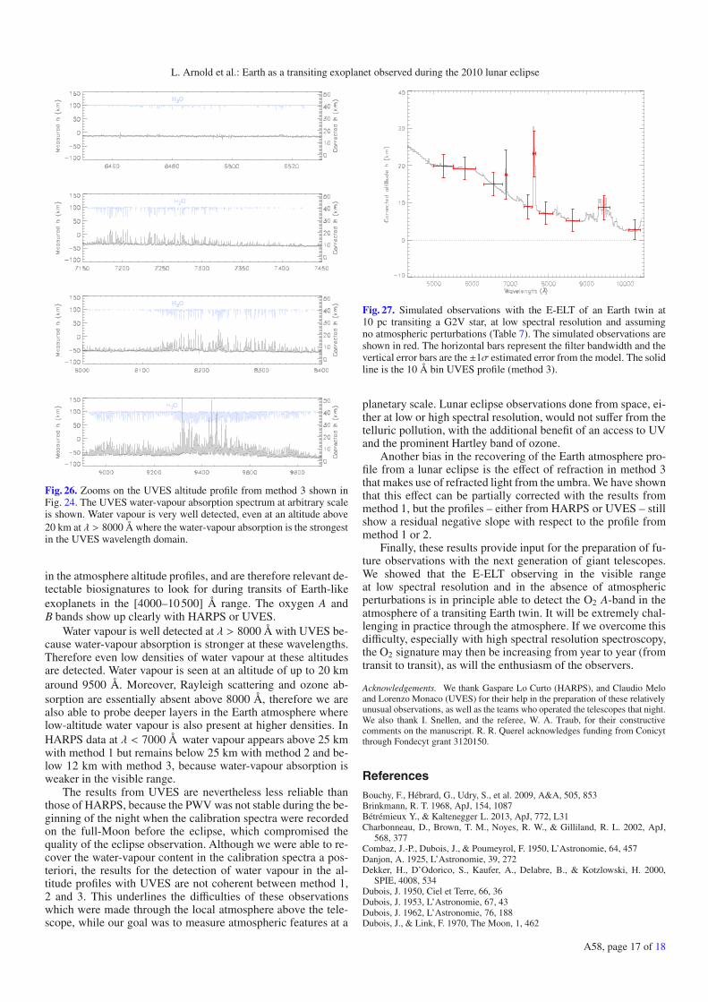