The Effect of Candidate List Position on Vote Share:Improving Internal and External Validity ∗

Kentaro Fukumoto†

Class of 2018, Fast Track Course ‡

January 4, 2018

Abstract

When a candidate is located at a good position (e.g., at the top) on the ballot,the candidate tends to garner larger vote share. It is not, however, straight-forwardto identify position effects unless positions are determined exogenously. An electionto Japanese House of Councilors offers an ideal setup because candidate positons arerandomized across municipalities. Nonetheless, the stable unit treatment value as-sumption does not hold. Accoringly, this paper proposes a new estimand and a newstandard error under a relaxed assumption. We also show that a few estimators havenice properties. Our analysis implies position effects such as the primacy and recencyeffects. We also show that these effects are stronger for non-viable candidates than forviable ones.

∗Paper prepared for delivery at the 1st Annual Meeting of the Japanese Society forQuantitative Political Science, University of Tokyo, January 8–9, 2018, and the 5th AsianPolitical Methodology Meeting, Seoul National University, January 11–12, 2018. Earlierversions of this paper were presented at the Annual Meeting of the Japanese Associationof Elecotral Studies, Kagawa University, May 20–21, 2017, and a workshop at HokkaidoUniversity, March 9, 2017. Fukumoto gratefully acknowledges the financial support of theJapan Society for the Promotion of Science (16K13340) and Sakuradakai.†Professor, Department of Political Science, Gakushuin University. Mailing address: 1-5-1

Mejiro, Toshima, Tokyo 171-8588, Japan. Telephone: +81-3-5904-9258. Fax: +81-3-5992-1006. Email address: Kentaro.Fukumoto@gakushuin.ac.jp. Corresponding author.‡Shuhei Fujita, Yuki Hotsumi, Eri Igarashi, Rei Kawasaki, Chihiro Konjiki, Kentaro

Kuramoto, Yuji Miura, Yuri Nakane, Hinako Saito, Motoki Sasaki, Hiroki Sato, Mami Sato,Rena Wada, Yuki Wanibe, Akane Yamaki, and Ryujiro Yorimitsu. Undergraduate students,Department of Political Science, Gakushuin University.

1

INTRODUCTION

Politicians, judges, and scholars have belived that, when a candidate is located at a good

position (e.g., at the top) on the ballot, the candidate tends to garner larger vote share. Theo-

retically, this “primacy effect” is expected because of cognitive costs of voting, confirmation

bias, satisficing, or “up means good” heuristics (Miller and Krosnick, 1998; Tourangeau,

Couper, and Conrad, 2013).1 Some studies argue that the last position is beneficial because

voters remember the last and forget the first (“recency effect”) (Marcinkiewicz, 2014; Miller

and Krosnick, 1998), while others claim that candidates in the middle positions have larger

vote share (Bagley, 1965; Miller and Krosnick, 1998).

Nonetheless, as Darcy and McAllister (1990) and Miller and Krosnick (1998) well summa-

rize the literature, evidences on these position effects are mixed, partly because candidates’

positions are not (well) randomized and, thus, their effects on vote share are estimated with

bias (see also Ho and Imai, 2008). In this sense, the Japanese upper house elections, which

we study here, offer the most ideal design: the order of the candidates’ names are randomized

for every municipality in a district, which is effectively stratified randomization (Imbens and

Rubin, 2015).

We also argue that, in the previous studies, the stable unit treatment value assumption

(Imbens and Rubin, 2015) (SUTVA) is not plausible and, accordingly, the estimand is not

well defined. This paper proposes a new estimand by relaxing SUTVA. Moreover, we show

that, under stratified randomization, differences-in-means and fixed effects estimators have

nice proporties for this estimand. We also simplfy variance of the differences-in-means esti-

mator and invent the corresponding variance estimator. In these ways, we intend to improve

1 Meredith and Salant (2013) provide evidences which doubt satisficing as a cause of

name position effect. An eye-tracking experiment (Blom-Hansen et al., 2016, 176) discovers

“almost no systematic reading from top to bottom or from left to right.” Thus, they suggest

that “the most likely process behind order effects is spatial [rather than temporal].”

2

internal validity of identifying position effects.

This paper also aims to improve external validity of position effects analysis. As we detail

later, the Japanese setup is not only different from the other countries’ but also, theoretically,

makes it both easy and hard for position effects to work and, thus, be detected. Our findings

of position effects add a new evidence on the debate. We also discover that minor candidates

enjoy stronger position effects than major ones, which is a controversial topic.

The composition of this paper is as follows. The next section elaborates on how we

improve internal and external validity. In the following section, we introduce a new estimand,

estimators, and their variance estimators and show their properties. The fourth section

applies our framework to a dataset of Japan. Finally, we conclude.

GOAL

Internal Validity

In many countries, candidates’ names are placed in the alphabetical order (mostly in British

ex-colonies), in the way a party nominates (mostly under PR system), in the decreasing

order of vote share in a past election, in the order for candidates to file, by incumbency

status, or whether candidates belong to major parites (e.g., Krosnick, Miller, and Tichy,

2004, Table 4.1). In these cases, since there are probably confounders, we cannot be sure of

identifying position effects without bias even with many covariates controlled.

Recently, many studies exploit two types of variation in name order as natural experi-

ments. One is rotation. For instance, in a dozen of American states, the order of candidates’

names is rotated across sub-district areas such as precincts so that one candidate comes at

the top almost as frequently as any other (Krosnick, Miller, and Tichy, 2004, 53). How-

ever, since rotation is conducted in a deterministic way, rotation “is clearly not the same

as random assignment” (Miller and Krosnick, 1998, 299).2 Thus, there might still remain

2 When the name order is rotated from ballots to ballot, it is almost the same as ballot

3

confounders even after controlling pretreatments.

The other way to change the name order is randomization. For example, in Australia,

the order of candidates’ names is randomized for each district (King and Leigh, 2009). Since

the candidates’ names are printed on the ballot in the same order for all voters in the district

unlike rotation, and pretreatments can be unblanced by chance, analysits have to control

candidate’s characteristics in order to improve efficiency of estimation and avoid potential

bias. In particular, when they include candidate fixed effects in panel data, they end up

with only those candidates who run more than once, which might result into selection bias.

Both rotation and randomization are used in California. For every even number year,

a new order of the 26 alphabets is randomly drawn and candidates’ names are reordered

accordingly in a sub-district area. Then, in the other sub-district areas, the order of can-

didates’ names is rotated subsequently. A similar procedure is employed in South Korea

as well (Jun and Min, 2017). These randomization-rotation procedures enjoy best of both

worlds, though analysts can estimate candidate specific effects alone but not average treat-

ment effect and must make much effort to obtain standard errors (Ho and Imai, 2006, 2008)

(these shortcomings hold for non-randomized rotation as well). Moreover, “[w]ith a single

randomization for a single major candidate, ballot order can be highly confounded with

observed and unobserved district characteristics” (Ho and Imai, 2008, 227) (this pitfall is

applied to non-rotated randomization as well).

As Ho and Imai (2008, 227–228) recommend, “[i]f the order were randomized in each

[Assembly] district [for the statewide election], the correlation between ballot order and

. . . any . . . covariate should be zero” (emphasis original). This most ideal setup is exactly

what we study: (not single but) repeated randomization. That is, in the Japanese upper

house elections, the order of the candidates’ names are randomized for every municipality in

level randomization (Darcy 1986, 648, Krosnick, Miller, and Tichy 2004, 53, Orr 2002, 577).

However, we cannot observe for whom each voter casts which type of ballot.

4

the district.3 Therefore, we improve internal validity of analysis to identify position effects.

External Validity

The case of Japan extends the reach of the literature in three directions. First, we examine

the candidate position not on the ballot but on the list displayed at the voting booth. To

our knowledge, all of the previous studies focus on the candidate name order on the ballot.

In Japan, voters write in a candidate’s name on a blank ballot. Instead, at the voting booth,

candidates’ names are displayed on the list.4

Second, we expect and find the primacy effect for the candidate at the top right corner,

not left. This is because, in some situation including candidate lists, Japanese read and

write vertically from right columns to left columns. Our case exemplifies that where is prime

depends on culture.

Third, we document existence of position effects under the single non-transferable vote

(SNTV) system for the first time. Prior research have found the position effect under the

electoral systems of single member districts,5 single transferable votes,6 multiple votes,7 and

open or flexible list proportional representation (PR).8 These three ways, we improve external

3 Public Officers Election Act, Article 175.

4 Public Officers Election Act, Article 175.

5 U.S. and U.K. (Bagley, 1965).

6 Australia (King and Leigh, 2009), Ireland (Robson and Walsh, 1974), Malta, and

U.K. (Curtice and Marsh, 2008).

7 Block vote in the U.S. (Meredith and Salant, 2013), cumulative voting in the

U.S. (Brockington, 2003) and Germany (Marcinkiewicz and Jankowski, 2014), and limited

vote in Spain (Lijphart and Pintor, 1988). Note that some of these works study not national

but local elections.

8 Belgium (van Erkel and Thijssen, 2016; Geys and Heyndels, 2003), Czech (Marcinkiewicz

and Stegmaier, 2015), Denmark (Blom-Hansen et al., 2016), Finland (Ortega Villodres,

5

validity of the position effect research.

We also call attention to the fact that the setup of the Japanese upper house election

makes it both easy and hard for position effects to work and, thus, be detected. To begin,

we look at facilitators. Under the SNTV system, intra-party competetion weakens party

cue and strengthens position effects (cf. Alvarez, Sinclair, and Hasen, 2006; Ho and Imai,

2008; Miller and Krosnick, 1998; Pasek et al., 2014). In addition, the SNTV system has

multiple member districts and, thus, tend to have larger number of candidates. In turn, the

more candidates, the more cognitive cost voters must pay and, thus, the more likely position

effects are to work (Brockington, 2003; Ho and Imai, 2008; Meredith and Salant, 2013).

Nonetheless, there are hurdles as well. Since the election we study is national and,

thus, salient and since party affiliation is shown, voters are given much information about

candidates as well as partisan cues and thus, do not have to rely on candidate positon as

heuristic. In addition, since voting is not compulsory, politically unsofisticated citizens, who

are susceptible to position effects (Miller and Krosnick, 1998; Ho and Imai, 2008), are less

likely to show up.

METHOD

Setup

We index individual canididate and jurisdiction by i and j and their numbers by n and m,

respectively; i ∈ {1, 2, . . . , n}, j ∈ {1, 2, . . . ,m}. Jurisdiction j assigns position indices from

one to n to n candidates without replacement. We denote the position of candidate i in

2003), Germany (Faas and Schoen, 2006), Poland (Marcinkiewicz, 2014), and Switzerland

(Lutz, 2010).

6

jurisdiction j (hereafter, unit ij) by Xij. It follows

X·j ≡ (X1j, X2j, . . . , Xnj)

∈ X

≡{

(x1·, x2·, . . . , xn·)∣∣∣∀x ∈ {1, 2, . . . , n}, n∑

i=1

I(xi· = x) = 1}

where I(·) is a dummy variable to indicate whether the argument is true.

Generally, a treatment variable Wij is a dummy variable dependent on Xij;

Wij = w(Xij) ∈ {0, 1}

For instance, the primacy treatment is defined by W(1)ij where W

(x)ij = I(Xij = x). Denote

the numbers of treated and control units by

n∑i=1

Wij ≡ nT ∈ {0, 1, . . . , n}

n∑i=1

(1−Wij) ≡ nC = n− nT ,

respectively. In particular, when Wij = W(x)ij , x ∈ {1, 2, . . . , n}, it follows that nT = 1.

Denote the (logged or not logged) vote share of unit ij by Yij.

Estimand

Importantly, the two components of the SUTVA are not plausible in our setup. First, the

SUTVA would posit that, for every treatment vector w ≡ (w·1,w·2, . . . ,w·m), there is only

one value of potential outcome, yij(w). This is, however, unlikely to be true in our context.

For instance, Yij tends to be larger when Xij = 2 than when Xij = n (in both cases,

W(1)ij = 0) if the earlier order tends to give a candidate the larger vote share. Instead, we

make the following assumption:

7

Assumption 1 (Single Value). For every assignment vector x ≡ (x·1,x·2, . . . ,x·m), there

is only one value of potential outcome, yij(x).

Second, the SUTVA would require that the potential outcome of Yij is independent of the

other candidates’ positions: yij(x) = yij(x′) if xij = x′ij. This is not, however, plausible in

our setup. For instance, suppose candidates i and i′ belong to the same party, but candidate

i′′ belongs to another party. Then, Yij will be smaller when W(1)i′j = 1,W

(1)i′′j = 0 than when

W(1)i′j = 0,W

(1)i′′j = 1 (in both cases, W

(1)ij = 0) if candidate i′ is more likely to take away

supporters of the same party from candidate i than candidate i′′ is. Instead, we make the

following assumption:

Assumption 2 (No Interference). The potential outcome of Yij is independent of the can-

didates’ positions in the other jurisdictions:

yij(x) = yij(x′) if x·j = x′·j.

This assumption is reasonable because voters do not see candidate lists in the other

jurisdictions.

Hereafter, we denote the potential outcome by yij(x·j), not by yij(wij) ∈ {yij(0), yij(1)}

as under the SUTVA. Note that we cannot define a treatment effect by yij(1) − yij(0).

Instead, to begin, we define the marginal potential outcomes by

yTij ≡1

|XTi· |

∑x·j∈XT

i·

yij(x·j)

yCij ≡1

|XCi· |

∑x·j∈XC

i·

yij(x·j),

where

XTi· ≡ {x·j|Wij = 1,x·j ∈ X}

XCi· ≡ {x·j|Wij = 0,x·j ∈ X}.

8

Then, we define the marginal treatment effect for unit ij by

τMTEij ≡ yTij − yCij

and the average marginal treatment effect (AMTE) by

τAMTE ≡ 1

mn

m∑j=1

n∑i=1

τMTEij .

We denote the super-population average marginal treatment effect by τAMTEsp .

Estimator

Now we presuppose stratified randomization (Imbens and Rubin, 2015), namely, that each

jurisdiction randomly assigns its position vector independently of each other:

Pr(X = x ∈ Xm) =m∏j=1

Pr(X·j = x·j ∈ X) =( 1

|X|

)m=

1

n!m, (1)

where

Xm ≡ {x|∀j ∈ {1, 2, . . . ,m},x·j ∈ X}.

Differnce-in-Means Estimator. We denote the difference-in-means estimator by

τdif ≡ 1

mnT

m∑j=1

n∑i=1

WijYij −1

mnC

m∑j=1

n∑i=1

(1−Wij)Yij.

Generally, it is not guaranteed that τdif is unbiased for the average treatment effect under

stratified randomization (Imbens and Rubin, 2015, 201). Nonetheless, in our design, since

the numbers of treated and control candidates are equal to nT and nC in all jurisdictions,

respectively, the following proposition holds:

9

Proposition 1 (Unbiasedness).

E(τ dif) = τAMTE.

Note that E(·) is expectation operator with respect to X. Proof of all propositions will

be available in to-be appendix.

By contrast, variance estimator for τdif is not straight-forward. The variance of τdif is

derived as

V(τdif) =1

m2

m∑j=1

(STjnT

+SCjnC−STCjn

),

where

STj ≡1

nTV( n∑i=1

WijYij

)SCj ≡

1

nCV( n∑i=1

(1−Wij)Yij

)STCj ≡ 2n

nTnCV( n∑i=1

WijYij,n∑i=1

(1−Wij)Yij

)

and V(·) is variance operator with respect to X. Neyman variance estimator for τdif under

stratified randomization is (Imbens and Rubin, 2015, 202)

VNeyman(τdif) ≡ 1

m2

m∑j=1

( STjnT

+SCjnC

),

where STj and SCj are the sample variance of treated and control candidates within jurisdic-

tion j, respectively:

STj ≡1

nT − 1

n∑i=1

Wij

(Yij −

1

nT

n∑i′=1

Wi′jYi′j

)2SCj ≡

1

nC − 1

n∑i=1

(1−Wij)(Yij −

1

nC

n∑i′=1

(1−Wi′j)Yi′j

)2.

In general, a problem of VNeyman(τdif) is its failure to estimate covariance between treated

10

and control values in a jurisdiction, STCj < 0, due to “the fundamental problem of causal in-

ference.” In addition, in our setup, VNeyman(τdif) does not take into consideration covariance

among treated (or control) values in a jurisdiction because of ignorance to interference be-

tween candidates: V(Yij, Yi′j|Wij = Wi′j = w), w ∈ {0, 1}. Since they can be either positive

or negative, we do not know the direction of bias of VNeyman(τdif). Furthermore, in practice,

when nT = 1, we can calculate neither STj nor VNeyman(τdif) anyway.

Note that, when Y is not-logged vote share,

n∑i=1

Yij = 1.

Therefore,

τdif =n

nC1

mnT

m∑j=1

n∑i=1

WijYij −1

nC

∴ V(τdif) =( n

nC

)2 ST

mnT,

where

ST ≡ 1

m

m∑j=1

STj .

In a nutshell, we only have to care about variation in treated values. In particular, when

nT = 1,

STj =1

n

n∑i=1

(yTij −

1

n

n∑i′=1

yTi′j

)2︸ ︷︷ ︸

variance of mean

+1

n

n∑i=1

E{(Yij − yTij)2|Wij = 1}︸ ︷︷ ︸mean of variance

.

Thus, when Y is not-logged vote share and nT = 1, we propose between variance esti-

mator:

VB(τdif) =( n

n− 1

)2 STm,

11

where adjusted sample variance of treated candidates between jurisdictions is estimated by

ST ≡ 1

N (1) − 1

n∑i=1

(yTi· −

1

N (1)

n∑i′=1

yTi′·

)2︸ ︷︷ ︸

variance of mean

+1

N (2)

n∑i=1

1

Mi − 1

m∑j=1

Wij(Yij − yTi· )2︸ ︷︷ ︸mean of variance

,

the average marginal treated potential outcome of candidate i is estimated by

yTi· ≡1

Mi

m∑j=1

WijYij if Mi ≥ 1,

and Mi ≡∑m

j=1Wij, N(d) ≡

∑ni=1 I(Mi ≥ d).

VB(τdif) solves the problems of VNeyman(τdif); it suffers from failure to estimate neither

STCj nor V(Yij, Yi′j|Wij = Wi′j = w), w ∈ {0, 1}. Above all, we can calculate VB(τdif) even

when nT = 1.

When Y is logged vote share and nT = 1, we regress Y on W alone and calculate the

cluster robust standard error of W ’s coefficient where the cluster is jurisdiction j:

(τ ols, αols) ≡ arg minτols,α

m∑j=1

n∑i=1

(εolsij )2,

where

Yij = α + τ olsWij + εolsij .

Note that τ ols = τdif (Imbens and Rubin, 2015, 118). We use t-distribution, where the degree

of freedom is equal to m.

Fixed Effects Estimator. Difference in vote shares among candidates will be substantial.

For instance, major party candidates tend to obtain larger vote share than minor party

candidates. Thus, we may control candidate fixed effects:

Yij = τFEWij +n∑

i′=1

βi′I(i = i′) +m−1∑j′=1

γj′I(j = j′) + εFEij . (2)

12

As a result, we effectively control usual covariates which affect vote share (e.g. party affilia-

tion, incumbency, seniority, and age). We also control jurisdiction fixed effects. Define the

fixed effects estimator as

(τFE, βFE, γFE) ≡ arg minτFE,β,γ

m∑j=1

n∑i=1

(εFEij )2.

It turns out that, though τFE is not necessarily unbiased for τAMTE in a finite sample any

more (Imbens and Rubin, 2015, Theorem 9.1), the following proposition holds under standard

regularity conditions:9

Proposition 2 (Consistency). τFE is consistent for τAMTEsp .

When Y is not-logged vote share, it holds γj = 0; thus we do not include jurisdiction

fixed effects in Equation 2.

Since Yij’s are dependent on each other within a jurisdiction, we report cluster robust

standard error (where the cluster is jurisdiction j).10 τFE is more efficient than τdif thanks

to candidate fixed effects.

ANALYSIS

Data

We analyze the election to the House of Councillors in Japan held on July 10, 2016. The

election consisted of the national PR tier and the local tier.11 In the latter, each of 47

9 This is because the numbers of treated or control candidates are constant across jurisdic-

tions (nT and nC , respectively). For the same reason, we do not have to include interaction

terms between Wij and I(j = j′)’s so as to obtain a consistent estimator (cf. Imbens and

Rubin, 2015, Theorem 9.2). Note that these hold even if Equation 2 is misspecified.

10 Instead, we may employ blocked bootstrap, where the block is jurisdiction j.

11 Unlike the House of Representatives, there is no link betweeen the two tiers.

13

参議院（東京都選出）議員選挙候補者氏名等掲示

稲城市選挙管理委員会

党とう

派は

名めい

氏し　　　　

名めい

党とう

派は

名めい

氏し　　　　

名めい

日にっ

本ぽん

のこころを

大たい

切せつ

にする党と

う

鈴すず

木き

まりこ国こ

く

民みん

怒いか

りの声こ

え

小こ

林ばやし

こうき

おおさか

維い

新しん

の会か

い

田た

中なか

康やす

夫お

無む

所しょ

属ぞく

原はら

田だ

きみあき

日に

本ほん

共きょう

産さん

党とう

山やま

添ぞえ

拓たく

無む

所しょ

属ぞく

いわさかゆきお

無む

所しょ

属ぞく

三み

宅やけ

洋よう

平へい

公こう

明めい

党とう

竹たけ

谷や

とし子こ

支し

持じ

政せい

党とう

な

し

さめじま良り

ょう

司じ

無む

所しょ

属ぞく

浜はま

田だ

かずゆき

民みん

進しん

党とう

蓮れん

舫ほう

維い

新しん

政せい

党とう

・

新しん

風ぷう

鈴すず

木き

信のぶ

行ゆき

無む

所しょ

属ぞく

よこぼり喜よ

し

久ひさ

無む

所しょ

属ぞく

よこくめ勝か

つ

仁ひと

社しゃ

会かい

民みん

主しゅ

党とう

増ます

山やま

れ

なチャレンジド

日にっ

本ぽん

ふじしろ洋ひ

ろ

行ゆき

支し

持じ

政せい

党とう

な

し

おおつき文ふ

み

彦ひこ

支し

持じ

政せい

党とう

な

し

佐さ

藤とう

ひとし

支し

持じ

政せい

党とう

な

し

深ふか

江え

孝たかし

新しん

党とう

改かい

革かく

たかぎさや

地ち

球きゅう

平へい

和わ

党とう

ひめじけんじ無む

所しょ

属ぞく

鈴すず

木き

たつお

無む

所しょ

属ぞく

柳やなぎ

沢さわ

秀ひで

敏とし

無む

所しょ

属ぞく

佐さ

藤とう

かおり

犬いぬ

丸まる

勝かつ

子こ

と

共きょう

和わ

党とう

犬いぬ

丸まる

勝かつ

子こ

世せ

界かい

経けい

済ざい

共きょう

同どう

体たい

党とう

マタヨシ光み

つ

雄お

民みん

進しん

党とう

小お

川がわ

敏とし

夫お

自じ

由ゆう

民みん

主しゅ

党とう

朝あさ

日ひ

けんたろう

自じ

由ゆう

民みん

主しゅ

党とう

中なか

川がわ

まさはる無む

所しょ

属ぞく

川かわ

上かみ

晃こう

司じ

幸こう

福ふく

実じつ

現げん

党とう

ト

ク

マ

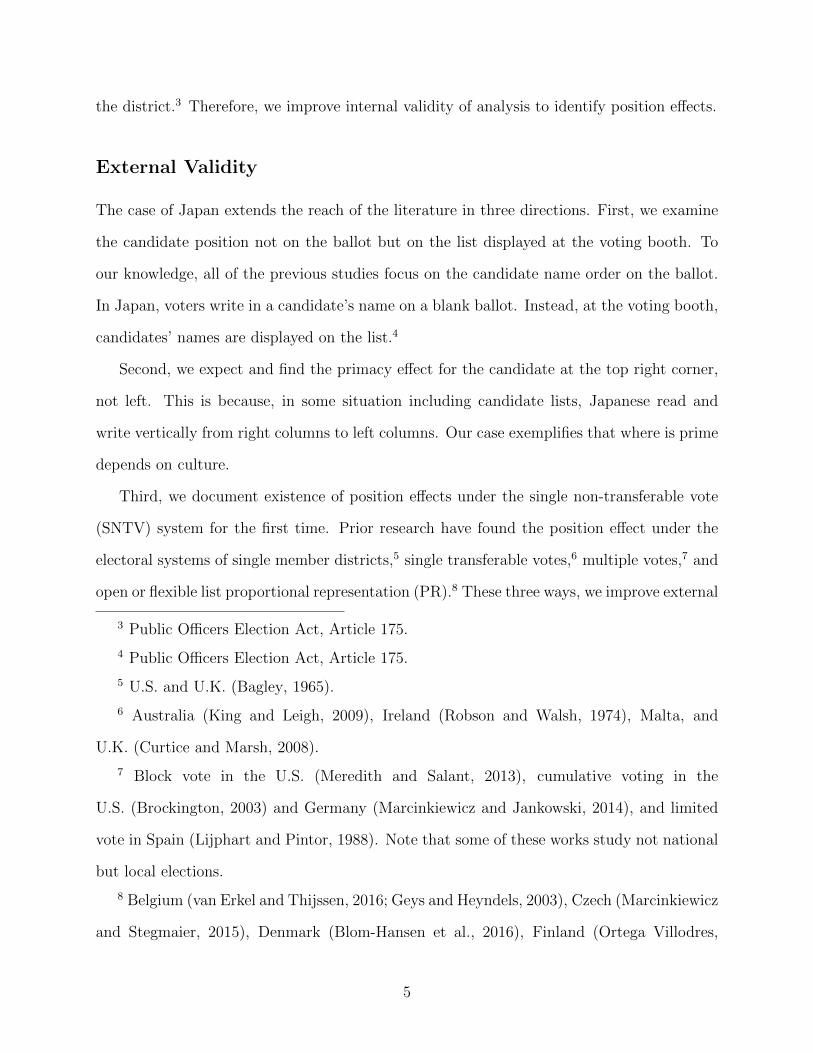
FIGURE 1: The Candidate List in Inagi City.

prefectures composes a SNTV district, where every voter casts a ballot for a candidate.

We study Tokyo prefecure district, which had the most (six) seats and the most (n = 31)

candidates among prefecure districts. In the district, no other election was held on the same

day in any municipality.12

We collect candidate lists at the voting booth from all of 62 municipalities in Tokyo,

sometimes by way of its freedom of information ordinance. An example of the list (Inagi

City) is displayed in Figure 1. The list is displayed in row-horizontal format. The list have

one row in seven municipalities, two rows in 51 municipalities (including Inagi City), and

three rows in four municipalities. Since the position effects will vary across the numbers of

rows, this study focuses on two row lists (thus, m = 51).13

A candidate’s party and name are shown vertically within each cell, though candidates

12 http://www.senkyo.metro.tokyo.jp/election/schedule/senkyo2016/ (access De-

cember 13, 2017).

13 The results for one- or three-row lists will be demonstrated in to-be appendix.

14

are not sorted by party as in the PR tier. Candidates’ occupation, including incumbency

status, race, ethnicity, and gender are not indicated. We refer to each position (or cell) by

row r and column c or, simply, (r, c). In the cases of the top and bottom rows, r = 1 and

r = 2, respectively. Two-row lists have 16 columns. Since Japanese count and read the

vertical format from right columns to left columns, c = 1 and c = 16 in the cases of the most

right and left columns in the top row, respectively. Note that cell (2, 16) is empty.

The board of election in each municipality assigns candidates’ positions by lots inde-

pendently of each other. Thus, we suppose that candidate i in municipality j is placed in

position (Rij, Cij) where

Rij ≡ r(Xij) ≡ 1 + I{Xij > 16}

Cij ≡ c(Xij) ≡ Xij − I(Xij > 16)× 16.

In order to examine not only the primacy and recency effects but also effects of all positions,

this paper focuses on n treatments of position (r, c)’s:

W(r,c)ij ≡ I(Rij = r, Cij = c).

We denote the corresponding AMTE by τ (r,c). For instance, the primacy effect is τ (1,1). Note

that, for all treatmetns, it always holds that nT = 1.14

The dependent variable is either vote share (percentage, 0 ≤ Y not logij ≤ 100) or logarithm

of vote share (Y logij ≤ 0).15

14 In the elections of Brussel Regional Parliament, 75 candidates are displayed in one,

four, or five colomns. Geys and Heyndels (2003) anaylze the effect of top or last position in

each column.

15 The data source is http://www.senkyo.metro.tokyo.jp/election/sanngiin-all/

sanngiin-sokuhou2016/ (access December 13, 2017). The details and descriptive statistics

of the dependent variables are displayed in to-be appendix.

15

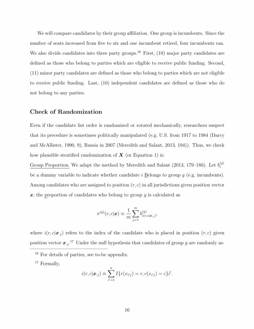
We will compare candidates by their group affiliation. One group is incumbents. Since the

number of seats increased from five to six and one incumbent retired, four incumbents ran.

We also divide candidates into three party groups.16 First, (10) major party candidates are

defined as those who belong to parties which are eligible to receive public funding. Second,

(11) minor party candidates are defined as those who belong to parties which are not eligible

to receive public funding. Last, (10) independent candidates are defined as those who do

not belong to any parties.

Check of Randomization

Even if the candidate list order is randomized or rotated mechanically, researchers suspect

that its precedure is sometimes politically manipulated (e.g. U.S. from 1917 to 1984 (Darcy

and McAllister, 1990, 9), Russia in 2007 (Meredith and Salant, 2013, 194)). Thus, we check

how plausible stratified randomization of X (or Equation 1) is.

Group Proportion. We adapt the method by Meredith and Salant (2013, 179–180). Let b(g)i

be a dummy variable to indicate whether candidate i Belongs to group g (e.g. incumbents).

Among candidates who are assigned to position (r, c) in all jurisdictions given position vector

x, the proportion of candidates who belong to group g is calculated as

π(g)(r, c|x) ≡ 1

m

m∑j=1

b(g)i(r,c|x·j),

where i(r, c|x·j) refers to the index of the candidate who is placed in position (r, c) given

position vector x·j.17 Under the null hypothesis that candidates of group g are randomly as-

16 For details of parties, see to-be appendix.

17 Formally,

i(r, c|x·j) ≡n∑

i′=1

I{r(xi′j) = r, c(xi′j) = c}i′.

16

signed to position (r, c), thanks to the Central Limit Theorem, the distribution of π(g)(r, c|X)

should be approximated by the normal distribution whose mean and standard deviation are

µ(g) ≡ 1

n

n∑i=1

b(g)i , σ(g) ≡

√µ(g)(1− µ(g))

m,

respectively. Let xobs denote the observed value of X. When π(g)(r, c|xobs) does not fall in

the 95% interval of the above normal distribution, we reject the null hypothesis for position

(r, c) at the five percentage significance level.

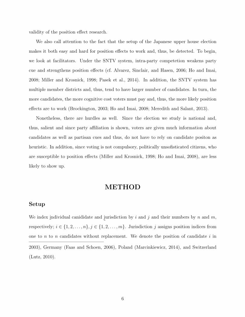
Figure 2 shows results where groups (g) are incumbents (top left), major party (top right),

minor party (bottom left), and incumbent candidates (bottom right). In each panel, the hori-

zonal axis indicates column c, the vertical axis represents group proportion π(g)(r, c|X). The

thick and thin solid lines show π(g)(1, c|xobs) and π(g)(2, c|xobs), respectively. The top, mid-

dle, and bottom horizontal dotted lines correspond to µ(g)+1.96σ(g), µ(g), and µ(g)−1.96σ(g),

respectively. We find that four of 124 (=n positions × 4 groups) or 3.2% of π(g)(r, c|xobs)’s

are outside of the 95% interval (between the top and bottom dotted lines), which is not

surprising under the null hypothesis.

We also test the joint null hypothesis that candidates of group g are randomly assigned

across all positions. We define the group proportion test statistic as the average absolute

value of the difference between π(g)(r, c|X) and µ(g) in each position (r, c):

θ(g)(X) ≡ 1

n

n∑x=1

|π(g){r(x), c(x)|X} − µ(g)|.

The first column of Table 1 displays θ(g)(xobs) for the four groups (in the first through

fourth rows). Analytically, under the joint null hypothesis, the distribution of θ(g)(X) can

be calculated exactly by employing Equation 1. Computationally, however, since we have to

consider all elements of Xm, namely, |Xm| = n!m ≈ 4.6×101729 sets of m lists of n candidates,

it takes extraordinary time. Instead, we approximate the distribution of θ(g)(X) by Monte

Carlo simulation. In the s-th simulation, we randomly draw x(s) from Xm and calculate

17

5 10 15

0.05

0.10

0.15

0.20

Incumbent

Column

Pro

port

ion

5 10 15

0.20

0.30

0.40

Major

Column

Pro

port

ion

5 10 15

0.25

0.35

0.45

Minor

Column

Pro

port

ion

5 10 15

0.20

0.30

0.40

0.50

Independent

Column

Pro

port

ion

FIGURE 2: In each panel, the horizonal axis indicates column c, the vertical axis repre-sents group proportion π(g)(r, c|X). The thick and thin solid lines show π(g)(1, c|xobs) andπ(g)(2, c|xobs), respectively. The top, middle, and bottom horizontal dotted lines correspondto µ(g) + 1.96σ(g), µ(g), and µ(g) − 1.96σ(g), respectively.

θ(g)(x(s)). We repeat this simulation s∗ = 10, 000 times. Then, we estimate one-tail p-value,

p(g) ≡ Pr{θ(g)(X) > θ(g)(xobs)}, by

p(g) ≡ 1

s∗

s∗∑s=1

I{θ(g)(x(s)) > θ(g)(xobs)}.

When p(g) < 0.05, we reject the joint null hypothesis at the five percentage significance level.

The second column of Table 1 reports p-values, which imply that we do not have to reject

the joint null hypothesis.

18

TABLE 1: Group Proportion Test StatisticsGroup (g) θ(g)(xobs) p(g)

Incumbent 0.037 0.592Major 0.046 0.759Minor 0.049 0.623Independent 0.056 0.721

Note: The first clumn reports the value of the group proportion test statistics based on theobserved candidate position. The second column shows one-tail p-values which are estimatedby simulation.

Rank. We adapt the method by Ho and Imai (2008, 222–224) with slight modification. We

calculate the “rank” statistics:

θRank(X) =1

n

n∑i=1

1

n− 1

∑i′ 6=i

1

m

∣∣∣ m∑j=1

(Xij −Xi′j)∣∣∣.

We can estimate the p-value in the same way as θ(g). It turns out that θRank(xobs) =

1.647, pRank = 0.133. Again, there is little evidence that stratified randomization fails.

Treatment Effects

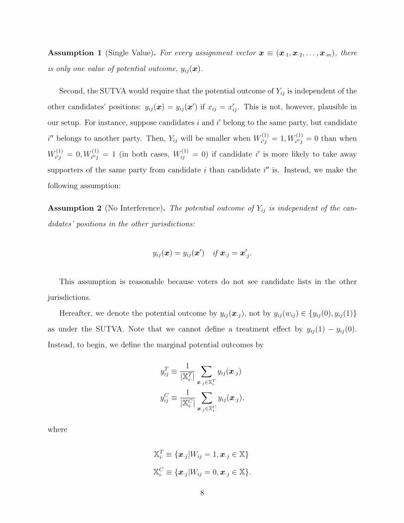
Causal Inference. Figure 3 demonstrate the results of the fixed effect estimator (τFE) where

the dependent variable is the logged vote share (Y log). The left and right panels report the

cases of the top and bottom rows (τ (1,c) and τ (2,c)), respectively. In each panel, the horizonal

axis indicates column (c), while the vertical axis represents exponentiated treatment effects

(exp(τ (r,c))). The thick solid line corresponds to point estimates (exp(τFE(r,c))), while two

thin solid lines represent the upper and lower bounds of the 95 % confidence interval based

on the cluster robust standard error. The horizontal dotted line indicates a reference line of

exp(τ (r,c)) = exp(0) = 1.

In the top row (r = 1, left panel), the primacy effect is significant and substantial:

exp(τFE(1,1)) = 1.520. That is, a candidate in position (1, 1) garners one and half as

19

5 10 15

0.8

1.0

1.2

1.4

1.6

(1) Top Row

Column

exp(

AM

TE

)

5 10 15

0.8

1.0

1.2

1.4

1.6

(2) Bottom Row

Column

exp(

AM

TE

)

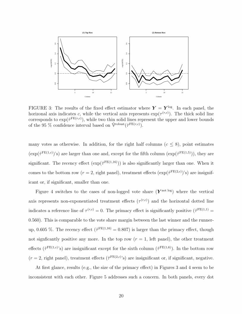
FIGURE 3: The results of the fixed effect estimator where Y = Y log. In each panel, thehorizonal axis indicates c, while the vertical axis represents exp(τ (r,c)). The thick solid linecorresponds to exp(τFE(r,c)), while two thin solid lines represent the upper and lower boundsof the 95 % confidence interval based on Vrobust(τFE(r,c)).

many votes as otherwise. In addition, for the right half columns (c ≤ 8), point estimates

(exp(τFE(1,c))’s) are larger than one and, except for the fifth column (exp(τFE(1,5))), they are

significant. The recency effect (exp(τFE(1,16))) is also significantly larger than one. When it

comes to the bottom row (r = 2, right panel), treatment effects (exp(τFE(2,c))’s) are insignif-

icant or, if significant, smaller than one.

Figure 4 switches to the cases of non-logged vote share (Y not log) where the vertical

axis represents non-exponentiated treatment effects (τ (r,c)) and the horizontal dotted line

indicates a reference line of τ (r,c) = 0. The primacy effect is significantly positive (τFE(1,1) =

0.560). This is comparable to the vote share margin between the last winner and the runner-

up, 0.605 %. The recency effect (τFE(1,16) = 0.807) is larger than the primacy effect, though

not signficantly positive any more. In the top row (r = 1, left panel), the other treatment

effects (τFE(1,c)’s) are insignificant except for the sixth column (τFE(1,6)). In the bottom row

(r = 2, right panel), treatment effects (τFE(2,c)’s) are insignificant or, if significant, negative.

At first glance, results (e.g., the size of the primacy effect) in Figures 3 and 4 seem to be

inconsistent with each other. Figure 5 addresses such a concern. In both panels, every dot

20

5 10 15

−0.

50.

00.

5

(1) Top Row

Column

AM

TE

5 10 15

−0.

50.

00.

5

(2) Bottom Row

Column

AM

TE

FIGURE 4: The results of the fixed effect estimator where Y = Y not log. In each panel,the horizonal axis indicates c, while the vertical axis represents τ (r,c). The thick solid linecorresponds to τFE(r,c), while two thin solid lines represent the upper and lower bounds ofthe 95 % confidence interval based on Vrobust(τFE(r,c)).

represents each candidate, while the vertical and horizontal axes indicate each candidate’s

average vote shares in the treated and control groups (yT (1,1)i· and y

C(1,1)i· ), respectively, where

the treament variable is W (1,1) and 18

yC(1,1)i· ≡ 1

m−M (1,1)i

m∑j=1

(1−W (1,1)ij )Yij if M

(1,1)i ≤ m− 1.

The distance between a dot for candidate i and the 45 degree line is equal to19

τMTE(1,1)i· ≡ y

T (1,1)i· − yC(1,1)

i· .

18 Since N (1)(1,1) = 26 and 0 ≤M(1,1)i ≤ 4 < m− 1, there are 26 dots in each panel.

19 We can interpret τMTE(1,1)i· as a natural estimate of the candidate i’s average MTE:

τMTE(1,1)i· ≡ 1

m

m∑j=1

τMTE(1,1)ij .

21

In the left panel, the dependent variable is the non-logged vote share (Y not log). It turns

out that τMTE(1,1)i· increases in y

T (1,1)i· or y

C(1,1)i· . In the right panel, the dependent variable

is the logged vote share (Y log). Now, τMTE(1,1)i· decreases in y

T (1,1)i· or y

C(1,1)i· . In essence, a

certain percentage points of the primacy effect is relatively large for non-viable candidates

than viable ones.

●●

●

●●●●

●

●●●

●

●●

●

●

●

● ●

●

●

●●

●

●

●

0 5 10 15

05

1015

Vore Share by Candidate (Primacy Treatment)

Average Vore Share in the Control Group (%)

Ave

rage

Vor

e S

hare

in th

e T

reat

ed G

roup

(%

)

●

●

●

●

●

●

●

●

●

●

●

●

●●

●

●

●

● ●

●

●

●

●

●

●

●

−7 −6 −5 −4 −3 −2

−7

−6

−5

−4

−3

−2

Logged Vore Share by Candidate (Primacy Treatment)

Average Logged Vore Share in the Control Group

Ave

rage

Log

ged

Vore

Sha

re in

the

Tre

ated

Gro

up

FIGURE 5: Average vote shares by candidate. Every dot represents each candidate, whilethe vertical and horizontal axes indicate y

T (1,1)i· and y

C(1,1)i· , respectively. In the left and right

panels, the dependent variable is Y not log and Y log, respectively.

In Figures 6 and 7, we apply the difference-in-means estimator τdif to Y log and Y not log,

utilize Vrobust(τdif(r,c)) and VB(τdif(r,c)), and show the results in the same way as in Figures

3 and 4, respectively. Generally, as expected, the standard errors of τdif are larger than

those of τFE. In Figure 6, only exp(τdif(1,1)), exp(τdif(1,2)), and exp(τdif(2,13)) are significantly

different from one (the first two are larger than one, though the last is smaller than one).

In particular, the primacy effect duplicates vote share (exp(τdif(1,1)) = 2.024). In Figure

7, no treatment effect is significantly different from zero, though the primacy and recency

effects are estimated as around one and two percentage points without bias, respectively

(τdif(1,1) = 1.144, τdif(1,16) = 1.800).

Model-based Approach. To sum, we find the primacy and recency effects. Moreover, it seems

that, even if we ignore these two, treatment effects in the top row are larger than those in

22

5 10 15

0.5

1.0

1.5

2.0

2.5

3.0

3.5

(1) Top Row

Column

exp(

AM

TE

)

5 10 15

0.5

1.0

1.5

2.0

2.5

3.0

3.5

(2) Bottom Row

Column

exp(

AM

TE

)

FIGURE 6: The results of the difference-in-means estimator where Y = Y log. In each panel,the horizonal axis indicates c, while the vertical axis represents exp(τ (r,c)). The thick solidline corresponds to exp(τdif(r,c)), while two thin solid lines represent the upper and lowerbounds of the 95 % confidence interval based on Vrobust(τdif(r,c)).

5 10 15

−2

−1

01

23

(1) Top Row

Column

AM

TE

5 10 15

−2

−1

01

23

(2) Bottom Row

Column

AM

TE

FIGURE 7: The results of the difference-in-means estimator where Y = Y not log. In eachpanel, the horizonal axis indicates c, while the vertical axis represents τ (r,c). The thick solidline corresponds to τdif(r,c), while two thin solid lines represent the upper and lower boundsof the 95 % confidence interval based on VB(τdif(r,c)).

the bottom row (τ (1,c) > τ (2,c));20 the treatment effect for a right column is larger than that

20 In the recall election of California Governor in 2003, 135 candidates are carried over

several pages. Ho and Imai (2006) examine the effect of the first page.

23

for a left column in the top row, but not in the bottom row (τ (1,c) > τ (1,c′) if c < c′). In order

to examine these tendencies, we analyze the following regression by OLS:

ylogij = τprimacyI(Rij = 1, Cij = 1) + τ recencyI(Rij = 1, Cij = 16) + τ top rowI(Rij = 1)

+ τ top row × columnI(Rij = 1)× Cij + τbottom row × columnI(Rij = 2)× Cij

+n∑

i′=1

βmodeli′ I(i = i′) +

m∑j′=1

γmodelj′ I(j = j′) + εmodel

ij .

(3)

No coefficients have causal interpretation any more. We use cluster-robust standard error,

where the cluster is jurisdiction (j). According to the first column of Table 2, the result

follows our conjecture; not only τprimacy and τ recency but also τ top row and τ top row × column are

significant, though τbottom row × column is not.

All Incumbent Non-incumbentPrimacy 0.213 ** 0.068 0.240 **

(0.065) (0.059) (0.078)Recency 0.183 ** 0.255 * 0.190 **

(0.056) (0.109) (0.059)Top Row 0.294 ** 0.073 0.316 **

(0.061) (0.057) (0.066)Top Row × Column −0.019 ** −0.014 −0.018 **

(0.005) (0.008) (0.005)Bottom Row × Column 0.000 −0.008 0.001

(0.003) (0.005) (0.003)

N 1581 204 1377

TABLE 2: Results of Model-based Approach

Note: Entries are OLS estimates using Equation 3. Cluster-robust standard error are inparenthesis.

Exploiting benefits of a model-based approach, we divide the dataset by group affiliation

and apply Equation 3 to each sub-dataset so as to study the above empirical regularity

in each group. The second and third columns of Table 2 show the results for incumbents

and non-incumbents, respectively. Clearly, we find the same tendencies for non-incumbents

24

(third column) as for all candidates (first column), but not for incumbents (second column).

In Table 3, candidates are classified into major party, minor party, and independents. All

the coefficients’ sizes for independents (third column) are larger than those for all candidates,

while even τbottom row × column is significant and positive contraty to τ top row × column which is

negative. All the coefficients’ sizes (except for τbottom row × column) for minor party candidates

(second column) are larger than those for major party ones (first column), though τprimacy

and τ recency are insignificant for minor party (for major party, τ top row and τ top row × column are

not significant). Therefore, it seems that candidate positions matter for independents most.

Major Minor IndependentPrimacy 0.157 * 0.218 0.324 **

(0.079) (0.169) (0.103 )Recency 0.162 ** 0.244 0.168 *

(0.060 (0.145) (0.073)Top Row 0.041 0.398 ** 0.451 **

(0.041) (0.094) (0.105)Top Row × Column −0.004 −0.025 ** −0.025 *

(0.005) (0.006) (0.010Bottom Row × Column −0.003 −0.004 0.008 **

(0.003) (0.006) (0.002)

N 510 561 510

TABLE 3: Results of Model-based Approach

Note: Entries are OLS estimates using Equation 3. Cluster-robust standard error are inparenthesis.

These results are consistent with some studies (Meredith and Salant, 2013; Krosnick,

Miller, and Tichy, 2004; Pasek et al., 2014), but not others (Alvarez, Sinclair, and Hasen,

2006; Ho and Imai, 2008; King and Leigh, 2009; Marcinkiewicz and Jankowski, 2014).

25

CONCLUSION

We do not intend to arbitrate the debate on candidate position effects on vote share, while

we hope to add a new evidence for further discussion by improving internal and external

validitity.

On the side of internal validitity, taking into consideration violation of SUTVA, we pro-

pose a new estimand, τAMTE, and a new variance estimator, VB(τdif). We show unbiasedness

of τdif for τAMTE (Proposition 1) and consistency of τFE for τAMTEsp (Proposition 2) under

stratified randomzaition (Equation 1) and Assumptions 1 and 2 which are more relaxed than

SUTVA.

On the side of external validitity, we find the primacy effect (τ (1,1)) and the recency

effect (τ (1,16)) in Japan where candidates’ names are displayed not on the ballot but on the

vertical format list at the voting booth; primacy lies at the top right corner instead of top

left; SNTV is employed. It also turns out that candidates in the top row, in particular

in right columns, tend to obtain more votes. Furthermore, it seems that non-incumbent or

independent candidates are likely to be affected by position effects. We believe accumulation

of findings in various settings improve the literature.

A practical policy suggestion implied by this study is to randomize the list order not

across municipalities as currently implemented but across precincts or even voting booths.

For instance, Setagaya ward has over 749 thousands eligible voters, while Aogashima village

(in Aogashima island) has just 140.21 Benefit of the primacy effect should be more than five

thousands times as large in the former as in the latter. Note that printing various lists is

much less costly than printing various ballots. Our proposal for candidates list should not

add to confusion in counting write-in ballots, either.

Finally, we hope that our study moves forward the research on position effects.

21 http://www.senkyo.metro.tokyo.jp/election/sanngiin-all/

sanngiin-sokuhou2016/ (last access on December 13, 2017).

26

References

Alvarez, R. Michael, Betsy Sinclair, and Richard L. Hasen. 2006. “How Much Is Enough?

The Ballot Order Effect and the Use of Social Science Research in Election Law Disputes.”

Election Law Journal 5(1): 40–56.

Bagley, C R. 1965. “Does Candidates’ Position On The Ballot Paper Influence Voters’

Choice? – A Study Of The 1959 and 1964 British General Elections.” Parliamentary

Affairs 19(2): 162–174.

Blom-Hansen, Jens, Jørgen Elklit, Søren Serritzlew, and Louise Riis Villadsen. 2016. “Ballot

position and election results: Evidence from a natural experiment.” Electoral Studies

44(dec): 172–183.

Brockington, David. 2003. “A low information theory of ballot position effect.”.

Curtice, John, and Michael Marsh. 2008. “How Did They Vote? Voters’ Use of the STV

Ballot Paper in the 2007 Scottish Local Elections.” Representation 44(4): 285–300.

Darcy, R. 1986. “Position Effects with Party Column Ballots.” The Western Political Quar-

terly 39(4): 648–662.

Darcy, R., and Ian McAllister. 1990. “Ballot position effects.” Electoral Studies 9(mar):

5–17.

Faas, Thorsten, and Harald Schoen. 2006. “The importance of being first: Effects of can-

didates’ list positions in the 2003 Bavarian state election.” Electoral Studies 25(mar):

91–102.

Geys, Benny, and Bruno Heyndels. 2003. “Ballot layout effects in the 1995 elections of the

Brussels’ government.”.

Ho, Daniel E, and Kosuke Imai. 2006. “Randomization Inference With Natural Experi-

ments.” Journal of the American Statistical Association 101(sep): 888–900.

27

Ho, Daniel E., and Kosuke Imai. 2008. “Estimating causal effects of ballot order from a

randomized natural experiment: The California alphabet lottery, 1978-2002.”.

Imbens, Guido W., and Donald B. Rubin. 2015. Causal Inference for Statistics, Social, and

Biomedical Sciences. Cambridge University Press.

Jun, Byung-hill, and Heechul Min. 2017. “What creates heterogeneity in ballot order effects?

Evidence from Korea’s local elections of education superintendent.” Electoral Studies 46:

1–14.

King, Amy, and Andrew Leigh. 2009. “Are ballot order effects heterogeneous?” Social

Science Quarterly 90(1): 71–87.

Krosnick, Jon A., Joanne Miller, and M. P. Tichy. 2004. “An unrecognized need for ballot re-

form: Effects of candidate name order.” In Rethinking the vote: The politics and prospects

of American election reform., ed. A. N. Crigler, M. R. Just, and E. J. McCaffery. New

York, NY:: Oxford University Press.

Lijphart, Arend, and Rafael L?pez Pintor. 1988. “Alphabetic bias in partisan elections:

Patterns of voting for the Spanish Senate, 1982 and 1986.” Electoral Studies 7(dec): 225–

231.

Lutz, Georg. 2010. “First come, first served: The effect of ballot position on electoral success

in open ballot PR elections.” Representation 46(2): 167–181.

Marcinkiewicz, Kamil. 2014. “Electoral contexts that assist voter coordination: Ballot posi-

tion effects in Poland.” Electoral Studies 33: 322–334.

Marcinkiewicz, Kamil, and Mary Stegmaier. 2015. “Ballot Position Effects Under Com-

pulsory and Optional Preferential-List PR Electoral Systems.” Political Behavior 37(2):

465–486.

28

Marcinkiewicz, Kamil, and Michael Jankowski. 2014. “When There’s No Easy Way Out:

Electoral Law Reform and Ballot Position Effects in the 2011 Hamburg State Elections.”

German Politics 23(1-2): 103–117.

Meredith, Marc, and Yuval Salant. 2013. “On the Causes and Consequences of Ballot Order

Effects.” Political Behavior 35(1): 175–197.

Miller, Joanne M, and John Krosnick. 1998. “The Impact of Name Order on Election

Outcomes.” Public Opinion Quarterly 62(3): 291–330.

Orr, Graeme. 2002. “Ballot Order: Donkey Voting in Australia.” Election Law Journal:

Rules, Politics, and Policy 1(dec): 573–578.

Ortega Villodres, Carmen. 2003. “Intraparty Competition Under Preferential List Systems:

The Case of Finland.” Representation 40(1): 55–66.

Pasek, Josh, Daniel Schneider, Jon A. Krosnick, Alexander Tahk, Eyal Ophir, and Claire

Milligan. 2014. “Prevalence and moderators of the candidate name-order effect evidence

from statewide general elections in California.” Public Opinion Quarterly 78(2).

Robson, Christopher, and Brendan Walsh. 1974. “The Importance of Positional Voting Bias

in the Irish General Election of 1973.” Political Studies 22(jun): 191–203.

Tourangeau, Roger, Mick P. Couper, and Frederick G. Conrad. 2013. “Up means good: The

effect of screen position on evaluative ratings in web surveys.”.

van Erkel, Patrick F.A., and Peter Thijssen. 2016. “The first one wins: Distilling the primacy

effect.” Electoral Studies 44(dec): 245–254.

29