The Dynamics of Exchange Rate Regimes: Fixes, Floats, and Flips∗

by

Michael W. Klein Fletcher School, Tufts University and NBER

and

Jay C. Shambaugh+

Dartmouth College and NBER

July 26, 2007

Abstract: The impermanence of fixed exchange rates has become a stylized fact in international finance. The combination of the “mirage” view that pegs do not really peg with the “fear of floating” view that floats do not really float generates the conclusion that exchange rate regimes are, in practice, unimportant for the behavior of the exchange rate. This is consistent with evidence on the irrelevance of exchange rate regimes for general macroeconomic performance. Recent studies, however, show that the exchange rate regime matters. This can be understood by considering the dynamics of exchange rate regimes. We demonstrate that the “mirage” view is somewhat misleading and incomplete. Pegs frequently break, but many do last. Also, there is a high degree of flipping, that is, the re-formation of pegs that have broken. Thus, a fixed exchange rate today is a good predictor that one will exist in the future. We also investigate the quantitative effect of fixed exchange rates. While the “fear of floating” view suggests little actual difference in fixed and floating rates with respect to exchange rate volatility, we show that fixed exchange rates exhibit considerably greater bilateral exchange rate stability than flexible rates, both today and in the future.

JEL Codes: F3, F4

Keywords: Exchange Rate Regimes, Fixed Exchange Rate,

∗ We thank Eric Edmonds, Philip Lane, our discussants Christian Broda and Paolo Mauro, and participants at the NBER IFM program meetings, Exchange Rates: Choices and Consequences Conference at Cambridge University, IIIS Trinity College Dublin, and the Dartmouth International Brown Bag for helpful discussion and Pooneet Kant for research assistance. We also thank the editor, Charles Engel, and two anonymous referees for very helpful suggestions. We also thank Federico Sturzenegger, Carmen Reinhart, and Barry Eichengreen for making their data available on their website. All errors are ours. + Corresponding author: email: Jay.C.Shambaugh@Dartmouth.edu, phone: 603-646-9345, address: HB 6106, Dartmouth College, Hanover NH 03755

1

The choice of an exchange rate regime, and the consequences of this choice, traditionally

represents a central topic in international finance. But, recently, research has called into question the

relevance of this line of inquiry. This is demonstrated by two of the more evocative titles in

international finance articles published in the last decade, “The Mirage of Fixed Exchange Rates”

(Obstfeld and Rogoff 1995), and “The Fear of Floating” (Calvo and Reinhart 2002). Obstfeld and

Rogoff (1995) suggest that fixed rates are not all that fixed, writing “literally only a handful of

countries in the world today have continuously maintained tightly fixed exchange rates against any

currency for five years or more.” [p. 87] Calvo and Reinhart (2002) argue that floating rates do not

really float, rather governments that claim to allow market forces to determine the value of their

currencies actually act to minimize exchange rate fluctuations.

Taken together, these influential articles suggest that the exchange rate regime is, in practice,

unimportant and perhaps irrelevant for the actual behavior of the exchange rate. This conclusion is

bolstered by empirical research that finds little role for exchange rate regimes in determining major

macroeconomic outcomes beyond the real exchange rate (see Mussa 1986, Baxter and Stockman 1989,

and Flood and Rose 1995). Altogether, based on these works, there is a general impression that

exchange rate regimes – in spite of all the attention they receive – are in some ways unimportant.

In this paper we bolster the traditional view of the importance of the exchange rate regime.

One of our central results shows that fixed exchange rates are more substantial than mere mirages;

while almost half of the fixed exchange rate spells do not last more than two years, the expected

duration of a peg increases dramatically if it survives past that age. Consequently, at any one time, the

set of countries that are pegged includes a large proportion of those with a peg lasting for a relatively

long duration. We also show that the distribution of floating exchange rate spells is similar to the

distribution of fixed exchange rate spells, with a large number of short-lived floating exchange rate

spells and a smaller number of long-lived floating exchange rate spells. An important implication of

this is the flipping of pegged rates, that is, the end of a peg is often followed by the re-formation of a

new peg. This dynamic behavior of exchange rate regimes, when combined with an analysis of the

duration of fixed exchange rate spells and floating exchange rate spells, paints a different picture than

one would expect from the well-known “mirage” of fixed exchange rates.

The mere classification of annual observations into those categorized as “pegs” and those

categorized as “floats” (or, more accurately, non-pegs) would not matter if the “fear of floating” truly

limited exchange rate flexibility when countries do not peg. We demonstrate, however, that the

magnitude of bilateral exchange rate volatility between a country that has a pegged rate and its base

2

country is quite distinct from bilateral volatility when a country does not peg.1 Countries that peg have

lower multilateral volatility as well, mainly because these countries tend to avoid extreme bilateral

volatility outcomes.2

Taken together, these two results, on the dynamics of exchange rate regimes and the

implications of the exchange rate regime for volatility, implies that a country with a fixed exchange

rate today can be expected to exhibit greater exchange rate stability both today and over the course of

time. This helps explain some current evidence on the effects of exchange rate regimes, including the

significant and positive effect of fixed exchange rates on trade (Klein and Shambaugh 2006), the limits

that fixed exchange rates place on monetary autonomy (Shambaugh 2004, and Obstfeld, Shambaugh,

and Taylor 2005), and the effects of the exchange rate regime on the transmission of terms of trade

shocks (Broda 2004, and Edwards and Levy-Yeyati 2005), the national price level (Broda

forthcoming) and inflation (Ghosh, Gulde, and Wolf 2002). The results presented in this paper also

help explain why research has found that the exchange rate regime plays a role in determing the rate of

growth (Aghion, Bachetta, Ranciere and Rogoff 2006, Levy-Yeyati and Sturzenegger 2003, Husain et

al. 2005, di Giovanni and Shambaugh 2006, and Ghosh et al. 2002) and growth volatility (Ghosh et al.

1997).

Thus, this paper demonstrates the extent to which exchange rate regimes really do matter for

exchange rate outcomes, and helps explain the source of effects of recent research demonstrating trade

and macroeconomic consequences of exchange rate regimes. It examines the nature of de facto

exchange rate regimes themselves, studying their duration, dynamics, and the extent they affect the

exchange rate. In essence, we try to provide a new set of stylized facts on exchange rate regimes that

helps explain why the new wave of empirical evidence on their effects can occur.

II. Exchange Rate Spells, Fixed and Floating

A central part of this study, or any other one that focuses on the role of the exchange rate

regime, is its definitions of the regimes themselves. It has been well documented that governments’

declarations to the International Monetary Fund as to the exchange rate regimes in place are not always

accurate (see, for example, Calvo and Reinhart 2002). Therefore, in this paper we rely on de facto

1 This is not to argue that no countries manage their nonpegged exchange rates, or that no countries mis-declare their regimes, but to say that some countries actually do float and their exchange rates are notably more volatile than the pegs. 2 As discussed below, implications of these distinct effects between bilateral and multilateral outcomes relate to differences in trade and macroeconomic outcomes since bilateral volatility affects bilateral trade and macroeconomic stability while economic growth, for example, may require a broader effect across many sectors that is more closely associated with multilateral stability.

3

exchange rate behavior rather than de jure declarations of whether a country has a fixed or a flexible

exchange rate.3

The basis of our coding a country as having a fixed or a floating (i.e. not a fixed) exchange rate

is a modification of the classification scheme used by Shambaugh (2004) who, in turn, closely

followed the method employed by Obstfeld and Rogoff (1995).4 In this paper, we considered a

country as having a fixed exchange rate in a given calendar year, with its currency pegged to the

currency of a base country, if its month-end official bilateral exchange rate stays within the same +/-

2% band for the entire year. This requires that a currency is within the same +/- 2% band at the end of

each month for the full year. We do not classify a country as having a pegged exchange rate if the

change in its exchange rate between January and December is less than 2% but its currency moved

outside the +/- 2% band during any month in that year. The coding is annual and, therefore, the peg

must last for a full calendar year for a country to be classified as pegged for that year. Pegs that last

less than a full year are classified as nonpegs.5 An advantage of such a procedure, as opposed to

looking at relative volatility benchmarks is that this definition of a peg (within a 2% band) is clear,

invariant over time, and matches the historical definitions of pegs such as the gold points in the Gold

Standard, the bands in Bretton Woods and the EMS. 6

The base country is determined through the pegging history of a given country as well as

through tests against a variety of countries, the declared intent of the country, and readings of various

3 Our focus is on new stylized facts for de facto regimes. There is another strand of research that explores why de facto activities and de jure declarations can conflict. Alesina and Wagner (2006) investigate why some countries behave more restrictively than they declare or vice verse. Genberg and Swoboda (2005) discuss reasons why a government may peg an exchange rate without declaring that as its goal which suggests that de jure declared regimes may not really represent the true goals or actual intent of a government. 4 Two other prominent studies that developed a classification scheme for exchange rate regimes are Levy-Yeyati and Sturzeneggar (2003) and Reinhart and Rogoff (2004). The classification used by Levy-Yeyati and Sturzenegger (2003) uses information on reserves as well as currency values such that stable rates in the absence of reserve changes might not be called pegs while somewhat volatile exchange rates paired with extensive intervention may be considered as pegged. Reinhart and Rogoff (2004) use parallel market rates and focus on the conditional probability of staying within a range over a five year period, a method that could bias our results to finding long lived pegs. In an appendix we provide detailed analysis of alternate classifications. We compare our classification with these others, as well as the declared status countries report to the IMF, in the body of the text, although the use of the LYS classification for the duration analysis presented below is difficult due to the presence of observations marked “inconclusive” in that coding. 5 For example, a country with a peg lasting from June 2001 to May 2005 would be classified as floating in 2001 and 2005 and pegged from 2002 – 2004. While there may be pegs, or attempted pegs, shorter than one year, our view is that for the time spans less than one year it becomes increasingly likely that the stability one would find in the data is an accident and not a peg – false positives would rise. Also, we posit that market participants will not have detected or believed a peg until it has lasted more than a few months. 6 Results are not sensitive to the defined width of the band. Most of the pegged observations stay within an even tighter band, but 2% is consistent with Obstfeld and Rogoff (1995). 7 observations in the EMS are counted as floats but would stay within a 4.5% range allowed in the EMS’s 2.25% bands (assuming the countries were staying within the bounds, not moving outside them with the 4.5% range). Re-coding these observations makes little difference to any numbers reported.

4

currency histories. For the purpose of comparative bilateral volatility tests, we need a “base” country

for countries when they have a floating exchange rate. In these cases, the base is the country to which

the country with the floating exchange rate pegged in the past, or a major industrial country with which

it has a prominent economic relationships (for details see Shambaugh 2004).7 We drop from our

sample countries with a population of less than 400,000 in 1999. We also drop observations that

represent currency unions (but for the members of the single currency in Europe from 1999 onwards)

in order to keep these episodes from biasing the sample towards long-lasting fixed exchange rate

pegs.8 The United States is not included in the data set.

While one might be concerned that a country / year observation is being classified as a peg

simply due to a lack of shocks, Calvo and Reinhart show that the probability that the bilateral

exchange rate had a monthly change of less than 2.5% was roughly 60-70% during classic floats like

the US dollar / DM rate, the US dollar / yen rate or the US dollar / Australia dollar rate. In these cases,

the probability of 12 straight months of changes smaller than 2.5% (in either direction) is between 0

and 1%. In addition, as stated above, our classification requires the tighter restriction of staying within

the same +/- 2% bands over each successive month of the entire year and for the year as a whole. This

is more restrictive than a condition where the fluctuation from one month to the next month is smaller

than +/- 2% but a currency could drift by more than +/- 2% over the course of a year. Thus, the odds

of “accidentally” coding a peg when, in fact, a currency is floating are extremely low with the

classification scheme that we use. Evidence for this comes from the fact that currencies that are well

known to be floating, such as the Australian dollar or the Japanese yen, are never coded as pegs in our

classification system. 9 Also, the undeclared pegs in our coding, those countries / year observations

that we code as de facto pegs but are not de jure pegs, are typically instances generally recognize as

pegs, such as with the currencies of East Asian countries in the early 1990’s.10

7 There are a limited number of changes in the base country. In these cases, the switch is generally a direct change in the peg (as in the case of some former British colonies that change to a dollar base) so coding the timing of the switch is automatic. In other cases, discretion is used to mark the change in base. 8 Obstfeld and Rogoff (1995) identify 27 small countries with long lasting pegs in their Tables 2 and 3. By dropping countries with small populations, and currency unions, we retain only 8 of these 27; Bahrain, Djibouti, Lesotho, Namibia, Oman, Qatar, Swaziland, and United Arab Emirates. We set the population hurdle at 400,000 in order to retain in our data set the smallest country that Obstfeld and Rogoff keep (Luxembourg) and yet to exclude most of the countries they exclude. 9 Countries not based on the dollar, such as EMS countries or African countries pegged to the Franc, also show roughly a 60% chances of having their exchange rate against the dollar stay within 2.5% bands. This suggest only a 0.2% chance of maintaining a peg, for 12 months in a row, and an even lower chance of being within the same 2% bands over a year. 10 Shambaugh (2004), by requiring two consecutive years of staying in a band to have an observation qualify as a peg, effectively ruled out any coding of unintentional pegs. We do not follow this procedure since dropping single year pegs would bias our results towards finding longer pegs by eliminating short lived pegs. Shambaugh (2004) also considered one-time discrete devaluations (one month with a change in the exchange rate greater than 2%, but 11

5

In the interest of robustness, we consider reclassifying a set of single year pegs that seem most

likely to be unintentional, those that are neither de jure pegs nor are coded as pegged by either

Reinhart and Rogoff (2004) (RR) or by Levy-Yeyati and Sturzenegger (2003) (LYS). There are 39

country / year observations that fit within this category. Within this set, the exchange rate of 12 single

year pegs remained within a +/- 1% band, a situation that is highly unlikely to have arisen accidentally.

Thus, we focus on the 27 “questionable peg” observations that are within 2% bands and are neither

declared nor identified as a peg by RR nor by LYS. This set of observations represents 20 countries

and 16 different years, and, therefore, is not evidence of a lack of world volatility in a particular year

or country. It also includes many country / year observations that are widely considered to be de facto

pegs, such as Malaysia and Indonesia in 1996, as well as countries whose currency was clearly

shadowing that of another country, such as Portugal in 1975 which was linked to the DM unofficially

in the Snake. Other countries, such as India, Pakistan, Tunisia, and Jamaica, all of which have two

“questionable” single year pegs, have many other unquestionable pegs in the sample, making it

unlikely that the “questionable” peg is just an accident of coding. Nevertheless, we repeat our

analysis below coding these 27 observations as nonpegs. We find no change in the volatility results

and only small differences in the duration and dynamics results.11

In this work, we focus on the differences between actually being pegged and not being pegged.

We do not attempt to distinguish among a set of intermediate regimes because this would necessarily

introduce more errors to a classification scheme since the boundary between a de facto peg and a

nonpeg can be fairly clearly draw while the lines separating one intermediate regime from another is

much less distinct. For example, some of the most freely floating countries manage their exchange

rate to some extent, but it is difficult, in practice, to distinguish these managed floats from target zones

with wide and movable bands.

Table 1 presents statistics on the prevalence of fixed and floating exchange rates in our panel

data set that covers the period 1973 - 2004. This first two columns show that this data set is drawn

from the experience of 125 countries, 21 of which we classify as major industrial countries (those that

began the period as members of the OECD). Of the 3,924 country / year observations in this data set,

months exactly equal to zero) as pegs, but here we count these as breaks in the peg to avoid a bias towards finding long lasting pegs and to avoid artificially increasing the length of peg spells by, for example, defining a country as a peg even if it devalues every other year but otherwise stays pegged. As discussed in more detail in the appendix, this treatment of devaluations distinguishes the main coding used here from Reinhart and Rogoff, Shambaugh, and de jure classifications that allow devaluations, making the main coding quite similar to the way Obstfeld and Rogoff scheme. 11 We cannot identify countries that attempted to peg in a particular year but failed. These observations would be coded as floats, which is appropriate for our analysis since we are investigating the characteristics of actual pegs, not the implications of unfulfilled desires.

6

47.53 percent are pegs.12 Pegs are more prevalent among developing countries than among industrial

countries, with 49.22 percent of the developing country / year observations representing pegs but only

39.34 percent of the industrial country / year observations representing pegs.

Table 1 also presents some basic statistics on fixed and floating exchange rate spells. A peg

spell is a set of consecutive years during which a country continually pegs its currency, and a float

spell is a set of consecutive years during which a country continually does not peg its currency. These

spells are the basic unit of analysis in this paper. We focus on spells to understand the extent to which

a particular peg lasts as opposed to over-arching policy regimes. The minimum spell duration is 1

year, and the maximum spell duration is 32 years, the full length of the sample period. The statistics in

Table 1 show that there are 398 peg spells in our panel, with an average of 3.18 peg spells per country,

and 395 float spells, with an average of 3.16 float spells per country. The median duration of both peg

and float spells is 2 years, and the mean durations are also similar, with the average peg spell lasting

for 4.67 years and the average float spell lasting for 5.21 years. There are not dramatic differences in

these statistics between the 21 major industrial countries and the 104 other countries included in the

sample. The differences between the means and the medians of peg and float spells, and the size of the

standard deviations relative to the means for both types of spells, suggest skewness in the distribution.

This is demonstrated in the histograms in Figures 1 and 2 that show that both peg and float spells are

characterized by a large number of spells with very short duration, and a smaller number of spells with

longer duration.13

A motivation for using a coding that requires a continuous, unvarying peg as opposed to one

that allows discrete devaluations in addition to unbroken pegs is that these two types of experiences

are different from the perspective of economic agents. The mean length of both peg spells and float

spells would be longer if one counted a peg spell broken by a one-time devaluation to count as a

continuous peg (as is done with the Reinhart and Rogoff, Shambaugh, or de jure codings) rather than

as two separate pegs with an interceding one-year float spell at the time of the devaluation (as is done

with our main classification scheme).14 This is one source of the difference in statistics on peg and

float spells between our main classification scheme and that of Shambaugh (2004) or of Reinhart and

Rogoff, as shown in the Appendix. 15 In particular, Reinhart and Rogoff smooth regimes over time by

12 There are 3,924 observations, rather than 125 × 32 = 4000, because 76 observations represent currency unions. 13 Klein and Marion (1997) show that exchange rate pegs among Latin American and Caribbean countries are also characterized by a large number of very short pegs and a smaller number of long-lived pegs. 14 Obstfeld and Rogoff (1996) do not count an episode that includes a one-time devaluation as a continuous peg. 15 In his study of inflation targeting in which he uses peg duration as an indicator of monetary regimes, Rose (2006) examines the durability of exchange rate regimes and finds pegs are fragile using a set of countries in the 1990s using both Reinhart and Rogoff and Levy-Yeyati and Sturzenegger coding.

7

relying on exchange rate behavior over five year windows. This allows them to focus on identifying

exchange rate policy over time rather than specific spells, and, accordingly, they find much longer

lived regimes than what we find by considering spells.16 Thus, the classifications are not imperfectly

measuring the same experience, but are often simply trying to identify different things.

The large number of both peg and float spells that have short duration in our data is also

evident from the statistics in Table 2. These statistics show that about 56 percent of the peg spells, and

about 65 percent of the float spells, survive for at least two years; of course, this means that 44 percent

of the peg spells and 36 percent of the float spells last for only one year. Somewhat less than a third of

the peg spells (30.14 percent) and a little more than a third of the float spells (33.97 percent) last for at

least 5 years. While the view that pegs frequently break is not uncommon, the result presented here,

that floats are equally fleeting, is more novel. As seen in the 4th column of table 2, a large number of

broken pegs have repegged by the third year after breaking the peg (only 48% of floats last 3 years).

The view that countries flip back and forth in their exchange rate arrangements differs from the more

simplistic, and less accurate, view that a crisis forces a peg to break and, subsequently, a country floats

permanently thereafter.

The general finding, that over 70% of peg spells do not last over five years, confirms the basic

idea of Obstfeld and Rogoff (1995) that a majority of pegs are short-lived. On the other hand, a fair

number do last long term, more than the “handful” suggested by Obstfeld and Rogoff, and certainly

more than that suggested by the stylized fact that all pegs break. 17 There are two sources of the

difference in our results from those of Obstfeld and Rogoff (1995). One is that we include some

countries omitted by Obstfeld and Rogoff because our strict population cutoff includes some countries

with relatively large populations that Obstfeld and Rogoff considered “small”. The second, more

important, reason for the difference concerns the timing of Obstfeld and Rogoff’s study. Their paper

was, in part, motivated to explain why pegs in the mid-1990s were not lasting, as evidenced by the fact

that many countries in the EMS that could have defended their pegs chose not to do so. This may

have been due to the development of deeper capital markets that made pegging more difficult. The

1995 date of their study meant that many longstanding pegs had ended in the previous few years due to

the EMS crisis, the Tequila Crisis, and the devaluation of the CFA countries against the franc. Despite

the size and speed of capital markets, though, many of these broken pegs were subsequently re-

established and also new pegs were created after 1995, with the result that there were just as many 16 See Husain, Mody, and Rogoff (2005) who give details on regime duration and comment in their footnote 8, “the Natural Classification [RR] attempts to identify longer term regimes rather than short term “spells.” 17 Obstfeld and Rogoff (1995) write “The striking conclusion from Table 2 is that aside from some small tourism economies, oil sheikdoms, and highly dependent principalities, literally only a handful of countries in the world today have maintained tightly fixed exchange rates against any currency for five years or more.” (p. 87, italics in original).

8

long-lived pegs in 2000 as there were in 1990. Figure 3 shows that, in our classification, the period

from 1994-1998 was the low point of long-lived pegs with only an average 17 in those years (out of

roughly 125 countries in the sample)18 as compared to a post Bretton Woods average of 32 long-lived

pegs, and 36 long-lived pegs in 2000.19 Thus, a focus on the entire post–Bretton Woods era, rather

than the situation in 1995, and on peg spells, rather than countries, alters the impression one has of the

durability of exchange rate pegs.20

A country that flips from a peg to a float and back to a peg again might represent an inability to

maintain a consistent exchange rate regime. If this inability to maintain a consistent policy was

pervasive, we would expect to find relatively few instances of long-lived spells. In fact, the statistics

presented in Table 3 shows that this is not the case. This table presents the longest peg duration and

the longest float duration for each of the 125 countries in the sample. Almost 70 % of the countries in

the sample have peg spells of 4 or more years, and 70 % have float spells of 5 or more years. Of

course, we cannot know the intentions of the 12% of countries that either never peg or have no peg

spells that last more than one year, and the 20% of countries that either never float or have no float

spell that lasts for more than one year. It seems unlikely, however, that Israel could not peg for more

than one year (its maximum peg is one year) or Syria could not float for more than one year (its

maximum float is one year). Rather, these outcomes seem to reflect policy choices. Similarly, a

country like Canada has never pegged for more than two years at a time, but certainly other large

industrial countries (e.g. France, who has stayed within its EMS bands every year since 1987) have

been able to do so.

A more complete characterization of these spells involves an analysis of their survival rates,

duration dependence, and factors that affect their duration dependence. We next turn to these issues.

18 The panel is roughly balanced with between 122 and 125 countries in the sample. The slight variation comes from the fact that currency unions are eliminated from sample with the exception of spells that began as pegs and converted to currency unions (e.g. some EMU observations) 19 Pegs lasting at least 5 years in 2000 includes some oil countries and the CFA countries, but also many EU nations as well as Argentina, China, and El Salvador. The full list is: Argentina, Austria, Bahrain, Belgium, Benin, Burkina Faso, Cameroon, Central African Republic, Chad, China, Comoros, Republic of Congo, Cote D’Ivoire, Denmark, Djibouti, El Salvador, Equatorial Guinea, Gabon, Hong Kong, Jordan, Lebanon, Lesotho, Luxembourg, Mali, Namibia, Nepal, Netherlands, Niger, Oman, Qatar, Saudi Arabia, Senegal, Swaziland, Syria, Togo, UAE. 20 As demonstrated by the figures in the Appendix, other classification schemes also show the early nineties as a low in terms of the number of long pegs and all show today as a post Bretton Woods high. Given that the other classifications allow a discrete devaluation, they do not show a large drop in the number of 5 year pegs after the EMS and CFA crises, but the overall message is the same.

9

III. Exchange Rate Spells: Survival Rates and Hazard Functions

The statistics presented in Tables 1 and 2 offer a sketch of the unconditional characteristics of

spells, such as their mean and median duration. But these might not be the relevant measures for

considering, say, how an importer at a particular moment views the likelihood of a fixed exchange rate

being maintained between that time, when a contract is signed, and some time in the immediate future

when delivery is taken and payment is made. In this section we offer analyses of peg and float spells

that more closely reflects how economic agents view the likely permanence of a peg or the

continuation of a policy of allowing the exchange rate to float.21

The statistics in Table 4 present a first look at the conditional likelihood that a current peg spell

or a float spell will be maintained in subsequent years. The first rows of that table show that about 82

percent of the countries in the sample that are pegging their exchange rate in any given year continue

to peg the exchange rate in the subsequent year, and about 83 percent of countries that have a floating

exchange rate in any given year continue to float in the subsequent year. At a longer horizon, 65.75

percent of countries that peg their exchange rate in any given year peg continuously for three more

years, and 55.29 percent peg continuously for five years from the initial given year. The statistics for

floating exchange rates are quite similar, with 65.08 percent floating in a given year continuing to do

so three years hence, and 54.07 percent of those continuing to float five years hence. This high

persistence of maintaining a state of pegging or floating, especially relative to the fact that nearly half

of the peg spells and more than a third of float spells end within their first year, reflects the fact that the

statistics in this table are based on annual cross sections, rather than spells, and there is a large weight

given to long-lived spells in these annual cross section calculations. These cross-section statistics may

be more relevant than spell-based statistics when considering analyses of exchange rate regimes’

effects on growth or other variables. Studies of this nature typically involve annual observations, and

therefore these studies will draw a long peg observation more often than a short-peg observation.

Thus, while flipping back and forth is common, countries do land in a longer term state with some

regularity, leading to a fair bit of continuity.

Based on these statistics, we may think of an importer or an exporter as viewing spells as fairly

durable. But the statistics in Table 4 are based on annual data alone, and are only conditioned on

21 Research by Masson (2001), Masson and Ruge-Murcia (2005) and Eichengreen and Razo-Garcia (2006) is related to this analysis, although these papers focus on whether the international monetary system is moving toward an “empty middle” consisting of mainly currency unions, on the one hand, and free floats, on the other, or, alternatively, whether transitions are slow and countries shift back to the middle, not exclusively away from it. These papers look at switching propensities across hard pegs, intermediate regimes (including pegs) and floats. Their results are related to our observations that neither pegging nor floating is an absorbing state, and flipping back and forth is common. The focus in these papers on extreme polar cases, and the inclusion in the broad middle band of what we define as both pegs and nonpegs, however, distinguishes this paper from those works.

10

whether a country was pegged or had a floating exchange rate in a previous year. Economic agents

have more information than this and, in particular, they know how long a peg spell or a float spell has

been in effect. Thus, it is useful to consider a spell-based method for addressing the issue of the

likelihood that a country has a pegged or floating exchange rate this year, conditional on its currency

arrangement in the previous year. One method of doing this involves survival analysis. In Table 5 we

present statistics that show the probability of a spell surviving through year t, given that it has survived

up until the beginning of that time (that is, the peg was maintained or the float continued through year t

– 1). The statistics in this table show that 55.9 percent of all peg spells, and 65.8 percent of all float

spells, survive to their second year. Of those that survive this long, a larger proportion (70.7 percent of

pegs and 75 percent of floats) survives until the third year. Once a peg has been in existence for three

years, there is a very strong chance (greater than 85%) that it will last another year.

One tool used in survival analysis is the hazard function. In this context, a hazard function,

h(t), represents the likelihood that a peg that has lasted up until year t – 1 ends in year t when the

currency begins to float or, alternatively, the likelihood that a floating exchange rate that has lasted up

until year t – 1 switches to a peg in year t. A set of spells is said to exhibit positive duration

dependence and a decreasing hazard if h'(t) < 0, negative duration dependence and an increasing

hazard if h'(t) > 0, or constant duration dependence and a constant hazard if h'(t)=0.22 Thus, the

statistics in Table 5 imply a decreasing hazard, and positive duration dependence, for both peg spells

and float spells. We estimates a Weibull hazard function that takes the form

h(t,λ,x,β) = λt(λ – 1) exp(xβ)

where t is the time in the spell, x is vector of covariates that shift the hazard function, β is a vector of

coefficients associated with these covariates, and λ is a parameter in the baseline Weibull hazard

function, λt(λ – 1). A larger value of a particular covariate, xi, increases the hazard (i.e. it makes it more

likely that a spell will end in period t, given its survival to period t–1), if its associated coefficient, βi,

is positive, and conversely. The baseline hazard function is decreasing in t (and thus exhibits positive

duration dependence) if λ < 1, while it exhibits negative duration dependence if λ > 1, and constant

duration dependence if λ = 1.

A central covariate of interest for our analysis is the time spent in the immediately preceding

float spell, when estimating a peg spell hazard function, or the time spent in the immediately preceding

22 For a distribution of stochastic durations, T, the probability distribution of durations is F(t) = Pr(T<t). A Survivor Function is S(t) = 1 – F(t) = Pr(T≥t). S(t) is the likelihood that a spell will last up to period t. The Hazard Function is the probability that spells will be completed (i.e. pegs will end, or floats will end) at duration t, conditional on the fact that they have lasted up until moment t. The hazard function is the derivative of the natural logarithm of the survivor function with respect to t, h(t) = - d ln S(t) / dt. For a good introduction to duration data and hazard functions, see Kiefer (1988).

11

peg spell, when estimating a float spell hazard function. A positive value of the coefficient associated

with the length of the immediately preceding float spell in an estimate of the peg spell hazard function

implies that a shorter previous float is associated with a lower subsequent peg spell hazard; that is, peg

spells tend to last longer if the immediately preceding float spells are shorter (as we have seen, a high

proportion of float spells last for only one year). Also, a positive value of the coefficient associated

with the length of the immediately preceding peg spell in an estimate of the float spell hazard function

implies that longer peg spells are associated with shorter subsequent float spells.

Table 6 presents the estimates of the coefficients for the covariates of the length of the

immediately preceding spell, as well as a dummy variable that equals 1 for spells associated with the

21 industrial countries in the sample, and, for peg spells, another dummy variable that equals 1 if the

base country is the United States. This table also presents the estimate of the hazard function

parameter λ. The estimated λ is 0.84 and is statistically significantly less than one. This confirms the

statistical robustness of the observation that both pegs and floats become more durable over time.23

The estimates presented in Table 6 show that the coefficient on the previous float spell is

positive and significant for peg spells, and the coefficient on the previous peg spell is positive and

significant for float spells. As discussed above, these coefficients imply that, for the estimated peg

spell hazard, short float spells are associated with longer subsequent peg spell (since the hazard is

lower) and also, from the estimated float spell hazard, that a long peg spell is associated with a shorter

subsequent float spell. Thus, a long peg that breaks tends to flip back to pegging relatively quickly.

The results in this table also show that pegs to the United States dollar have a higher hazard rate,

ceteris paribus, than pegs to other bases.24

The results presented in this section suggest a greater durability of exchange rate spells than

one might expect from other research and, even when pegs break, they tend to re-form. Next, we will

show that this matters because exchange rate behavior under a pegged exchange rate differs

dramatically from under a float, and the number of years spent with a peg is a determinant of the

volatility of the exchange rate over the sample period.

23 The estimated λ is less than one and significant even if no covariates are included. For peg spells: 0.798 with a s.e. of 0.032 and for float spells: 0.845 with a s.e. of 0.034. 24 The United States is the base country for 51percent of the pegs in this sample. The other base countries include France (the base for 27 percent of the pegs), South Africa (6 percent), the United Kingdom (2 percent), Belgium (1.5 percent), India (1 percent), Portugal (less than 1 percent), Malaysia (less than 1 percent), and Australia (less than 1 percent).

12

IV. The Exchange Rate Consequences of Pegging

Currency pegs, by definition, exhibit more bilateral exchange rate stability than floating

exchange rates, but how much more? The “fear of floating” result suggests that this difference is not

large. Furthermore, is stability from a bilateral peg with a base country associated with greater

multilateral stability with non-base exchange rates? For a peg to matter for some outcomes, such as

growth, it seems a difference across the trade weighted exchange rate, not just one bilateral rate, is

important. In light of the dynamic flipping behavior of exchange rate spells, whereby pegs break but

then re-form, what is the exchange rate volatility in the future for a country pegged today? For

forward looking behavior to be affected by the current exchange rate arrangement, pegs must tell us

something about the future. Finally, is the volatility of the exchange rate in the wake of the breaking

of a peg a function of that peg’s duration? In this section we address these questions regarding the

exchange rate effects of fixed exchange rates.

The qualitative result that one can associate lower bilateral volatility with de facto pegs is not

striking, and may even be viewed as tautological, but the interesting question is the quantitative

implications of pegging. This line of inquiry is especially relevant given the widely cited 2002 “Fear

of Floating” paper by Calvo and Reinhart. Calvo and Reinhart focus on de jure, not de facto, pegs,

and show that many countries that say they float do not really do so. But this paper has had a strong

influence and its message has sometimes been extrapolated more broadly to mean that floats do not

really float at all. For this reason, in this section we consider the magnitude and the characteristics of

the difference in exchange rate volatility between pegs and floats, not simply whether volatility is

significantly different across these two categories. We will compare the results across bilateral and

multilateral indices as well as focus on the magnitude of differences and what part of the distribution

drives results.

IV.1 Nonparametric estimates

As an introduction to this topic, and to provide an initial indication of how a focus on de jure

pegs understates the extent of the volatility of de facto floating exchange rate spells, we note that

Calvo and Reinhart (2002) often cite the benchmark of Australia and Japan as examples of idealized

floats, arguing that few countries have had as unfettered an exchange rate as these two. In the case of

Japan, the considerable movement of the yen over the past three decades, going from 360 yen to the

dollar in the early 1970s to a rate as strong as 80 yen to the dollar in the mid-1990s, as well its 16%

average range in a given year, might well be taken as prima facie evidence of its flexibility,

notwithstanding the maintenance and use of foreign exchange reserves by the Bank of Japan. But,

strikingly, the average exchange rate volatility during floating exchange rate spells for Australia,

13

Japan, and Germany (another country viewed as a free float against the dollar) are between the 50th

and 60th percentiles of volatility for nonpegs in our data set.25 That is, these countries have fairly

typical volatility during their floating spells.

The focus of this section, however, is not the difference between volatility across differently

classified float spells but, rather, differences between peg and float spells. We begin this line of

inquiry by considering quintile indices for both the annual and spell datasets for both bilateral and

multilateral volatility.26 The volatility measure that we use, EVOL, is the standard in the literature, the

standard deviation of the monthly percentage change in the exchange rate (see for example Lane and

Devereux (2003) and Rose (2000).). It need not be the case that this measure lines up exactly with our

peg coding since the latter is simply based on staying within a tight range. For example, a country

with a steady crawling peg may exhibit low exchange rate volatility from one month to another but it

may not be classified as having a peg since it could violating our condition of staying within a 2%

band over the course of a year.

The results presented in Table 7 show, however, that the lowest quintile of bilateral volatility

among country / year observations consists exclusively of pegs. A small number of the observations in

the second quintile represent non-pegs, and most of these are truly crawling pegs where the rate of

crawl pushes them out of the annual +/-2% bands, but the percentage change is very similar from

month to month.27 Furthermore, no country / year pegs nor any peg spells exhibit the highest quintile

of volatility. Thus, any differences in average volatility between pegs and floats are not simply

reflecting a few outliers or some odd distributional properties, rather nearly all country / year float

observations, or float spells, have higher volatility than nearly all of the respective peg observations or

peg spells.

Trade, foreign investment, and import prices depend on more than one bilateral rate and,

therefore, it is relevant to see if bilateral pegs affect multilateral exchange rate volatility. The statistics

presented in Table 7 indicate that the consequence of pegging for multilateral volatility is much less

stark than its effect on bilateral volatility. 28 Pegs make up sixty percent of the lowest multilateral

25 If we drop the first year of floats, this rises to these countries being in the 60-70th percentiles. 26 The bilateral exchange rate used is line ae from the IFS database, the month end official exchange rate, converted to be the bilateral exchange rate against the relevant base country. The multilateral rate is the trade-weighted multilateral exchange rate index. The data used is the volatility index generated in di Giovanni and Shambaugh (2006) which is based on the IMF WEO database. The data is the same as that from the IFS but it has better country coverage. 27 Including crawling pegs in the category of floats makes it less likely to see a difference between the pegs and floats in terms of exchange rate volatility.. 28 Some other research on this topic includes Ghosh et al. (2002), who find lower trade weighted exchange rate volatility for de jure pegs, and Canales-Kriljenko and Habermeier (2004), who provide some evidence that nominal effective exchange rates have higher volatility under de jure floats. Dubas, Lee, and Mark (2005) also consider effective exchange rates. Rather than focus on the multilateral impact of a peg, they use multilateral rates to classify

14

volatility quintile (using annual observations), with nonpegs having a much higher presence than is the

case with bilateral volatility. Correspondingly, pegs show up more in higher multilateral volatility

quintiles, making up about one-third of the fourth quintile using either country / year observations or

spells. High multilateral volatility outcomes, however, remain the province of floats, with pegs

making up only 10% of these observations. Thus, pegging seems associated with somewhat lower

multilateral volatility. This is most evident by reference to the fact that pegs are quite unlikely to

exhibit the very high volatility outcomes that can sometimes plague floats..29

IV.2 How much do floats float ?

The discussion above indicates that pegs and floats occupy different parts of the volatility

distribution. In this section we turn to the crucial question of the magnitude of the difference in

volatility across these codings.30 We first analyze the differences in exchange rate stability between

peg spells and float spells. We regress exchange rate volatility on a peg dummy and other controls,

including country fixed effects (CFE) (which precludes the use of most covariates used in other studies

e.g. distance, colonial relationship, common language) and time-varying covariates such as inflation

and capital controls in some specifications. Country fixed effects address many concerns with

endogeneity. If a particular country has no logical base, or if it is generally unstable, it may have high

volatility and rarely peg, leading to the impression that floats have high volatility. Likewise, a country

which often pegs may maintain the peg because it has naturally low volatility and there is little cost to

pegging. In both cases, the country fixed effects will take into account the country’s relationship with

the base and identification will come from strictly comparing the times it is pegged with the times it is

not. The basic specification is

EVOLit = a + ai + bPEGit + uit

observations as pegged or not and study the consequences for growth. There is also an older literature on exchange rate regime’s impact on real effective exchange rates, with Mussa (1986) a seminal contribution. For a review of this literature, see Carrera and Vuletin (2002). 29 The Appendix shows these results across classifications. The general pattern is similar with differences quite logical given classification differences. For bilateral volatility, there are pegs in the highest volatility quintiles if a coding allows devaluations to still be considered pegged, and the de jure classification give weaker results given its tendency to mix up actual pegs and nonpegs. 30 A significant difference between our work and that which studies bilateral volatility overall is our focus on volatility against the base country. Lane and Devereux (2003) is a leading example of tests of bilateral volatility across many country pairs. In their work, the goal is to explain why countries may try to lower exchange rate volatility, rather than the impact of exchange rate regimes as we study here. Many of their variables (such as distance or debt burden) are time invariant across countries or close to being so. As such, our use of country fixed effects eliminates most comparisons between the works. They find that bilateral external debt is a significant explanatory variable in explaining volatility for developing countries, and that general optimal currency variables (trade, correlation of shocks, country size) are more important for industrial countries.

15

where the subscript t represents a spell in the spell regressions (Table 8) or time in the panel

regressions with country / year observations (Table 9).31

We focus on the difference in conditional means across the two groups, as represented by the

coefficient b. We pay particular attention to the effect of outliers since the observations are quite

skewed because a limited number of spells and annual observations show very high volatility. For this

reason, we cannot suggest that a typical country will see a treatment effect based on the size of the

coefficient. Also, we cannot claim that a choice to peg is the only policy in place or is even a feasible

choice. Clearly some countries may be unable to peg due to policy weakness or chaos and, therefore,

in some instances a float may represent a combination of a choice not to peg and an inability to peg.

Table 8 includes regressions in which the unit of observation is the average annual volatility

during a peg spell or a float spell. In the full sample, pegs on average show an annual volatility 16

percentage points lower than nonpegs and the coefficient is highly statistically significant. This

coefficient, along with the estimated value of a, indicates that pegs have an average conditional

volatility between 0 and 1% and floats have an average conditional volatility of about 16%, which

yields a full sample mean volatility of about 8%.32 The standard deviation of the full sample is quite

large (roughly 70%) largely due to the presence of outliers with very high volatility.

To put the numbers in context, if we assume half the monthly exchange rate changes are at one

extreme and half are at the other extreme, the estimated intercept and slope coefficients suggest that

monthly changes in the -1% to 1% range for pegged observations and the large range of about -16% to

16% for floating exchange rates. In fact, the ranges consistent with these estimated coefficients could

be larger if some monthly changes are not at the extreme values.33

A sample without outliers gives us a better picture of a typical float. In what follows we

consider samples that drop the spells with the top 1% values of volatility. As seen in column 2 of

Table 8, the mean and standard deviation of this sample drops considerably, even though we have only

31 Standard errors are clustered at the country level. This allows for an unstructured autocovariance matrix that can correct for heteroskedasticity and autocorrelation issues in the data. The dependent variable EVOL is persistent, but nowhere near unit root levels (autocorrelation coefficients range near .3) suggesting this correction is sufficient to handle time series issues relating to the use of panel data. See Bertrand et al. (2004) for discussion. 32 The regression has country fixed effects, but the average country fixed effect is close to zero meaning the sample averages reported at the bottom of the table can be recovered from adding the coefficients despite the presence of country fixed effects. This happens because the technique used (“areg” in Stata) will generate a constant which makes the prediction calculated at the means of the independent variables equal to the mean of the dependent variable. The fact that there are an equal number of pegs and floats is what then makes this dummy equal to the population mean. 33 That is, if one takes the standard deviation of 6 months where the percentage change is 16% and six months where it is -16%, the result is roughly .16. On the other hand, if not all the observations are at the boundaries, the range could be larger. That is, .16 is also the standard deviation if 3 months are 21%, 3 months are -21%, 3 months are 7% and 3 months are -7%. Thus, the volatility measure does not directly translate into range, but gives us a sense for the size of the range.

16

eliminated 1% of the observations. In this case, the coefficient on PEG is less than half as big as in the

full sample regression (though it remains statistically significant) and its (absolute) value of 0.07 is

now nearly equal to the standard deviation of the dependent variable. That is, once outliers are

removed, pegs have a roughly one standard deviation lower volatility than floats. Also, once outliers

are removed, the R2 jumps up to .31 with only the PEG and CFE in the regression, despite the fact that

this specification, using the dummy PEG, does not allow us to distinguish across differences in

volatility within the float group. The coefficients in this regression show that pegs have roughly zero

volatility and nonpegs nearly 7%, again suggesting at minimum a range of -7% to 7%. Many floats

with an annual volatility of 7% show a range in most months of -3% to 5% with one month in the mid

20% range (e.g. Spain 1977, New Zealand 1984, Fiji 1998).

The remaining columns of the bilateral panel of Table 8 show that the estimated quantitative

effect presented in Column 2 is robust to a number of changes in the regression specification or

sample. The exclusion of country fixed effects makes little difference (Column 3). Dropping the first

year of a float spell, so that a potential crisis year is not included in the overall subsequent float spell,

has some effect (with the absolute value of the coefficient falling to 0.045), but the difference between

pegs and floats is still highly significant (Column 4). Finally, there is only a small difference between

the full sample and a sample that includes only post-1979 observations (Column 5).34 The message

from all of these results is that, while there may be fear of floating behavior, the typical floating

country has considerably more exchange rate volatility than a peg.35

The estimates in the two columns in the multilateral panel of Table 8 allows us to return to the

question of whether pegging lowers multilateral volatility, a topic first addressed in Table 7. The

results in that table indicated a difference for multilateral volatility across peg and float observations,

though the distinction was not as strong as was the case with bilateral volatility. This estimated

presented in Column 6 of Table 8 are consistent with this result. The coefficient on the peg dummy

variable in the multilateral regression is about one-third the value of the coefficient in the respective

bilateral regression, but it remains statistically significant. As with the estimate on the peg dummy in

the bilateral volatility (in column 2) the estimated gap between pegs and floats (of about 2%) is

roughly 80% of the standard deviation. Compared to the mean, though, the impact on bilateral

volatility is much larger, twice the mean for bilateral, one times the mean for multilateral. The

specification in Column 7 includes bilateral volatility with the base to see if the lower multilateral

volatility is solely due to this lower bilateral volatility. The significant coefficient on the peg dummy

34 This column is used as a comparison with results on multilateral data which are only available since 1979. 35 Results across classifications are shown in the appendix. Of particular interest is the fact that, consistent with Calvo and Reinhart, de jure pegs have a statistically insignificant effect on volatility.

17

variable suggests that this is not the case. Thus, while pegging can bring some measure of stability to

the multilateral exchange rate, the effect is not dramatic.

The estimates in Table 9 are based on regressions in which the unit of observation is a country

/ year data point rather than a peg spell or a float spell. These data allow us to include year effects (to

take into account that some years may have seen broad volatility across the globe) and annual

covariates that align directly to our data (as opposed to including averages over the course of long

spells). This analysis also allows for estimating whether the first year of a floating spell is marked by

an unusually high level of volatility; thus, the estimates on the peg dummy in specifications that

include a first-year-of-float dummy are interpreted as the effect of a peg as compared to a second or

subsequent year of a float. Following the sample selected for most of the estimates in Table 8, all of

the estimates in Table 9 are based on samples that drop the 1% most volatile country / year

observations. Once again, we include country fixed effects. Combined with year fixed effects, the

CFE allow us to isolate the differences in volatility across pegs and nonpegs controlling for differences

in country behavior and differences in world volatility from year to year.

The estimates in the first column of Table 9 indicate that annual volatility is 5 percentage

points lower for peg country / year observations than for float country / year observations. The

estimate in the second column shows that annual volatility for pegs is 4.2 percentage points lower for

pegs than for non-first year floats, and volatility is 2.3 percentage points higher during the first year of

a float than during subsequent years. The median for bilateral float volatility is close to that of Japan

in 1984 (2% volatility) when its monthly percentage changes ranged from -4% to 3% and the

yen/dollar rate, beginning the year at ¥235 / dollar, went as low (in the end-of-month data) as ¥220 /

dollar and as high as ¥250 / dollar. The mean for non first year float floats was 3.8% which is similar

to Germany in 1981 when monthly changes ranged from 8% to -4% and the DM ranged from DM 2.1 /

dollar to DM 2.46 / dollar. These were not crisis driven years, but represent the average volatility of

floats, considerably different than the pegged countries staying in the 2% bands where behavior is

usually close to 1% up or down a month. It is important to note that these “classic” floats, as

mentioned above, are near the middle of the distribution. They are not unusual floats in terms of the

magnitude of volatility. They are fair descriptions of the experiences of floats.36

Results for multilateral volatility using country / year observations are similar to those

obtained, in Table 8, using spell data, with a smaller but significant effect of pegging. However, there

36 When adding covariates, inflation is positively correlated with volatility as is having capital controls, but in both cases, a peg is substantially more stable than a non-peg with little change to the magnitude of the PEG coefficient. Results hold across industrial countries and non-industrial countries with means and coefficients smaller for industrial countries and first year floats not associated with higher volatility for rich countries.

18

is no difference between pegs and floats when we include bilateral volatility and control for the first

year of floating (Column 7). Column 8 includes trade share with base and the interaction with pegging.

If multilateral volatility were only lowered through large trade shares with the base country and the

subsequent impact on the weighted average, we would expect this term to dominate, yet the peg

variable has roughly its typical magnitude when these additional terms are included.37

IV.3 Persistent Effects of Pegging

As mentioned above, an important question concerning pegging, one that has a bearing on its

consequences for forward-looking behavior, is whether a peg today suggests lower volatility in future

years. We investigate this question by running a series of bivariate regressions of exchange rate

volatility on peg status (with year and country fixed effects included) that are similar to those in Table

9 but for successive lags of the peg dummy variable, rather than its contemporaneous value. The

estimates from this analysis are presented in Figures 4a and 4b. The numbers along the horizontal axis

in these figures represents the number of years that the peg variable is lagged in a regression of country

/ year volatility on a peg dummy. Thus, the point associated with the “0” value in each of these figures

represents the contemporaneous effect of a peg on bilateral volatility (Figure 4a) or multilateral

volatility (Figure 4b), that is, the coefficient reported in Column 1 or Column 4 of Table 9,

respectively. The associated horizontal lines around these points represent a confidence interval equal

to two times the standard error.38 The other points and lines represent point estimates and standard

errors from the regressions using 1, 2, 3, 4 and 5 lags of the peg variable. The regressions are

estimated using the lagged peg dummy variable irrespective of the subsequent history of the peg spell.

As these figures indicate, 1 and 2 year lags of pegs significantly lower bilateral volatility, while a 1

year lagged peg significantly affects multilateral volatility. Earlier lags than these, however, have

relatively small impacts on bilateral volatility and none on multilateral.39 Re-estimating these results

37 Again, see Appendix for results across classifications. Including the devaluations in the peg sample now moves a number of the higher volatility instances out of first year floats and into the peg category. This weakens the differences across the regimes, but they are still present. Using the de jure coding, there is no statistically significant difference across pegs and nonpegs. Once again, results hold across industrial countries and non-industrial countries with means and coefficients smaller for industrial countries and again first year floats not associated with higher volatility for rich countries. The means are small enough for rich countries that while statistically significant; it is simply quite rare for rich countries to demonstrate high enough volatility to be problematic. This may help explain why in work such as Aghion et al. (2006), countries with highly developed financial systems (rich countries) are less impacted by pegs. Even when not pegging, they simply do not experience too much multilateral volatility (the channel in Aghion et al. through which pegging affects growth). 38 The top 1% outliers are excluded as in column 1 of table 9. We do not include the first year float variable. By controlling for these separately, when we look at lagged pegs, we would eliminate some of the largest volatility outcomes for previous pegs and thus artificially increase the difference between lagged pegs and floats. 39 The sample does not include countries that floated at time zero but begin to peg subsequently. Thus the result is a comparison of countries that had pegged at time zero (regardless of what they are doing now) with countries that floated at time zero and are also floating at time 1, 2, 3, 4, or 5, depending upon the lag used in the bivariate

19

without the first year of pegs (which eliminates one-year pegs) increases the persistent effect of a peg

on subsequent bilateral volatility for the 1 and 2 year horizons, as the remaining pegs are more durable

and more likely to reform if broken (these points are shown as squares on the figures), but makes no

difference after that. These results suggest why, for example, Klein and Shambaugh (2006) find an

increase in bilateral trade from pegging even when controlling for contemporaneous volatility since a

peg today implies lower exchange rate volatility in the future.40

IV.4 Peg Duration as a Determinant of Breakup Volatility

We conclude this section with an investigation of the behavior of the exchange rate in the

immediate wake of the end of a peg spell (Table 10). Panel A of this table divides the 37 top 1%

volatility outcomes and the 187 top 5% volatility outcomes according to whether the preceding year

was one in which the exchange rate was pegged or whether it floated. There is a near even division

between these categories, especially when considering the proportions relative to the prevalence of

pegged and floating country / year observations. The 37 top 1% volatility outcomes are divided

between 21 that followed a float year (which is 1.1% of the float observations) and 16 that followed a

peg (which is 0.9% of the peg observations). Similarly, 118 of the 187 top 5% volatility observations

followed a float (representing 5.9% of the float observations) while the remaining 69 followed a peg

(4.0% of the peg observations). Thus, an extremely high volatility outcome is not significantly more

likely to follow a peg than it is to follow a year in which the exchange rate was not pegged. This is

counter to the Friedman (1953) view that smoothly floating exchange rates would generate less

volatility than the large devaluations within adjustable peg regimes. Instead, we see high volatility

outcomes following a year in which a country is floating as often as when it was pegging.41

The statistics presented in Panel B of Table 10 allows us to consider whether those high

volatility outcomes that followed a peg spell came after the first year of that spell, the second through

fifth year of that spell, or after later years of that spell, regardless of whether these dates in the peg

spell actually represented the terminal year of the peg. There is a slightly higher value for the

percentage of extremely high (top 1% and top 5%) volatility observations that follow in the wake of a

one-year float (1.5% and 4.6%, respectively), but the differences are not especially notable. regression, The idea is to show whether pegs at time zero have lower volatility in the future, not whether pegs at time zero have lower volatility in the future than floats at time zero. Pegs that continue will have lower volatility, but also, many of the broken pegs will reform. 40 Ghosh et al. (2002) also examined volatility over time and also found lower volatility for pegs, but they restricted themselves to regimes that stayed pegged or stayed floating, eliminating the important role of pegs breaking or repegging. 41 Friedman (1953) argued that given underlying instability in an economy, “freezing of exchange rates cures none of the underlying difficulties and only makes adjustment to them more painful,” while floating allows “continuous sensitivity” to changes in real conditions and hence smoothes adjustment. See also the Appendix which shows our results using the Shambaugh (2004) classification which includes discrete devaluations within peg spells.

20

A striking difference across the length of a peg does arise, however, when we look at exchange

rate pegs that break rather than on just whether the preceding year was one in which the exchange rate

was pegged. This is shown in Panel C of Table 10. The statistics in this part of the table show that

8.8% of the years immediately following the breakup of a long (i.e. longer than 5 year) peg are in the

set of the top 1% volatility observations, and more than half (54.4%) of these are in the set of the top

5% volatility observations. The comparable numbers for 1 year pegs and for pegs that last between 2

and 5 years are much smaller.

Thus, the message from Table 10 is that high volatility outcomes are no more likely to follow a

year in which a currency was pegged than a year in which a currency floats. Also, the number of years

that a peg has been ongoing is not especially informative for predicting whether, in the next year, there

will be an extremely high volatility outcome. But if we know that a peg ends in after a particular

number of years, we can predict that volatility is higher if the peg has lasted longer. 42 The distinction

between the second and the third statements reflects the fact that there is a decreasing hazard for pegs,

that is, that the longer the peg lasts, the less likely that it will break in a subsequent year; but if it does

break, it does so in a more spectacular fashion if it is older than if it is younger.

V. Conclusion

There has been a flurry of new research showing substantial effects of the exchange rate

regime on trade and a variety of macroeconomic outcomes. These results seem inconsistent with

widespread perception that pegs do not really peg and floats do not really float, that is, that exchange

rate regimes do not matter for the exchange rate, let alone other outcomes. This paper provides a new

set of empirical regularities regarding the relevance of exchange rate regimes for exchange rate related

outcomes which, in an important way, is a prerequisite for understanding how these regimes affect any

other outcomes.

We find that, despite the fact that many peg spells break soon after they begin, a fair number

last beyond five years. These longer spells are overrepresented in an annual cross section, as

compared to short spells. In addition, once a peg lasts longer that a year or two, the probability that it

will continue for one more year, conditional on lasting up until that year, begins to rise dramatically.

The implication of this is that the length of a particular peg is more important than the less specific

knowledge of average peg duration for agents considering actions that are affected by the maintenance

of the peg. We also show that float spells have properties similar to those of peg spells, especially

42 Asici, Ivanova and Wyplosz (2005), in their study of the consequences of ending a peg, show that the likelihood of a disorderly exit from a peg spell increases as the duration of that spell increases.

21

with respect to the prevalence of many short duration spells. An implication of this is that many

countries re-form pegs quickly after experiencing the end of a peg spell.

We also demonstrate important quantitative differences in exchange rate volatility across

exchange rate regimes. These results are obtained even when controlling for country and year fixed

effects, and for inflation behavior and capital controls. The difference also persists into the future, and

we find that a peg today predicts lower volatility for a number of years out. We also find that bilateral

pegging lowers multilateral exchange rate volatility, although this comes from the avoidance of high

volatility outcomes rather than through an effect across the wide distribution of pegs and floats.

Finally, we show that extremely high volatility outcomes are not more likely to follow a year with a

peg than a year with a float, although there are a disproportionate number of high volatility outcomes

in the immediate wake of long duration pegs as compared to shorter duration pegs.

There are a number of policy implications one could draw from these results. Pegging does

promote greater exchange rate stability, but a newly initiated peg may not last and the first year after a

peg has a significantly higher rate of volatility than other years during a float spell. In addition, a peg

may not stabilize other bilateral exchange rates unless it prevents high volatility; but other stable

economic policies or strong institutional structures are, perhaps, better positioned to do this. But once

a peg has lasted for a few years, its likelihood of enduring increases and, even if it breaks, it is likely to

re-form quickly.

The results presented in this paper help resolve the puzzle of why recent empirical work has

found the exchange rate regime can matter in a variety of contexts when the perception is that fixed

exchange rates are a mirage and governments fear floating currencies. These results can also provide

some guide for theory that focuses on exchange rate stabilization by highlighting the distinction

between the effects of fixed exchange rates for multilateral and bilateral exchange rates. For example,

current debate in the New Open Economy Macroeconomics literature revolves around the appropriate

exchange rate regime choice, often focusing on the ability of pegs to stabilize prices and consumption

across countries. However, in these two country models, multilateral and bilateral volatility are the

same. Our results show that the multilateral rate will be stabilized, but cannot be stabilized perfectly.

The peg has a weaker effect on the multilateral rate and many pegs still have fairly volatile multilateral

rates. Thus, we need to take care when using tractable two-country models to recall when results

involving a peg require the peg to stabilize the bilateral rate or the multilateral rate.

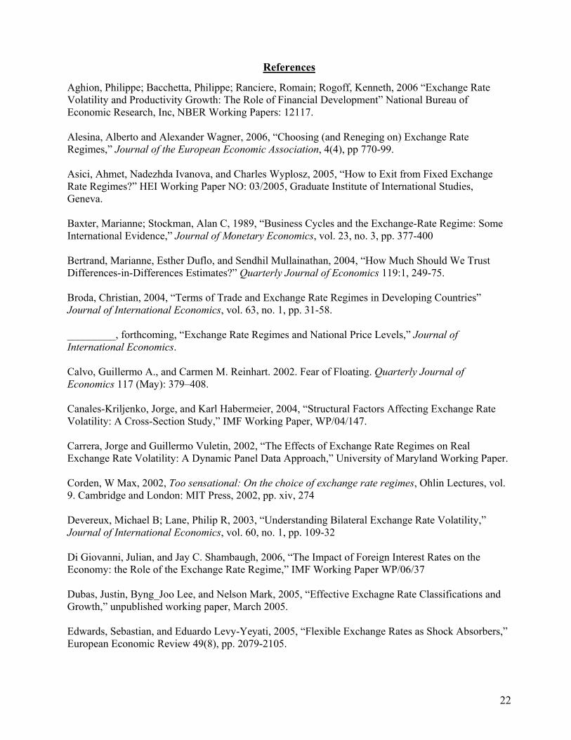
22

References

Aghion, Philippe; Bacchetta, Philippe; Ranciere, Romain; Rogoff, Kenneth, 2006 “Exchange Rate Volatility and Productivity Growth: The Role of Financial Development” National Bureau of Economic Research, Inc, NBER Working Papers: 12117. Alesina, Alberto and Alexander Wagner, 2006, “Choosing (and Reneging on) Exchange Rate Regimes,” Journal of the European Economic Association, 4(4), pp 770-99. Asici, Ahmet, Nadezhda Ivanova, and Charles Wyplosz, 2005, “How to Exit from Fixed Exchange Rate Regimes?” HEI Working Paper NO: 03/2005, Graduate Institute of International Studies, Geneva. Baxter, Marianne; Stockman, Alan C, 1989, “Business Cycles and the Exchange-Rate Regime: Some International Evidence,” Journal of Monetary Economics, vol. 23, no. 3, pp. 377-400 Bertrand, Marianne, Esther Duflo, and Sendhil Mullainathan, 2004, “How Much Should We Trust Differences-in-Differences Estimates?” Quarterly Journal of Economics 119:1, 249-75. Broda, Christian, 2004, “Terms of Trade and Exchange Rate Regimes in Developing Countries” Journal of International Economics, vol. 63, no. 1, pp. 31-58. _________, forthcoming, “Exchange Rate Regimes and National Price Levels,” Journal of International Economics. Calvo, Guillermo A., and Carmen M. Reinhart. 2002. Fear of Floating. Quarterly Journal of Economics 117 (May): 379–408. Canales-Kriljenko, Jorge, and Karl Habermeier, 2004, “Structural Factors Affecting Exchange Rate Volatility: A Cross-Section Study,” IMF Working Paper, WP/04/147. Carrera, Jorge and Guillermo Vuletin, 2002, “The Effects of Exchange Rate Regimes on Real Exchange Rate Volatility: A Dynamic Panel Data Approach,” University of Maryland Working Paper. Corden, W Max, 2002, Too sensational: On the choice of exchange rate regimes, Ohlin Lectures, vol. 9. Cambridge and London: MIT Press, 2002, pp. xiv, 274 Devereux, Michael B; Lane, Philip R, 2003, “Understanding Bilateral Exchange Rate Volatility,” Journal of International Economics, vol. 60, no. 1, pp. 109-32 Di Giovanni, Julian, and Jay C. Shambaugh, 2006, “The Impact of Foreign Interest Rates on the Economy: the Role of the Exchange Rate Regime,” IMF Working Paper WP/06/37 Dubas, Justin, Byng_Joo Lee, and Nelson Mark, 2005, “Effective Exchagne Rate Classifications and Growth,” unpublished working paper, March 2005. Edwards, Sebastian, and Eduardo Levy-Yeyati, 2005, “Flexible Exchange Rates as Shock Absorbers,” European Economic Review 49(8), pp. 2079-2105.

23

Eichengreen, Barry, and Raul Razo-Garcia, 2006, “The Evolution of Exchange Rate Regimes,” Economics Policy, 395-442. Flood, Robert, and Andrew Rose, “Fixing Exchange Rates: A virtual Quest for Fundamentals,” Journal of Monetary Economics, XXXVI (1995), 3-37 Frankel, Jeff, 2003, “Experiences and Lessons of Exchange Rate Regimes in Emerging Economies,” NBER Working Paper No. 10032, October 2003. Friedman, Milton, 1953, “The Case for Flexible Exchange Rates,” in Essays on Positive Economics, (University of Chicago Press, Chicago). Genberg, Hans and Alexander Swoboda, 2005, “Exchange Rate Regimes: Does What Countries Say Matter ?” IMF Staff Papers, Vol 52 (0) 129-41. Ghosh, Anne-Marie Gulde, and Holger Wolf, 2002, Exchange Rate Regimes: Choices and Consequences, MIT Press. Ghosh, Atish, Anne-Marie Gulde, Jonathan Ostry, and Holger Wolf, 1997, “Does the Nominal Exchange Rate Regime Matter?” NBER Working Paper No. 5874. Husain, Aasim M; Mody, Ashoka; Rogoff, Kenneth S, 2005, “Exchange Rate Regime Durability and Performance in Developing versus Advanced Economies” Journal of Monetary Economics, vol. 52, no. 1, pp. 35-64 Kiefer, Nicolas, 1988, “Economic Duration Data and Hazard Functions,” Journal of Economic Literature, vol. 26, no. 2, June, pp. 646 – 679. Klein, Michael W; Shambaugh, Jay C, 2006, “Fixed Exchange Rates and Trade,” Journal of International Economics 70, 359-83. Klein, Michael, and Nancy Marion, “Explaining the Duration of Exchange Rate Pegs,” Journal of Development Economics, LIV (1997), 387-404. Levy-Yeyati, Eduardo; Sturzenegger, Federico, 2003, “To Float or to Fix: Evidence on the Impact of Exchange Rate Regimes on Growth” American Economic Review, vol. 93, no. 4, September 2003, pp. 1173-93 Masson, Paul, 2001, “Exchange Rate Regime Transitions,” Journal of Development Economics 64, pp. 571-86. Masson, Paul, and F.J. Ruge-Muricia, 2005, “Explaining the transition between exchange rate regimes,” Scandinavian Journal of Economics, 107, pp 261-78. Mussa, Michael, 1986, “Nominal Exchange Rate Regimes and the Behavior of Real Exchange Rates: Evidence and Implications” -Carnegie-Rochester Conference Series on Public Policy Obstfeld, Maurice, and Kenneth Rogoff. 1995. The Mirage of Fixed Exchange Rates. Journal of Economic Perspectives 9 (Fall): 73–96.

24

Obstfeld, Maurice; Shambaugh, Jay C; Taylor, Alan M, 2005, “The Trilemma in History: Tradeoffs among Exchange Rates, Monetary Policies, and Capital Mobility,” Review of Economics and Statistics, vol. 87, no. 3, pp. 423-38 Reinhart, Carmen M., and Kenneth S. Rogoff. 2004. The Modern History of Exchange Rate Arrangements: A Reinterpretation. Quarterly Journal of Economics 119 (February): 1-48. Rose, Andrew, 2000. One Money, One Market: The Effect of Common Currencies on Trade. Economic Policy: A European Forum 30, pp. 7-33. Rose, Andrew, 2006, “A Stable International Monetary System Emerges: Inflation Targeting is Bretton Woods, Reversed,” unpublished working paper, October 2006. Shambaugh, Jay C. 2004. The Effects of Fixed Exchange Rates on Monetary Policy. Quarterly Journal of Economics 119 (February): 301-52.

25

Table 1: Basic Statistics on Peg Spells and Float Spells

No. of Annual Obs.

No. of C’ntry

% peg obs.

No. of peg spells

Peg Spell / C. Av’g

Peg Median

Peg Mean

Peg s.d.

No. of float spells

Float Spells / Country Av’g.

Float Median

Float Mean

Float s.d.

Full Sample

3924 125 47.53 398 3.18 2 4.67 6.42 395 3.16 2 5.21 6.69

Industrial Countries

671 21 39.34 56 2.67 2 4.63 6.81 61 2.90 3 6.67 8.88

Developing Countries

3253 104 49.22 342 3.29 2 4.68 6.37 334 3.21 2 4.95 6.18

Sample includes countries for which population > 400,000, USA not in sample, Industrial countries are those with IFS code < 200 but not Turkey nor South Africa, Developing Countries are those with IFS code > 200 and Turkey and South Africa, Currency Unions not included in sample.

Table 2: Peg Spell and Float Spell Survival Statistics (Unconditional), by Spell Peg Spells Float Spells All Countries Industrial Developing All Countries Industrial Developing At least 2 years 55.89% 56.36% 55.81% 64.38% 72.88% 62.75% At least 3 years 40.27% 32.73% 41.61% 48.49% 54.23% 47.39% At least 4 years 34.52% 32.73% 34.84% 38.36% 42.37% 37.58% At least 5 years 30.14% 32.73% 29.68% 33.97% 37.29% 33.33% > 5 years 27.67% 32.73% 26.78% 30.41% 32.20% 30.07% No. of spells 365 55 310 365 59 306 Sample includes countries for which population > 400,000, USA not in sample, Industrial countries are those with IFS code < 200 but not Turkey nor South Africa, Developing Countries are those with IFS code > 200 and Turkey and South Africa, Currency Unions not included in sample.

Table 3: Length of Longest Peg and Float Episode (by country) Length Pegs Length Floats

0 7 6% 0 3 2% 1 8 6% 1 22 18% 2 19 15% 2 5 4% 3 6 5% 3 7 6% 4 7 6% 4 0 0%

5+ 78 62% 5+ 88 70% This table shows the distribution of the longest peg and float episodes by country. There are 125 countries included. For example, 7 countries never peg, 6 have a longest peg of 3 years, and 78 have one of 5 years or more; 3 never float and 88 float for 5 or more consecutive years at some point in the sample.

26

Table 4: Probability of Switching Spell State Next Year, and of Remaining in Same Spell 1, 3, or 5 years in Future, Annual Data

All Countries

Industrial Developing All Countries Industrial Developing

Float(t)|Peg(t-1) 18.43% 17.13% 18.65% Peg(t)|Float(t-1) 16.76% 13.28% 17.63% Peg(t)|Peg(t-1) 81.57% 82.87% 81.35% Float(t)|Float(t-1) 83.24% 86.72% 82.38% Peg(t)|Peg(t-3) 65.75% 71.11% 64.92% Float(t)|Float(t-3) 65.08% 70.23% 63.76% Peg(t)|Peg(t-5) 55.29% 61.69% 54.34% Float(t)|Float(t-5) 54.07% 60.82% 52.28% Years in Peg Spell or in Float Spells. Sample includes countries for which population > 400,000, USA not in sample, Industrial countries are those with IFS code < 200 but not Turkey nor South Africa, Developing Countries are those with IFS code > 200 and Turkey and South Africa, Currency Unions not included in sample. Sample up through 2003 for next year conditional probabilities, up through 2001 for 3 years hence conditional probabilities, and 1999 for 5 years hence conditional probabilities. Countries must remain in same state continuously; that is, Peg(t)|Peg(t-3) suggests staying pegged in (t-3), (t-2), t(-1) and (t). Countries that flip in and out of a state are considered to have broken the state.

Table 5: Conditional Survival Rates by Spell Probability (in percent) of Surviving to year t, given still pegged at year t-1 (initial year of peg or float is Year 1)

Peg Spells Float Spells All Countries Industrial Developing All Countries Industrial Developing Year 2 55.90% 56.14% 55.86% 65.81% 73.77% 64.39% Year 3 70.70% 58.06% 72.83% 75.00% 72.73% 75.48% Year 4 86.09% 100.00% 84.21% 79.89% 78.13% 80.26% Year 5 87.69% 100.00% 85.71% 88.97% 88.00% 89.17% Year 6 91.82% 100.00% 90.22% 89.52% 86.36% 90.20% Years from Beginning of Peg Spell or Beginning of Float Spell. Sample includes countries for which population > 400,000, USA not in sample, Industrial countries are those with IFS code < 200 but not Turkey nor South Africa, Developing Countries are those with IFS code > 200 and Turkey and South Africa, Currency Unions not included in sample.

Table 6: Estimates of Weibull Conditional Hazard Functions Peg Spells Float Spells Coefficient Standard Error Coefficient Standard Error

Previous Spell 0.033** 0.011 0.047** 0.014 Industrial Country 0.256 0.190 0.211 0.175 US Base Dummy 0.650** 0.135

λ 0.844** 0.034 0.912* 0.041 Number of Spells 397 332

* significant at 95% level of confidence, ** at the 99% level for null hypothesis of β = 0 for covariates and null hypothesis of λ = 1 for baseline hazard function parameter.

27

Table 7: Volatility Quintiles Bilateral Volatility Multilateral Volatility

Annual Spell Annual Spell Range %peg Range %peg Range %peg Range %peg 1 .000 – .000 100% .000 - .001 99% .000 - .007 61% .002 - .008 76%

2 .000 - .004 87% .001 - .007 92% .007 - .011 59% .008 - .011 73%

3 .004 - .013 44% .007 - .015 58% .011 - .015 53% .011 - .016 56%

4 .013 - .027 1% .017 - .031 3% .015 - .025 34% .016 - .027 37%

5 .027 – 40.0 0% .031 - 15.0 0% .025 – 1.8 11% .027 - .582 13%

This table shows the % of observations (annual and spell) that are pegged when the data is divided into quintiles by volatility.

Table 8 Exchange Rate Volatility in Spells 1 2 3 4 5 6 7

dep variable bilateral volatility

bilateral volatility

bilateral volatility

bilateral volatility no

first year

bilateral volatility post

79

multilateral multilateral

Sample full drop 1% drop 1% drop 1% drop 1% drop 1% drop 1% FE CFE CFE none CFE CFE CFE CFE Peg -0.158

0.051** -0.068

0.008** -0.065

0.007** -0.045

0.006** -0.081

0.010** -0.022

0.003** -0.008

0.001** spell_bilateral volatility

0.209 0.029**

Constant 0.161 0.026**

0.071 0.004**

0.069 0.007**

0.049 0.004**

0.082 0.005**

0.033 0.001**

0.018 0.002**

Observations R-squared

792 0.17

785 0.31

785 0.14

649 0.3

616 0.35

590 0.45

590 0.74

Smpl mean Smpl sd Smpl med

.082

.689

.010

.036

.086

.010

.036

.086

.010

.021

.052

.008

.041

.097

.010

.022

.026

.013

.022

.026

.013 Peg mean Peg sd Peg med

.004

.004

.003

.004

.004

.003

.004

.004

.003

.004

.004

.003

.004

.004

.003

.012

.009

.010

.012

.009

.010 Nonpeg mean Nonpeg sd Nonpeg med

.161

.971

.025

.069

.112

.024

.069

.112

.024

.048

.075

.023

.079

.128

.023

.032

.033

.019

.032

.033

.019 Note: standard errors clustered at the country level, CFE means country fixed effects, drop 1% drops the 1% largest volatility observations to reduce the impact of outliers. * represents statistically significantly different from zero at the 95% confidence level, ** at the 99% level.

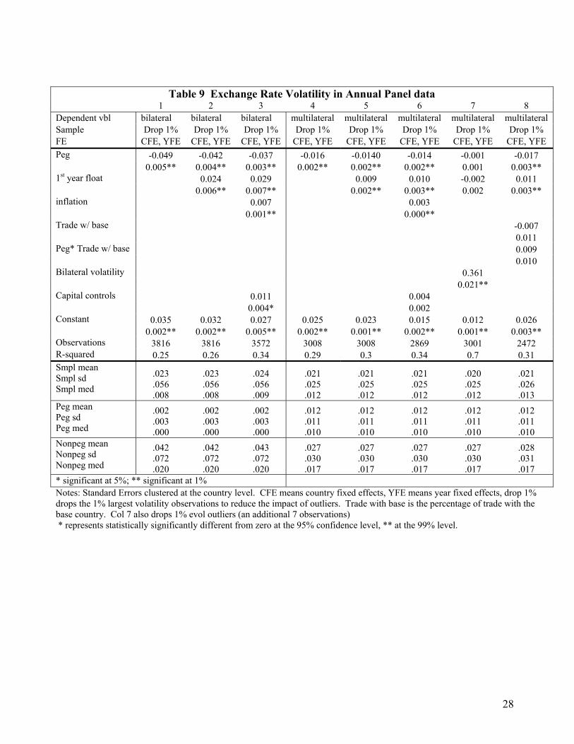
28

Table 9 Exchange Rate Volatility in Annual Panel data 1 2 3 4 5 6 7 8

Dependent vbl bilateral bilateral bilateral multilateral multilateral multilateral multilateral multilateral Sample Drop 1% Drop 1% Drop 1% Drop 1% Drop 1% Drop 1% Drop 1% Drop 1% FE CFE, YFE CFE, YFE CFE, YFE CFE, YFE CFE, YFE CFE, YFE CFE, YFE CFE, YFE Peg -0.049 -0.042 -0.037 -0.016 -0.0140 -0.014 -0.001 -0.017

0.005** 0.004** 0.003** 0.002** 0.002** 0.002** 0.001 0.003** 1st year float 0.024 0.029 0.009 0.010 -0.002 0.011

0.006** 0.007** 0.002** 0.003** 0.002 0.003** inflation 0.007 0.003

0.001** 0.000** Trade w/ base -0.007

0.011 Peg* Trade w/ base 0.009

0.010 Bilateral volatility 0.361

0.021** Capital controls 0.011 0.004

0.004* 0.002 Constant 0.035 0.032 0.027 0.025 0.023 0.015 0.012 0.026

0.002** 0.002** 0.005** 0.002** 0.001** 0.002** 0.001** 0.003** Observations 3816 3816 3572 3008 3008 2869 3001 2472 R-squared 0.25 0.26 0.34 0.29 0.3 0.34 0.7 0.31 Smpl mean Smpl sd Smpl med

.023

.056

.008

.023

.056

.008

.024

.056

.009

.021

.025

.012

.021

.025

.012

.021

.025

.012

.020

.025

.012

.021

.026

.013 Peg mean Peg sd Peg med

.002

.003

.000

.002

.003

.000

.002

.003

.000

.012

.011

.010

.012

.011

.010

.012

.011

.010

.012

.011

.010

.012

.011

.010 Nonpeg mean Nonpeg sd Nonpeg med

.042

.072

.020

.042

.072

.020

.043

.072

.020

.027

.030

.017

.027

.030

.017

.027

.030

.017

.027

.030

.017

.028

.031

.017 * significant at 5%; ** significant at 1% Notes: Standard Errors clustered at the country level. CFE means country fixed effects, YFE means year fixed effects, drop 1% drops the 1% largest volatility observations to reduce the impact of outliers. Trade with base is the percentage of trade with the base country. Col 7 also drops 1% evol outliers (an additional 7 observations) * represents statistically significantly different from zero at the 95% confidence level, ** at the 99% level.

29

Table 10:

Exchange Rate Regime Status in Year Prior to High Volatility outcomes

observations in top 1%

Percent in top 5%

Percent

PANEL A Full sample 3738 37 1.0% 187 5.0% Nonpeg in previous year 1998 21 1.1% 118 5.9% Peg 1740 16 0.9% 69 4.0%

PANEL B Pegged in previous year with peg representing:

1st year of pegging 388 6 1.5% 18 4.6% 2-5 years of pegging 575 5 0.9% 20 3.5% >5 years of pegging 777 5 0.6% 31 4.0%

PANEL C Final year of peg

342

16

4.7%

69

20.2%

1 year peg spell 173 6 3.5% 18 10.4% 2-5 year peg spell 112 5 4.5% 20 17.9% >5 year peg spell 57 5 8.8% 31 54.4% Note: Column 1 shows the total number of observations following a given exchange rate regime status. Column 2 shows how many of those observations are in the top 1% of the volatility distribution.

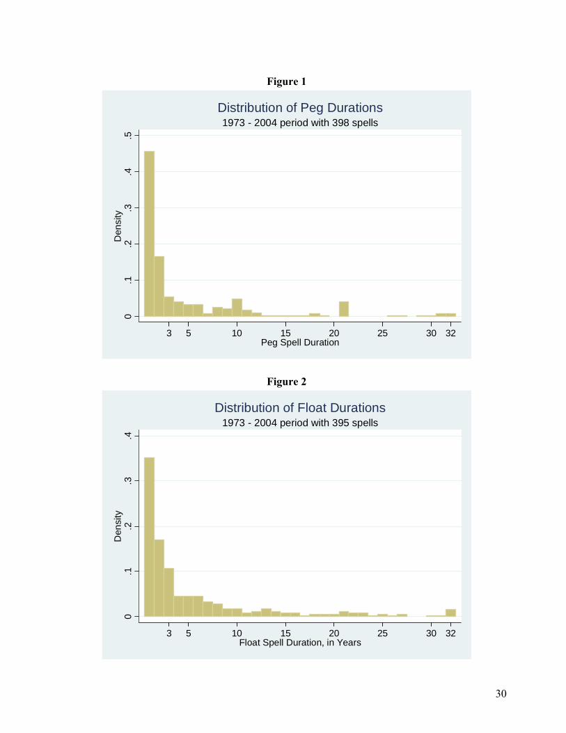
30

Figure 1

0.1

.2.3

.4.5

Den

sity

3 5 10 15 20 25 30 32Peg Spell Duration

1973 - 2004 period with 398 spellsDistribution of Peg Durations

Figure 2

0.1

.2.3

.4D

ensi

ty

3 5 10 15 20 25 30 32Float Spell Duration, in Years

1973 - 2004 period with 395 spellsDistribution of Float Durations

31

Figure 3 Long-lived pegs

Number of pegs that have lasted 5 years over time

05

101520253035404550

1978

1980

1982

1984

1986

1988

1990

1992

1994

1996

1998

2000

2002

2004

Figure shows the number of countries in a peg that has lasted for more than 5 years at that moment. The panel is roughly balanced with between 122 and 125 countries in the sample. Currency unions are eliminated from sample

with the exception of spells that began as pegs and converted to currency unions (some EMU observations).

Figure 4a and b: Volatility over time Bilateral Volatility over time Multilateral Volatility over time

-0.07

-0.06

-0.05

-0.04

-0.03

-0.02

-0.01

0

0.01

0 1 2 3 4 5

-0.07

-0.06

-0.05

-0.04

-0.03

-0.02

-0.01

0

0.01

0 1 2 3 4 5

Note: time zero represents the contemporaneous coefficient of exchange rate volatility on pegging. Time 1 represents the coefficient on a lagged peg and so on. Thus the point at “2” represents the difference in volatility for a country that was pegged two years ago (whether it has remained pegged or not). Country and year fixed effects are included. The dark lines represent 2 times standard error bands around the main point estimates where standard errors are clustered on country. To insure that the comparison is with nonpegged observations, new pegs that are not repegs are excluded (see text). Squares represent the point estimate if the first year of pegging is excluded.

32

Appendix: Comparing Classification Schemes

A1. Different Classifications Schemes:

As mentioned in the text, we employ a classification scheme in this paper in which a peg spell is defined as a situation where, over the course of a calendar year, the month-end bilateral exchange rate with the base country stays within a 2% band. This classification scheme, which we call KS in this appendix, is similar in spirit to that used by Obstfeld and Rogoff (1995), although that paper did not provide an extensive classification of all countries as pegged or not pegged. In this appendix we compare this classification scheme to those used by Shambaugh (2004) (hereafter “JS”), Reinhart Rogoff (2004) (hereafter RR), Levy-Yeyati and Sturzenegger (2003) (hereafter LYS) and the declared or de jure regimes (hereafter “DJ”) (Calvo and Reinhart (2004) focus on de jure regimes).

The KS classification scheme is most similar to the JS classification scheme, which was used to test the policy trilemma. The two principal differences between the KS and JS classification schemes are that the latter excludes one year pegs and also the latter allows a peg spell to continue if there is a one-time discrete devaluation during a year. Thus, comparisons between the KS and JS classification schemes show the effect of these two conditions since, but for the treatment of one year pegs and discrete devaluations, they are quite similar.

The RR classification scheme was developed to study the evolution of policy regimes. It focuses on the conditional probability of the exchange rate staying within a given range over a rolling five year window, and it also uses information about parallel (dual market) exchange rates in determining whether a peg continues from one year to the next. This classification scheme allows devaluations to occur within a peg spell so, consequently, it results in fewer peg spells and peg spells of longer duration than the KS classification scheme. (see also Section II and its footnotes for further discussion).43

LYS differs from the other classification schemes discussed here in its use of information on reserves. Cluster analysis and information on reserves/M2 volatility, exchange rate volatility, and volatility of the change in the exchange rate is used by Levy-Yeyati and Sturzenegger to sort observations into pegs, intermediate regimes, and floats. One result of this use of cluster analysis is that about half of the countries with an unvarying exchange rate, those with no reserve volatility or without reserve data, are coded as “ad hoc” pegs since the cluster analysis initially places these cases in an “inconclusive” category. Another result of the cluster analysis is that the LYS classification scheme results in far more pegs than other classifications, partly because observations with a fair amount of exchange rate volatility may, nonetheless, be classified as pegs if there is also substantial change in reserves/M2. The LYS coding does not, however, include most years with a discrete devaluation from one fixed rate to another as a peg year because the change in the exchange rate relative to the change in reserves volatility is gauged as being too large to be a peg in those cases. Thus, this classification scheme does not include as pegs many of the highest volatility outcomes that RR and JS code as pegs.

The DJ coding is the most straightforward classification scheme, simply representing the regime declared to the IMF and reported in the IMF’s annual yearbook on exchange rate arrangements. 43 We use the Reinhart Rogoff annual data set from Carmen Reinhart’s website extended to 2004 with data from Eichengreen and Razo-Garcia on Barry Eichengreen’s website.

33

A2. Correlations of Pegging and Floating Across Classification Schemes: Table A1 presents the percentage of observations for which binary versions of each classification scheme agree with one another as well as the percentage coded as pegged.44 The statistics in this table show that the classification schemes are broadly similar, but differ in somewhat systematic ways that generate different results on a number of areas of our analysis. See also Shambaugh (2004) or Frankel (2003) for comparisons of different de facto classification schemes.

Table A1: Percentage agreement of various coding methodologies for our sample

Peg jspeg rrpeg Djpeg

% obs coded as pegged

Peg 1 47% Jspeg 93% 1 45% Rrpeg 80% 82% 1 33% Djpeg 81% 86% 81% 1 41% Lyspeg 81% 80% 73% 74% 58%

Note: This table shows the percentage of observations where different codings yield the same result as one another. “peg” is the classification used in the paper. “jspeg” is the JS coding, “rrpeg” is the RR coding, “djpeg” is the de jure coding, and lyspeg is the LYS classification. All codings are collapsed to a binary peg and nonpeg coding. The final column shows the percent of observations coded as pegged by each classification.

A3. Spell Lengths Across Classification Schemes: The spell length and number of spells is the category for which the results differ most across classification schemes. Table A2 presents statistics illustrating this by reproducing Table 1 in the text for the different classification schemes.

Table A2 shows that the RR classification scheme identifies far fewer spells and, accordingly, much longer duration than the others. The RR median peg length is 8 years, and the RR mean peg length is 12 years. Floats are even more durable in the RR classification scheme, with a mean and median of 20 years. This long duration is a consequence of the effort to identify overall policy regimes as opposed to specific peg spells. The RR classification scheme involves a great deal of smoothing due to the use of the conditional probability of staying within a range over a five year period.45 Contrast this with the statistics presented in Table A2 for the JS classification scheme. The JS classification scheme, like RR, allows devaluations and drops single year pegs but it differs from RR in its focus on annual patterns and in that it does not smooth regime switches. The peg spell median in the JS classification scheme is 5 years, the mean is 9 years, the float spell median is 7 years and the mean is 11 years. A specific example also illustrates the difference between the JS and RR classification schemes: RR codes France as not pegged at all from 1973-86 and pegged throughout thereafter while JS (and KS) identify the short-lived pegs in 1979-80 and 1984-5. The DJ coding also

44 For RR, mgcode = 1 is considered a peg (this includes pre-announced pegs, horizontal bands that are narrower or equal to +/-2%, and de facto pegs. For DJ, peg is defined as pegs, limited flexibility, and cooperative agreements (the EMS). 45 As an example of this, consider the results presented in Husain et al. who use the Reinhart Rogoff classification scheme. They report an average peg spell duration of 28 years. There are a number of reasons beyond coding for such a large average. They have a much longer sample and as such, very long regimes will affect the average (medians are not reported). In addition, they include very small countries (eliminated in Obstfeld and Rogoff) which have much longer spells and include some long run currency unions (such as Panama).

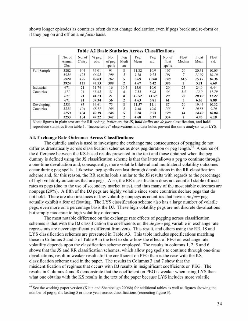
34

shows longer episodes as countries often do not change declaration even if pegs break and re-form or if they peg on and off on a de facto basis.

Table A2 Basic Statistics Across Classifications No. of

Annual Obs.

No. of C’ntry

% peg obs.

No. of peg spells

Peg Medi

an

Peg Mean

Peg s.d.

No. of float spells

Float Median

Float Mean

Float s.d.

Full Sample 3202 3924 3924 3924

104 125 125 125

34.01 46.02 42.03 47.53

91 199 167 398

8 5 5 2

11.82 9.16 9.69 4.67

10.9 9.75

10.00 6.42

107 191 148 395

20 7

14.5 2

20.31 11.09 15.17 5.21

10.05 10.10 10.36 6.69

Industrial Countries

671 671 671 671

21 21 21 21

31.74 35.62 41.23 39.34

16 31 21 56

10.5 6 8 2

13.0 7.55 12.52 4.63

10.0 8.08

11.57 6.81

20 36 20 61

25 5.5 23 3

24.0 12.0

20.10 6.67

6.44 11.79 11.27 8.88

Developing Countries

2531 3253 3253 3253

83 104 104 104

34.61 48.17 42.19 49.22

75 168 146 342

8 5 5 2

11.57 9.46 9.28 4.68

11.1 10.0 9.73 6.37

87 155 128 334

20 8

14 2

19.46 10.88 14.40 4.95

10.32 9.70 10.04 6.18

Note: figures in plain text are for RR coding, italics are for JS, bold italics are de jure classification, and bold reproduce statistics from table 1. “Inconclusive” observations and data holes prevent the same analysis with LYS.

A4. Exchange Rate Outcomes Across Classifications: The quintile analysis used to investigate the exchange rate consequences of pegging do not differ as dramatically across classification schemes as does peg duration or peg length.46 A source of the difference between the KS-based results presented in the text and those obtained when the peg dummy is defined using the JS classification scheme is that the latter allows a peg to continue through a one-time devaluation and, consequently, more volatile bilateral and multilateral volatility outcomes occur during peg spells. Likewise, peg spells can last through devaluations in the RR classification scheme and, for this reason, the RR results look similar to the JS results with regards to the percentage of high volatility outcomes that are pegs. Also, the RR classification does not count all stable official rates as pegs (due to the use of secondary market rates), and thus many of the most stable outcomes are nonpegs (29%). A fifth of the DJ pegs are highly volatile since some countries declare pegs that do not hold. There are also instances of low volatility nonpegs as countries that have a de jure peg actually exhibit a fear of floating. The LYS classification scheme also has a large number of volatile pegs, even more on a percentage basis the DJ. These high volatility pegs are not discrete devaluations but simply moderate to high volatility outcomes.

The most notable difference on the exchange rate effects of pegging across classification schemes is that with the DJ classification the coefficients on the de jure peg variable in exchange rate regressions are never significantly different from zero. This result, and others using the RR, JS and LYS classification schemes are presented in Table A3. This table includes specifications matching those in Columns 2 and 5 of Table 9 in the text to show how the effect of PEG on exchange rate volatility depends upon the classification scheme employed. The results in columns 1, 2, 5 and 6 shows that the JS and RR classification schemes, which allow peg spells to continue through one-time devaluations, result in weaker results for the coefficient on PEG than is the case with the KS classification scheme used in the paper. The results in Columns 3 and 7 show that the misidentification of regimes that occurs with DJ results in insignificant coefficients on PEG. The results in Columns 4 and 8 demonstrate that the coefficient on PEG is weaker when using LYS than what one obtains with the KS results in the text of the paper because LYS includes more volatile 46 See the working paper version (Klein and Shambaugh 2006b) for additional tables as well as figures showing the number of peg spells lasting 5 or more years across classifications (recreating figure 3).

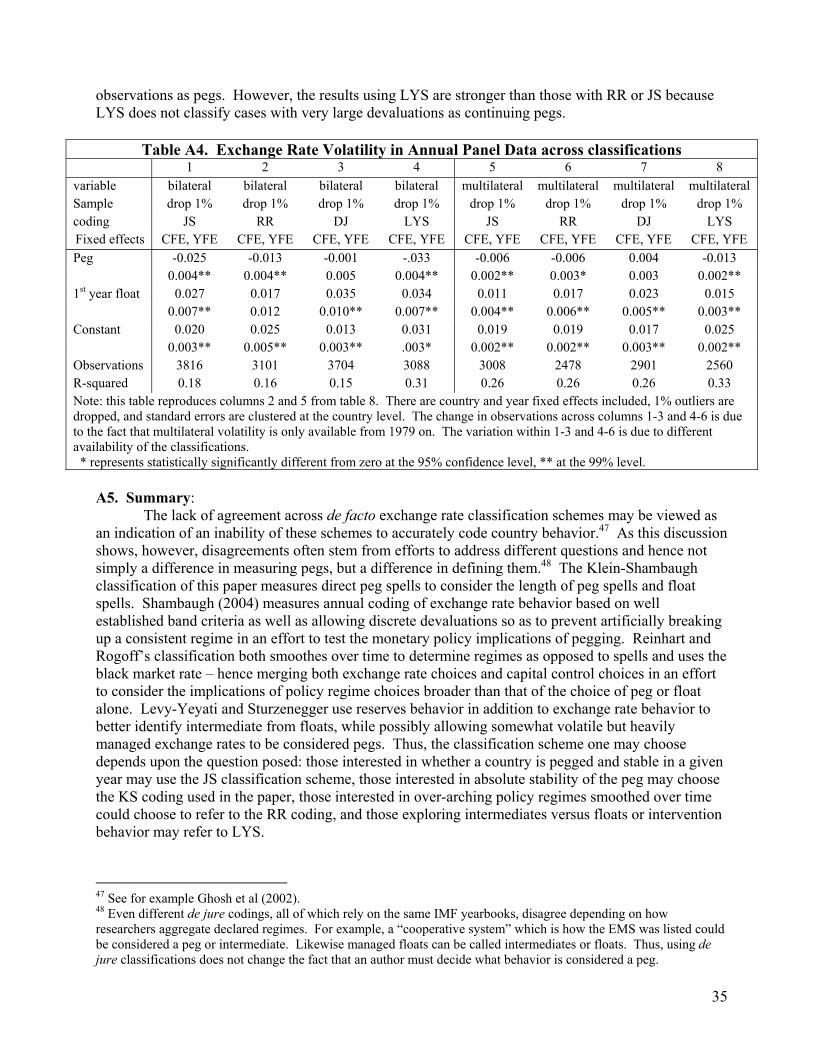
35

observations as pegs. However, the results using LYS are stronger than those with RR or JS because LYS does not classify cases with very large devaluations as continuing pegs.

Table A4. Exchange Rate Volatility in Annual Panel Data across classifications 1 2 3 4 5 6 7 8

variable bilateral bilateral bilateral bilateral multilateral multilateral multilateral multilateral Sample drop 1% drop 1% drop 1% drop 1% drop 1% drop 1% drop 1% drop 1% coding JS RR DJ LYS JS RR DJ LYS Fixed effects CFE, YFE CFE, YFE CFE, YFE CFE, YFE CFE, YFE CFE, YFE CFE, YFE CFE, YFE Peg -0.025 -0.013 -0.001 -.033 -0.006 -0.006 0.004 -0.013

0.004** 0.004** 0.005 0.004** 0.002** 0.003* 0.003 0.002** 1st year float 0.027 0.017 0.035 0.034 0.011 0.017 0.023 0.015

0.007** 0.012 0.010** 0.007** 0.004** 0.006** 0.005** 0.003** Constant 0.020 0.025 0.013 0.031 0.019 0.019 0.017 0.025

0.003** 0.005** 0.003** .003* 0.002** 0.002** 0.003** 0.002** Observations 3816 3101 3704 3088 3008 2478 2901 2560 R-squared 0.18 0.16 0.15 0.31 0.26 0.26 0.26 0.33 Note: this table reproduces columns 2 and 5 from table 8. There are country and year fixed effects included, 1% outliers are dropped, and standard errors are clustered at the country level. The change in observations across columns 1-3 and 4-6 is due to the fact that multilateral volatility is only available from 1979 on. The variation within 1-3 and 4-6 is due to different availability of the classifications. * represents statistically significantly different from zero at the 95% confidence level, ** at the 99% level.

A5. Summary:

The lack of agreement across de facto exchange rate classification schemes may be viewed as an indication of an inability of these schemes to accurately code country behavior.47 As this discussion shows, however, disagreements often stem from efforts to address different questions and hence not simply a difference in measuring pegs, but a difference in defining them.48 The Klein-Shambaugh classification of this paper measures direct peg spells to consider the length of peg spells and float spells. Shambaugh (2004) measures annual coding of exchange rate behavior based on well established band criteria as well as allowing discrete devaluations so as to prevent artificially breaking up a consistent regime in an effort to test the monetary policy implications of pegging. Reinhart and Rogoff’s classification both smoothes over time to determine regimes as opposed to spells and uses the black market rate – hence merging both exchange rate choices and capital control choices in an effort to consider the implications of policy regime choices broader than that of the choice of peg or float alone. Levy-Yeyati and Sturzenegger use reserves behavior in addition to exchange rate behavior to better identify intermediate from floats, while possibly allowing somewhat volatile but heavily managed exchange rates to be considered pegs. Thus, the classification scheme one may choose depends upon the question posed: those interested in whether a country is pegged and stable in a given year may use the JS classification scheme, those interested in absolute stability of the peg may choose the KS coding used in the paper, those interested in over-arching policy regimes smoothed over time could choose to refer to the RR coding, and those exploring intermediates versus floats or intervention behavior may refer to LYS.

47 See for example Ghosh et al (2002). 48 Even different de jure codings, all of which rely on the same IMF yearbooks, disagree depending on how researchers aggregate declared regimes. For example, a “cooperative system” which is how the EMS was listed could be considered a peg or intermediate. Likewise managed floats can be called intermediates or floats. Thus, using de jure classifications does not change the fact that an author must decide what behavior is considered a peg.